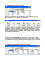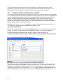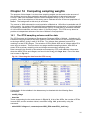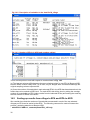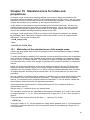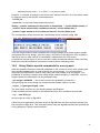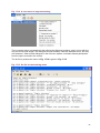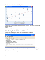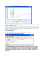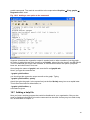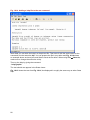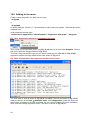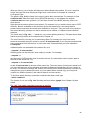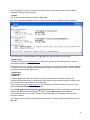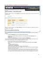
1
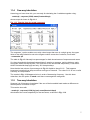
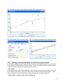
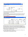
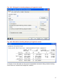
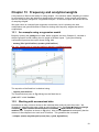
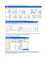
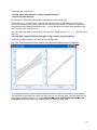
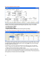
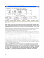
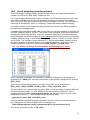
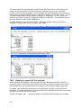
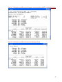
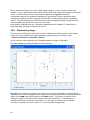
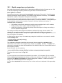
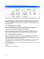
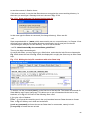
Fig 16.4 Plot of model residuals versus fitted values
For the residual term to have constant variance the plot of residuals against fitted/predicted
values should show no obvious departures from a random scatter. Fig. 16.4 shows no
recognisable pattern, so the assumptions behind our model appear tenable and interpretation of
its results is safe. We can now proceed to present estimates and their standard errors.
16.6
Reporting the results
The next step is to obtain the estimates of the 4 parameters of the regression lines, i.e. 3
separate intercepts and one common slope use:
. anova yield fertiliser varietyn, category(varietyn) regress noconstant
The resulting output appears in Fig. 16.5: Ignore the ANOVA table with a single row for the
combined model and focus on the table of parameter estimates with their 95% confidence
intervals.
Note the use of the regress and noconstant options: while the former prints the table of
parameter estimates of the linear model, the latter gives these parameters as absolute values
instead of differences from a reference level, as is done by default in most statistics software.
Absolute values are useful here in order to present 3 predictive equations, one for each variety.
From Fig 16.5, the equations for predicting yield of each variety are:
yield of NEW variety = 47.75 + 5.26x
yield of OLD variety = 35.69 + 5.26x
yield of TRAD variety = 25.96 + 5.26x
where x is a set amount of fertiliser in the observed range of 0 to 3 units.
The intercept is the estimated yield of each variety at x=0, i.e. when no fertiliser is applied. The
increase in yield for each 1 extra unit of fertiliser applied is estimated at 5.26 yield units. Finally,
we are 95% confident that the range 3.3 to 7.2 yield units contains the true value of the rate of
increase, which is common to all 3 varieties.
53