Download Icon

Faculty of Science and Technology
MASTER’S THESIS
Study program/ Specialization:
Spring semester, 2014
Master of Science in Computer Science
Open / Restricted access
Writer: Nigussie Girma Tulu
…………………………………………
(Writer’s signature)
Faculty supervisor:
Reggie Davidrajuh
Thesis title:
Monitor for displaying the status of Real-Time simulation.
Credits (ECTS): 30 ECTS
Key words:
Pages: 166
Discrete Event Dynamic Systems (DEDS)
Real-Time (R-T)
Petri net (P-N)
GpenSIM
MATLAB GUIDE
NXT device
+ enclosure: CD
Stavanger, 26 June, 2014
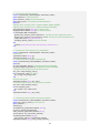
Summary
This paper presents a design and implementation of a monitor to display the status of realtime simulation and modelling for discrete event dynamic systems, DEDS. The modelling
and simulation of DEDS in this thesis are implemented using two kinds tools called Petri net
and GpenSIM. Petri Nets are tools that are widely used now a day to model and simulate
discrete events of concurrent and dynamic systems. [1] Petri net has a graphical formalism
that is getting popularity in recent years as a tool for representing complex mathematical
and analytical interactions (like synchronization, concurrency, atomicity, sequential and
conflict control) among physical components or activities in DEDS. [1] Besides a Petri net
can be primarily used for analyzing and modeling the dynamic and concurrent behavior of
distributed systems where there is a discrete event flow. GPenSim, where this thesis will
rely on, is a general purpose Petri net simulation tool used to model and simulate systems
of discrete events that are designed using a Petri Net tool. In this thesis, a human computer
interaction (HCI) tool for GpenSIM is also introduced. This is because of the fact that
GPenSIM doesn’t provide a method to display the simulation process on a graphical display
unit. The newly implemented HCI tool is used for displaying the status of the running
GpenSIM file on a monitor screen; it has also an enhanced tool that helps the user to easily
control the Real-Time simulation process. To illustrate the application of Real-Time
simulation and modelling using Petri net and to test the newly developed HCI tool for
GpenSIM, it has also been implemented different kind of real life models in some
application areas like industry, traffic light signal and door alarm. In this thesis, NXT
intelligent brick with sensors have been used to show how GpenSIM works for modelling
the real life system run on Real-Time and also to illustrate the modelling power of a Petri
net by testing the newly implemented display tool. The NXT Intelligent brick is a simple
robotic device that is built for educational purpose. [2] The device is used to get a RealTime data from different sensor nodes on Real-Time.
i
Acknowledgment
First of all I would like to thank God for making me stronger and giving me the power to
pursue my thesis work. Next I would like to thank my Supervisor prof. Reggie Davidrajuh for
his endless support starting from day one up to my final submission. He was always
encouraging me to create new ideas. I would like also to thank Ståle Freie for borrowing me
all the necessary lab equipment and also for letting me to use the lab at any time I want. At
Last but not least I would like to thank my lovely fiancé, Arsema Takele, and my lovely
daughter, Atnasia Nigussie, for understanding and giving me more energy throughout my
study, I couldn’t be at this stage if it wasn’t for them. I would like also to thank my whole
family specially my sister, Alemtsehay Girma, for encouraging me to work harder. I would
like also to thank all of my friends and my classmates for having wonderful times together.
ii
Contents
Summary .............................................................................................................................................. i
Acknowledgment ................................................................................................................................ ii
Contents............................................................................................................................................. iii
Notations ........................................................................................................................................... vi
Chapter 1 ............................................................................................................................................ 1
1.
Introduction ............................................................................................................................ 1
1.1
Motivation .............................................................................................................................. 1
1.2
Goal of the thesis .................................................................................................................... 2
1.3
Adaptations............................................................................................................................. 6
1.4
Chapters review ...................................................................................................................... 6
Chapter 2 ............................................................................................................................................ 8
2.
Background ............................................................................................................................. 8
2.1
Systems, modelling and simulation ........................................................................................ 8
2.2
Discrete events dynamic systems (DEDS) ............................................................................. 10
2.3
Continuous event time simulation ....................................................................................... 12
2.4
Petri Net ................................................................................................................................ 12
2.4.1 Places .................................................................................................................................... 13
2.4.2 Transition .............................................................................................................................. 14
2.4.3 Arcs ....................................................................................................................................... 14
2.4.4 Arc Weight ............................................................................................................................ 15
2.4.5 Tokens ................................................................................................................................... 15
2.4.6 Mathematical representation of a Petri Net ........................................................................ 15
2.4.7 Firing Sequence and firing time ............................................................................................ 16
2.5
Extended Petri net ................................................................................................................ 16
2.5.1 Timed Petri Nets ................................................................................................................... 17
2.5.2 Stochastic Timed Petri Nets .................................................................................................. 17
2.5.3 Color Petri net (CPN) ............................................................................................................. 17
2.6
GPenSIM ............................................................................................................................... 17
2.6.1 The Structure of GPenSIM .................................................................................................... 18
2.6.2 The main simulation file (MSF file) ....................................................................................... 19
2.6.3 The Petri net definition file (PDF file) ................................................................................... 19
iii
2.6.4 The transitional definition file .............................................................................................. 19
Chapter 3 .......................................................................................................................................... 23
3.
Overview of Real-time simulation and some application ..................................................... 23
3.1
Real-Time simulation and modelling .................................................................................... 23
3.2
Real-Time Simulation using GPenSIM ................................................................................... 24
3.2.1 Real-Time simulation in Industrial application ..................................................................... 26
3.2.2 Real-Time simulation in room security ................................................................................. 27
3.3
Real-Time simulation and modelling using NXT machine .................................................... 31
3.3.1 NXT Mindstrom device. ........................................................................................................ 31
3.3.2 Door alarm system using NXT ............................................................................................... 32
3.3.3 Traffic light system modeled using NXT intelligent Brick ..................................................... 37
Chapter 4 .......................................................................................................................................... 43
4.
Designing R-T monitor for GPenSIM ..................................................................................... 43
4.1
Human Computer Interactions, HCI...................................................................................... 43
4.2
Design R-T display system ..................................................................................................... 44
4.3
User interfaces design .......................................................................................................... 45
4.3.1 Graphical user interface (gui) basics. .................................................................................... 46
4.3.2 MATLAB GUIDE ..................................................................................................................... 46
4.4
R-T monitor user interfaces .................................................................................................. 51
4.4.1 Design of an interface to select a Real-Time places and transitions .................................... 51
4.4.2 Design of a graphical display system for Real-Time Monitor (GUI main) ............................. 53
Chapter 5 .......................................................................................................................................... 62
5.
Implementation .................................................................................................................... 62
5.1
Implementation of R-T monitor. ........................................................................................... 63
5.1.1 Implementation of a user interface to select places and transitions. .................................. 65
5.1.2 Implementation of graphical Display for Real-Time Monitor ............................................... 69
5.1.3 Other implementations of R-T monitor ................................................................................ 76
5.2
Implementation of gpensim code for the real-time models ................................................ 88
5.2.1 Implementation of R-T simulation in Industrial application ................................................. 88
5.2.2 Implementation of R-T simulation in door security using gpensim...................................... 89
5.2.3 Implementation of R-T door alarm system using NXT .......................................................... 90
5.2.4 Implementation of R-T City Traffic light system using NXT [39] ........................................... 93
Chapter 6 .......................................................................................................................................... 96
6.
Experimentation and Analysis .............................................................................................. 96
iv
6.1
Experimentation for R-T simulation in section 5.2 ............................................................... 96
6.1.1 Test results for R-T simulation in Industrial application. ...................................................... 96
6.1.2 Test results For NXT door alarm model ................................................................................ 99
6.1.3 Test results for traffic light system ..................................................................................... 104
Chapter 7 ........................................................................................................................................ 111
7.
Discussion and conclusion .................................................................................................. 111
7.1
Discussion ........................................................................................................................... 111
7.2
Further Improvement ......................................................................................................... 112
7.3
Conclusion........................................................................................................................... 113
References ...................................................................................................................................... 114
Appendix A ...................................................................................................................................... 117
Appendix B ...................................................................................................................................... 121
Appendix C ...................................................................................................................................... 122
v
Notations
P-N
Petri net
PN
Structure data type in GPenSIM.
R-T
Real-Time
DEDS
Discrete event Dynamic Systems
GPenSIM
General Purpose Petri net simulator
gpensim
GPenSIM system file
MSF
Main simulation file
PDF
Petri net Definition file
TDF
transitional definition file
HCI
Human computer interaction
NXT
LEGO Mindstrom microcontroller device
MATLAB GUIDE
A MATLAB graphical user interface layout designer tool
GCBO
a MATLAB variable automatically created each time a callback is
executed, and returns the handle of the object.
gcf
A MATLAB command creates an empty figure.
GUI.m
Background MATLAB script file for R-T monitor display.
GUI.fig
MATLAB designer layout file for R-T monitor display
Real_PTtime_select.m
Background MATLAB script file to select places and transitions.
Real_PTtime_select.fig
MATLAB designer layout file for Real_PTtime_select.m
FCS
firing condition satisfied
,, 
Measuring parameters
 , , 
Symbols that denote Events
 , t, 
Symbols that denote time frame
gui_singleton
GUIDE command to control the number of opened gui windows
Callback
The background event handling function in MATLAB GUIDE
GUI
The Main display in the new implemented R-T monitor
gui
graphical user interface
vi
vii
Chapter 1
1. Introduction
The field of Simulation and modelling is one of the rapidly developing area in computer
science. [3] Different scientific areas introduce the need for modelling and simulation
according to their basic necessities. It is well known that computers have changed the way
we used to live not only by assisting on the day to day activities but also by letting to model
the actual system and enable us to predict about the future work. The technique of
modelling real life activities is called simulation and modelling. It is obvious that most part
of our day to day activities, starting from counting time notion, are more or less related to
mathematics. Since mathematical formulations have powerful tools to represent the actual
system and our day to day activities that are associated with Real-Time, systems can be
modeled using mathematical tools based on a Real-Time. The terms "modeling" and
"simulation" are often used interchangeably. Thus this thesis discusses about the basic
method of modellings and simulation using the appropriate tools in Real-Time. The
implementations were carried out on a MATLAB studio using a MATLAB language. It has
also been used an NXT Mindstrom microcontroller with different types of sensors to get a
Real-Time data input from some sensor nodes. The simulations were designed and
implemented using a GPenSIM and Petri net tools. The current version of GPenSIM runs in
two modes, these are using either:
1) Simulated clock
2) Real-time clock
When the real-time clock is used, the simulation is actually performing real-time control
activity, like reading sensor (input) data, making control policy, and then feeding the
actuators (outputs) with control (output) data. The idea was adapted from the work of prof.
Davidrajuh ‘GPenSIM in Real-Time’.
1.1
Motivation
The task of designing, evaluating, developing a discrete event dynamics systems, DEDS, in a
Real-Time systems requires a deep knowledge of modelling and decision making rules for
an intelligent system. One might get it very difficult to design a DEDS unless a proper tool is
used. But using the available tools like Petri net and the simulation software gpensim, it can
be simplified; even can one develop a system that is more dynamic and intelligent. The
1
Petri net model for Fuzzy, Adaptive and Expert System Controller, integrated into the
GPenSIM Simulation Tool Kit, has greatly facilitated this task.
Usually, the proving of validity of models is an interesting task, because even if an excellent
simulator is running on an excellent hardware, the simulation results of inaccurate model
will never be valid. Especially for real-time simulation, the data of R-T simulation are large
and needs a proper management to achieve validity. For a DEDS, one of the ways that we
can improve the performance of a simulation and modelling is that if it is possible to watch
the movement of every tokens and the status of each event during a simulation process.
Even it would be very easy to control the process by putting the unwanted redundant
information into the background and making only the valuable units visible for the user.
1.2
Goal of the thesis
The main objective of the thesis was roughly discussed in the summery section above. The
current version of GPenSIM doesn’t have a method to display the Real-Time simulation
process of DEDS on a visual interaction unit, HCI tool. I.e. it doesn’t have a mechanism to
graphically display the status of every transition and their associated input/output places,
and the number of tokens in every place during every simulation cycle. Besides; GPenSIM
lacks a method to control the speed and process of the simulation. The current version of
GPenSIM stores the simulation results in some form of ASCII dump file, log file and the
result is displayed using a MATLAB command window. Similarly the status of the simulation
is displayed using the normal MATLAB ‘disp’ function. This is quite infeasible when we think
of Real-Time systems where the actual progress of the simulation is running on a Real-Time.
If we consider a system with a lot of sensors and actuators which are running on real-time,
It would be better to have a method to capture the ongoing process rather than going back
and evaluating the damped ASCII code files. A good example is simulation in industrial
application where there are different production line and the status of the lines are
represented as Petri net transitions. It would be tedious and impractical if we let the
simulation file to be stored as a dump log file and retrieve it for analysis, thus the best way
would be designing a visual aid tool to interact with the background system and to see the
actual ongoing progress.
The newly implemented tool acquires GPenSIM to have an enhanced tool to work with the
simulation operation of the P-N model, i.e. there is a control button on the interface unit
which would help the user to control the ongoing system with time by watching the
progress on a single display. Generally, since time is a key value in Real-Time simulation, it
2
can be very difficult to overview the results of a simulation that are only presented in a text
log file, especially for larger models, it can be more complicated.
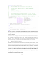
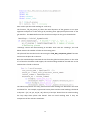
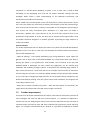
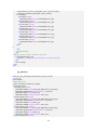
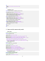
The following figures show the difference between the two results, i.e. the result of the
current GPenSIM simulation and the newly implemented tool.
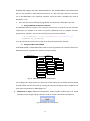
For the example mentioned above, suppose we have three production lines that read input
from a source input and put the result on a buffer.
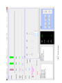
The ASCII dump file is:
======= State Diagram =======
** Time: 08:34:03 **
State:0 (Initial State): (no tokens)
At start ....
At time: 08:34:03, Enabled transitions are: tInPut
At time: 08:34:03, Firing transitions are: tInPut
** Time: 08:34:09 **
State: 1
Fired Transition: tInPut
pInout_Buff +
pInout_Buff +
pInout_Buff +
pInout_Buff +
pInout_Buff +
Current State: pInout_Buff
Virtual tokens: (no tokens)
Right after new state-1 ....
At time: 08:34:10, Enabled transitions are:
tInPut tProduction_line1
tProductionline3
At time: 08:34:10, Firing transitions are: tInPut tProduction_line1
** Time: 08:34:11 **
State: 2
Fired Transition: tProduction_line1
pOutPut1 +
pOutPut1 +
pOutPut1 +
pOutPut1 +
Current State: pOutPut1
Virtual tokens: (no tokens)
Right after new state-2 ....
At time: 08:34:11, Enabled transitions are: tInPut
At time: 08:34:11, Firing transitions are: tInPut
Virtual tokens: (no tokens)
.
.
.
3
tProduction_line2
** Time: 08:34:20 **
State: 12
Fired Transition: tInPut
pInout_Buff +
pInout_Buff + 2pOutPut1 +
pInout_Buff + 2pOutPut1 +
pInout_Buff + 2pOutPut1 +
pInout_Buff + 2pOutPut1 + pOutput_Buffer +
Current State: pInout_Buff + 2pOutPut1 + pOutput_Buffer
Virtual tokens: (no tokens)
Right after new state-12 ....
At time: 08:34:20, Enabled transitions are:
tInPut tProduction_line1
tProductionline3
At time: 08:34:20, Firing transitions are: tInPut tProduction_line1
tProduction_line2
.
.
.
** Time: 08:34:32 **
State: 24
Fired Transition: tProduction_line2
3pOutPut1 +
3pOutPut1 + 2pOutput2 +
3pOutPut1 + 2pOutput2 +
3pOutPut1 + 2pOutput2 + 2pOutput_Buffer +
Current State: 3pOutPut1 + 2pOutput2 + 2pOutput_Buffer
Virtual tokens: (no tokens)
Right after new state-24 ....
At time: 08:34:32, Enabled transitions are: tInPut
At time: 08:34:32, Firing transitions are: tInPut
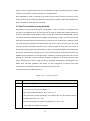
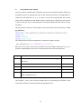
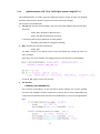
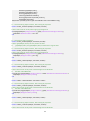
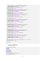
The above text is taken from a large gpensim simulation result as a sample, as it is very
large text and takes a large area to show on this paper. As stated above, GPenSIM stores
this result as a log file and printed on a MATLAB command window.
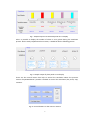
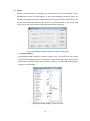
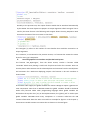
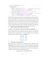
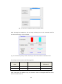
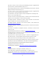
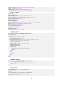
The associated result on a newly implemented R-T monitor would be as follow.
4
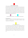
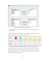
Fig. I. Sample output of Transitional panel on R-T display
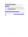
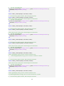
Also it is possible to display the number of token in every places during the simulation
process. On the newly implemented R-T monitor, it would be like the following picture.
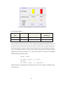
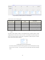
Fig. II. Sample output of place panel on R-T display
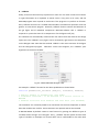
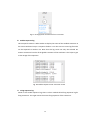
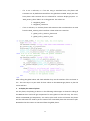
There are also control button that help to control the simulation where the previous
version of GpenSIM doesn’t provide a method to control the simulation, like pause, stop,
continue.
Fig. III. Control buttons on the new R-T monitor
5
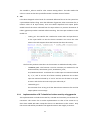
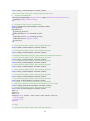
The tool also provides a push button to display the result of the dump file.
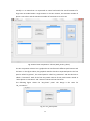
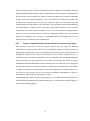
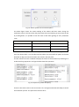
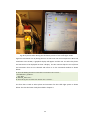
The following picture shows how the newly R-T-monitor system help to display and control
the status of the Real-Time simulation of a traffic light signal on a single monitor.
Fig. IV. Sample picture of the newly implemented R-T monitor system
1.3
Adaptations
The source code for the R-T-monitor are embedded inside a GPenSIM system, hence some
part of GPenSIM source code are added to this paper with proper citations. Also for testing
the R-T system, the idea of modelling traffic light signal using NXT are taken from the
course, discrete simulation and performance analysis with some slight modifications.
1.4
-
Chapters review
Chapter 1 is about the introduction of the thesis work, motivation, adaptation and the
statement of problems.
-
Chapter 2 is about the background of the project work idea. I.e. it briefly describe the
definition and types of simulation and modelling with some examples, and also the
need to use them in modern life. It also discusses about modelling a discrete event
dynamic systems, basic Petri net theory, and GPenSIM.
-
Chapter 3 is about the Real-Time simulation and modelling of Real-Time system. It
describes about different kinds of petri net modelling in R-T GPenSIM. This chapter also
has example of modelling real-time P-N model. I.e. Petri net in industrial application, in
6
house security, door alarm using NXT and Traffic signal system using NXT intelligent
Brick.
-
Chapter 4 is about the designing a Real-Time monitor, R-T monitors, for GPenSIM. It
describes how the design was done and also describes about a MATLAB GUIDE, a tool
that the R-T monitor were designed and implemented.
-
Chapter 5 is about the implementation of the thesis work. It deeply describes every
steps that were taken to implement the system with some code snippets and
flowcharts.
-
Chapter 6 is the testing results of the simulation and modeling of systems in chapter 3
and displaying their live real-time simulation of on the new implemented R-T monitor
interface, HCI.
-
Chapter 7 is discusses about the general methods and approaches that were taken to
implement the system, also discusses about the drawbacks of the newly implanted
system and suggests further improvement about the system. Finally this chapter
concludes the thesis work in few paragraphs.
7
Chapter 2
2. Background
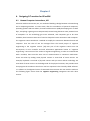
2.1 Systems, modelling and simulation
Simulation and modelling have been applied in a wide range of areas like applied science,
social science and engineering ranging from economic forecast up to space shuttle design.
Modelling and simulation are two symbiotic terms in the computing world where one of
them follows the other by a logical coincidence. Modelling is a process of creating and
presenting a mathematical symbol or formula that resemble the actual real life system by
gathering and analysing all the necessary information about how the system behaves
without actually testing it in real life, i.e. a model is a representation of the construction
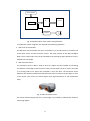
and working of some system of interest [4]. The following picture shows how to model a
system.
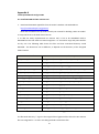
The three basic things that we should consider while we work with simulation and
modelling are:-
System
Modelling
Simulate
Analysis
Fig.1. Relation between System and M&S
System: A system is a group of objects that are interconnected in some form of logical
interaction to accomplish some purpose.
Model: Constructing a conceptual framework that describes a real system. [4]
Simulation: Perform experiments using computer by different implementation tools of the
model.
Analysis: make conclusions from the output that assist in decision making process.
As it can be seen, systems, models, simulation and analysis have some interaction. And
their interaction can be categorized in a hierarchical order as show below. [5]
8
Experiment with
actual system
System
Physical model
Experiment with a
model of the actual
system
Analytical solution
Mathematical
model
Simulatoin
Fig. 2. Hierarchy of modelling and simulating a system
An example of modelling is a reservoir model in the oil and gas industry. The engineers use
a computer program to model the actual system in order to estimate the potential of their
reservoir capacity. And also they would get accurate performance predictions for
hydrocarbon content. Besides the risk analyst can also use some simulated data in order to
analyses the risk and genuinely manage it. [6] In oil and gas industry, the mobility can be
defined by lambda. This 𝜆 Is defined as the ratio of effective permeability of the fluid to its
viscosity. For example if there is a fluid i. The mobility 𝜆𝑖 is defined as 𝜆𝑖 =
𝑘𝑖⁄
𝜇𝑖 . A
mobility ratio is a ratio of the mobility of the displacing phase to the mobility of the
displaced phase. [7] The following mathematical modelling shows the mobility ratio of oil in
an oil reservoir.
𝑀=
𝜇𝑜
⁄
𝜆𝑜
= 𝜇𝑤 𝑘𝑜
𝜆𝑤
⁄𝑘𝑤
Since one purpose of modelling is to enable the system analyst to predict the effect of
behavioural changes to the system. A model should be simple and easily understandable. A
good model should acquire realism and simplicity. Even if the system is very large, it should
always consider a modular approach to the whole system. This can be achieved by dividing
the whole system into subsystems and sub modules. Modular approach also acquires
optimization. [8]
Modelling can be represented mathematically using formulas or symbolically using some
figures. When we design a model, we should always realize the distributed probability
function. These help the system to have an accurate resemblance of the whole system with
some standard error.
9
Beyond designing a model, we can also add more features to the existing model in order to
make it more artificially intelligent and to add features like HCI, human machine interface.
This, along with a simulation and modelling, would result in a precise control system that
has all round features.
Systems can be analyzed based on the following criteria and can be decided in what way a
system can be modelled. [9]
Deterministic or Stochastic
It is always important to analyze whether the model contain stochastic elements
or not. If the system contains a discrete flow we can add random variables.
Randomness is always easy to add to discrete event systems, DES.
Static or Dynamic
We should also analyze the behaviors of the system. Whether it is dynamic or
static.
Continuous or Discrete
Does the system state evolve continuously or only at discrete points in time?
Continuous: Continues event dynamic system simulation. Uses classical
mechanics
Discrete: queuing, inventory, machine shop models, discrete event dynamic
system simulation. [9]
Real-Time or simulated time
Based on their event time, systems can be differentiated as Real-Time and
simulated time.
2.2 Discrete events dynamic systems (DEDS)
DEDS are one kind of systems that under goes a discrete event property. Usually they are
used to model and optimize systems with complex processes and distributed systems
where there is a discrete data flow. This can also provide capabilities for analyzing and
optimizing event-driven communication using hybrid system models, agent-based models,
state charts, and process flows. There are several tools that can be used to model and
simulate discrete event systems. Some of the tools that can be used are Automata, State
flow, and Petri nets at a higher level and so on. The lack of well structure integrity
(hierarchy) in Automata is a serious shortcoming for modeling large systems since a large
and complex system should be decomposed into sub models and systems. [10] The state
flow is a mechanism used in Simulink. MATLAB simulation tools and Simulink can also
provide tools to model and simulate DEDS, but their intension is not particularly designed
10
to simulate discrete event systems. So in every direction, the most powerful tool to model
DES is Petri Net. One of the most fascinating features of Petri net tools are functions for
exporting Petri nets to other tools and for importing nets from another tool. Besides; Petri
net provides concurrency, parallelism and synchronization. [11].
DEDS covers all aspects of discrete event flows that include theory and formal models like;
Petri-Nets, supervisory control, Min-Max-plus algebra, discrete simulations, performance
analysis, optimization, and optimal control. [12] The basic terms in discrete systems are
events, loops or cycles. Discrete event flows can be modelled using different kinds of
mathematical methods, some mathematical models that can model the discrete flow are;
A Markov chain: It is one of method that can model a discrete event flow. (I.e. it is a series
of random values) [13]. MC is a mathematical method that undergoes transitions from one
state to another on a state space. It is a random process usually characterized as memory
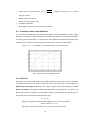
less. We can also use binomial distribution to simulate the random discrete flow. E.g. the
following figure shows a discrete flow of a simulated random numbers in some specific
time.
𝑦(𝑡) = (𝑥 + 𝑎)𝑛 = ∑
𝑛
𝑡=0
(𝑛𝑘)𝑥 𝑡 𝑎𝑛−𝑡
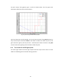
A binomial distribution function is a good explanation of discrete event flows. The result for
tasted t values is shown below.
Fig. 3. Discrete event vs time simulation
The potential of a discrete event model is described by its: [14]
•
Ability to compress time, expand time
•
Ability to control sources of variation,
11
•
∑(𝑥−𝑥̅ )2
Avoids errors in measurement, 𝑆𝐷 = √
𝑛−1
, Where x is each score, 𝑥̅ is mean
value for n terms
•
Ability to stop and review
•
Ability to restore system state
•
Facilitates replication
•
The modeler can easily control level of the details.
2.3 Continuous event time simulation
It is one kind of modelling and simulation technique used in modelling an object whose
behavior is continuous. A good example for continuous simulation is a life time simulation
of studying spontaneous flow of a liquid state. The exponential distribution function gives
continues time results of events for a given period of time. This can be denoted by
𝑦(𝑡) = 𝑒𝛾𝜋𝑡
, t=0:0.001:1, 𝛾 is constant rate, t is continuous time.
Fig. 4. Continues time simulation result
2.4 Petri Net
Petri Net is one of the widely used tools to model a discrete time event systems. A Petri Net
is a flexible tool that can be used to model any type of real life system. It is identified as a
bipartite directed graph denoted by three types of objects [15]. These objects are called
places, transitions, and directed arcs connecting places and transitions. The places are
denoted by (circles), transitions are denoted by (bars), and directed arcs denoted by an
arrow that connects the places and transitions. [31]
𝐺 = (𝑉, 𝐸)
Where V are graph vertices and E are edges or arcs in Petri net model.
V=P U T, And 𝑃 ∩ 𝑇 = 
Where P is a finite set of places and T is a finite set of transitions.
12
Token
G
Transition (T)
1
1
1
Place (P)
Arc (E)
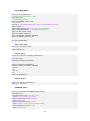
Arc Weight
Fig. 5. A simple Petri Net model with a dot token marking
Number of tokens in a petri net model can also be represented by number. The numbers
inside a small circle, places, show the total number of tokens in those places. Here note
that the numbers would be changed as a transition fires, i.e. as the event is altered.
P1
P2
2
3
2
1
T1
3
3
P3
Fig. 6. A Petri net model with number of tokens denoted by number
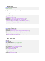
2.4.1
Places
A place in a petri net model is used as an input or output area to the model. It can
represent a buffer area, or a passive element. It is used to initialize or accept tokens. The
role of a place varied in different types of activities. Some roles of a place are list below.
[16]
•
In communication systems, a place can act as a type of communication medium, like a
telephone line, middleman, or a communication network, routers, switches, and so on.
•
It can also act as a buffer: for example, in a hard disk, conveyor belt, depot, queue or a
post bin and so on.
13
•
To denote geographical location, like a place in a warehouse, office or hospital;
•
To denote the state or the state condition: for example, the location of an elevator is,
or the condition that a specialist is available for a particular moment.
2.4.2
Transition
Transitions are event driven conditions where events are actions which take place in the
system. In a petri net, the occurrence of an event is controlled and managed by the current
state of the system. Similarly the transition has some common roles in DES. A transition can
fire only if it is enabled. A transition is enabled if the number of tokens in the input place is
greater than or equal to the arc weight. [17] A transition can be used as:
•
An event: for example, a transaction, a database search activity, starting an operation,
the death of a patient, the switching system of a traffic light.
•
Transformation of an object to another form, like accepting a product, updating a
database record, or updating a document file;
•
Transportation of objects: like transporting goods, or sending a file.
a.
Enabled Transitions
A transition 𝑡𝑗 ∈ 𝑇 in a Petri net is said to be enabled. [18]
If 𝑥(𝑝𝑖 ) ≥ 𝑤(𝑝𝑖 , 𝑡𝑗 ) for all𝑝𝑖 ∈ 𝐼(𝑡𝑗 ).
The transition t1 in figure 2 is enabled, since the numbers of tokens in the input places p1 is
2 and p2 is 3 are at least as large as the weight of the arcs connecting them to t1.
b.
Fired Transitions
As far as the transition is enabled and all the preconditions are fulfilled, the transition will
fire. Literally it means it will take a token from the input place and put it to the output
place. This also shows that an event has occurred.
2.4.3
Arcs
Arcs are connections or paths between a place and a transition or vise verse. The role of an
arc is.
•
As a Link: an arc can act as a link in communication and data transfer modelling. Simply
it is a connection.
•
As a bandwidth: - it can also act as a bandwidth in communication Medias.
•
As a work flow management. An arc in a Petri net graph can be used to model the
mechanism of workflow in industrial areas.
14
2.4.4
Arc Weight
The arc weight is the maximum capacity of the arc that can fire number of tokens at the
same time. For example if the arc weight is 2, the maximum number of tokens that can be
fired is less than or equal to 2.
2.4.5
Tokens
Tokens are input elements. Tokens can be fired to show an event has occurred and is
passed to the next part. The role of a token can also be described as:
•
Physical object, like a product, a part of a system, a manufacturing drug, a person.
•
Information objects, for example an email message, a signal, a report, a file, a packet,
a data frame.
•
Collection of objects, for example a vehicle that carries products for delivery, a
warehouse with stored parts, or an address of a file.
•
An indicator of a state, for example the indicator of the traffic signal, or the state of an
object.
A token indicates whether a certain condition is fulfilled or not. I.e. if the place contains a
token then we can conclude that the next firing state is that place by seeing the token.
2.4.6
Mathematical representation of a Petri Net
A Petri net can also be described mathematically as follow. [19]
N = [P, T, I, O]
Where:
P is the finite set of places, P = {p1, p2, p3, p4 ... pL} , where L > 0
T is the finite set of transitions, T = {t1, t2, t3 ... tm} , where m > 0
PT = , the place and transitions are disjoint properties or objects. I.e. P   is
always 0.
N  (P×T) U (T×P) is flow relationship, the Union of the relation between places and
transitions. I.e. it is the Petri net model of the set.
𝐼: 𝑃 × 𝑇 → 𝑁 , Is an input function that defines a set of directed arcs from P to T,
Where N= {0, 1, 2, 3, 4 . . .}
𝑂: 𝑇 × 𝑃 → 𝑁 , is an output function that defines a set of directed arcs from T to P.
A marked Petri net is denoted by.
(N, M0), where N is the Petri net model and M0 is the initial marking.
The initial marking is the number of token at the start of the model before
entering to a firing state. Marking µ is an assignment of tokens to the places of Petri net at
[19]
15
µ = µ1, µ2, µ3 … µn.
For example; M0 = [2 3 3] is an initial mark for Figure 6.
A Petri Net was designed to give models the specification of process synchronization,
asynchronous events, concurrent operations, and conflict or resource sharing for a variety
of manufacturing automated systems at a discrete events level. [20]
2.4.7
Firing Sequence and firing time
The firing sequence of a transition depends on different techniques. In GPenSIM When
there are more than one enabled transitions, the firing sequence is made by the
transitional definition file.
Step 1. T0 is enabled and can fire
Step 2. T1 is enabled and can fire
Step 3. T0 is enabled again after t1 fires
Fig. 7. Firing sequence
The firing time of a P-N denotes for how long the transition can fire. For example if it is 3,
the transition will fire for 3 seconds.
2.5 Extended Petri net
A pure or an ordinary Petri net, the one that has been explained so far, can be expanded to
other types of Petri net to increase the modelling performance. As mentioned above P-Ns
can be used to model a wide variety of systems. However, there may be systems which
cannot be properly modeled as P-Ns, meaning there may be limits on the modeling power
of P-Ns. [24] some of the extended Petri net are:
16
2.5.1
Timed Petri Nets
The basic Petri net models don’t have any mechanism to deal with the duration of system
activities. [21, 24, 40] But adding timing parameter to the Petri net model addresses this
issue. A deterministic times are created with transitions. This is used to achieve a better
sequence and control of the model. In this thesis, timed P-N are used.
2.5.2
Stochastic Timed Petri Nets
Stochastic time delays with transitions. A stochastic Petri net (SP-N) is a Petri net where
each transition is associated with an exponentially distributed random variable that
expresses the delay from the enabling to the firing of the transition. [22]
2.5.3
Color Petri net (CPN)
CPN is representing of tokens with different types of colors. CPN is a well-organized and
suited modelling approach for systems that consists of a number of quite different tokens
or processes that interact and synchronize. Good examples of CPN application areas are
communications, automated production control systems, distributed systems, work flow
management analysis. [20]
2.6 GPenSIM
GpenSIM is a tool for modeling and simulating the discrete event systems (DEDS). GpenSIM
is integrated inside a MATLAB platform, and thus have access to the built in MATLAB
functions. GpenSIM defines the Petri net graph in the Petri net definition files. The results
of a simulation are shown in a MATLAB file. In GpenSIM systems can be divided into
modules. These are static part and dynamic parts. The static part contains a Petri net
Definition file. If we have different modules, the pdf can be divided in two different types of
Petri net definition files. Similarly the main simulation file contains a dynamic part of a
GpenSIM. In this approach a complex systems become more transparent and can be easily
evaluated. The simulation results in GpenSIM are displayed in a text format. The main
advantage of a GpenSIM is its reduction in resource managements. The ordinary Petri net
model shows all the detail information in the frontline. But in GPenSIM the resource are
pushed to the back ground, so that one can see a clear image of the model. GpenSIM can
model and analyses any type of Petri net file. Its integration with a MATLAB environment
makes it more flexible and powerful to analyze the properties of a Petri net model. [25]
To install a GPenSIM, one must download the zipped file from the owner’s web site. The
website also provides a handy manual that makes anyone to learn fast how to use
GPenSIM. Since GPenSIM works in MATLAB platform, it must be unzipped in to the MATLAB
17
folder, or the user should set the root path inside the MATLAB file menu to GPenSIM. The
installation step is available in appendix section of this paper. After installing the GPenSIM,
the program can be tested by writing GPenSIM in the MATLAB command window.
>> GPenSIM
-------GPenSIM version 8.0; Last update: August 2013
(C) [email protected]
http://www.davidrajuh.net/gpensim
------->>
2.6.1
The Structure of GPenSIM
GPenSIM, as discussed above is a tool to model and simulate a Petri net graph. The tool
consists of two main modules and one user defined module. The two main modules are the
main simulation file (MSF), and the Petri net definition files (PDF) and the transitional
definition file as user defined module. The main simulation file consists of dynamic details
like initial markings, firing times, global variables and so on of the P-N model. GPenSIM uses
a modular approach to model a Petri net graph. The Petri net definition file consists of the
Petri net properties like set of places, set of transitions and set of arcs. [26]
The Architecture of the GPenSIM is shown below in figure 12. It shows how GPenSIM is
integrated with the MATLAB tool boxes.
PDF
MSF
Other
MATLA
Tools,
like
control
systems,
Fuzzy
logic
TDF
GpenSIM
Net Utilities
Timer
Simulator
Analysis
MATLAB Engine
Fig. The Architecture of GpenSIM
Display
Simulasjon results
Fig. 8. General Structure of GpenSIM [25]
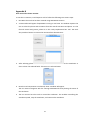
A new tool has been under construction in order to develop a graphical user interface for
GPenSIM. The new project will have a visual interface tool as shown below.
18
GPenSIM operational files
The following figure shows how GpenSIM operates to model and simulate P-N models.
Transitional definition
files, pre and post files
(Pre and post)
Matlab
Engine
Main
Simulation File
(Consists of dynamic
details) MSF
Petri net
definition
File(PDF)
Fig. 9. Basic GpenSIM Operations
2.6.2
The main simulation file (MSF file)
The main simulation file consists of dynamic codes like the initial dynamics, the initial token
states, and functions to display and control Petri net properties on the command window.
The different files (main simulation file MSF, Petri net definition files PDFs, and transition
definition files TDFs) can access and exchange global data using global variable called
global_info. [26] The ‘global_info’ can also be used to control the condition of a TDF by
semaphore. The global info variable can be accessed by the Petri net definition file, main
simulation file, and transitional definition files.
2.6.3
The Petri net definition file (PDF file)
The PDF in GPenSIM consists of the set of places, the set of transitions and the set of arcs. It
has also a set of Inhibitor arcs. The good thing with GPenSIM is it supports an inhibitor arc.
The PDF file in GPenSIM is denoted by '_def.' where the user can write the PDF name by
adding the '_def.' file where it is saved as a MATLAB file. [22, 26]
2.6.4
The transitional definition file
The transitional definition file consists of two files, these are called pre and post files. The
pre-condition consists of a user defined functions that shows an event which happens
before a firing state of the transition. In this part, we can infer different kind of rules that
controls the control activities of the simulation. Similarly the post condition consists of a
user defined functions that shows a post events, which happens after a firing state of the
transition.
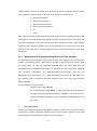
An example of a pre and post file for the above is shown below.
19
We use a COMMON_PRE file if we have transitions that have a common pre event of a
transition. On the above code, the Common pre file accepts a transition and fires according
to their sequence. Note that pre and post conditions are user defined function. Similarly for
a post condition we use a common post file.
GPenSIM also provides different kinds of Petri net analysis tools, like colored Petri net,
resource management, project scheduling, internal clock, Coverability tree, prioritizing
transitions, measuring activation time, stochastic timing, modular modelling approach and
many different optional tools to analyze and control the performance of the given Petri net
model.
Generally GPenSIM can serve from modelling and simulating up to analyzing a discrete
event system.
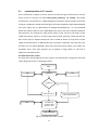
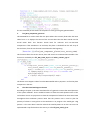
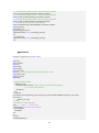
The steps used in designing a GPenSIM code are shown below:
Step1. Create the Petri net definition files, PDF, or modules.
- Identify and write the basic elements of a Petri net graph: the places,
- Identify the basic elements of a Petri net graph: the transitions, and
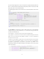
- Connecting the elements with arcs. I.e. connect the places and transition based on the PN rule. The following picture shows the structure of the pdf file. The ‘Petrinetgraph’ is a
gpensim build in command to road the pdf file from the drive. Note that we use this file in
main simulation file.
20
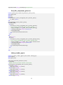
Note that ‘mypdf_def’ refers to the Petri net definition file.
Step2. Create the transitional definition files, i.e. _pre and _post files.
Step3. Create the main simulation files.
-
Identify the global variables, i.e. make some policies.
-
Load the pdf file. Using the above command:
>>png=petrinetgraph ('mypdf_def')
The png returns the set of places, set of arcs and set of transitions. If there are more than
one pdf files, i.e. modular approach. The calling will we as below.
>>png=petrinetgraph({‘mypdf1_def’,’mypdf2_def’,’
mypdf2_def’})
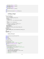
- Declare the initial dynamics. The initial marking and firing times of the simulation. Usually
the dynamic systems are denoted as ‘dyn’ in gpensim. The initial dynamics are declared as:
>>dyn.m0 = {‘p1’, 20,’p2’, 15,’p3’, 6},
Here the “m0” denotes the initial marking or the number of tokens at the starting point.
Here note that we don’t need to declare for every place in the model. I.e. we can declare
this only for places that have tokens at the beginning.
Similarly, the initial dynamics contains firing time of a transition. For example if we want
the transition to fire for 6 seconds, we can write declare the firing time as,
>>dyn.ft = {‘t1’, 6,’allothers’, 1}
“allothers” refer to the rest of transition. It serves as a default firing time.
After declaring the two cell arrays, the next step is packing them into the initial dynamics
pack. This is denoted as.
>>pni = initialdynamics (png, dyn)
21
-
Call the gpensim file. Using a ‘gpensim’ command by passing the “pni” and “dyn” struct
variables.
>>sim = gpensim (pni)
Then the ‘gpensim’ will compile the inputs and process the simulation file by calling the tdf
files and gives an output. The output file can be represented either using a plot or print
state space to print out the simulation result in ASCII code.
.
22
Chapter 3
3. Overview of Real-time simulation and some application
Time, event and cycle (loop) are key terms in simulation and modelling. Some events
occurred for a specific period of time interval and some events may occur as a cyclic event.
Thus, to simulate a model we need to define the time interval in which one event has
happened. The two types of time in simulation are simulated time and real-time. Based on
these, we can simulate any kind of model weather it is discrete or continuous. When we
consider a type of simulation and modelling, we intended to calculate the overwhelmed
time venture of the two events. In this chapter we will see different types of R-T models on
different application areas.
3.1 Real-Time simulation and modelling
Real-Time simulation and modelling exists on different application areas. It is one type of
simulation and modelling technique that is applied for different kinds of control activities in
addition to simulating systems in real-time. It can be used in both discrete and continuous
event simulations.
A simulation can be modelled using a stochastic and simulated time in order to predict
some imaginary system however when we think of Real-Time applications, the feasibility of
a real-time simulation is unquestionable.
In real-time simulation time is everything. For instance we may be interested in
guaranteeing that the nth occurrence of some event  takes place before a deadline time .
Hence the simulation time can be denoted as. [27]
𝑇𝛼,𝑛 ≤ ()
The performance measurement is denoted by: 𝑃[𝑇𝛼,𝑛 ≤ (γ)]
Similarly for discrete event time it can be expressed as:
Let Xn () denote a time interval between two events of a given type. For example
Xn () denotes nth lifetime of event , defined as the interval from the instance when  is
activated until the time it occurs and the first subsequent occurrence of another event .
Similarly we can define another event Yn (). Both event X and Y depends on the
parameter,. Finally  can be some random value. We can develop a method to calculate
their probability for [Xn () +Yn () > R] as.
𝐿𝑛 (𝜃) = 1[𝑋𝑛 (𝜃) + 𝑌𝑛 (𝜃) > (γ)]
An example of a real-time simulator is an airplane pilot simulator where the main simulator
control unit reads every sensor and actuators data live and compile it using a simulation
23
engine. Here we need to mind that one can simulate any type of model, which are suitable
for discrete event flow, using a real-time or a simulated time.
Since GPenSIM is used to simulate and model discrete event systems, the focus of the
thesis will be only the real-time in discrete event dynamic systems. Note that GPenSIM runs
both in simulation clock and real-time clock.
3.2 Real-Time Simulation using GPenSIM
GPenSIM uses two kinds of timing for timing event. It uses a real-time or simulated time.
[29] There are different kinds of tools that can be used to model and simulate systems in
real-time. MATLAB provides different kinds of tools like SimEvents and SIMULINK in order
to perform simulation. Both tools are capable of performing real-time control activities and
allow incorporation of diverse tools like fuzzy, neural net, etc. and libraries. However, these
two tools are general purpose simulation tools and are not Petri net based. [28] The need
for Petri net based simulator because of the many benefits of using Petri nets (such as
possessing simple graphical representation as well as strong linear algebraic representation
that allows mathematical analysis both on the structural and on the behavioural front) for
modelling and simulation of discrete events. LabView is another good tool that can be
defined as a real-time control simulator; however, “LabView” is not based on Petri nets
either. Generally there isn’t a single tool that is purposely designed for simulating Petri net
based with real-time capability and allows an easy integration of diverse tools and
techniques in the models of discrete event dynamic system. [29]
A real-time Petri net model consists of:
𝑅𝑇𝑃𝑁 = (𝑃 − 𝑁, 𝑆𝐸, 𝐶𝐸, 𝑇𝑖𝑚𝑒)
Terms
Description
P-N
P-N is used for graphical Petri net model, i.e. Ordinary P-N.
SE
The Extension for system resource. It is defined as SE = (R, Ω, o, t, X, Y),
R-set of system resources, R= {R1,R2, …}
Ω-set of executable operations, Ω= {a1, a2, a3, …}
o-the partitioning of the operations into subsets that can be executed by the
individual resources. o: R →2Ω
t-the set of timing that are taken for operations, t: R× Ω →N+
X, Y are input and output components.
24
CE
Stands for the Color Extension of a P-N model, it functions as
- overloading tokens with some data to differentiate one token from another
- map transitions to logic functions
Time
Time=[PTime,TTime],
TTime : Set of transition time, i.e. firing time, it is the time taken by transitions
to fire. Firing time can deterministic or stochastic.
PTime: The time taken by places to hold a token. Holding time can deterministic
or stochastic. [29]
Table. 1. Real-Time Petri net components
According to GPenSIM formalism, the design issue of a real-time in GPenSIM considers
three main design approaches. These are:
-
Realizing ‘token game’ in gpensim structure: by a method like ‘as soon as
possible, ASAP firing’, ‘delayed firing’, or by ‘aging’.
-
Realize a way to model events: Consider the options; either events by
places or event by transitions.
-
Analyze a way to interact with the external environment of the model: Is
it either thorough ‘places’ or by ‘transition’.
A token game in GpenSIM is defined as consumption of input tokens and creation of output
tokens within a specific range of firing time.
The following figure shows firing time, t=n, for a token game.
Fig. 10. Token gaming
The above figure shows that at time t=0, t0 is enabled as the input place has enough
tokens to be consumed and ready to fire. Between the given firing time n, the amount of
token that are equal to the arc weight, bandwidth, will be fired in to the output place p1.
Token gaming simply shows the condition of disappearance and reemerging of tokens by
the transition.
25
3.2.1
Real-Time simulation in Industrial application
The demand of real-time modelling and simulation in industrial are steadily increasing.
Different companies prefer to have a model and simulate it before starting to plant a
machine. Even more companies prefer to do more than just modelling, simulating and
analysis. They added different features to control the simulation in real-time, i.e. they do
the simulation in real-time. A good example is a workflow modelling of CNC machine using
Petri net. A workflow model can be simulated using a Petri net. We can consider an
example of a machine control from CNC and feeds to different robots.
The actual model is
Outputs_1
Input
Production
Line
Outputs_2
Outputs_3
Overall Output
Fig. 11. Real life model of Production line
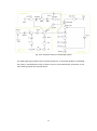
From the above real life model, we can induce a P-N model of the production facility is
shown below.
Fig. 12. P-N model for production line
26
As we can see on the above Petri net model, the system has three production lines where
all of them have the same input source. The three transitions, tProduction_line1,
tProduction_line2, and tProduction_line3 have different methods to choose color tokens
from the input. Based on the preconditions of the production line, every production line
uses different kinds of rules to fire an input token. Assume a color P-N to identify the
tokens to each production line. The tokens are denoted by different colors say ‘A’, ‘B’, ‘C’,
or ‘D’ and are used rotationally and the ‘tInPut’ generates those tokens and stored in
‘pInput_Buff’. The implementation part will be clearly described on chapter 5. Section 5.2.1
3.2.2
Real-Time simulation in room security
As it is mentioned above, we can simulate any kind of discrete event flow using Petri net
hence GPenSIM. In this part, modelling for the usual entrance gate security system will also
emphasize the concept of real-time modelling using GPenSIM. The model for such system is
available at. [41]
Fig. 13. Entrance handle with keypad
The real life model of an alarm system using three modules is shown below.
Outside
house
Security Keypad
D
O
O
R
Inside
house
Detect
Fig. 14. Actual model of a house alarm system with keypad
27
The following algorithm will give a brief steps about the working principle of an alarm
system.
The algorithm
•
If the alarm is on and ready to detect
o
Check if the entrance is ready and closed,

When opened, read and save the current time 1.


Enter the combination password within 120 second (2 min).
If the entry code is not entered within the current real-time, 1+2min, or
if the entered code mismatches with the stored codes. (after three trials)


•
•
Trigger the alarm signal.
If code is correct, keep on the cycle.
To disarm the alarm and stop the ringing tone
o
Enter the combination code in the keypad.
o
Else continue ringing.
To trigger the alarm again, store the next time 2
o
Enter the ‘exist_combination’ code. The entrance alarm will be armed after some
delay at time 2, so that the new time will be the current time.
The time interval with every firing will be
∆𝛿 = 𝛿2 − 𝛿1
We can use time P-N to define the behavior of the above model, the basic sub modules
for the above are.
Entrance door model
For a simple door model, it can be started by designing a model without a condition to
check if the door was already opened. It is because of the fact that the door might be
opened and it should be rechecked the existing door.
Fig. 15. Simple door model using Petri net
28
The above model checks only the status of the door. Weather it is opened or not, to make
it more intelligent, The door model can be redesigned as shown below by adding a feature
to check if the door is already opened or not.
Fig. 16. Door condition model with previously opened door status
The Petri net definition file for a door model will be.
Alarm model
The alarm model consists of three places and four transitions. After opening the door, if
the person didn’t enter the correct code within a given range of time, t, the alarm will
start ringing. This is only if the alarm is set to ‘Armed’. If the alarm is not set or ‘disarmed’,
it will be off or needs to be armed otherwise anybody can enter to the house.
Fig. 17. Alarm model using P-N
The Petri net definition file using GPenSIM for the above model is shown below
29
Keypad model
The keypad has two transitions each of them with two transitions to fire from an idle
token event that has been stored inside the ‘pBuffer’ place. The ‘tExit’ generates a token
that armed the alarm.
Fig. 18. Model of keypad
The Petri net model for the above system is shown below.
The overall model
The combined system model will look like as follow. There are three modules, and in the
picture below the blue highlighted border color show the sub models of the whole
system.
Fig. 19 The overall alarm system model
30
Now the above model is a simple model, to make it more intelligent we can add a sensor
instead of the combination and wait time. Section 3.3.2 introduces a method by adding a
sensor and NXT device.
3.3
Real-Time simulation and modelling using NXT machine
3.3.1 NXT Mindstrom device.
The NXT Mindstrom is a multipurpose microcontroller device that has multi functionality.
The device can be used to model robots, traffic lights, material sorting, and different types
of sensor based systems. The NXT device components can be bought in a form of a pack.
The packs contain different types of equipment that are used for educational purpose. In
addition to the main microcontroller unit (NXT brick) there are different cables, building
Lego bricks, different sensors like; ultrasonic, light sensor, sound sensor, tough input
sensor, light lamps, and small tires if someone wants to build a simple robot or vehicle and
so on. [38]
The main components are:a. Hardware
–
NXT intelligent brick microcontroller
Fig. 20. NXT intelligent brick [43]
This device is the main microcontroller unit and it has a firmware which can be integrated
with many platforms (open source) and can be coded by different programming languages.
The NXT brick contains ports to take input and output, processor unit, memory, Bluetooth
card, LCD display.
•
Main processor: Atmel® 32-bit ARM® processor, AT91SAM7S256
•
256 KB FLASH, 64 KB RAM,48 MHz
•
Bluetooth wireless communication CSR BlueCoreTM 4 v2.0 +EDR
System
•
USB 2.0 communication Full speed port (12 Mbit/s)
31
–
–
•
Four input port, three output port, 6-wirecables
•
100 x 64 pixel LCD graphical display
•
Ultrasonic sensor
•
Sound sensor
•
Touch input sensor
•
Light sensor
Sensors
Connecting Cables
•
–
USB cable
Building bricks
•
Different kind of Lego building bricks to build the support.
This are taken from LEGO toys.
•
Software
•
RWTH- Mindstrom.
•
Fantom driver.
•
NeXttool
3.3.2 Door alarm system using NXT
A door alarm system can be modeled using NXT intelligent Brick and GPenSIM based on a
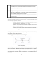
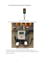
predesigned Petri net model. The following shows a clear image of the model concept.
Fig. 21. A door alarm model using NXT and ultrasonic sensor
The real life model of the above picture is shown below.
32
Alarm Switch
Outside house
DOO
R
Inside
house
NXT
Detect
Fig. 22. Model of door alarm system using flowchart
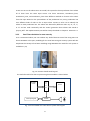
To model the system using NXT, we required the following equipment.
1. NXT brick microcontroller
The NXT brick microcontroller has port to interface to PC and also ports to interface the
touch input sensor and the ultrasonic sensor. The main purpose of the NXT intelligent
Brick is that is takes input from the PC and detects the passing by object based on the predefined Petri net model.
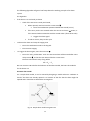
2. NXT ultrasonic sensor
The ultrasonic sensor in NXT is used to sense any object and also capable of calculating
the distance of the object from the sensor node. The ultrasonic sensor is used in this code
as a sensing node of an object who intended to cross the door. The ultrasonic sensor
Measures the distance between the NXT Ultrasonic Sensor and the nearest object in front
of the sensor. The sensor can detect objects from approximately 5 to 255 centimeters
away.
Fig. 23. NXT Ultrasonic sensor
The sensor detects objects that are in some angle. It is possible to calibrate the ultrasonic
measuring degree.
33
Fig. 24. Angular range of ultrasonic sensor detection
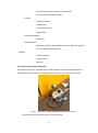
3. Touch input sensor.
This input button is used to reset the alarm. It restarts the operation of the alarm
system. The NXT touch input sensor works when a user presses the orange button. The
NXT brick has four input ports and read this sensor input and makes an output.
Fig. 25. Reset button, NXT touch input sensor
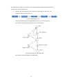
The flowchart for the alarm system is shown below
34
Object/Person
Door
No
Detect
Yes
Alarm on/off
Enter Code
Yes
?Equal
on
alarm off
trigger alarm
(NXT)
Enter
Fig. 26. Flow chart of Door alarm system using NXT
•
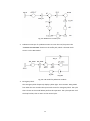
And the Petri net model for the above flow chart will be as shown below.
Fig. 27. A Petri net model of door alarm system
35
The whole system can be divided in to two modules and each of them will be called in the
main simulation file. The first module is to model the door and the second one is to model
the NXT sensor.
The static P-N of the door alarm model is shown below.
Similarly the static P-N of the NXT ultrasonic sensor is shown below.
The main simulation file and the transitional definition files are described in the
implementation section.
36
3.3.3 Traffic light system modeled using NXT intelligent Brick
Fig. 28. A Traffic light system
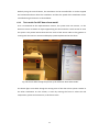
The traffic light system model designed using an NXT is shown in the following picture.
Fig. 29. Traffic light model using NXT
The following model shows a traffic light system designed using NXT and Matlab. It is the
resemblance of the above model. The model was taken from the work of Norwegian traffic light
system from UiS. [29,39]
37
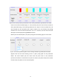
Fig. 30. Integration of Traffic signal system with GpenSIM
The model uses different kind’s components NXT components. The components that are used in
the model are list below:
-
NXT brick, the main microcontroller unit.
-
A usb 2.0 cable to connect the device with a PC.
-
Two NXT touch input sensor.
-
Three output light cables.
Fig. 31. NXT Touch button sensor
Fig. 32. A cable to connect light displays to the NXT intelligent Brick.
38
The model consists of three sub models, where each of them has different interaction with
the NXT ports. The sub-modules are;
1.
Normal cycle: This presents a normal cycle of a traffic signal in a junction. The
standard cycles of a traffic signal is:
Red
Red+yellow
Green
F
Yellow
fig. 33. Traffic lighting cycle
These are the status when the lights bubs that turns on at the same time t.
The ordinary P-N model for the above steps is shown below.
Fig. 34. P-N model for traffic light cycle
The module can be redesigned as shown below.
39
Red
Fig. 35. Module for normal cycle
2. Pedestrian interrupt: If a pedestrian want to cross the road, he presses the
“PEDESTRIAN-CROSSING” button on the traffic pole, which is the NXT touch
sensor 2 in the NXT model.
Fig. 36. P-N model for pedestrian module
3. Emergency blink:
The emergency blink frequently displays yellow light. The transition ‘tEM_START’
fires when the user touches the input touch sensor for emergency blink. The cycle
that is shown in the model below perform this operation. The cycle operates until
the loop finishes, then it return to the normal cycle.
40
Fig. 37. P-N model for emergency blink
4. The overall model is
The system uses a modular approach. All the above sub-system models’ combines to
make a complete traffic light model. The P-N model that shows the overall system is
shown below.
41
Fig. 38. A complete model of a traffic light system
The traffic light signal model consists of NXT equipment. To interface the NXT to a MATLAB
we need to install different kinds of drivers and set up the Bluetooth connection of the
main working station with the NXT device.
42
Chapter 4
4. Designing R-T monitor for GPenSIM
4.1 Human Computer Interactions, HCI
A human machine interaction, HCI, is a method of building a bridge between a human being
and a computing machine. In recent times, after the introduction of personal computers,
operating systems and text editors, the HCI tools become a rapidly developing tool. In these
days, everything is getting more computerized; Human being becomes more potential user
of computers. As the technology got more advanced, and computers get to be more
available, there becomes some sort of need to shape the human interaction with computer.
The cognitive science introduces a method to simplify the interaction between human and
computer. Thus the idea of HCI has emerged from the broad project of cognitive
engineering in the cognitive science. [30] One part of the cognitive science was the
development of some scientific and well informative applications known as "cognitive
engineering". HCI was one of the results of cognitive engineering. In order to communicate
with a machine, there must be some sort of communication or connection mechanism.
These are either by making some physical contact or some kind of sense contact. For
example, keyboard is one kind of physical contact and eye sensor and RF technology are
some kind of sense contact. At the background of the physical contacts, HCI provides tools
that program the machine to do what a user has requested. This is literally called software.
I.e. software is a background series of commands that interacts the user with the machine.
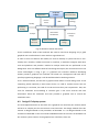
The following figure shows how the cognitive engineering categorizes HCI with other
science.
43
Computer
Science
Ergonomics
Human
Factor
Quality
Software
testing
Technical
Communication
Content
Strategy
HCI
User Experience/Usability
Information
Architecture
Analytic
s
Market
Research
Library science
Interaction
Design
Software
Design
Fig. 39. Human machine interaction
There are different kinds of HCI methods. We need to mind that designing only a good
graphical user interface doesn’t mean we have a good HCI tool.
In order to have an effective HCI model, we need to develop a system that has a userfriendly user- interface, reliable connection or interface, a method to integrate with other
tools and platforms and provide a method to analyse works that are performed at the
background. There are different kinds of interfacing techniques; the most known one in the
recent technologies is using a ‘gui’, i.e. graphical user interface. Different developing
studios provide a graphical user interface tool which has a background call back with a
specific programming language. It will be well described in the design section.
As it is discussed above, the HCI with a graphical view makes a human being closer to the
computing world. Especially in areas where there is a need to visualize events that are
performing in a real-time, the need for an HCI tool must be a prior requirement. Thus; HCI
tools for simulation and modelling in real-time give a user more accurate and clear
information about the simulation and even provides a graphical tool to control the
simulation event.
4.2 Design R-T display system
The new implemented tool in this thesis has a graphical user interface (R-T monitor) which
will serve as a display unit for the real-time control activities. The design method of the R-T
monitor is designed based on the parameters of GPenSIM. I.e. it is designed based on the
formalism of GPenSIM so that it would be embedded inside the structure of GPenSIM. The
R-T-monitor system consists of two graphical user interfaces, these are:
44
a. The main form, GUI.m, to control and display the ongoing visual display unit called GUI, this
also serve as a control unit for the real simulation system. The GUI gives all the necessary
information about the status of selected transition and places. As it is mentioned on the
statement of problems, it would be very practical if we are able to watch the transition of
every live event. This gives GPenSIM a full HCI tool.
b. A window to select the desired transitions and places, select_R-T_monitor.m, from the
overall ongoing simulation components, i.e. places and transitions.
On the monitor, the reason that a user need to select some specific transitions and places is
that when we work will a large systems, it is impractical to control all the conditions of the
transitions and places simultaneously. GPenSIM is well known by its efficiency in modelling
discrete systems that use a Petri net tool. Or simply it is a general purpose Petri net tool.
AS it is mentioned above, the R-T monitor source code is embedded inside GPenSIM. The
algorithm of an extended GPenSIM is shown below.
The over view of the GUI in the system is
Matlab
HCI
Using
MATLAB and
MATLAB
GUIDE
Transitional
definition
Matlab
Engine
files, pre and post files
(Pre and post)
Main
Simulation File
(Consists of dynamic
details) MSF
Petri net
definition
File(PDF)
GpenSIM Structure
Fig. 40. The over view of R-T monitor
4.3 User interfaces design
Though GpenSIM can model and simulate any type of Petri net model, it lacks a mechanism
to have a graphical human machine interface, HCI tool. This tool is a system that makes the
user to have a visual interaction with the background resources. GUI tools provide a
method or class object called FORMs which has components like textboxes that are visible
for humans. A user can easily interact with pre designed forms. The forms for graphical user
interface are designed using MATLAB.
Here we should mind that we can use another tool to implement the GUI. The design of a
GUI is very complicated and tricky unless a careful design approach is taken. Here in this
45
thesis project, i intended to use a MATLAB GUI designer called GUIDE for implementation. It
is obvious that most developing software platforms provide a tool to implement a graphical
user interface. This is due to the rapid development of HCI. Based on this it has been taken
some assessments on using different tools like java and visual studio.NET. But the better
method to design a graphical user interface component for GPenSIM is GUIDE. MATLAB
provide a tool for designing graphical user interface called GUIDE and the associated file
extension is called ‘.fig’ For example; GUI.fig. [32]
4.3.1
Graphical user interface (gui) basics.
Graphical user interface tools are tools that make a visual and graphical human machine
interaction. Now a day’s most software provides an efficient graphical tool to make the
user more comfortable. Every GUI tools provide a method or class object called FORMs. I.e.
A form is a class that its member functions are accessible throughout the class. All controls
in the function are objects. In java and visual studio tools, a graphical user interface is called
form, ‘jForm’ or ‘Form’. But in MATLAB, it is called figure. The figures in MATLAB GUIDE are
usually denoted as ‘gcf’.
Forms are a graphical
user
interface tools
through
which a
user interacts with the
background source code. To make the system more useful and user friendly, the interface
should have suitable controls for getting input data from the user. A MATLAB ‘gui’ form is
called figure. As it is know that all MATLAB plots are named as figure1, figure2 and so on.
This will be explained on the next section. A well designed gui should fulfil the following
three criteria. [33]
Simplicity: should have unity, elegance and clarity.
Consistency: should have a good alignment, integrity with the back code and harmony.
Familiarity: It should be user friendly and charm.
4.3.2
MATLAB GUIDE
A MATLAB gui, is called GUIDE. It is an event driven programming tool developed by
MATLAB in order to provide the users with a graphical user interface, GUI, development
environment. [34] The GUI should behave in an understandable and predictable manner, so
that a user knows what to expect when he or she performs an action. For example, when a
mouse click occurs on a pushbutton, the GUI should initiate the action described on the
label of the button. A MATLAB Guide has a lot of similarities with java applet. But MATLAB
is a bit terrible. The advantage of using MATLAB guide over using java is that it contains
libraries that perform functions needed for scientific computing. This is unquestionable.
Most engineering and scientific areas prefer to use MATLAB languages; this is due to their
46
flexibility and integrity with other MATLAB libraries. But still MATLAB has some weaknesses
like it is only useable in math Works environment. It is like it has pros and cons. The other
con is that MATLAB is very expensive software, these has been a headache for most of
developers. [32]

There are two ways of developing a graphical user interface in MATLAB. These are:
a. Using a MATLAB command ‘UiControl ‘
The MATLAB Uicontrol creates a user interface, and returns a handle of the user interface
component. For example if we want to create a pushbutton with its ‘callback’ function,
’pushbutton1_Callback’, we can the command using ‘Uicontrol’ as below.
> h = uicontrol ('Style','pushbutton','Callback', @
pushbutton1_Callback);
h can be used to return the result so that it can be used with another function.
b. Using a toolbox called GUIDE
A MATLAB GUIDE is a MATLAB toolbox used to create a graphical user interface based on a
MATLAB script file. A guide has a structure as shown below.
Matlab Root
Figure
Uicontrol
Axes
Uimenu
Push button
Image
File
Edit box
Line
Edit
Static text
Surface
Help
Uitable
Plot
Uislider
Fig. 41. MATLAB GUIDE tool components
For working with a large system, the best way to work with a gui is a GUIDE. Because GUIDE
by itself would minimize the mess by creating all call events and gives also a template. The
three main components for MATLAB gui are:a. Component or object: Objects like Pushbutton, listbox, uitable, textbox and so on. Guide
provides an easy drag and drop method in order to create a desired GUI component.
Fig. 42 Example of a component
47
b. Figures
Figures are window-forms in MATLAB. Any visual studio tool has form designer and in
MATLAB these forms are called figures. In the normal MATLAB operation, figures are
created automatically whenever the MATLAB plot function plots a data. Empty figures can
also be created with the function ‘figure ()’ on the command window. It can also be used
to plot any kind of gui components by adding the function arguments.
Fig. 43. GPenSIM file Operation figure (Created for illustration)
c. Property inspector:
The MATLAB GUIDE provides a property inspector tool. From where we can inspect
properties like background colour, component name and handle events. Almost every
GUI providing software studios have a property inspector. The MATLAB GUIDE property
inspector is shown below.
Fig 44. MATLAB GUI designer property window
48
d. Callbacks
Finally, there must be some way to perform an action if a user clicks a mouse on a button
or types information on a keyboard. A mouse click or a key press is an event, and the
MATLAB program must respond to each event if the program is to perform its function.
Every ‘callback’ function has a variable called ‘handles’ to handle each operation since the
guide is an event driven program. Generally ‘callback’ function controls the behaviour of
the gui figure and of individual components. MATLAB software calls a ‘callback’ in
response to a particular event for a component or for the figure itself. [35]
The ‘callback’s are automatically created as the user selects tools and draws on the design
layout tool. The ‘callback’s in any figure can be accessed by right click on the component
on the designer view. Note that the method ‘callback’ is the main connector of the figure
and the background program. Whenever some event happens, the ‘callbacks’ pass
arguments to the three variables.
Fig. 45. A MATLAB GUIDE designer view
For example a ‘callback’ function for the above pushbutton is shown below.
function pushbutton1_Callback (hObject, eventdata, handles)
% hObject handle to pushbutton3 (see GCBO)
% eventdata reserved - to be defined in a future version of
MATLAB
% handles structure with handles and user data (see GUIDATA)
The comments are created by GUIDE as an annotation for the GUI component to inform
what the variables are used for. These comments are optional and can be removed.
A MATLAB GUIDE by default creates a main function by passing two different types of
variables called 'varargin' and 'varargout'. Every ‘_Callback’ function passes at least three
types of variables. A developer can choose which one is comfortable for his code. Note
49
that each of them have different purposes. These are; hObject, eventdata and handles. If
each of them is not used in the ‘callback’ function the guide will put an underline warning
sign on each of them.
hObject: This variable handles the event of current operating object or component which
creates a ‘getcallbackobject’ called GCBO. In MATLAB, the GCBO are dynamically created
each time when a callback is executed. Their functionality is to get handle to current
callback object [OBJECT, FIGURE] = GCBO and returns the handle of the object whose
callback is currently executing and also the figure containing that object. [36]
eventdata: The event data in MATLAB take event handlings data and pass throughout the
platform. These are reserved for future version of MATLAB.
handles: This method is the basic for MATLAB GUI events. When MATLAB creates a
graphics object or component, it assigns an identifier to the object. [37] This identifier is
called ‘handle’ and sometimes denoted as ‘h’. One can use the “handle” identifier variable
to access the “hObject” properties with two built in functions called “set” and “get”
functions. For example, the following quadratic statements create a graph and return an
event data to a plot result object in a form of h:
𝑥 = 0: 0.1: 1
𝑦 = 2𝑥 2 + 𝑥
ℎ = 𝑝𝑙𝑜𝑡(𝑥, 𝑦)
We can use the handle event handler h to set and get the properties of the ‘quadratic
plot’ object. For example, we can set its fore ground colour property as:
Set (h,'Color','red')
We can also specify the properties when we call the plotting function in another M-script
file:
h = plot(x, y,'Color','red');
We can also get the object property by using a get function. And it will return the object
and its possible values as numerical value which is an id for that component and its
property.
A= get (gcf,’Color’), where gcf returns the current figure,
and it stands for get current figure.
Will return
ans=
0.2 0.2 0.1
This value is the combination of one of the MATLAB colour RGB.
50

In addition to the ‘Callback’ function, a MATLAB GUIDE also creates four types of
functions with some templates.
These are:
1. Guiname
This is main function and created with some templates like struct. It will be discussed in
detail in the implementation part.
The main functions with two variables look like this
function varargout = guiname(varargin)
2. Guiname_OpenFcn
The prefix “guiname” before the underline score is the name of the figure and the suffix
after the underscore is a built in function name for opening the figure file on run time.
The function is used to open the figure just after the main function is run and it fills the
‘handles.output’ with proper arguments and a starting event. The function takes four
arguments i.e. hObject, eventdata, handles and varargin.
3. Guiname_Output
Similarly the prefix “guiname” before the underline score is the name of the figure and
the suffix after the underscore is a built in function name for guide. The rest of the string
“_OutputFcn” is a reserved word to export the event data.
4. Componentname_Create
This function is created for every created component by gui. For example; if we create a
pushbutton using a GUIDE. The GUIDE will automatically create a source code for the
component to be created. Changing this function will make the component unresponsive.
4.4 R-T monitor user interfaces
The Real-Time display interface consists of three forms, each of the interfaces are invoked
by GPenSIM according to their usage. A MATLAB provides a method to exchange GUI data
in an object format.
4.4.1
Design of an interface to select a Real-Time places and transitions
The name ‘Real_PTtime_select’, which refers to Real Places and Transitions select, and is
given because this graphical user interface is used to select real-time component, here in
our case places and transitions of the Petri net definition files. This is to mean that we can
specifically select the places and transitions from over all components of the real-time Petri
net model. The need to minimize the number of places and transitions is that when we
work with large systems and while there are plenty number of places and transitions in the
model, we need to limit our focus only with some places and transitions at the same time.
51
Literally it is to mean that it is impractical to control and watch the overall activities of a
large Petri net model within a single monitor. In this R-T monitor, the maximum number of
places is set to be 7 and the maximum number of transitions is set to be 10.
Fig. 46. Real-Time components’ selector (Real_PTtime_select)
The R-T component selector has a graphical user interface with different push buttons and
list boxes. In the figure above, the graphical interface has three separated panels. The first
panel is called “RT_Places”, the second panel is called “RT_transitions” and the third one is
called a “command”. Each of the first two panels consists of two push buttons named as
“select places or transitions” and “remove” buttons and two list boxes.
The following figure shows the “RT_Places” panel. The design is the same for
“RT_Transitions”.
Fig. 47. R-T_places panel.
52
The first side, left side, list boxes automatically load all places and transitions from the
global GPenSIM variables and by using the middle buttons; we can choose a selective places
and transitions that we wanted to observe visually throughout the real-time simulation
process. This has also been designed to have a remove button so that we can remove the
unwanted but selected items so that the simulation won’t be interrupted. The last
command panel has two buttons “ok” and “clear”. The ‘ok’ button saves the selected items
from both panels, R-T_places and R-T_Transitions, right sided list boxes to set of real-time
components and return to the simulation process. This user interface is implemented in
aiming the user can easily select the real-time components easily from every modules
without any ambiguity. The interface is embedded inside the GPenSIM tool and run
whenever we start running a main simulation file.
4.4.2
Design of a graphical display system for Real-Time Monitor (GUI main)
This HCI form is the heart of the R-T monitor display. After we select the real-time
component using ‘Real_PTtime_select’ form, this graphical display form appears and starts
displaying the background process of the GPenSIM simulation process. The display unit is
designed to acquire all the necessary information of the real-time component. As it is
mentioned in the statement of problems, the main objective is to provide GPenSIM with
Real-Time display unit that would show the simulation of the Petri net model. The GUI is
embedded inside GPenSIM. When a main simulation file runs, it will also start running after
we select the necessary R-T monitor elements. We know that GPenSIM runs in two modes,
i.e. either in real-time or simulated time. So the GUI is designed to run in both modes, i.e. It
runs both in the real-time and the non-real-time simulation modelling but it gives an
information in what mode is the simulation running.
The following figure shows the whole GUI display unit. It has different kinds of components.
The detail will be explained in the implementation part. To illustrate the interface design, as
shown in the following figures,
53
54
Fig 48 R-T monitor main window
The components of the R-T monitor are grouped in different panels. This gives clear
information about the status of R-T elements and can easily be controlled. As shown on
fig., there are seven panels. These are:
i. Transition panel
As the name implies, this panel consists of the selected elements of the real-time P-N
model transitions. It contains detail information of every single transition. Here we need
to remember that the panel consists of only the selected transitions.
Fig. 49. Transition panel on R-T monitor
The information provided by this panel are; event display or color based animation,
associated transition names, Transitions’ status and the current time for real-time display.
The event display displays the status of every transition in the R-T monitor. Every
transition has a display denoted by a rectangle and their status is identified by different
colors based on their events. i.e., In a Petri net model, a transition has basic four states,
and these are:
a. Enable or not enabled state
In the R-T monitor the enabled transitions are denoted by green rectangle, i.e.
whenever a transition fulfils the ‘enable’ criteria in the precedence matrix in the
current simulation loop of GPenSIM, The display rectangle will switch the color to
green.
Fig. 50 a transition of R-T monitor on enabled status, Enabled transition
b. Fire or not fired state
Similarly for a transition that is currently firing in the current time and current loop,
the rectangle will be switched to red to inform the current status of the transition and
it will stay red until the next event comes.
55
Fig. 51 a transition on firing status
c. Never firing state or dead locked and enable but not firing
This transitional event status display is a little bit different. From the incidence matrix of
the Petri net, a transition can fall in to two categories. These are a transition cannot fire
in the current loop and a transition is enabled but is not firing in the current loop. This
should be observed while we work with real-time simulation. It’s because of the fact
that we can see the where about of every token and in the preconditions. If a transition
fall in this group, the color of the rectangle will switch to cyan for enabled but not firing
and light purple for never firing. Here we need to mind that the two events are alike
even if the transition is cannot fire in both cases.
Fig. 52. Never fired transitional event
Fig. 53. Enabled but not firing transition
d. Firing complete state
In GPenSIM, after a transition has passed through enabling and firing events, it will be
considered as a complete event. So in the R-T monitor, it is denoted by a yellow
rectangle as shown in the figure below.
Fig. 54. A Firing complete event
The “Transition panel” also contains information under the rectangles like caption for
the name of every transitions named as “Transition name”, colored texts based on their
status as transition status, and the current time which is in real-time. The need for a
color text is that, the events of the transition are as fast as a human eye can’t even see it
especially in sensor networks. Thus, the good way to keep an eye open is to give extra
information about an event and put it to a log file so that the user can revise it at any
time.
56
Fig. 55. Transition names, event status and Current time display
ii. Places panel
A place panel contains a similar to above section i., transition panel, and gives
information about the status of the selected real-time places of R-T monitor. Like
transitions denoted by a rectangle in “Transition panel”, places are also denoted by
small circles in this panel, this is also to give extra visibility for places. The following
figure shows the place panels in the R-T monitor.
Fig. 56. R-T monitor places
This panel also provides information about the quantity of the tokens, starting from the
initial markings up to the final token absorption in every place. When every time a
transition fires a token, the R-T monitor also displays the number of tokens mobilized in
every places inside the circle.
It has also a textbox to display which transition has taken the token and at what time.
Displaying such information is quite feasible especially while we work with some realtime simulation, controlling the movement of tokens gives extra information for the
controller. For example while modelling and simulating a building with full of distributed
sensor networks, controlling only the events might not be enough. I.e. there might be a
need to visualize the movement of every single token in every place.
57
Fig. 57. A Single place and full info for R-T monitor.
iii. Enable sequence log.
This GUI panel contains a wide textbox to display the status of the enabled transitions in
the entire simulation loop in a sequence fashion. It can also serve as a text log file and it
can be exported to another use. Note that this log stores not only the selected R-T
monitor transitions but also all the global transitions of the simulation. This helps to give
a clear image of the sequence.
Fig. 58. Enable sequence on R-T monitor screen
iv. Firing sequence log.
Similar to the enable sequence log, there is also a method called firing sequence log for
firing transitions. This again stores the entire firing sequence of the transitions.
58
Fig. 59.a Firing sequence on the R-T monitor
The space shows the loop interval and the active transition in every loop. In the
GPenSIM main simulation file, if the “global_info.PRINT_LOOP_NUMBER = 1”, the
spaces would be replaced with a string with loop number to show the loop interval as
shown below.
Fig. 59.b Firing sequence with loop number
v. Basic info
This GUI panel shows a basic info about the total number of places, transitions,
simulation name, and total elapsed time.
Fig. 60. Basic info about the Model simulation.
vi. Commands
This is also another panel that contains some commands to control the simulation, this
gives the R-T monitor extra capability in controlling the simulation besides displaying the
events. For example while we simulate a robot that takes from the CNC machine and put
59
to the buffer, if the user needs some diagnosis, the simulation can be stopped so that
the working machines also paused.
Fig. 61. Control buttons on R-T monitor
While the simulation is pause, there is some added time to the overall elapsed time, this
should be handled, otherwise in real-time simulation, delay has a significant factor. Let’s
denote a delay between two event a and b, as t
Even a
Event b
t’
Event b’
t’’
Fig. 62. Event diagram with time
Event b was supposed to happen at t’ but due to the delay t it ended at t’’. The overall
elapsed time would be, t’ + t’’, and the delay is t=t’’- t’. From this we can conclude that
pausing the simulation for longer time will make the t to be high. This can lead the
system to be less accurate.
Similarly the command panel contains a method to control the speed of the simulation,
In GpenSIM, while working with real-time, we can also speed up or delay the firing
without losing the real-time but just only adding some delay time, .
=f - o, where f is final time, o is initial time.
The difference between this and the above pause is that the delay time is very small, the
maximum 0.25, in speed control so that it won’t affect the real-time.
60
vii. Sequence display of global transition status
The R-T monitor has also an extra display to show the status of the rest of other
transitions, this would give a full functionality for the R-T monitor in displaying every
event in the entire simulation. For example in the figure below, tRobot3 may be in the
in the R-T monitor or not but it is a transition in the entire simulation.
Fig. 63. A small display panel to show the status of all the transitions in the simulation.
61
Chapter 5
5. Implementation
The R-T display system was implemented using MATLAB software. As it was mentioned in
chapter 4, The R-T monitor can be implemented with different kinds of tools like java or
other graphical user interface supporting tools like visual studio.net. Note that MATLAB
can support and access the packages of java and other languages. But the precise way of
implementing this graphics display system, or R-T monitor, for GPenSIM would be using
the MATLAB studio. This is due to the fact that GPenSIM by itself runs in a MATLAB
platform and also the performance of a MATLAB would decrease while working with an
imported graphics data especially for simulation. The previous chapter shows how the
basic interface design of R-T monitor is made and what are every single terms in the R-T
monitor. Once the system has been designed, the next math is connecting every graphical
interface components based on the GPenSIM events. During the simulation process, they
should be handling events and giving the interface a real meaning. As discussed above,
the MATLAB guide has objects like push button, textboxes, axes and list boxes and their
event driven callbacks like handles, hObject and eventdata to export and import
information. The implementation has global variables. But the following table shows the
most important global variables that carries data throughout the system. There are also
other kinds of global variables and they are added in the appendix part of the report.
Global
variables
Descriptions
Examples used
global hn
It is used to search the hObject in the gui
components.
Section 5.1.3
global PN
It is a gpesim global struct variable that
contains a every information of the Petri
net model
It makes the other classes to access the
gui event handlers throughout the
system.
This is an important gpensim global
variable, its main functionality is to carry
information of different cell arrays
throughout the system.
To store the enabling and firing
sequences to plot on R-T monitor
Section 5.1.2
global
handles
global
global_info
Global
temp1,temp2
Table. 2. Global variables
62
Section 5.1.2
Global_info in any main
simulation files.
5.1
Implementation of R-T monitor.
As it is mentioned in chapter 4, the R-T monitor has two main gui interface forms. The two
forms in the R-T monitor are called ‘Real_PTtime_select.Fig’ and ‘GUI.fig’. We should
recall that the ‘.fig’ extension is a MATLAB figure file extension which contains the layouts
of the gui components. Recall that both figure files were designed using a MATLAB GUIDE
tool. Every figure file in a MATLAB has a background MATLAB file, *.m. Thus MATLAB
keeps two separate files for every MATLAB gui file names with same name but different
file extensions. For example for ‘Real_PTtime_select’ name, there are two kinds of files
called ‘Real_PTtime_select.m’ and the layout ‘Real_PTtime_select.fig’. (Note that the two
files can be kept on separate directories, but it would be better to keep both of them
inside the same directory. A MATLAB file path can detect it wherever the other files. This
has been one pro about MATLAB). Both ‘GUI’ and ‘Real_PTtime_Select’ runs before the
simulation starts. Their main purposes are to prepare a rough sketch i.e. HCI tool to
display the simulation status.
The flow chart of R-T system
The flow chart and the algorithm of R-T monitor are shown below. The general overview
of the design was shown in the design section.
MSF
PDF
gpensim
TDF
?R-T
N
Select Ps and
Y Ts
HCI
Inform Not Realtime
Call HCI and
Continue with
gpensim cycle
Start Simulasjon
Fig. 64. The flow chart of R-T monitor
63
In the above flow chart, the HCI tool contains all the gui components and script files of the
GUI.m. The rest of the flow is a normal GPenSIM operation.
In addition to the two GUI files, the system has also different classes that help handling
the GPenSIM and filling out the information on the GUI. The functions and classes of the
R-T monitor, i.e. the GUI components and other files, are added in to the GPenSIM
background source code and these are identified by some comments from the original
gpensim file. The MATLAB scripts files that are implemented in the R-T display are:
File names
Description
Real_PTtime_select.m
See Chapter 4
GUI.m
See Chapter 4
find_GUI_component_places
To search a current source place name where a
token has been removed from GUI components.
find_GUI_component_trans
To search a current active transition name from the
GUI components.
token_number_ngt.m
This MATLAB file plots the real-time token during
the runtime.
fill_GUI_initial_dy.m
This file plots the initial marking of the real-time
places at the beginning of the simulation.
gui_painter.m
This MATLAB file has global variables like handles
which can directly access the GUI.m and GUI.fig in
Order to paint the coloured bars according to the
status of the transitions in the current cycle.
enable_AnimNGT.m
This file invokes the file ‘gui_painter.m’ with
associated transition name, current time, and type
of colour in order to paint a green bar which is
dedicated for enabled states in the R-T monitor.
fire_AnimNGT.m
Similarly this file has a function to invoke the file
“gui_painter” with variables like the transition name,
current firing time t and colour type in order to plot
a red bar for firing transitions.
fire_Complet_AnimNGT.m
This file has also a similar function like the above
two. Its purpose is to plot yellow bars for the
transitions that have completed firing with the
associated firing time t.
64
hasnotfired_AnimNGT.m
This method calls similarly the “gui_painter” file by
passing the current transitions and a flag. The flag is
used to differentiate the two states of firing of
transitions. I.e. We know that a transition might be
enabled but not fired at time t and also there can be
a condition where a transition is not enabled and
note fired at the current time t.
infoplc.m
This file has function to plot the status of the token
flowing. I.e. it will write on the GUI the starting of
the token to where the token is absorbed.
Table. 3. Implementation file names of R-T monitor.
5.1.1
Implementation of a user interface to select places and transitions.
This section is about an implementation of a figure file ‘Real_PTtime_select.fig’ in chapter
4. This figure file along with the MATLAB script file is embedded inside a GPenSIM system
directory, i.e. the guide layout file with all the graphical user interfaces components
“C:\\…\gpensim\timed_pensim\Real_PTtime_select.fig” and also the background script
MATLAB file “C:\\...\gpensim\timed_pensim\ Real_PTtime_select.m”. The use and
functionality of this MATLAB figure file were clearly described in the previous chapter. The
main function of the GUI is:
i.
The main function
In MATLAB working environment, the main function name and the file name use the same
name. For example in Real_PTtime_select, the main function and the file have the same
name. [33]
-
The file name is, ‘Real_PTtime_select.m’
-
The function name is, function varargout= Real_PTtime_select()
The main function, Real_PTtime_select(), takes two arguments, like any other figure
created by GUIDE. These are “varargout” for output and “varargin” for input variable
arguments.
Varargout - is a cell array for returning output arguments.
E.g. varargout {1} = handles.output.
Varargin - is also a cell array for passing variables as input arguments.
65
The main function begins with a series of comments for help documentation about the
GUI. I.e. if someone wants to know about the Real_PTtime_select he can just type ‘>help
Real_PTtime_select’ on the command window.
The following figure shows the main function that is created by GUIDE to start the GUI
layouts.
The ‘gui_singleton’ is a variable that is used as a flag to specify if one or more duplicated
instances of the gui can exists simultaneously. I.e. it controls how many gui windows we
can open at the same time. [32]
If ‘gui_singleton’ = 1, then there can be only one copy of the figure layout.
If ‘gui_singleton’ = 0, then there can be more than one simultaneous duplicate of the GUI
figure. So in our R-T monitor, the ‘gui_singleton’ is always 1. I.e. there is no duplicate of
the GUI at the same run time.
In addition to a ‘gui_singleton’ variable, there is also another declared structure variable,
this struct contain all the declared variables in a struct form. These are; ‘gui_filename’,
‘gui_singleton’, ‘gui_OpeningFcn’, ‘gui_OutputFcn’, ‘gui_LayoutFcn’, ‘gui_Callback’. This is
automatically created by the GUIDE environment. The purpose is just to store the GUI
state in one structure.
gui_State = struct ('gui_Name', mfilename,...
'gui_Singleton', gui_Singleton,...
'gui_OpeningFcn', @Real_PTtime_select_OpeningFcn,...
'gui_OutputFcn', @Real_PTtime_select_OutputFcn,...
'gui_LayoutFcn', [],...
'gui_Callback', []);
66
The other variables nargin, It is a MATLAB keyword used to define the number of input
arguments for the main function. So the condition
if nargin && ischar (varargin{1})
gui_State.gui_Callback = str2func (varargin{1});
end
Checks if there are input arguments i.e. ’varargin {1}’ and the inputs are of
character array. If the conditions are fulfilled, then the Callbacks will be populated inside
the gui_struct and perform a graphical layout operation.
The results will also be processed using ’nargout’. Like in the above condition for
’nargin ’, the variable ’nargout’ also checks if there are output arguments. For
example if a push button is clicked and the click has handled an event to do something.
The result should also be appeared on the graphical user interface. The condition that
checks this operation is shown below.
if nargout
[varargout{1:nargout}]= gui_mainfcn(gui_State,
varargin{:});
Else
gui_mainfcn(gui_State, varargin{:});
end
From the above condition, if nargout is true, then the main function calls the other
MATLAB function ‘gui_mainfcn’ and passes the struct gui_state and all of its input
arguments (varargin {:}) and returns as an output argument, varargout. If the there is no
output, i.e. nargout is not true, then the gui_mainfcn will be called but varargout is
null.
ii.
OpenFcn, OutputFcn and CreateFcn
a.
Real_PTtime_select_OpeningFcn
As it is mentioned in the previous chapter, whenever we create a GUI using GUIDE, a
MATLAB automatically create different functions with some templates that can be edited.
[32] The function ‘Real_PTtime_select_OpeningFcn’ is also a type of function created
while designing a ‘Real_PTtime_select_OpeningFcn’ but has been modified to fulfil the
conditions of the R-T monitor functionality. This function takes three input arguments of
‘hObject’, ‘handles’, ‘varargin’ and ‘eventdata’.
The ‘hObject’ refers to the current
component that is doing some activity or event and ‘handle’ is an event handler of the
‘hObject’. The function keeps the object for example pushbutton and put it in to the
handles structure as an output.
67
The variable ‘guidata’ pass the content of the two variables ‘hObject’, ‘handles’. This
‘guidata’ store components like hObject along with their associated events and keep them
in a form of structure data type.
This function is called only once in the R-T monitor. As mentioned above, the main
purpose of this gui form is to select some places and transitions for displaying and
monitoring.
b.
Real_PTtime_select_OutputFcn (OutputFcn)
This function returns the output data to the MATLAB command line interpreter after the
opening function returns control and before control returns to the command line
c.
CreateFcn
This function contains an event that is used to create components like push button,
dropdown menu and so on. For example a function to create components for 'listbox1' is
named as listbox3_CreateFcn. This built-in MATLAB function automatically creates the
‘edit1’ textbox.
The ‘hObject’ in the above function is used as the newly created event handling object.
And the ‘eventdata’ are reserved to the future MATLAB versions.
The variable ‘handles’ contains a structure with event handles and used to pass the newly
created object’s event.
The GUIDE always creates components with templates. For example in the above list box,
the default is created to be the window’s default background color.
iii.
The callback functions
The above functions are just used to make layouts of the gui design, These functions are
created by the GUIDE with some templates. To make the layout work the selection, their
68
callback function need to be added. Since there are six buttons in the gui interface, there
are six different ‘callback’ function for each of the buttons. The buttons are:
a. Select Places button
b. Remove places button
c. Select transitions buttons
d. Remove transitions button
e. ok
f.
Clear
Both a and c have similar callback functions. Both of them take the selected item from the
listed places and transitions from the left side list boxes and store them in to the right side
list boxes respectively. At the same time the call back functions in a and c above build a
string array that will be the global_info.rt_palces and global_info.rt_transitions. The other
function b and d are used to remove unwanted items. The ok button returns to the main
GUI display.
5.1.2 Implementation of graphical Display for Real-Time Monitor
The declaration and initialization parts of the “GUI.fig” are similar to that of the previous
section, “Real_PTtime_select” with some extra codes. Similarly this class contains both
the layout figure file and the associated MATLAB script file. These both files are
embedded inside a GPenSIM system folder, i.e. the guide layout file with all the graphical
user interfaces components “C:\\…\gpensim\timed_pensim\GUI.fig” and also the
background script MATLAB file “C:\\...\gpensim\timed_pensim\ GUI.m”. The GUI.m has
also different kinds of functions that plot constantly each event to the gui interface
display (GUI.fig).
In the GUI figure of the R-T monitor;
-
The file name is called ‘GUI.m’
-
The main function is called ‘GUI ()’, It takes and passes an input argument
‘varargin’ and return an output argument ‘varargout’. The prefix name var
is associated with the different types of variables in a MATLAB struct cell
array form.
i.
The main function
Similar to the implementation of ‘Real_PTtime_select.m’, section 5.1.1, the main function
of GUI takes variable arguments and also returns some variable arguments, the main
function with its input and output arguments is shown below:
69
This main function is also created by the MATLAB GUIDE tool as a calling function to call
the figure file components. The comments are written for documentation. I.e. it will be
served as a help file.
As it can be seen, everything in this main function except the function name is similar to
the declaration of ‘Real_PTtime_select.m’ file. Initially this function was created as a
template. i.e. It is a default ‘gcf’ control function of the MATLAB GUIDE file that creates
the basic layouts [33, 34, 35]. Then it has been edited according to out intension.
ii.
OpenFcn, OutputFcn, CreateFcn
All of the three functions have a similar structure as that of the previous section. This are
again initialized by the MATLAB GUIDE tool and edited according to the aim of the R-T
monitor. The Opening function that has been called by the main function is shown below.
This function is used to import and work event data. The keyword guidata accepts
variables of the object or components called hObject and the event handler handles. The
function will invoke another function that is called a start function by passing variables of
the input arguments ‘hObject’, ‘eventdata’ and ‘handles’. Those variables will call the
function that starts the plotting and painting.
70
Similarly to the previous one, the output function would also be initialized automatically
by the GUIDE. The main objective to prepare an output argument called ‘varargout’ that is
used by the main function. The following code snippet shows the GUI_OutputFcn. Note
that GUI is the name of the R-T monitor in the thesis.
The varargout {1} refers to the number of event handles that would be returned as an
output argument.
The ‘createFcn’, as mentioned in the previous section, is a function that creates the entire
layout for every ‘gui’ component.
iii.
Start The graphical user interface and plot the basic layouts
The function ‘GUI_OpeningFcn’, from the above section, invokes a function called
‘startCode’ which starts plotting a small circle for places and a bar for transition. Here not
that the places and transitions are the selected places and transition from the overall places
and transitions for a Real-Time displaying purpose. The function to do such condition is
shown below.
In the above code snippet, the global variables are used as a bridge to import a gpensim run
time components. Note that In MATLAB GUIDE the global variables should be declared
inside every function unlike other programming language where global variables are
declared on the top the class. [37]. in this implementation, the “global_info” is used to pass
global variables. GPenSIM stores every component in a structure called PN. This PN
contains information about the Petri net model. For example for figure 1 in the chapter 2,
the PN struct variable contains a structure that is shown in in the next figure.
71
The above figure is a PN structure for a petri net model that has three places and two
transitions. The structure value contains information like name, number of places, global
places, and set of firing times, system resources and so on. For example the name of the
simulation is denoted as PN.name, it contains the name of the simulation. Similarly it
contains the global transition and places and these are denoted as ‘PN.global_transitions’
and PN.global_places. Note that both of them contain a matrix structure. For example if we
have three places, the PN.global places will be: PN.global_places: [1x3 struct] and it will
return the name of the places, the total number of tokens in that places and the token
bank, a place where tokens are absorbed and stored. The [1x3 struct] for the above
structure give a result in the command window as:
The next step is to organize the global variables as below before moving towards to
plotting. Here the GUI accepts both the Real-Time and the non-real-time simulation. This
condition is checked as
72
–
If it is not a real-time, i.e. if we are using a simulated time, the places and
transitions are by default extracted from the global PN variable. Simply we don’t
have places and transition that are selected for real-time display purpose. I.e.
‘Real_PTtime_select’ didn’t run in the gpensim. The values are
 PN.global_places
 PN.global_transitions
–
If it is in real-time, i.e. we have places and transition that are selected on run time
from the ‘Real_PTtime_select’ interface. These values are named as:
 global_info.rt_monitor_places and
 global_info.rt_monitor_trans
After calling the global values and check whether they are the member of the real-time or
not. The next step is to pass each of those values to the MATLAB gui plotter to plot the
circles and bars.
a. To display the status of places
For the places, the plotting is done as in the following code snippet. It shows the calling of
the MATLAB ‘axes’ and ‘Edit’ gui components for every places in that cell array. The ‘axes’,
which are MATLAB gui components, are used to plot small circles to illustrate the places
and the edit boxes are used to put the name of the associated place that we need to plot.
Remember that the names are extracted from the global places.
73
The function uses a MATLAB built in function called ‘eval’ in order to invoke the callback for
the edit and ‘CreateFcn’ for axes. The ‘eval’ is an easy and fast MATLAB built in function
used to run a given value.
The MATLAB string builder produces the two strings, for example for the first iteration in the
loop, the ‘strcat’ yields,
'axes',num2str(j),'_CreateFcn(hObject, eventdata, handles);'
Gives: 'axes1_CreateFcn(hObject, eventdata, handles);'
'edit',num2str(j+2),'_Callback(hObject, eventdata, handles);'
Gives: 'edit3_Callback(hObject, eventdata, handles);'
Hence the ‘eval’ evaluates the above two strings, which has a meaning in the MATLAB GUIDE.
After evaluating the strings, or calling the callbacks, the MATLAB gui starts running the string.
–
The functions that plot a small circle using axes are shown below.
MATLAB has different techniques to plot circles. The usual approach is using a rectangle
command by changing the curve as [1, 1] which the MATLAB compiler knows this is a circle.
CenterX, CenterY is the center of the axes,
74
–
The function that writes place named just below the circles is shown below
Since we have two kinds of simulation, this check whether the simulation is in real-time or
not. The main purpose of this function is to plot place names. The command, set (handles…,
‘Visible’, ‘on’), makes the initially invisible components visible during the run time. This is
because of the fact that when the R-T monitor was designed using the designer tool, GUIDE,
the components were made to be invisible and let the simulation makes them visible
whenever they are needed.
b. To display the status of transitions
Similarly for the transition, a pushbutton is used to serve as a bar to represent the selected
transitions. Again here the ‘eval’ function is used to run the built string using ‘strcat’ with the
associated place. For example if we want to plot the first place, p1, the for loop produces a
string as
'pushbutton1_Callback (hObject, eventdata, handles);
The eval will run this callback by passing the three basic variables.
The ‘eval’ runs the string and calls the callback function to plot or prepare the rectangular
bar. The string that was built on the above code and called by the ‘eval’, starts running the
following code in order to prepare a bar for the transitions to be plotted on the GUI during
the simulation. The code runs for every transition in the R-T monitor.
75
The above code clearly shows if the simulation is in real-time, the name will be taken from
‘PN.global_places’ struct variable. Every buttons were made invisible at first. Whenever
Their ‘Callback’ is called; they will be visible and ready for color plotting.
5.1.3
Other implementations of R-T monitor
The above two implementations, i.e. in section 5.1.1 and 5.1.2, are just used to select the
Real-Time places and transitions and to prepare a graphical user interface to show the
whole Simulation process for human, or they are used as a front end to communicate the
user with the background GPenSIM libraries. The main issue is not to design a graphical
user interface, rather it is to extract the basic information from the Petri net during the
simulation process and plot those values graphically and enable the user to control the
simulation accordingly. This is in other word; the statement of our problem is resolved. The
codes that do this activity, i.e. those that connect the GUI components with the gpensim
were roughly described in the table 2. In this section, we will try to look them deeply here.
i.
Plot Number of Tokens on R-T monitor
As described shortly in table 2, the function ‘token_number_ngt’ is used to plot the
number of tokens on every selected places during the gpensim runtime. The MATLAB
file that do this activity is called token_number_ngt.m. And the associated function that
passes arguments is called ‘token_number_ngt ()’. This file is also embedded inside a
gpensim system folder and contains a method to call the gui event handler and plot the
number of tokens inside the small circles on the GUI. The file is stored in a gpensim
folder as; C:\gpensim\05-Print_and_Plot\ token_number_ngt.m.
The extracted token numbers will be sent to the GUI, on the gui design view it will be
displayed as.
This gpensim calling function of this file is called ‘markings_string’. The use of the
marking_string in gpensim is to identify the markings with a range of the matrix indices.
76
[25] This function takes two input arguments, these are the markings and the range of
the incidence matrix named as ‘range_of_indices’.
Converts token vectors (markings) into a display string, e.g. [0 1 0 3] becomes 'p2 +
3p4'.
The above condition checks if there are tokens in the gpenism matrix, if there are any, it
will build the string ‘markings_str’ which contains the number of tokens in every places
at time t. Now one the tokens are extracted, the next step is to display those tokens on
the graphical interface. This is done by the token_numner_ngt.m file and it is invoked
by passing variable as shown below.
In the above code, the curr_Place is the place that is currently holding the current
tokens. Tokens are the current tokens in every places and the marking_str is the string
that has a format to display on the command window.
'p1+ p2 + 3p4' for Matrix [1 1 0 3].
The function ‘token_number_ngt’ takes those variables and start putting the number of
tokens in every place, i.e. circles in the GUI. The first step is to find the current place on
the GUI by calling the function ‘find_GUI_component_places’ and then it starts putting
those values.
77
The set command put the tokens of the places in to the gui using the global handles.
ii.
find_GUI_component_places.m
This MATLAB file is used to look after the place where the currently fired token has been
taken from. I.e. it displays the source of the current token that has been stored into the
virtual token bank. This function checks both for real-time and non-real-time
components. If the simulation is in real-time, the place is checked from the cell array of
the real-time, from the one that we have selected at the beginning.
This function takes the current source place and returns its associated GUI member. This
function is invoked by the ‘fill_GUI_initial_dy.m’ and ‘token_number_ngt.m’.
The above cone snippet is taken from the MATLAB file and its purpose is to find the place
component in the GUI.
iii.
Plot the initial markings on the GUI
According to chapter 2, the main simulation file of a gpensim contains the initial dynamics
of the system modules. Thus it would be better to show the initial dynamics also on the
real monitor screen. Its purpose is to show the comparison of token from their initial state
throughout their simulation process. Note that the previous one is used to plot the
quantity of tokens in every place as the simulation is on progress. This would give a big
picture. I.e. the user doesn’t need to recheck the initial dynamics as on the run time. The
implemented script file that does this activity is called fill_GUI_initial_dy.m.
78
X0 is used to put the initial markings in a cell array.
The function, ‘fill_GUI_initial_dy’ takes the initial dynamics of the gpensim as an input
argument and plots it on the main gui by searching their appropriate place name on the
gui interface. The MATLAB function that searches an object on the gui is shown below.
‘imarkings’ returns the initial marking of the MSF. Then from the ‘imarkings’, the code
below extracts the number of token at the starting point.
The place will be searched on the GUI using the ‘find_GUI_component_places’ function
and returns the place id on the GUI.
Once the searched object matched the one from the global real-time places i.e. the value
of s is found in the above code snippet, the initial markings would be inserted into on the
textbox that is found on the GUI.
The above loop iterates for every places whose initial markings are declared in the main
simulation file. For example, suppose we have 5 places and the initial marking is declared
as dyn.m0 = {‘p1’, 10,’p2’, 10,’p4’, 20}, where ‘p3’ and ‘p5’ doesn’t have an initial marking,
the loop skips those places that doesn’t have an initial marking even if they are
components of the real-time simulation.
79
iv.
Color plotter on R-T monitor
This file contains methods that frequently call the GUI eventdata handlers during the
simulation process for plotting the status of the selected transitions. This MATLAB file is
called from the three files i.e. v, vi, vii, and viii of the file sections below. All of them
passes similar variables but with different kinds of information including the colour types
to plot on the GUI. This is a way how the R-T monitor differentiates the status of every
transition.
The ‘gui_painter’ function is shown below. The script file that does this activity is called
gui_painter.m.
The calling function passes the arguments as follow for enable transition.
Where t1 is the index of the current transition from the enabled transitions set, ‘g’ is a
property in MATLAB for green color, and the function takes five input arguments.
args
t1
Description
Input variables
T1 is an index that selects the current transition from the global .t1
cell array.
t_btncolr
Color for the current active transition and plotted on the GUI.
‘g’ ’r’ ’c’ ’y’
textT_str
Name of the current active transition and written on the GUI.
‘Enabled’ ’Fired’
textT_colr Color for the name of the current active transition.
Str
‘g’ ’r’ ’c’ ’y’
Status in text forms and used to give information in text. i.e. Str1,str2,str3
fired, enabled and so on
Table. 4. Variable that pass arguments to the painter
The variable ‘s_trans’ is the current transition that is on processing at real-time t. then
search the transition on the GUI and plot the appropriate info.
80
The strings with a single quotation in the above code snippet shows the names of the text
boxes in the GUI designer and the ‘gui_bar’s are the bars designed on the designer of the
MATLAB GUIDE to illustrate transitions and plot the color using series of ‘set’ commands
as shown above. As it is shown on chapter four, the transitions are designed using a push
button as a bar and their name on a text box. So what actually this function do is that; it
searches the name of the transition, which is denoted by a pushbutton and the name with
a text field, and plot colors using a set command with the appropriate properties.
v.
Display real-time activities of places on R-T monitor
This file has a function that do a similar function to that of the one which writes the
tokens I every places but this one adds features that tell at what time is the token fired
and which transition is responsible for it. It gives the output like this on the GUI. The
MATLAB script file that does this activity is called infoplc.m.
vi.
Start Firing for an enabled transition
The function that starts the firing of an enabled transition in GPenSIM is called
Firing_strat.m. The next four steps, vii viii ix and x, introduces a method to plot the status
of every transitions by calling the above file ‘gui_painter.m’. All of them are called from a
‘/gpensim/13-firing/firing_start.m’ file system folder. To describe their functionality we
need to discuss about the firing_start.m file and its functions.
81
This function is called from a gpensim file where the simulation starts, the variable EIP is a
gpensim system file that is used for creating queue Q for events in progress no that EIP is
initially 0 as there is no events in Q.
The firing start is an important gpensim system function, it has a lot of operations like
resource management of tokens along with firing. But for the R-T monitor, the focus
would be limited to only extracting he enabled transitions from the incident array.
vii.
enable_AnimNGT.m
The name, ‘enable_AnimNGT’, is given after the term ‘animation for an enabled’ event of
a transition from the project view as it performs the color plotting as a kind of animator. If
there are any enabled transitions at time t, then it changes the color of the rectangular
bars on the GUI to a green color by calling the function of ‘gui_painter’.
In a Petri net model, there can be more than one enabled transition at a time t during a
simulation process and gpensim puts all those enabled transition into a one dimensional
Matrix, Array. For example if we have four transition, t1 t2 t3 and t4, in the model. Then
gpensim puts all those values in an incidence matrix form as shown below.
PN.Enabled_Transitions: [0 1 1 0]
1:- Enable, i.e. p2 and p3 are enabled at time t
0:- Not enabled, i.e. p1 and p4 are not enabled at time t
From the above: say the current time t is: at 13:35:25 or 48917, then it can be described
as At: 13:35:25 or 48917
48917
0
1
1
0
As the simulation goes, i.e. at t, the sequences of the enabled transition will be stored in
a cell array and it will also been putted on the text box on the GUI. The value will be at:
13:35:25 or 48917, suppose the firing time is 1 second.
48917
48918
48919
0
0
1
1
1
1
1
1
0
0
1
1
PN is a global structure, as it was described in section 5.1.2, in gpensim that carries all the
information about the Petri net model and the status and information of the Petri net
model will be stored in a structure that contains matrix array and values are stored inside
the PN structure.
82
In the same simulation cycle, the gpensim will call the ‘enable_AnimNGT’ file from the
gpensim main file, i.e. gpensim. To do so the following functions calls this variable.
From the above code, the condition checks whether there are any enabled transitions in
the current simulation cycle. And if so all the enabled transitions will be plotted green at
the same time on the GUI until one of them fires. I.e. the one that fired automatically be
turned to red by the fire animator.
We have discussed that in the cell array, values that are numbered one are enabled and
what the ‘enableAnim’ function do is that it takes the index of those values that have one
in the cell array and check if they are selected on the R-T monitor at the beginning. After
checking those values it will call the ‘gui_painter.m’. The steps are shown below.
•
It gets the index of values that are one in the cell array. E.g. [1 0 1 1 1]. This is the enabled
transitions.
•
Checks whether the transition exists in the cell array and if it is not a member it returns to
the normal simulation system.
If the transition is enabled and found in the real-time array, then the ‘gui_painter’ will be
called with a method.
‘Str1’ is a global variable that records the status of the transition along with the current
real-time that the transition is in an enabled state.
83
viii.
fire_AnimNGT.m
This function has a method to call the gui painter in order to paint a red-bar on the GUI
interface to illustrate that the current transition is on a fire-state.
According to a Petri net theory,
Only an enabled transition can fire [11], and also by adding the GPenSIM TDF formalism,
i.e. only a transition that is enabled and fulfils the precondition rule can fire. Thus like the
enabled plotter, this function takes values from the gpensim variable PN, and call the gui
plotter function in order to plot the red-bar on the main interface.
To call the ‘fire_AnimNGT’ from the ‘firing_start.m’ gpesim file, we need to pass the index
of the current active transition. The variable used here is called t and the following two
code snippets shows this action
function [EIP] = firing_start (EIP)
Inside the ‘firing_start’ function, the next step, i.e. to plot a red bar on the GUI for a fired
transition, we need get those enabled transitions. The method to extract enabled
transitions is performed using a MATLAB keyword called “find”.
From the above code, the ‘find’ function returns all the items from the above Matrix,
PN.Enabled_Transtions, with a value of 1. We should note that the find looks only for the
transitions in current loop. Hence only one dimension is checked at time t Based on their
priority i.e. t1, t2, t3, t4 or randomly, the transitions. The transitions would be sorted
according to their priority or randomness.
GPenSIM provides sorting mechanism using two functions called “priority_enabled_trans”
and “randomgen”. The first function sorts out enabled transitions in descending order of
their priority. And the other tool is used to order the enabled transitions randomly using a
function called “randomgen”. [25]
All of the transitions that are enabled are now sorted in a single cell array known as
‘set_of_ordered_enabledTrans’. Then the next step is letting the transition that fulfils the
84
pre-conditions to fire and on the other hand plotting calling the plotter to make the
associated bar on the GUI red.
From the above code we can clearly see that ‘t1’ is the index of the current enabled
transitions.
Once the condition satisfied, i.e. transition (t1) is enabled but not currently firing, the next
step is to check it on the precondition.
The variable FCS returns the precondition result from the calling function,
‘firing_precondion’.
The ‘fire_AnimNGT.m’ do a similar function to that of the ‘enable_AnimNGT’ but here the
code takes ‘t1’ as the current firing transition state and is only used to plot red-bar on the
GUI. The current transition can be accessed as follow.
curr_trans = PN.global_transitions (t1).name;
The function then called the ‘gui_painted’ in order to plot a red-bar on the GUI.
Str2 is a global value. Like that of ‘str1’ for enabled transitions, it records the status of the
current firing transition as a string along with the current time.
The value 10 is used to set a margin to record values on a newline. The ‘sprintf’ is the
MATLAB keyword used to build string in a formatted way.
85
ix.
fire_Complet_AnimNGT.m
After a transition is fired, it would be great to show the firing completion after some firing
time t, this makes the HCI model more meaning full. Since GPenSIM has methods to show
that the completion of the firing and store that statistics in its log file recorder. In the R-T
monitor, the ‘fire_Complete_AnimNGT’ is called from the gpensim file for completing a
firing called ‘firing_complete’ the following code shows the calling function for the
‘firing_compelte’.
The ‘firing_complete’ is gpensim built in file and takes all the basic information about a
transition along with log file the color map for colored Petri net and the ‘EIP’ and the
FTS_index. In a single simulation cycle, there might be more than transition that has
completed firing, thus these are identified in gpensim as a top event. I.e. gpensim takes
the transition that is on the top of the ‘EIP’. top_event = EIP (1). Then the transition that
has completed firing is returned as ‘completing_tran = top_event.event’.
The function that calls the R-T plotter is shown below.
The ‘fire_Complete_AnimNGT’ perform similar function to that of the ‘fire_AnimNGT’ but
here the transition is not extracted from the global PN. Rather it is the transition which is
on the top of the event queue that is taken for plotting on the R-T monitor.
As mentioned in chapter 4, on the gui, the bar that tells the status of the current
completed transition is denoted by a yellow color. Thus the painter is called by.
86
Str3 is an array of strings that records those transitions that has completed firing.
x.
hasnotfired_AnimNGT.m
Referring chapter 4, section 4.3.2, and this function takes two event of a transition, these
are:-
A transition is enabled but not fired
-
A transition is not enabled and not fired
Both plotting are taken place in this file. They are identified using a flag. i.e. 1 and 0. If 0 it
is the first condition and the color would be ‘cyan’ and if it is 1 the color would be light
purple.
The function is called from a ‘start_firing.m’ which similar to the plotting for a ‘firing’
condition in Section viii.
To check the two conditions;
-
For a transition not enabled but not fired
The above condition checks the status of the PN and if both conditions are not
satisfied, the plotter function ‘hasnotfired_AnimNGT’ with a flag value of 1 will be
called.
-
For a transition enabled and not fired
This function is a continuation of the ‘if’ condition of the ‘fire_AnimNGT’. As it is
mentioned on section ‘x’ above, considering an enabled transition and the
preconditions, the precondition checker function returns the firing condition
satisfied, ‘FCS’ value. If this condition is satisfied the ‘firing_AnimNGT’ is called.
Otherwise the ‘hasnotfired_AnimNGT’ will be called with a flag value ‘0’ to tell the
plotter that the event is ‘enabled’ but can’t fire, i.e. it will plot a cyan color.
This function also calls a ‘gui_painter’ in order to paint the cyan color on the R-T
monitor display.
87
5.2
Implementation of gpensim code for the real-time models
This implementation section describes short descriptions about the implementation of
the real-time DEDS using a gpensim for model that are designed on chapter 3.
5.2.1
Implementation of R-T simulation in Industrial application
As discussed in chapter3, one application of real-time simulation is in industrial area. For
the example discussed above, the gpensim code for a model that uses areal-time is given
below.
1. PDF
The PDF file define the static Petri net structure (or graph) of a module. The png
return the basic structural information about the PN model.
As the name shows, the model is about a simple workshop machine that takes input
from the Input area and puts in different buffer locations.
2. MSF
The main simulation file contains declaration of the simulation and color PN
components. Assume we have color distribution as shown below
‘1’ – is for raw material one for the production line
‘2’ – is for raw material two for the production line
‘3’ – is for raw material three for the production line
‘4’ – is for raw material four for the production line
Now every transition will select the color combination and put to the assembler.
These are done by the TDF files.
The simulation will run a life time. But every detail runs under real-time notion.
88
The variable cr_index is used for color rotation among tokens. The index makes the
colors to rotate so that the input buffer makes a random choice of tokens.
3. TDF
It has been designed a three kinds of transitional definition files to let the system has
a preconditions before firing. From the definition of gpensim, when a transition fire, it
inherits colors of all input tokens; thus new tokens deposited into output places
would have all the colors inherited from the input tokens. To prevent inheritance of
tokens, gpensim provides a method called overriding. The three pre conditions in this
model are
-
‘tInPut_pre’: This TDF file has a method to rotate colors and put them in
to the input buffer so that the three transitions can access the color
tokens. The code snippet shows the function that does this activity.
The function produces new colors at the transition is enabled and ready to fire.
-
‘COMMON_PRE’: This function is used as common pre condition for the
threetransitions,'tProduction_line1','tProduction_line2',
and,'tProductionline3'. Production line 1 takes input raw material colored
by, ‘1’,’2’, and ‘4’ and use all of them. Similarly production line 2 takes
input raw material colored by ‘2’ and ‘3’ and use one of them as an input
at time t. and the last one uses only input colored by ‘3’.
-
‘tAssemble_pre’:
This transition fires as long as all the above three transitions fire and the
output places are not empty.
5.2.2
Implementation of R-T simulation in door security using gpensim
The implementation includes three PDF file, one MSF and common pre condition for
transitions. This section has a similar implementation to that of the section 5.2.3,
door alarm model with NXT. Except that there is no NXT device in this section. Only
the source code will be provided in the appendix section. But roughly it contains.
89
1. PDF file for each module.
The implementation was made by using a modular approach of gpensim.
The modules are:
-
Door_def.m
-
Alarm_model_def.m
-
Key_padmodel_def.m
The PDF codes are found in the design section or in the appendix.
2. MSF file
The main simulation file contains global variables to pass global parameters. The
following code show the global variables in this model.
global_info.STOP_AT = current_clock(3) + [1 1 20]; % stop
1:1:20
global_info.passwords=['A' 'B' 'C'];
global_info.deltaT=0;
global_info.readIn=0;
png =
petrinetgraph({'door_def','alarm_model_def','key_padmodel
_def'});
3. TDF file
There are two pre and two post conditions. These are:
5.2.3
-
COMMON_PRE.m: A common pre-condition for some transitions.
-
COMMON_POST.m: A common post-condition of some transitions.
-
tEntry_pre: A pre-condition of an event to arm the alarm.
-
tRinging_post: The post condition to let the alarm ring.
Implementation of R-T door alarm system using NXT
The implementation of this model contains methods. The complete code is available on
Appendix c.
1. PDF
The model has two PDF file, thus we use a modular approach. The pdf of both models
were described in the design part, section 3.3.1, of the R-T door alarm model.
2. MSF
The main simulation file contains the global variable declarations, for example it
defines whether the system is in real-time or not, and the elapsed real-time, and the
passwords. Besides; the init_Alarm_NXT initializes the NXT intelligent Brick. The firing
time of the detection transition is set to be 5 and the rests are 1.
90
It is advisable to close all the NXT ports and setting after the simulation is completes,
this helps the MATLAB to save more memory by removing the catches.
–
init_Alarm_NXT:
This part contains the basic initializations of the NXT and the sensor nodes by
connecting the NXT with the Bluetooth port of the PC.
Then also assign the ports as shown below.
From the above code snippet, it can be shown as the sensor port 4 is used to connect
the ultrasonic sensor. Similarly the sensor port 1 is used for restart button that is used
to switch of the ringing signal. Similarly the objects can be detected at a distance of
20 cm. the distance is small due to the sensing capability of the ultrasonic sensor of
the NXT device.
3. TDF
–
tDetect_pre
This pre file has a method to read the ultrasonic value and set fire if the object is
detected.
91
From the above code, the ‘OpenUltrasonic’ function detects the object from the
sensor_4 which is the source port for the ultrasonic sensor node. If the object is
detected in a given interval, then it will fire.
– tDetect_post
The post condition function lets the alarm to be triggered if the person doesn’t
enter the appropriate code within a given time.
–
COMMON_PRE
The common precondition is set to be same for some transitions, they fire as far as
they are enabled. This function also has a condition to turn of the ringing alarm if the
user entered the correct code.
92
Implementation of R-T City Traffic light system using NXT [39]
5.2.4
The implementation for traffic signal has different function. Some of them are adapted
from the discrete event dynamics system course but with some changes.
The functions are listed below:
1. The PDF file: we have three modules, thus we have three different kinds of PDF files.
These are:
-
traffic_NXT_def (PDF for Normal cycle)
-
pedes_def (PDF for Pedestrian crossing)
It contains a PDF file for a pedestrian crossing model.
-
emergency_def (PDF for emergency blinking)
2. MSF : Similarly the msf file is denoted as
-
traffic_NXT
The MSF is similar to the above section’s main simulation file, except the names of
some variables.
Since there are three modules, the calling function of the PDF files is shown below
And also the initial dynamics are declared as shown below
The firing times of the transitions differ from each other. For example the firing time
of red,’tR_ON’, light is on for five seconds.
3. The TDF files,
–
COMMON_PRE (COMMON TDF)
This ‘common precondition’ of the transitions checks whether the current enabled
transition the enabled transition in gpensim structure, PN, by using a MATLAB string
comparison method and send command to the NXT device to turn on the appropriate
light.
93
The above code is the first two if close blocks just added to show how the lights are
enabled to be on.
Similarly in this common precondition file, the conditions for a pedestrian are checked
and let the NXT ‘beep’ sound to be triggered. Note that the pedestrian is on as the
pedestrian crossing button is pressed. In this model the touch button is used to do so.
The pedestrian transition fires for some amount of time then returns to the normal
simulation cycle. This is done by decrementing the count by 1 as shown below.
–
COMMON_POST (COMMON TDF)
The common post condition release the resources after transitions fires, in this
case the post condition turns off the lights on the NXT devices.
–
tEM_BUTTON (Specific TDF)
The emergency blinking turns continuously the yellow light on and off for a given
cycle. This button runs whenever the emergency button is pressed.
94
–
The other function is the restart button; it is not included in the implementation
to reduce redundancy. It is used to restart the normal cycle. It is a reset button
done by using a touch sensor.
4. NXT functions that are used to interact the NXT intelligent Brick device with GPenSIM
are:
–
init_TL_NXT (Special file for NXT functions)
This MATLAB file initialize light sensors, touch sensors and the motor ports in the NXT.
The NXT devise has three inputs and four output ports and one USB port. To connect
the NXT with the MATLAB, we need to install the toolbox for NXT devices called
RWTH toolbox. [38] This function connects with the PC through a USB port and a
Bluetooth port. The Bluetooth port is opened using the following function.
hNXT = COM_OpenNXT('bluetooth.ini');
‘bluetooth.ini’ has a configuration files for assigning a port as shown below.
Then the ‘hNXT’ port file is set as a default communication port for the brick.
COM_SetDefaultNXT(hNXT)
GPenSIM interacts with the NXT intelligent Brick using global variables. Every ports
are declared into the global_info variable.
95
Chapter 6
6. Experimentation and Analysis
This chapter show some test result of the implementations in chapter 5. This part includes a
test result of simulating models in chapter 3 using R-T monitor. This would give a brief
explanation about the objective of the project.
6.1 Experimentation for R-T simulation in section 5.2
6.1.1
Test results for R-T simulation in Industrial application.
The model for this section was deeply described on the implementation section 5.2.1. As it
was described on the design section, the first step before the simulation starts were to
select the real-time components i.e. selected places and transitions. The screen shot of the
operation below shows the progress of selection of places and transitions that is intended
to be displayed on the R-T monitor.
Fig. 65. Test result picture of the R-T component select window
Until the user select places and transitions, the gpensim wait for a response of the ok
button. Once the ok button is clicked, the simulation will resume by displaying the R-T
monitor. Since there are few places and transition, the whole components can be
selected and are displayed as shown below.
96
Fig. 66. Test result of status of transitions in the running simulation of production line model
As we can see from the above figure, i.e. the transition panel, the event of the transitions is
clearly described using a color plotting. Whenever the ‘tInput’ of the P-N model fires, the
event handler let the associated name ‘tInput’ handler to be red. Similarly the plotting
continues for all of the selected transitions. As it is in real-time, the time that the event
takes place is also displayed using ‘hh-mm-ss’ format.
Similarly for the selected places, the place panel gives the following figure at some time t
Fig. 67. Test result of status of places in the running simulation of production line model
Suppose that we have initial marking of 30 in a place ‘pInput_Buff’ for the production
feeder. The event handlers plot this value under the place name. As the simulation
processes and token are moved from one place to another, the plotter will put the number
of token under the plotter to the associated places.
97
Fig. 68. Test result of enable and firing sequence of the production line in R-T monitor
The above two windows shows the enabling and the firing sequence of the model in ASCII
code. This gives extra information about the simulation process.
Similar along with the graphical display, the result can also be analyzed using graphical
plotting as it is done on the normal gpensim output.
The plot result of the above system gives the following result
Fig. 69. Number of tokens vs time plot result
From the above plot, Number of tokens versus real-time; we can see the flow of the
simulation operation. From the legend we can see which color shows for which place.
GPenSIM provides a method to plot the simulation result as shown above.
98
Similarly using the control button, the simulation can be controlled like it can be stopped
and continued and even abort the simulation. And also the speed of the simulation can be
controlled using the buttons as shown below.
6.1.2
Test results For NXT door alarm model
As it is mentioned on the implementation section, the system uses two sensors, i.e. the
ultrasonic sensor to detect an object approaching the door and also a touch sensor to reset
the system. The picture below shows the live result of the sensor nodes as the gpensim is
running with the new R-T monitor and display system implemented in this thesis.
Fig. 70. Picture taken during the process of the ultrasonic door alarm model
The above figure was taken during the running time of the door alarm system. Similar to
the other simulations on this section, it starts by running the form to select the real
components, places and transitions, in this thesis sense.
99
Fig. 71. Select R-T components for Door alarm model
After selecting the components, the next step is plotting on R-T. The transition panel for
two selected transition is shown below.
Fig. 72. Transitional panel of the R-T monitor for door alarm shows the Sensor detects
The analysis can be shown in the following table.
Transition
Event Display
Transition status
name
Current time
(hh:mm:ss)
tDetect
Red bar
Fired
11:55:45
tShout
Cyan bar
Enabled but not fired
11:55:45
Table. 5. Analysis of the transition ‘tDetect’ on the door alarm model using NXT
After some time t and different cycle, the transition states are changed to different terms,
and this can be shown as.
100
Fig. 73.The alarm is triggered as the input code mismatches
The status described as:
Transition
Event Display
Transition status
name
Current time
(hh:mm:ss)
tDetect
Yellow display
Complete
11:56:33
tShout
Red display
Fired
11:56:33
Table. 6. Analysis of the transition ‘tShout’ on the door alarm model using NXT
From the above table, the R-T monitor status completely changed in to different status. The
previous time was 11:55:45 and the current time is 11:56:33. We can clearly observe the
system has detected an object at time t0 and so tDetect fire at t0 and complete its firing at
t1. From the above pic the user doesn’t enter the password correctly and hence the NXT
trigger the alarm signal and shout at t1. The input password is inserted in the MATLAB
command window as shown below.
Similarly tokens can be displayed on the place panel of the R-T monitor. The display show
the result below.
101
Fig. 74. Status of tokens in the selected places
The above figure shows the initial marking of the tokens and their status during the
simulation process. The box shows the place pStart has initial marking at time 11:53:47 and
by scrolling down, it is possible to see the status of the token gaming on every simulation
cycle.
Place names
Initial marking
Current total tokens status
pStart
1
0
pDetect
0
0
pEnd
0
1
Table. 7. Analysis of the tokens and places on the door alarm model using NXT
From the above table, it can be observed that tokens are removed from pStart as the NXT
detected an object and Fired and token are stored in the end place.
The R-T monitor has also a method to display the status of the simulation by denoting it as
enable and firing sequences. The figure below shows this operation.
Fig. 75. Sequence of enable and firing
There are also other tools on the R-T monitor. This are again enhanced tools help to control
the simulation process. The panel that contains this is:
102
Fig. 76. Control panel
0.5 shows the speed interval in second. The other buttons were clearly described in chapter
4. Whenever a user click on the stop button, the simulation stops until the continue button
is pressed or the ok button from the pop up massage box is clicked. The message box that
informs the user to do so is looks like below.
Fig. 77. Message box that appears when the stop button clicked
-
The R-T monitor also provides a text display on the main display to inform about the
total number of place, the transition names and total elapsed time. This is shown in a
black box.
Fig. 78. General information about the simulation
The simulation name is retrieved from the PN.name and also the number of places
from PN.No_of_places and PN.No_of_transtions. The total elapsed time show, the total
simulation time.
103
The plot analysis from gpensim gives a result as shown below. This also gives extra
information about the status of the simulation.
Fig. 79. plot result for Door alarm model
From the above plot and the legends, we can see that the token from pStart declined as
they are fired by the transition, tDetect. The tokens in tDetect are fired only once in the
given time and it goes up and stop at time t. And finally the number of tokens in the pEnd
increase as the token gaming stores the tokens inside this place.
6.1.3
Test results for traffic light system
The traffic light model uses three light outputs and three input touch sensors for NXT
model. The following picture was taken during operation.
104
Fig. 80. A picture taken during the simulation process of the traffic light model
Again this simulation runs by letting the user to select the real-time components. When the
simulation starts at MSF, A graphical display will appear and the user can select the places
and transitions to be displayed on the R-T display. The R-T monitor skips the rest of places
and transitions that are not selected and inform it on the command window as shown
below.
At 11:13:40 tPEDES_BUTTON is Enaled but not member of R-T monitor ...
--RETURN ON R-T_DISPLAY-ON: "RED"
At 40411 tR_ON is fired ...
At 11:13:40 tR_ON is Fired but not member of R-T monitor ...
The form that is used to select places and transition for the traffic light system is shown
below. This has also been clearly described in chapter 4.
105
Fig. 81. Select R-T components for Traffic model
-
The ASCII dump files of the gpensim results are shown below. For comparison it is
displayed below.
The selected transitions and places from the above form will be displayed on the R-T
monitor. The transitions panel on the monitor is shown below.
Fig. 82. Transitional panel that shows the Green light is on; on the Traffic light model
From the above figure, it can be seen the status of every selected transition during the
simulation process. As mentioned in the design section, the rectangles along with the texts
below frequently change based on the simulation status. The table below clearly shows the
status of the simulation during one cycle.
106
Transition
names
Event Display
Transition
Current Time
Status
(t)
Fired
11:08:02
tG
Red display
tEM_BUTTON
Cyan
tRY
Yellow
Completed
11:08:02
tY
Yellow
Completed
11:07:53
tR_ON
Yellow
Completed
11:07:59
tR_OFF
Yellow
Completed
11:08:00
Enabled but not
firing
11:08:02
Description
Green light is on at t
Emergency button
ready to fire at t.
Red to yellow has
completed at t
Yellow light has
completed t-delta t
Red light on status
finished
Red light is off
Table. 8. Analysis of the selected transitions of the traffic light model at time t.
Once after the one cycle has finished its operation, the next step is getting into another
cycle. Conventionally the traffic light after green light is the yellow light to tell caution
about the red light for the traffic flow in that direction. The tG releases its resource to tY.
This can be illustrated on the R-T monitor as shown below.
Fig. 83. Transitional display panel, Green light is one, yellow is enabled
It can be observed that tY is immediately enabled after tG has completed firing at the
current time which is 11:08:03.
N.B. This plotting process continues for every cycle until the simulation is terminated.
Similarly here, it is possible to see the status of the number of tokens in every place on the
same monitor as discussed in chapter 4. The place panel that does this is shown below
107
Fig. 84. Status of number of token on a selected places
To illustrate this, see the following table.
Current total tokens
Place names
Initial marking
Description
pG
0
1
A place for green light
pR
1
0
A place for red light
pRY
0
0
A place for red and yellow lights
pY
0
0
A place for yellow light
pR_OFF
0
0
A pace for red light off
status
Table. 9. Analysis of the selected places and tokens of the traffic light model at
time t.
The status of the number of tokens is also displayed inside a small box which is found
straight below the small circles on the R-T monitor. For example for the places tR_OFF the
series of each token gaming is shown below. tR_ON takes 1 token from pR at 11:07:07.
These are discussed in detail in chapter 4.
Fig. 89. Display to show the token gaming
-
Like all the simulations the enable and firing sequence can also be displayed on the big
boxes on the R-T monitor. The two panel for the traffic light system gives following
result.
108
Fig. 85. Enable and Firing sequence for traffic model
Note that to get the current status of the simulation, the scroll button must be used.
This stores and displays the results in a text format. This helps us to analyze the
reachability and other P-N analysis.
-
The state diagram for the simulation result is shown below. GpenSIM stores its result as
a dump file and display its result on the MATLAB command window. As it is discussed
on the statement of problems, this dump file to large and not show results live during
the simulation process. The following shows a state space result of the traffic light
system.
======= State Diagram =======
** Time: 11:13:31 **
pR + pR + pR + pR +
State:0 (Initial State): pR
At start ....
At time: 11:13:31, Enabled transitions are: tEM_BUTTON
tPEDES_BUTTON tRESTART_BUTTON tR_ON
At time: 11:13:31, Firing transitions are: tR_ON
** Time: 11:13:40 **
State: 1
Fired Transition: tR_ON
pR_OFF + pR_OFF +
Current State: pR_OFF
Virtual tokens: (no tokens)
Right after new state-1 ....
At time: 11:13:41, Enabled transitions are: tEM_BUTTON
tPEDES_BUTTON tRESTART_BUTTON tR_OFF
At time: 11:13:41, Firing transitions are: tR_OFF
** Time: 11:13:42 **
State: 2
Fired Transition: tR_OFF
pRY + pRY + pRY +
Current State: pRY
Virtual tokens: (no tokens)
Right after new state-2 ....
At time: 11:13:43, Enabled transitions are: tEM_BUTTON
tPEDES_BUTTON tRESTART_BUTTON tRY
At time: 11:13:43, Firing transitions are: tRY
** Time: 11:13:45 **
109
State: 3
Fired Transition: tRY
pG + pG + pG + pG + pG +pG + pG + pG + pG +
Current State: pG
Virtual tokens: (no tokens)
Right after new state-3 ....
At time: 11:13:45, Enabled transitions are: tEM_BUTTON tG
tPEDES_BUTTON tRESTART_BUTTON
At time: 11:13:45, Firing transitions are: tG
.
.
.
Right after new state-25 ....
At time: 11:14:58, Enabled transitions are: tEM_BUTTON
tPEDES_BUTTON tRESTART_BUTTON tR_ON
At time: 11:14:58, Firing transitions are:
The above code continues until the 25 state space diagrams [25]. Here only some lines are
displayed due to the lengthiness of the result. The plot result is for the above code is
shown below.
-
The plot using gpensim is shown below. From the plot, it is possible to analyze the
simulation result.
Fig. 86. Plot result of the simulation for traffic light model
Since we have only one token in the initial mark, from the plotting it can be noticed that
the number of tokens falls between 0 and 1. As the simulation time goes, the number of
token in every places shows a onetime up and down.
110
Chapter 7
7. Discussion and conclusion
7.1
Discussion
The need for simulation and modelling is unquestionable. Different areas apply simulation
and modelling for different purposes. For example some companies prefer to use
simulation and modelling in order to keep the quality of their products at a small cost. They
model and simulate every single unit before performing the real physical implementation.
As it is mentioned in chapter two; systems can either be static or dynamic. Dynamic
systems with a discrete event flow has become an easy way to model systems. This ensures
more concurrency and optimization. Since Petri nets provides concurrency, parallelism and
synchronization, [11] they became more popular tool to model DEDS. Having both the DEDS
and P-N, any kind of system can be modeled. Once we have the model, the next step is to
simulate it. The simulation in DEDS is performed based on their events. Events are key
terms in DEDS, every single action is encountered as an event. Especially monitoring those
events in a real time needs more caution. It is very important to pay more attention for a
real-time simulation. In a non-real-time simulation, the analysis can be performed at the
end of the simulation. But in real-time simulation it is impractical to analyze the simulation
at the end of simulation as we can’t get back the already passed time. GPenSIM can
perfectly simulate the DEDS that are modeled using a Petri net tool. But GPenSIM doesn’t
provide a way to display and control the simulation progress visually. The newly
implemented R-T displaying tool provides GPenSIM to have a tool that serve as an HCI to
display the status of the real-time simulation and even provides a way to control the status
of the running simulation. Previously; GPenSIM used to store the simulation result in ASCII
dump file and print only the states of the simulation, using ‘print_state_space’ function, at
the end of the simulation. The R-T monitor is integrated inside gpensim so that all the
gpensim operations can be interpreted in to the R-T monitor. The R-T monitor displays the
operation live without showing the background GPenSIM operation.
In addition to developing R-T monitor for displaying the status of a real-time simulation, it
has also been developed different kinds of real life models. The models were created to
test the R-T monitor and to illustrate the real-time simulation of DEDS. The systems that
were modeled are; production line on real-time and colored P-N, room security using
keypad, door alarm using NXT ultrasonic sensor, and the traffic light system using NXT.
These modeled were designed to resemble the actual system and their event to be
111
monitored on real-time basis. Modeling a system is not an easy task; it needs a deep
knowledge of the developing tools and real life model. Especially working with NXT
intelligent Bricks needs a deep understanding of the MATLAB environment and
functionality of the NXT microcontroller.
All the models were created based on the real life dynamic systems whose events rely on
real- time. The models are constructed to examine the behavior of real life systems using a
Petri net theory and to test the R-T monitor. The models are not designed to be too large so
that anyone can easily understand them. Simulation of a large Petri net model is
intrinsically a difficult task, partly because of the fact that many elements have to be
processed in large number of cycles. The best way to simulate those large models is that
the models should be designed in a modular approach, by dividing the large model in to
smaller sub models.
Some drawbacks
The newly implemented tool can display the status of any kind of P-N model developed by
gpensim. Even if it can do so, it has also some drawback and needs further improvements.
Some of the drawbacks are.
- Speed of plotting: - even though developing a gui using MATLAB is a prior option for
gpensim. Due to some cons of the MATLAB GUIDE, the result shows some small delay in
plotting but which is not significant for small models. This is because of the fact that
MATLAB GUIDE is developed for some simple GUI application not for working with
simulation and modelling of larger systems. In simulation and modelling large amount of
data can be processed at a small time interval. For example if we work with 12 transitions
and the firing time of each is very small, the GUIDE ‘findobj’ searches for all of the transition
in one cycle and on the gpensim might start the next cycle before the gui components are
finished searched for plotting. Thus the system shows some slowdowns. This happens due
to the object searcher tool.
- Delay time to select transitions and places: - while we select places and transitions, we
might spend a lot of time where the NXT sensors might not tolerate.
7.2
Further Improvement
The System can be further extended. Anyone who is interested can extend the system to be
more intelligent and even can add more control features. It is possible to implement a
monitor that not only displaying the status of the transition and places but also can work as
a decision maker tool and can even add some conditions like supervisory control and fuzzy
logics. For example in distributed sensor network, it is possible to implement a method
112
that makes decision based on the gpensim formalism. The system can also be implemented
to be integrated with other tools. Even it is possible to implement a tool that can run on
mobiles and the user can easily control the simulation on mobile devices.
Also the drawbacks can be corrected and the system can be re implemented to be a faulttolerant system.
7.3 Conclusion
GPenSIM is a power full tool to model any kind of DEDS. By adding tools like an HCI system,
a gpensim can be extended to perform more excellent tasks; like displaying the status of
the simulation. Generally in this thesis, it has been seen that the discrete event of the
dynamic systems can be modeled using Petri nets and can be simulated on real-time using
GPenSIM and their simulation status can be displayed on a newly implemented R-T
monitor. It has been successfully developed a user friendly tool that helps to display and
control the status of a real-time simulation of discrete event dynamic systems. The newly
implemented tool was also successfully tested as shown in the chapter 6, test results. I
believe this tool can be used in real life applications of GPenSIM.
113
References
[1] Andrea BOBBIO, “System modelling with Petri net “, Istituto Elettrotecnico Nazionale
Galileo Ferraris (Italy). pp.
[2] Lego Mindstrom. Available at: http://en.wikipedia.org/wiki/Lego_Mindstorms_NXT
[3] Bernard P. Zeigler, Herbert Praehofer, Tag Gon Kim, “Theory of Modeling and
Simulation, Integrating Discrete Event and Continuous”, pp. iiv
[4] Anu Maria, “Introduction to Modelling and Simulation”, State University of New York at
Binghamton, 1997; pp. 7-8
[5] Law and Kelton, “Simulation, Modeling & Analysis (3/e)”, 2000; pp. 4.
[6] Turgay Ertekin, “Basic applied reservoir simulation”, 2001, pp. 1
Available: UiS biblotekk braga,
[7] Nnaemeka Ezekwe, “Petroleum Reservoir Engineering Practice”, pp. 15, section 15.7.
[8] Ivan C. Mustakerov, and Daniela I. Borissova,”A Discrete Choice Modeling Approach to
Modular Systems Design.” 2013; pp. 117-118
[9] Discrete-Event Simulation, Available from:
www.cs.wm.edu/~esmirni/Teaching/cs526/DESAFC-1.1.ppt
[10] Reggie Davidrajuh (2009), GPenSIM: A new Petri net simulator, section2. pp. 25.
Available at. http://cdn.intechopen.com/pdfs-wm/9199.pdf
[11] James L. Peterson, Petri net Theory and the Modelling of Systems, Englewood Cliffs, Nj:
Prentice Hall, Inc. 1981, ISBN 0-13-661983-5. pp. 2-3.
[12] Xi-Ren Cao (2012), discrete event dynamic systems: Theory and applications, Vol. 23,
number 4, ISSN 0924-5703. pp. 1-3.
Available at. http://www.springer.com/mathematics/applications/journal/10626.
[13] Markov Chain. Available at. http://en.wikipedia.org/wiki/Markov_chain
[14] G. Fishman, 2001, Discrete-Event Simulation: Modeling, Programming, and Analysis,
pp. 26-27
[15] Jin-Shyan Lee and Pau-Lo Hsu, Applications of Petri net to Human-in-the-Loop Control
for Discrete Automation Systems, pp. 170.
[16] Reggie Davidrajuh, 2009, Modeling and Simulation of Discrete Event Systems with Petri
Nets, pp. 1-7
[17] James L. Peterson, Petri net Theory and the Modelling of Systems, Englewood Cliffs, Nj:
Prentice Hall, Inc. 1981, ISBN 0-13-661983-5. pp. 19.
[18] Cassandras, G. and Lafortune, S., “Introduction to Discrete Event Systems”, Springer,
2007;
114
[19] James L. Peterson, “Petri net Theory and the Modelling of Systems”, Englewood Cliffs,
Nj: Prentice Hall Inc., ISBN 0-13-661983-5, 1981; pp. 6-17.
[20] Tao Hong and Mo-Yuen Chow, “Timed Petri Nets Modelling for Fault Study”, Advanced
Diagnosis Automation and Control Lab, pp. 1-2
[21] James L. Peterson, “Petri net Theory and the Modelling of Systems”, Englewood Cliffs,
Nj: Prentice Hall Inc., ISBN 0-13-661983-5, 1981; pp. 80-90.
[22] Tadao Murata, “Petri Nets: Properties, Analysis and Applications” Proceedings of the
IEEE, vol. 77, No. 4, April 1989. pp. 5-6
[23] Søren Christensen, Niels Damgaard Hansen, “Colored Petri Nets extended with Place
capacities, Test Arcs and inhibitors”, Aarhus university, pp. 88-92.
[24] Reggie Davidrajuh, “Extended P-N models”, Discrete Simulation and Performance
Analysis, available from: class notes of DAT530 at UiS. 2013.
[25] Reggie Davidrajuh, “GPenSIM: A new Petri Net simulator”, 2010. Available from:
http://www.davidrajuh.net/gpensim.
[26] Reggie Davidrajuh, “A Tool for Modeling and Simulation of Discrete-Event Systems”,
2010; pp. 8-11
[27] Christos G. Cassandras and Stephane Lafortune, “Introduction to Discrete event
Systems”, pp. 744
[28] MATLAB. Matlab simulation tool, Available at: http://www.mathworks.com.
[29] Reggie Davidrajuh, “Developing a Petri Nets based Real-Time Control Simulator”, ISSN:
147 36 3-804x, IJSSST, Vol. 13, No.2, pp. 28-30
[30] Carroll, John M., “Human Computer Interaction” - brief intro. In: Soegaard, Mads and
Dam, Rikke Friis (eds.). "The Encyclopedia of Human-Computer Interaction, 2nd Ed.".
Aarhus, Denmark: The Interaction Design Foundation, 2013; Available online at:
http://www.interaction-design.org/encyclopedia/human_computer_interaction_hci.html
[31] Jeffrey W. Herrmann and Edward Lin, “Petri Nets: Tutorial and Applications”,
The 32th Annual Symposium of the Washington Operations Research Management Science Council, 1997; pp. 5
[32] MATLAB GUI, Available at: http://www.mathworks.se/discovery/matlabgui.html.
[33] Meghan Stephens, “Creating GUI’s in MATLAB”, 2007; pp. 1-3
[34] The Math Works, “Building GUIs with MATLAB (R) “, V.5, 1996; pp. 9 (2.3)
[35] MATLAB (R), the Math works, Creating Graphical user interface, R2014a; p50 (2.26)
Available at: http://www.mathworks.com/help/pdf_doc/MATLAB/buildgui.pdf
115
[36] MATLAB GUI, “Aide Scilab”, available at:
https://help.scilab.org/docs/5.3.3/fr_FR/gcbo.html
[37] MATWORK, “MATLAB (R), the Mathworks”, V.5 2013, pp 179(4.27). Available at:
www.mathwork.com.
[38] RWTH- Mindstorms NXT Toolbox User Manual v4.04 (2010). List of functions.
[39] Traffic Signal Model - Complete Code for LEGO Minstorms NXT experiment (2012)
Available at: http://davidrajuh.net/gpensim/2012-IJSSST-traffic-signal-example-LEGO-NXT.
[40]TimedPetrinet, Available at: http://redwood.cs.ttu.edu/~andersen/cs5355/lecture5.pdf
[41] Door alarm problem, Available at:
http://www.cs.hmc.edu/~keller/courses/cs156/s98/slides/368.html.
[42] Jeffrey W. Herrmann Edward Lin., “Petri Nets: Tutorial and Applications”, University of
Maryland.
[43] NXT intelligent Brick, Available at: http://shop.lego.com/en-US/NXT-Intelligent-Brick9841.
116
Appendix A
Install GpenSIM and configure NXT
A.1 Install GPenSIM and R-T monitor tool
1. Download ‘GPenSIM’ zipped file from the author’s website. The web address:
http://www.davidrajuh.net/gpensim/
Note that the website also provides a handy user manual for building a Petri net model.
2. Unzip the file in to the hard drive of the PC.
3. To add the newly implemented R-T monitor tool, it has to be embedded inside a
GPenSIM file. The tool needs a manual integration. I.e. we need to copy and paste the files
one by one. The following table shows the files and their associated directory inside
GPenSIM. The directories can be different; it depends on the directory of the unzipped
folder location.
R-T-Monitor Files
GPenSIM directory
Real_PTtime_select.m
C:\...\gpensim\12-timed_pensim\ Real_PTtime_select.m
GUI.m
C:\...\gpensim\12-timed_pensim\ GUI.m
gpensim.m
*C:\...\ gpensim\12-timed_pensim\gpensim.m
find_GUI_component_places
C:\...\gpensim\12-timed_pensim\ find_GUI_component_places.m
find_GUI_component_trans
C:\...\ gpensim\13-firing\ find_GUI_component_trans.m
token_number_ngt.m
C:\...\gpensim\05-Print_and_Plot\ token_number_ngt.m
markings_string.m
*C:\...\ gpensim\05-Print_and_Plot\ markings_string.m
fill_GUI_initial_dy.m
C:\...\gpensim\12-timed_pensim\ fill_GUI_initial_dy.m
gui_painter.m
C:\...\gpensim\ 13-firing\ gui_painter.m
enable_AnimNGT.m
C:\...\gpensim\ 13-firing\ enable_AnimNGT.m
fire_AnimNGT.m
C:\...\gpensim\ 13-firing fire_AnimNGT.m
fire_Complet_AnimNGT.m
C:\...\gpensim\ 13-firing\ fire_Complet_AnimNGT.m
hasnotfired_AnimNGT.m
C:\...\gpensim\ 13-firing\ hasnotfired_AnimNGT.m
firing_start
*C:\...\gpensim\ 13-firing\ firing_start.m
Infoplc.m
C:\...\gpensim\16-token-gaming\infoplc.m
consume_tokens.m
*C:\ ...\gpensim\16-token-gaming\ consume_tokens.m
Table 10. How to add the R-T monitor to the existing gpensim file.
The files with directory ‘*’ sign are the original files of gpensim files where the R-T-monitor
files are integrated in. i.e. there are calling methods inside these files.
117
4. Open MATLAB in administrator mode, and set the path as shown below.
=> Go to: File -> set path…
5. On the new pop up dialog window, click add with sub folders.
A new browser window will pop up then browse the unzipped gpensim file and select the
file and save it and close the window.
Or using a MATLAB Command
>> Addpath/home/user/MATLAB/unzipped gpensim file. And press enter
5. To check whether the path is set or not, type gpensim on the Matlab command window
and enter.
A.2 Operation in GPenSIM.
118
The author’s website of GpenSIM provides an instruction how to develop a Petri Net model
using GPenSIM. The instructions were clearly discussed on the GPenSIM part. The simple
way to use GpenSIM
1. Open new MATLAB script file
2. Start by creating Petri net Definition file, PDF. Then save the file with suffix ‘_def’ at the
end of the file name. For example, production_def.m
3. After creating the PDF file, open new MATLAB script file and start creating the transitional
definition file for the intended transition. The transitional definition files contain the ‘post’
and ‘pre’ conditions. If two or more transitions have same pre and post event, create a
common TDF file by the name ‘COMMON_PRE’ and ‘COMMON_POST’.
4. After Creating the TDF files, the next step is creating a main simulation file, MSF.
A.3 How to set up the NXT device
The NXT device doesn’t usually work on windows 7 service pack1, but in this thesis it has
been used service pack 2 and works fine.
To install the NXT device, we need to download and install the RWTH Toolbox in the
MATLAB Environment. The steps to do so are.
1. Download the version of the toolbox, (v4.08-JUN-2013 is used in this setup),
2. Extract the zipped file in to the hard drive. (Preferred into MATLAB toolbox folder inside
the MATLAB installed folder).
3. Now similar to the steps in appendix section A.1, Open MATLAB in administrator mode
and go to the file menu.
4. Under file menu point to set path button; => File -> set path…
5. In a similar way to that of section A.1, a window will pop up. Click on ‘add with subfolder’
and browse the RWTH toolbox save and close the window.
When the above steps are done, the NXT toolbox environment should be added to the
MATLAB toolbox directory.
A.4 How to connect the NXT device with the windows 7
The primary connection of the NXT device is to connect it using the USB cable. This is used
to setup the device and let is to prepare for a Bluetooth connection. The steps to setup
the NXT with USB and Bluetooth follow the following instruction.
1. Download the Fantom Driver from the web at.
http://www.lego.com/en-us/mindstorms/downloads/software/ddsoftwaredownload/
119
Note that there are different kinds of Fantom Driver for different platforms, so it must
be downloaded to the appropriate one. In this set up, it has been downloaded for
Windows 7, 64 bit.
2. Extract the zipped folder. Then open the folder with two options, one for Mac devices
and one for windows. Since the setup of this project is done on windows, open for
windows. Follow the instruction to install the driver.
3. Finally the NXT device is successfully integrated with PC.
4. After the driver is installed, the next step is to update the NXT firmware. Because the
NXT device firmware should always be updated before a Bluetooth connection is
setup. To update the firmware.
o
Turn on the NXT by holding the on/off orange Button.
o
Press the left arrow button until the setting icon on the NXT display is shown.
Then select this setting icon with the orange button.
o
Again push the left arrow until the NXT version is shown. Select this icon by
using the orange button.
o
Now the version will be shown.
o
The newer firmware version can be downloaded from the
http://www.lego.com/en-us/mindstorms/downloads/software/nxt-firmware/
o
Again download the utility tool, NeXT Tools, to access the NXT device from a
PC. It can be downloading from the website.
http://bricxcc.sourceforge.net/utilities.html
o
Now connect the NXT with the PC using a usb 2.0 cable.
o
Open the NeXT tools and a small window with port option will appear. Select
usb from a dropdown menu and press ok.
-
o
Choose Download firmware from the menu.
o
Wait for some minutes, until the firmware is updated.
Now turn on the NXT brick, and browse to the setting using the left arrow button.
Inside that setting there is a Bluetooth icon, open the icon and press the orange button
to connect to the PC. N.B the PC’s Bluetooth device should be visible so that the NXT
can locate the Bluetooth signal.
120
Appendix B
User manual for the R-T monitor
To use the R-T monitor, read chapter 4 well or follow the following instructions steps.
1. Run MSF. The one that has been created using GPenSIM instruction.
2. A new window will appear if GpenSIM is running on real-time. The window requests the
user to select the places and transitions from the overall transitions and places. It is the
file with name ‘Real_PTtime_select.m’ in this newly implemented R-T tool. The tools
also provide a button to remove the unwanted but selected items.
3. After selecting places and transition, click on the ok button to start the simulation or
clear to clear the selected fields. If there are no selected items
4. Now the real components are selected, the R-T window will appear.
The R-T monitor integrates with the running GPenSIM and starts plotting the status of
the simulation.
5. The R-T monitor has also tools to control the simulation. This includes controlling the
simulation speed, stop the simulation, and continue the simulation.
121
Appendix C
C.1 Source codes for R-T monitor
Real_PTtime_select.m
function varargout = Real_PTtime_select(varargin)
% REAL_PTTIME_SELECT MATLAB code for Real_PTtime_select.fig
% REAL_PTTIME_SELECT, by itself, creates a new REAL_PTTIME_SELECT or raises the existing
% singleton*.
%
% H = REAL_PTTIME_SELECT returns the handle to a new REAL_PTTIME_SELECT or the handle to
% the existing singleton*.
%
% REAL_PTTIME_SELECT ('CALLBACK',hObject,eventData,handles,...) calls the local
% function named CALLBACK in REAL_PTTIME_SELECT.M with the given input arguments.
%
% REAL_PTTIME_SELECT ('Property','Value',...) creates a new REAL_PTTIME_SELECT or raises the
% existing singleton*. Starting from the left, property value pairs are
% applied to the GUI before Real_PTtime_select_OpeningFcn gets called. An
% unrecognized property name or invalid value makes property application
% stop. All inputs are passed to Real_PTtime_select_OpeningFcn via varargin.
%
% *See GUI Options on GUIDE's Tools menu. Choose "GUI allows only one
% instance to run (singleton)".
%
% Edit the above text to modify the response to help Real_PTtime_select
% Last Modified by GUIDE v2.5 30-May-2014 15:35:08
% Begin initialization code - DO NOT EDIT(it might disorder the layouts)
gui_Singleton = 1;
gui_State = struct('gui_Name',
mfilename, ...
'gui_Singleton', gui_Singleton, ...
'gui_OpeningFcn', @Real_PTtime_select_OpeningFcn, ...
'gui_OutputFcn', @Real_PTtime_select_OutputFcn, ...
'gui_LayoutFcn', [] , ...
'gui_Callback', []);
if nargin && ischar(varargin{1})
gui_State.gui_Callback = str2func(varargin{1});
end
if nargout
[varargout{1:nargout}] = gui_mainfcn(gui_State, varargin{:});
else
gui_mainfcn(gui_State, varargin{:});
end
% End initialization code - DO NOT EDIT
% --- Executes just before Real_PTtime_select is made visible.
function Real_PTtime_select_OpeningFcn(hObject, eventdata, handles, varargin)
122
handles.output = hObject;
% Update handles structure
guidata(hObject, handles);
pushbutton10_Callback(hObject, eventdata, handles);
% --- Outputs from this function are returned to the command line.
function varargout = Real_PTtime_select_OutputFcn(hObject, eventdata, handles)
% Get default command line output from handles structure
pushbutton10_Callback(hObject, eventdata, handles);
varargout{1} = handles.output;
% --- Executes on button press in pushbutton3.
function pushbutton3_Callback(hObject, eventdata, handles)
% --- Executes on selection change in listbox3.
function listbox3_Callback(hObject, eventdata, handles)
% --- Executes during object creation, after setting all properties.
function listbox3_CreateFcn(hObject, eventdata, handles)
if ispc && isequal(get(hObject,'BackgroundColor'), get(0,'defaultUicontrolBackgroundColor'))
set(hObject,'BackgroundColor','white');
end
% --- Executes on selection change in listbox4.
function listbox4_Callback(hObject, eventdata, handles)
% --- Executes during object creation, after setting all properties.
function listbox4_CreateFcn(hObject, eventdata, handles)
if ispc && isequal(get(hObject,'BackgroundColor'), get(0,'defaultUicontrolBackgroundColor'))
set(hObject,'BackgroundColor','white');
end
% --- Executes on button press in pushbutton4.
function pushbutton4_Callback(hObject, eventdata, handles)
global newmenu_Trans;
currentItems_t = get(handles.listbox3, 'String');
list_entryT = cellstr(currentItems_t);
index_selected_t = get(handles.listbox3,'value');
choice_listbox3 = list_entryT(index_selected_t);
listitems=get(handles.listbox4,'String');
newmenu_Trans = [listitems;choice_listbox3];
set(handles.listbox4,'String', newmenu_Trans);
set(handles.listbox3, 'Value', []);
newItems_t = currentItems_t;
newItems_t(index_selected_t) = [];
set(handles.listbox3, 'String', newItems_t);
if ~isempty(newItems_t)
if length(newItems_t) >= 1
set(handles.listbox3, 'Value', 1);
end
end
% --- Executes on selection change in listbox5.
function listbox5_Callback(hObject, eventdata, handles)
% --- Executes during object creation, after setting all properties.
function listbox5_CreateFcn(hObject, eventdata, handles)
if ispc && isequal(get(hObject,'BackgroundColor'), get(0,'defaultUicontrolBackgroundColor'))
set(hObject,'BackgroundColor','white');
end
123
% --- Executes on selection change in listbox6.
function listbox6_Callback(hObject, eventdata, handles)
% --- Executes during object creation, after setting all properties.
function listbox6_CreateFcn(hObject, eventdata, handles)
% Hint: listbox controls usually have a white background on Windows.
%
See ISPC and COMPUTER.
if ispc && isequal(get(hObject,'BackgroundColor'), get(0,'defaultUicontrolBackgroundColor'))
set(hObject,'BackgroundColor','white');
end
% --- Executes on button press to select R-T places.
function pushbutton5_Callback(hObject, eventdata, handles)
global newmenu; %store the values in cellarray string.
currentItems = get(handles.listbox5, 'String'); %Accuse from the right side list
list_entry = cellstr(currentItems);
index_selected = get(handles.listbox5,'value'); % get the list index
choice_listbox5 = list_entry(index_selected);
newmenu = [newmenu,choice_listbox5]; % build the R-T places cell array
set(handles.listbox6,'String', newmenu);
% put on the right side list box(selected items)
set(handles.listbox5, 'Value', []); % remove the selected item from the left listbox
newItems = currentItems;
newItems(index_selected) = []; % a MATLAB method to remove a cell array item
set(handles.listbox5, 'String', newItems);
if ~isempty(newItems)
if length(newItems) >= 1
set(handles.listbox5, 'Value', 1);
% always put at the top to eliminate duplicate
end
end
% --- Executes on button press to remove unwanted selected places from the right listbox.
function pushbutton6_Callback(hObject, eventdata, handles)
global new_remove_menu;
global newmenu;
newmenu=[];
currentItems2 = get(handles.listbox6, 'String');
list_entry = cellstr(currentItems2);
index_selected = get(handles.listbox6,'value');
choice_lstbox2 = list_entry(index_selected);
curI2=get(handles.listbox5,'String');
new_remove_menu = [curI2;choice_lstbox2];
set(handles.listbox5,'String', new_remove_menu);
set(handles.listbox6, 'Value', []);
newItems = currentItems2;
newItems(index_selected) = [];
set(handles.listbox6, 'String', newItems);
if ~isempty(newItems)
if length(newItems) >= 1
set(handles.listbox6, 'Value', 1);
end
end
% --- Executes on button press in pushbutton7.
function pushbutton7_Callback(hObject, eventdata, handles)
124
% --- Executes on ok button pressed.
function pushbutton8_Callback(hObject, eventdata, handles)
global newmenu; % stores the places
global newmenu_Trans;%stores the transtions
global global_info; % stores global variable everywhere
global hn;
% global_info.rt_monitor_places = {'pStart','pBuff2','pBuff1','pBuff3'};
% global_info.rt_monitor_trans = {'tRobot1','tRobot2','tRobot3'};
lst1=get(handles.listbox6,'String'); % to check places
lst2=get(handles.listbox4,'String'); % to check transtions
if ~isempty(lst1) && ~isempty(lst2),
global_info.rt_monitor_places=newmenu; % copy the cell array to global R-T places
global_info.rt_monitor_trans=newmenu_Trans;% copy the cell array to global R-T trans
set(handles.text3,'String','Please wait..');
close(Real_PTtime_select); % close the window
else
msgbox('please select transtion and places from the left lists...');
end
% --- Executes on clear button press in pushbutton9.
function pushbutton9_Callback(hObject, eventdata, handles)
% clear items
set(handles.listbox4,'String',[]);
set(handles.listbox6,'String',[]);
% --- Executes on button press in pushbutton10.
function pushbutton10_Callback(hObject, eventdata, handles)
global PN;
my_list1 = PN.global_places;% load global places from GPenSIM
my_list2=PN.global_transitions;% load global trans from GPenSIM
% convert to cell array to put into list box for places
pics_cell1 = cell(numel(my_list1),1);
for j=1:numel(my_list1) % for places
pics_cell1{j} = my_list1(j).name;
end
%put into the list box
set(handles.listbox5,'String',pics_cell1);
% convert to cell array to put into list box for transitions
pics_cell2 = cell(numel(my_list2),1);
for k=1:numel(my_list2)
pics_cell2{k} = my_list2(k).name;
end
set(handles.listbox3,'String',pics_cell2);
% --- Executes on select transtions to the R-T transtions.
function pushbutton11_Callback(hObject, eventdata, handles)
global new_remove_menuTs; % stor all the ne
global newmenu;
newmenu=[];
currentItems22 = get(handles.listbox4, 'String');
list_entry = cellstr(currentItems22);
index_selected = get(handles.listbox4,'value');
choice_lstbox2 = list_entry(index_selected);
curI2=get(handles.listbox3,'String');
new_remove_menuTs = [curI2;choice_lstbox2];
set(handles.listbox3,'String', new_remove_menuTs);
125
set(handles.listbox4, 'Value', []);
newItems = currentItems22;
newItems(index_selected) = [];
set(handles.listbox4, 'String', newItems);
if ~isempty(newItems)
if length(newItems) >= 1
set(handles.listbox4, 'Value', 1);
end
end
GUI.m
function varargout = GUI(varargin)
% GUI is a MATLAB code for calling and running GUI.fig
% The GUI is designed and created by Nigussie Girma as realtime display
% and monitor for GPenSIM.
% The GUi is embedded inside a GPenSIM
% A GPenSIM is a general petrinet simulator
% -------------------------§§§----------------------------%
% GUI, by itself, creates a new GUI or raises the existing
% singleton*.
% In order to run GUI
% H = GUI returns the handle to a new GUI or the handle to
% the existing singleton*.
%
% GUI ('CALLBACK', hObject, eventdata, handles...) calls the local
% function named CALLBACK in GUI.M with the given input arguments.
%
% GUI ('Property’, ‘Value’,) creates a new GUI or raises the
% existing singleton*. Starting from the left, property value pairs are
% applied to the GUI before GUI_OpeningFcn gets called. An
% unrecognized property name or invalid value makes property application
% stop. All inputs are passed to GUI_OpeningFcn via varargin.
%
% *See GUI Options on GUIDE's Tools menu. Choose "GUI allows only one
% instance to run (singleton)".
% To use this tool, one should have a knowledge of Petri net and
% GPenSIM in addition to Matlab GUIDE
% See also: GUIDE, GUIDATA, GUIHANDLES, gpensim, Petrinet
% Last Modified by GUIDE v2.5 13-Apr-2014 17:55:59
% Begin initialization code % CAUTION: !!! DO NOT EDIT The code before reading the readme file!!!
%
-----------§§§---------------gui_Singleton = 1;
gui_State = struct('gui_Name',
mfilename, ...
'gui_Singleton', gui_Singleton, ...
'gui_OpeningFcn', @GUI_OpeningFcn, ...
'gui_OutputFcn', @GUI_OutputFcn, ...
'gui_LayoutFcn', [] , ...
'gui_Callback', []);
if nargin && ischar(varargin{1})
gui_State.gui_Callback = str2func(varargin{1});
end
126
if nargout
[varargout{1:nargout}] = gui_mainfcn(gui_State, varargin{:});
else
gui_mainfcn(gui_State, varargin{:});
end
% End initialization code - DO NOT EDIT
% --- Executes just before GUI is made visible.
function GUI_OpeningFcn(hObject, eventdata, handles, varargin)
global cnt;
cnt=0;
% global global_info; % user data
handles.output = hObject;
guidata(hObject, handles);
% set(gcf, 'Units', 'normalized', 'Position', [0, 0, 1, 1])
% get(gcf, 'Position') % >> 0 0 1.0 0.9154
pushbutton14_Callback(hObject, eventdata, handles);
function varargout = GUI_OutputFcn(hObject, eventdata, handles)
varargout{1} = handles.output;
% varargout{2} = handles.uipanel11;
%
%%%%%%%%%%%%%%%%%%%%%%%%%%%%%%%%%Main Start%%%%%%%%%%%%%%%%%%%%%
%function Start_button_Callback(hObject, eventdata, handles)
function pushbutton14_Callback(hObject, eventdata, handles)
global PN;
global global_info;%
global gp_pause;
gp_pause=0.5;
if not(PN.REAL_TIME),
disp('Not real-time...')
set(handles.text84,'String','NOT REAL TIME(STOCHASTIC TIME)')
No_trans=PN.No_of_transitions;
No_places=PN.No_of_places;
global_info.rt_monitor_places = PN.global_places;
global_info.rt_monitor_trans = PN.global_transitions;
else
set(handles.text84,'String','REAL TIME')
if ~isempty(global_info.rt_monitor_places) && ~isempty(global_info.rt_monitor_trans)
No_trans=length(global_info.rt_monitor_trans);%PN.No_of_transitions;
No_places=length(global_info.rt_monitor_places);%PN.No_of_places;
else
disp('Please choose the display places and trans in The main simulatio file')
return;
end
end
set(handles.text75,'String',num2str(gp_pause));
set(handles.text40,'String',No_places);
set(handles.text41,'String',No_trans);
if No_places > 7,
No_places=7;
end
for j=1:No_places
127
try
res=strcat('axes',num2str(j),'_CreateFcn(hObject, eventdata, handles);');
res2=strcat('edit',num2str(j+2),'_Callback(hObject, eventdata, handles);');
eval(res);eval(res2);
catch err
disp(err);
break;
end
end
if No_trans > 10,
No_trans=10;
end
for i=1:No_trans
try
m=strcat('pushbutton',num2str(i),'_Callback(hObject, eventdata, handles);');
eval(m);
catch err
disp(err); break;
end
end
%%%%%%% button (transition)handlers
function pushbutton1_Callback(hObject, eventdata, handles)
global global_info;
global PN;
set(handles.pushbutton1,'Visible','on');
if not(PN.REAL_TIME),
set(handles.text1,'String',global_info.rt_monitor_trans(1).name);
else
set(handles.text1,'String',global_info.rt_monitor_trans(1));
end
function pushbutton2_Callback(hObject, eventdata, handles)
global global_info;%
global PN;
set(handles.pushbutton2,'Visible','on');
if not(PN.REAL_TIME),
set(handles.text2,'String',global_info.rt_monitor_trans(2).name)
else
set(handles.text2,'String',global_info.rt_monitor_trans(2))
end
% --- Executes on button press in pushbutton14.
function pushbutton3_Callback(hObject, eventdata, handles)
global global_info;
global PN;
set(handles.pushbutton3,'Visible','on');
if not(PN.REAL_TIME),
set(handles.text21,'String',global_info.rt_monitor_trans(3).name)
else
set(handles.text21,'String',global_info.rt_monitor_trans(3))
end
% --- Executes on button press in pushbutton4.
function pushbutton4_Callback(hObject, eventdata, handles)
global global_info;
global PN;
set(handles.pushbutton4,'Visible','on');
128
if not(PN.REAL_TIME),
set(handles.text22,'String',global_info.rt_monitor_trans(4).name)
else
set(handles.text22,'String',global_info.rt_monitor_trans(4))
end
function pushbutton5_Callback(hObject, eventdata, handles)
global global_info;
global PN;
set(handles.pushbutton5,'Visible','on');
if not(PN.REAL_TIME),
set(handles.text16,'String',global_info.rt_monitor_trans(5).name)
else
set(handles.text16,'String',global_info.rt_monitor_trans(5))
end
% --- Executes on button press in pushbutton18.
function pushbutton6_Callback(hObject, eventdata, handles)
global global_info;
global PN;
set(handles.pushbutton6,'Visible','on');
if not(PN.REAL_TIME),
set(handles.text17,'String',global_info.rt_monitor_trans(6).name)
else
set(handles.text17,'String',global_info.rt_monitor_trans(6))
end
% --- Executes on button press in pushbutton7.
function pushbutton7_Callback(hObject, eventdata, handles)
global global_info;
global PN;
set(handles.pushbutton7,'Visible','on');
if not(PN.REAL_TIME),
set(handles.text18,'String',global_info.rt_monitor_trans(7).name)
else
set(handles.text18,'String',global_info.rt_monitor_trans(7))
end
% --- Executes on button press in pushbutton8.
function pushbutton8_Callback(hObject, eventdata, handles)
global global_info;
global PN;
set(handles.pushbutton8,'Visible','on');
if not(PN.REAL_TIME),
set(handles.text19,'String',global_info.rt_monitor_trans(8).name)
else
set(handles.text19,'String',global_info.rt_monitor_trans(8))
end
% --- Executes on button press in pushbutton9.
function pushbutton9_Callback(hObject, eventdata, handles)
global global_info;
global PN;
set(handles.pushbutton9,'Visible','on');
if not(PN.REAL_TIME),
set(handles.text20,'String',global_info.rt_monitor_trans(9).name)
129
else
set(handles.text20,'String',global_info.rt_monitor_trans(9))
end
% --- Executes on button press in pushbutton10.
function pushbutton10_Callback(hObject, eventdata, handles)
global global_info;
global PN;
set(handles.pushbutton10,'Visible','on');
if not(PN.REAL_TIME),
set(handles.text23,'String',global_info.rt_monitor_trans(10).name)
else
set(handles.text23,'String',global_info.rt_monitor_trans(10))
end
function pushbutton15_Callback(hObject, eventdata, handles)% For stop button
global h2
h2=msgbox('Stopped!! press ok or click on "continue" ');
uiwait(h2);
% --- Executes on button press in resetbtn.
function resetbtn_Callback(hObject, eventdata, handles)
global gp_pause;
if(gp_pause > 0)
gp_pause=gp_pause+0.1;
set(handles.text75,'String',num2str(gp_pause));
else
gp_pause=0.2;
set(handles.text75,'String',num2str(gp_pause));
set(handles.text75,'String','Min speed');
end
% --- Executes on button press in pushbutton18.
function pushbutton18_Callback(hObject, eventdata, handles)
close(GUI);
clear all;clc;
% --- Executes on button press in pushbutton7.
function pushbutton11_Callback(hObject, eventdata, handles)
global h2;
uiresume(GUI);
close(h2)
function circle2()
% to add tokens we should be able to draw some small circles.
% let use a small dots
radius = 0.25;
centerX = 3.5;
centerY = 7;
rectangle('Position',[centerX - radius, centerY - radius, radius*2, radius*2],...
'Curvature',[1,1],...
'FaceColor','k');
function del_circles()
global y;
global n;
130
global j;
clear j;
radius = 0.25;
centerX = 5+y;
centerY = 7-n;
j=rectangle('Position',[centerX - radius, centerY - radius, radius*2, radius*2],...
'Curvature',[0,0],...
'FaceColor','w','LineWidth',0.00001);
function circle()
global y;
global n;
global cnt;
randcolor=[rand(1) rand(1) rand(1)];
% for i=1:2
radius = 0.3;
x=rand(1);
y=x;
centerX = 5+x;
m=rand(1)-rand(1);
n=m;
centerY = 7-m;
cnt=cnt+1;
rectangle('Position',[centerX - radius, centerY - radius, radius*2, radius*2],...
'Curvature',[1,1],...
'FaceColor',randcolor,'LineWidth',1);
% --- Executes during object creation, after setting all properties.
function axes1_CreateFcn(hObject, eventdata, handles)
global y;
global n;
global j;
radius = 2;
centerX = 5;
centerY = 7;
%j=hObject;
rectangle('Position',[centerX - radius, centerY - radius, radius*2, radius*2],...
'Curvature',[1,1],...
'FaceColor','w');
axis equal;
circle2();
% --- Executes during object creation, after setting all properties.
function axes2_CreateFcn(hObject, eventdata, handles)
global PN;
radius = 2;
centerX = 5;
centerY = 7;
rectangle('Position',[centerX - radius, centerY - radius, radius*2, radius*2],...
'Curvature',[1,1],...
'FaceColor','w');
131
axis equal;
% --- Executes during object creation, after setting all properties.
function edit1_Callback(hObject, eventdata, handles)
% Hints: get(hObject,'String') returns contents of edit1 as text
%
str2double(get(hObject,'String')) returns contents of edit1 as a double
% --- Executes during object creation, after setting all properties.
function edit1_CreateFcn(hObject, eventdata, handles)
%
See ISPC and COMPUTER.
if ispc && isequal(get(hObject,'BackgroundColor'), get(0,'defaultUicontrolBackgroundColor'))
set(hObject,'BackgroundColor','white');
end
function edit2_Callback(hObject, eventdata, handles)
% --- Executes during object creation, after setting all properties.
function edit2_CreateFcn(hObject, eventdata, handles)
% Hint: edit controls usually have a white background on Windows.
%
See ISPC and COMPUTER.
if ispc && isequal(get(hObject,'BackgroundColor'), get(0,'defaultUicontrolBackgroundColor'))
set(hObject,'BackgroundColor','white');
end
% --- Executes during object creation, after setting all properties.
function uipanel14_CreateFcn(hObject, eventdata, handles)
% --- Executes during object creation, after setting all properties.
function uipanel15_CreateFcn(hObject, eventdata, handles)
% --- Executes during object creation, after setting all properties.
function text13_CreateFcn(hObject, eventdata, handles)
% --- Executes when user attempts to close figure1.
function figure1_CloseRequestFcn(hObject, eventdata, handles)
delete(hObject);
function edit3_Callback(hObject, eventdata, handles)
global global_info;
global PN;
set(handles.uipanel20,'Visible','on');
if not(PN.REAL_TIME),
set(handles.text68,'String',PN.global_places(1).name);
else
set(handles.text68,'String',global_info.rt_monitor_places(1));
end
% --- Executes during object creation, after setting all properties.
function edit3_CreateFcn(hObject, eventdata, handles)
if ispc && isequal(get(hObject,'BackgroundColor'), get(0,'defaultUicontrolBackgroundColor'))
set(hObject,'BackgroundColor','white');
end
function edit4_Callback(hObject, eventdata, handles)
global global_info;
global PN;
132
set(handles.uipanel24,'Visible','on');
if not(PN.REAL_TIME),
set(handles.text69,'String',PN.global_places(2).name);
else
set(handles.text69,'String',global_info.rt_monitor_places(2));
end
% --- Executes during object creation, after setting all properties.
function edit4_CreateFcn(hObject, eventdata, handles)
if ispc && isequal(get(hObject,'BackgroundColor'), get(0,'defaultUicontrolBackgroundColor'))
set(hObject,'BackgroundColor','white');
end
function edit5_Callback(hObject, eventdata, handles)
global global_info;
global PN;
set(handles.uipanel25,'Visible','on');
if not(PN.REAL_TIME),
set(handles.text70,'String',PN.global_places(3).name);
else
set(handles.text70,'String',global_info.rt_monitor_places(3));
end
% --- Executes during object creation, after setting all properties.
function edit5_CreateFcn(hObject, eventdata, handles)
if ispc && isequal(get(hObject,'BackgroundColor'), get(0,'defaultUicontrolBackgroundColor'))
set(hObject,'BackgroundColor','white');
end
function edit6_Callback(hObject, eventdata, handles)
global global_info;
global PN;
set(handles.uipanel26,'Visible','on');
if not(PN.REAL_TIME),
set(handles.text71,'String',PN.global_places(4).name);
else
set(handles.text71,'String',global_info.rt_monitor_places(4));
end
% --- Executes during object creation, after setting all properties.
function edit6_CreateFcn(hObject, eventdata, handles)
if ispc && isequal(get(hObject,'BackgroundColor'), get(0,'defaultUicontrolBackgroundColor'))
set(hObject,'BackgroundColor','white');
end
function edit7_Callback(hObject, eventdata, handles)
global global_info;
global PN;
set(handles.uipanel27,'Visible','on');
if not(PN.REAL_TIME),
set(handles.text72,'String',PN.global_places(5).name);
else
133
set(handles.text72,'String',global_info.rt_monitor_places(5));
end
% --- Executes during object creation, after setting all properties.
function edit7_CreateFcn(hObject, eventdata, handles)
if ispc && isequal(get(hObject,'BackgroundColor'), get(0,'defaultUicontrolBackgroundColor'))
set(hObject,'BackgroundColor','white');
end
function edit8_Callback(hObject, eventdata, handles)
global global_info;
global PN;
set(handles.uipanel28,'Visible','on');
if not(PN.REAL_TIME),
set(handles.text73,'String',PN.global_places(6).name);
else
set(handles.text73,'String',global_info.rt_monitor_places(6));
end
% --- Executes during object creation, after setting all properties.
function edit8_CreateFcn(hObject, eventdata, handles)
if ispc && isequal(get(hObject,'BackgroundColor'), get(0,'defaultUicontrolBackgroundColor'))
set(hObject,'BackgroundColor','white');
end
function edit9_Callback(hObject, eventdata, handles)
global global_info;
global PN;
set(handles.uipanel29,'Visible','on');
if not(PN.REAL_TIME),
set(handles.text74,'String',PN.global_places(7).name);
else
set(handles.text74,'String',global_info.rt_monitor_places(7));
end
% --- Executes during object creation, after setting all properties.
function edit9_CreateFcn(hObject, eventdata, handles)
% hObject handle to edit9 (see GCBO)
if ispc && isequal(get(hObject,'BackgroundColor'), get(0,'defaultUicontrolBackgroundColor'))
set(hObject,'BackgroundColor','white');
end
% --- Executes during object deletion, before destroying properties.
function axes1_DeleteFcn(hObject, eventdata, handles)
ax = gca();
cla(ax)%,'reset');
% --- Executes during object deletion, before destroying properties.
function axes7_DeleteFcn(hObject, eventdata, handles)
ax = gca();
cla(ax)%,'reset');
% --- Executes on slider movement.
function slider1_Callback(hObject, eventdata, handles)
134
sliderMin=get(hObject,'Min');
sliderMax=get(hObject,'Max');
dummy=get(hObject,'Value');
s=dummy/(sliderMax-sliderMin);
dummy=get(handles.uipanel30,'position');
frameWidth=dummy(3);
set(handles.uipanel30,'position',[0.1+frameWidth*s 0.071 frameWidth 0.78]);
% --- Executes during object creation, after setting all properties.
function slider1_CreateFcn(hObject, eventdata, handles)
% Hint: slider controls usually have a light gray background.
if isequal(get(hObject,'BackgroundColor'), get(0,'defaultUicontrolBackgroundColor'))
set(hObject,'BackgroundColor',[.9 .9 .9]);
end
% --- Executes on slider movement.
function slider2_Callback(hObject, eventdata, handles)
% Hints: get(hObject,'Value') returns position of slider
%
get(hObject,'Min') and get(hObject,'Max') to determine range of slider
% --- Executes during object creation, after setting all properties.
function slider2_CreateFcn(hObject, eventdata, handles)
% Hint: slider controls usually have a light gray background.
if isequal(get(hObject,'BackgroundColor'), get(0,'defaultUicontrolBackgroundColor'))
set(hObject,'BackgroundColor',[.9 .9 .9]);
end
function edit10_Callback(hObject, eventdata, handles)
% --- Executes during object creation, after setting all properties.
function edit10_CreateFcn(hObject, eventdata, handles)
% Hint: edit controls usually have a white background on Windows.
%
See ISPC and COMPUTER.
if ispc && isequal(get(hObject,'BackgroundColor'), get(0,'defaultUicontrolBackgroundColor'))
set(hObject,'BackgroundColor','white');
end
function edit11_Callback(hObject, eventdata, handles)
% --- Executes during object creation, after setting all properties.
function edit11_CreateFcn(hObject, eventdata, handles)
% Hint: edit controls usually have a white background on Windows.
%
See ISPC and COMPUTER.
if ispc && isequal(get(hObject,'BackgroundColor'), get(0,'defaultUicontrolBackgroundColor'))
set(hObject,'BackgroundColor','white');
end
function edit12_Callback(hObject, eventdata, handles)
% --- Executes during object creation, after setting all properties.
function edit12_CreateFcn(hObject, eventdata, handles)
% Hint: edit controls usually have a white background on Windows.
135
%
See ISPC and COMPUTER.
if ispc && isequal(get(hObject,'BackgroundColor'), get(0,'defaultUicontrolBackgroundColor'))
set(hObject,'BackgroundColor','white');
end
function edit17_Callback(hObject, eventdata, handles)
% --- Executes during object creation, after setting all properties.
function edit17_CreateFcn(hObject, eventdata, handles)
% Hint: edit controls usually have a white background on Windows.
%
See ISPC and COMPUTER.
if ispc && isequal(get(hObject,'BackgroundColor'), get(0,'defaultUicontrolBackgroundColor'))
set(hObject,'BackgroundColor','white');
end
function edit16_Callback(hObject, eventdata, handles)
% --- Executes during object creation, after setting all properties.
function edit16_CreateFcn(hObject, eventdata, handles)
% Hint: edit controls usually have a white background on Windows.
%
See ISPC and COMPUTER.
if ispc && isequal(get(hObject,'BackgroundColor'), get(0,'defaultUicontrolBackgroundColor'))
set(hObject,'BackgroundColor','white');
end
function edit15_Callback(hObject, eventdata, handles)
% --- Executes during object creation, after setting all properties.
function edit15_CreateFcn(hObject, eventdata, handles)
% Hint: edit controls usually have a white background on Windows.
%
See ISPC and COMPUTER.
if ispc && isequal(get(hObject,'BackgroundColor'), get(0,'defaultUicontrolBackgroundColor'))
set(hObject,'BackgroundColor','white');
end
function edit14_Callback(hObject, eventdata, handles)
% Hints: get(hObject,'String') returns contents of edit14 as text
%
str2double(get(hObject,'String')) returns contents of edit14 as a double
% --- Executes during object creation, after setting all properties.
function edit14_CreateFcn(hObject, eventdata, handles)
% Hint: edit controls usually have a white background on Windows.
%
See ISPC and COMPUTER.
if ispc && isequal(get(hObject,'BackgroundColor'), get(0,'defaultUicontrolBackgroundColor'))
set(hObject,'BackgroundColor','white');
end
function edit13_Callback(hObject, eventdata, handles)
% Hints: get(hObject,'String') returns contents of edit13 as text
% str2double(get(hObject,'String')) returns contents of edit13 as a double
% --- Executes during object creation, after setting all properties.
136
function edit13_CreateFcn(hObject, eventdata, handles)
% Hint: edit controls usually have a white background on Windows.
%
See ISPC and COMPUTER.
if ispc && isequal(get(hObject,'BackgroundColor'), get(0,'defaultUicontrolBackgroundColor'))
set(hObject,'BackgroundColor','white');
end
% --- Executes on button press in pushbutton20.
function pushbutton20_Callback(hObject, eventdata, handles)
global gp_pause;
if(gp_pause > 0)
gp_pause=gp_pause-0.1;
set(handles.text75,'String',num2str(gp_pause));
else
set(handles.text75,'String',num2str(gp_pause));
set(handles.text75,'String','Max speed');
gp_pause=0.1;
end
% --- Executes during object creation, after setting all properties.
function text68_CreateFcn(hObject, eventdata, handles)
% --- Executes during object creation, after setting all properties.
function text69_CreateFcn(hObject, eventdata, handles)
% set(handles.edit4,'BackgroundColor', get(0,'DefaultUicontrolBackgroundColor'));
% --- Executes during object creation, after setting all properties.
function text70_CreateFcn(hObject, eventdata, handles)
% --- Executes during object creation, after setting all properties.
function text71_CreateFcn(hObject, eventdata, handles)
% --- Executes during object creation, after setting all properties.
function text72_CreateFcn(hObject, eventdata, handles)
% --- Executes during object creation, after setting all properties.
function text73_CreateFcn(hObject, eventdata, handles)
% --- Executes during object creation, after setting all properties.
function text74_CreateFcn(hObject, eventdata, handles)
% --- Executes during object creation, after setting all properties.
function text1_CreateFcn(hObject, eventdata, handles)
% --- If Enable == 'on', executes on mouse press in 5 pixel border.
% --- Otherwise, executes on mouse press in 5 pixel border or over resetbtn.
function resetbtn_ButtonDownFcn(hObject, eventdata, handles)
% --- Executes during object creation, after setting all properties.
function axes3_CreateFcn(hObject, eventdata, handles)
radius = 2;
centerX = 5;
centerY = 7;
rectangle('Position',[centerX - radius, centerY - radius, radius*2, radius*2],...
'Curvature',[1,1],...
'FaceColor','w');
axis equal;
% circle();
% --- Executes during object creation, after setting all properties.
137
function axes4_CreateFcn(hObject, eventdata, handles)
radius = 2;
centerX = 5;
centerY = 7;
rectangle('Position',[centerX - radius, centerY - radius, radius*2, radius*2],...
'Curvature',[1,1],...
'FaceColor','w');
axis equal;
% Hint: place code in OpeningFcn to populate axes4
% --- Executes during object creation, after setting all properties.
function axes5_CreateFcn(hObject, eventdata, handles)
radius = 2;
centerX = 5;
centerY = 7;
rectangle('Position',[centerX - radius, centerY - radius, radius*2, radius*2],...
'Curvature',[1,1],...
'FaceColor','w');
axis equal;
% Hint: place code in OpeningFcn to populate axes5
% --- Executes during object creation, after setting all properties.
function axes6_CreateFcn(hObject, eventdata, handles)
radius = 2;
centerX = 5;
centerY = 7;
rectangle('Position',[centerX - radius, centerY - radius, radius*2, radius*2],...
'Curvature',[1,1],...
'FaceColor','w');
axis equal;
% Hint: place code in OpeningFcn to populate axes6
% --- Executes during object creation, after setting all properties.
function axes7_CreateFcn(hObject, eventdata, handles)
radius = 2;
centerX = 5;
centerY = 7;
rectangle('Position',[centerX - radius, centerY - radius, radius*2, radius*2],...
'Curvature',[1,1],...
'FaceColor','w');
axis equal;
% --- Executes during object creation, after setting all properties.
function axes15_CreateFcn(hObject, eventdata, handles)
radius = 2;
centerX = 5;
centerY = 7;
rectangle('Position',[centerX - radius, centerY - radius, radius*2, radius*2],...
'Curvature',[1,1],...
'FaceColor','w');
axis equal;
% --- Executes during object creation, after setting all properties.
function uipanel1_CreateFcn(hObject, eventdata, handles)
% --- Executes during object creation, after setting all properties.
function text3_CreateFcn(hObject, eventdata, handles)
138
% --- Executes during object creation, after setting all properties.
function text4_CreateFcn(hObject, eventdata, handles)
% --- Executes during object creation, after setting all properties.
function text5_CreateFcn(hObject, eventdata, handles)
% --- Executes during object creation, after setting all properties.
function text6_CreateFcn(hObject, eventdata, handles)
% --- Executes on button press in pushbutton19.
function pushbutton19_Callback(hObject, eventdata, handles)
global gp_pause;
if(gp_pause > 0)
gp_pause=gp_pause+0.1;
set(handles.text75,'String',num2str(gp_pause));
else
gp_pause=0.1;
set(handles.text75,'String',num2str(gp_pause));
end
gpensim.m
if (nargin==0), gpensim_ver; return; end;
global PN;
global handles;
global hn;
global temp;
global temp2;
global IDy_store;
PN = pni; % pni is the global PetriNet structure with ini dyn.
global global_info;
global gp_pause;
global hPT;
% initialize all the variables
if PN.REAL_TIME,
hPT=Real_PTtime_select; % GUI to select real_time monitor elements
%, i.e. places and transitions
uiwait(hPT)
end
t = cputime;
[Ts,EIP,LOG, colormap,Enabled_Trans_SET,Firing_Trans_SET,SIM_COMPLETE,Loop_Nr, ETS_index,
FTS_index] = ...
gpensim_init_all();
% ---NGT:
% Prepare the monitor here GUI
disp('-----------GUI---------- Start here')
close(findobj('type','figure','name','GUI'));
if ~isempty(GUI),
close(GUI);
end
tic;
hn=GUI;
handles=guidata(hn);
139
count=0;
if not(PN.REAL_TIME),
disp('Simulation will be paused for 1 sec');
disp(' It is not real-time, please select global places and transitions as real-time monitoring')
end;
fill_GUI_initial_dy(IDy_store);
set(handles.text75,'String',num2str(gp_pause));
if eq(str2double(gp_pause),0), gp_pause=1; end
% ---End NGT
disp('%%%%%%%%%%%%%%%%%%%%%%%%%%% MAIN LOOP
%%%%%%%%%%%%%%%%%%%%%%%%%%')
pause on;
while ~(SIM_COMPLETE),
Loop_Nr = Loop_Nr + 1;
%NGT: **************************************************
1
if global_info.PRINT_LOOP_NUMBER,
disp(['Loop: ',int2str(Loop_Nr),' Time: ',num2str(PN.current_time)]);
%%%%% Put loop to gui
temp2=sprintf([temp2,'
***Loop_Nr: ',int2str(Loop_Nr),'***',10]);
if ~isempty(temp2),
set(handles.edit1,'String',temp2);
end
temp=sprintf([temp,'
***Loop_Nr: ',int2str(Loop_Nr),'***',10]);
if ~isempty(temp),
set(handles.edit2,'String',temp);
end
else
if ~isempty(temp2),
temp2=sprintf([temp2,10]);
set(handles.edit1,'String',temp2);
end
if ~isempty(temp),
temp=sprintf([temp,10]);
set(handles.edit2,'String',temp);
end
end;
%End NGT: **********************************************
1
for i = 1:Ts, PN.Enabled_Transitions(i) = enabled_transition(i); end;
%start NGT: **************************************************
2
if(~isempty(PN.name)),
set(handles.text39,'String',PN.name);
end
len=length(PN.Enabled_Transitions);
count=count+1;
if any(PN.Enabled_Transitions),
enable_AnimNGT();
[EIP] = firing_start(EIP);
end
end; %while ~(SIM_COMPLETE)
% Finally, pack results
pack_sim_results(Enabled_Trans_SET, Firing_Trans_SET, LOG, colormap);
sim_results = PN;
%%%NGT
distime=rt_clock_string();
set(handles.text67,'String',distime);
e = cputime-t;
toc;
140
set(handles.text42,'String',num2str(toc));% elapsed time
find_GUI_component_places.m
function [s]=find_GUI_component_places(curr_source_name)
global global_info;
global hn;
global PN;
if ~ismember(curr_source_name,global_info.rt_monitor_places),...
s=''; disp(' ');return;
end
len=length(global_info.rt_monitor_places);
if PN.REAL_TIME,
for j=1:len
if strcmp(curr_source_name,global_info.rt_monitor_places(j)),
%curr_source_name=global_info.rt_monitor_places(j);
myobj = findobj(hn,'String',global_info.rt_monitor_places(j));
if isempty(myobj),disp('cant get it');return; end
myobj2=get(myobj);
s = myobj2.Tag(~isspace(myobj2.Tag));
end
end
else
disp('Not R-T')
for j=1:len
if strcmp(curr_source_name,global_info.rt_monitor_places(j).name),
%curr_source_name=global_info.rt_monitor_places(j).name;
myobj = findobj(hn,'String',global_info.rt_monitor_places(j).name);
if isempty(myobj),disp('cant get it');return; end
myobj2=get(myobj);
s = myobj2.Tag(~isspace(myobj2.Tag));
end
end
end
token_number_ngt.m
function [] = token_number_ngt(curr_Place, tokens, markings_str)
global handles;
global global_info;
s=find_GUI_component_places(curr_Place);
if ~isempty(s),
%%%% To print the number of tokens in each places
if ismember(curr_Place,global_info.rt_monitor_places),
if strcmp(s,'text68'),
set(handles.text95,'String',tokens);
elseif strcmp(s,'text69'),
set(handles.text89,'String',tokens);
elseif strcmp(s,'text70'),
set(handles.text90,'String',tokens);
elseif strcmp(s,'text71'),
set(handles.text91,'String',tokens);
elseif strcmp(s,'text72'),
141
set(handles.text92,'String',tokens);
elseif strcmp(s,'text73'),
set(handles.text93,'String',tokens);
elseif strcmp(s,'text74'),
set(handles.text94,'String',tokens);
end
end
set(handles.print_state_space,'String',markings_str);
end
markings_string.m
for i = start_pi:stop_pi,
tokens = markings(i);
curr_Place = PN.global_places(i).name;
if tokens,
if eq(tokens, 1),
tokens_nr_str = ''; % no need to print '1' before
else
tokens_nr_str = int2str(tokens);
end;
markings_str = [markings_str, tokens_nr_str, ...
PN.global_places(i).name, ' + '];
end; % if tokens,
disp(markings_str)
set(handles.print_state_space,'String',markings_str);
%%%%NGT
if PN.REAL_TIME,
token_number_ngt(curr_Place,int2str(tokens),markings_str);
end
%%%%NGT
end; % for i = 1:Ps,
fill_GUI_initial_dy.m
function fill_GUI_initial_dy(initial_dynamics)
global hn;
global PN;
global handles;
global global_info;
Ps = PN.No_of_places;
X0 = zeros(1, Ps); % initially
if not(isfield(initial_dynamics, 'm0')), % initial_markings
warning('initial markings: NOT given ...'); disp(' ');
else
imarkings = initial_dynamics.m0;
if iscell(imarkings), % sources = {'p1',1, 'p2', 3, ...}}
no_of_sources = length(imarkings)/2; % number of places
% extracting places
for i = 1:no_of_sources,
curr_source_name = imarkings{2*i -1};
source_nr = check_valid_place(curr_source_name);
initial_tokens = imarkings{2*i};
X0(source_nr) = initial_tokens;
%%%% NGT
142
if ismember(curr_source_name,global_info.rt_monitor_places),
s=find_GUI_component_places(curr_source_name);
if ~isempty(s),
if strcmp(s,'text68'),
set(handles.text77,'String',num2str(X0(source_nr)));
elseif strcmp(s,'text69'),
set(handles.text78,'String',num2str(X0(source_nr)));
elseif strcmp(s,'text70'),
set(handles.text79,'String',num2str(X0(source_nr)));
elseif strcmp(s,'text71'),
set(handles.text80,'String',num2str(X0(source_nr)));
elseif strcmp(s,'text72'),
set(handles.text81,'String',num2str(X0(source_nr)));
elseif strcmp(s,'text73'),
set(handles.text82,'String',num2str(X0(source_nr)));
elseif strcmp(s,'text74'),
set(handles.text83,'String',num2str(X0(source_nr)));
end
end
%
end
%%%%%End NGT
end;
else % sources is a vector: imarkings = [1 3 0 0 1]
if ne(length(imarkings), Ps),
error('initial marking must be same length as number of places');
end;
X0 = imarkings;
end;
end;
gui_painter.m
function[] = gui_painter(t1,t_btncolr,textT_str,textT_colr,str)
% global PN;
global handles;
%global global_info;
s_trans = find_GUI_component_trans(t1);
if ~isempty(s_trans),
if strcmp(s_trans,'text1'),
set(handles.text44','String',string_HH_MM_SS(current_time()));
set(handles.pushbutton1,'BackgroundColor', t_btncolr);
set(handles.text47,'String',textT_str);
set(handles.text47,'ForegroundColor', textT_colr);
elseif strcmp(s_trans,'text2'),
set(handles.text45','String',string_HH_MM_SS(current_time()));
set(handles.pushbutton2,'BackgroundColor', t_btncolr);
set(handles.text48,'String',textT_str);
set(handles.text48,'ForegroundColor', textT_colr);
elseif strcmp(s_trans,'text21'),
set(handles.text46','String',string_HH_MM_SS(current_time()));
set(handles.pushbutton3,'BackgroundColor', t_btncolr);
set(handles.text49,'String',textT_str);
set(handles.text49,'ForegroundColor', textT_colr);
elseif strcmp(s_trans,'text22'),
143
set(handles.text57','String',string_HH_MM_SS(current_time()));
set(handles.pushbutton4,'BackgroundColor', t_btncolr);
set(handles.text50,'String',textT_str);
set(handles.text50,'ForegroundColor', textT_colr);
elseif strcmp(s_trans,'text16'),
set(handles.text58','String',string_HH_MM_SS(current_time()));
set(handles.pushbutton5,'BackgroundColor', t_btncolr);
set(handles.text51,'String',textT_str);
set(handles.text51,'ForegroundColor', textT_colr);
elseif strcmp(s_trans,'text17'),
set(handles.text59','String',string_HH_MM_SS(current_time()));
set(handles.pushbutton6,'BackgroundColor', t_btncolr);
set(handles.text52,'String',textT_str);
set(handles.text52,'ForegroundColor', textT_colr);
elseif strcmp(s_trans,'text18'),
set(handles.text60','String',string_HH_MM_SS(current_time()));
set(handles.pushbutton7,'BackgroundColor', t_btncolr);
set(handles.text53,'String',textT_str);
set(handles.text53,'ForegroundColor', textT_colr);
elseif strcmp(s_trans,'text19'),
set(handles.text60','String',string_HH_MM_SS(current_time()));
set(handles.pushbutton8,'BackgroundColor', t_btncolr);
set(handles.text54,'String',textT_str);
set(handles.text54,'ForegroundColor', textT_colr);
elseif strcmp(s_trans,'text20'),
set(handles.text61','String',string_HH_MM_SS(current_time()));
set(handles.pushbutton9,'BackgroundColor', t_btncolr);
set(handles.text55,'String',textT_str);
set(handles.text55,'ForegroundColor', textT_colr);
elseif strcmp(s_trans,'text23'),
set(handles.text62','String',string_HH_MM_SS(current_time()));
set(handles.pushbutton10,'BackgroundColor', t_btncolr);
set(handles.text56,'String',textT_str);
set(handles.text56,'ForegroundColor', textT_colr);
end
set(handles.uipanel1, 'BackgroundColor', t_btncolr); % for the small window
set(handles.text13,'String', str);
%pause(0.2)
end
enable_AnimNGT.m
function []=enable_AnimNGT()
global PN;
global str1;
global temp2;
global handles;
global global_info;
global prev_trans;
enbl_trans=PN.Enabled_Transitions;% [0 1 1]
for i=1:length(enbl_trans)
144
if eq(enbl_trans(i),1),
curr_trans=PN.global_transitions(i).name;
t1=i;
disp(curr_trans)
a= current_time();
if PN.REAL_TIME,
if ~ismember(curr_trans ,global_info.rt_monitor_trans),
disp(['At ', rt_clock_string(), ' '...
,PN.global_transitions(t1).name,...
' is Enaled but not member of R-T monitor ...']);
disp('--RETURN ON R-T_DISPLAY--');
return;
end
end
if eq(a,current_time()) && strcmp(curr_trans,prev_trans);
disp('????curr_trans,prev_trans are equal'),return;
end
if PN.REAL_TIME,
temp2=sprintf([temp2,PN.global_transitions(t1).name...
,' is Enabled At: ',rt_clock_string(),10]);%
else
temp2=sprintf([temp2,PN.global_transitions(t1).name...
,' is Enabled At: ',num2str(current_time()),10]);%
end
if ~isempty(temp2),
set(handles.edit1,'String',temp2);
end
disp(['At ', num2str(current_time()), ' ',PN.global_transitions(t1).name, ' is enabled ....']);
str1=[PN.global_transitions(t1).name,' is enabled'];
gui_painter(t1,'g','Enabled','g',str1);
prev_trans=curr_trans;
end
end
fire_AnimNGT.m
function []=fire_AnimNGT(t1)
global PN;
global str2;
global temp;
global handles;
global global_info;
curr_trans = PN.global_transitions(t1).name;
%curr_Place =PN.global_places(i).name;
if PN.REAL_TIME,
if ~ismember(curr_trans,global_info.rt_monitor_trans),
disp(['At ', rt_clock_string(), ' ',PN.global_transitions(t1).name,...
' is Fired but not member of R-T monitor ...']);
disp('--RETURN ON R-T_DISPLAY--');
return;
end
end
if PN.REAL_TIME,
str2=[PN.global_transitions(t1).name,' is Fired At: '];
temp=sprintf([temp,str2,rt_clock_string(),10]);
145
%temp=temp(~isspace(temp));
if ~isempty(temp),
set(handles.edit2,'String',temp);
end
else
str2=[PN.global_transitions(t1).name,' is Fired At: '];
temp=sprintf([temp,str2,num2str(current_time()),10]);
set(handles.edit2,'String',temp);
end
%%%% Call painter here
gui_painter(t1,'r','Fired','r',str2);
fire_Complet_AnimNGT.m
function []=fire_Complet_AnimNGT(completing_tran)
global PN;
global temp;
global handles;
global global_info;
curr_trans=PN.global_transitions(completing_tran).name;
if PN.REAL_TIME,
if ~ismember(curr_trans ,global_info.rt_monitor_trans),
disp(['At ', rt_clock_string(), ' ',curr_trans,...
' is Comleted but not member of R-T monitor ...']);
disp('--RETURN ON R-T_DISPLAY--');
return;
end
str3=[curr_trans,' is completed At: '];
temp=sprintf([temp,str3,rt_clock_string(),10]);
else
str3=[curr_trans,' is completed At: '];
temp=sprintf([temp,str3,num2str(current_time()),10]);
end
set(handles.edit2,'String',temp);
gui_painter(completing_tran,'y','Completed','y',str3);
disp(['At ', num2str(current_time()), ' ', ...
curr_trans, ' is completed. ']);
disp(' ' );
hasnotfired_AnimNGT.m
function []=hasnotfired_AnimNGT(t1,f)
global PN;
global str2;
global temp2;
global temp;
global handles;
global global_info;
curr_trans = PN.global_transitions(t1).name;
%curr_Place =PN.global_places(i).name;
if PN.REAL_TIME,
146
if ~ismember(curr_trans,global_info.rt_monitor_trans),
return;
end
temp2=sprintf([temp2,PN.global_transitions(t1).name...
,' is Not_Enabled At: ',rt_clock_string(),10]);%
if ~isempty(temp2),
set(handles.edit1,'String',temp2);
end
end
if(f==0),% for not fired
str2=[PN.global_transitions(t1).name,' Enabled but not Fired At: '];
if PN.REAL_TIME,
temp=sprintf([temp,str2,rt_clock_string(),10]);
else
temp=sprintf([temp,str2,num2str(current_time()),10]);
end
set(handles.edit2,'String',temp);
gui_painter(t1,'c','Enbl but Not Fired','c',str2);
else % for never fired
str2=[PN.global_transitions(t1).name,' Not enabled and ~Fired at'];
if PN.REAL_TIME,
temp=sprintf([temp,str2,rt_clock_string(),10]);
else
temp=sprintf([temp,str2,num2str(current_time()),10]);
end
set(handles.edit2,'String',temp);
gui_painter(t1,[0.8 0.55 0.7],'Not enabled and ~fired',[0.8 0.55 0.7],str2);
end
firing_start
function [EIP]= firing_start(EIP)
%*
%*
% GPenSIM firing_start.m
%*
%*
%
global PN;
Rs = PN.No_of_system_resources;
[dont_care, enabledTrans] = find(PN.Enabled_Transitions > 0);
% enabled transitions to be fired based on a PRIORITY or RANDOMLY?
priority_exist = any(PN.priority_list);
if priority_exist,
set_of_ordered_enabledTrans = ...
priority_enabled_trans(enabledTrans);
else
set_of_ordered_enabledTrans = randomgen(enabledTrans);
end;
No_of_enabledTrans = length(enabledTrans);
%%%%%%%%NGT end continue..
147
for i = 1:No_of_enabledTrans, % check events one by one
t1 = set_of_ordered_enabledTrans(i);
if not(PN.REAL_TIME),
pause(1); % make some delay to reduce the speed for
%simulated time
disp('Sim paused')
disp(' not Real_Time')
end;
disp(' ');
if and(~PN.Enabled_Transitions(t1),... % not enabled & firing
~(PN.Firing_Transitions(t1))),
hasnotfired_AnimNGT(t1,1);
end
%%%%%%%%%%%%%%%%%%%%
if and(PN.Enabled_Transitions(t1),... % enabled & notcurrently firing
~(PN.Firing_Transitions(t1))),
[fcs, new_color, override, selected_tokens, additonal_cost]= ...
firing_preconditions(t1);
if fcs, % firing conditions satisfied, let the transition fire
PN.Firing_Transitions(t1) = 1; %
disp(['At ', num2str(current_time()), ' '...
,PN.global_transitions(t1).name, ' is fired ...']);
%%% NGT
fire_AnimNGT(t1);
%%%End NGT
[delta_X,output_place,inherited_color,inherited_costs]= ...
consume_tokens(t1, selected_tokens);
% assign any resources reserved by t1
resource_usage_cost = 0;
if (Rs), [resource_usage_cost] = resource_assign(t1); end;
[output_token_cost] = cost_of_output_token(t1,additonal_cost,...
resource_usage_cost,inherited_costs);
% create new event to be put in Queue
new_event_in_Q = create_new_event_in_Q(t1, ...
delta_X, output_place);
if (override), colorset = new_color;
else colorset = union(new_color,inherited_color);
end;
if ischar(colorset), colorset = {colorset}; end;
new_event_in_Q.add_color = colorset;
new_event_in_Q.add_cost = output_token_cost;
EIP = add_to_events_queue(new_event_in_Q, EIP); % addto Queue
% Update list of enabled trans after token removal
for j = 1:No_of_enabledTrans, %check events one by one
t2 = set_of_ordered_enabledTrans(j);
PN.Enabled_Transitions(t2)=enabled_transition(t2);
%recheck
end;
else % if firing conditions are NOT satisified
%%% NGT START
hasnotfired_AnimNGT(t1,0);
148
%%% NGT END
% cancel any resource reservations by the transition
if (Rs), resource_unreserve(t1); end; %
end; % if fcs,
end; %if enabled_transition
end; %for t = 1:
%%% for non enabled trans
[dont_care2, notenabledTrans] = find(PN.Enabled_Transitions <= 0);
set_of_ordered_nenabledTrans = randomgen(notenabledTrans);
No_of_nonenabledTrans = length(notenabledTrans);
for k = 1:No_of_nonenabledTrans, % check events one by one
t = set_of_ordered_nenabledTrans(k);
hasnotfired_AnimNGT(t,1);
end
Infoplc.m
function []=infoplc(plI,transition,tokens_to_be_consumed)
%infoplc(i,PN.global_transitions(transition).name,tokens_to_be_consumed);
global PN;
global handles;
global tem_pl;
global global_info;
curr_trans = PN.global_transitions(transition).name;
curr_Place = PN.global_places(plI).name;
s_infoplcs=find_GUI_component_places(curr_Place);
if ~isempty(s_infoplcs),
% s_infoplcs='';disp(' ')
% return;
% end
if PN.REAL_TIME,
if ismember(curr_Place,global_info.rt_monitor_places)...
&& ismember(curr_trans,global_info.rt_monitor_trans),
tem0=[];%
for i=1:length(global_info.rt_monitor_places)
comp=global_info.rt_monitor_places(i);
for j=1:length(PN.global_places)
if strcmp(comp,PN.global_places(j).name),
tem0=[tem0;PN.X(j)];
end
end
end
disp(' ')
a=1;
while(a <= length(global_info.rt_monitor_places)),
switch a;
case 1;set(handles.text95,'String',num2str(tem0(1)));
case 2;set(handles.text89,'String',num2str(tem0(2)));
case 3;set(handles.text90,'String',num2str(tem0(3)));
case 4;set(handles.text91,'String',num2str(tem0(4)));
case 5;set(handles.text92,'String',num2str(tem0(5)));
case 6;set(handles.text93,'String',num2str(tem0(6)));
case 7;set(handles.text94,'String',num2str(tem0(7)));
149
end
a=a+1;
end
if strcmp(s_infoplcs,'text68'),
tem_pl=sprintf([tem_pl,curr_trans,' Tok: ',num2str(tokens_to_be_consumed)...
,', At: ',num2str(rt_clock_string()),' From'...
,curr_Place,10]);
tem_pl=sprintf([tem_pl,'..................',10]);
set(handles.edit11,'String',tem_pl);
set(handles.edit11,'Visible','on');
elseif strcmp(s_infoplcs,'text69'),
tem_pl=sprintf([tem_pl,curr_trans,' Tok: ',num2str(tokens_to_be_consumed)...
,', At: ',num2str(rt_clock_string()),' From'...
,curr_Place,10]);
tem_pl=sprintf([tem_pl,'..................',10]);
set(handles.edit12,'String',tem_pl);
set(handles.edit12,'Visible','on');
elseif strcmp(s_infoplcs,'text70'),
tem_pl=sprintf([tem_pl,curr_trans,' Tok: ',num2str(tokens_to_be_consumed)...
,', At: ',num2str(rt_clock_string()),' From'...
,curr_Place,10]);
tem_pl=sprintf([tem_pl,'..................',10]);
set(handles.edit13,'String',tem_pl);
set(handles.edit13,'Visible','on');
elseif strcmp(s_infoplcs,'text71'),
tem_pl=sprintf([tem_pl,curr_trans,' Tok: ',num2str(tokens_to_be_consumed)...
,', At: ',num2str(rt_clock_string()),' From'...
,curr_Place,10]);
tem_pl=sprintf([tem_pl,'..................',10]);
set(handles.edit14,'String',tem_pl);
set(handles.edit14,'Visible','on');
elseif strcmp(s_infoplcs,'text72'),
tem_pl=sprintf([tem_pl,curr_trans,' Tok: ',num2str(tokens_to_be_consumed)...
,', At: ',num2str(rt_clock_string()),' From'...
,curr_Place,10]);
tem_pl=sprintf([tem_pl,'..................',10]);
set(handles.edit15,'String',tem_pl);
set(handles.edit15,'Visible','on');
elseif strcmp(s_infoplcs,'text73'),
tem_pl=sprintf([tem_pl,curr_trans,' Tok: ',num2str(tokens_to_be_consumed)...
,', At: ',num2str(rt_clock_string()),' From'...
,curr_Place,10]);
tem_pl=sprintf([tem_pl,'..................',10]);
set(handles.edit16,'String',tem_pl);
set(handles.edit16,'Visible','on');
elseif strcmp(s_infoplcs,'text74'),
tem_pl=sprintf([tem_pl,curr_trans,' Tok: ',num2str(tokens_to_be_consumed)...
,', At: ',num2str(rt_clock_string()),' From'...
,curr_Place,10]);
tem_pl=sprintf([tem_pl,'..................',10]);
set(handles.edit17,'String',tem_pl);
set(handles.edit17,'Visible','on');
end
end
end
150
end
consume_tokens.m
Note that the blue highlight is the original source code of the GpenSIM consume_tokens.m
function [delta_X,index_OP,inherited_color_set,inherited_costs] = ...
consume_tokens (transition, selected_tokID)
global PN;
Ps = PN.No_of_places;
A = PN.incidence_matrix;
%token removals from input place
input_weigths = A(transition,1:Ps); %extracting the weight of input arcs
% disp('input_weigths');
% disp(input_weigths)
inherited_color_set = {};
inherited_costs = 0;
% Move input tokens into Virtual places as "virtual tokens"
PN.X = PN.X - input_weigths; % take tokens from input places ...
PN.VX = PN.VX + input_weigths; % and push into Virtual places
PN.global_transitions(transition).absorbed_tokens = input_weigths;
for i = 1:Ps,
tokens_to_be_consumed = input_weigths(i);
% disp('tokens_to_be_consumed');disp(tokens_to_be_consumed)
if (tokens_to_be_consumed),
% %%%%%%% NGT %%%%%%%
% display the following
% transiton = transiton,
% place = i,
% number of tokens = tokens_to_be_consumed
% time = PN.current_time
% %%%%%%% NGT %%%%%%%
[inherited_color_from_pi, inherited_costs_pi, selected_tokID] = ...
consume_token_in_place_i ...
(i, tokens_to_be_consumed, selected_tokID);
% inherit colors and costs from different places
inherited_color_set = union(inherited_color_set, ...
inherited_color_from_pi);
inherited_costs = inherited_costs + inherited_costs_pi;
%disp('inherited_costs');disp(inherited_costs);
%NGT infoplc.m called here
infoplc(i,transition,tokens_to_be_consumed);
end;
end;
C.2 gpensim codes for the R-T system models
i.
Source code for production line
151
MSF.m
% the main file to run simulation
clear all;clc;
global global_info;
global_info.PRINT_LOOP_NUMBER = 1;
global_info.STOP_AT = current_clock(3) + [0 0 30];
global_info.REAL_TIME = 1;
global_info.cr = {'1','2','3','4'}; % color rotation
global_info.cr_index = 0; % init rotation index = 0
png = petrinetgraph('production_def');
% dyn.m0 = {'pOutPut1',1,'pOutput2',1,...
%
'pOutput3',1};
dyn.ft = {'tInPut',2,'allothers',1};
pni = initialdynamics(png, dyn);
print_system_info(pni);
sim = gpensim(pni);
print_statespace(sim);
plotp(sim, { 'pInout_Buff','pOutPut1', 'pOutput2', ...
'pOutput3','pOutput_Buffer'});
grid on;
production_def.m
function[png] = production_def()
png.PN_name = 'A Simple Petri Net definition';
png.set_of_Ps = {'pInout_Buff', 'pOutput_Buffer', 'pOutPut1', 'pOutput2', ...
'pOutput3'};
png.set_of_Ts = {'tAssemble','tInPut','tProduction_line1','tProduction_line2'...
,'tProductionline3'};
png.set_of_As = {'pInout_Buff' ,'tProduction_line1' ,1 ,'pInout_Buff' ...
,'tProduction_line2' ,1 ,'pInout_Buff' ,'tProductionline3' ,1 ...
,'pOutPut1' ,'tAssemble' ,1 ,'pOutput2' ,'tAssemble' ,1 ,'pOutput3'...
,'tAssemble' ,1 ,'tAssemble' ,'pOutput_Buffer' ,1 ,'tInPut' ,'pInout_Buff' ...
,1 ,'tProduction_line1' ,'pOutPut1' ,1 ,'tProduction_line2' ,'pOutput2' ...
,1 ,'tProductionline3' ,'pOutput3' ,1};
tInout_pre.m
function [fire, transition] = tInPut_pre (transition)
global global_info;
if strcmp(transition.name, 'tInPut'),
index = mod(global_info.cr_index, 4)+1;
global_info.cr_index = global_info.cr_index + 1;
transition.new_color = global_info.cr(index);
fire = 1;
return;
end;
tAssembly_pre.m
function [fire, transition] = tAssemble_pre (transition)
if strcmp(transition.name, 'tAssemble'),
fire = 1;
152
else
disp('Wait until other lines finish their task')
fire=0;
end;
COMMON_PRE.m
function [fire, transition] = COMMON_PRE (transition)
if strcmp(transition.name, 'tProduction_line1'),
tokID1 = select_token_with_colors('pInout_Buff',1,'1');
tokID2 = select_token_with_colors('pInout_Buff',1,'2');
transition.selected_tokens = [tokID1 tokID2];
fire = any(transition.selected_tokens);
elseif strcmp(transition.name, 'tProduction_line2'),
tokID1 = select_token_with_colors('pInout_Buff',1,'2');
tokID2 = select_token_with_colors('pInout_Buff',1,'3');
transition.selected_tokens = [tokID1 tokID2];
fire = any(transition.selected_tokens);
elseif strcmp(transition.name, 'tProductionline3'),
tokID1 = select_token_with_colors('pInout_Buff',1,'4');
transition.selected_tokens = tokID1;
fire = tokID1;
else
fire = 1;
end;
ii. Source code for room security model
Door_def.m
% S door model of the alarm system
function [png]=door_def()
png.PN_name='Door_alarm_model';
png.set_of_Ps={'pDoor_Close','pDoor_OPen','pDoor_was_Opened'};
png.set_of_Ts={'tClose','tOpen','t_Check_open','tWO','tWC'};
png.set_of_As={'pDoor_Close','tOpen',1,'pDoor_Open','t_Check_open',1,...
'pDoor_was_Opened','tWC',1,'pDoor_OPen','tClose',1,...
'tOpen','pDoor_Open',1,'tClose','pDoor_Close',1,'t_Check_open',...
'pDoor_was_Opened',1,'tWO','pDoor_Open',1,'tWC','pDoor_Close',1};
Alarm_model_def.m
% An alarm model
function [png]= alarm_model_def()
% Alarm_system_model
png.PN_name='Alarm_system_model';
png.set_of_Ps={'pDisarmed','pArmed','pRing'};
png.set_of_Ts={'tDetect','t_a_off','tOff','tRinging'};
png.set_of_As={'pDisarmed','tDetect',1,'pArmed','tRinging',1,...
'pRing','tOff',1,'tDetect','pArmed',1,'tRinging','pRing',1,...
'tOff','pDisarmed',1,'t_a_off','pDisarmed',1};
Key_padmodel_def.m
% a Key pad model for key combination
function [png]=key_padmodel_def()
% A PN model for key pad
png.PN_name='a PN model for key pad';
153
png.set_of_Ps={'pBuffer','pEntry_entered','pExit_entered'};
png.set_of_Ts={'tEntry','tExit'};
png.set_of_As={'pBuffer','tEntry',1,'pBuffer','tExit',1,...
'tEntry','pEntry_entered',1,'tExit','pExit_entered',1};
Room_sec_MSF.m
clear all; clc;
global global_info;
global_info.REAL_TIME = 1; % This is a Real-Time run
global_info.STOP_AT = current_clock(3) + [1 1 20]; % stop 1:1:20
global_info.passwords=['A' 'B' 'C'];
global_info.deltaT=0;
global_info.readIn=0;
png = petrinetgraph({'door_def','alarm_model_def','key_padmodel_def'});
dyn.m0 = {'pDoor_Close',5,'pBuffer',5,'pDisarmed',1};
dyn.ft = {'tDetect',5, 'allothers', 1};
pni = initialdynamics(png, dyn);
disp('System is ready ...');
sim = gpensim(pni);
plotp(sim,{'pStart','pDetect','pEnd'});
COMMON_PRE.m
function [fire, transition] = COMMON_PRE(transition)
global global_info;
if strcmp(transition.name,'tOpen')&&...
strcmp(transition.name,'tExit')
if strcmp(transition.name,'tDetect'), % tDetect is enabled since there
%are tokens in pDisarmed and pExit_entered
deltat1=current_time();
readIn=input('Enter the combination code');
deltat2=current_time();
deltaT=deltat2-deltat1;
if deltaT < 60,
if ismember(readIn,global_info.passwords),
fire=1;
end
else
fire=0;
end
end
end
COMMON_POST.m
function [] = COMMON_POST(transition)
if strcmp(transition.name,'t_a_off') || ...
strcmp(transition.name,'tOFF'),
beep off;
end
tEntry_pre.m
function [fire, transition] = tEntry_pre(transition)
global global_info;
%readIn
if ismember (global_info.readIn,global_info.passwords),
fire=global_info.deltaT < 60; % disarm the alarm
end
154
tRinging_post.m
function [] = tRinging_post(transition)
% Trigger the alarm
beep on;
iii. Source code door alarm model
alarm_def.m
function[png] = alarm_def ()
png.PN_name = 'LEGO_Robot_alarm';
png.set_of_Ps = {'pStart','pRestart','pAlarm','pDetect','pEnd','pCodes',...
'pNotMatch','pRinging','pEnd'};
png.set_of_Ts = {'t_Start_btn','tOn','tDetect','tCheck','tShout','tOff'};
png. set_of_As = {'pStart','t_Start_btn',1,'t_Start_btn','pRestart',1,...
'pRestart','tOn',1,'tOn','pAlarm',1,'pAlarm','tDetect',1,'tDetect','pDetect',1,...
'pDetect','tCheck',1,'pCodes','tCheck',1,'tCheck','pNotMatch',1,'pNotMatch',...
'tShout',1,'tShout','pRinging',1,'pRinging','tOff',1,'tOff','pEnd',1,...
'pEnd','t_Start_btn',1};
doorModule_def.m
function [png] = doorModule_def()
png.PN_name='Door_alrm_model';
png.set_of_Ps={'pArrive','pDoor','pDetect','pGrant','pInside','pNot_alarm_on'};
png.set_of_Ts={'tArrive','tNo_alarm_set','tEnter_in','tEnter','tCheck','tDetect'};
png.set_of_As={'pArrive','tArrive',1,'pDoor','tNo_alarm_set',1,...
'pDoor','tDetect',1,'pDetect','tCheck',1,'pGrant','tEnter',...
1,'pNot_alarm_on','tEnter',1,'tArrive','pDoor',1,'tDetect','pDetect',...
1,'tCheck','pGrant',1,'tEnter_in','pInside',1};
Alarm_control_NXT.m
clear all; clc;
global global_info;
global_info.REAL_TIME = 1; % This is a Real-Time run
global_info.STOP_AT = current_clock(3) + [0 0 20]; % stop after 2 mins
global_info.passwords=['A' 'B' 'C'];
global_info.resetCMD = 1000;
init_ALARM_NXT(); % initialize NXT
png = petrinetgraph({'alarm_def','doorModule_def'});
dyn.m0 = {'pArrive',1,'pEnd',1,'pCode',1};
dyn.ft = {'tDetect',5, 'allothers', 1};
pni = initialdynamics(png, dyn);
%disp('System is ready ...');
sim = gpensim(pni);
close_Alarm_NXT(); % Never forget to clean up after your work!!!
plotp(sim,{'pStart','pDetect','pEnd'});
155
init_ALARM_NXT.m
function [] = init_ALARM_NXT()
% initialize alarm and ultrasonic in NXT
global global_info;
% initialize global variables
global_info.NORMAL_CYCLE = false;
% initializ NXT
warning('off', 'MATLAB:RWTHMindstormsNXT:noEmbeddedMotorControl');
COM_CloseNXT all;
hNXT = COM_OpenNXT('bluetooth.ini');% look for USB devices
COM_SetDefaultNXT(hNXT); % sets global default handle
global_info.NXT_handle = hNXT;
global_info.detect = SENSOR_4;
global_info.RESTART_BUTTON = SENSOR_1;
global_info .OBJECT_DISTANCE = 20;
NXT_PlayTone(440, 500);
Close_alarm_NXT
function [] = close_Alarm_NXT()
COM_CloseNXT('all');
tDetect_pre.m
function [fire, transition] = tDetect_pre(transition)
global global_info;
OpenUltrasonic(global_info.detect);
distance= GetUltrasonic(SENSOR_4);
if distance < global_info.OBJECT_DISTANCE
fire = 1;
else
fire = 0;
end
CloseSensor(SENSOR_4);
tDetect_post.m
function [] = tDetect_post(transition)
disp('Object detected');
COMMON_PRE.m
function [fire, transition] = COMMON_PRE(transition)
global global_info;
if strcmp(transition.name, 'tNo_alarm_set'),
disp('No Alarm: the entrance if free');
elseif strcmp(transition.name, 'tEnter_in'),
disp('Inside house');
elseif strcmp(transition.name, 'tEnter'),
disp('The Person is clear the alarm and check line');
elseif strcmp(transition.name, 't_off'),
disp('Off the alarm');
156
i=input('Enter the reset code');
if eq(str2double(i),global_info.resetCMD),
handle = COM_OpenNXT('bluetooth.ini');
NXT_StopSoundPlayback(handle);
% now the alarm is off
end
else
disp('the alarm is set... continue')
end;
fire = 1;
tCheck_pre.m
function [fire, transition] = tCheck_pre(transition)
global global_info;
% pause(1);
read_keypad=input('Enter code');
if ~ismember(read_keypad, global_info.passwords),
disp(' detected: "DETECT OBJECT"');
for n=1:10:500
beep
NXT_PlayTone(440, 500);
NXT_PlaySoundFile('Woops.rso', 0);
end
fire =0;
else
fire=1;
end
t_Start_btn_pre.m
function [fire, transition] = t_Start_btn_pre(transition)
global global_info;
res_btn = global_info.RESTART_BUTTON;
% check for RESTART BUTTON press
OpenSwitch(res_btn);
switchState = GetSwitch(res_btn);
CloseSensor(res_btn);
if (switchState), % RESTART BUTTON is pressed
fire = 1;
else
fire = 0;
end;
t_start_btn_post.m
function [] = t_Start_btn_post(transition)
global global_info;
disp('RESTARTING ....');
handle = COM_OpenNXT('bluetooth.ini');
NXT_StopSoundPlayback(handle);
Hardware_NXT.m
157
function [] = Hardware_NXT(command_str)
% function [] = Hardware_NXT(command_str)
switch lower(command_str)
case {'initialize','init'}
init_TL_NXT(); % switches in NXT
case {'close', 'clear'}
close_TL_NXT(); % Never forget to clean up after your work!!!
case 'nearest'
disp('Method is nearest')
otherwise
disp('Unknown method.')
end;
iv. Source code for traffic light model
The complete source code for traffic light system is available at. [39]
158