Download UNIVERSITI TEKNOLOGI MALAYSIA

PSZ 19:16 (Pind. 1/07)
UNIVERSITI TEKNOLOGI MALAYSIA
DECLARATION OF THESIS / UNDERGRADUATE PROJECT PAPER AND
COPYRIGHT
Author’s full name :
CHANG CHEE BOON
Date of birth
:
4 APRIL 1987
Title
:
COMPUTER PROGRAM DEVELOPMENT FOR
SPACE TRUSS ANALYSIS
Academic Session :
2010/2011-2
I declare that this thesis is classified as :
√
CONFIDENTIAL
(Contains confidential information under the
Official Secret Act 1972)*
RESTRICTED
(Contains restricted information as specified by
the organization where research was done)*
OPEN ACCESS
I agree that my thesis to be published as online
open access (full text)
I acknowledged that Universiti Teknologi Malaysia reserves the right as follows :
1.
2.
3.
The thesis is the property of Universiti Teknologi Malaysia.
The Library of Universiti Teknologi Malaysia has the right to make copies for
the purpose of research only.
The Library has the right to make copies of the thesis for academic
exchange.
Certified by:
SIGNATURE
SIGNATURE OF SUPERVISOR
870404-08-5215
(NEW IC NO. /PASSPORT NO.)
DR. AIRIL YASREEN MOHD YASSIN
NAME OF SUPERVISOR
Date :
NOTES :
*
5 MAY 2011
Date :
5 MAY 2011
If the thesis is CONFIDENTAL or RESTRICTED, please attach with the
letter from the organization with period and reasons for confidentiality
or restriction.
“I hereby declare that I have read this report and in
my opinion this thesis is sufficient in terms of scope and
quality for the award of the degree of Bachelor Degree of Civil Engineering”
Signature
:…………………………..…………………… ……
DR. AIRIL YASREEN MOHD. YASSIN
Name of Supervisor : …………………………..…………………… ……
Date
: …………………………..…………………… ……
COMPUTER PROGRAM DEVELOPMENT FOR
SPACE TRUSS ANALYSIS
CHANG CHEE BOON
A report submitted in partial fulfillment of the
requirements for the award of the degree of
Bachelor of Civil Engineering
Faculty of Civil Engineering
Universiti Teknologi Malaysia
MAY 2011
ii
I declare that this thesis entitled “Computer Program Development for Space Truss
Analysis” is the result of my own research except as cited in the references. The
thesis has not been accepted for any degree and is not concurrently submitted in
candidature of any other degree.
Signature
: ……………………………….....
Name
: CHANG CHEE BOON
Date
: 5 MAY 2011
iii
Dedicated to my beloved family and friends
iv
ACKNOWLEDGEMENT
First and foremost, I would like to express profound gratitude to my thesis
supervisor, Dr. Airil Yasreen Mohd Yassin, for his support, guidance and advice
throughout my final year project thesis.
I also would like to take this opportunity to acknowledge the technical
supports and valuable assistance from the seniors in Steel Technology Centre (STC).
Thanks to all my friends, colleagues, and who have involved directly or indirectly
during this study.
Finally, thanks to my beloved family for their care, love and support during
my study. Thank you.
v
ABSTRACT
Analysis of a space truss structure always involved with tedious steps and
lengthy calculations. Most of the existing commercial engineering software is very
expensive. Consequently, a cheaper local developed computer software which can
analyse a space truss structure efficiently in a shorter time should be developed to
assist the user in analysing a space truss structure. This paper presents the
development of space truss analysis software by using MATLAB. The method of
analysis used in this research is finite element method (FEM). The derivation and
formulation of finite element method involved in analysing a space truss will be
discussed in detail in this paper. Graphical user friendly interfaces are developed
using Graphical User Interface Development Environment (GUIDE) function in
MATLAB to ease the users in using the software. An user manual of guidelines in
using the space truss analysis software with example is included in this paper as well.
The results generated from the space truss analysis software are compared with those
obtained from the existing engineering software, STAAD. Pro for validation.
vi
ABSTRAK
Analisis struktur kekuda ruang selalu melibatkan langkah dan pengiraan yang
panjang. Kebanyakan perisian komersil yang sedia ada sangat mahal. Oleh sebab itu,
satu perisian komputer tempatan murah yang dapat menganalisis suatu struktur
kekuda ruang dengan cekap dalam masa yang pendek harus dibangunkan untuk
membantu pengguna dalam menganalisis struktur kekuda ruang. Laporan ini
menerangkan tentang pembangunan perisian untuk menganalisis kekuda ruang
dengan menggunakan MATLAB. Kaedah analisis yang digunakan dalam kajian ini
adalah kaedah unsur terhingga. Langkah-langkah dan formulasi tentang kaedah unsur
terhingga yang terlibat dalam menganalisis suatu kekuda ruang akan dibincangkan
secara terperinci dalam laporan ini. Kaedah permodelan grafik dibangunkan dengan
menggunakan fungsi “Graphical User Interface Development Environment” dalam
MATLAB untuk memudahkan pengguna dalam menggunakan perisian tersebut.
Sebuah manual penggunaan perisian analisis kekuda ruang dengan contoh adalah
termasuk dalam laporan ini juga. Keputusan yang dihasilkan daripada perisian
analisis kekuda ruang tersebut dibandingkan dengan keputusan yang diperolehi
daripada perisian yang sedia ada, STAAD. Pro untuk membuktikan ketepatannya.
vii
TABLE OF CONTENTS
CHAPTER
1
2
TITLE
PAGE
DECLARATION
ii
DEDICATION
iii
ACKNOWLEDGEMENT
iv
ABSTRACT
v
ABSTRAK
vi
TABLE OF CONTENTS
vii
LIST OF TABLES
x
LIST OF FIGURES
xi
LIST OF SYMBOLS
xii
LIST OF APPENDICES
xiii
INTRODUCTION
1
1.1
General
1
1.2
Problem Statement
2
1.3
Objectives of Research
2
1.4
Scope of Research
3
1.5
Contents of Thesis
3
LITERATURE REVIEW
4
2.1
Definition
4
2.2
Analysis of Truss
5
2.3
Finite Element Method
6
2.4
MATLAB
8
viii
3
2.4.1 History
8
2.4.2 Applications in MATLAB
8
2.4.3 Advantages using MATLAB
10
METHODOLOGY
12
3.1
Assumption used in the Research
12
3.2
Research Design and Procedure
13
3.3
Modelling of Truss Structure
14
3.4
Analysis of Truss Structure
15
3.4.1 Discretize the Problem
15
3.4.2 Determine the Element Stiffness Matrix
17
3.4.3 Assemble the Global Stiffness Matrix
22
3.4.4 Apply the Boundary Conditions
23
3.4.5 Solve the Equations
23
3.4.6 Post Processing Stage
24
MATLAB Graphical User Interface
25
3.5
Development Environment (GUIDE)
4
5
3.5.1 Figure
26
3.5.2 Static Text
26
3.5.3 Edit Text
26
3.5.4 Table
27
3.5.5 Push Button
28
3.5.6 Axes
29
3.5.7 Panel
30
RESULTS AND ANALYSIS
32
4.1
Introduction
32
4.2
Space Truss Modelling (User Manual)
33
4.3
Comparison of Results
38
CONCLUSIONS AND RECOMMENDATIONS
49
5.1
Conclusions
49
5.2
Recommendations
50
ix
REFERENCES
51
APPENDIX A
52
APPENDIX B
60
x
LIST OF TABLES
TABLE NO.
TITLE
PAGE
4.1
Displacements at nodes (Example 1)
39
4.2
Reactions at nodes (Example 1)
39
4.3
Force in elements (Example 1)
40
4.4
Stress in elements (Example 1)
40
4.5
Displacements at nodes (Example 2)
43
4.6
Reactions at nodes (Example 2)
43
4.7
Force in elements (Example 2)
44
4.8
Stress in elements (Example 2)
44
4.9
Displacements at nodes (Example 3)
47
4.10
Reactions at nodes (Example 3)
47
4.11
Force in elements (Example 3)
48
4.12
Stress in elements (Example 3)
48
xi
LIST OF FIGURES
FIGURE NO.
TITLE
PAGE
2.1
Types of truss
5
3.1
Research design and procedure
13
3.2
A simple space truss example
15
3.3
A truss element in three-dimensional space
16
3.4
A bar element in local direction
17
3.5
Layout Editor with a blank GUI in GUIDE
25
3.6
Figure, static text and edit text in GUI
27
3.7
Table and push button in GUI
28
3.8
List of a panel and its child objects in object browser
30
3.9
Axes and panel in GUI
31
4.1
Space truss for Example 1
33
4.2
Input the range of axes
34
4.3
Input the coordinates of nodes of the elements
35
4.4
Model of the space truss structure
36
4.5
Input the required data for analysis
37
4.6
Analysis and display of the results
38
4.7
Space truss for Example 2
41
4.8
Analysis and display of the results for Example 2
42
4.9
Space truss for Example 3
45
4.10
Analysis and display of the results for Example 3
46
xii
LIST OF SYMBOLS
𝐸
-
Young‟s Modulus
𝐴
-
Cross-sectional area of an element
𝐿
-
Length of an element
[𝑘]
-
Element stiffness matrix in the local coordinate system
{𝑞}
-
Element displacement in local coordinate system
{𝑓}
-
Element nodal force component in local coordinate system
[𝐾]
-
Element stiffness matrix in global coordinate system
{𝑄}
-
Element displacement in global coordinate system
{𝐹}
-
Element nodal force component in global coordinate system
(𝑥)
-
Axial displacement at any position along the length of bar
𝑁𝑖
-
Shape function
𝑞𝑖
-
Displacement at nodes in local coordinate system
𝑄𝑖
-
Displacement at nodes in global coordinate system
δ
-
The deflection of an elastic bar element
𝑃
-
Axial load
𝜀x
-
Strain component
[𝑇]
-
Displacement transformation matrix
𝐾𝑖𝑗
-
Element stiffness terms in global stiffness matrix
xiii
LIST OF APPENDICES
APPENDIX
TITLE
PAGE
A
MATLAB R2009a script (Space truss modelling)
52
B
MATLAB R2009a script (Space truss analysis)
60
CHAPTER 1
INTRODUCTION
1.1
General
A truss is a simple skeletal structure where its individual members are only
subjected to tension or compression forces. Bending force and moment are explicitly
excluded in a truss. Triangle is the most important shape and design in a truss due to
its structural stability. A triangle is the simplest geometric figure that will not change
shape when the lengths of the sides are fixed. A truss that composed entirely of
triangles is known as a simple truss.
A truss that lies in a single plane is called planar truss. Planar trusses are
commonly seen in most of the structures, such as bridges and roofs. On the other
hand, a space truss is a three dimensional framework of members pinned at the joints.
The simplest shape of a space frame is a tetrahedron, which consists of three
triangles meet at six edges. A tetrahedron consists of six individual members. One of
the examples of application of space truss is electricity pylon.
2
1.2
Problem Statement
Analysis of a space truss structure always involving many procedures and
calculations which are lengthy and troublesome, especially when involving a
structure that has many members, it may take time to be completed. The solution for
this problem is to develop a computer program which can do all the calculations
faster, consistently and accurately.
Although there are quite a number of existing commercial engineering
software nowadays that can perform the same task, but unfortunately most of them
are expensive such as STAAD.Pro, LUSAS and etc. It is not affordable for small
companies or individual to get the license of these softwares.
1.3
Objectives of Research
The main objective in this study is to develop a cheaper local developed
space truss analysis program by using MATLAB. The following objectives are to be
achieved in this study:
i.
To create a space truss analysis program by applying finite element
method using MATLAB R2009b software.
ii.
To validate the result from space truss analysis program developed by
comparing it with result from existing engineering software,
STAAD.Pro.
3
1.4
Scope of Research
This study is mainly focus on the analysis of space truss structure. MATLAB
R2009b is used to develop the computer program for space truss analysis. The
analysis will consider space truss comprised of compression and tension members
only, and no shear and bending in the structure. The analysis will be including
calculation of all important values such as resultant displacements, reactions and
internal forces of members.
1.5
Contents of Thesis
There are five chapters in this report. Chapter 1 is the introduction chapter
which contains brief introductory about the research of computer program
development for space truss analysis. Chapter 2 provides an overview of truss
structure including types of truss and its advantages. It also covers the overview of
software MATLAB and its advantages. Alternative methods to analyse a truss are
included in this chapter as well. In chapter 3, the assumptions used in the research are
established. The detail finite element formulation for space truss problem is shown.
Chapter 4 demonstrate the analysis procedure and the application of the space truss
analysis program. The results obtained are compared with those from software
STAAD.Pro. For chapter 5, it is the conclusion of the research and recommendations
for future research.
CHAPTER 2
LITERATURE REVIEW
2.1
Definition
The finite element analysis or finite element method is a numerical method
for solving problems of engineering and mathematical physics including structural
analysis, heat transfer, fluid flow, etc. (A First Course in the Finite Element Method,
Fourth Edition, Daryl L. Logan 2007)
“MATLAB is the premier software packages for technical computation, data
analysis, and visualization in education and industry.” (Learning MATLAB, The
MathWorks, Inc. 2001) In fact, MATLAB is a popular computer software used as a
matrix calculator. It is used extensively in doing finite element analysis. The name
MATLAB actually comes from the combination of the first three letters of matrix
and laboratory. (MATLAB Guide to Finite Elements, An Interactive Approach,
Second Edition, Peter I. Kattan 2007)
In conclusion, the main idea of this research is to create a space truss analysis
program by applying finite element method and using programming software
MATLAB.
5
2.2
Analysis of Truss
Trusses are made up of short thin straight members interconnected at joints to
form triangulated patterns. The joints in the trusses can only transmit forces from one
member to another member but not the moment. For analysis purpose, external
forces and reactions from supports are considered to act only at the nodes. This result
in there is only axial force in the member of the truss. This axial force remains
constant along the length of the member and must be of the same magnitude but
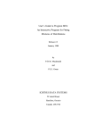
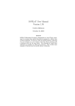
opposite in directions at the two ends of the member. The figure 2.1 below shows
some common type of truss:
Pratt truss
King post truss
Town‟s lattice truss
Figure 2.1: Types of truss
Planar truss or plane truss is a truss where all the members and nodes are
lying within a two-dimensional plane. Space truss is a truss that having members and
nodes extending into three dimensions.
In structural analysis, there are several methods that can be used to analysis
truss which are method of joints, method of sections, finite element method and etc.
The method of joints uses the concept of equilibrium of joints and has
become the basis for all trusses analysis directed towards finding the unknown forces
in the truss structure. A truss is considered to be composed of a series of members
and joints. Member forces are found by considering all the joints are in a state of
equilibrium. For a plane truss, the two independent equations of statics are used
simultaneously to find the member forces ( 𝐹𝑥 = 0 and
will move if there was a net force acting to the joint.
𝐹𝑦 = 0). However, a joint
6
The method of sections is a method in where firstly cut the truss structure into
sections, then replace the removed section with unknown member forces acting in
the direction of the cut member. The forces in the members are then computed by
summing the unknown forces by using equilibrium equations ( 𝐹𝑥 = 0,
and
𝐹𝑥 = 0
𝑀 = 0). Since there are only three equilibrium equations, the truss section cut
should be chosen properly and located at where there are only three unknown
member forces.
2.3
Finite Element Method
The finite element method (FEM) or sometimes referred to as finite element
analysis (FEA) is a general numerical technique for approximating the behaviour if
continua by assembly of small parts (elements). It is much easier to analyze each
element separately than the whole structure due to its simple geometry. In essence a
complicated solution is approximated by a model that consists of piecewisecontinuous simple solutions. (Finite Element Method For Structural Analysis,
Redzuan Abdullah 2010)
The modern development of the finite element method began in the 1940s in
the field of structural engineering with the work by Hrennikoff in 1941 and
MCHenry in 1943, who used a lattice of line (one-dimensional) elements (bars and
beams) for the solution of stresses in continuous solids. Levy developed the
flexibility or force method in 1947. The first treatment of two-dimensional elements
was by Turner et al. in 1956. They derived stiffness matrices for truss elements,
beam elements, and two-dimensional triangular and rectangular elements in plane
stress. They also outlined the procedure commonly known as the direct stiffness
method for obtaining the total structure stiffness matrix. The work of Turner et al.
prompted further development of finite element stiffness equations expressed in
matrix notation in pace with the development of the high-speed digital computer in
the early 1950s. Clough introduced the phrase finite element in 1960. Extension of
the finite element method to three-dimensional problems with the development of a
7
tetrahedral stiffness matrix was done by Martin in 1961, by Gallagher et al. in 1962,
and by Melosh in 1963. From the early 1950s to the present, enormous advances
have been made in the application of the finite element method to solve complicated
engineering problems. (A First Course in the Finite Element Method, Fourth Edition,
Daryl L. Logan 2007)
The general procedures of the finite element method are consisting of three
stages, which are pre-processing, solution and post processing.
1. Pre-processing

Identify the geometric domain of the problem

Discretize the problem into elements

Identify the type of element to be used

Apply the boundary conditions (physical constraints)

Define the loadings
2. Solution

Assemble the stiffness matrix K

Solve the governing algebraic equations KQ = F to obtain the
unknown values of the primary field variables (displacement, Q
and reaction forces, F for stress analysis problem).
3. Post processing

The computed values are then used to compute derived variables
(elements stresses and strains) by back substitution.
8
2.4
MATLAB
2.4.1 History
By referring to Getting Started with MATLAB, The MathWorks, Inc. (2005),
MATLAB was originally written to provide easy access to matrix software
developed by the LINPACK (a software library for performing numerical linear
algebra on digital computers) and EISPACK (a software library for numerical
computation of eigenvalues and eigenvectors of matrices) projects. In 20th century, a
newer set of latest set of libraries were rewrote for matrix manipulation known as
LAPACK (a software library for numerical linear algebra) to supersede LINPACK
and EISPACK. Today, MATLAB engines embed the state of the art in software for
matrix computation by incorporating the LAPACK and BLAS libraries. MATLAB
has evolved over a period of years. It is now the standard instructional tool for
introductory and advanced courses in mathematics, engineering, and science in
university environments. On the other hand, it is the tool of choice for highproductivity research, development, and analysis in industry.
2.4.2 Applications in MATLAB
MATLAB is a high-performance programming language developed by The
MathWorks for technical computing. It is a great tool for simulation and data
analysis. It allows us integrate computation, visualization, and programming in a
convenient way and express the solution in familiar mathematical notation. It
provides an excellent computational language, built-in state-of-the-art algorithms for
mathematics and excellent visualization using ready-made functions. Furthermore,
MATLAB is a modern programming language environment: it has sophisticated data
structures, contains built-in editing and debugging tools, and supports object-oriented
programming. These factors make MATLAB an excellent tool for teaching and
research. The most common uses of MATLAB including:
9
i.
Math and computation
ii.
Matrix manipulation
iii.
Algorithm development
iv.
Data acquisition
v.
Plotting of functions and data
vi.
Modelling, simulation, and prototyping
vii.
Data analysis, exploration, and visualization
viii.
Application development, including graphical user interface building
The use of MATLAB is available for many computer systems including MS
windows, Linux and Macintosh. The MATLAB system consists of five main parts
which are:
i.
The MATLAB Language
ii.
Desktop Tools and Development Environment
iii.
Graphics
iv.
The MATLAB Mathematical Function Library
v.
The MATLAB External Interfaces/API.
The MATLAB Language is a high-level matrix/array language with control
flow statements, functions, data structures, input/output, and object-oriented
programming features. It allows the user to program in the small (creating quickly
throw-away programs) and program in the large (creating large and complicated
application-specific programs).
Desktop Tools and Development Environment is a set of tools and facilities
that help user in using MATLAB functions and files. Many of these tools are
graphical user interfaces (GUIs). Examples of the tools and facilities are the
MATLAB desktop and Command Window, a command history, an editor and
debugger, and browsers for viewing help, the workspace, files, and the search path.
Graphics is the MATLAB graphic system. MATLAB has extensive facilities
for displaying, annotating and printing various graphs. It can be used for twodimensional and three-dimensional data visualization, image processing, animation,
10
and presentation by using high-level functions. It also allows the user to fully
customize the appearance of graphics and build complete graphical user interfaces
(GUIs) on MATLAB application by using low-level functions.
The MATLAB Mathematical Function Library is an enormous collection of
computationally efficient and robust algorithms and functions ranging from
elementary functions (sine, cosine, tangent, cotangent, etc.) to specialized functions
(matrix inverse, matrix eigenvalues, Bessel functions, fast Fourier transforms, etc.)
commonly used in scientific and engineering practice.
The MATLAB External Interfaces/API is a library that allows the user to
write C and FORTRAN programs that interact with MATLAB. It includes facilities
for calling routines from MATLAB (dynamic linking), calling MATLAB for
computing and processing, reading and writing M-files, etc.
2.4.3 Advantages using MATLAB
Nowadays there are many other programming softwares that having the
ability to analysis structure by using finite element method such as Visual Basic, C,
FORTRAN, etc. However, MATLAB is chosen for this study because of some
advantages:
i.
Dimensionless
One of the most important features of MATLAB compared to other
high-performance programming languages is that MATLAB does not
require dimensioning, which allows the user to perform matrix
computations efficiently. This is due to MATLAB is an interactive
system whose basic data element is an array that does not require
dimensioning.
11
ii.
Toolboxes
MATLAB is extensible with toolboxes in various application areas,
which allow the user to learn and apply specialized technology.
Toolboxes are comprehensive collections of MATLAB functions (Mfiles) that extend the MATLAB environment to solve particular
classes of problem. Examples of areas in which toolboxes are
available including control systems, neural networks, simulation, etc.
iii.
Matrix optimized
MATLAB is optimized for matrices. Thus, if a problem can be
formulated with a matrix solution, MATLAB executes substantially
faster than a similar program in a high-level language.
iv.
Credit
MATLAB is well developed and well tested with its long history. It
makes use of highly respected algorithms and hence you can be
confident about your results.
In general, MATLAB is a useful tool for vector and matrix manipulations.
Since the majority of the engineering systems are represented by matrix and vector
equations, we can relieve our workload to a significant extent by using MATLAB.
The finite element method which is used in this research is a well-defined candidate
for which MATLAB can be very useful as a solution tool. Matrix and vector
manipulations are essential parts in the method.
CHAPTER 3
METHODOLOGY
3.1
Assumption used in the Research
There are various types of trusses. It is ideal to develop a software that can be
used for analysis of any type of truss. However, this research is only focus in space
truss analysis. The following are the assumptions and limitations in this research:
i.
The program is limited to the analysis of space truss analysis only.
ii.
The mathematical model for a space truss analysis consists of a set of
joints (nodes) which are connected by straight member in three
dimensional spaces.
iii.
All loads acting on the structure must be consists of concentrated
loads act on the joints of the structure only. Intermediate loads acting
on the members or moments acting on the joints of the structure are
not permitted.
iv.
There is no shear force or bending moment exists in the truss
members. The truss members only subjected to compression forces or
tension forces.
v.
There are only reactions forces exist at the support joints of the
structure.
13
vi.
The self-weight of truss members is small and can be neglected in the
analysis.
vii.
Forces acting on the structure are only permitted for directions in xaxis, y-axis or z-axis.
viii.
3.2
The truss members are assumed having linear elastic behaviour.
ix.
The supports of the structure are assumed lie on the horizontal plane.
x.
The inclined support of the structure is not permitted in the analysis.
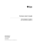
Research Design and Procedure
The research design is shown in figure 3.1 below:
Identify the
problem
Discretize the problem
Determine the member
stiffness matrix
Model the structure
in MATLAB (GUIs)
Establish the structure
stiffness matrix (K)
Apply boundary
conditions
Analyze the
problem
Establish load vector
Solve the equation KQ
=F
Display of results
Post processing stage
Figure 3.1: Research design and procedure
14
a) Identify the model of the space truss structure to be analysed,
including all the coordinates of the joints of the structure.
b) Model the space truss structure in graphical user interfaces (GUIs) of
software MATLAB. Inputs all the important values such as Young‟s
Modulus and area for material properties, type of support for support
condition, and any external forces acting on the structure.
c) Run the analysis after all the inputs needed have been input in the
software MATLAB. The software MATLAB will analysis the
problem through the steps in finite element formulation as following:
i.
Discretize the problem into elements and nodes.
ii.
Determine the stiffness matrix for each element.
iii.
Assemble the element member stiffness matrix to form the
structure stiffness matrix (global stiffness matrix).
iv.
Apply the boundary conditions of the problem.
v.
Define the loadings.
vi.
Solve
the
equation
𝐾 𝑄 = 𝐹
to
obtain
nodal
displacements and consequently reaction forces at the supports.
vii.
Proceed with post processing stage, the computation of
stresses and strains.
d) Display all the important results in software MATLAB.
3.3
Modelling of Truss Structure
In order for the software MATLAB can analysis the truss problem, user has
to model it and input all the needed input in the software first. Graphical user
interfaces (GUIs) in MATLAB is used as the medium for user input values and
model the structure.
15
3.4
Analysis of Truss Structure
Finite element formulation is used as the method for the analysis of truss in
this research. There are several approaches that can be used to define and formulate
the finite element problem. The most widely used method in this research is the
direct stiffness method where it can yield the displacements and forces directly. The
internal force, stress and strain in each element can then be determined by backsubstitution of displacements into individual element equations. The detail of space
truss finite element formulation is presented in the following section.
3.4.1 Discretize the Problem
Figure 3.2: A simple space truss example
16
z
y’
d
z’
2
θz
1
θy
y
θx
x
x’
Figure 3.3: A truss element in three-dimensional space
In general, pin-jointed structures which do not have loading between joints or
moments at joints such as trusses, can be subdivided into elastic spring/bar elements
for analysis. A spring/bar element is a one dimensional element and has linear
interpolation function. Figure 3.2 shows a simple space truss example. Figure 3.3
shows one of the elements of the space truss. The truss is discretized into six finite
elements which are connected to each other at joints referred to as nodes.
Degree of freedom is defined as the possible displacements of the node. For a
three dimensional space truss problem, there are three degrees of freedom for each
node of the structure. These degrees of freedom are the displacements in x-direction,
y-direction and z-direction of the node, as shown in Figure 3.3.
17
3.4.2 Determine the Element Stiffness Matrix
After discretize the truss into bar elements, a shape function is needed to be
assumed to represent the physical behaviour of an element. A shape function is an
approximate continuous function expressed in terms of two nodal variables u 1 and u2.
Figure 3.4 below shows an elastic bar element with length L, which is affixed an
uniaxial coordinate system x with its origin placed at the left hand.
q1
q2
x
1
2
u(x)
x
L
Figure 3.4: A bar element in local direction
The axial displacement at any position along the length of the element is
denoted as u(x). The nodal displacement at x = 0 (node 1) and x = L (node 2) are
denoted as 𝑢 0 = 𝑞1 and 𝑢 𝐿 = 𝑞2 respectively. The axial displacement function
can be expressed in term of x by assuming linear interpolation for displacement:
𝑢(𝑥) = 𝑎0 + 𝑎1 𝑥
(3.1)
From the boundary conditions, 𝑢 0 = 𝑞1 and 𝑢 𝐿 = 𝑞2 , the shape functions
can be determined as follow:
𝑢 0 = 𝑎0 + 𝑎1 0 = 𝑞1
gives 𝑎0 = 𝑞1
𝑢 𝐿 = 𝑎0 + 𝑎1 𝐿 = 𝑞2
⇒ 𝑞1 + 𝑎1 𝐿 = 𝑞2
gives 𝑎1 =
𝑞2 – 𝑞1
𝐿
18
Then
𝑢 𝑥 = 𝑞1 +
𝑞2 – 𝑞1
𝐿
𝑥
𝑥
⇒ 𝑢 𝑥 = 1 − 𝐿 𝑞1 +
𝑞1
= 𝑁1 𝑁2 𝑞
2
𝑥
𝐿
𝑞2
(3.2)
𝑥
𝑥
where 𝑁1 = 1 − 𝐿 , 𝑁2 = 𝐿
= 𝑁 𝑞
(3.3)
By recalling back from the elementary strength of materials, the deflection, δ
of an elastic bar of length, L with uniform cross-sectional area, A when subjected to
an axial load, P is given by:
𝑃𝐿
𝛿 = 𝐴𝐸
(3.4)
where E = Young modulus of elasticity of the material
From equation (3.4), the equivalent spring constant of an elastic bar can be
obtained as:
𝑃
𝑘=𝛿 =
𝐴𝐸
𝐿
(3.5)
When a bar element is subjected to a uniaxial loading, the normal strain
component is defined as:
𝑑𝑢
𝜀 = 𝑑𝑥
(3.6)
Substitute equation (3.2) into equation (3.6) will give
𝑞1
1
𝜀 = 𝐿 −1 1 𝑞
2
(3.7)
19
The strain is constant in an element that has constant cross-sectional area and
subjected to constant forces at the points. By Hooke‟s law, the axial stress in the bar
element is defined as:
𝐸
𝜎 = 𝐸𝜀 =
𝐿
𝑞1
−1 1 𝑞
2
(3.8)
This axial stress is then related to the axial force gives:
𝑃 = 𝜎𝐴 =
𝐴𝐸
𝐿
𝑞1
−1 1 𝑞
2
(3.9)
Equation (3.9) can be used to relate nodal forces with the nodal displacements.
Be noted that equation (3.9) has a positive value when the element is subjected to
tension force and has a negative value when the element is subjected to compression
force. Nodal forces of an element at node 1 (f1) and node 2 (f2) must be of same
magnitude but opposite direction for equilibrium. Hence,
𝑞1
−1
1
𝑞2
𝐿
𝑞1
𝐴𝐸
𝑓2 = 𝐿 −1 1 𝑞
2
𝑓1 = −
𝐴𝐸
(3.10)
(3.11)
Equation (3.10) and (3.11) can be combined to yield
𝐴𝐸
𝐿
𝑓
−1 𝑞1
= 1
𝑞
𝑓2
1
2
1
−1
(3.12)
or
𝑘 𝑞 = 𝑓
(3.13)
where the element stiffness matrix for the bar element is given as:
𝑘 =
𝐴𝐸
𝐿
1 −1
−1 1
(3.14)
20
Equation (3.14) shows that the element stiffness matrix for a bar element is
symmetric and in order of 2 × 2 corresponding to two degrees of freedom or two
nodal displacements in a bar element. This equation only gives the element stiffness
matrix in the element coordinate system, which is in one dimensional. In order to
analyze a three dimensional space truss, the element stiffness matrix for each
member of the truss must be transformed and expressed in global coordinate system
first.
For a space truss, each node of the member has three degrees of freedom or
nodal displacements in global coordinates. The relationship between the element
displacements in the element coordinate system and the global coordinate system can
be defined as:
𝑞1 = 𝑄1𝑥 𝜆𝑥 + 𝑄1𝑦 𝜆𝑦 + 𝑄1𝑧 𝜆𝑧
(3.15)
𝑞2 = 𝑄2𝑥 𝜆𝑥 + 𝑄2𝑦 𝜆𝑦 + 𝑄2𝑧 𝜆𝑧
(3.16)
where 𝑄1𝑥 , 𝑄1𝑦 , 𝑄1𝑧 = displacements at node 1 in global x-axis, y-axis and z-axis
directions respectively,
𝑄2𝑥 , 𝑄2𝑦 , 𝑄2𝑧 = displacements at node 2 in global x-axis, y-axis and z-axis
directions respectively,
𝜆𝑥 = 𝑐𝑜𝑠 𝜃𝑥 , 𝜆𝑦 = 𝑐𝑜𝑠 𝜃𝑦 , 𝜆𝑧 = 𝑐𝑜𝑠 𝜃𝑧
Equation (3.15) and (3.16) can be written in matrix form as:
𝑞1
𝜆𝑥
=
𝑞2
0
𝜆𝑦
0
𝜆𝑧
0
0
𝜆𝑥
0
𝜆𝑦
0
𝜆𝑧
𝑄1𝑥
𝑄1𝑦
𝑞 = 𝑇 𝑄
𝑄1𝑧
𝑄2𝑥
𝑄2𝑦
𝑄2𝑧
(3.17)
where
𝑇 =
𝜆𝑥
0
𝜆𝑦
0
𝜆𝑧
0
0
𝜆𝑥
0
𝜆𝑦
0
𝜆𝑧
(3.18)
𝑇
21
[𝑇] is referred to as the displacement transformation matrix because it
transform the global displacements into the element local displacement.
The relationship between the global force components and the local forces
can be defined as:
𝐹1𝑥 = 𝑓1 𝜆𝑥
𝐹1𝑦 = 𝑓1 𝜆𝑦
𝐹1𝑧 = 𝑓1 𝜆𝑧
𝐹2𝑥 = 𝑓2 𝜆𝑥
𝐹2𝑦 = 𝑓2 𝜆𝑦
𝐹2𝑧 = 𝑓2 𝜆𝑧
which can be written in matrix form as:
𝐹1𝑥
𝐹1𝑦
𝐹1𝑧 𝐹2𝑥
𝐹2𝑦
𝐹2𝑧
𝑇
𝜆𝑥
0
=
𝐹 = 𝑇
𝑇
𝜆𝑦
0
0
𝜆𝑥
𝜆𝑧
0
0
𝜆𝑦
0
𝜆𝑧
𝑓
𝑓1
𝑓2
(3.19)
where
𝑇
𝑇
𝜆𝑥
0
=
𝜆𝑦
0
𝜆𝑧
0
0
𝜆𝑥
0
𝜆𝑦
0
𝜆𝑧
𝑇
(3.20)
The results are combined together to determine the stiffness matrix for a
member which relates the member‟s global force components {𝐹} to its global
displacement {𝑄}. Substitute equation (3.17) and (3.19) into (3.13) yields
𝑘 𝑞 = 𝑓
𝑇
𝑇
𝑘 𝑇 𝑄 = 𝑓
(3.21)
𝑘 𝑇 𝑄 = 𝐹
(3.22)
𝐾′ 𝑄 = 𝐹
(3.23)
where
𝐾′ =
𝜆𝑥
0
𝜆𝑦
0
𝜆𝑧
0
0
𝜆𝑥
0
𝜆𝑦
0
𝜆𝑧
𝑇
𝐴𝐸
𝐿
1 −1 𝜆𝑥
−1 1
0
𝜆𝑦
0
𝜆𝑧
0
0
𝜆𝑥
0
𝜆𝑦
0
𝜆𝑧
22
(3.24)
The member stiffness matrix expressed in global coordinates for each
member of the space truss can be determined by using equation (3.24) above.
3.4.3 Assemble the Global Stiffness Matrix
Once the member stiffness matrix for each of the member of the truss is
determined, the structure stiffness matrix can then be determined by assembling all
the member stiffness matrices to represent the entire truss.
The rows and columns of the member stiffness matrix are designated by the
code numbers which are used to identify the global degrees of freedom that occur at
each end of the member. The structure stiffness matrix will have an order that equal
to the highest code number assigned to the truss. For example, a tetrahedron will
have structure stiffness matrix with order 12 × 12 corresponding to total of twelve
degrees of freedom where three degrees of freedom for each of the four nodes. When
the member stiffness matrices are assembled, each element in the matrix will then
placed in its same row and column designation in the structure stiffness matrix.
23
3.4.4 Apply the Boundary Conditions
Once the structure stiffness matrix is obtained, the boundary conditions will
be applied where there are supports or external forces at the nodes. The external
forces at the nodes can be directly assigned to the elements in the external force
matrix with corresponding degrees of freedom and rows code numbers. On the other
hand, the supports at the nodes will restrain the nodes from moving and therefore do
not have displacement. Direction of movement restraint is governed by the type and
orientation of the support. These displacements which are zero value are assigned to
the elements in the displacement matrix with corresponding degrees of freedom and
rows code numbers. An equation relating unknown displacements to known external
forces can then be formed.
𝐾𝑟𝑒𝑑𝑢𝑐𝑒
𝑄𝑢 = 𝐹𝑘
(3.25)
where [𝐾𝑟𝑒𝑑𝑢𝑐𝑒] = reduced structure stiffness matrix
{𝑄𝑢} = unknown displacements matrix
{𝐹𝑘} = known external forces matrix
3.4.5 Solve the Equations
The values of unknown displacements can be determined by solving the
equation (3.25). Subsequently, the components of reaction forces can be determined
by substituting the values of the unknown displacements obtained above into the
structure stiffness equation as shown below:
𝐾 𝑄 = 𝐹
where [𝐾] = structure stiffness matrix
{𝑄} = global displacements matrix
{𝐹} = global force components matrix
(3.26)
24
3.4.6 Post Processing Stage
The final computational step in finite element analysis of a truss is to
determine the internal force, strain and stress in each element of the truss by making
use of the global displacements obtained in the steps previously. The internal force or
member force can be determined using equation (3.21):
𝑘 𝑇 𝑄 = 𝑓
𝑓1
=
𝑓2
𝐴𝐸
𝐿
1
−1
−1 𝜆𝑥
1
0
𝜆𝑦
0
0
𝜆𝑥
𝜆𝑧
0
0
𝜆𝑦
0
𝜆𝑧
𝑄1𝑥
𝑄1𝑦
𝑄1𝑧 𝑄2𝑥
𝑄2𝑦
𝑄2𝑧
𝑇
(3.27)
The strain in the element of the truss can be determined by substituting
equation (3.17) into (3.7):
1
𝜀 = 𝐿 −1 1 𝑞
1
= 𝐿 −1 1 𝑇 𝑄
1
= 𝐿 −1 1
𝑄1𝑥
𝜆𝑥
0
𝑄1𝑦
𝜆𝑦
0
𝑄1𝑧
𝜆𝑧
0
𝑄2𝑥
0
𝜆𝑥
𝑄2𝑦
0
𝜆𝑦
0
𝜆𝑧
𝑄2𝑧
𝑇
(3.28)
The stress in the element of the truss can be determined by substituting
equation (3.28) into (3.8):
𝜎 = 𝐸𝜀
=
𝐸
𝐿
−1 1
𝑄1𝑥
𝜆𝑥
0
𝑄1𝑦
𝜆𝑦
0
𝜆𝑧
0
𝑄1𝑧 𝑄2𝑥
0
𝜆𝑥
𝑄2𝑦
0
𝜆𝑦
𝑄2𝑧
0
𝜆𝑧
𝑇
(3.29)
25
3.5
MATLAB Graphical User Interface Development Environment (GUIDE)
The graphical user interface development environment (GUIDE) function in
MATLAB provides a set of tools for creating graphical user interfaces (GUIs). These
tools simplify the process of laying out and programming GUIs. When a GUI is
opened in GUIDE, it is displayed in the Layout Editor, which is the control panel for
all of the GUIDE tools. The following figure shows the Layout Editor with a blank
GUI template.
Component Palette
Figure (Layout area)
Figure 3.5: Layout Editor with a blank GUI in GUIDE
You can lay out your GUI by dragging components, such as panels, push
buttons, pop-up menus, or axes, from the component palette, at the left side of the
Layout Editor, into the layout area. Some of the important components used in
developing the graphical user interfaces in this research will be discussed in this
section.
26
3.5.1 Figure
Figure objects are the individual windows on the screen in which the
MATLAB software displays graphical output. In this research, the figure is as shown
in Figure 3.6.
3.5.2 Static Text
Static text boxes display lines of text. Static text is typically used to label
other controls, provide directions to the user, or indicate values associated with a
slider. Users cannot change static text interactively. Static text controls do not
activate callback routines when clicked. Example of static text in GUI of the space
truss analysis program is shown in Figure 3.6.
3.5.3 Edit Text
Editable text fields enable users to enter or modify text values. Editable text
is often used when text is wanted as input. If Max-Min>1, then multiple lines are
allowed. For multi-line edit boxes, a vertical scrollbar enables scrolling, as do the
arrow keys. To obtain the string a user types in an edit box, get the string property.
Examples of code used in this research to obtain text or string from edit boxes are as
following.
% Obtain data from edit1, edit2, edit3, edit4, edit5 and edit6.
xLimit(1) = str2double(get(handles.edit1,'string'));
yLimit(1) = str2double(get(handles.edit2,'string'));
zLimit(1) = str2double(get(handles.edit3,'string'));
xLimit(2) = str2double(get(handles.edit4,'string'));
yLimit(2) = str2double(get(handles.edit5,'string'));
zLimit(2) = str2double(get(handles.edit6,'string'));
27
Figure
Static Text
Edit Text
Figure 3.6: Figure, static text and edit text in GUI
3.5.4 Table
Tables contain rows of numbers, text strings, and choices grouped by
columns. Rows and columns can be named or numbered. Entire tables or selected
columns can be made user-editable. Data in each column must of the same type of
data. The number of rows and columns automatically adjust to reflect the size of the
data matrix the table displays. Tables are useful in presenting data which is in array
structure or matrix. The property values of a table can be set and query using the set
and get functions. Examples of code used in this research to obtain data from tables
and set the data in tables are as following.
% Obtain data from table_node and table_element.
data_node = get(handles.table_node,'data');
data_element = get(handles.table_element,'data');
% Set the data in table_node and table_element.
set(handles.table_node,'data',data_node)
set(handles.table_element,'data',data_element)
28
3.5.5 Push Button
The push button is perhaps the most prevalent MATLAB user interface
control (uicontrol) style. It is used primarily to indicate that a desired action should
immediately take place. When the user clicks on a push button, it invokes an event
immediately. The event is dictated by the code that is programmed in the push
button‟s callback function. The „Cancel‟ button in Figure 3.7 when clicked by the
user will close the table and go back to the screen before. Example of code for the
“Cancel” button is shown below.
% --- Executes on button press in pushbutton8.
function pushbutton8_Callback(hObject, eventdata, handles)
% hObject
handle to pushbutton8 (see GCBO)
% eventdata reserved - to be defined in a future version of MATLAB
% handles
structure with handles and user data (see GUIDATA)
set(handles.table_insert,'visible','off')
set(handles.pushbutton7,'visible','off')
set(handles.pushbutton8,'visible','off')
Table
Figure 3.7: Table and push button in GUI
Push Button
29
3.5.6 Axes
Axes components enable your GUI to display graphics, such as graphs and
images. While the basic purpose of an axes object is to provide a coordinate system
for plotted data, axes properties provide considerable control over the way MATLAB
displays data. The current axes is the target for functions that draw image, line, patch,
rectangle, surface, and text graphics objects. Axis manipulates commonly used axes
properties. Code axis([xmin xmax ymin ymax zmin zmax]) sets the x-, y-, and z-axis
limits of the current axes. The axes component in this research is shown in Figure 3.9.
Examples of code used in this research to set the axis limits of axes and plot the
space truss structure in axes are as following.
% Set the x-, y-, and z-axis limits of the axes.
axis([xLimit(1) xLimit(2) yLimit(1) yLimit(2) zLimit(1) zLimit(2)])
% Plot the space truss structure in the axes.
for i=1:t
% Plot the nodes of the space truss structure
plot3(node_xyz{i,1},node_xyz{i,2},node_xyz{i,3},...
'Marker', 'o','MarkerFaceColor','b')
text(node_xyz{i,1}+(xmax-xmin)/50,node_xyz{i,2}+...
(ymax-ymin)/50,node_xyz{i,3}+(zmax-zmin)/50, ...
num2str(i),'Color','r','FontWeight','bold')
hold on
end
for i=1:n/2
% Plot the elements of the space truss structure
plot3([node_xyz{dof(2*i-1),1} node_xyz{dof(2*i),1}],...
[node_xyz{dof(2*i-1),2} node_xyz{dof(2*i),2}],...
[node_xyz{dof(2*i-1),3} node_xyz{dof(2*i),3}],'-')
hold on
text(((node_xyz{dof(2*i-1),1}+node_xyz{dof(2*i),1})/2)+...
(xmax-xmin)/40,...
((node_xyz{dof(2*i-1),2}+node_xyz{dof(2*i),2})/2)+ ...
(ymax-ymin)/40,...
((node_xyz{dof(2*i-1),3}+node_xyz{dof(2*i),3})/2)+ ...
(zmax-zmin)/40,...
num2str(i),'EdgeColor','k')
hold on
end
30
3.5.7 Panel
Panels group GUI components and can make a GUI easier to understand by
visually grouping related controls. It can contain user interface controls with which
the user interacts directly. A panel can contain panels and button groups as well as
axes and user interface controls such as push buttons, sliders, pop-up menus, etc. The
position of each component within a panel is interpreted relative to the lower-left
corner of the panel. If you move the panel, the components within the panel
automatically move with it and maintain their positions relative to the panel. Figure
3.8 below shows the list of a panel named “Results (Node and Element)” and its
child objects in object browser. The panel in GUI of the space truss analysis program
is shown in Figure 3.9.
Figure 3.8: List of a panel and its child objects in object browser
31
Axes
Panel
Figure 3.9: Axes and panel in GUI
CHAPTER 4
RESULTS AND ANALYSIS
4.1
Introduction
In this chapter, an example of space truss problem is used to demonstrate the
steps to model and analysis a space truss structure in the space truss analysis program
developed. The results obtained from the space truss analysis program are then
compared with the results obtained from STAAD.Pro in which analysis the same
space truss problem.
In order to validate the space truss analysis program and verify its results, the
results from space truss analysis program developed is compared with results from
existing engineering software, STAAD.Pro. Three examples of space truss problems
are modelled and analysed using both the space truss analysis program developed
and STAAD.Pro in this chapter. The results obtained from the program and the
software should be the same or approximately same.
33
4.2
Space Truss Modelling (User Manual)
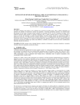
A simple example of space truss problem is taken from MATLAB Guide to
Finite Elements, Peter I. Kattan (2006) as following:
Example 1:
z
12 kN
1
5m
y
x
4
2
2
4m
3
4m
3m
Figure 4.1: Space truss for Example 1
Data available:
Young‟s modulus, E = 200 GPa = 200e+06 kN/m2
Cross-sectional area, A12 = 0.001 m2, A13 = 0.002 m2, A14 = 0.001 m2
Determine:
i.
The x-direction, y-direction and z-direction displacements at nodes.
ii.
The reactions at nodes 2, 3 and 4.
iii.
The force in each element.
iv.
The stress in each element.
34
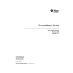
First of all, the range of the axes is determined from the space truss structure
diagram in order to display the space truss structure within the axes range. In the case
of this Example 1, the range of x-axis is from -4 m till 4m, the range of y-axis is from
-3 m till 0 m, and the range of z-axis is from 0 m till 5 m. Example of inputs for this
Example 1 is shown as Figure 4.2 below.
Figure 4.2: Input the range of axes
After input the axes range, press on the „Next‟ button. The axes will then be
generated and displayed on the next interface. To model the space truss structure,
press on the „Insert‟ button on the bottom left of the interface. A table will pop out at
the centre of the interface for inputting coordinates of the start node and end node for
each element of the space truss structure. For this Example 1, the x-coordinate, ycoordinate, z-coordinate of start node and end node for element 1 are 0, 0, 5 and 0, -4,
0. The x-coordinate, y-coordinate, z-coordinate of start node and end node for
element 2 are 0, 0, 5 and -3, 0, 0. Lastly, the x-coordinate, y-coordinate, z-coordinate
of start node and end node for element 3 are 0, 0, 5 and 0, 4, 0. Example of the inputs
is shown in Figure 4.3 below.
35
Figure 4.3: Input the coordinates of nodes of the elements
Once finish input all the members of the space truss structure, press on the
„OK‟ button below the table. Subsequently, the space truss structure will be
generated and displayed on the axes generated before. The number of the nodes and
elements will be displayed on the axes as well. The coordinates of the nodes are also
displayed in the left hand side table with heading „Data (Node and Element)‟. The
appearance of the interface will become as shown in Figure 4.4 below.
36
Figure 4.4: Model of the space truss structure
Now we proceeding to the next stage, that is input all the required data for the
nodes and elements. The support condition of each node is identified and can be
selected from the choices available there, that is ball-and socket (constrained from
translation), roller (constrained from movement in the z-direction) or no support at
all. For this Example 1, the support condition of node 1 is none and the support
condition of node 2, 3 and 4 are all ball-and socket. If the node is supported by roller
or no support at all, the external forces acting at the nodes along x-direction, ydirection and z-direction are identified and input into the node data table. Therefore,
the external forces at node 1 are Fx, Fy and Fz which are equal to 12 kN, 0 kN and 0
kN respectively. Other than that, the Young‟s Modulus and area of each element are
identified and input into the element data table. For this Example 1, the Young‟s
Modulus value is the same for the three elements, which is 200e +06 kN/m2. On the
other hand, the area of element 1 and 3 are both 0.001 m2 while the area of element 2
is 0.002 m2. The figure 4.5 below shows the appearance of the interface after input
all the important data.
37
Figure 4.5: Input the required data for analysis
The space truss analysis program is now ready to analysis the space truss
problem as in Example 1. Press on the „Analyse‟ button below the element data table,
the space truss problem will be analysed based on finite element method and the
results will be displayed in the node result table and element result table as shown in
Figure 4.6 below.
38
Figure 4.6: Analysis and display of the results
4.3
Comparison of Results
The same space truss problem as in Example 1 is modelled and analysed
using engineering software STAAD.Pro. The results obtained are compared with the
results obtained previously by using space truss analysis program developed. The
comparisons of the two results are shown in Table 4.1, Table 4.2, Table 4.3 and
Table 4.4 below.
39
Table 4.1: Displacements at nodes (Example 1)
Node Displacements
Number
of node
Space Truss Analysis Program (m)
STAAD.Pro (m)
Ux
Uy
Uz
Ux
Uy
Uz
1
0.0015
1.3616e-19
-5.2506e-04
1.536e-3
0.000
-0.525e-3
2
0
0
0
0.000
0.000
0.000
3
0
0
0
0.000
0.000
0.000
4
0
0
0
0.000
0.000
0.000
Table 4.1 above shows the comparison of the nodes displacements obtained
from the two analysis program and software. We can see that the results from both
the program and the software are almost the same. The displacement at node 1 in ydirection, Uy is 1.3616e-19 m in space truss analysis program, but it is 0 m in
engineering software STAAD.Pro. This may be due to the value is too small that
STAAD.Pro treat it as zero.
Table 4.2: Reactions at supports (Example 1)
Reactions
Number
of node
Space Truss Analysis Program (kN)
STAAD.Pro (kN)
Rx
Ry
Rz
Rx
Ry
Rz
2
-7.8416e-16
8.0000
10.0000
0.000
8.000
10.000
3
-12.0000
1.4282e-15
-20.0000
-12.000
0.000
-20.000
4
-7.8416e-16
-8.0000
10.0000
0.000
-8.000
10.000
40
Comparison of reactions as obtained from space truss analysis program and
STAAD.Pro is shown in Table 4.2 above. Most of the results obtained from space
truss analysis program are same as the results obtained from STAAD.Pro, except that
some reactions which are very small value in space truss analysis program are shown
as zero in STAAD.Pro.
Table 4.3: Force in elements (Example 1)
Force In Element
Number of
Element
Space Truss Analysis Program
(kN)
STAAD.Pro (kN)
1
-12.8062
-12.806
2
23.3238
23.324
3
-12.8062
-12.806
From Table 4.3, we can see the comparison of forces in the elements of the
space truss structure. The results of forces in elements are the same when analyse the
Example 1 by using space truss analysis program and STAAD.Pro.
Table 4.4: Stress in elements (Example 1)
Stress In Element
Number of
Element
Space Truss Analysis Program
2
(kN/m )
STAAD.Pro (kN/m2)
1
-1.2806e+04 (Compressive)
-12.806e+03 (Compressive)
2
1.1662e+04 (Tensile)
11.662+03 (Tensile)
3
-1.2806e+04 (Compressive)
-12.806+03 (Compressive)
41
Table 4.4 above shows the comparison of the elements internal stresses
obtained from the two analysis program and software. The comparison shows that
the analysis results from the space truss analysis program are identical with the
results from the engineering software STAAD.Pro. The positive value of stress
means the stress is tensile stress while negative value means the stress is compressive
stress.
In order to check the functionality and performance of the space truss
analysis program, two more examples of space truss problems are modelled and
analysed by using the space truss analysis program and then the answers are
compared with those obtained from engineering software STAAD.Pro.
Example 2:
z
15 kN
1
20 kN
x
5m
5
y
4
2
4m
2
3m
3
3m
3m
Figure 4.7: Space truss for Example 2
Data available:
Young‟s modulus, E = 200 GPa = 200e+06 kN/m2
Cross-sectional area, A = 0.003 m2
42
Determine:
i.
The x-direction, y-direction and z-direction displacements at nodes.
ii.
The reactions at nodes 2, 3, 4 and 5.
iii.
The force in each element.
iv.
The stress in each element.
Figure 4.8 below shows the appearance of the interface of space truss analysis
program after the space truss problem as in Example 2 is modelled and analysed
using the program.
Figure 4.8: Analysis and display of the results for Example 2
The results obtained from the space truss analysis program are compared with
those from STAAD.Pro as shown in Table 4.5, Table 4.6, Table 4.7 and Table 4.8
below.
43
Table 4.5: Displacements at nodes (Example 2)
Node Displacements
Number
of node
Space Truss Analysis Program (m)
STAAD.Pro (m)
Ux
Uy
Uz
Ux
Uy
Uz
1
2.3509e-04
-3.6713e-04
2.5875e-07
0.235e-3
-0.367e-3
0.000
2
0
0
0
0.000
0.000
0.000
3
0
0
0
0.000
0.000
0.000
4
0
0
0
0.000
0.000
0.000
5
0
0
0
0.000
0.000
0.000
Table 4.6: Reactions at supports (Example 2)
Reactions
Number
of node
Space Truss Analysis Program (kN)
STAAD.Pro (kN)
Rx
Ry
Rz
Rx
Ry
Rz
2
-1.1887e-15
9.9883
16.6471
0.000
9.988
16.647
3
-6.4151
7.6349e-16
-10.6919
-6.415
0.000
-10.692
4
1.1915e-15
10.0117
-16.6862
0.000
10.012
-16.686
5
-8.5849
-8.4148e-16
10.7311
-8.585
0.000
10.731
44
Table 4.7: Force in elements (Example 2)
Force In Element
Number of
Element
Space Truss Analysis Program
(kN)
STAAD.Pro (kN)
1
-19.4137
-19.414
2
12.4688
12.469
3
19.4593
19.459
4
-13.7425
-13.742
Table 4.8: Stress in elements (Example 2)
Stress In Element
Number of
Element
Space Truss Analysis Program
2
(kN/m )
STAAD.Pro (kN/m2)
1
-6.4712e+03 (Compressive)
-6.471e+03 (Compressive)
2
4.1563e+03 (Tensile)
4.156+03 (Tensile)
3
6.4864e+03 (Tensile)
6.486+03 (Tensile)
4
-4.5808e+03 (Compressive)
-4.581e+03 (Compressive)
From the comparison as shown in Table 4.5, Table 4.6, Table 4.7 and Table
4.8 above, we can see that the results obtained from the space truss analysis program
and STAAD.Pro are approximately the same except that the results values obtained
from STAAD.Pro show less decimal places than the results values obtained from
space truss analysis program developed.
45
Example 3:
z
4
3m
6m
x
1
15 kN
y
3
6m
3m
4m
2
Figure 4.9: Space truss for Example 3
Data available:
Young‟s modulus, E = 200 GPa = 200e+06 kN/m2
Cross-sectional area, A12 = 0.001 m2, A13 = 0.002 m2, A14 = 0.005 m2
Determine:
i.
The x-direction, y-direction and z-direction displacements at nodes.
ii.
The reactions at nodes 1, 2, 3 and 4.
iii.
The force in each element.
iv.
The stress in each element.
46
The appearance of the interface of space truss analysis program after the
space truss problem as in Example 3 is modelled and analysed using the program is
shown in Figure 4.10 below.
Figure 4.10: Analysis and display of the results for Example 3
Similarly, the results obtained from the space truss analysis program are
compared with those from STAAD.Pro as shown in Table 4.9, Table 4.10, Table
4.11 and Table 4.12 below.
47
Table 4.9: Displacements at nodes (Example 3)
Node Displacements
Number
of node
Space Truss Analysis Program (m)
STAAD.Pro (m)
Ux
Uy
Uz
Ux
Uy
Uz
1
-0.0016
-0.0037
0
-1.562e-3
-3.743e-3
0.000
2
0
0
0
0.000
0.000
0.000
3
0
0
0
0.000
0.000
0.000
4
0
0
0
0.000
0.000
0.000
Table 4.10: Reactions at suppots (Example 3)
Reactions
Number
of node
Space Truss Analysis Program (kN)
STAAD.Pro (kN)
Rx
Ry
Rz
Rx
Ry
Rz
1
0
0
-35.2596
0.000
0.000
-35.260
2
30.0000
-2.2078e-15
20.0000
30.000
0.000
20.000
3
-14.7404
7.3702
1.0091e-15
-14.740
7.370
0.000
4
-15.2596
7.6298
15.2596
-15.260
7.630
15.260
48
Table 4.11: Force in elements (Example 3)
Force In Element
Number of
Element
Space Truss Analysis Program
(kN)
STAAD.Pro (kN)
1
-36.0555
-36.056
2
16.4803
16.480
3
22.8893
22.889
Table 4.12: Stress in elements (Example 3)
Stress In Element
Number of
Element
Space Truss Analysis Program
2
(kN/m )
STAAD.Pro (kN/m2)
1
-3.6056e+04 (Compressive)
-36.056e+03 (Compressive)
2
8.2402e+03 (Tensile)
8.240+03 (Tensile)
3
4.5779e+03 (Tensile)
4.578+03 (Tensile)
From the comparison as shown in Table 4.9, Table 4.10, Table 4.11 and
Table 4.12 above, we can see that the results obtained from the space truss analysis
program and STAAD.Pro are again approximately the same.
The analysis of the three examples of space truss problems by using space
truss analysis program and STAAD.Pro give the results with approximately same
values. Consequently, this validates the space truss analysis program developed and
verifies its results.
CHAPTER 5
CONCLUSIONS AND RECOMMENDATIONS
5.1
Conclusions
Through the research carried out, the space truss analysis program has been
developed using MATLAB. Space truss problems are analysed and solved by using
finite element formulation programmed in MATLAB.
The efficiency of the program developed and the accuracy of the results
obtained have been validated and verified by comparing the results with those
generated by existing commercial software, which is STAAD.Pro in this research.
The comparison of the two results shows that the results obtained from the program
developed are accurate and acceptable. The displacements at the nodes, the reactions
at the nodes which have support, the internal force and stress inside the elements can
be determined effectively by using the space truss analysis program.
The research has been carried out successfully. The objective of the research
is achieved, that is developing a valid space truss analysis program by applying finite
element method using MATLAB R2009b.
50
5.2
Recommendations
Although in this research the space truss analysis program has been
successfully developed by using MATLAB, the program can be upgraded and
improved in various aspects especially regarding the assumptions and limitations
stated in this research. As mention earlier in the Chapter 3, the space truss analysis
program is limited to the analysis of space truss structure subjected to external forces
which acting in directions along x-axis, y-axis or z-axis only. In the future research,
the space truss analysis program can be improved by making it able to analysis space
truss structure subjected to external forces acting in any directions.
Besides that, the space truss analysis program is also not able to analysis
space truss structure with incline support. There are only two types of horizontal
support conditions available in this space truss analysis program, which are ball-and
socket (constrained from movement in the x-direction, y-direction and z-direction)
and roller (constrained from movement in the z-direction). In order to improve the
usability and flexibility of the program, the incline support can be included in the
program in the future to make the program more applicable to various types of space
truss problems.
51
REFERENCES
1. Airil Yasreen Mohd Yassin and Ahmad Kueh Beng Hong (2008).
Differential, Variational and Finite Element Formulations for
Structural Beams.
2. Daryl L. Logan (2007). A First Course in the Finite Element Method,
6th edition. India: Rahul Print O Pack, Delhi-20.
3. Getting Started with MATLAB, Version 7. The MathWorks, Inc.
4. J. N. Reddy (1993). An Introduction to the Finite Element Method,
2nd edition. McGraw-Hill, Inc.
5. Patrick Marchand and O. Thomas Holland (2003). Graphics and
GUIs with MATLAB, 3rd edition. Chapman & Hall/CRC.
6. Peter I.Kattan. (2006). MATLAB Guide to Finite Elements. An
Interactive Approach. 2nd edition. New York: Springer-Verlag Berlin
Heidelberg.
7. R. C. Hibbeler (2005). Mechanics of Materials, 6th edition. PrenticeHall, Inc.
52
APPENDIX A: MATLAB R2009a script (Space truss modelling)
function varargout = SpaceTruss(varargin)
gui_Singleton = 1;
gui_State = struct('gui_Name',
mfilename, ...
'gui_Singleton', gui_Singleton, ...
'gui_OpeningFcn', @SpaceTruss_OpeningFcn, ...
'gui_OutputFcn', @SpaceTruss_OutputFcn, ...
'gui_LayoutFcn', [] , ...
'gui_Callback',
[]);
if nargin && ischar(varargin{1})
gui_State.gui_Callback = str2func(varargin{1});
end
if nargout
[varargout{1:nargout}] = gui_mainfcn(gui_State, varargin{:});
else
gui_mainfcn(gui_State, varargin{:});
end
% End initialization code - DO NOT EDIT
% --- Executes just before SpaceTruss is made visible.
function SpaceTruss_OpeningFcn(hObject, eventdata, handles,
varargin)
% This function has no output args, see OutputFcn.
% hObject
handle to figure
% eventdata reserved - to be defined in a future version of MATLAB
% handles
structure with handles and user data (see GUIDATA)
% varargin
command line arguments to SpaceTruss (see VARARGIN)
% Choose default command line output for SpaceTruss
handles.output = hObject;
% Update handles structure
guidata(hObject, handles);
grid on
% UIWAIT makes SpaceTruss wait for user response (see UIRESUME)
% uiwait(handles.figure1);
% --- Outputs from this function are returned to the command line.
function varargout = SpaceTruss_OutputFcn(hObject, eventdata,
handles)
% varargout cell array for returning output args (see VARARGOUT);
% hObject
handle to figure
% eventdata reserved - to be defined in a future version of MATLAB
% handles
structure with handles and user data (see GUIDATA)
% Get default command line output from handles structure
varargout{1} = handles.output;
% --- Executes on button press in pushbutton1.
function pushbutton1_Callback(hObject, eventdata, handles)
% hObject
handle to pushbutton1 (see GCBO)
53
% eventdata
% handles
reserved - to be defined in a future version of MATLAB
structure with handles and user data (see GUIDATA)
set(handles.edit1,'visible','off')
set(handles.edit2,'visible','off')
set(handles.edit3,'visible','off')
set(handles.edit4,'visible','off')
set(handles.edit5,'visible','off')
set(handles.edit6,'visible','off')
set(handles.text1,'visible','off')
set(handles.text2,'visible','off')
set(handles.text3,'visible','off')
set(handles.text4,'visible','off')
set(handles.text5,'visible','off')
set(handles.text6,'visible','off')
set(handles.text10,'visible','off')
set(handles.panel1,'visible','off')
set(handles.pushbutton1,'visible','off')
set(handles.pushbutton4,'visible','on')
set(handles.pushbutton5,'visible','on')
set(handles.pushbutton6,'visible','on')
set(handles.table_element,'visible','on')
set(handles.table_node,'visible','on')
set(handles.table_element2,'visible','on')
set(handles.table_node2,'visible','on')
set(handles.panel2,'visible','on')
set(handles.panel3,'visible','on')
set(handles.panel4,'visible','on')
clc
set(handles.axes1,'visible','on');
axes(handles.axes1);
cla reset
global xLimit yLimit zLimit xInterval yInterval zInterval
xLimit(1) = str2double(get(handles.edit1,'string'));
yLimit(1) = str2double(get(handles.edit2,'string'));
zLimit(1) = str2double(get(handles.edit3,'string'));
xLimit(2) = str2double(get(handles.edit4,'string'));
yLimit(2) = str2double(get(handles.edit5,'string'));
zLimit(2) = str2double(get(handles.edit6,'string'));
axis([xLimit(1) xLimit(2) yLimit(1) yLimit(2) zLimit(1) zLimit(2)])
xlabel('x'),ylabel('y'),zlabel('z'),...
grid on
hold on
% --- Executes on button press in pushbutton2.
function pushbutton2_Callback(hObject, eventdata,
% hObject
handle to pushbutton2 (see GCBO)
% eventdata reserved - to be defined in a future
% handles
structure with handles and user data
question_ans = questdlg('Are you sure you want to
'EXIT','Yes','No','No');
if strcmp(question_ans,'Yes')
close(SpaceTruss)
end
handles)
version of MATLAB
(see GUIDATA)
exit?',...
54
% --- Executes on button press in pushbutton4.
function pushbutton4_Callback(hObject, eventdata, handles)
% hObject
handle to pushbutton4 (see GCBO)
% eventdata reserved - to be defined in a future version of MATLAB
% handles
structure with handles and user data (see GUIDATA)
set(handles.table_insert,'visible','on')
set(handles.pushbutton7,'visible','on')
set(handles.pushbutton8,'visible','on')
% --- Executes on button press in pushbutton5.
function pushbutton5_Callback(hObject, eventdata, handles)
% hObject
handle to pushbutton5 (see GCBO)
% eventdata reserved - to be defined in a future version of MATLAB
% handles
structure with handles and user data (see GUIDATA)
cla
set(handles.table_node,'data',[]);
set(handles.table_element,'data',[]);
% --- Executes on button press in pushbutton6.
function pushbutton6_Callback(hObject, eventdata, handles)
% hObject
handle to pushbutton6 (see GCBO)
% eventdata reserved - to be defined in a future version of MATLAB
% handles
structure with handles and user data (see GUIDATA)
data_node = get(handles.table_node,'data');
data_element = get(handles.table_element,'data');
support = data_node(:,4);
tic;
global node n t dof U
for i = 1:t;
a = strcmp(support(i),'None');
b = strcmp(support(i),'Ball-and-socket');
c = strcmp(support(i),'Roller');
if a == 1
M(i) = 0;
elseif b == 1
M(i) = 1;
elseif c == 1
M(i) = 2;
else
end
end
F = zeros(3*t,1);
for i = 1:t;
F(3*i-2) = data_node{i,5};
F(3*i-1) = data_node{i,6};
F(3*i) = data_node{i,7};
end
E =
A =
K =
for
zeros(n/2,1);
zeros(n/2,1);
zeros(3*t,3*t);
i = 1:n/2;
E(i) = data_element{i,1};
A(i) = data_element{i,2};
L(i) = ElementLength(node{2*i-1},node{2*i});
theta{i} = ElementAngle(node{2*i-1},node{2*i},L(i));
55
k{i} = ElementStiffness(E(i),A(i),L(i),theta{i});
K = Assemble(K,k{i},dof(2*i-1),dof(2*i));
end
Z = find(M == 1);
s = size(Z,2);
k1 = K;
f1 = F;
p = 0;
for i = 1:s;
k1(:,(3*Z(i)-2)-p) =
k1((3*Z(i)-2)-p,:) =
k1(:,(3*Z(i)-2)-p) =
k1((3*Z(i)-2)-p,:) =
k1(:,(3*Z(i)-2)-p) =
k1((3*Z(i)-2)-p,:) =
f1((3*Z(i)-2)-p)=[];
f1((3*Z(i)-2)-p)=[];
f1((3*Z(i)-2)-p)=[];
p=p+3;
end
Z =
s =
p =
for
[];
[];
[];
[];
[];
[];
find(M == 2);
size(Z,2);
0;
i = 1:s;
k1(:,3*Z(i)-p) = [];
k1(3*Z(i)-p,:) = [];
f1(3*Z(i)-p)=[];
p=p+1;
end
u1 = k1\f1;
U = zeros(3*t,1);
Z = find(M == 0);
s = size(Z,2);
for i = 1:s;
U(3*Z(i)-2) = u1(3*i-2);
U(3*Z(i)-1) = u1(3*i-1);
U(3*Z(i)) = u1(3*i);
End
Z = find(M == 2);
s = size(Z,2);
for i = 1:s;
U(3*Z(i)-2) = u1(3*i-2);
U(3*Z(i)-1) = u1(3*i-1);
End
F = K*U;
result_node{t,6} = [];
Z = find(M == 0);
s = size(Z,2);
for i = 1:s;
result_node{Z(i),1} = '-';
result_node{Z(i),2} = '-';
result_node{Z(i),3} = '-';
end
56
Z = find(M == 1);
s = size(Z,2);
for i = 1:s;
result_node{Z(i),1} = F(3*Z(i)-2);
result_node{Z(i),2} = F(3*Z(i)-1);
result_node{Z(i),3} = F(3*Z(i));
end
Z = find(M == 2);
s = size(Z,2);
for i = 1:s;
result_node{Z(i),1} = '-';
result_node{Z(i),2} = '-';
result_node{Z(i),3} = F(3*Z(i));
end
for i = 1:t;
result_node{i,4} = U(3*i-2);
result_node{i,5} = U(3*i-1);
result_node{i,6} = U(3*i);
end
global result_element
result_element{n/2,3} = [];
for i = 1:n/2;
u{i} = [U(3*dof(2*i-1)-2:3*dof(2*i-1));U(3*dof(2*i)2:3*dof(2*i))];
result_element{i,1} =
ElementForce(E(i),A(i),L(i),theta{i},u{i});
result_element{i,2} = ElementStress(E(i),L(i),theta{i},u{i});
if result_element{i,2} > 0
result_element{i,3} = 'Tensile';
elseif result_element{i,2} < 0
result_element{i,3} = 'Compressive';
else
result_element{i,3} = '-';
end
end
global tused
tused = toc;
set(handles.text14,'string',['Time taken = ' num2str(tused) ' s'])
set(handles.table_node,'data',data_node)
set(handles.table_element,'data',data_element)
set(handles.table_node2,'data',result_node)
set(handles.table_element2,'data',result_element)
% --- Executes on button press in pushbutton7.
function pushbutton7_Callback(hObject, eventdata, handles)
% hObject
handle to pushbutton7 (see GCBO)
% eventdata reserved - to be defined in a future version of MATLAB
% handles
structure with handles and user data (see GUIDATA)
clear global node node_new n t dof node_xyz
Data = get(handles.table_insert,'data');
global node
57
for i = 1:15;
j = [Data{i,1}];
if
isempty (j) ;
break
else
node{2*i-1} = str2double(Data(i,1:3));
node{2*i} = str2double(Data(i,4:6));
end
end
global n dof
n = size(node,2);
N = zeros(1,n);
dof = zeros(1,n);
p = 1;
for i = 1:n;
k = i;
while dof(i) == 0;
dof(i) = p;
p = p+1;
end
while k < n;
k = k+1;
if node{i} == node{k};
N(k) = 1;
dof(k) = dof(i);
else
continue
end
end
end
global node_new
Z = find(N == 1);
s = size(Z,2);
node_new = node;
p = 0;
for i = 1:s;
node_new(Z(i)-p) = [];
p = p+1;
end
global t node_xyz
t = size(node_new,2);
for i = 1:t;
node_num = node_new{i};
node_xyz{i,1} = node_num(1);
node_xyz{i,2} = node_num(2);
node_xyz{i,3} = node_num(3);
end
T{t,4} = [];
for i = 1:t;
T{i,1} = '';
End
element{n/2,2} = [];
set(handles.table_node,'data',[node_xyz,T]);
set(handles.table_element,'data',element);
58
set(handles.table_insert,'visible','off')
set(handles.pushbutton7,'visible','off')
set(handles.pushbutton8,'visible','off')
set(handles.axes1,'visible','on');
axes(handles.axes1);
global xLimit yLimit zLimit
xmin = xLimit(1);
xmax = xLimit(2);
ymin = yLimit(1);
ymax = yLimit(2);
zmin = zLimit(1);
zmax = zLimit(2);
cla
hold on
for i=1:t
plot3(node_xyz{i,1},node_xyz{i,2},node_xyz{i,3},...
'Marker', 'o','MarkerFaceColor','b')
text(node_xyz{i,1}+(xmax-xmin)/50,node_xyz{i,2}+(ymaxymin)/50,...
node_xyz{i,3}+(zmaxzmin)/50,num2str(i),'Color','r','FontWeight','bold')
hold on
end
for i=1:n/2
plot3([node_xyz{dof(2*i-1),1} node_xyz{dof(2*i),1}],...
[node_xyz{dof(2*i-1),2} node_xyz{dof(2*i),2}],...
[node_xyz{dof(2*i-1),3} node_xyz{dof(2*i),3}],'-')
hold on
text(((node_xyz{dof(2*i-1),1}+node_xyz{dof(2*i),1})/2)+...
(xmax-xmin)/40,...
((node_xyz{dof(2*i-1),2}+node_xyz{dof(2*i),2})/2)+(ymaxymin)/40,...
((node_xyz{dof(2*i-1),3}+node_xyz{dof(2*i),3})/2)+(zmaxzmin)/40,...
num2str(i),'EdgeColor','k')
hold on
end
% --- Executes on button press in pushbutton8.
function pushbutton8_Callback(hObject, eventdata, handles)
% hObject
handle to pushbutton8 (see GCBO)
% eventdata reserved - to be defined in a future version of MATLAB
% handles
structure with handles and user data (see GUIDATA)
set(handles.table_insert,'visible','off')
set(handles.pushbutton7,'visible','off')
set(handles.pushbutton8,'visible','off')
% --- Executes when entered data in editable cell(s) in table_node.
function table_node_CellEditCallback(hObject, eventdata, handles)
% hObject
handle to table_node (see GCBO)
% eventdata structure with the following fields (see UITABLE)
%
Indices: row and column indices of the cell(s) edited
%
PreviousData: previous data for the cell(s) edited
%
EditData: string(s) entered by the user
59
%
NewData: EditData or its converted form set on the Data
property. Empty if Data was not changed
%
Error: error string when failed to convert EditData to
appropriate value for Data
% handles
structure with handles and user data (see GUIDATA)
data_node = get(handles.table_node,'data');
support = data_node(:,4);
global t
for i = 1:t;
b = strcmp(support(i),'Ball-and-socket');
c = strcmp(support(i),'Roller');
if b == 1
data_node{i,5} = '-';
data_node{i,6} = '-';
data_node{i,7} = '-';
elseif c == 1
data_node{i,7} = '-';
else
end
end
set(handles.table_node,'data',data_node)
% --- Executes on button press in pushbutton11.
function pushbutton11_Callback(hObject, eventdata, handles)
% hObject
handle to pushbutton11 (see GCBO)
% eventdata reserved - to be defined in a future version of MATLAB
% handles
structure with handles and user data (see GUIDATA)
global t U n result_element tused
[Resultfile,path] = uiputfile('*.doc','Save file name');
if Resultfile ~= 0
Result = fopen([path,Resultfile],'w');
fprintf(Result,'%s \n','------------ Node Displacement -----------');
fprintf(Result,'%s \n',' Node
Ux
Uy
Uz ');
for i = 1:t
fprintf(Result,'%5.0f
%+7.4e
%+7.4e
%+7.4e \n',i,U(3*i2),U(3*i-1),U(3*i));
end
fprintf(Result,'\n\n %s \n','------------ Element Internal Force And
Stress ------------');
fprintf(Result,'%s \n',' Element
Internal Force
Internal
Stress
Type of Stress');
for i = 1:n/2
fprintf(Result,' %5.0f
%+7.4e
%+7.4e
%s
\n',i,result_element{i,1},result_element{i,2},result_element{i,3});
end
fprintf(Result,'\n\n Time taken for analysis = %8.6f s \n',tused);
fclose(Result);
end
60
APPENDIX B: MATLAB R2009a script (Space truss analysis)
%To Calculate Element Length
function y = ElementLength(node1,node2)
x1 = node1(1);
y1 = node1(2);
z1 = node1(3);
x2 = node2(1);
y2 = node2(2);
z2 = node2(3);
y = sqrt((x2-x1)*(x2-x1) + (y2-y1)*(y2-y1) + (z2-z1)*(z2-z1));
end
%To Calculate Element Angle
function y = ElementAngle(node1,node2,L)
x1 = node1(1);
y1 = node1(2);
z1 = node1(3);
x2 = node2(1);
y2 = node2(2);
z2 = node2(3);
thetax = acos((x2-x1)/L)*180/pi;
thetay = acos((y2-y1)/L)*180/pi;
thetaz = acos((z2-z1)/L)*180/pi;
y = [thetax thetay thetaz];
end
%To Determine Element Stiffness Matrix
function y = ElementStiffness(E,A,L,theta)
x = theta(1)*pi/180;
y = theta(2)*pi/180;
z = theta(3)*pi/180;
Cx = cos(x);
Cy = cos(y);
Cz = cos(z);
w = [Cx*Cx Cx*Cy Cx*Cz ; Cy*Cx Cy*Cy Cy*Cz ; Cz*Cx Cz*Cy Cz*Cz];
y = E*A/L*[w -w ; -w w];
end
61
%To Assemble Element Stiffness Matrix to form Structure Stiffness
Matrix
function y = Assemble(K,k,i,j)
K(3*i-2,3*i-2) = K(3*i-2,3*i-2) + k(1,1);
K(3*i-2,3*i-1) = K(3*i-2,3*i-1) + k(1,2);
K(3*i-2,3*i) = K(3*i-2,3*i) + k(1,3);
K(3*i-2,3*j-2) = K(3*i-2,3*j-2) + k(1,4);
K(3*i-2,3*j-1) = K(3*i-2,3*j-1) + k(1,5);
K(3*i-2,3*j) = K(3*i-2,3*j) + k(1,6);
K(3*i-1,3*i-2) = K(3*i-1,3*i-2) + k(2,1);
K(3*i-1,3*i-1) = K(3*i-1,3*i-1) + k(2,2);
K(3*i-1,3*i) = K(3*i-1,3*i) + k(2,3);
K(3*i-1,3*j-2) = K(3*i-1,3*j-2) + k(2,4);
K(3*i-1,3*j-1) = K(3*i-1,3*j-1) + k(2,5);
K(3*i-1,3*j) = K(3*i-1,3*j) + k(2,6);
K(3*i,3*i-2) = K(3*i,3*i-2) + k(3,1);
K(3*i,3*i-1) = K(3*i,3*i-1) + k(3,2);
K(3*i,3*i) = K(3*i,3*i) + k(3,3);
K(3*i,3*j-2) = K(3*i,3*j-2) + k(3,4);
K(3*i,3*j-1) = K(3*i,3*j-1) + k(3,5);
K(3*i,3*j) = K(3*i,3*j) + k(3,6);
K(3*j-2,3*i-2) = K(3*j-2,3*i-2) + k(4,1);
K(3*j-2,3*i-1) = K(3*j-2,3*i-1) + k(4,2);
K(3*j-2,3*i) = K(3*j-2,3*i) + k(4,3);
K(3*j-2,3*j-2) = K(3*j-2,3*j-2) + k(4,4);
K(3*j-2,3*j-1) = K(3*j-2,3*j-1) + k(4,5);
K(3*j-2,3*j) = K(3*j-2,3*j) + k(4,6);
K(3*j-1,3*i-2) = K(3*j-1,3*i-2) + k(5,1);
K(3*j-1,3*i-1) = K(3*j-1,3*i-1) + k(5,2);
K(3*j-1,3*i) = K(3*j-1,3*i) + k(5,3);
K(3*j-1,3*j-2) = K(3*j-1,3*j-2) + k(5,4);
K(3*j-1,3*j-1) = K(3*j-1,3*j-1) + k(5,5);
K(3*j-1,3*j) = K(3*j-1,3*j) + k(5,6);
K(3*j,3*i-2) = K(3*j,3*i-2) + k(6,1);
K(3*j,3*i-1) = K(3*j,3*i-1) + k(6,2);
K(3*j,3*i) = K(3*j,3*i) + k(6,3);
K(3*j,3*j-2) = K(3*j,3*j-2) + k(6,4);
K(3*j,3*j-1) = K(3*j,3*j-1) + k(6,5);
K(3*j,3*j) = K(3*j,3*j) + k(6,6);
y = K;
end
%To Calculate Force in Element
function y = ElementForce(E,A,L,theta,u)
x = theta(1) * pi/180;
w = theta(2) * pi/180;
v = theta(3) * pi/180;
Cx = cos(x);
Cy = cos(w);
Cz = cos(v);
y = E*A/L*[-Cx -Cy -Cz Cx Cy Cz]*u;
end
62
%To Calculate Stress in Element
function y = ElementStress(E,L,theta,u)
x = theta(1) * pi/180;
w = theta(2) * pi/180;
v = theta(3) * pi/180;
Cx = cos(x);
Cy = cos(w);
Cz = cos(v);
y = E/L*[-Cx -Cy -Cz Cx Cy Cz]*u;
end