Download The main menu bar

LabSpec5 User's Manual
LabSpec5 manual
1
Table of contents
LabSpec5 User's Manual................................................................................................................................ 1
1 - LabSpec5 general overview................................................................................................................. 5
2 - LabSpec5 installation........................................................................................................................... 6
3 - LabSpec5 main window....................................................................................................................... 7
4 - The main menu bar...............................................................................................................................8
4.1 - File menu......................................................................................................................................8
4.1.1 - Open... function....................................................................................................................9
4.1.2 - Close function...................................................................................................................... 9
4.1.3 - Save function........................................................................................................................9
4.1.4 - Save All function............................................................................................................... 10
4.1.5 - Print function..................................................................................................................... 10
4.1.6 - Print Preview function....................................................................................................... 11
4.1.7 - Print Setup function........................................................................................................... 12
4.1.8 - Page function......................................................................................................................13
4.1.9 - Exit..................................................................................................................................... 16
4.2 - Edit menu .................................................................................................................................. 17
4.2.1 - Format function..................................................................................................................18
4.3 - Data menu ................................................................................................................................. 19
4.4 - Acquisition menu ...................................................................................................................... 20
4.4.1 - Custom function.................................................................................................................21
4.4.2 - Trigger function................................................................................................................. 21
4.4.3 - Real Time Display function............................................................................................... 22
4.4.4 - Options function.................................................................................................................23
4.4.5 - Autosave function.............................................................................................................. 26
4.4.6 - Multi window function...................................................................................................... 27
4.4.7 - Detector function............................................................................................................... 29
4.4.8 - Autofocus function.............................................................................................................30
4.4.9 - Video functions..................................................................................................................31
4.5 - Option menu ..............................................................................................................................33
4.6 - Setup menu.................................................................................................................................34
4.6.1 - Instrument.......................................................................................................................... 34
4.7 - Window menu............................................................................................................................ 36
5 - The control panel................................................................................................................................37
5.1 - Laser........................................................................................................................................... 37
5.2 - Filter........................................................................................................................................... 37
5.3 - Confocal hole............................................................................................................................. 38
5.4 - Slit.............................................................................................................................................. 38
5.5 - Spectro........................................................................................................................................38
5.6 - Options....................................................................................................................................... 39
5.7 - Exposure times........................................................................................................................... 39
5.8 - Motorized XY/Z Table ..............................................................................................................39
6 - The main icons bar............................................................................................................................. 40
6.1 - Data management tools.............................................................................................................. 40
6.1.1 - CUT....................................................................................................................................40
6.1.2 - OPEN................................................................................................................................. 40
6.1.3 - SAVE................................................................................................................................. 40
6.1.4 - PRINT................................................................................................................................ 40
6.1.5 - HELP..................................................................................................................................40
LabSpec5 manual
2
6.2 - Objects display and information................................................................................................ 41
6.2.1 - Scale normalization............................................................................................................41
6.2.2 - Intensity normalization...................................................................................................... 41
6.2.3 - Pointers centering...............................................................................................................41
6.2.4 - Data sizes........................................................................................................................... 41
6.2.5 - Data parameters..................................................................................................................41
6.3 - Data acquisition..........................................................................................................................42
6.3.1 - Spectrum Real Time Display ............................................................................................ 42
6.3.2 - Detector image Real Time Display....................................................................................42
6.3.3 - Spectra accumulation......................................................................................................... 42
6.3.4 - Spectral Images accumulation.......................................................................................... 42
6.3.5 - Spectral Image properties.................................................................................................. 43
6.3.6 - Multi window.....................................................................................................................43
6.3.7 - Video .................................................................................................................................43
6.4 - Basic data treatment................................................................................................................... 43
6.4.1 - Baseline correction ........................................................................................................... 43
6.4.2 - Data correction...................................................................................................................45
6.4.3 - Filtration.............................................................................................................................46
6.4.4 - Fourier transformation....................................................................................................... 47
6.4.5 - Arithmetical operation....................................................................................................... 48
6.4.6 - Peaks and Bands operations...............................................................................................49
6.4.7 - Profile.................................................................................................................................55
6.5 - High level data treatment........................................................................................................... 56
6.5.1 - Mapping ............................................................................................................................ 56
6.5.2 - New spectral profile...........................................................................................................57
6.5.3 - Modeling ........................................................................................................................... 58
7 - The graphics tools panel.....................................................................................................................59
7.1 - Activate the pointer ................................................................................................................... 59
7.2 - Integral....................................................................................................................................... 59
7.3 - Multiply data on the constant. ...................................................................................................60
7.4 - Add constant to data. .................................................................................................................60
7.5 - Remove ‘spike’ noise. ............................................................................................................... 60
7.6 - Correct data shape. .................................................................................................................... 60
7.7 - Linear shift of the scale limits. ..................................................................................................60
7.8 - Zoom scale. ............................................................................................................................... 60
7.9 - Change data intensity limits. .....................................................................................................60
7.10 - Change axes rectangle. ............................................................................................................60
7.11 - Change 3D axes. ......................................................................................................................60
8 - Window context menu....................................................................................................................... 61
8.1 - Format........................................................................................................................................ 61
8.2 - Norma.........................................................................................................................................62
8.3 - Colors......................................................................................................................................... 62
8.4 - Axes............................................................................................................................................63
8.5 - Graph..........................................................................................................................................64
8.5.1 - Spectrum............................................................................................................................ 64
8.5.2 - Spectra................................................................................................................................65
8.6 - Pointers.......................................................................................................................................65
8.7 - Image.......................................................................................................................................... 66
8.8 - Scale bar..................................................................................................................................... 66
8.9 - Image3D..................................................................................................................................... 67
8.10 - 3DAxes.....................................................................................................................................68
LabSpec5 manual
3
9 - Service................................................................................................................................................ 69
LabSpec5 manual
4
1 - LabSpec5 general overview
LabSpec 5 is a general data acquisition and data analysis software, based on open
NexGen module architecture. LabSpec 5 controls all the HORIBA Jobin-Yvon Raman
instruments, enables different data acquisition modes(eg. single spectrum, multidimensional data
set, video image etc.)
The data analysis routines include many commonly used Raman and FTIR tools, such as baseline
correction, linear and non-linear filters, peaks fitting Kramers-Kronig transform etc. The mapping
technique enables to generate and visualize map by using different spectral features : band
intensity, peak position and so on.
The module architecture allows to customize software to support specific operation, for example
read foreign data file format, implement data acquisition trigger etc.
The Visual Basic script language of Microsoft is supported, that yield possibility to create macro
commands or include specific data analysis function. The LabSpec 5 can be used also as Active X
control in third part application.
LabSpec5 manual
5
2 - LabSpec5 installation
LabSpec5 manual
6
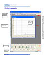
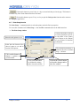
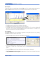
3 - LabSpec5 main window
The main menu bar
The main icons bar
Window of the
active objects
Graphics tools associated
to the active object.
The control panel
The status bar
LabSpec5 manual
7
4 - The main menu bar
The main menu bar is located on top of the LabSpec5 main window.
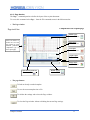
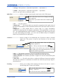
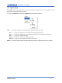
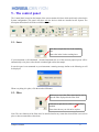
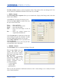
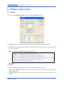
4.1 - File menu
The File commands menu permits to manage the data files and the data printout.
To access the File menu click on the File button of the main menu bar or type Alt+f or Alt+F keys.
Data file management functions
Data printout management functions
Last loaded files
Ø Data file management functions
Open.................................... To open a previously saved object for display.
Close.................................... To close and to remove the current object
Save .................................... To save the current object in a file for later retrieval
Save All............................... To save all the objects of the current window.
Ø Data printout management functions
Print…................................ Output to the default printer.
Print Preview..................... To preview the page before printing.
Print Setup…......................To setup the printer parameters
Page…................................. To define the layout of the page.
Exit...................................... To close and quit the LabSpec5 application.
LabSpec5 manual
8
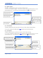
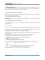
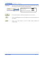
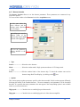
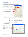
4.1.1 - Open... function
The Open… command permits to select a previously saved file to load it.
To access this command select Open… from the File commands menu in the Main menu bar or use the
keyboard shortcut Ctrl + O or click directly on the following open icon
in the main icons bar.
Select here the folder in which
the file has been saved.
Select in the list of files the
one you wish to load.
Select here the type of
the researched file.
Click on the Open button
to open the selected file.
Click on the Cancel
button to abort the
operation and to close the
window.
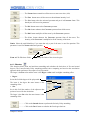
4.1.2 - Close function
The Close command removes the current object of the active window without saving the changes.
To access this command select Close from the File commands menu in the Main menu bar.
4.1.3 - Save function
The Save command permits to record the active object in a file for future retrieving.
To access this command select Save from the File commands menu in the Main menu bar or use the
keyboard shortcut Ctrl + S or click directly on the following save icon
in the main icons bar.
Select here the folder in which
you want the file to be recorded.
List of the files already
existing in the chosen folder.
Enter here the name you
wish to assign to the file.
Select here the file format.
LabSpec5 manual
Click on the Save
button to save the
selected object.file.
Click on the Cancel
button to abort the
operation and to close
the window.
9
4.1.4 - Save All function
The Save All command permits to record all the objects of the active window in a file for future
retrieving.
To access this command select Save All from the File commands menu in the Main menu bar.
Select here the folder in which
you want the file to be
recorded.
List of the files already
existing in the chosen
folder.
Enter here the name you
wish to assign to the file.
Select here the file format.
Click on the Save
button to save the
selected object.file.
Click on the Cancel
button to abort the
operation and to
close the window.
4.1.5 - Print function
The Print… command prints out to the default printer the objects of the active window. The layout page
is the one defined with the Page… command.
To access this command select Print… from the File commands menu in the Main menu bar or use the
keyboard shortcut Ctrl + P or click directly on the following print icon
in the main icons bar.
Print icon
File menu
Print…
LabSpec5 manual
10
4.1.6 - Print Preview function
The Print Preview command allows to display the to-print page before printing.
To access this command select Print preview from the File commands menu in the Main menu bar.
Ø The Print Preview window
The to-print page is displayed in the print preview window as it will appeared at print out so you can
check the page layout before starting the printing operation.
To modify the page layout , use the Page… function of the File menu.
On top of the print preview window some specific buttons commands are available.
Print Preview
specific commands
The to-print page
The Print Preview commands
Click on this button or press P-key or p-key to start the print out.
Click on this button or press N-key or n-key to display the second page in case of a to-print
document on 2 pages. For the moment the layout of a to-print document is only on one page.
Not available. (Future expansion)
Click on this button or press T-key or t-key to display the 2 pages of the document. Useful
for to-print document on 2 pages (future expansion)
Click on this button or press I-key or i-key to zoom the previewed page.
LabSpec5 manual
11
Click on this button or press O-key or o-key to zoom-back the previewed page. This button is
available only if the Zoom function has been activated .
Click on this button or press C-key or c-key to quit the Print preview function and to return to
the LabSpec5 application.
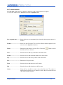
4.1.7 - Print Setup function
The Print Setup… command permits to select the printer and to define its properties.
To access this command select Print Setup… from the File commands menu in the Main menu bar.
Ø The Print Setup window
Click on this button to check
or set the parameters specific
to the model of the printer
used. Report to the manual
of your printer for detailed
information.
Select here the printer to use.
Select here the format of the
sheet of paper to use and its
location in the printer.
The orientation parameter is
linked to the one set with the
Page… function.
Click on this button to
choose a printer on
your network.
Click on the OK button
to validate the settings
and to close the window.
LabSpec5 manual
Click on the Cancel button
to abort the changes and to
close the window.
12
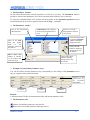
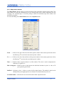
4.1.8 - Page function
The Page… command permits to define the layout of the to-print document.
To access this command select Page… from the File commands menu in the Main menu bar.
➢
The Page window
Components of the to-print page
Page tools bar
Header page
Associated toole:
Each icon allows to
define the size and
the position of each
different predefined
component type of
the to-print page
Data object
Associated tool:
Text object
Associated tool:
graphic object
Associated tool:
Image object
Associated tool:
Information parameters
Associated tool:
➢
Bottom of page
Associated tool:
The page buttons
To load an already recorded template.
To save the current template into a file.
To validate the settings and to close the Page window.
To close the Page window without validating the current Page settings.
LabSpec5 manual
13
Using the Page tools icons
To insert a component in the to-print page click on the corresponding tool. Then move the mouse on the
page so a cross appears. Then move the cross at the wished location, press on the left mouse button and
move the mouse to define the size of the corresponding component.
➢
➢
How to select a component of the to-print page
Move the mouse on the chosen component and click on the left mouse button. Then a dotted rectangle is
displayed around the selected component.
➢
Moving a component of the to-print page
Select the component. Then when the following mouse cursor
drag the mouse.
➢
appears, click on left mouse button and
Re-sizing a component of the to-print page
First, click on the object to select it. Selection handles appear around the selected object.
Move the mouse pointer on one of the selection handles until to have the size pointer:
or
➢
.Keep the mouse button pressed and move the selection handle and modify the size of the object.
Modifying or creating the contents of a to-print page component
Except the data object, the contents of all the other objects could be modified by double-clicking on the
wished component.
Then a dedicated window appears with the tools to modify the corresponding component:
- The options window for the header page, the bottom of page and the Text object.
-The parameters window for the array of experiment information parameters.
-The Open window for the Image object.
➢
Modifying the general page presentation or display
Click anywhere on the to-print page on the right button of the mouse to display the following menu
Cut
To remove the selected component
Format To define the parameters of the sheet of paper. (See Page Setup)
Turn
To define the page orientation Portrait or Landscape
Zoom To define the display of the to-print page inside the Page window.
LabSpec5 manual
14
Ø The Parameters function
On the printed document the selected parameters are laid out in an array. The Parameters function
permits to select the data parameters you wish to be printed and to define the style of the array.
To access this command double click with the left mouse button on the information parameters object
when defining the layout of the to-print document with the Page… command
Ø The Parameters window
List of the non printed
data parameters.
NSParameters tools to manage
the list of the data parameters to
print.
Print list: List of the
data parameters selected
to be printed.
Click on the Style button
to open the NSOptions
window to define the
design of the array.
......in the Title
Enter
field the printed
name
of
the
parameter selected in
the print list
Click on the OK
button to validate the
settings and to close
the window.
Enter
here
the
number of columns
of the printed data
parameters array.
Click on the Cancel
button to abort the
changes and to close
the window.
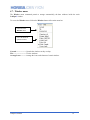
Ø Example of a printed data parameters array
You will find below the data parameters array corresponding to the settings of the parameters screen
copy as it appears on the printed document.
Exposure is the
printed label for
the
exposition
parameter.
Column 1
Column 2
Column 3
Remark:
A column contains 2 fields: the data parameter label and the data parameter value.
Ø The Parameters tools
Add the selected data parameter to the print list.
Remove the selected data parameter from the print list.
LabSpec5 manual
15
In the print list move the selected parameter to the previous line.
In the print list move the selected parameter to the next line.
4.1.9 - Exit
The Exit command permits to close all the opened objects and quit the application.
To access this command select Exit from the File commands menu in the Main menu bar or click on the
Close icon
in the upper right corner of the LabSpec5 main window.
File
menu
Close
button
Exit
LabSpec5 manual
16
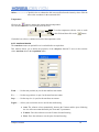
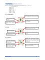
4.2 - Edit menu
The Edit commands menu enables to exchange data between different applications and facilitates the data
analysis process.
To access the Edit menu click on the Edit button of the main menu bar.
Undo (CTRL+Z)....... To undo the last operation.
Redo (CTRL+Y)....... To redo the last operation.
Cut
(CTRL+X).......To cut the active data object in clipboard.
Copy (CTRL+X)....... To copy the active data in clipboard. You can select the data format with the
Format… command.
Paste (CTRL+V)....... To insert the clipboard contents. You can select the clipboard format with the
Format… command.
Format….................. To select the Copy and Paste clipboard data formats.
LabSpec5 manual
17
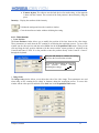
4.2.1 - Format function
This command permits to define the format of the data you export to the clipboard or and the one of the
data you import from the clipboard.
To access this command select Format… from the Edit commands menu in the Main menu bar.
➢
The Copy/Paste data formats selection
In the Copy format
column select the format
of the data exported to
the clipboard.
Click on the OK button to
validate the settings and
close the window
In the Paste format
column select the format
of the data imported from
the clipboard.
Click on the Cancel button
to abort the changes and
close the window.
•
DataNative NextGen format. Can be used to create the exact copy of the data object.
•
TextCreate the text spreadsheet of the active data object.
•
PictureCreate the screen copy picture of the active window.
LabSpec5 manual
18
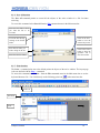
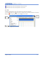
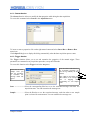
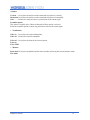
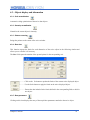
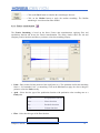
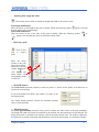
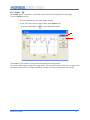
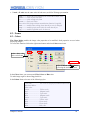
4.3 - Data menu
The Data menu commands permit to activate a data object and to see the list of object of the active
window. This list is shown as a set of color radio buttons on the right pan of the screen.
To access the Data menu click on the Data button of the main menu bar.
You can activate one of the data object of the active window by clicking directly in
the list of the Data menu .
Datas… Select this command to show the full objects list of the active window.
On the following screen
copy the active window
contains 2 objects. (2
spectra) .
You can activate one
object also by clicking
on the colored radio
button.
LabSpec5 manual
19
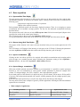
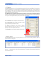
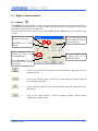
4.4 - Acquisition menu
The Acquisition menu commands permit to setup the data acquisition parameters.
To access the Acquisition menu click on the Acquisition button of the main menu bar.
Custom ..................... To customize the data properties.
Trigger...................... To set the properties of the manual trigger
RTD........................... To set the properties of the Real Time Display acquisition mode.
Options......................To set the parameters of the data acquisition, such as exposure time, binning,
acquisition mode and so on….
Auto save...................To set the ‘Save’ parameters to save automatically the data at end of acquisition.
Multi window........... To set the parameters to define the acquisition spectral regions.
Detector.....................To set the detector properties such as readout zone, gain etc.
Autofocus.................. To set the autofocus properties.
Video......................... To set the video acquisition properties.
LabSpec5 manual
20
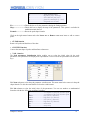
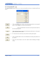
4.4.1 - Custom function
The Custom function allows to modify the data properties table during the data acquisition.
To access this command select Custom in the Acquisition menu.
To insert or remove properties click on the right mouse button and select Insert Row or Remove Row
menu item.
Check Open Dialog box to display this dialog automatically when the data acquisition process starts.
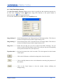
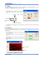
4.4.2 - Trigger function
The Trigger function allows you to set and customize the properties of the manual trigger. These
parameters are common for any acquisition procedure, except in RTD mode.
To access this function select Trigger item in the Acq menu.
In the Start or in the
Sample field you
have the possibility
to customize the
message which will
appear.
You can select at which level of
the acquisition procedure you
need to trig manually the data
readout.
This could be just before each
data readout or for exemple in
case
of
mapping
when
positionning at a new sample
point.
Start .........................Select the corresponding Use box to see the associated message each time the
acquisition starts. You can customize the message text.
Sample ......................Select the Use box to see the associated message each time when a new sample
point is selected for measurement. You can customize the message text.
LabSpec5 manual
21
4.4.3 - Real Time Display function
The Real Time Display Properties Dialog window allows to modify the data acquisition properties for
the Real time CCD-image readout (
Detector image RTD function) or the spectra readout in
adjustment mode (.
RTD function Spectrum )
To access this function select RTD item in the Acquisition menu.
Image binning X ......Set the binning factor in the X direction for the CCD-image readout . This allows to
increase the acquisition speed and the signal intensity level.
Image binning Y ......Set the binning factor in the Y direction for the CCD-image readout. This allows to
increase the acquisition speed and the signal intensity level.
Image zone................ Define here the chip area you wish to load for the RTD CCD-image. You can
choice to read the full chip matrix (select Full) or only the chip area corresponding
to the spectrum readout area (select Spectrum).
Exposition time.........Set here the exposure time value in seconds.. This value appears also in the bottom
control panel.
................... Click on the OK button to validate the settings and to close the window
................... Click on the Help button to retrieve the informations concerning the parameters of
this window.
.................... Click on the Cancel button to close the window without validating the
changes.setting
LabSpec5 manual
22
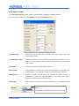
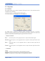
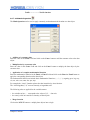
4.4.4 - Options function
The Acquisition Options window allows to define the data acquisition common properties.
To access to this window select the Options item in the Acquisition menu.
Exposition time...................Set here the exposure time value in seconds. This value appears also in the
bottom control panel.
Accumulation number ...... Set here the number of times you wish to repeat the detector exposure.This is
useful in case of signal overflow. This value appears also in the bottom
control panel.
Data name........................... Set here the data label and the default file name
Refresh time........................This parameter is usefull in case of fast acquisition process or big data sizes.
The data display is not refreshed on the screen until this time is elapsed.
Binning factor.....................Define the number of data points per spectrum.The signal intensity is
proportional to this value, but the number of data point (and spectral
resolution) will be reduced in the same way.
Data mode........................... This parameter is used in case of data accumulation ( Accumulation number
>1.)
Click on the down arrow icon to display the Data
mode list
Then select how should be defined the final spectrum
LabSpec5 manual
23
* Average... Final spectrum = ( Spectrum1+Spectrum2+....+Spectrumn) / n
* Summa ... Final spectrum = ( Spectrum1+Spectrum2+....+Spectrumn)
where n is the value of the accumulation number
Spike filter...........................Allows to remove or not the spike cosmic noise of the CCD detector.
Click on the down arrow icon to display the Spike
filter option list
Then select if you wish to remove the eventual spikes
or not.
* Off........... No spike removal
* Double expo........... The cosmic spikes are removed by comparison of the signal values of
the different accumulation. So the accumulation number will be increased on the one time in
this case.
* Single pass..............This method allows to remove spike in a single accumulation
acquisition by analysing bans for sharpness and intensity. This algorithm has to used with
care . Very sharp Raman bands could be modified. Nevertheless this method works fine and
save time when looking broad bands as it is the case for Raman analysis of amorphous
materials or photoluminescence applications....
Autofocus............................ Allows to adapt or not automatically the Z position to obtain a maximal
signal level. The process is based on the detection of the laser beam
reflection.
Click on the down arrow icon to display the
Autofocus options list
In the + field you can adjust the shift value.
Then select if you wish to use or not the Autofocus
and at which step of the acquisition process you wish
to start the autofocus procedure.
* Off........... The autofocus procedure is not used in the data acquisition process.
* Before acquisition. The autofocus procedure is applied before each data readout
* Before each point.. The autofocus procedure is applied at each new measurement point
positionning
* Shift value.............. The shift value allows to adjust the difference between the position
where the laser reflection is at maximum level and the one where the spectroscopic signal is
at maximum level .
Scanning.............................. Allows you to define which scanning device has to be used to record a
spectral image the XY stage or the Scanner.
Click on the down arrow icon to display the X
scanning option list
Then select in the list the wished device.
LabSpec5 manual
24
Use detector ............. On systems with 2 detectors this option allows you to acquire data either from only
the current active detector or from the 2 installed detectors.
Click on the down arrow icon to display the
Use detector list.
Then select the wished option.
............. Click on the OK button to validate the settings and to close the window
................... Click on the Help button to retrieve the informations concerning the parameters of
this window.
.................... Click on the Cancel button to close the window without validating the
changes.setting
LabSpec5 manual
25
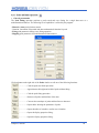
4.4.5 - Autosave function
The Auto Save window allows to modify the properties of the acquisition auto save option.
To access this window select Auto Save item in the Acquisition menu.
Save acquired data............. Select this box to save automatically the data when the acquisition process is
finished.
Format.................................Select here the file format. The list of the different format supported is the
same one as for Open/Save functions.
Folder ................................. Edit here the path where to save the files. Click on the
the folder in the tree structure.
button to select
Year..................................... Select this box to add the year number to the folder name.
Month.................................. Select this box to add the month number to the folder name.
Day.......................................Select this box to add the day number to the folder name.
File....................................... Edit here the file prefix name.
Hour ....................................Select this box to add the hour to the file name.
Min ......................................Select this box to add the minute to the file name.
Count .................................. Select this box to add the counter value to the file name. The counter is
modified each time the auto save function is called. But you can edit the start
value of the counter sequence.
LabSpec5 manual
26
4.4.6 - Multi window function
The Multi Window function allows to set the properties of the acquisition in multi window mode. This
mode enables to record data automatically over an extended range with a defined integration time and
averaging. The extended range is covered by taking a number of individual single shot windows and
'gluing' these together..
To acces this Dialog select Multi Window item in the Acquisition menu.
From.......... Edit here the value of the first limit of the spectral window in the current spectral unit. Select
the following
to activate the associated spectral window.
To............... Edit here the value of the end limit of the spectral window in the current spectral unit. Select
the following
to activate the associated spectral window.
Time........... Edit the relative exposure time(in %) of this window. This value is used to compensate the
differences of signal level.
Min overlap (pix)..... Define here the overlap between the individual windows in pixels. A value of 50
gives generally good results.
SubPixel.....Selecting a value >1 allows to restore the fine shape features. The method is based on the
shifting of the spectrograph position on a distance less than the detector pixel size.
Use multi window.....Select this box to activate the multi window acquisition mode
LabSpec5 manual
27
Auto overlap............. Select this box to automatically define the overlapping size.
Merge data................Select this box to create one data object for each active spectral window. In the
other case a data object is generated for each spectral range corresponding to the spectrograph position.
Adjust intensity........ Select this box to adapt the intensity to the same values on the overlapping parts.
This adaptation is based on the linear shift of the data.
................... Click on the OK button to validate the settings and to close the window
................... Click on the Help button to retrieve the informations concerning the parameters of
this window.
.................... Click on the Cancel button to close the window without validating the
changes.setting
LabSpec5 manual
28
4.4.7 - Detector function
The Detector function allows to set the detector parameters. These parameters are common for any
acquisition process.
To access to this window select Detector item in the Acquisition menu.
In this part select the
active detector and the
readout mode (Spectrum
or CCD image)
In the Sizes part enter the
readout limits of the
detector chip for the mode
selected in the Type part.
Set here the parameters
options attached to the
detector.
➢
Type
Sensor........................ Select the active detector.
Mode..........................Select the readout mode. Single spectrum readout or CCD image mode.
➢
Sizes
Sizes........................... Edit the readout limits of the detector chip. To check the readout zone run the
detector image Real Time Display, by clicking on the
icon.
➢
Options
This section groups together parameters specific to the detector model. So this section appears differently
following the model of the installed detector. The most commonly used parameters will be described
hereafter. It is possible that some parameters does not appear if the correponding option is not available
on the on your current detector.
High speed................ Check this box to enable high speed data transfer.
High gain...................Check this box to enable high gain level of the detector amplifier.
LabSpec5 manual
29
Offset ........................Check this box to subtract the dark current offset from the intensity values. Edit the
offset value to subtract in the associated field.
Temperature
Click on the
button to capture the current detector temperature.
The current temperature read is displayed in this field.
To set the temperature edit the value to reach
in this field and then click on the
button.
Check this box to have a continuous refresh of the temperature value.
4.4.8 - Autofocus function
The Autofocus ensures an optimal focus is reached before an acquisition.
This function allows you to define the properties of the Autofocus function.To acces to this window
select Autofocus item in the Acquisition menu.
From.......... Set the start position (in μm) for the autofocus movement.
To............... Set the stop position (in μm) for the autofocus movement.
Step ........... Set the step size (in μm) for the autofocus movement.
Engine........ Allows you to select the device used for the autofocusing

Auto: The software select automatically between the Z-motor and the piezo following
the size of the movement defined by the From and To parameters.

Z-motor: Force the software to use the Z-motor for autofocussing

Piezo: Force the software to use the piezo for autofocussing.
LabSpec5 manual
30

Z-motor & piezo. The software uses the both devices for autofocusing. A first approach
is done with the Z-motor. The research of the final position is then refined by using the
piezo.
Intensity.....Display the autofocus diode intensity.
..Validate the settings and close the Autofocus window.
.... Close the Autofocus window without validating the setting.
4.4.9 - Video functions
Laser Position
The Laser Position window allows you to modify the position of the laser beam on the video image.
These parameters are used when the XY scanning is used during the acquisition process. To access this
window run the video preview and then select Laser item in the Acquisition/Video menu. Then you can
click and drug the laser position indicator with the mouse and the current position is refreshed in the
CenterX and Center Y field . It is also possible to enter the position directly in the CenterX / Center Y
through the keyboard.
➢
Click the OK button to validate the settings
and Close the Laser Position window.
Click on the Cancel button to close the
Laser
position
window
without
validating the settings.
Image Scale
The Image scale window allows you to adjust the scale of the video image. These parameters are used
when using an XY scanning device (Stage or Scanner) during the acquisition process. To access this
window run the video preview and then select Scale item in the Acquisition/Video menu.
➢
LabSpec5 manual
31
Corner points Move the XY stage to left-up rectangle corner and click on the point #1. Then move stage
to right-bottom corner and click on the point #2. Program will read the stage position and use this values
as rectangle sizes.
SizeX
X size of the rectangle.
SizeY
Y size of the rectangle
Stage
Click on the button to modify video scale, used by XY stage. This operation
should be done for each microscope objective.
Scanner
Click on the button to modify scanner scale.
Clear
Clears SizeX and SizeY fields for stage joystick operation.
LabSpec5 manual
32
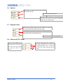
4.5 - Option menu
The Option menu commands allows to select the default working unit and to convert the active data
object to the selected units when necessary.
To access the Option menu click on the Option button of the main menu bar.
Unit........ Select this command to modify the default spectral and intensity units.
Nm............. To give the frequencies in nanometer (Wavelength spectral unit)
1/cm...........To give the frequencies in cm-1 (Raman shift (relative wavenumber) spectral unit)
Cnt.............To give the intensity in Counts.
Cnt/sec...... To give the intensity in Counts per second.
Convert..... To give the active data object in the selected units.
Multi...... Select this option to apply any data treatment operation to all the data of the active window.
LabSpec5 manual
33
4.6 - Setup menu
4.6.1 - Instrument
This function allows you to setup the instrument following the needs of the measurement and the
configuration of the instrument.
Actually this function is available only for the Aramis system.
To access this function select Instrument item in the Setup menu.
The Aramis window is organized by functions: Measure localisation, Polarization, Visualization,
Measure. The software checks the presence of the different motors and their position. So if a motor is not
present the corresponding commutation appears in gray and could not be selected.
➢
Measure Localization
Retro ......... Select this oprion to set the appropriate mirror to capture the Retro-Raman signal
Macro 90....Select this option to set the appropiate mirror to capture the raman signal from the macro
plate.
Micro..........Select this option to set the appropiate mirror to capture the raman signal from the
microscope.
External..... Select this option to set the appropiate mirror to capture the raman signal from the fiber
input.
➢
Polarization
* Laser
Vertical...... Setup the λ/2 slide to obtain a vertical polarization of the laser.
Horizontal. Set in place the optical to retrieve the natural polarization of the laser.
Circular..... Set in place the λ/4 slide to obtain a circular polarization of the laser.
LabSpec5 manual
34
* Raman
Vertical...... Set in place the analyser on the raman path to polarize it vertically.
Horizontal. Set in place the analyser on the raman path to polarize it horizontally.
None........... Remove the analyser to have no polarization of the raman signal.
Scrambler option.
This option is available only if Retro or Macro90 or Micro option is selected.
Select the scrambler option to cancel any polarization effect on the raman signal.
➢
Visualization
Video on ....Set in place the camera beamsplitter.
Video off ... Remove the camera beamsplitter
Trino off.... Set in place the trino for the selected option.
Trino on
Trino FTIR
➢
Measure
Point mode Set in place the pinhole and the lenses assembly following the selected measure mode.
Line mode
LabSpec5 manual
35
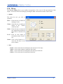
4.7 - Window menu
The Window menu commands permit to arrange automatically the data windows inside the main
LabSpec5 window.
To access the Window menu click on the Window button of the main menu bar.
Functions of the
Window menu
List of the different
opened windows.
Cascade.........................Cascade the windows so they overlap.
Tile................................ Tile the windows.
Arrange Icons.............. Arrange the icons at the bottom of a main window.
LabSpec5 manual
36
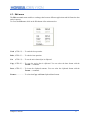
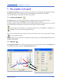
5 - The control panel
The Control Panel located on the bottom of the screen contains divisions which are directly related to the
System configuration. This panel will show only the devices which are installed on the System. The
description below details all of the available sub-units.
5.1 - Laser
Click here to open the list of the installed
laser.
Then select in the list the working laser.
If your instrument is full automated ( Aramis instrument) the set of the necessary optical pieces will be
automatically set in place so the chosen excitation light reaches the sample.
In case this part is not automated on your instrument a warning message similar to the following on will
be displayed.
When everything is in place, click then on the OK button.
5.2 - Filter
Click here to reset the filter wheel and to set in
place the filter displayed in the filter field.
Click here to open the list of the 6 neutral filters
installed.
Then select the one you wish to be in place.
Note: The reset function of the filter wheel is usefull when for any reason the selected filter is not well in
place or does not match the selected one.
LabSpec5 manual
37
There are 6 neutral filters installed with the optical densities 0.3, 0.6, 1, 2,3 or 4.
[...] = no attenuation (P0)
[D0.3] = P0 /2
[D0.6] = P0 /4
[D1] = P0 /10
[D2] = P0 /100
[D3] = P0 /1000
[D4] = P0 /10000
5.3 - Confocal hole
Initialize the confocal hole by closing the
hole and opening it to the previous value.
Close the confocal hole
aperture.
Set here the value of the
aperture of the confocal
hole
5.4 - Slit.
Open the confocal hole to the maximum
value of aperture.
Initialize the slit by closing the slit and
opening it to the previous value.
Close the slit.aperture.
Set here the value of the
aperture of the slit.
5.5 - Spectro
Move the spectrograph
grating to the zero order
position. (0nm)
Enter here the spectrograph
grating position value in
the active spectral unit.
LabSpec5 manual
Open the slit to the maximum value of
aperture.
Initialize the spectrograph grating
position. Move to the zero order position
and then move to the position value
previously set.
Move the spectrograph grating to the
highest value of position.
38
5.6 - Options
Click here to select one of the available
spectrograph gratings
Select the microscope objective.
Enter here a name for the next recorded spectral
data object. The software will add an incremental
number after the entered name.
5.7 - Exposure times
Enter here the exposure time value in seconds to be used for
the spectrum and image RTD acquisition mode
Enter here the exposure time value to be used for the spectrum
and spectral image accumulation mode.
Enter here the number of accumulations.
5.8 - Motorized XY/Z Table
Position of the different axis
of the motorized XY/Z table.
Enter here also the position
you want the table to be
moved.
LabSpec5 manual
Select the small blank box attached to
each table moving axis to have the
corresponding position value refreshed in
real time even when moving with the
joystick.
39
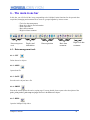
6 - The main icons bar
In this bar you will find all the icons correponding to the LabSpec5 main functions for the spectral data
acquisition, managing and treatment.These icons are grouped together by interest center.
Display and
information
Data acquisition
Basic data
treatment
{
Data management
tools
{
{
{
{
* Tools for data management
* Data object display and information.
* Data acquisition
* Basic data treatment
* High-level data treatment
High level data
treatment
6.1 - Data management tools
6.1.1 - CUT
Delete the active objects.
6.1.2 - OPEN
Open a data file.
6.1.3 - SAVE
Save the active objects into a file.
6.1.4 - PRINT
Print to the current printer the active to-print page. For more details please report to the description of the
print , print preview, print setup and page function in the File menu chapter.
6.1.5 - HELP
Open the LabSpec5 Help index.
LabSpec5 manual
40
6.2 - Objects display and information
6.2.1 - Scale normalization
Automatic scaling optimization of the active data objects.
6.2.2 - Intensity normalization
Normalize the current object in intensity.
6.2.3 - Pointers centering
Brings the pointers to the center of the active window.
6.2.4 - Data sizes
This function reports the limits for each dimension of the active object in the following window.and
allows you to re-define it if necessary.
The Size field reports the number of the spectral points for the correponding axis.
..............Click on the Get button to update the limits of the current active displayed object.
..............Use the Scale button to apply the limits to the active displayed object.
..............Extract the data included in the limits defined in the corresponding fields to build a
new object..
6.2.5 - Data parameters
Clicking on this icon displays the array of the acquisition parameters attached to the active object.
LabSpec5 manual
41
6.3 - Data acquisition
6.3.1 - Spectrum Real Time Display
The main purpose of this function is to offer a tool to allow you to adjust quickly the focus and the other
experimental conditions to maximize the Raman signal. Clicking on this icon starts in continuous the
following cycle:
- Acquisition in single shot window of a spectrum.
- Display of the acquired spectrum.
Each spectrum displayed replaces the previously displayed spectrum. There is no averaging or spectra
accumulation and no extended coverage possible. For this use the dedicated accumulation functions
described below.
The exposure time used is the one set in the RTD exposure time field in the control panel (Report to the
exposure time section in the control panel chapter).
The CCD pixels read are the one set in the Acquisition / RTD function.
To stop the continuous readout click on the STOP icon located at right end of the main icons bar.
6.3.2 - Detector image Real Time Display
The purpose of this function is the same as the one described in the pevious section applied to the CCD
image.
The CCD image is a 2D image of the intensity of each pixel of the CCD chip. Following the parameters
set in the Acquisition / RTD function this could be the full chip but also a part of the chip.
6.3.3 - Spectra accumulation
Clicking on this icon allows spectra to be acquired with multiple accumulations and averaging and/or
with coverage over extended spectral ranges following the parameters setting of the Acquisition /
Detector function , the one of the Acquisition / Multi window function.
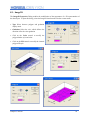
6.3.4 - Spectral Images accumulation
With some suitable optional accessories installed on your instrument it is possible to acquire spectra in
function of one or a combination of some specific variable parameters to obtain for example XYZ
volume, XY mapped images, line (X/Y), depth (Z) , time and temperature profiles.
So the main purpose of this function is to acquire an array (3D for volume, 2D for map or 1D for profile)
of spectra, with each spectrum acquired with specific variable parameters like for example position, time,
temperature...
In all cases the result spectral array is saved in one single file for fast and easy data analysis.
The array below shows some examples of general possible applications following the different additional
optional dveices innstalled.
➢
Main examples of applications
Variable parameter
Results
Optional device used
X or Y position
Line profile
Motorized XY table / Scanner
Z position
Depth or Z profile
Motorized Z motor / Piezo
LabSpec5 manual
42
Variable parameter
Results
Optional device used
Time
Time profile
No additional device
Temperature
Temperature profile
Heating/cooling stage
X and Y position
Map
Motorized XY table
X,Y and Z positions
Volume
Motorized XY/Z stage or
Motorized XY stage and piezo
6.3.5 - Spectral Image properties
6.3.6 - Multi window
Clicking on this icon allows you to define the properties of the spectra acquisition over extended spectral
ranges. You can also acces to this function from the main menu bar . Acquisition / Multiwindow. So
please report to this section for detailed explanations.
6.3.7 - Video
Clicking on this icon starts the continuous video image grabbing. To freeze the image press on the STOP
icon located at the right end of the main icons bar.
6.4 - Basic data treatment
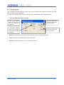
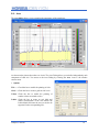
6.4.1 - Baseline correction
Clicking on this icon allows you to access the baseline correction functions.
The Baseline correction performs baseline correction of data by using a manual or automatic approach
and converts baseline profile to data array.
LabSpec5 manual
43
➢
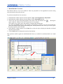
Manual Baseline Correction
The Manual Baseline Correction method is based on polynomial or line-segmented correction using
referenced points selected by the user.
To perform a manual base line correction :
1. In the Baseline window options select the baseline Type : Line Segmented or Polynomial.
2. In the Baseline window options select the Degree for the Polynomial baseline.
3. Then in the left object associated graphics tools panel select the Baseline tool .
Moving the
mouse inside the window of the active objet moves a cross pointer.
This enables you to add or move the points by clicking at the desired place.
By setting the Attach parameter in the options of the Baseline window to Yes the selected baseline
points are attached to the spectrum data.Setting this Attach parameter to No allows you to freely place
the points anywhere in the window.
4. In the Baseline window options use the Style list to select the style to display the baseline calculated
from the selected points.
5. Click on Sub button to subtract the baseline from the data.
This operation could be applied to multidimensional data set, visualized in one-dimensional curve mode
(1D)
Move this cross pointer and
click at the wished place to
define the baseline points
LabSpec5 manual
44
The baseline is displayed
in the selected style.
➢
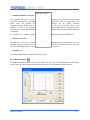
Automatic Baseline Correction.
The Automatic Baseline Correction
(non-peak) of the data. The algorithm
points above the baseline are
continues until the fitting errors are
number of points is not changed.
The baseline is then automatically
is displayed.
iteratively fits a polynomial to the baseline
starts with a full set of data points. The
removed and the fitting procedure
less than the predefined value or the
Click on Auto button to start the procedure.
subtracted from the data and the finalresult
To calculate the baseline without
subtraction, click on the Fit button.
➢
Baseline Conversion.
The Baseline Correction operation
operation allows the baseline trace to
Click on the Convert button to start
➢
replaces the data by the baseline trace. This
be saved as a data file for future retrieving.
this function.
Baseline Clear.
Click on the Clear button to remove the baseline points.
6.4.2 - Data correction
The Data correction function allows you to modify all the traces of a multidimensional data matrix.
Some of these operations require an additional spectrum as a second parameter of the operation.
LabSpec5 manual
45
............. The Norma button normalizes all the traces to same area value (100).
............. The Zero button moves all the traces to the minimum intensity level.
............. The Get button takes the activated spectrum and put it in Corrector frame. This
data object will be used as parameter.
............. The Del button removes the Corrector spectrum.
.............The Sub button subtracts the Corrector spectrum from all the traces.
..............The Mul button multiplies all the traces by the Corrector spectrum.
..............The Corr button subtracts the Corrector spectrum from all the traces. The
intensity of the Corrector is multiplied to fit the intensity of the trace
Limits Select the small blank box if you want that only a part of the trace is used for operation. This
parameter is used for Norma and Corr operation.
From and To Edit these fields
to modify the limits of the selected region.
6.4.3 - Filtration
This function allows linear and non-linear smoothing and calculates the derivatives of first and second
degrees. The Linear Savitsky-Golay smoothing and derivative computing are based on the convolution
approach which performs a least squares fit of polynomial.
The larger is the Size value and the lower is the Degree value result in a higher smoothing effect.
➢
Degree
Set in this field the degree of the polynomial.
The lower is the degree the more intense is the
smoothing effect .
➢
Size
Set in this field the number of the adjacent data
points to be used for the calculation.
The larger is the Size value the more intense is the
smoothing effect
.............. Click on the Smooth button to perform the Savitsky-Golay smoothing.
.............. Click on the Der 1 button to calculate the first degree derivate.
LabSpec5 manual
46
.............. Click on the Der 2 button to calculate the second degree derivate.
.............. Click on the Median button to apply the median smoothing. The Median
smoothing is a non-linear data filter method.
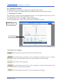
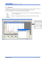
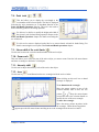
6.4.4 - Fourier transformation
The Fourier Smoothing is based on the direct Fourier data transformation, applying filter and
apodization function and inverse the Fourier transformation. The dialog window shows the real and
imaginary Fourier functions and allows you then to select the smoothing property.
➢
Limit – Enter in this field the position of the cutoff point in %. This parameter defines the smoothing
factor 0 – full smoothed, 100 – no smoothing. Click on the GO button to apply the value or drag the
pointer to select the Limit visually.
➢
Apod – Select here the type of the apodization function with apodization value reaching zero at a
Limit point.
None........................... No apodization function
Line............................ Linear function
Sqr ............................ Parabolic function
Cos............................. Cosinus function
➢
Filter –Select here the type of the filter function.
None ..........................No filter function
LabSpec5 manual
47
Traffic .......................Traffic function
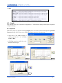
6.4.5 - Arithmetical operation
The Math Operation can be used to apply commonly used mathematical formulas to a data object.
Addition of a constant value
Enter the value in the Const+ field and click on the Const+ button to add the constant value to the data
object.
➢
Multiplication by a constant value
Enter the value in the Const* field and click on the Const* button to multiply the data object by the
constant value.
➢
Application of a complex mathematical function
Enter the mathematical function in the Func1 or Func2 fields and click on the Func1 or Func2 button to
apply the correponding function to the data object.
The mathematical formula can include basic mathematical function (+, -, *, /, ^), negating, pow, log, exp,
sin, cos, asin, acos, atan, abs, sqrt, step.
➢
For example the “sin(a)” formula replaces the data intensities by sinus function.
The “1000*log(abs(x)+1)” converts intensity to logarithm scale.
The following rules are applied for the variables names:
–
–
the variables a, b, c, … correspond to the values of 1,2, … data axis
the x and y value are consider as intensity of data objects.
➢
Merge function
Click on the MERGE button to multiply data objects into a single.
LabSpec5 manual
48
6.4.6 - Peaks and Bands operations
General presentation
The Peak Fitting operation performs a peak search and curve fitting for a single data trace or a
multidimensional data set. The following list of capabilities is offered by the program:
➢
- Manual or Auto peak selection routine.
- Gaussian, Lorentzian, Polynomial and other mathematical formulas for peak.
- Fixing peak parameters during curve fitting operation.
- Mapping peak parameters for multidimensional data matrices.
Click on button on the right side of the Peaks window to call one of the following functions:
.................. Calls the peak auto finder procedure.
..................Αpproximates the height and width of peaks without fitting.
...................Calls the peak fitting procedure.
..................Removes all peaks and baselines of the data.
...................Converts the sum shape of peaks and baselines to data trace.
...................Οpens tables showing the parameters of peaks.
..................Οpens the tables of variables, used in curve formulas.
..................Οpens the display properties dialog.
..................Opens the display properties dialog.
LabSpec5 manual
49
Peaks selection
The Peak Edit Properties control the automatic and manual peak correction.
➢
Select or edit Peak Shape control to modify the
peak curve shape. This value will be used, when
you insert a peak manually or call the peak Search
procedure.
Edit the Search Min Level box to modify the
parameters level for the peak Search algorithm.
Edit the Search Size box to modify the number of
points for the peak Search algorithm.
To select and define peaks manually use the following icons on the left graphics tool panel.
........................... To add or move a peak
...........................To adjust the height and width of a peak.
............................ To remove a peak.
•
Adding or moving a peak.
Click on this icon.
Then move the cross at the desired
position. A peak will appear in
function of the settings of the SHOW
properties.
LabSpec5 manual
50
•
Adjusting peak height and width
Click on this icon to define or modify the height and width of the selected peak.
Peak height modification
Move the mouse on the height of the peak to modify. When the following symbol
appears click and
drag the mouse to the wished height.
Peak width modification.
Move the mouse on one of the sides of the peak to modify. When the following symbol
or
s cli appears click and drag the mouse to obtain the wished width.
•
Removing a peak
Click on this
icon to remove
peaks.
Move the mouse
pointer on the peak
you wish to remove.
When the following
symbol
appears
click on the left
mouse button. The
correponding peakk
is removed.
➢
SEARCH function
The Peak Search operation performs a search for peaks. It iterates all the points of the data trace to
localize the local maxima.
In the Search Size field define the number of points in the
maximum locality.
The Search Level parameter controls the minimum intensity
value of local maximum.
APPROX function
The Peak Approximation procedure can be used to estimate the initial values of the peak parameters.
The height and width of the peaks are modified by this method; the other parameters are not changed. The
height of the peak is replaced by the intensity value at the peak position point. The width is replaced by
the difference in position of the peak and the intensity value of the nearest point, less then half of height.
➢
LabSpec5 manual
51
FIT function
The Peak Fit algorithm uses the Levenberg-Marquart method of non-linear peak fitting. It is based on the
iteratively adjustment of every peak parameter to attempt the minimal value of χ2. The basic problem of
such an approach is that it can be the multitude of possible solutions and depending on the starting values
of peak parameters. To avoid such a situation you should select the position and shape of the peak as
much to presumed solution as possible.
The Approx procedure allows the initial values to be adapted to the intensity of data points around the
peak. The other way is to fix the parameters which are known. You can select the maximum number of
iteration to limit the treatment time. Increasing the number of skip data point allows to check quickly the
convergence of the algorithm and the quality of the initial value selection.
➢
Edit the Iteration field to modify the maximum iteration.
Edit the Skip point field to modify the number of data
points skipped from the fitting procedure.
The Error box displays the error value, as distance
between original data and curve sum of all peaks and
baselines. This value is named usually as χ2.
Check Baseline box to fit baseline together with the peaks.
PEAKS... function
The Peak Table dialog shows the peaks parameters. You can edit each of these parameters, add new
peaks and remove existing ones.
➢
p, a, w… columns show the values of the peak parameters. The number of the parameter depends from
the peak shape formula.
LabSpec5 manual
52
p................................. peak position (cm-1)
a..................................amplitude (max. Intensity)
w.................................full width half max (cm-1)
g..................................gaussian contribution (1= max)
s ................................. integrated area of band
Fix ............................. Check this box to fix the parameters during the fitting operation
Map .......................... Check this box to display the map of the parameters. This option is available for
multidimensional data set.
Formula ................... Shows the peak shape formula.
Click on the right mouse button and select Insert row or Remove row menu items to add or remove
peaks.
CLEAR function
Remove all peaks and baselines of the data.
➢
CONVERT function
Convert the sum shape of peaks and baselines to data trace.
➢
VAR... function
The Peak parameters Initialization dialog enables you to select the initial value for the peak
parameters. The parameters are displayed in a spreadsheet. To move inside the spreadsheet use the arrowkeys.
➢
Edit Name column to select the peak parameter variable name. This name must be the same as in the peak
shape formula. To edit the name double click on the variable name.
Edit Init column to select the initial value of the parameters. You can use number or mathematical
formulae with the the following predefined variables:
x .................................x coordinate of the peak insertion point
y..................................y coordinate of the peak insertion point
minx........................... low limit of x data axis.
maxx.......................... high limit of x data axis.
miny........................... low limit of y data axis.
maxy.......................... high limit of y data axis.
dx................................maxx-minx
dy............................... maxy-miny
LabSpec5 manual
53
Edit Min and Max columns to select the parameter limits. These limits will be used during the fit. You
can use number or mathematical formulae in the same way as for Init.
SHOW... function
The Peak Fitting Show Properties allows you to customize the display of the fitting results in the data
object current window.
➢
Check Show box to display the following items.
Click on the Style control to modify and select
the style of the selected item.
Text ........... shows peak label.
Arrow ........shows the peak arrow stick.
Shape .........shows the band shape.
Sum ........... shows the result shapes of the all
bands.
Res .............shows the residual between the
original data and band sum.
Check Use data style to control the use data color
when drawing the peak tick and label. In other
cases the Arrow and Text styles will be used.
Check Shape multicolor box to personalize the
color for each peak.
Check Attach arrow box to show the peak label
tick immediately above data shape.
SHAPES... function
The Peak Shapes allows to customize the shape of the peak.
➢
Edit the shape Name in the left
column. This name will then
appear in the list of the available
peak shapes of the Shape item in
the Peaks window.
Edit then the corresponding
mathematical Formula in the
Formula column. Some of the
formula parameters have a
predefined meaning :
• a peak amplitude
• w peak width
• p peak position
Then use the peak parameters initialization function (VAR... button) dialog to set or modify the initial
value of these parameters.
LabSpec5 manual
54
6.4.7 - Profile
The Profile operation performs a visualization of the vertical or horizontal profile of an image.
To start a Profile operation :
•
Load an image and activate image display window.
•
Select cross line pointer by using window menu Pointer item.
•
Click on the following icon
to open the profile window.
Choose Hor or Ver control to select between horizontal and vertical profiles.
Click on the Corr button to replace the image profile. This operation can be useful when you apply some
operations to the profile (for example smoothing) and then you want to set data back to the image.
LabSpec5 manual
55
6.5 - High level data treatment.
6.5.1 - Mapping
The Mapping procedure generates a map by using the signal intensity in the selected spectral regions. Up
to 4 maps can be displayed when you load or acquire the spectral image: the first three are the average
signal intensity and the last is the signal ratio.
The selection of the spectral region is done with the Red, Green or Blue pointer in the spectral image
window.
Check Use box to generate
the corresponding map.
Check Base box to subtract
baseline.
Check Green/blue box to
generate the map of the
corresponding ratio.
You can edit From and To
fields to adjust the limits of
the spectral regions.
Click on the Correct button
to modify data on the
selected data point(s).
Check Spectrum box to see
the spectrum of the selected
data point(s) .
.................Click on the OK button to generate the map following the settings and close the
mapping window.
................ Click on the Convert button to convert the current map into spectral image and
close the mapping window.
.................Click on the Help button to retrieve the informations concerning the parameters of
this window.
................. Click on the Cancel button to close the Mapping window without without
validating the changes.setting
LabSpec5 manual
56
6.5.2 - New spectral profile
The Spectral Profile operation allows you to create and modify the all traces of spectral profile data
matrix.
................................... Click on the NEW button to take the activated spectrum and create a new spectral
profile . Edit the Name box to define the spectral profile.
............
Click on the Add button to take the activated spectrum and add it to
the end of spectral profile.
................................... Click on the Insert button to take the activated spectrum and insert it to the spectral
profile, selected by cursor pointer.
........... To removes the trace selected by cursor pointer from the spectral profile.
................................... Click on the Help button to retrieve the informations concerning the parameters of
this window.
................................... Click on the Cancel button to close the window without validating the changes
setting.
LabSpec5 manual
57
6.5.3 - Modeling
Click on Modeling icon to open DCLS Dialog.
The Direct Classical Least Squares finds the linear combination of data from pure components making up
the combination that most closely matches the original data. This operation, applied to all traces of the
original data sets, yields the maps of each component. The multiplicative constants used on the pure
spectra are proportional to the concentrations of respective components. The difference between the
sample and the linear combination is the residual spectrum, which could be useful for diagnostic
purposes. DCLS requires the spectra of all components presented in the sample, and assumes that this
spectra are not the changed when the component are mixed together. To apply DCLS mapping :
•
Activate the multidimensional Data Matrix
•
Click on the
•
•
•
Activate the Spectrum window
Enter Model Name.
Click on New button to use the spectrum as Model.
icon to open DCLS Dialog.
If you choose Allow negative scores check box, the program
will use any type of combination, even if this combination
includes negative values. Such a combination corresponds to
negative concentrations that do not have a physical sense. This case often happens when the set of
component are not completed or a contribution of some components is near to zero.
Select Show error map to see the distribution of the error.
LabSpec5 manual
58
7 - The graphics tools panel
The graphics Tool Panel on the left part of the screen allows you to modify the data appearance and run
visual edit operations. Following the type of the current data object the tool panel is updated.
You will find hereafter a description of all the tools available.
7.1 - Activate the pointer
The Pointers permit you to check the coordinates of the data matrix axis at the desired location.
To activate a pointer click on the pointer icon in the graphics tools bar (left bar).
To change a pointer position click with the left mouse button and drag to the wished position. The current
pointer coordinates are displayed in the status bar at the bottom of the main window.
If the current active data object is a 2D spectral image click on the SpImRed, or SpImGreen or
SpImBlue icon to activate the corresponding pointer.
In any case to initialize the pointer position (move to the window center) click on the pointers centering
icon in the main icons bar.
LabSpec5 offers also the possibility to customize the pointers display by using the pointer function of the
Window context menu.
7.2 - Integral
The Integral Operation can be used to calculate the area of a spectrum peak. Click on the Integral icon
in the graphics tool panel to open the Integral Operation dialog.
LabSpec5 manual
59
From..........................Edit here the the low integral limit. You can also drag the pointer to select the limit
interactively
To...............................Edit here the high integral limit. You can also drag the pointer to select the limit
interactively
Top.............................Shows the integral result without baseline.
Base........................... Shows the baseline value
Full............................ Shows the Top + Base value.
Format...................... Select here the number of digits to display the result numbers
Line ...........................Click on the control to modify the color and line style.
Fill..............................Click on the control to modify the color and style of the background.
Click on the Apply button to apply the From, To, Line and Fill settings.
Click on the Copy button to copy the values to the clipboard. This is usefull to retrieve these
values by using Copy/Paste functions from other softwares.
7.3 - Baseline
Use this tool to define the points to build the baseline to perform a manual baseline correction.
Moving the mouse inside the window of the active objet moves a cross pointer. This enables you
to add or move the points by clicking at the desired place.
Use this tool to remove some points of the baseline. Move the mouse inside the window of the
active object on the point you wish to be removed. When the square cursor appears click on the
left mouse button to remove the wished point.
7.4 - Manual contant multiplication to data
Use this tool to multiply by a constant the active spectrum. This a manual method using the mouse. Press
the Mul const icon and move the spectrum up or down to the wished position.
7.5 - Manual constant addition to data
Use this tool to add a constant to the active spectrum. This a manual method using the mouse. Press the
Add const icon and move the spectrum up or down to the wished position.
7.6 - Remove ‘spike’
Use this tool to remove no desired points like spikes , cosmics rays,...
7.7 - Correct data shape
This tool allows you to modify a spectrum by correcting each point of the spectrum.
LabSpec5 manual
60
7.8 - Peak tools
This tool allows you to display the wavelength or the
wavenumber of the selected peaks. The label is displayed
following the style parameters set in the show function of the
Peaks and Bands operations function. This tool is also used to
define manually peaks for the fitting operation.
Use this tool to define or modify the height and width of
the selected peak for band fitting operation. Report to the
Peaks and Bands operations chapter for details concerning the
use of this tool.
Use this tool to remove displayed peaks label or to remove bands selected for bands fitting. For
details concerning this tool report to the Peaks and Bands operations chapter.
7.9 - Linear shift of the scale limits
Use this tool to move the vertical or/and horizontal of the active object.
7.10 - Zoom scale
This tool allows you to select the part of the active object you want to zoom. Press the left mouse button
and draw a rectangle to define the wished part.
7.11 - Intensity shift
Use this tool to adjust the intensity scale of the active data object.
7.12 - Axes
Use this tool to position and dimension the axes rectangle inside the active window.
When clicking on this tool icon a dotted
rectangle is displayed.
To re-dimension the rectangle:
Move the mouse pointer on one of the
selection handles until to have the size
pointer: or
.Keep the mouse button
pressed and move the selection handle to
modify the size of the axes rectangle.
To move the rectangle:
Move the mouse pointer anywhere inside
the rectangle . When the moving pointer
appears press the left mouse button and drag to move the rectangle inside the active window.
LabSpec5 manual
61
7.13 - Change 3D axes.
LabSpec5 manual
62
8 - Window context menu
8.1 - Format
You can open Vizualization Format dialog by selecting Format menu item
➢
Internal Click on this control to modify the color and style of the data field background
➢
External Click on this control to modify the color and style of the window border. Usually it is where
the axes are painted.
➢
Mode
Select one of the following data display modes
Single..........only activated data object is displayed
Overlay...... all data objects are displayed on the same place
Tile..............data objects will be shown in the separated rectangles
Projection.. trace of the activated data object will be shown in the separated rectangles
Trace.......... single trace of the activated object will be shown.
Use the right scroll bar to change the trace.
Dimension
1D / 2D 3D
➢
➢
Use scroll scale check this box to use the window bottom and right scroll bar
Always show scroll bar check this box to always show the scroll bars, when the visual zone is large
then the data limits.
➢ One data per view if you check this box, the next time data is displayed a new window will be
created.
➢
LabSpec5 manual
63
➢
Y scale = X scale uses the same scale for both axes; useful for 2D image presentation.
Scale .......... shows the scale properties for each of the window axes.
From ..........value of low axis limit
To ...............value of high axis limit
Freeze ........fixes axis limits.
The scale will be skipped when normalization function is applied.
Auto ...........enables auto scaling when data object axis is changed
Prop ...........enables proper scale limits for each data object.
Log .............enables logarithm scale for the axis
8.2 - Norma
8.3 - Colors
The Colors Dialog enables the image color properties to be modified. Such properties are used when
displaying images.
To access this function click on the right mouse button and select Colors menu items.
Select here the
active color frame
Adjust Contrast and Brightness
by moving the scale bar cursors.
In the Colors frame you can turn on/off Red, Green or Blue color.
To make image negative choose Neg check box.
In the Palette frame select one of the following styles:
True color................... All colors are displayed without modification
Black and White.
False color.
Green ......................... Yellow scale.
Red ............................ Magenta scale.
Blue ........................... Cyan scale.
Blue ........................... Magenta scale.
Green ......................... Cyan scale.
Red ............................ Yellow scale.
Blue ........................... Green scale
Red ............................ Green scale.
Blue ........................... Red scale.
LabSpec5 manual
64
8.4 - Axes
The Axes dialog allows you to customize the appearance of the graph axes.
As shown on the picture above there are 4 axis. The Axes Dialog allows you to define independently each
component of each axis. You access to the Axes Dialog by selecting the Axes item of the window
context menu.
➢
Options
Tick ...... Check the box to enable the painting of ticks.
Grid.......Check the box to create a grid for tick levels.
Values .. Check the box to enable the painting of
number values associated to ticks.
Labels .. Check the box to create an axis label and
enable customization of the axis label.In the
Labels blank field enter the text you wish to be
appeared for the corresponding axis.
LabSpec5 manual
65
➢
Style
Frame ........click on the control to modify the color and style of axis edge.
This parameter is used for a non 3D look.
Main Grid .click on the control to modify the color and style of the main grid
Sub Grid ... click on the control to modify the color and style of the sub grid
Values ........click on the control to modify the values font.
Labels ........click on the control to modify the labels font
Ticks ..........click on the control to modify the color and style of the ticks.
3D Look .... Check this box to enable a 3D outlook for the edge
8.5 - Graph
This function allows you to customize the appearance of 1D dimension displayed data objects.( Spectrum
or Spectral Image)
8.5.1 - Spectrum
If the active object is a spectrum selecting Graph item of the window context menu opens the spectrum
Properties dialog which allows you to modify the display properties of the spectrum.
➢
Select one of the Style controls to
display spectrum as a set of Lines,
Points or Bars.
➢
Click Line control to modify the color,
thickness and line type.
Lines
Points
Bar
LabSpec5 manual
66
8.5.2 - Spectra
If the active object is a spectral image selecting Graph item of the window context menu opens the
spectra Properties dialog which allows you to modify the display properties of the SpIm object.
➢
➢
➢
Click Line control to modify the color, thickness and line type.
Click Fill control to modify the color and fill style of the filled zone.
Click Lines control to select the representation mode of all the spectra. You can select to display All
the spectra , leave the software to display automatically the necessary spectra so it is readable, or as
shown on the picture above not to display all the spectra.
8.6 - Pointers
The Pointers dialog allows you to customize the appearance of the pointers.You access it by selecting
the Pointers item of the window context menu.
➢
Click on the Style control to choose one of the following pointer types:
Line ...... single vertical line.
Cross .... vertical and horizontal lines.
Level .....vertical and horizontal lines.
The position of horizontal line corresponds to the data
intensity value.
Double...two vertical lines.
Rect....... rectangle.
➢
Click on the Active control to choose the line style, when
the pointer is selected (you can drag pointer with the
mouse).
➢
Click on the Hidden control to choose the line style, when the pointer is deactivated.
➢
Check Transparent box to draw a pointer in transparent style. In such cases the image of the pointer
is superposed with the window background.
LabSpec5 manual
67
8.7 - Image
The Image Properties Dialog enables to modify the appearance of the images data objects. To access
this dialog, select Image item from the window context menu.
➢
Select Style mode, to make or not a linear
interpolation of image intensity along X and/or Y
axes.
Smoothed
along
column
Unsmoothed
Smoothed along
line
Smoothed along diagonal
➢
Click Color to modify the image color. This color will be used, when you select overlay mode for the
data display.
8.8 - Scale bar
The Scale Bar Properties dialog allows you to modify the display properties of the scale bar and its
associated legend of the 2D presentations. To access this dialog, select Scale Bar item from the window
context menu.
Click on Line control to select the bar border style and
color of the scale bar.
➢ Click on Fill control to select the sacle bar filling style
and color.
➢
Click on Font control to select they the scale bar legend
font properties
➢ Click on Color control to select scale bar legend text
color.
➢
Scale bar legend
Scale bar
LabSpec5 manual
68
8.9 - Image3D
The Image3D Properties Dialog enables the modification of the appearance of a 3D representation of
the data object. To open this dialog, select the Image3D item from the window context menu.
➢
Type Select between polygon and gradation
display mode.
➢
Gradation Select the axis which defines the
direction of the the color gradation
➢
Click on the Color control to modify the
polygon border style and color.
➢
Click on the Fill control to modify the internal
polygon fill-style.
LabSpec5 manual
69
8.10 - 3DAxes
The 3D Axes Dialog allows you to modify the appearance of the axes for 3D representation of data
objects. You access to this Axes dialog by selecting the Axes item from the window context menu.
➢
Options
First select the axis you wish to
customize.
Ticks .... Check this box to enable the
drawing of ticks.
Values .. Check this box to enable the
display of the
number
values for ticks.
Label..... Check this box to create the
axis output label and edit the
label field to customize the
axis.
X<>Y.....Click on this button to
switch between the X and Y
axis.
Center... Click on this button to recenter the 3D object in the
active window.
➢
Style
Frame....Click on the control to modify the color and style of axis edge.
Values... Click on thes control to modify the font values
Ticks......Click on the control to modify the color and style of the ticks
Labels....Click on the control to modify the labels font
LabSpec5 manual
70
9 - Service
LabSpec5 manual
71