1
Implementation of Circle Pattern Parameterization Thesis by Liliya Kharevych In Partial Fulfillment of the Requirements for the Degree of Master of Science California Institute of Technology Pasadena, California 2005 (Submitted June 3, 2006) ii c 2005 Liliya Kharevych All Rights Reserved iii Acknowledgements This is a joint project with Boris Springborn and Peter Schröder. This work was supported in part by NSF (DMS-0220905, DMS-0138458, ACI-0219979), DFG Research Center MATHEON ”Mathematics for Key Technologies”, DOE (W-7405-ENG-48/B341492), Center for the Mathematics of Information, Alias, and Pixar. Special thanks to Alexander Bobenko, Mathieu Desbrun, Nathan Litke, Ilja Friedel, Cici Koenig, Matthew Fisher, Weiwei Yang, Sharif Elcott, Manuel Lombardini, and Donnie Pinkston. iv Abstract Circle Pattern is a novel method for the construction of discrete conformal mappings from surface meshes of arbitrary topology to the plane. This approach is based on representing a mesh as arrangements of circles – one for each face – with prescribed intersection angles. Given these angles the circle radii follow as the unique minimizer of a convex energy. The method supports very flexible boundary conditions ranging from free boundaries to control of the boundary shape via prescribed curvatures. Closed meshes of genus zero can be parameterized over the sphere. To parameterize higher genus meshes we introduce cone singularities at designated vertices. The parameter domain is then a piecewise Euclidean surface. Cone singularities can also help to reduce the often very large area distortion of global conformal maps to moderate levels. Our method involves two optimization problems: a quadratic program and the unconstrained minimization of the circle pattern energy. The latter is a convex function of logarithmic radius variables with simple explicit expressions for gradient and Hessian. In this thesis we demonstrate implementation details and possible extensions to the Circle Pattern method. v Contents Acknowledgements iii Abstract iv 1 Introduction 1 2 User Manual 3 2.1 Running the Code . . . . . . . . . . . . . . . . . . . . . . . . . . . . . . . . . . . 3 2.1.1 Command Line Options . . . . . . . . . . . . . . . . . . . . . . . . . . . 3 2.1.2 File Formats . . . . . . . . . . . . . . . . . . . . . . . . . . . . . . . . . 4 2.1.3 Limitations on the Input . . . . . . . . . . . . . . . . . . . . . . . . . . . 6 Extending the Code . . . . . . . . . . . . . . . . . . . . . . . . . . . . . . . . . . 9 2.2.1 Using Other Nonlinear Solvers . . . . . . . . . . . . . . . . . . . . . . . . 9 2.2.2 Spherical Parameterization . . . . . . . . . . . . . . . . . . . . . . . . . . 11 2.2.3 Unit Disk Parameterization . . . . . . . . . . . . . . . . . . . . . . . . . . 12 2.2 3 4 Implementation Details 14 3.1 Angles Optimization . . . . . . . . . . . . . . . . . . . . . . . . . . . . . . . . . 14 3.2 Energy Minimization . . . . . . . . . . . . . . . . . . . . . . . . . . . . . . . . . 16 3.3 Layout . . . . . . . . . . . . . . . . . . . . . . . . . . . . . . . . . . . . . . . . . 17 Conclusions and Future Work Bibliography 18 19 1 Chapter 1 Introduction A conformal mapping between surfaces is a transformation that preserves local angles. Since there is no angle distortion under these mappings, they have been widely used in computer graphics for parameterizations. Conformal mappings are also important in other areas of engineering and physics because they represent analytic functions. This allows many problems to be solved on a simple domain and than the solution is conformally mapped to more complicated domains. Usually conformal mappings in the discrete setting are approximated by discretizing Cauchy-Riemann and Laplaces equations using finite elements or similar techniques [3]. Although these techniques have been proved to work well, they either do not give control over the shape of the boundary of the mapping, or when the shape of the boundary is fixed, angle distortion is created next to the boundary. Rather then discretizing the continuous equations, this work approaches the problem through the notion of a discrete conformal mapping. In order to choose correct measurements for discrete geometry we need to delve deeply into geometrical concepts of the continuous theory. For example, another way to think about continuous conformal mappings is that they map infinitesimal circles to infinitesimal circles. This definition promotes the idea of using finite circles in the discrete setting. The circles are arranged in some kind of specified order and the mapping changes their radii, but their arrangement stays the same. This approach is called circle packing. Starting in 1936 with Koebe, and followed few decades later by Andreev, Thurston [12], Collins and Stephenson [2], and others, the conformality of circle packing was proven to converge as circles get finer. Unfortunately, circle packings yield mappings which depend only on the combinatorics of the original mesh, while we are seeking methods which 2 depend on the geometry of the mesh. Circle Pattern method was first introdued in [1] and later developed for graphics in [7]. The basic algorithm consists of three stages. In a first step each edge of the input mesh is assigned an angle 0 < θe < π .These angles serve to incorporate the original geometry into the circle pattern algorithm. Choosing ”good” angles is achieved by solving a quadratic program(Section 3.1). Once the angles have been assigned the circle radii are found as the unique minimum of a convex energy (Section 3.2). Finally the edge angles together with the found radii are used to lay out the mesh in the parameter domain (Section 3.3). The mappings are always locally injective. They may fail to be globally injective due to self-overlap of the boundary of the parameter domain. However, this can be avoided since we can prescribe the boundary curvature κ: if for any sequence of consecutive boundary vertices the sum of κs is larger or equal −π, then there can be no overlap and the method is guaranteed to produce a global embedding. In order to download the actual code and see full documentation for the implementation of the method visit [6]. 3 Chapter 2 User Manual 2.1 Running the Code The code can be used with Windows or UNIX operating systems. The only external library used is MOSEK [8] (which is free for students). This library does numerical optimization, in our case quadratic programming and non-linear convex minimization. If you can download this library for your operating system and link it to the CirclePatterns code, you should have no problem running the code on different operating systems. We provide a Visual Studio .NET project for Windows and sample makefile for UNIX. Make sure that the path for the MOSEK library and include files corresponds to those on your computer. 2.1.1 Command Line Options After the application is compiled either using Visual Studio or the Makefile, it can be called with command line arguments to compute parameterizations of triangle meshes. Standard way to call the application is: CirclePatterns.exe <INPUT OPTS> <OUTPUT OPTS> [OTHER OPTS] | <TEXT FILE WITH OPTS> Where the supported options are: • -io <input obj file> Give the path for the input OBJ file that needs to be parameterized. 4 • -oo <output obj file> Give the path for the output OBJ file; computed parameterization is stored in vt coordinates of that file. • -ic <input CON file> Give the path for the input CON file that needs to be parameterized, see below for the information on CON format. • -iv <singularities file> Give the path for the input file with cone singularities; see below for the information on the format. • -ie <edges to cut file> Give the path for the input file list of edges to cut; see below for the information on the format. • -oc <output CON file> Give the path for the output CON file; computed parameterization is stored as new edge lengths. • -no Only cut (if cuts are provided) and layout mesh, no parameterization is computed. Input mesh needs to be a piecewise flat surface. • <text file with options> All the options from above can be stored in the text file and then the text file is passed to the program as a single command line argument. 2.1.2 File Formats OBJ format: Standard obj format is used to represent triangle meshes. If the mesh does not have texture coordinates, the OBJ file is just a list of lines that start with ’v’ and are followed by 3 doubles to represent vertex positions and a list of lines that start with ’f’ and are followed by three integers to represent vertices of each face: v <x coord> <y coord> <z coord> v <x coord> <y coord> <z coord> 5 . . . f <vert id 1> <vert id 2> <vert id 3> f <vert id 1> <vert id 2> <vert id 3> . . . Note: vertex ids go from 1 to N, where N is the number of vertices in the mesh. When texture coordinates are assigned, the format changes to the following: v <x coord> <y coord> <z coord> v <x coord> <y coord> <z coord> . . . vt <x uv coord> <y uv coord> vt <x uv coord> <y uv coord> . . . f <vert id 1>/<vert uv id 1> <vert id 2>/<vert uv id 2> <vert id 3>/<vert uv id 3> f <vert id 1>/<vert uv id 1> <vert id 2>/<vert uv id 2> <vert id 3>/<vert uv id 3> . . . CON format: In order to represent mesh connectivity with edge length for each edge, we changed OBJ format to store that information. Note that only edge lengths are known, not the position of the vertices. The lines in the CON file are as following: <number of vertices> <number of faces> f <vert id 1> <vert id 2> <vert id 3> <edge length 1> <edge length 2> <edge length 3> f <vert id 1> <vert id 2> <vert id 3> <edge length 1> <edge length 2> <edge length 3> . . . Warning:This format has some drawbacks: only regular meshes can be represented, only triangle meshes are parsed easily. It might need to be improved later, when the method is extended. Note: vertex ids go from 1 to N, where N is the number of vertices in the mesh. Cone Singularities file format: This file is used to give information about allowed cone singulari- 6 ties in the parameterization. In order to learn more about cone singularities refer to Section 4 in [7]. The input file is a list of lines: <vert id> <min angle> <max angle> Note: vertex ids go from 1 to N, where N is the number of vertices in the mesh. The values for the angles are given as multiples of pi, e.g. 0.5 means 1.57.. radians. Maximum and minimum values for the cone angle can be (and usually are) the same. Edge Cuts file format: This file gives information about cuts provided by the user. Format of the file is a list of lines: < vert from id> <vert to id> <face id> The information in the file is somewhat redundant, but as eventually we want to allow nonregular meshes, there might be two half edges with the same end points. Note: vertex ids go from 1 to N, where N is the number of vertices in the mesh; face ids go from 1 to M, where M is the number of faces. This cuts can be defined manually, for example, using the graphical user interface provided in [6] that connects two selected cone singularities with a shortest path. Alternatively one of the existing mesh partitioning algorithms, such as [5, 9], can be adapted to define valid cuts. 2.1.3 Limitations on the Input Mesh: The input meshes need to be 2-manifold connected regular triangle surfaces stored in either OBJ or CON format. Although this method can be used to parameterize some non-regular surfaces, the current version of the code does not support this. If the mesh has holes, they need to be filled prior to parameterization. When no cone singularities are defined, only genus zero meshes with a single boundary can be parameterized, see requirements for cone singularities and edge cuts to learn more about parameterization of higer genus meshes. Because the resulting parameterizations are Delaunay, conformal distortion is minimized if input meshes are also intrinsically Delaunay. The simplest way to do this is to perform a series of edge flips whenever there are edges that do not satisfy the Delaunay property: the sum of two angles opposite to an edge is greater than Pi. To lower the error the mesh can be transformed into an Intrinsic Delaunay Triangulation ( [4], Section 5 of [6]), and given as input in 7 L2 K2 L2 L3 K3 L3 D F H G G H F H G G H C C D A B2 A E D C D F F E E L4 K4 L4 A C B1 L1 K1 L1 Figure 2.1: Feline model of genus 2 parameterized with cone singularities. Rough outline of the parameter domain (bottom left) helps to compute cone singularities. Fleur-de-Lis texture from the 2D parameter domain (top left) is used to texure map the feline model (right). Purple lines on the 3D model correspond to cuts in the parameter domain. 8 CON format (in a few cases the result of the Intrinsic Delaunay Triangulation algorithm is a non-regular mesh, the current version of the code needs to be extended to handle those cases). Then the result can be output in CON format and all the edges that were flipped can be flipped back to achieve original triangulation. In the future we will try to provide additional code to do this. Of course, non-Delaunay meshes can also be parameterized, but the angle distortion may be higher in that case. Cone Singularities: The main requirement for input cone singularities in the file is for the cone angle divided by π to be in (0, valence of vertex) range, which means the actual cone angle is bounded below by 0 and bounded above by π(valence of the vertex) or equivalently Gaussian curvature of the singularity vertex is between π(2 − valence of the vertex) and 2π. The cone angle at a vertex is defined as the sum of incident angles and the Gaussian curvature at a vertex is 2π minus the cone angle. After all the singularities are prescribed, the Gauss-Bonet Equation: ∑ cone vertices vi Ki + ∑ κi = 2π χ, (2.1) boundary vertices vi where Ki is the Gaussian curvature at interior singularities, and κi is the curvature at the boundary vertices (curvature at the boundary is equal to π minus the sum of incident angles at the boundary). In order to be sure that the equation is satisfied, it could be useful to give a range as a value for the cone angle of a singularity. Giving a range, especially a large range for all singularities, usually does not give the best results in terms of area distortion. Edge Cuts: When the mesh is parameterized with cone singularities, it needs to be cut in order to assign texture coordinates for all the vertices. The best way to understand why cuts are needed is to imagine a paper cone, which needs to have at least one cut from the tip to the boundary of the cone to lay it flat on the table, or a rubber torus, which needs to have two cuts to stretch the rubber over the table. In our case cuts have exactly the same purpose: they need to transform higher genus surfaces into the topological disk and allow singularities to be developed into the Euclidian plane. So the cuts need to be assigned in such a way that all the cone vertices have at least one cut touching them, and after the mesh is cut, all the components are topologically equivalent to a disk. It is also possible to save the resulting parameterization in the CON format, and cut it later, when the texture coordinates are needed. The other option is to save the mesh in CON format and find texture coordinates only for the parts of the mesh 9 which need to be textured (see Figure 2.1). 2.2 Extending the Code This code is only an example of how the circle pattern method can be used. The code can be used either as a separate application for finding a parameterization of the mesh or as a guideline on how to implement the circle pattern method for parameterizations. One can write utility programs that generate cone singularities that minimize area distortion of parameterizations; or compute cuts that are optimal for packing parameterized patched in the texture plane; or create parameterizations over the sphere or unit disk or other 2D domains; etc. The code is also structured in such a way that it should not be too difficult to adapt it for a different nonlinear solver. Refer to the documentation in the AnglesOptimization, CirclePattern, and EnergyMinimization classes for more information. 2.2.1 Using Other Nonlinear Solvers Currently the ”black box” external library MOSEK is used to perform quadratic programming for finding optimal theta angles and convex unconstrained non-linear minimization for finding the radii of the circumcircles of the triangles in the parameterization. One could use a different non-linear solvers if either one does not have access to MOSEK or a better solver is available. This will require some changes in the code, however as most solvers use a similar interface, the changes will be minimal. If you do not have a library to do quadratic programming, the problem of finding optimal theta angles can be rewritten as convex non-linear minimization with linear constraints. We found that the results of such a minimization are similar to those of quadratic programming. The non-linear problem has the following set up (let αi j and α ji be alpha angles opposite to the edge ei j ; all the α̂ angles are the variables–the angles we are looking for, and α are the correspondent angles in the original mesh): 10 Energy: αˆi j αˆji αˆi j + αˆji E(α̂) = ∑ − log αˆi j − log αˆji − log(π − αˆi j − αˆji ) + + − + αi j α j j π − αi j − α ji ei j ∈Eint αˆi j αˆi j ∑ − log αˆi j − log(π − αˆi j ) + αi j − π − αi j ei j ∈Ebndry Gradient: 1 1 1 1 ∂ E(α̂) =− + + − , ∂ αˆi j αˆi j π − αˆi j − αˆji αi j π − αˆi j − αˆji for angles opposite to internal edge. ∂ E(α̂) 1 1 1 1 =− + + − , ∂ αˆi j αˆi j π − αˆi j αi j π − αi j for angles opposite to boundary edge. Hessian: 1 ∂ 2 E(α̂) 1 , = + 2 ∂ αˆi j ∂ αˆi j (π − αˆi j − αˆji )2 αˆi j ∂ 2 E(α̂) 1 = ∂ αˆi j ∂ αˆji (π − αˆi j − αˆji )2 for angles opposite to internal edge. ∂ 2 E(α̂) 1 1 + = 2 ˆ ˆ ∂ αi j ∂ αi j (π − αˆi j )2 αˆi j for angles opposite to boundary edge. In cases when division by zero occurs, infinity (some very large number) needs to be returned. Constraints: There are two types of linear constraints for alpha angles: • all alpha angles inside a triangle sum to pi; • all alpha angles around a vertex sum to the prescribed cone angle of the vertex. 11 Figure 2.2: The Hygeia (50K triangles) and rabbit (26K triangles) models parameterized over the sphere with the parameterization visualized through textures. In the case of Hygeia a grid of lattitude/longitude lines. The rabbit is textured with points in an icosahedral pattern. Note the typical area distortion when mapping the head and ear regions to the sphere. No less, the roundness of the texture dots is well preserved through the mapping. 2.2.2 Spherical Parameterization It can be useful sometimes to parameterize closed genus zero mesh onto the sphere. The algorithm to do it is: • Remove one vertex of the mesh and all incident faces • Use CirclePatterns code to do the parameterization into the plane • Apply stereographic projection to the result and add the missing vertex at the north pole. • Then, in order to get lower area distortion, normalization on the sphere can be performed. One way to do the normalization is to put the barycenter of all the vertices at the center of the sphere. There is a unique Lorentz transformation which achieves this, as shown in [11]. In order to do this normalization, first find x, which is a minimum of the following energy (vi are the coordinates of all the vertices on the sphere): Energy: Minimization over 3 variables: S(x) = 1−v·x ∑ log( 1 − x · x ) v∈V 12 Gradient: xi vi ∂ S(x) = ∑( − ) ∂ xi 1 − x · x 1 − v·x v∈V Hessian: xi x j vi v j 1 ∂ 2 S(x) = ∑ (2 − + δi j ) 2 2 ∂ xi ∂ x j v∈V (1 − x · x) (1 − v · x) 1−x·x Then compute the Lorentz transformation which moves x to the center of the sphere. Now apply this transformation to all the vertices vi . This can be done by representing x and vi in homogenous coordinates, with x4 and vi4 being the 4th coordinate. The final formula for transformation is: x4 = √ v0 = x 1 1−x·x v·x +v−x x4 + 1 v4 = x4 − v · x 2.2.3 Unit Disk Parameterization For some applications, such as morphing, parameterizations to the unit disk could be important. It can be done in the following way: • Remove one vertex at the boundary and faces incident to it • Write out a cone singularities file that fixes the cone angle for all the remaining ”old” boundary vertices to π (1 in the file) • Use CirclePatterns code to do the parameterization • Rotate texture coordinates so that the straight line of the boundary lies on the x axis with the rest of the mesh in the upper half plane • Pick a vertex that you want to be in the center of the final parameterization (lets call it c) 13 • Do a circle inversion around that vertex: x0 = c + (x − c) r2 , |x − c|2 where x0 are new coordinates of each vertex, x - old coordinates, and r is the circle radius, which is equal to the y coordinate of c. Using the concept of fixing the boundary curvatures via cone singularities input, parameterizations of different shapes can be done. 14 Chapter 3 Implementation Details 3.1 Angles Optimization 7 A C 2 5 0 8 4 6 1 3 B Figure 3.1: A cutout of the mesh for demonstration purposes. Vertices B and C are boundary, all the other vertices are internal. Circle Pattern energy is defined in term of given θ s for each edge. For an internal edge e θe is the intersection angle between the circumcircles of two faces that share this edge. If an edge e is boundary, then θe is defined as an intersection between the circumcircle of a neighboring boundary face and a circle at infinity. Lets call internal angles of a mesh (angles formed by each two neighboring edges in a triangle) αs. After few trigonometric observations, we can express θe as π − αl − αr , where αl and αr are internal angles of the two neighboring triangles that are opposite to the edge e, or π − αl if e is boundary. For example for Figure 3.1, θAB = π − α0 − α4 and θBC = π − α2 . This representation for θ s is particularly convenient, because the condition for existence of solution for circle pattern problem is existence of coherent angle system. A coherent angle system is expressed 15 in terms of α angles, such that they are all positive, they sum to π inside each triangle, and they form θ s which are between 0 and π. So the problem of finding valid and optimal angles can be formulated as finding new α̂s which form a coherent angles system, satisfy boundary conditions at vertices (usually sum to 2π around internal vertices), and are as close as possible to original αs. The natural way to solve the angle optimization problem is to use quadratic programming. The variable of the quadratic program are λi = α̂i − αi and there are 3|F| variables, where |F| is the number of triangles in the mesh. The quadratic objective is λi2 = min, which is just an identity matrix, and variables are subject to the following 4 types of constraints: ∀i : λi ≥ ε − αi (3.1) Where we picked ε = 10−3 to ensure that the ”>” relation is satisfied. 3|F| 1 1 1 0 0 0 0 0 0 ... |F| 0 0 0 1 1 1 0 0 0 . . . 0 0 0 0 0 0 1 1 1 ... .. .. .. .. .. .. .. . . . . . . . . . . π − ∑i∈ f0 αi π − ∑i∈ f1 αi λ= π − ∑i∈ f2 αi .. . (3.2) The sum of the current αs in each triangle is subtracted from π to ensure that λ s sum to the correct value, a similar subtraction is done in the next two matrices. 3|F| 0 0 1 0 0 1 0 0 1 ... |Vc | 0 0 0 0 1 0 1 0 0 ... .. .. .. .. .. .. .. . . . . . . . . . . 2π − ∑i≺v0 αi λ = Θ − ∑i≺v1 αi .. . (3.3) In the standard case, the sum of the angles around any internal vertex is fixed to 2π and the sum of the angles around any boundary vertex is left free. However one can also fix boundary angles to control the shape of the parameter domain. It is also possible to fix the sum of the angles around some internal vertices to Θ 6= 2π, which makes this vertices cone singularities, while the rest of the parameterization remains continuous piecewise flat surface. In this case |Vc | is the number of the 16 vertices, for which cone angle is fixed (it is also possible to fix the range of the sum). 3|F| 1 0 0 0 1 0 0 0 0 ... |Eint | 0 0 0 1 0 0 0 1 0 ... .. .. .. .. .. .. .. . . . . . . . . . . π − αl − αr − ε λ ≤ π − αl − αr − ε .. . (3.4) Where |Eint | is the number of the internal edges, because the previous constraints ensure that θ for the boundary edge are within the valid bounds. The 0,1 values in all the above matrices correspond to incidence relations described in Figure 3.1. 3.2 Energy Minimization After correct θ angles are computed, non-linear energy minimization is performed in order to find valid radii of circumcircles of flattened mesh. The final solution is a minimizer of the following functional, where the variables x are the logarithms of the radii. Energy: (i, j) Secl (x) = (i, j) ∑ [(Im Li2 (exi −x j +iθe )+Im Li2 (ex j −xi +iθe )−(π −θ )(xi +x j )]− Eint Gradient: ∑ 2xi (π −θ )+ ∑ 2πx f Ebdry F (i, j) (i, j) ∂ Secl (x) sin θ = 2π − ∑ 2 arctan xi −x j − ∑ π − θe ∂ xi e − cos θ Ebdry ∈ fi Eint ∈ fi Hessian: ∂ 2 Secl (x) sin(θ ) =− ∂ xi ∂ x j cosh(xi − x j ) − cos(θ ) (i, j) ∂ 2 Secl (x) sin(θ ) = ∑ ∂ xi ∂ xi Eint ∈ fi cosh(xi − x j ) − cos(θ ) All the sums are taken over edges (not the half-edges). The variables θ are defined for each edge and represent an angle of intersection of two circumcircles of triangles meeting on this edge. Since gradient and Hessian of the energy are available, and furthermore the Hessian is non-negative, 17 standard Newton methods will easily find the minimum. One can either implement the solver or use any of the existing black box solvers. We have tried multiple solvers, and found that MOSEK performs the best for this problem. 3.3 Layout When no cone singularities are used (in the interior of the mesh), layout procedure can be performed after the energy minimization. If cone singularities are used, then edge cuts need to be defined. The cuts need to be defined in such a way that when the mesh is cut, each patch is a disk with single boundary loop and each cone singularity is at the boundary of at least one patch. There are multiple ways to find a planar layout of the mesh when intersection angles θ and radii of the circumcircles r are known. In the current code release we compute edge lengths as le = 2r1 sin(ϕe ), where for the internal edges ϕe = atan2(sin θe , er2 −r1 − cos θe ) = π − atan2(1 − er2 −r1 cos θ , er2 −r1 sin θ ), 2 and for the boundary edges ϕe = π −θe . Notice that ϕe is also α angle formed by two edges opposite to the edge e, however these αs are different then the ones computed during angles optimization (the sum of opposite αs is preserved, not each individual one). Depending on circumstances, different layout procedure can be choosen, for example, numerical accuracy can be improved by using a layout procedure as in [10]. 18 Chapter 4 Conclusions and Future Work We have presented a new method to parameterize arbitrary topology surface meshes. It is based on the mathematical theory of circle patterns. In the case of bounded domains the shape of the boundary may be determined by free boundary conditions or by prescribing the curvature of the boundary. This provides a high degree of flexibility in controlling the boundary shape ranging from disks and simple polygonal outlines to more complex boundary arrangements. Introducing cone singularities we are able to mitigate the usually high area factor in conformal parameterizations. Cone singularities are also the key in our approach to dealing with globally continuous parameterizations of arbitrary topology meshes over Euclidean domains with cone singularities. We provide the implementation of the method, code documentation and some suggestions on how to improve or modify the current implementation. There are still a few questions to answer and directions for the interesting projects. Some of them are: • Where to put cone singularities and what the cone angle value should be to achieve small area distortion while maintaining small number of singular points? • What is the best way to texture map a piecewise flat surface? • Application of this parameterization algorithm for remeshing. • Finding optimal cuts. 19 Bibliography [1] B OBENKO , A. I., AND S PRINGBORN , B. A. Variational Principles for Circle Patterns and Koebe’s Theorem. Transactions of the American Mathematical Society 356 (2004), 659–689. [2] C OLLINS , C., AND S TEPHENSON , K. A Circle Packing Algorithm. Computational Geometry: Theory and Applications 25 (2003), 233–256. [3] D ESBRUN , M., M EYER , M., AND A LLIEZ , P. Intrinsic Parameterizations of Surface Meshes. Computer Graphics Forum (Proceedings of Eurographics 2002) 21, 3 (2002), 209– 218. [4] F ISHER , M., S PRINGBORN , B., B OBENKO , A. I., AND S CHR ÖDER , P. An Algorithm for the Construction of Intrinsic Delaunay Triangulations with Applications to Digital Geometry Processing. In Discrete Differential Geometry, E. Grinspun, M. Desbrun, and P. Schröder, Eds., Course Notes. ACM SIGGRAPH, 2006. [5] J ULIUS , D., K RAEVOY, V., AND S HEFFER , A. D-charts: Quasi-developable mesh segmen- tation. In Computer Graphics Forum, Proceedings of Eurographics 2005 (Dublin, Ireland, 2005), vol. 24, Eurographics, Blackwell, pp. 581–590. [6] K HAREVYCH , L. Circle Patterns Code and Documentation, 2006. Version 1.0. [7] K HAREVYCH , L., S PRINGBORN , B., AND S CHR ÖDER , P. Discrete Conformal Mappings via Circle Patterns. ACM Transactions on Graphics (2006). To appear. [8] M OSEK. Constrained quadratic minimization software. http://www.mosek.com/, 2005. Version 3.1r42. 20 [9] S ANDER , P. V., W OOD , Z. J., G ORTLER , S. J., S NYDER , J., AND H OPPE , H. Multi-chart geometry images. In SGP ’03: Proceedings of the 2003 Eurographics/ACM SIGGRAPH symposium on Geometry processing (Aire-la-Ville, Switzerland, Switzerland, 2003), Eurographics Association, pp. 146–155. [10] S HEFFER , A., L ÉVY, B., M OGILNITSKY, M., AND B OGOMYAKOV, A. ABF++: Fast and Robust Angle Based Flattening. ACM Trans. Graph. 24, 2 (2005), 311–330. [11] S PRINGBORN , B. A unique representation of polyhedral types. Math. Z (2005). [12] T HURSTON , W. P. The finite Riemann mapping theorem. Invited talk at the symposium on the occasion of the proof of the Bieberbach conjecture held at Purdue University, March 1985, 1985.