Download User`s Manual - Alpha Control Lab

Two Rotor
Aero-dynamical System
MATLAB
R2009a/b, R2010a/b, R2011a/b, R2012a
PCI version
User’s Manual
www.inteco.com.pl
Table of contents
1.
INTRODUCTION ....................................................................................................... 5
1.2
1.3
1.4
2.
TRAS CONTROL WINDOW .................................................................................... 9
2.1
2.2
2.3
2.4
2.5
3.
HARDWARE AND SOFTWARE REQUIREMENTS. ......................................................... 7
FEATURES OF TRAS ........................................................................................... 7
SOFTWARE INSTALLATION ...................................................................................... 8
STARTING AND TESTING PROCEDURES .................................................................... 9
BASIC TEST ........................................................................................................... 10
TRAS MANUAL SETUP ......................................................................................... 13
RTWT DEVICE DRIVER ........................................................................................ 16
SIMULATION MODELS ........................................................................................... 18
MODEL AND PARAMETERS ............................................................................... 21
3.2
NONLINEAR MODEL .............................................................................................. 23
3.3
STATE EQUATIONS ................................................................................................ 29
3.4
PHYSICAL PARAMETERS ........................................................................................ 29
3.5
STATIC CHARACTERISTICS .................................................................................... 33
3.5.1
Main rotor thrust characteristics ................................................................ 35
3.5.2
Tail rotor thrust characteristics .................................................................. 36
4.
RTWT MODEL ......................................................................................................... 38
4.2
4.3
5.
CREATING A MODEL.............................................................................................. 38
CODE GENERATION AND THE BUILD PROCESS........................................................ 40
CONTROLLERS AND REAL-TIME EXPERIMENTS ...................................... 43
5.2
1-DOF CONTROLLERS........................................................................................... 43
5.2.1
Vertical 1-DOF control .............................................................................. 43
5.2.2
Real-time 1-DOF pitch control experiment ................................................. 44
5.2.3
Horizontal 1-DOF control ........................................................................... 47
5.2.4
Real-time 1-DOF azimuth control experiment ............................................ 48
5.3
2-DOF PID CONTROLLER ..................................................................................... 51
5.3.1
Simple PID controller .................................................................................. 52
5.3.2
Real-time 2-DOF control with the simple PID controller .......................... 53
5.3.3
Cross-coupled PID controller ..................................................................... 55
5.3.4
Real-time 2-DOF control with the cross-coupled PID controller .............. 56
5.3.5
Comparison the simple and cross-coupled PID controller ......................... 58
6.
PID CONTROLLER PARAMETERS TUNING ................................................... 59
7.
DESCRIPTION OF THE CTRAS CLASS PROPERTIES .................................. 60
7.2
7.3
7.4
7.5
7.6
BASEADDRESS...................................................................................................... 61
BITSTREAMVERSION............................................................................................. 61
ENCODER .............................................................................................................. 62
ANGLE .................................................................................................................. 62
ANGLESCALECOEFF ............................................................................................. 62
TRAS User’s Manual
-2-
7.7
7.8
7.9
7.10
7.11
7.12
7.13
7.14
7.15
7.16
7.17
7.18
PWM.................................................................................................................... 63
PWMPRESCALER ................................................................................................. 63
STOP ..................................................................................................................... 63
RESETENCODER.................................................................................................... 64
VOLTAGE .............................................................................................................. 64
RPM ..................................................................................................................... 64
RPMSCALECOEFF ................................................................................................ 65
THERM.................................................................................................................. 65
THERMFLAG ......................................................................................................... 65
TIME ..................................................................................................................... 66
QUICK REFERENCE TABLE ..................................................................................... 66
CTRAS EXAMPLE ................................................................................................ 67
TRAS User’s Manual
-3-
COPYRIGHT NOTICE
© Inteco Sp. z o.o.
All rights reserved. No part of this publication may be reproduced, stored in a retrieval system, or transmitted,
in any form or by any means, electronic, mechanical, photocopying, recording or otherwise, without the prior
permission of Inteco Sp. z o.o.
ACKNOWLEDGEMENTS
Inteco acknowledges all trademarks.
MICROSOFT, WINDOWS are registered trademarks of Microsoft Corporation.
MATLAB, Simulink, RTWT and RTW are registered trademarks of Mathworks Inc.
TRAS User’s Manual
-4-
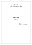
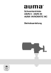
1. Introduction
Two Rotor Aero-dynamical System (TRAS) is a laboratory set-up designed for
control experiments. In certain aspects its behaviour resembles that of a helicopter. From
the control point of view it exemplifies a high order nonlinear MIMO system with
significant cross-couplings. The system is controlled from a PC. Therefore it is delivered
with hardware and software which can be easily mounted and installed in a laboratory. You
obtain the mechanical unit with power supply and interface to a PC and the dedicated
RT-DAC/PCI I/O board configured in the Xilinx technology. The software operates in
real-time under MS Windows XP/W7 using MATLAB R2009a/b, R2010a/b, R2011a/b
and R201a with RTW and RTWT toolboxes.
Control experiments are programmed and executed in real-time in the
MATLAB/Simulink environment. Thus it is strongly recommended to a user to be familiar
with the RTW and RTWT toolboxes. One has to know how to use the attached models and
how to create his own models.
The approach to control problems corresponding to the TRAS proposed in this
manual involves some theoretical knowledge of laws of physics and some heuristic
dependencies difficult to be expressed in analytical form.
DC-motor
tachogenerator
tail rotor
beam
counterbalance
DC-motor
tachogenerator
main rotor
power interface
RT-DAC4/PCI
board
articulation with
measurement
encoders
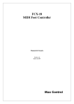
Fig. 1.1 The laboratory set-up: helicopter-like system
A schematic diagram of the laboratory set-up is shown in Fig. 1.1. The TRAS
consists of a beam pivoted on its base in such a way that it can rotate freely both in the
horizontal and vertical planes. At both ends of the beam there are rotors (the main and tail
rotors) driven by DC motors. A counterbalance arm with a weight at its end is fixed to the
beam at the pivot. The state of the beam is described by four process variables: horizontal
and vertical angles measured by position sensors fitted at the pivot, and two corresponding
angular velocities. Two additional state variables are the angular velocities of the rotors,
measured by tacho-generators coupled with the driving DC motors.
TRAS User’s Manual
-5-
In a casual helicopter the aerodynamic force is controlled by changing the angle of attack of
the rotors. The laboratory set-up from Fig. 1.1 is so constructed that the angle of attack is
fixed. The aerodynamic force is controlled by varying the speed of rotors. Therefore, the
control inputs are the supply voltages of the DC motors. A change in the voltage value
results in a change of the rotation speed of the propeller which results in a change of the
corresponding position of the beam. Significant cross-couplings are observed between the
actions of the rotors: each rotor influences both position angles. Designing of stabilising
controllers for such a system is based on decoupling. For a decoupled system an
independent control input can be applied for each coordinate of the system.
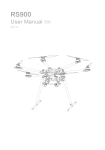
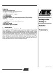
An IBM-PC compatible computer can be used for real-time control of TRAS. The
computer must be supplied with an interface board (RT-DAC/PCI). Fig. 1.2 shows details
of the hardware configuration of the control system for TRAS.
D/A
RT-DAC4/PCI
board
αv
ωh
ωv
Uh
αh
Uv
power interface
physical model
Fig. 1.2 Hardware configuration of TRAS
The control software for TRAS is included in the TRAS toolbox. This toolbox uses the
RTWT and RTW toolboxes from MATLAB.
TRAS Toolbox is a collection of M-functions, MDL-models and C-code MEX-files that
extends the MATLAB environment in order to solve TRAS modelling, design and control
problems. The integrated software supports all phases of a control system development:
• on-line process identification,
• control system modelling, design and simulation,
• real-time implementation of control algorithms.
TRAS Toolbox is intended to provide a user with a variety of software tools enabling:
• on-line information flow between the process and the MATLAB environment,
• real-time control experiments using demo algorithms,
• development, simulation and application of user-defined control algorithms.
TRAS User’s Manual
-6-
1.2
Hardware and software requirements.
TRAS Toolbox is distributed on a CD-ROM. It contains the software and TRAS User’s
Manual. The Installation Manual is distributed in a printed form.
Hardware
Hardware installation is described in the Installation manual. It consists of:
• TRAS Mechanical Unit,
• Power interface and wiring allowing electrical connections to the TRAS set-up,
• RT-DAC/PCI I/O board. The board contains FPGA equipped with dedicated logic
design,
• Pentium or AMD based personal computer.
Software
For development of the project and automatic building of the real-time program the
following software has to be properly installed on the PC:
• Microsoft Windows XP/W7,
• MATLAB version R2009a/b, R2010a/b, R2011ab or R2012a with appropriate
versions of Simulink RTW and RTWT toolboxes (not included),
• Control Toolbox from MathWorks Inc. to develop the project,
• The TRAS toolbox which includes specialised drivers for the TRAS System. These
drivers are responsible for communication between MATLAB and the
RT-DAC/PCI measuring and control board.
The built-in Open Watcom compiler is applied.
Manuals:
• Installation Manual
• User’s Manual
1.3
The experiments and corresponding to them measurements have been
conducted by the use of the standard INTECO system. Every new system
manufactured and developed by INTECO can be slightly different to those
standard devices. It explains why a user can obtain results maybe slightly
different to these given in the manual.
FEATURES of TRAS
•
•
•
•
A highly nonlinear MIMO system ideal for illustrating complex control algorithms.
The set-up is fully integrated with MATLAB/Simulink and operates in real-time
in MS Windows.
Real-time control algorithms can be rapidly prototyped. No C code programming is
required.
The software includes complete dynamic models.
TRAS User’s Manual
-7-
•
The User’s Manual, library of basic controllers and a number of pre-programmed
experiments familiarise the user with the system in a fast way.
Application note
The documentation assumes that the user has a basic experience with MATLAB, Simulink,
RTW and RTWT toolboxes from MathWorks Inc.
1.4
Software installation
Insert the installation CD and proceed step by step following displayed commands.
TRAS User’s Manual
-8-
2. TRAS Control Window
2.1
Starting and testing procedures
The TRAS system is an “open” type. It means that a user can design and solve any TRAS
control problem on the basis of the attached hardware and software. The software includes
device drivers compatible with RTWT toolbox. It is assumed that a user is familiarised
with MATLAB tools especially with RTWT toolbox. Therefore we do not include the
detailed description of this tool.
The user has a rapid access to all basic functions of the TRAS System from the TRAS
Control Window. It includes: identification, drivers, simulation model and application
examples.
In the Matlab command window type
tras
and then the TRAS Control Window opens (see Fig. 2.1)
Fig. 2.1 TRAS Control Window
TRAS Control Window contains: testing tools, drivers, models and demo applications. The
user has a rapid access to all basic functions of the TRAS control system from TRAS
Control Window.
TRAS Control Window shown in Fig. 2.1 contains four groups of the menu items:
TRAS User’s Manual
-9-
•
•
•
•
•
2.2
Tools
- Basic Test, Manual Setup, Reset Encoders and Stop Experiment,
Drivers
- RTWT Device Driver,
Simulation Models: Pitch , Azimuth and 2-DOF model,
Identification - Steady State Characteristics,
Demo Controllers – PID azimuth, PID pitch and cross-coupled PID controller.
Basic test
This section explains how to perform the tests. One can check if mechanical assembling
and wiring has been done correctly. The tests have to be performed obligatorily after
assembling the system. They are also necessary if an incorrect operation of the system
happens. Due to the tests sources of the system fails can be tracked. The tests have been
designed to validate the existence and sequence of measurements and controls. They do not
relate to accuracy of the signals.
At the beginning one has to be sure that all signals are transmitted and transferred in a
proper way. The following steps are applied:
•
Double click the Basic Tests button. The Basic Test window appears (Fig . 2.2)
Fig . 2.2 The Basic Tests window
The experiment may be stopped in any time. Double click on the Stop block in the TRAS
Control Window or somewhere else. If you wish to stop the visualisation process click once
on the Stop bar in the Simulation menu. As well the emergency switch can be used anyway.
The first step in the TRAS testing is to check if the RT-DAC/PCI measuring and control
board is installed properly.
TRAS User’s Manual
-10-
• Double click the Detect RT-DAC/PCI board button. One of the messages shown in
Fig. 2.3 opens. If the board has been correctly installed, the base address, and the
number of logic version of the board are displayed.
Fig. 2.3 Result of the step 1
If the board is not detected then check whether the board has been mounted correctly into a
slot of the computer. The boards are checked very precisely before sending to a customer.
In principle, a wrong assembling is the only reason of failure in detecting the board.
The next step consists in resetting the encoders. It means that the initial position of the
beam is stored in the interface board.
• Double click the Reset Angles button. When Fig. 2.4 opens, move the TRAS system
to the origin position and then click the Yes option. The encoders reset and zero
positions of the beam are going to be remembered.
Fig. 2.4 The Reset Angles window
•
Double click the Check Angles button. When the window opens click Yes, then,
move by hand the beam of TRAS in all directions and observe measurements on the
screen (see Fig. 2.5).
TRAS User’s Manual
-11-
Fig. 2.5 Measurements of the beam motion
In the next step one checks if the main and tail motors work properly.
• Double click the Open loop control button. When Fig. 2.6 opens one can to set the
control inputs to the main and tail motor. The vertical axis corresponds to the main
motor and the horizontal axis corresponds to the tail motor. When you locate the
mouse pointer at [0 0.5] and click, then the control equal to 0.5 is set for the main
motor. And if you click at [0.5 0] the control 0.5 is set for the tail motor. Using the
mouse, click and slowly drug a rectangle. The motors rotate with respect to the
mouse pointer location (the intersection of the green and red lines in Fig. 2.6). The
red ends of the blue lines show the rotational velocities of the propellers. If the
rectangle movement of the mouse is finished a picture similar to that given in Fig.
2.6 should be visible.
TRAS User’s Manual
-12-
Fig. 2.6 Motors control and checking of tacho-generators
Troubleshooting
Message or faulty action
Board not detected
Angles measurements failed
Propellers do not rotate
Velocities are not measured
2.3
Solution
Check mounting of the board. Check if the
driver is installed
Check the Enc socket and wiring
Check the M socket, Mains and ON switch
Check the T socket and wiring
TRAS Manual Setup
The TRAS Manual Setup program gives access to the basic parameters of the laboratory
Two Rotor Aerodynamical System setup. The most important data transferred from the
RT-DAC/PCI board and the measurements of the TRAS may be shown. Moreover, the
control signals may be set.
The application contains four frames (see Fig. 2.7):
• RT-DAC/PCI board,
• Encoders,
• Control and
• Tacho.
TRAS User’s Manual
-13-
Fig. 2.7 View of the TRAS Manual Setup window
All the data accessible from the TRAS Manual Setup program are updated 10 times per
second.
RT-DAC/PCI board frame
The RT-DAC/PCI board frame presents the main parameters of the PCI board.
No of detected boards
Reads the number of detected RT-DAC/PCI boards. If the number is equal to zero it means
that the software has not detected none of the RT-DAC/PCI board. When more then one
board is detected the Board list must be used to select the board that communicates with
the program.
2.3.1.1 Board
Contains the list applied to the selected board currently used by the program. The list
contains a single entry for each RT-DAC/PCI board installed in the computer. A new
selection at the list automatically changes values of the remaining parameters.
Bus number
Displays the number of the PCI bus where the current RT-DAC/PCI board is plugged-in. If
more then one board is used this parameter may be useful to distinguish the boards.
Slot number
The number of the PCI slot in which the current RT-DAC/PCI board is plugged-in. If more
then one board is used this parameter may be useful to distinguish the boards.
Base address
The base address of the current RT-DAC/PCI board. The RT-DAC/PCI board occupies 256
bytes of the I/O address space of the microprocessor. The base address is equal to the
beginning of the occupied I/O range. The I/O space is assigned to the board by the
computer operating system and may be different for various computers.
TRAS User’s Manual
-14-
The base address is given in the decimal and hexadecimal forms.
Logic version
The number of the configuration logic of the on-board FPGA chip. A logic version
corresponds to the configuration of the RT-DAC/PCI boards defined by this logic.
Application
The name of the application the board is dedicated for. The name contains four characters.
I/O driver status
The status of the driver that allows the access to the I/O address space of the
microprocessor. The status has to be OK string. In the other case the driver HAS TO BE
INSTALLED.
Encoders frame
The state of the encoder channels is given in the Encoder frame. The encoders are applied
to measure the azimuth and pitch angles.
Azimuth, Pitch
The values of the encoder counters, the angles expressed in radians and the encoder reset
flags are listed in the Azimuth and Pitch rows.
Value
The values of the encoder counters are given in the respective columns. The values are
16-bit integer numbers. When an encoder remains in the reset state the corresponding value
is equal to zero.
Angle [rad]
The angular positions of the encoders expressed in radians are given in the respective
columns. If the encoder remains in the reset state the corresponding angle is equal to zero.
Reset
When the checkbox is selected the corresponding encoder remains in the reset state. The
checkbox has to be unchecked to allow the encoder to count the position.
Control frame
The Control frame allows to change the control signals. DC drives are controlled by PWM
signals.
Azimuth and Pitch edit fields and sliders
The control edit boxes and the sliders are applied to set a new control values of the
corresponding DC drives. The control value may vary from –1.0 to 1.0.
STOP
The pushbutton is applied to switch off the control signals. If it is pressed then both the
azimuth and pitch control values are set to zero.
Azimuth and Pitch PWM prescaler
TRAS User’s Manual
-15-
The divider of the PWM reference signal is given. The frequency of the corresponding
PWM control is equal to:
FPWM = 40000/1023/(1+PWMPrescaler) [kHz]
Azimuth and Pitch Thermal flag / status
The thermal flags and the thermal statuses of the power amplifiers. If the thermal status
box is checked the corresponding power interface is overheated. If the power interface is
overheated and the corresponding thermal flag is set the RT-DAC/PCI board switches off
the PWM control signal corresponded to the overheated power amplifier.
Tacho frame
The Tacho frame displays two measured analog signals generated by the tachogenerators.
The voltages and the corresponding velocities of the propellers are displayed.
Azimuth and Pitch Voltage [V]
Displays the voltage at the outputs of the tacho generators.
Azimuth and Pitch Velocity [RPM]
Displays the velocity of the propellers. The velocities are calculated based on the
corresponding voltages and are given in RPM.
2.4
RTWT Device Driver
The driver is a software go-between for the real-time MATLAB environment and the
RT-DAC/PCI I/O board. The control and measurements are transferred. Click the TRAS
Device Driver button and the driver window opens (Fig. 2.8).
Fig. 2.8 RTWT Device Driver
When one wants to build his own application one can copy this driver to a new model.
TRAS User’s Manual
-16-
Do not do any changes inside the original driver. They can be introduced only
inside its copy!!! Make a copy of the installation CD.
The device driver has two inputs: control u (t ) ⊂ [− 1 + 1] and signal Reset. If the Reset
signal changes to one the encoders are reset and do not work. If the Reset signal is equal to
zero encoders work in the standard way. It means when switching occurs, encoders reset
and start measure when the switch returns to the zero (normal) position. It is important that
the Reset switch works only when the real-time code is executed.
The mask of this block (shown
Fig. 2.9) contains base address of
the
RT-DAC/PCI
board
(automatically detected with the
help
RTDACPCIBaseAddress
function) and the sampling period
which default value is set to 0.002
sec. If one wants to change the
default sampling time he must do
it in this mask also.
Fig. 2.9 Mask of the device driver
The details of the device driver are depicted in Fig. 2.10. The driver uses functions which
communicates directly with a logic stored at the RT-DAC/PCI board.
Parameters
Mux
3
Reset Encoder
TRAS_ResetEncoder
ResetEncoder
Measurements
1
ResetEncoderGain
0
TRAS_BitstreamVersion
Bitstream Version
(0
0)
TRAS_PWMPrescaler
PWMPrescalerSource
(1
1)
PWMPrescaler
TRAS_ThermFlag
ThermFlagSource
1
PWMPrescalerGain
1
ThermFlagGain
ThermFlag
1
TRAS_PWMTherm
Demux Azimuth Therm Status
Therm Status
1
Pitch Therm Status
Control
TRAS_Encoder
1
Azimuth PWM
Encoder
Mux
2
Azimult 0 PWM
TRAS_PWM
Saturation
PWM
1
-K-
1
Azimuth Angle
Demux
Encoder Convert to rad
1024 PPR
1
2
Pitch Angle
PWMGain
3
Azimuth RPM
TRAS_AnalogInput
Analog Input
-KConvert to RPM
Demux
4
Pitch RPM
Fig. 2.10 Interior of the RTWT device driver
TRAS User’s Manual
-17-
2.5
Simulation Models
There are three simulation models available for the TRAS system. The first one is a
1-DOF (degree of freedom) azimuth model. This model simulate behaviour of the system
in the horizontal plane only. Click the 1-DOF Azimuth Simulation Model button to open
the model shown in Fig. 2.11. Next, click the subsystem block to see details of the model.
TRAS
azimuth
model
rpm_a
ctrl_a
Step1
0
pos_am
Scope
RPM_A
1
ctrl_a
-K-
1
rpm_a
CTR_A
FORCE_A
1
s
-K-
x2
1
s
q
DCP-azimuth
x6
cos(u)
2
pos_am
0
x6=0
R_A2
|u|
-K-
-K-
Abs
Fig. 2.11 The Azimuth Simulation model and its interior
A 1-DOF pitch is the second model. It describes behaviour of the system in the vertical
plane. Click the 1-DOF Pitch Simulation Model button and click the subsystem block to
see the 1-DOF pitch model and its interior (see Fig. 2.12)
TRAS User’s Manual
-18-
TRAS
pitch
model
rpm_p
ctrl_p
Step1
0
pos_pm
rpm vel
pitch pos
Scope
0
y2
r
1
ctrl_p
x6
1
rpm_p
RPM_P
CTR_P
m7
-K-
FORCE_P
1
s
DCP_pith
-K-
1
s
2
pos_pm
-K|u|
-K-
-K-
Fig. 2.12 The Pitch Simulation model and its interior
The third one is the complete simulation model. It describes movements in both planes
with an interaction between the pitch and azimuth axes. Click the 2-DOF Simulation
Model button and the subsystem block to see the model and its interior (see Fig. 2.13)
TRAS
2_dof
model
rpm_a
azimuth rpm
ctr_a
0
pos_a
rpm_p
azimuth pos
pitch rpm
ctr_p
0
AZIMUTH
pos_p
pitch pos
PITCH
TRAS User’s Manual
-19-
DCP-azimuth
-K-
RPM_A
1
ctr_a
CTR_A
FORCE_A
-K-
1
s
x2
q
x6
1
rpm_a
1
s
2
pos_a
cos(u)
|u|
-K-K-
-K-
-K-
y2
r
x6
RPM_P
2
ctr_p
3
rpm_p
CTR_P
FORCE_P
1
s
-K-
-K-
1
s
4
pos_p
DCP_pith
|u|
-K-K-K-
Fig. 2.13 The 2-DOF simulation model and its interior
TRAS User’s Manual
-20-
3. Model and parameters
Modern methods of design and adaptation of real-time controllers require high quality
mathematical models of the system. For high order, nonlinear cross-coupled systems
classical modelling methods (based on Lagrange equations ) are often very complicated.
That is why a simpler approach is often used, which is based on block diagram
representation of the system which is very suitable for the SIMULINK environment. The
relations between the block diagram and mathematical model of the TRAS are explained in
sections 4.2 – 4.5.
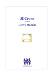
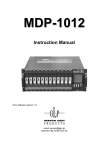
Fig. 3.1. shows an aero-dynamical system considered in this manual. At both ends
of a beam, joined to its base with an articulation, there are two propellers driven by DCmotors. The articulated joint allows the beam to rotate in such a way that its ends move on
spherical surfaces. There is a counter-weight fixed to the beam and it determines a stable
equilibrium position. The system is balanced in such a way, that when the motors are
switched off, the main rotor end of beam is lowered. The controls of the system are the
motor supply voltages.
The measured signals are: position of the beam in the space that is two position
angles and angular velocities of the rotors. Angular velocities of the beam are software
reconstructed by differentiating and filtering measured position angles of the beam.
tail rotor
main rotor
tail shield
main shield
DC-motor +
tacho
free-free beam
DC-motor +
tacho
articulation
Counter balance
Fig. 3.1. Aero-dynamical model of TRAS
The block diagram of the TRAS model is shown in Fig. 3.2. The control voltages U h and
U v are inputs to the DC-motors which drive the rotors (PWM mode).
A rotation of the propeller generates an angular momentum which, according to the law of
conservation of angular momentum, must be compensated by the remaining body of the
TRAS beam. This results in the interaction between two transfer functions, represented by
the moment of inertia of the motors with propellers khv and kvh (see Fig. 3.2). This
interaction directly influences the velocities of the beam in both planes. The forces Fh and
Fv multiplied by the arm lengths l h (α v ) and l v are equal to the torques acting on the arm.
TRAS User’s Manual
-21-
Gh(ω h, Ω h)
Fh
Uh
Ηh(Uh,t)
ωh
Fh(ωh)
Kh
Mh
lh(αv)
Ωh
1/Jh(α
α v)
1/s
DC-motor with
tail rotor
1/s
αh
fh
khv
kvh
DC-Motor with
main rotor
Uv
Ηv(Uv,t)
fv
ωv
αv
Fv(ωv)
Fv
1/Jv
1/s
lv
Mv
Gv(ω v, Ωv)
Ωv
Kv
1/s
Rh(αv, Ωh)
Fig. 3.2 Block diagram of the TRAS model
The following notation is used in Fig. 3.2:
α h is horizontal position (azimuth position) of TRAS beam [rad],
Ω h is angular velocity (azimuth velocity) of TRAS beam [rad/s],
U h is horizontal DC-motor PWM control input,
ω h is rotational speed of tail rotor [rad/s] - nonlinear function
ωh=H h(U h , t ) [rad/s],
Fh is aerodynamic force from tail rotor - nonlinear function
Fh=Fh(wh) [N],
l h is effective arm of aerodynamic force from tail rotor lh=lh(av) [m],
J h is nonlinear function of moment of inertia with respect to vertical axis,
Jh = Jh(av) [kg m2],
M h is horizontal turning torque [ Nm],
K h is horizontal angular momentum [Nms],
f h is oment of friction force in vertical axis [Nm],
α v is vertical position (pitch position) of TRAS beam [ rad],
Ωv is angular velocity (pitch velocity) of TRAS beam [rad/s],
U v is vertical DC-motor PWM voltage control input,
ω v is rotational speed of main rotor - nonlinear function ωv=H v(U v , t) [rad/s],
Fv is aerodynamic force from main rotor - nonlinear function Fv = Fv(ωv ) [N],
lv is arm of aerodynamic force from main rotor [m],
J v is moment of inertia with respect to horizontal axis [kg m2],
TRAS User’s Manual
-22-
M v is vertical turning moment [ Nm],
K v is vertical angular momentum [Nms],
f v is moment of friction force in horizontal axis [Nm],
Rv is vertical returning moment Rh = f cf + f g = Rh(αv ,Ωh ) [Nm],
J hv is vertical angular momentum from tail rotor [Nms],
J vh is horizontal angular momentum from main rotor [Nms],
H v is differential equation ω v = H v (U v , t ) ,
H h is differential equation ω h = H h (U h , t ) ,
Gv is aerodynamical damping torque from main rotor Gv (ω v , Ω v ) ,
Gh is aerodynamical damping torque from tail rotor
Gh (ω h , Ω h ) .
Controlling the system consists in stabilising the TRAS beam in an arbitrary (within
practical limits) desired position (pith and azimuth) or making it to track a desired
trajectory. Both goals may be achieved by means of appropriately chosen controllers. The
user can select between two types of PID controllers and a state feedback controller (see
section 6).
3.2
Nonlinear model
The mathematical model is developed with some simplifying assumptions. First, it
is assumed that the dynamics of the propeller subsystem can be described by the first order
differential equations. Further, it is assumed that friction in the system is of the viscous
type. It is assumed also that the propeller-air subsystem could be described in accord with
postulates of the flow theory.
The above assumptions allow us to define the problem clearly. First, consider the
rotation of the beam in the vertical plane i.e. around the horizontal axis. Having in mind
that the driving torques are produced by the propellers the rotation can be described in
principle as the motion of a pendulum. From the second dynamics law of Newton we
obtain:
d 2α v
M v = Jv
(1)
dt 2
where: M v
- total moment of forces in the vertical plane,
Jv
- the sum of moments of inertia relative to the horizontal axis,
αv
- the pitch angle of the beam.
Then:
6
M v = ∑ M vi ,
i =1
8
J v = ∑ J vi
i =1
To determine the moments of forces applied to the beam and making it rotate
around the horizontal axis consider the situation shown in Fig. 3.3 .
TRAS User’s Manual
-23-
horizontal axis
of rotation
lt
mtrg
m tg l
cb
lm
−αv
lb
m bg
mmg
mmrg
mcbg
Fig. 3.3 Gravity forces in TRAS corresponding to the
return torque which determines the equilibrium
position of the system.
 m

 m
 
m

M v1 = g  t + mtr + mts lt −  m + mmr + mms lm  cos αv −  b lb + mcd lcb  sin αv 
  2
 
 2

 2

M v1 = g [( A-B ) cos αv − C sin αv ]
where:
m

A =  t + mtr + mts  lt
 2

m

B =  m + mmr + mms  lm
 2

m

C =  b lb + mcd lcb 
 2

where: M v1 is the return torque corresponding to the forces of gravity,
mmr is the mass of the main DC-motor with main rotor,
mm is the mass of the main part of the beam,
mtr is the mass of the tail motor with tail rotor,
mt is the mass of the tail part of the beam,
mcb is the mass of the counter-weight,
mb is the mass of the counter-weight beam,
mms is the mass of the main shield,
mts is the mass of the tail shield,
lm is the length of the main part of the beam,
lt is the length of the tail part of the beam,
TRAS User’s Manual
-24-
lb is the length of the counter-weight beam,
lcb is the distance between the counter-weight and the joint.
g is the gravitational acceleration,
vertical axis of rotation
horizontal axis of rotation
−αv
thrust of main
rotor
Fv (ωm)
Mv4+ Mv2
Main rotor
Fig. 3.4 Propulsive force moment and friction moment in TRAS
M v 2 = l m Fv (ωm )
M v 2 is the moment of the propulsive force produced by the main rotor,
ω v is angular velocity of the main rotor,
Fv (ωv ) denotes the dependence of the propulsive force on the angular velocity of
the rotor. It should be measured experimentally (see section 4.5).
 m
m 

m

M v 3 = − Ωh2  m + mmr + mms  l m +  t + mtr + mts  lt + mcb lcb + b lb  sin αv cos αv
2 

 2

 2
or in the compact form:
M v 3 = − Ωh2 ( A+B+C ) sin αv cos αv
M v 3 - is the moment of centrifugal forces corresponding to the motion of the beam around
the vertical axis,
dα h
(2)
dt
Ωh - is the angular velocity of the beam around the vertical axis, α h - is the azimuth angle
of the beam.
and: Ωh =
M v 4 = − Ωv f v
TRAS User’s Manual
-25-
M v 4 is the moment of friction depending on the angular velocity of the beam around the
horizontal axis.
dα v
dt
Ωv is the angular velocity around the horizontal axis,
where: Ωv =
(3)
f v is a constant,
M v 5 is the cross moment from U h , M v 5 = U h k hv ,
k hv is constant,
M v 6 is the damping torque from rotating propeller M v 6 = − a1Ωv abs(ωv ) ,
a1 is constant.
According to Fig. 3.4 we can determine components of the moment of inertia
relative to the horizontal axis. Notice that this moment is independent of the position of
the beam.
J v1 = mmr l m2 ,
J v4
J v7
l m2
, J v 3 = mcb lcb2
3
lt2
2
= mtr lt , J v 6 = mt
3
J v 2 = mm
lb2
= mb , J v 5
3
mms 2
=
rms + mms l m2 ,
2
J v 8 = mts rts2 + mts lt2
rms is the radius of the main shield,
rts is the radius of the tail shield.
Similarly we can describe the motion of the beam around the vertical axis. Having
in mind that the driving torques are produced by the rotors and that the moment of inertia
depends on the pitch angle of the beam the horizontal motion of the beam (around the
vertical axis) can be described in principle as rotative motion of a solid:
Mh = Jh
d 2 αh
dt 2
(4)
where: M h is the sum of moments of forces acting in the horizontal plane,
J h is the sum of moments of inertia relative to the vertical axis.
4
Then: M h = ∑ M hi ,
i =1
8
J h = ∑ J hi
i =1
To determine the moments of forces applied to the beam and making it rotate
around the vertical axis consider the situation shown in Fig. 3.5.
TRAS User’s Manual
-26-
thrust of tail rotor
Fh(ωt)
vertical axis of rotation
αh
lt
lm
Mh1
Fig. 3.5 Moments of forces in horizontal plane (as seen from above)
M h1 = lt Fh(ω t ) cos α v
ω t is angular velocity of tail rotor, Fh (ωt ) - denotes the dependence of the
propulsive force on the angular velocity of the tail rotor (should be determine
experimentally, see section 4.5)
M h 2 = − Ωh f h
M h 2 is the moment of friction depending on the angular velocity of the beam
around the vertical axis,
f h is constant,
M h3 is the cross moment from U v , M h3 = U v k vh ,
k vh is constant,
M h 4 is the damping torque from rotating propeller, M h 4 = − a 2 Ωh abs(ωh ) ,
a2 is constant.
According to Fig. 3.5. we can determine components of the moment of inertia
relative to vertical axis (it depends on pitch position of the beam).
mm 
2
 l cos α  ,
v
 m
3
mb 
2
 l sin α  ,
=
v
 b
3
2
= mmr  l m cos αv  ,
mt 
2
 l cos α  ,
v
 t
3
J h1 =
J h2 =
J h3
J h 4 = mtr  lt cos αv  ,
J h5
J h7 =
2
J h 6 = mcb  lcb sin αv 
2
mts 2
2
2
rts + mts  lt cos αv  , J h8 = mms rms2 + mms  l m cos αv 
2
or in the compact form:
J h = E cos 2 αv + D sin 2 αv + F
TRAS User’s Manual
-27-
where: D,E,F are constants:
mb 2
lb + mcb lcb2 ,
3
m

m

E =  m + mmr + mms  l m2 +  t + mtr + mts  lt2 ,
 3

 3

m
F = mms rms2 + ts rts2
2
D=
M v1 = g {( A-B ) cos αv − C sin αv }
Using (1)-(4) we can write the equations describing the motion of the system as follows:
dΩv l m Fv(ωm ) − Ωv k v + g (( A − B ) cos αv − C sin αv )
=
....
dt
Jv
1
− Ωh2 ( A + B + C )sin 2αvU h k hv + U h k hv − a1Ωv abs(ωv )
... 2
Jv
(5)
dαv
= Ωv ,
dt
(6)
lt Fh(ωt ) cos αv − Ωh k h + U v k vh − a 2 Ωh abs(ωh )
D sin 2 αv + E cos 2 αv + F
dK h M h
=
dt
Jh
=
dα h
= Ωh ,
dt
Ωh =
Kh
J h (αv )
(7)
(8)
and two equations describing the motion of rotors:
Ih
dωh
dωv
= U h − H h-1 (ωh ) and I v
= U v − H v-1 (ωv )
dt
dt
I h is moment of inertia of the tail rotor,
I v is moment of inertia of the main rotor.
The above model of the motor-propeller dynamics is obtained by substituting the nonlinear
system by a serial connection of a linear dynamic system and static nonlinearity.
TRAS User’s Manual
-28-
3.3
State equations
Finally, the mathematical model of TRAS (compare Fig. 3.2) becomes the set of
four nonlinear differential equations with two linear differential equations and four
nonlinear functions.
Ω h 
K h 
α 
α 
 h
 h
u h 
ω 
ω 
U=  is the input, X =  h  is the state, and Y =  t  is the output vector.
u v 
Ω v 
K v 
α v 
α v 
ω 
ω 
 v
 v
In order to apply the model for control of TRAS the parameters and nonlinear functions
should be determined first. They can be divided into three groups:
• physical parameters,
• nonlinear static characteristics,
• time constants of the linear part of the model.
They are described in details in the next section.
3.4
Physical parameters
To obtain the values of model coefficients it is necessary to perform some
measurements. First, geometrical dimensions and moving masses of TRAS should be
measured. There are the following results of measurements for a given laboratory TRAS
set-up.
mtr = 0.225 [kg]
lt = 0.216
lm = 0.202
lb = 0.145
lcb = 0.15
rms = 0.145
rts = 0.10
mmr = 0.252 [kg]
[m]
[m]
[m]
[m]
[m]
[m]
[m]
mcb = 0.0256 [kg]
mt = 0.032 [kg]
mm = 0.03 [kg]
mb = 0.01 [kg]
mts = 0.061 [kg]
mms = 0.083 [kg]
Using the above measurements the moment of inertia about the horizontal axis can be
calculated as:
8
J v = ∑ J iv = 0.0307 [kg m 2 ] .
i
The terms of the sum are calculated from elementary physics laws:
TRAS User’s Manual
-29-
J v1 = mmr l m2
= 0.0103 [kg m 2 ]
J v 2 = mm l m2 / 3 = 0.00040 [kg m 2 ]
J v 3 = mcb l cb2
= 0.00057 [kg m 2 ]
J v 4 = mb l b2 / 3
J v 5 = mtr l t2
= 0.0007 [kg m 2 ]
= 0.0105 [kg m 2 ]
J v 6 = mt l t2 / 3 = 0.00049 [kg m 2 ]
J v 7 = mms (rms2 / 2 + l m2 ) = 0.0043 [kg m 2 ]
J v 8 = mts (rts2 / 2 + l t2 )
= 0.0035 [kg m 2 ]
The calculated moment of inertia about the vertical axis is:
8
J h = ∑ J hi ,
i
where the terms of the sum are:
J h1 = mt (lt cos αv ) / 3
= 0.00049 cos 2 αv
[kg m 2 ]
J h 2 = mm (lm cos αv ) / 3
= 0.0004 cos 2 αv
[kg m 2 ]
J h3 = mb (lb sin av ) / 3
= 0.0007 sin 2 αv
[kg m 2 ]
= 0.0103 cos 2 αv
[kg m 2 ]
= 0.0105 cos 2 αv
[kg m 2 ]
2
2
2
J h 4 = mmr (lm cos αv )
2
J h5 = mtr (lt cos αv )
2
J h 6 = mcb (lcb sin αv )
2
(
(r
= 0.00057
J h 7 = mts rts2 / 2 + lt2 cos 2 αv
J h8 = mms
2
ms
)
)
sin 2 αv
= 0.0003 + 0.0028 cos 2 αv
/ 2 + lm2 cos 2 αv = 0.00087 + 0.0034 cos 2 αv
[kg m 2 ]
[kg m 2 ]
[kg m 2 ]
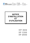
giving finally (Fig. 3.6):
9
J h = ∑ J hi = E cos 2 αv + D sin 2 αv+ F = 0.0279 cos 2 αv + 0.0013 sin 2 αv+ 0.0021 .
i
TRAS User’s Manual
-30-
moment of inertia Jh [kg m2]
0.03
0.025
0.02
0.015
0.01
0.005
0
-1.5
-1
-0.5
0
0.5
vertical position [rad]
1
1.5
Fig. 3.6 Moment of inertia J h
The returning torque from gravity forces is expressed by
8
M r = ∑ M ri ,
i
and its components are given by:
M r1 = - 9.81 mmlm cos αv / 2 = -0.0297 cos αv [N m]
M r 2 = - 9.81 mmr lm cos αv
= -0.4994 cos αv [N m]
M r 3 = - 9.81 mmslm cos αv
= -0.1645
cos αv [N m]
M r 4 = + 9.81 mt lt cos αv / 2 = 0.0339
cos αv [N m]
M r 5 = + 9.81 mtr lt cos αv
= 0.4768
cos αv [N m]
M r 6 = + 9.81 mtslt cos αv
= 0.1293 cos αv [N m]
M r 7 = - 9.81 mblb sin αv / 2
= 0.0711 sin αv [N m]
M r 8 = - 9.81 mcblcb sin αv
= 0.0377 sin αv [N m]
giving finally (Fig. 3.7)
8
M r = ∑ M ri = ( -0.0536 cos αv + 0.1088 sin αv ) [N m] .
i
TRAS User’s Manual
-31-
returning moment of gravity forces [Nm]
0.15
0.1
0.05
equilibrum point
0
-0.05
-0.1
-0.15
-0.2
-1.5
-1
-0.5
0
0.5
vertical position [rad]
1
1.5
Fig. 3.7 Returning moment of the gravity forces M r
The moment of the centrifugal forces is:
6
M cf = ∑ M cfi ,
i
where
M cf 1 = (mtr+mts )lt2 Ωh2 cos αv sin αv
=0.0133 Ωh2 cos αv sin αv [N m]
M cf 2 = mt lt2 Ωh2 cos αv sin αv / 4
= 0.00037 Ωh2 cos αv sin αv [N m]
M cf 3 = mblb2 Ωh2 cos αv sin αv / 4
=0.00052 Ωh2 cos αv sin αv
M cf 4 = mcblcb2 Ωh2 cos αv sin αv
=0.00057 Ωh2 cos αv sin αv [N m]
M cf 5 = mmlm2 Ωh2 cos αv sin αv / 4
=0.0003 Ωh2 cos αv sin αv [N m]
[N m]
M cf 6 = (mmr+mms )lm2 Ωh2 cos αv sin αv =0.0137 Ωh2 cos αv sin αv [N m]
giving finally (Fig. 3.8)
6
M cf = ∑ M cfi = 0.02876 Ωh2 cos αv sin αv [N m] .
i
TRAS User’s Manual
-32-
Fig. 3.8 Centrifugal returning torque
3.5
Static characteristics
It is necessary to identify the following functions:
• Two nonlinear input characteristics determining dependence of the DC-motor rotational
speed versus the input voltage (RPM characteristics): ωv = H v(U v ) and ωh = H h(U h )
To measure the characteristics double click the Static characteristics button in TRAS
Control Window. The window given in Fig. 3. opens. In this window one defines the
minimal and maximal control values and a number of measured points. The control order
can be set as: Ascending, Descending or Reverse. Also one can choose the pitch or azimuth
static characteristic. Note, that the control signal is normalised and changes in the range
[-1, +1] what corresponds to the input voltage range [-24V, +24V].
TRAS User’s Manual
-33-
Fig. 3.How to collect the points of the static characteristic
Block the beam before the experiment is started. Choose Azimuth axis (tail rotor) and click
the Run button. The constant value of the control activates the DC motor so long as a
steady state of the shaft angular velocity is achieved. Then, the velocity is measured and the
control value is changed to the next constant value and DC motor is activated again. These
steps are repeated to the end of the control range. Simultaneously, the measurements are
displayed in the screen. This action should be repeated for pitch axis (main rotor) to
obtained the both characteristics. Examples of the measured static characteristic for the
main and tail rotors are shown in Fig. 3.9.
rpm vs. PWM
8000
6000
rotor velocity [rpm]
4000
2000
0
-2000
-4000
-6000
-8000
-1
-0.8
-0.6
-0.4
-0.2
0
0.2
PWM control value [--]
0.4
0.6
0.8
1
Fig. 3.9 Main and tail rotor static characteristics
TRAS User’s Manual
-34-
If the characteristic is measured in Reverse mode (the control has been changed from –1 to
+1 and reverse), there are two slightly different plots.
• Two nonlinear characteristics determining dependence of the propeller thrust on DC
motor rotational speed (thrust characteristics): Fh=Fh(ω h ) , Fv =Fv(ωv ) .
The thrust static characteristics of the propellers should be measured in the case when the
propellers were changed by a user. In this case a proper electronic balance (not delivered
with the system) is necessary to measure the force created by rotational movements of the
propellers. The characteristics included in TRAS Toolbox and shown in this section has
been obtained by the manufacturer of TRAS.
3.5.1
Main rotor thrust characteristics
string
balance
weight
electronic
balance
Fig. 3.10 Measuring of the main rotor thrust characteristics
To perform measurements correctly block the beam so that it could not rotate
around the vertical axis, place the electronic balance under the beam in such a way that it
is pulled by the propeller straight up. To balance the beam in the horizontal position
attach a weight to the beam (as in Fig. 3.10) .
Fig. 3.11 Measured static thrust characteristics of the main rotor
TRAS User’s Manual
-35-
For further applications the measured characteristics should be replaced by their
polynomial approximations. For this purposes one can use the MATLAB polyfit.m
function. An example is given in Fig.3.6. The obtained polynomials have the form:
~
Fv = - 1.8 ⋅ 10 -18 ω v5 - 7.8 ⋅ 10 -16 ω v4 + 4.1 ⋅ 10 -11 ω v3 + 2.7 ⋅ 10 -8 ω v2 + 3.5 ⋅ 10 -5 ω v - 0.014
ω~v = - 5.2 ⋅ 10 3 U v7 - 1.1 ⋅ 10 2 U v6 + 1.1 ⋅ 10 4 U v5 + 1.3 ⋅ 10 2 U v4 - 9.2 ⋅ 10 3 U v3 - 31U v2 + 6.1 ⋅ 10 3 U v - 4.5
Fig. 3.12 Polynomial approximation of the main rotor characteristics
3.5.2
Tail rotor thrust characteristics
Fig. 3.13 shows laboratory set-up for measuring thrust of the tail rotor.
rope
balance
weight
electronic
balance
Fig. 3.13 Laboratory set-up for the tail rotor thrust characteristics
To measure the static thrust characteristics one should to rearrange the laboratory set-up as
shown in Fig. 3.13 and the electronic balance should be used.
The measured by the manufacturer of TRAS thrust static characteristics of the tail motor
are given in Fig. 3.14.
TRAS User’s Manual
-36-
Fig. 3.14 Thrust characteristics measured for the tail rotor.
For further applications the characteristics can be replaced by their polynomial
approximations. For this purposes one can use the MATLAB polyfit.m function. The
obtained polynomials are as follows:
~
Fh = - 2.6 ⋅ 10 - 20 ωh5 + 4.1 ⋅ 10 -17 ωh4 + 3.2 ⋅ 10 -12 ωh3 - 7.3 ⋅ 10 -9 ωh2 + 2.1 ⋅ 10 - 5 ωv + 0.0091
~ = 2.2 ⋅ 10 3 U 5 - 1.7 ⋅ 10 2 U 4 - 4.5 ⋅ 10 3 U 3 + 3 ⋅ 10 2 U 2 + 9.8 ⋅ 10 3 U - 9.2
ω
h
h
v
v
v
v
Fig. 3.15 Polynomial approximation of tail rotor characteristics
TRAS User’s Manual
-37-
4. RTWT model
In this section the process of building your own control system is described. The Realtime Windows Target (RTWT) toolbox is used. An example how to use the TRAS software
is shown later in section 5.3. In this section we give indications how to proceed in the
RTWT environment.
Before start, test your MATLAB configuration by building and running an
example of a real-time application. Real-time Windows Target Toolbox includes
the rtvdp.mdl model. Running this model will test the installation of the RealTime Workshop, Real-Time Windows Target toolboxes and the Real-Time
Windows Target kernel.
In the MATLAB window, type
rtvdp
Next, build and run the real-time model.
To build the system that operates in the real-time mode the user has to:
• create a Simulink model of the control system which consists of TRAS Device
Driver and other blocks chosen from the Simulink library,
• build the executable file under RTWT,
• start the real-time code from the Simulation/Start real-time code pull-down menu. In
this way the system runs in real-time.
4.2
Creating a model
The simplest way to create a Simulink model of the control system is to use one of the
models included in the Tras Control Window as a template. For example, click on the PID
Azimuth button and save it as MySystem.mdl name. The MySystem Simulink model is
shown in Fig. 4.1.
TRAS User’s Manual
-38-
Fig. 4.1 The MySystem Simulink model
Now, you can modify the model. You have absolute freedom to develop your own
controller. Remember to leave the TRAS device driver block in the window. This is
necessary to work in RTWT environment.
Though it is not obligatory, we recommend you to leave the scope. You need a scope to
watch how the system runs. The saturation blocks are built in the Tras driver block. They
limit the currents to the DC motors for safety reasons. However they are not visible for the
user who may amaze at the saturation of controls. Other blocks remaining in the window
are not necessary for our new project.
Creating your own model on the basis of an old example ensures that all internal options of
the model are set properly. These options are required to proceed with compiling and
linking in a proper way. To put the Tras Device Driver into the real-time code a special
make-file is required. This file is included to the TRAS software.
You can apply most of the blocks from the Simulink library. However, some of them
cannot be used (see RTW or RTWT references manual).
The scope block properties are important for an appropriate data acquisition and watching
how the system runs.
The Scope block properties are defined in the Scope property window (see Fig. 4.2). This
window opens after the selection of the Scope/Properties tab. You can gather measurement
data to the Matlab Workspace marking the Save data to workspace checkbox. The data is
placed under Variable name. The variable format can be set as structure or matrix. The
default Sampling Decimation parameter value is set to 1. This means that each measured
point is plotted and saved. Often we select the Decimation parameter value equal to 5 or
10. This is a good choice to get enough points to describe the signal behaviour and to save
the computer memory.
TRAS User’s Manual
-39-
Fig. 4.2 Setting the parameters of the Scope block
When the Simulink model is ready, click the Tools/External Mode Control Panel option
and next click the Signal Triggering button. The window presented in Fig. 4.3 opens.
Select Select All check button, set Source as manual, set Duration equal to the number of
samples you intend to collect, and close the window.
Fig. 4.3 The External Signal & Triggering window
4.3
Code generation and the build process
Once a model of the system has been created the code for the real-time mode can be
generated, compiled, linked and downloaded into the target processor.
TRAS User’s Manual
-40-
The code is generated by the use of Target Language Compiler (TLC) (see description of
the Simulink Target Language). The makefile is used to build and download object files to
the target hardware automatically.
First, you have to specify the simulation parameters of your Simulink model in the
Simulation parameters dialog box (Fig. 4.4). The Real-Time Workshop and Solver tabs
contain critical parameters.
Fig. 4.4 Solver tab
The Solver tab allows you to set the simulation parameters. Several parameters and options
are available in the window. The Fixed-step size editable text box is set to 0.01 (this is the
sampling period in seconds).
The Start time has to be set to 0 (Fig. 4.4). The solver method has to be selected. In our
example the fifth-order integration method − ode5 is chosen. The Stop time field defines
the length of the experiment. This value may be set to a large number. Each experiment can
be terminated by pressing the Stop real-time code button.
The Fixed-step solver is obligatory for real-time applications. If you use an
arbitrary block from the discrete Simulink library or a block from the drivers’
library remember, that different sampling periods must have a common
divider.
Third party compiler is not requested. The built-in Open Watcom compiler is used to create
real-time executable code for RTWT.
The RTW tag is shown in Fig. 4.5. The system target file name is rtwin.tlc. It manages the
code generation process. Notice, that rtwin.tmf template makefile is used. This file is
default one for RTWT building process.
TRAS User’s Manual
-41-
Fig. 4.5 Configuration parameters/Real-Time Workshop tab
If all the parameters are set properly you can start the real-time executable building
process. For this purpose press the Build push button at the Real Time Workshop tag (Fig.
4.5), or simply “CRTL + B”. Successful compilation and linking processes generate the
following message:
Model MyModel.rtd successfully created
### Successful completion of Real-Time Workshop build procedure for model: MyModel
Otherwise, an error message is displayed in the MATLAB Command Window.
In this case check again your MATLAB configuration and simulation parameters.
TRAS User’s Manual
-42-
5. Controllers and real-time experiments
In the following section we propose three PID controllers. It is possible to tune the
parameters of the controllers without analytical design. Such approach to the control
problem seems to be reasonable if a well identified model of TRAS is not available. The
effectiveness of the PID controllers discussed here is illustrated by control experiments.
PID controllers
One degree of freedom (1-DOF) control problem is the following. Design a controller that
will stabilise the system, or make it follow a desired trajectory in one plane (one degree of
freedom) while motion in the other plane is blocked mechanically or being controlled by
another controller.
If TRAS is free to move in both axes we refer to the control as two degree of freedom (2DOF). The four PID controllers for TRAS: PIDvv, PIDvh, PIDhv and PIDhh (h-horizontal
(azimuth), v-vertical (pitch)) are considered. The subscripts indicates the source-sink
relation for the controller. Each control signal (Uv and Uh) is the sum of two controller
outputs. For example, vertical control denoted later as Uv is the sum of two output signals:
PIDvv and PIDhv. The internal structure of each PID controller is shown in Fig. 5.15b.
There are three parameters to be set for every controller: KP, Ki and Kd. The TRAS control
in the vertical and horizontal planes requires setting altogether 12 (3×4) controller
parameters. Saturation blocks introduce four additional Isat parameters: Ivvsat, Ivhsat, Ihhsat and
Ihvsat, which are the limits of absolute values of the integrals of errors, and two: Uhmax and
Uvmax parameters, which are the limits of absolute value of controls. These 18 (12+4+2)
parameters have their default values.
5.2
1-DOF controllers
The task of the one-degree-of-freedom (1-DOF) controllers is to move TRAS to an
arbitrary position in the selected plane and to stabilise it there.
5.2.1
Vertical 1-DOF control
At the beginning we restrict our control objective to stabilising the system in the vertical
plane only. We reduce the original system to the 1-DOF system by mechanically fixing
(using the included clamp) its freedom to move in the horizontal plane. A corresponding
block diagram of the PID control system is shown in Fig. 5.1.
αvd
εv
Uv
PIDvv
1-DOF
SYSTEM
αv
αvd - desired pitch
Fig. 5.1 1-DOF pitch control system
TRAS User’s Manual
-43-
The block diagram below shows the system in a more detailed form (Fig. 5.2). Notice, that
only the vertical part of the control system is considered.
Gh(ω h, Ω h)
Fh
Uh
Ηh(Uh,t)
ωh
lh(αv)
Fh(ωh)
Kh
Mh
1/Jh(α
αv)
1/s
DC-motor with
tail rotor
Ωh
1/s
αh
fh
khv
kvh
DC-Motor with
main rotor
Uv
Ηv(Uv,t)
fv
ωv
αv
Fv(ωv)
Fv
1/Jv
1/s
lv
Mv
Gv(ω v, Ωv)
Kv
Ωv
1/s
Rh(αv, Ωh)
Fig. 5.2 The block diagram 1-DOF system (vertical plane)
5.2.2
Real-time 1-DOF pitch control experiment
Fix TRAS in the horizontal plane using the special plastic clamps delivered with TRAS.
Set it in the neutral vertical position and wait until the all oscillations are damped. In Tras
Control Window double click the Reset Encoders block.
Click the PID Pitch controller button and the model shown in Fig. 5.3 opens. Set all PID
controller coefficients as: K p = 0.6784 K i = 0.4415 and K d = 1.31196 . Also set saturation
of the integral part of the controller to 1.43. Build the model and click on the
Simulation/Connect to target option and Start real-time code option.
TRAS User’s Manual
-44-
TRAS 1-DOF PID Pitch
num(z)
den(z)
Control FIlter
Filtered
Control
Angle & Reference
Angle & Control
Azimuth Angle
0
Zero Azimuth
Control
Pitch Angle
PID
Reference Angle
Generator
Control
PID Controller
Azimuth RPM
0.3
Pitch Offset
Pitch RPM
Reset
1
TRAS
RPM
0
Normal
Reset
Encoders
Fig. 5.3 Real-time model for the pitch control
The results of the experiment are shown in Fig. 5.4. Notice, that control changes with high
frequency. This phenomena appears due to the quantization effects of the signal caused by
the differential part of the controller. For this reason the control signal is filtered to
obtaining an average value of the control signal. It is shown in the upper part of Fig. 5.4.
Fig. 5.4 Results of the PID pitch control
TRAS User’s Manual
-45-
The details of the above experiment are shown in Fig. 5.5, Fig. 5.6 and Fig. 5.7.
PID controller for pitch position - Filtered control
0.8
0.7
0.6
0.5
0.4
0.3
0.2
0.1
0
0
10
20
30
40
50
time [s]
60
70
80
90
80
90
Fig. 5.5 The filtered control
PID controller for pitch position - control
1
0.9
0.8
0.7
0.6
0.5
0.4
0.3
0.2
0
10
20
30
40
50
time [s]
60
70
Fig. 5.6 The non filtered control
TRAS User’s Manual
-46-
Pitch position and reference signal
0.3
0.2
0.1
0
-0.1
-0.2
-0.3
-0.4
-0.5
0
10
20
30
40
50
time [s]
60
70
80
90
Fig. 5.7 Pitch position and the reference signal
5.2.3
Horizontal 1-DOF control
In the next experiment we apply stabilising PID controller in the horizontal plane.
We block the system in one axis so that it cannot move in the vertical plane (using the
included fixing rectangle).. A corresponding block diagram of the control system is shown
in Fig. 5.8, and in a more detailed form in Fig. 5.9.
α hd
εh
PIDh
Uh
1-DOF
SYSTEM
αh
α hd -desired azimuth
Fig. 5.8 1-DOF control closed-loop system (azimuth stabilisation)
Notice that only the ‘horizontal’ part of the control system is considered.
TRAS User’s Manual
-47-
Gh(ω h, Ω h)
Fh
Uh
Ηh(Uh,t)
lh(αv)
Fh(ωh)
ωh
Kh
Mh
Ωh
1/Jh(α
αv)
1/s
DC-motor with
tail rotor
1/s
αh
fh
khv
kvh
DC-Motor with
main rotor
Uv
Ηv(Uv,t)
fv
ωv
αv
Fv(ωv)
1/Jv
1/s
lv
Mv
Fv
Ωv
Kv
1/s
Rh(αv, Ωh)
Gv(ω v, Ωv)
Fig. 5.9 The block diagram of 1-DOF system (horizontal plane)
5.2.4
Real-time 1-DOF azimuth control experiment
Fix TRAS in the vertical plane using the special fixing rectangle delivered with TRAS. Set
it in the zero position and click on the Reset Encoders block in Tras Control Window.
Click PID Azimuth controller and the model shown in Fig. 5.10 opens. Set all PID
controller coefficients as K p = 4.9395 K i = 0.0022 and K d = 5.1898 . Also set saturation
of the integral part of the controller to 1.0. Build the model and click on the
Simulation/Connect to target and Start real-time code options.
num(z)
TRAS 1-DOF PID Azimuth
den(z)
Filtered
Control FIlter
Control
Angle & Reference
Angle & Control
PID
Reference Angle
Generator
Azimuth Angle
Control
PID Controller
Pitch Angle
0
Zero Pitch Control
Azimuth RPM
Reset
RPM
1
0
Pitch RPM
Reset
Encoders
Normal
TRAS
Fig. 5.10 Real-time model for the PID azimuth control
TRAS User’s Manual
-48-
The results of the experiment are shown in Fig. 5.11. Notice a high frequency of the control
similar to that in the case of the pitch control. This phenomena appears due to the
quantization effects of the signal caused by the differential part of the controller. For this
reason the control signal is filtered. It is shown in the upper part of Fig. 5.11.
Fig. 5.11 Results of the PID azimuth control
The details of the above experiment are shown in Fig. 5.12, Fig. 5.13and Fig. 5.14.
PID controller for azimuth position - Filtered control
0.6
0.4
0.2
0
-0.2
-0.4
-0.6
-0.8
0
5
10
15
tim e [s]
20
25
30
Fig. 5.12 The filtered control
TRAS User’s Manual
-49-
P ID c ontroller for az im uth pos ition - c ontrol
0.5
0.4
0.3
0.2
0.1
0
-0.1
-0.2
-0.3
-0.4
-0.5
0
5
10
15
tim e [s ]
20
25
30
Fig. 5.13 The non filtered control
Azimuth position and reference signal
0.5
0
-0.5
0
5
10
15
time [s]
20
25
30
Fig. 5.14 The azimuth position and reference signal
TRAS User’s Manual
-50-
5.3
2-DOF PID controller
The structure of the cross-coupled multivariable PID controller is shown in Fig. 5.15.
a)
PIDhh
εh
Uh
PIDhv
PIDvh
εv
Uv
PIDvv
b)
Kp
ε
U
SKd
saturation block
U max
Ki/S
saturation block I sat
Fig. 5.15 Structure of the cross-coupled PID controller
a) general b) single PID block
The controller is described by the equations given bellow.
ε v = α vd − α v ,
ε h = α hd − α h ,
where: ε v , ε h are errors of the vertical (pitch) and horizontal angle (azimuth), α vd , α hd are
the reference values of the vertical and horizontal angles, α v , α h are the vertical and
horizontal angles.
The integrators are described by the following equations:
t
I vv (t ) = Kivv ∫ ε v dt ,
for − I vvsat ≤ I vv ≤ I vvsat
0
if ( I vv > I vvsat ) then I vv = I vvsat , if ( I vv < − I vvsat ) then I vv = − I vvsat ,
t
I vh (t ) = Kivh ∫ ε v dt ,
for − I vhsat ≤ I vh ≤ I vhsat
0
if ( I vh > I vhsat ) then I vh = I vhsat , if ( I vh < − I vhsat ) then I vh = − I vhsat ,
t
I hv (t ) = Kihv ∫ ε h dt ,
for − I hvsat ≤ I hv ≤ I hvsat
0
TRAS User’s Manual
-51-
if ( I hv > I hvsat ) then I hv = I hvsat , if ( I hv < − I hvsat ) then I hv = − I hvsat ,
t
I hh (t ) = Kihh ∫ ε h dt ,
for − I hhsat ≤ I hh ≤ Ihhsat
0
if ( I hh > I hhsat ) then I hh = I hhsat , if ( I hh < − I hhsat ) then I hh = − I hhsat ,
where: Kivv , Kivh , Kihv , Kihh are gains of the I parts,
I vvsat , I vhsat , I hvsat , I hhsat are saturation’s of the integrators.
Finally, vertical and horizontal controls are:
dε
dε
U v = K pvv ε v + I vv ( t ) + Kdvv v + K pvhε h + I vh (t ) + Kdvh h ,
dt
dt
for −U v max ≤ U v ≤ U v max
if ( U v > U v max ) thenU v = U v max , if ( U v < −U v max ) thenU v = −U v max ,
U h = K phv ε h + I hv (t ) + K dhv
dε v
dε
+ K phh ε h + I hh (t ) + K dhh h ,
dt
dt
for −U h max ≤ U h ≤ U h max
if ( U h > U h max ) thenU h = U h max , if ( U h < −U h max ) thenU h = −U h max ,
where K pvv , K pvh , K phv , K phh , Kdvv , Kdvh , K phv , K phh are parameters of the controllers,
U v max , U h max are the saturation limits of the vertical and horizontal controls.
5.3.1
Simple PID controller
The simple PID controller controls the vertical and horizontal movements
separately. In this control system influence of one rotor on the motion in the other plane is
not compensated by the controller structure. The system is not de-coupled. The control
system of this kind is shown in Fig. 5.16. The controller structure is shown in Fig. 5.17.
αhd
αh
εh
Uh
PID
simple
αvd
εv
Uv
2-DOF
SYSTEM
αv
Fig. 5.16 The block diagram of 2-DOF control system with a simple PID-controller
TRAS User’s Manual
-52-
εv
εh
Uv
PIDhh
PIDvv
Uh
Fig. 5.17 The block diagram of the simple PID-controller
5.3.2
Real-time 2-DOF control with the simple PID controller
The control task in this case is the same as in the previous sections but TRAS is not
mechanically blocked, and therefore it is free to move in both planes.
Click the 2-DOF controller button and the model shown in Fig. 5.18 opens. Set all
coefficients of the crossed PID controllers to zero. In this way the simple PID controller is
obtained. Set coefficients of the azimuth controller as follows: K phh = 3.1352 K ihh = 0.0
and K Dhh = 2.2094 . The integral saturation set to 1.0. Set the coefficients of the pitch PID
controllers as: K pvv = 1.2627 K ivv = 1.4014 and K dvv = 1.2074 . Set saturation of the
integral part of the controller to 1.43. Set the reference azimuth signal as square wave with
0.2 [rad] amplitude and 1/40 [Hz] frequency. Set the reference signal for pitch as sinusoidal
wave with the amplitude and frequency as 1/30 [Hz].
Build the model and click on the Simulation/Connect to target option and Start real-time
code option.
The results of the experiment are shown in Fig. 5.19 and Fig. 5.20. The azimuth position
does not reach the desired position and the pitch position is weakly damped when
disturbances from the rapid motions of the azimuth axis occur.
TRAS User’s Manual
-53-
TRAS 2-DOF PID Crosscoupled
num(z)
Filtered
den(z)
Azimuth Control FIlter
Azimuth Angle & Reference
Azimuth
Angle & Control
PID
Azimuth Angle
PD
Azimuth Angle & Reference
Sat
PD
Pitch Angle
PID
Azimuth RPM
Sat1
0.3
Reset
0
Normal
RPM
Pitch RPM
1
TRAS
Reset
Encoders
Angle & Reference
num(z)
den(z)
Filtered
Pitch Control FIlter
Pitch Angle & Reference
Pitch
Angle & Control
Fig. 5.18 Real-time model of the 2-DOF control task
Azimuth position and reference signal
0.25
0.2
0.15
0.1
0.05
0
-0.05
-0.1
-0.15
-0.2
0
10
20
30
40
50
time [s]
60
70
80
90
Fig. 5.19 Results of the 2-DOF control with the simple PID controller (azimuth position)
TRAS User’s Manual
-54-
Pitch position and reference signal
0.3
0.2
0.1
0
-0.1
-0.2
-0.3
-0.4
0
10
20
30
40
50
time [s]
60
70
80
90
Fig. 5.20 Results of the 2-DOF control with the simple PID controller (pitch position)
5.3.3
Cross-coupled PID controller
The cross-coupled PID controller steers the system in the pitch and azimuth
planes. In this control system the influence of one rotor on the motion in the other plane
can be compensated by the cross-coupled structure of the controller. The control system is
shown in Fig. 5.21. The cross-coupled PID controller structure is shown in Fig. 5.22.
α hd
εh
PID
cross
coupled
α vd
εv
αh
Uh
Uv
2-DOF
SYSTEM
αv
Fig. 5.21 The block diagram of the 2-DOF control system with the cross-coupled PIDcontroller
TRAS User’s Manual
-55-
εh
Uh
PIDhh
PIDhv
PIDvh
Uv
εv
PIDvv
Fig. 5.22 The block diagram of the cross-coupled PID controller
5.3.4
Real-time 2-DOF control with the cross-coupled PID controller
Click the 2-DOF controller button and the model shown in Fig. 5.18 opens. Set the
coefficients of the crossed PID controllers as follows:
PIDhh (the azimuth controller)
K phh = 3.2465 K ihh = 0.0367 and K dhh = 2.152 . Set the integral saturation to 1.0.
PIDhv (the cross azimuth-pitch controller)
K phv = −0.9334 K ihv = 0.0 and K Dvv = −0.7845 ,
PIDvh (the cross pitch-azimuth controller)
K pvh = −0.0363 K ivh = 0.0 and K Dvh = −0.0223 ,
PIDvv (the pitch controller)
K pvv = 0.4978 K ivv = 0.4392 and K Dvv = 0.4464 . Set the saturation of the integral part of
the controller to 1.43.
Also set the reference signals as in the previous experiment: the reference azimuth signal as
square wave with 0.2 [rad] amplitude and 1/40 [Hz] frequency and the reference signal for
azimuth as sinusoidal wave with the amplitude and frequency as before.
Build the model and click on the Simulation/Connect to target option and Start real-time
code option.
The results of the experiment are shown in Fig. 5.23 and Fig. 5.24.
TRAS User’s Manual
-56-
Azimuth position and reference signal
0.25
0.2
0.15
0.1
0.05
0
-0.05
-0.1
-0.15
-0.2
-0.25
0
10
20
30
40
50
time [s]
60
70
80
90
Fig. 5.23 Results of the 2-DOF control with the cross-coupled PID controller (azimuth
position)
Pitch position and reference signal
0.25
0.2
0.15
0.1
0.05
0
-0.05
-0.1
-0.15
-0.2
-0.25
0
10
20
30
40
50
time [s]
60
70
80
90
Fig. 5.24 Results of the 2-DOF control with the cross-coupled PID controller (pitch
position)
TRAS User’s Manual
-57-
5.3.5
Comparison the simple and cross-coupled PID controller
Results of experiments for the simple and cross-coupled controllers are compared in Fig.
5.25 and Fig. 5.26. It can be seen that compensating action of the coupling controller
improves the control quality especially for the pitch angle.
Azimuth positions - simple PID (black) - cross-coupled PID (red)
0.25
0.2
0.15
0.1
0.05
0
-0.05
-0.1
-0.15
-0.2
-0.25
0
10
20
30
40
50
time [s]
60
70
80
90
Fig. 5.25 Comparison the simple to the cross-coupled PID control (azimuth)
Pitch positions - simple PID (black) - cross-coupled PID (red)
0.3
0.2
0.1
0
-0.1
-0.2
-0.3
-0.4
0
10
20
30
40
50
time [s]
60
70
80
90
Fig. 5.26 Comparison the simple to the cross-coupled PID control (pitch)
TRAS User’s Manual
-58-
6. PID controller parameters tuning
There are several methods to design closed-loop control systems. In order to obtain
optimal (or sub-optimal) settings of parameters for the PID controllers the so-called tuning
methods may be used. The following tuning methods can be distinguished:
• Tuning based on the time or frequency responses. An experiment is performed with
the process and with the model of the process. Tuning rules are based on time or
frequency responses of the system. This method is not used for TRAS.
• More general method is the minimisation of a objective function. The idea of this
method for TRAS with a PID controller is presented in Fig. 6.1.
new Kp,Ki,Kd
εm
ymd
um
PID(Kp,Ki,Kd)
+
CONTROLLER
simulation
model of
TRAS
ym
CRITERION
Q(ε m , u m )
PROCEDURE
min K p , Ki , K D Q(ε m , u m )
Fig. 6.1.Schematic diagram of the PID parameters tuning
In the case of TRAS the following criterion is used to tune the PID parameters for all
experiments described in the previous section
Q=
∫ (4ε
Tk
2
h
)
+ ε v2 + (u v + 0.1) dt
2
o
where: Tk = 80 [s] is the simulation time , ε h is the azimuth position error, ε v is the pitch
position error, u v is the pitch control. The 0.1 coefficient is the value of the pitch control
which keeps the beam in the horizontal position.
The TRAS Toolbox includes the m-files to perform optimisation procedures of the
PID controller parameters. These m-files are as follows:
• pid_azimuth.m
• pid_pitch.m
• pid_cross.m
• pid_simple.m.
These files use their own simulation models and the criterions m-file in optimisation
process. See the body of these files to learn how the optimisation procedure is performed.
TRAS User’s Manual
-59-
7. Description of the CTRAS class properties
The CTRAS is a MATLAB class, which gives the access to all the features of the RTDAC/PCI board equipped with the logic for TRAS. The RT-DAC/PCI board is an interface
between the control software executed by a PC computer and the power-interface
electronic of TRAS. The logic on the board contains the following blocks:
• incremental encoder registers – two 16-bit registers to measure the positions of the
incremental encoders. There are two identical encoder inputs, that are applied to
measure the azimuth and pitch angles,
• incremental encoder resets logic. The incremental encoders generate different output
waves when the encoder rotates clockwise and counter-clockwise. The encoders are
not able to detect the reference (“zero”) position. To determine the “zero” position
the incremental encoder registers have to be set to zero by a computer program,
• PWM generation blocks – generates the Pulse-Width Modulation output signals
applied to control the azimuth and pitch DC drives. Simultaneously the direction
signals and the brake signals are generated to control the power interface module.
The PWM prescalers determines the frequencies of the PWM wave,
• power interface thermal flags –the thermal flags can be used to disable the operation
of the overheated DC motors,
• interface to the on-board analog-to-digital converter. The A/D converter is applied to
measure the output voltages from the tachogenerator.
All the parameters and measured variables from the RT-DAC/PCI board are accessible by
appropriate properties of the CTRAS class.
In the MATLAB environment the object of the CTRAS class is created by the command:
object_name = CTRAS;
The get method is called to read a value of the property of the object:
property_value = get( object_name, ‘property_name’ );
The set method is called to set a new value of the given property:
set( object_name, ‘property_name’, new_property_value );
The display method is applied to display the property values when the object_name is
entered in the MATLAB command window.
This section describes all the properties of the CTRAS class. The description consists of the
following fields:
Purpose
Synopsis
Description
Arguments
See
Examples
TRAS User’s Manual
Provides short description of the property
Shows the format of the method calls
Describes what the property does and the restrictions subjected
to the property
Describes arguments of the set method
Refers to other related properties
Provides examples how the property can be used
-60-
7.2
BaseAddress
Purpose:
Read the base address of the RT-DAC/PCI board.
Synopsis:
BaseAddress = get( tr, ‘BaseAddress’ );
Description: The base address of RT-DAC/PCI board is determined by the computer.
Each CTRAS object has to know the base address of the board. When a
CTRAS object is created the base address is detected automatically. The
detection procedure detects the base address of the first RT-DAC/PCI board
plugged into the PCI slots.
Example:
Create the CTRAS object:
tr = CTRAS;
Display their properties by typing the command:
tr
Type:
BaseAddress:
Bitstream ver.:
Encoder:
Reset Encoder:
Input voltage:
PWM:
PWM Prescaler:
PWM Thermal Status:
PWM Thermal Flag:
Angle:
RPM:
Time:
CTRAS Object
54272 / D400 Hex
x40F
[ 2 65517 ][bit]
[ 0 0 ]
[ -0.01 -0.02 ][V]
[ 0 0 ]
[ 1 1 ]
[ 0 0 ]
[ 1 1 ]
[ 0.003068 -0.029146 ][rad]
[ -19 -9 ][RPM]
753.7 [sec]
Read the base address:
BA = get( tr, ‘BaseAddress’ )
7.3
BitstreamVersion
Purpose:
Read the version of the logic stored in the RT-DAC/PCI board.
Synopsis:
Version = get( tr, ‘BitstreamVersion’ );
Description: The property determines the version of the logic design for the RTDAC/PCI board. TRAS may vary and the detection of the logic design
version makes it possible to check if the logic design is compatible with
the physical model.
TRAS User’s Manual
-61-
7.4
Encoder
Purpose:
Read the incremental encoder registers.
Synopsis:
enc = get( tr, ‘Encoder’ );
Description: The property returns two digits. They are equal to the number of impulses
generated by the corresponding encoders. The encoder counters are 16-bit
numbers so the values of this property is from –32768 to 32767. When an
encoder counter is reset the value is set to zero. The first encoder register
corresponds to the azimuth position and the second register corresponds to
the pitch position.
The incremental encoders generate 4096 pulses per rotation. The values of
the Encoder property should be converted into physical units.
ResetEncoder, Angle, AngleScaleCoeff
See:
7.5
Angle
Purpose:
Read the angle of the encoders.
Synopsis:
angle_rad = get( tr, ‘Angle’ );
Description: The property returns two angles of the corresponding encoders. The first
value corresponds to the azimuth and the second to the pitch position. To
calculate the angle the encoder counters are multiplied by the values defined
as the AngleScaleCoeff property. The angles are expressed in radians.
Encoder, AngleScaleCoeff
See:
7.6
AngleScaleCoeff
Purpose: Read the coefficients applied to convert the encoder counter values into
physical units.
Synopsis:
scale_coeff = get( tr, ‘AngleScaleCoeff’ );
Description: The property returns two digits. They are equal to the coefficients applied to
convert encoder impulses into radians. The incremental encoders generate
4096 pulses per rotation so the coefficients are equal to 2*pi/4096.
See:
Encoder, Angle
TRAS User’s Manual
-62-
7.7
PWM
Purpose:
Set the direction and duty cycle of the PWM control waves.
Synopsis:
PWM = get( tr, ‘PWM’ );
set( tr, ‘PWM’, [ NewAzimuthPWM NewPitchPWM ] );
Description: The property determines the duty cycle and direction of the PWM control
waves for the azimuth and pitch DC drives. The PWM waves and the
direction signals are used to control the DC drives so in fact this property is
responsible for the DC motor control signals. The NewAzimuthPWM and
NewPitchPWM variables are scalars in the range from –1 to 1. The value of
–1, 0.0 and +1 mean respectively: the maximum control in a given direction,
zero control and the maximum control in the opposite direction to that
defined by –1.
The PWM wave is not generated if the corresponding thermal flag is set
and the power amplifier is overheated.
See:
PWMPrescaler, Therm, ThermFlag
Example:
7.8
set( tr, ‘PWM’, [ -0.3 0.0 ] );
PWMPrescaler
Purpose:
Determine the frequency of the PWM waves.
Synopsis:
Prescaler = get( tr, ‘PWMPrescaler’ );
set( tr, ‘PWMPrescaler’, [ NewAzimuthPrescaler NewPitchPrescaler ] );
Description: The prescaler values can vary from 0 to 63. The 0 value generates the
maximal PWM frequency. The value 63 generates the minimal frequency.
The first prescaler value is responsible for the azimuth PWM frequency and
the second for the pitch PWM frequency. The frequency of the generated
PWM wave is given by the formula:
PWMfrequency = 40MHz / 1023 / (Prescaler+1)
See:
7.9
PWM
Stop
Purpose:
Sets the control signal to zero.
Synopsis: set( tr, ‘Stop’ );
TRAS User’s Manual
-63-
Description: This property can be called only by the set method. It sets the zero control
of the DC motors and is equivalent to the set(tr, ‘PWM’, [ 0 0 ] ) call.
See:
PWM
7.10 ResetEncoder
Purpose:
Reset the encoder counters.
Synopsis:
set( tr, ‘ResetEncoder’, ResetFlags );
Description: The property is used to reset the encoder registers. The ResetFlags is a 1x2
vector. Each element of this vector is responsible for one encoder register (the
first value controls the reset signal of the azimuth encoder and the second
controls the reset of the pitch encoder). If the reset flag is equal to 1 the
appropriate register is set to zero. If the flag is equal to 0 the appropriate
register counts encoder impulses.
See:
Encoder
Example:
To reset only the first encoder register execute the command:
set( tr, ‘ResetEncoder’, [ 1 0 ] );
7.11 Voltage
Purpose:
Read two voltage values.
Synopsis:
Volt = get( tr, ‘Voltage’ );
Description: Returns the voltage of two analog inputs. The analog inputs are applied to
measure the output of the tachogenerators.
See:
RPM
7.12 RPM
Purpose:
Read velocity of the propelers.
Synopsis:
RPM = get( tr, ‘RPM’ );
TRAS User’s Manual
-64-
Description: Returns the velocities of the propellers. The property contains two values.
The first one is equal to the azimuth propeller velocity. The second one is
equal to the pitch propeller velocity.
See:
Voltage, RPMScaleCoeff
7.13 RPMScaleCoeff
Purpose: Read the coefficients applied to convert the tachgenerator voltage values into
physical units.
Synopsis:
scale_coeff = get( tr, ‘RPMScaleCoeff’ );
Description: The property returns two digits. They are equal to the coefficients applied to
convert tachogenerator voltages into RPMs.
Voltage, RPM
See:
7.14 Therm
Purpose:
Read thermal status flags of the power amplifiers.
Synopsis:
Therm = get( tr, ‘Therm’ );
Description: Returns the thermal flag of the power amplifier. When the temperature of a
power amplifier is too high the corresponding flag is set to 1. The property
contains two flags. The first one corresponds to the thermal status of the
power interface for the azimuth DC drive. The second one corresponds to the
thermal status of the pitch power amplifier.
See:
ThermFlag
7.15 ThermFlag
Purpose:
Control an automatic power down of the power amplifiers.
Synopsis:
ThermFlag = get( tr, ‘ThermFlag’ );
set( tr, ‘ThermFlag’, [ NewAzimuthThermFlag NewPitchThermFlag ] );
Description: If the NewAzimuthThermFlag or/and NewPitchThermFlag are equal to 1 the
azimuth or/and DC motors are not excited by the PWM waves when the
corresponding power interfaces is overheated.
TRAS User’s Manual
-65-
See:
Therm
7.16 Time
Purpose:
Return time information.
Synopsis:
T = get( tr, ‘Time’ );
Description:
The CTRAS object contains the time counter. When a CTRAS object is
created the time counter is set to zero. Each reference to the Time property
updates its value. The value is equal to the number of milliseconds which
elapsed since the object was created.
7.17 Quick reference table
Property name
Operation*
BaseAddress
R
Read the base address of the RT-DAC/PCI board
BitstreamVersion
R
Read the version of the logic design for the RTDAC/PCI board
Encoder
R
Read the incremental encoder registers
Angle
R
Read the angles of the encoders
AngleScaleCoeff
R
Read the coefficients applied to convert encoder
positions into radians
PWM
R+S
Read/set the parameters of the PWM waves
PWMPrescaler
R+S
Read/set the frequency of the PWM waves
Stop
S
ResetEncoder
R+S
Voltage
R
Read the input voltages
RPM
R
Read velocities of the propelers
RPMScaleCoeff
R
Read the coefficients applied
tachogenerator voltages into RPMs
Therm
R
Read the thermal flags of the power amplifiers
ThermFlag
R+S
Time
R
TRAS User’s Manual
Description
Set the control signal to zero
Reset the encoder counters or read the reset flags
to
convert
Read/set the automatic power down flags of the power
amplifiers
Read time information
-66-
•
R – read-only property, S – allowed only set operation, R+S –property may be read and
set
7.18 CTRAS Example
To familiarise a reader with the CTRAS class this section presents an M-file example
that uses the properties of the CTRAS class to measure the static characteristics of the
DC motor. The static characteristics is a diagram showing the relation between DC
motor control signal and the velocity of the propellers. The M-file changes the control
signal and waits until the system reaches a steady-state. The velocity of the propeller is
proportional to the voltage generated by the tachogenerator.
The M-file is written in the M-function form. The name of the M-function is
TRAS_PWM2RPM. The body of this function is given below. The comments within the
function describe the main measurement stages.
The function requires five parameters:
• SelectRotor – selects the propeller used during the measurements. Available values
are: 'A' for azimuth propeller, 'P' for pitch propeller and 'AP' for both propellers,
• CtrlDirection - a string that selects how to change the control value. The 'A' string
causes the control is changed in ascending manner (from minimal to maximal control
value), the 'D' string causes the control is changed in descending order (from maximal
to minimal value) and the 'R' string causes reverse double changes (from minimal to
maximal and after that from maximal to minimal control values),
• MinControl, MaxControl- minimal and maximal control values. The control values
must be set within the –1.0 to +1.0 range,
• NoOfPoints - number of characteristic points within the range where changes the
control signal. The exact number of points of the characteristics declared by this
parameter is enlarged to two points namely at the ends of the control range.
function ChStat = ...
TRAS_PWM2RPM( SelectRotor, CtrlDirection, ...
MinControl, MaxControl, NoOfPoints )
SelectRotor
= lower( SelectRotor );
CtrlDirection = lower( CtrlDirection );
NoOfPoints
= max( 1, NoOfPoints+1 );
% Calculate control signal step
Step = (MaxControl-MinControl) / NoOfPoints;
switch CtrlDirection
case 'a'
Ctrl = MinControl:Step:MaxControl;
case 'd'
Ctrl = MaxControl:-Step:MinControl;
case 'r'
Ctrl = [ MinControl:Step:MaxControl MaxControl:-Step:MinControl];
otherwise % This should not happen
error('The CtrlDirection must be ''A'',''D'' or ''R''.')
end
TRAS User’s Manual
-67-
% Select the rotor(s) used during the experiment
switch SelectRotor
case 'a'
ACtrl = Ctrl; PCtrl = 0*Ctrl;
case 'p'
ACtrl = 0*Ctrl; PCtrl = Ctrl;
case { 'ap', 'pa' }
ACtrl = Ctrl; PCtrl = Ctrl;
otherwise % This should not happen
error('The SelectRotor must be ''A'', ''P'' or ''AP''.')
end
% Create figure that presents the current measurements
FigNum = figure( 'Visible', 'on', ...
'NumberTitle', 'off', ...
'Name', 'Rotor velocity vs. PWM characteristic', ...
'Menubar', 'none' );
tr = ctras;
ret = [];
for i=1:length(Ctrl)
% Set control signal(s)
set( tr, 'PWM', [ACtrl(i) PCtrl(i)] );
% Wait for steady-state
pause( 10 )
ret(i,1)
= Ctrl(i);
% Read a number of tacho voltages to calculate
% the average tacho output
AuxVolt = [0 0];
for j=1:10000
AuxVolt = AuxVolt + get( tr, 'RPM' );
end
ret(i,2:3) = AuxVolt/10000;
% Plot results
plot( ret(:,1), ret(:,2:3), 'x' );
hold on; plot( ret(:,1), ret(:,2:3) ); hold off; grid
title( 'RPM vs. PWM' );
xlabel('PWM control value'); ylabel( 'Rotor velocity [RPM]' );
end
% Set return variable
ChStat.Control = ret(:,1);
ChStat.RPM
= ret(:,2:3);
ChStat.Force
= ret(:,4);
% Switch off the control signals
set( tr, 'PWM', [0 0] );
The diagram generated by the call:
tras_pwm2rpm( 'ap', 'r', -0.5, 0.5, 11 )
is shown below. Two curves represent static characteristics of the azimuth and pitch
propellers.
TRAS User’s Manual
-68-
RPM vs. PWM
6000
Rotor velocity [RPM]
4000
2000
0
-2000
-4000
-6000
-0.5
-0.4
-0.3
-0.2
-0.1
0
0.1
PWM control value
0.2
0.3
0.4
0.5
Fig. 7.1 Static characteristics
TRAS User’s Manual
-69-