1
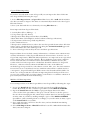
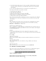
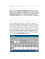
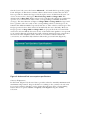
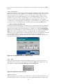
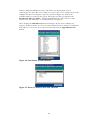
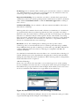
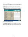
Technical report No 50
COPERT III
Computer programme to calculate
emissions from road transport
User manual (Version 2.1)
Chariton Kouridis, Leonidas Ntziachristos
and Zissis Samaras
ETC/AEM
November 2000
European Environment Agency
Cover design: Rolf Kuchling, EEA
Legal notice
The contents of this report do not necessarily reflect the official opinion of the European
Commission or other European Communities institutions. Neither the European Environment
Agency nor any person or company acting on behalf of the Agency is responsible for the use that may
be made of the information contained in this report.
A great deal of additional information on the European Union is available on the Internet.
It can be accessed through the Europa server (http://europa.eu.int)
©EEA, Copenhagen, 2000
Reproduction is authorised provided the source is acknowledged
Printed in Denmark
Printed on recycled and chlorine-free bleached paper
European Environment Agency
Kongens Nytorv 6
DK-1050 Copenhagen K
Denmark
Tel: +45 33 36 71 00
Fax: +45 33 36 71 99
E-mail: [email protected]
http://www.eea.eu.int
2
Initialisation
To initiate the software, use the following Logon data:
Name: copuser
Password: (blank)
i.e. no password required
Important information
The Recalculate All… button which is located on the right bottom corner of the
TOTAL results form and on the Fuel Balance form performs all necessary
calculations to produce the final emission results. Application of this button
introduces the effect of all changes to the activity data, emission factors and
advanced features to the final result. Also, in case the run has been compiled be
importing data from previous Copert versions, application of this button makes
sure that although activity data from the imported run will be preserved, all
emission factors and results will correspond to the new methodology. All other
Recalculate… buttons encountered in different forms should only be applied to
recalculate results only of the specific form.
3
Table of contents
Initialisation .................................................................................................... 3
Important information.................................................................................... 3
1.
Introduction........................................................................................... 5
2.
Requirements ........................................................................................ 5
2.1.
Software installed............................................................................................ 6
2.2.
Minimum hardware requirements .................................................................... 6
3.
Installing Copert III ................................................................................ 7
3.1.
Installation procedure...................................................................................... 7
3.2.
De-installation procedure ................................................................................ 8
4.
Structure of the program ...................................................................... 9
5.
Starting Copert III – Snap07 .................................................................. 9
5.1.
Menubar 1: Base menubar............................................................................. 10
5.2.
Menubar 2: Inventory menubar ..................................................................... 14
6.
A typical CORINAIR run....................................................................... 37
7.
Snap 08 – Off road machinery ............................................................. 38
7.1.
Menubars ...................................................................................................... 38
8.
Compact databases ............................................................................. 45
9.
Hot line................................................................................................ 46
4
1. Introduction
Copert III is an MS Windows* software program which is developed as a European
tool for the calculation of emissions from the road transport sector. An additional
module covers emissions from various off-road internal combustion engines. The
emissions calculated include regulated (CO, NOx, VOC, PM) and unregulated
pollutants (N2O, NH3, SO2, NMVOC speciation, …) and fuel consumption is also
computed. A detailed methodology supports the software application. For more
information regarding the methodology, the user should consult the Methodology
report. Copert III is an updated version of Copert II including both revised
methodological elements and a reworked user interface aiming at a faster
compilation of annual national inventories.
The new features of Copert III include an extended list of pollutants, the effect of
vehicle age (mileage) on emissions, an option to enable or disable the unleaded
gasoline allocation to pre-catalyst vehicles and others. Not all of those elements
are necessary for the compilation of annual national inventories. However, they
are of significant value when different scenarios need to be run for case studies.
This manual discusses all advanced features.
This report is designed in order to help Copert III users to produce in a short
time a complete annual national emission data set from road transport (and off
road machinery). Hence, the manual is divided in several chapters. The different
chapters include all information needed to build a complete data set, assuming
that the user has no former experience in using Copert III but he is quite familiar
with the methodology and the terminology used. A background knowledge in
using MS Windows is also expected, although no special skills are required.
Major attention has been given to ensure that no erroneous data are inserted. This
can certify reasonable results. It cannot guarantee their accuracy though, if input
data do not correspond to reality. This is a user responsibility.
In order to be compatible with the application, this manual is designed in the
same way that the software is developed. The contents in the manual are
structured in the same order as the respective forms appear when preparing the
inventory. Hence, it would be efficient to work with the program in parallel, as you
read the manual. This is a rather tutorial use of this book. In any case, you can
always refer to it for specific problems when you are quite acquainted with its use.
The following coding is used throughout the manual:
• Bold characters refer to a button, which you can click.
• Bold Inclined characters are used for fields in which you can click, enter, read
or select values. Alternatively they can symbolise a file.
• Inclined characters are used for text you have to type or they refer to chapter
names
• Underlined characters are used only to emphasise the context
*Microsoft, MS and Microsoft Access are registered trademarks and Windows and
Windows NT are trademarks of Microsoft Corporation
5
2. Requirements
2.1. Software installed
Copert III is a 32-bit application and 32-bit MS Windows platform (i.e. 95, 98, NT)
is required. Therefore, the software is not designed for operation in Windows 3.x
environment.
2.2. Minimum hardware requirements
1. IBM* – compatible computer Pentium100
2. 16Mb on board memory
3. Colour monitor 15’
4. Graphic card supporting 800 x 640 pixels screen resolution
5. Hard disk or network file server with 15 Mb free space
6. CD-Rom 4x or higher
7. Microsoft mouse or other compatible pointing device
It has to be noted that a faster processor based computer and/or more on board
memory are recommended if frequent use of the program is to be expected.
* IBM is a registered trademark of International Business Machines Corporation
6
3. Installing Copert III
3.1. Installation procedure
3.1.1. By Internet download
You can download the twelve (12) setup disks of Copert III from this web site:
http://vergina.eng.auth.gr/mech/lat/copert/copert.htm. All of the files are
compressed in a zip format and you have to decompress them by using Winzip or
Pkunzip.
The download and setup instructions follow:
1. Click on the links and download the three .zip files: disk1_4.zip, disk5_8.zip,
disk9_12.zip. They contain all 12 setup disks. Alternatively you may click the
CopertIII.zip which contains all necessary files in one zipped file (recommended
for fast Internet connections).
2. Extract the contents of the compressed .zip files in the same directory. A
temporary directory is recommended.
3. Delete the .zip files.
The downloading procedure has been finished. After steps 1-3, you must have 12
directories named disk# (where # from 1 to 12), each including several files that
have been extracted from the .zip files if you have downloaded the three
diskx_x.zip files or a single directory containing all the compressed files in case
you have downloaded CopertIII.zip.
4. In order to install the application, a typical Microsoft application setup
procedure has to be followed. Just double click file setup.exe (found in the disk1
directory) and follow the instructions given on-screen.
5. After the installation is complete, you may delete the 12 disk# folders, or store
their contents into disks (1.44 MB – 3½’), in order for the installation disks of
Copert III to be available for future use.
3.1.2. By set-up floppy disks
Copert III can be provided in 12 Windows set up disk files. Those set up disks will
install the application in your computer. The installation procedure is described
through the following steps:
1. Enter MS Windows. If you are already using Windows please make sure that all
of your MS Office applications have been terminated.
2. Insert in the 3½’ floppy disk drive the diskette labelled Disk 1.
3. Click the Start button and select Run…
4. In the field that pops up type x:\setup.exe, where x is the letter of the Floppy
Disk Drive.
5. Click the OK button
By doing so, you have entered a typical Windows application set up environment.
You can proceed with the installation as usually.
7
3.1.3. By set-up compact disk
Copert III can be also provided in Windows set up disk files stored in a CD-ROM.
Those set up disks will install the application in your computer. The installation
procedure is described through the following steps:
1. Enter MS Windows. If you are already using Windows please make sure that all
of your MS Office applications have been terminated.
2. Insert the CD into the CD-ROM drive.
3. Click the Start button and select Run…
4. In the field that pops up type x:\setup.exe, where x is the letter of the CD-ROM
Drive.
5. Click the OK button
By doing so, you have entered a typical Windows application set up environment.
You can proceed with the installation as usually.
After the installation procedure has been completed you are ready to start the
application.
Three new icons will have been added in the Start up menu. Click Snap07 or
Snap08 for compiling an inventory for Road Transport or Off Road Machinery
respectively. Refer to chapter 8 on how to use the Compact Databases icon.
3.2. De-installation procedure
To completely de-install the program from your computer:
On your Windows Task Bar select Start > Settings > Control Panel and double
click the Add/Remove Programs icon. From the list select Copert III. A typical
Windows De-installation procedure will follow. Select the Remove All option.
After doing so, Copert III will have been completely removed from your
computer.
8
4. Structure of the program
To have a better understanding of the program use it would be helpful to
familiarise yourself also with its structure. This chapter helps you use the software
more efficiently and take advantage of its special features.
The core of Copert III consists of two files named Snap07.mdb and Snap08.mdb
and correspond to Road Transport and Off Road Machinery respectively. The files
provide the user interface and include all the necessary modules to calculate
emission factors and emission results for Road Transport and Off Road Machinery
respectively. Importing from older Copert versions and exporting to ImportER are
also possible through those files. Finally they retrieve and save the data.
Snap0x.mdb are secured files. That means that the whole or parts of them cannot
be modified by third parties. The user has no access on the modules or the
routines of the program. For any problems you may encounter with the use and
attributes of those files you should better contact the developers.
In order to secure the program a special file – named copert.mda – has been
introduced from the older Copert II software. In this file all the necessary
information is included in a coded form. If you accidentally delete it then there is
no way you can use Copert III and you will have to re-install the application. You
can also contact the developers for a copy of copert.mda. Introducing the same
security information between Copert II and Copert III allows the trouble free
exchange of data between the two applications.
A list of the files that can be found in your Copert III directory follows:
File
Snap07.mdb
Snap08.mdb
Dobris.ico
Copexp.wk1
Compact.mdb
Description
Main database file for Road Transport
Main database file for Off Road Machinery
Icon
Lotus macro to export data from Copert90 runs
Compact Database file
Data97.xls
Copert.mda
Microsoft Excel file for importing Data in Excel format
File containing security information
After frequently using Copert III, you’ll notice that the main files size increases
and that calculations slow down. Those side effects occur because the structure of
the database is modified after multiple uses. To restore the original size and
performance of the database it is a good habit to often use the Compact Databases
application. This application is presented as an icon after you have installed the
application. More information can be found in chapter 8.
When you initially start any of the Snap07.mdb or Snap08.mdb files, they contain
no data. The data should be transferred into the system either by hand or by
importing from older Copert versions or importing from MS Excel. In any case,
the group of activity data, emission factors and results are termed as a run. Only
one run may be active each time – the current run. The current run can be edited
and updated and can be saved at any instance. No runs are kept in the SnapX.mdb
files but in separate databases, named by the user. Therefore, you may modify the
data directly in their respective store files. However, this is a delicate procedure
since any abnormal modification may harm the run and make it unreadable by the
core system files. Therefore, one should be very careful in changing only the
content and not the structure of the store files. For more information on the
structure of such files contact the software developers.
9
5. Starting Copert III – Snap07
You can start using the software by clicking on Snap07 from the task bar (Win9x,
NT 4.0). After doing so you will be encountered with a Logon dialogue box, which
is used for security reasons (Figure 1).
Figure 1: Logon box appeared when staring the application
In the Logon dialogue box enter copuser in the Name: field and leave the
Password: field blank. Click OK to proceed or Cancel to abort. The name used is
common for all Copert III users and has been transferred from Copert II.
An introductory form is presented after the OK button has been clicked, in which
all countries taking part in the CORINAIR inventory are present (Figure 2).
By clicking the About… button found on the bottom of the form you can obtain
information on how to receive solutions to any of the problems that might arise
while using the application. By clicking the OK button you are actually starting the
application.
Figure 2: Countries participating in the CORINAIR activities
5.1. Menubar 1: Base menubar
You are now introduced with a new feature of Copert III: the menubars. As soon
as you start the application a menubar appears (Figure 3) with two drop down
menus: File and Help.
10
Figure 3: Menubar 1 items
5.1.1. File
This item provides all tools to manipulate your inventory files. Under the File
menu item you can find the commands New, Open, Save, Save as…, Export to…,
Import from…, Close, Print…, Page Setup…, Print preview and Exit.
File>New
In order to create a new run, a standard Windows popup form will appear (Figure
4). You can then specify a name for the run and a folder to save it in. The program
will then start creating the necessary tables for storing the data of the new
inventory and a message appears on the screen as long as this process is active.
This may take a few seconds depending on your computer’s performance.
Figure 4: Open file dialog box
File>Open
If you have previously created a run in Copert III you can always view or edit the
data by selecting the Open menu item. A standard Windows popup form will
appear (Figure 4). Simply select the desired file or browse through the folders to
locate it. By clicking the Open button all saved data will be transferred into the
Copert III database and the selected run will become the current run.
File>Save
This command allows the user to save the current instance of the run anytime
during the inventory preparation. All updates brought into the inventory up to
this time will be saved and there is no way to retrieve data saved previously. This is
a major update compared to Copert II where the data could only be saved once
11
after the run had been completed. Additionally, if one wishes to preserve an older
version of the inventory, then the Save as… option (see below) needs to be used.
File>Save as…
If the user wishes to rename the inventory he is working on, or save it in a
different folder, this option prompts the user to do so via a standard Windows
popup form. By using this option you may create two versions of the same run and
preserve data you saved with the last File>Save command.
File>Export to…
This command exports the current inventory into two files cop_act.dbf and
cop_ef.dbf which include the activity data and the emission factors respectively.
Those files can then be introduced in CollectER via ImportER to link results
calculated with Copert III with the complete national inventory.
File>Import from…
You can import data introduced in inventories compiled with the older software
versions (Copert 90 and Copert II) by selecting this command. Also, when
inventory data are stored in Excel files you may also transfer them into the Copert
system. Below you may find information on how to import data in each of those
cases.
Copert 90 data importing
If you have already made a run of Copert 90 you can import the data of this run
into Copert III by following the steps:
1. Copy the copexp.wk1 file which is located on your Copert III installation
folder in the directory of the existing Copert 90 run.
2. Load Lotus
3. Retrieve the copexp.wk1 file and the program automatically creates the
copimp1.wk1 and copimp2.wk1 files.
4. In Copert III select File>Import from…>Copert 90 and first locate file
copimp1.wk1 and then file copimp2.wk1 by using twice the form of Figure 4.
The data are automatically transferred to the Copert III environment.
5. Save your data with the new format by selecting File>Save as….
Data imported from Copert 90 include:
1. Activity Data (Fleet, Mileage, …)
2. Usage Data (Speeds, Shares)
3. Evaporation Data (Evaporation Share, Fuel RVP)
4. Base Fuel Data (Consumption and not-advanced fuel specifications)
5. Temperatures and average daily trip distance
Imported data include do not include country name, emission factors (hot or
evaporative), cold start extra emission ratio or any data related to the advanced
Copert III characteristics. Temperature, RVP and daily trip distance are imported
as user specified values and become active in the software. The rationale of
importing data from Copert 90 is to estimate emissions according to the same
activity data used in the previous run but with the new Copert III methodology.
Therefore, one should not expect identical results between the Copert 90
inventory and the equivalent run in Copert III.
12
Copert II data importing
If you have already made a run of Copert II you can import the data of this run
into Copert III by following the steps:
1. Select File>Import from…>Copert II and first locate file *.mdb which includes
the data you want to import. The data are automatically transferred to the Copert
III environment.
2. Save your data with the new format by selecting File>Save as….
Data imported from Copert II include:
1. Activity Data (Fleet, Mileage, …)
2. Usage Data (Speeds, Shares)
3. Evaporation Data (Evaporation Share, Fuel RVP)
4. Base Fuel Data (Consumption and not-advanced fuel specifications)
5. Temperatures and average daily trip distance
6. Hot emission factors
7. Evaporation emission factors, where the user has provided own values. All other
values can be calculated in the software by using the Corinair Standard approach
and results will be the same with Copert II.
8. New technologies inserted by the user and their specifications
Imported data do not include country information, cold start extra emission ratio
and any information of the Copert III advanced characteristics. As in the case of
Copert 90, temperature, RVP and daily trip distance are imported as user specified
values and become active in the software. By recalculating evaporation emission
factors and cold start overemission ratios (but NOT hot emission factors) the
results of the hot and evaporation calculations should be identical to Copert II.
However, cold start related emissions will differ because of the different
methodology incorporated in each software version. Also, once hot start emission
factors have been recalculated, new hot emission values will be resulted and as a
consequence, Copert II and Copert III hot start related results will also differ. As
in the case of Copert 90, the rationale in importing data from Copert II is not to
preserve the results of the previous software version but to re-estimate emission of
past activity data with the new methodology.
MS Excel 97 data importing
You can import data of an Excel spreadsheet into Copert III by following the steps:
1. Locate the Data97.xls file which is located on your Copert III installation
folder. By default, the file contains a spreadsheet named DATAtoCOPERT.
2. Open the Data97.xls with the MsExcel program. Input data in the white
colored cells of the spreadsheet. The gray colored cells are locked to protect
the user from changing the file, which may result in data loss. You may produce
as many runs as you like by making multiple copies of the DATAtoCOPERT
spreadsheet (and renaming them accordingly) or you also make as many copies
of the Data97.xls file as you like.
3. Save (with any name) and close the file after you have finished introducing
data in Excel format.
4. Select File>Import from…>Excel97 and first locate file *.xls which includes the
data you want to import.
13
5. In the filed which will pop-up, select the spreadsheet which includes the data
you want to import. The data are automatically transferred to the Copert III
environment.
6. Save your Copert III run with the new format by selecting File>Save as….
Data imported from Excel spreadsheets include:
1. Activity Data (Fleet, Mileage, …)
2. Usage Data (Speeds, Shares)
3. Evaporation Data (Evaporation Share, Fuel RVP)
4. Base Fuel Data (Consumption and fuel specifications)
5. Temperatures and average daily trip distance
Imported data include neither emission factors (hot or evaporative) nor cold start
extra emission ratio. All relevant calculations need to be made in the Copert III
environment.
File>Close
This command erases all data of the current inventory and initialises the sofware
to start a new run. All data not previously saved in an external file (by using
File>Save as or File>Save as… will be lost!
File>Print, Page setup, Print preview
These commands are standard Windows commands and can be used the same way
as in all Windows programs to print different views of your results, set the margins
for the printed pages, etc.
File>Exit
To close Copert III simply click on this command. It is important to use this
command at the end of a session to erase all temporary objects from the Copert III
application file.
5.1.2. Help
Help>Contents and Index
This is a typical Windows Help environment, which includes the text of the User’s
Manual.
Help>Copert III on the Web
This command links you to the official site of Copert III via active Internet
connection.
Help>About Copert III
This command opens a form with information about COPERT III.
5.2. Menubar 2: Inventory menubar
Once the user has created, imported or opened a run a second menubar appears
(Figure 5) to help him add or edit the data of the current inventory.
Figure 5: Menubar 2 contents
This menubar has the following dropdown menus: Country, Activity Data,
Emission Factors, Results, Advanced, Add.
14
5.2.1. Country
Under the Country menu (Figure 6) you can find the commands Select…, Fuel,
Temperatures, Reid Vapour Pressure, Cold Start Parameters, Canister Efficiency.
Figure 6: Country menu item contents
Country>Select…
By selecting a country from the list on the Select Country form (Figure 7) you will
be proposed with available data for the country selected in the subsequent sessions
of the software, such as monthly temperatures, fuel vapour pressure, mean trip
distance, etc. When you need to add a country not included in the list then select
User and provide the name of the country in the subsequent pop-up form. Not all
of the countries have submitted official data in the previous Copert exercises,
therefore country-specific data are not available for each country in the list.
National experts are advised to contact the software developers when such data
become available (or need to be updated) to take it into account in future
versions of the software.
Figure 7: List of countries included in Copert III
Country>Fuel
By selecting Fuel under the Country menu, a Form appears (Figure 8) where the
user has to provide Data for the Fuel consumption and specifications to be used in
the calculations.
Four fuel types are included, specifically leaded and unleaded gasoline, diesel and
light petroleum gas (LPG). The fuel consumption provided by statistical
authorities has to be provided in the relevant fields on the top left corner of the
form while the content of fuel in different species and the hydrogen to carbon
atom ratio (H:C ratio) is provided on the bottom of the screen. Several values for
15
heavy metal content and H:C ratio are proposed. However, those values can be
changed if more accurate figures are available.
Two options are presented on the top right corner of the form, which can be used
to correct the results:
The first option (Is all gasoline consumed unleaded?) is relevant to inventories
performed for year 2000 and later in most EU member states, where according to
Directive 98/70/EC all gasoline consumed in the transport sector should be of the
unleaded type, which means that no Leaded fuel will be consumed by the vehicles.
When Yes is the answer to the question, then the statistical value for leaded
consumption will automatically be set to 0 and the default value for the unleaded
allocation calculations will be set to No.
The second option (Should unleaded gasoline be allocated to pre-catalyst
vehicles?) enables the user to decide whether the calculation should take on
board the unleaded fuel allocation to pre-catalyst passenger cars and is relevant to
pre-2000 corresponding inventories. The default value is Yes which means that
unleaded fuel allocation will take place. The unleaded allocation function
compares the unleaded fuel consumption calculated by Copert III on the basis of
relevant consumption factors (see § 5.2.3) with the statistical consumption
provided by the user. If the statistical value of unleaded fuel is larger than the one
calculated the reasonable assumption is made that some owners of pre-catalyst
vehicles operate their vehicles on unleaded fuel to benefit from the lower price. In
this case, a loop is performed where the gasoline type attributed to pre-catalyst
vehicles (which, by default, is considered as leaded) will change to unleaded until
the calculated consumption becomes equal or just larger than the statistical one.
The loop is performed with the order given in Table 4.5 of the Methodology
report. On the other hand, if the statistical unleaded consumption is less than the
calculated one, no changes take effect. The user can see which categories have
changed from leaded to unleaded AFTER the calculations have finished, under
the drop down menu Advanced>Unleaded Allocation.
Figure 8: Baseline fuel consumption specifications
16
On the lower left corner the button Advanced… is found which opens the popup
form of Figure 9. This form contains advanced fuel characteristics that the user
has to provide for future fuel types. On the right corner of this form the user can
choose between three fuel types: Base Fuel, Stage 2000 and Stage 2005. The
default value is Base Fuel. If this option is selected then all vehicles are assumed to
operate on a conventional – Base – fuel (corresponding to 1996 EU15 market
average). The introduction of improved Stage 2000 and Stage 2005 fuel types will
have a positive effect not only on the corresponding vehicle technologies to be
launched in 2000 and 2005 respectively but also to older vehicle technologies. The
fuel properties for base fuel cannot be modified by the user (default). However
fuel properties of Stage 2000 and Stage 2005 are proposed in the relevant fields
and can be also modified. Selection of any of the future fuel qualities corresponds
to an equal reduction of both the hot and cold start emission factors compared to
the base-case fuel. Sulphur values, which are relevant for advanced fuel use
corrections, are automatically transferred from the previous form (Figure 8).
Figure 9: Advanced fuel consumption specifications
Country>Temperatures
In this form (Figure 10) the user has to provide values for monthly minimum and
maximum temperatures. Proposed values according to the country selected exist
for several countries, but they can be changed by the user. The corresponding
button has to be pressed (User or Copert), with Copert being the default
selection.
17
Figure 10: Monthly minimum and maximum temperatures for cold start
calculations
Country>Reid Vapour Pressure
In this form (Figure 11) the user provides monthly values for the fuel Reid Vapour
Pressure in [kPa]. Again, here, values are proposed by Copert but the user can use
his own values by inputting them under the User Values column and pressing the
User Button on the bottom of the form.
Figure 11: Fuel reid vapour pressure used for evaporation calculations
Country>Cold Start Parameters
The ltrip value (mean daily trip distance) is introduced in this form (Figure 12) to
be used for the calculation of the Beta value. ltrip value corresponds to the mean
distance covered in trips started with an engine of ambient temperature (cold
start) and Beta is the fraction of the monthly mileage driven before the engine
and any exhaust components have reached their nominal operation temperature.
The estimated Beta value is calculated according to the equation given in the
methodology. In any case, the user may provide own values and use them by
clicking the User button on the bottom of the screen. Otherwise, the Copert
calculated values will be used.
18
In Copert III two different methodologies have been included for calculating
evaporation emission factors and, subsequently, evaporation emissions: the
Standard Corinair approach and the Alternative Approach. The Standard Corinair
is a transfer of the methodology exactly as applied in Copert II. The Alternative
Approach introduces a new methodology. More on the details of the two
approaches can be found in the methodology report, in sections 4.7.4 and 4.7.5.
The evaporation emissions in the Alternative Approach are calculated by applying
a canister efficiency on the evaporation emissions of uncontrolled vehicles. Two
efficiencies are assumed, one corresponding to pre-Euro II controlled vehicles
(Euro I and Euro II) and one corresponding to post-2000 controlled vehicle
technologies (Euro III and Euro IV). The canister efficiencies have been
calculated for each country of the EU 15 and for each month (Figure 13). The
user can provide his own values to be used by the program under the relevant
fields.
Figure 12: Cold start parameters
Note: Statistics collected in the framework of several projects (see Methodology Report) have shown that the
average ltrip distance at a European level is 12,4 km. Unless exact data are available, it is proposed to use
this value and not modify it in order to modify the results (i.e. to achieve a better fuel balance). The ltrip
value has a strong influence on the cold start emission estimates.
19
Figure 13: Canister efficiency for alternative evaporation calculations
Note: For those counties where no canister efficiencies are available, it is suggested that values
corresponding to a country of similar climate conditions may be used with good confidence.
5.2.2. Activity data
Under the Activity Data menu (Figure 14) you may find the options Fleet Info,
Circulation Info, Evaporation Share, Check>Driving Mode Share,
Check>Evaporation Share, Reports>(Fleet Data, Mileage Distribution, Vehicle
Speed, Evaporation Distribution, Slope Factor, Load Factor).
Figure 14: Activity data menu item content
Activity Data>Fleet Info
In this form (Figure 15) the user can input data for Population, Annual Mileage
(km/year) percentage of vehicles equipped with Fuel Injection and percentage of
vehicles equipped with Evaporation Control. To move between vehicle categories
two buttons on top of the form are placed. The Surrogate Population
Modification button gives the user the option to input the same number for
population for the current Vehicle Category. A similar button, for the mileage this
time, is the Surrogate Mileage Modification. The Multiply Mileage button
multiplies the Mileage by a constant value provided by the user. This option may
be of particular use when trying to obtain a better fuel balance. The Export to
Excel 97 button exports the current data to an Excel spreadsheet for further
processing or review.
20
Figure 15: Activity data collection form
Activity Data>Circulation Info
Figure 16 shows the input form aiming at collecting the average speed and the
mileage percentage driven by each vehicle technology per driving mode. Several
buttons on the bottom of the screen allow surrogate modifications of the speeds
and shares per driving mode for each vehicle category. Provide the value to be
introduced in all technologies of the current vehicle category in the pop-up form
after clicking each button. Also you may export all results in an Excel 97
spreadsheet by clicking the Export to Excel 97 button.
Figure 16: Circulation data collection form
21
Figure 17: Share of evaporation emissions to different driving modes
Activity Data>Evaporation Share
In this form (Figure 17) the user inputs the distribution of evaporative emissions
to different driving modes. Similar to the previous forms, Surrogate Modifications
and Export to Excel 97 options are activated with use of the respective buttons on
the bottom of the screen.
Activity Data>Check…
After you have entered the mileage and evaporation share to the different driving
modes it is obvious that they should sum up to 100%. All non-zero records not
summing up to 100% can be identified by use of the form given in Figure 18
which is presented when the Check… option is selected. You may correct any of
the Urban, Rural and Highway value in order to bring the Total to the range of
100% (maximum deviation 0,5% allowed).
Figure 18: Driving mode share checking form
Activity Data>Reports
You may print summary reports on the Fleet Data, Mileage Distribution, Vehicle
Speed, Evaporation Distribution, Slope Factor, Load Factor data by selecting this
option. You may first have a preview of the reports under this drop down menu
and then you can print the selected ones by following a standard printing
procedure.
22
5.2.3. Emission and consumption factors
Under the Emission Factors menu (Figure 19) you may find the commands Hot
Stabilised, Excess Cold Emission and Evaporative.
Figure 19: Emission factors menu item contents
Emission Factors>Hot Stabilised
The spreadsheet-like form (Figure 20) provides a general view of the Hot
Stabilised Emission Factors under three different columns (Urban, Rural,
Highway). Those emission factors correspond to vehicle emissions when the
engine and exhaust components have reached their nominal operation
temperature. Only emission factors corresponding to non-zero-population of
vehicle categories and vehicle technologies will be shown. The list of pollutants on
top of the form is used to select emission factors for the different pollutants.
Included in the list is also the fuel consumption for stabilised engine temperature
(FC). Emission factors can be exported to Excel 97 by clicking the Export to Excel
97 button. The Recalculate… button on the right bottom corner of the form
executes the modules to calculate the hot emission factors in case the user has
made changes during the session.
When one wishes to introduce own emission factors and not use the values
proposed by the software, the Keep check box needs to be selected next to the
emission factor value introduced for any vehicle technology. In the subsequent
calculations the original value given by the user will be used by the program, with
no additional corrections (for mileage degradation, load and slope effect and so
on). This value will not be changed when recalculating results. In order to restore
this emission factor to the Copert III calculated value you need to deselect the
Keep option and recalculate the emission factors.
Figure 20: Hot emission factors results form
23
Emission Factors>Excess Cold Emissions
This spreadsheet-like form (Figure 21) is of the same principals as the hot
emission factors form. However, cold excess emission factors are temperature
dependant and therefore an additional list of months (January to December) is
given on the top of the form except of the list of pollutants and fuel consumption
given below. The Keep… function is similar to that described in the previous
paragraph.
Since Excess cold emissions are initially attributed to urban driving only, assuming
that the majority of vehicle start their trips from urban areas, only urban emission
factors are proposed for cold start.
Emission Factors>Evaporation>Standard Corinair
In this spreadsheet-like form (Figure 22) the user can edit the emission factors for
fuel evaporation being calculated with the standard Corinair methodology
originating from different vehicle sources and covered by the six buttons on the
top of the form. Those emission factors are only relevant for gasoline powered
vehicles. Two columns are provided, proposing emission factors for vehicles
equipped with evaporation control systems (Controlled) or without any control
devices (Uncontrolled). Again, own emission factors may be preserved by selecting
the Keep… check box for any vehicle technology and evaporation source. The
Standard Corinair approach results in overestimated Hot Soak losses for
uncontrolled vehicles, compared to new experimental data. However, in order to
preserve consistency with older Copert versions, this original approach has been
transferred to the new software version.
Figure 21: Cold start excess emission factors results form
Emission Factors>Evaporation>Alternative Approach
A similar form to Figure 22 is proposed for evaporation emission factors in the
case of the Alternative Approach. Details on this approach can be found in the
methodology report. In this apporach, since no distinction is made to warm and
hot soak losses and to losses from carburettor or fuel injection equipped vehicles,
only three buttons are present on the top of the form (Diurnal, Hot Soak,
Running Losses). Evaporation emission factors calculated with this option are
24
again only relevant to gasoline powered vehicles. It is assumed that all vehicles up
to the Open Loop technology are uncontrolled and all three-way catalyst
equipped vehicles are controlled ones.
Furthermore, a distinction is made to controlled vehicle technologies with regard
to their canister efficiency. In those cases where the Base Fuel has been selected
(Figure 9) two different canister efficiencies are assumed for pre-2000 and post2000 controlled vehicle technologies because of the different evaporation control
legislation valid for the different technologies. In the cases where either Stage
2000 or Stage 2005 fuel grades have been selected, the canister efficiency is the
same for all controlled vehicle technologies (corresponding to post-2000 values)
because of the maximum summer RVP value (60 kPa) introduced with Directive
98/70/EC. With regard to the interface details of the form, two columns are
provided, proposing emission factors for vehicles equipped with evaporation
control systems (Controlled) or without any control devices (Uncontrolled).
Values introduced in the Controlled case for pre-Euro I vehicles and in the
Uncontrolled case for post-Euro I technologies are neglected. Again, own
emission factors may be preserved by selecting the Keep… check box for any
vehicle technology and evaporation source.
Figure 22: Evaporation factors results form
5.2.4. Results
Under the Results menu (Figure 23) you may find the commands Hot Stabilised,
Cold Excess, Evaporation, TOTAL, Fuel Balance, NMVOC Speciation and Run
Details.
25
Figure 23: Results menu item contents
Results>Hot stabilised
Figure 24 presents the form of the hot emission results according to pollutant,
driving mode and vehicle technology. Results are presented in tonnes for all
major gaseous pollutants and in kg for heavy metals. The user can move between
different pollutants by selecting them in the list located on top of the form. The
Recalculate… button introduces to the results any changes brought to the Fleet
Info data or directly to the emission factors. No emission factors are recalculated
with this action and advanced Copert III characteristics modifications are
introduced in the software. The Export to Excel 97 button exports results to Excel
format.
Figure 24: Hot emissions results form
Results>Excess cold
Figure 25 presents the total excess emissions produced during the engine
operation under transient thermal conditions. Although only an urban emission
factor has been proposed for excess cold emissions, total emissions during
thermally transient engine operation can also be allocated to rural driving in
special circumstances. Those special cases are thoroughly discussed in the
methodology and the applied algorithm for the allocation of cold start excess
emissions in different driving modes is given on chapter 4.6 of the Methodology
report. Similarly to the previous case, the Recalculate… button needs to be clicked
to introduce any changes. Similar to the hot emission factor case, the
Recalculate… button does not recalculate the cold overemission values, in case
that any of the activity data have been changed. Results may also be exported to
Excel by clicking the respective button.
26
Figure 25: Cold start related results form
Results>Evaporation
This form (Figure 26) presents the emission results due to fuel evaporation in tons
according to driving mode and evaporation source. Fuel evaporation emissions
contribute to the total NMVOC vehicle emissions. The evaporation share
distribution specified in the activity data is used to allocated evaporation emissions
to different driving modes. Again, results are updated by clicking the
Recalculate… button and can be exported to Excel 97 by means of the respective
button.
Figure 26: Fuel evaporation results form
Evaporation results are calculated either with the Standard Corinair or with the
Alternative Approach. To choose between one of the two methods, you need to
27
calculate the respective emission factors as described previously. Results are
automatically calculated according to the selected method.
Results>TOTAL
This form (Figure 27) presents the TOTAL emission and fuel consumption results
(i.e. the sum of Hot stabilised, Excess Cold and Evaporation emissions) in tons for
gaseous pollutants, consumption and PM and in kg for heavy metals. The user can
move between different pollutants by selecting them in the list located on top of
the form. The two buttons located on the bottom of this form (Emission Source
Oriented, Driving Mode Oriented) are used to preview printable summary reports
on total emissions according to driving mode (urban, rural, highway) or emission
source (hot, cold, evaporation) respectively. Similar reports were also produced in
Copert II. Additionally, the Multiple Reports button allows the user to directly
print several reports by selecting the respective fields in a pop-up form. Also, all
results calculated can be exported to Excel by selecting the respective button.
Note: The Recalculate All… button located on the right bottom corner of the form performs all necessary
calculations to produce the emission results. Application of this button introduces the effect of all changes to
the activity data, emission factors and advanced features and one may be sure that the final values of the
calculations are provided when clicking this button. However, this action needs to be made again if further
changes to any of the activity data or emission factors have taken place. Also, in case the run has been
compiled be importing data from previous Copert versions, application of this button makes sure that
although activity data from the imported run will be preserved, all emission factors and results correspond to
the new methodology. This action may take several seconds depending on the computer used.
Figure 27: Totals (hot & cold start & evaporation) results form
Results>Fuel Balance
The fuel balance (Figure 28) provides a control point to compare the statistical
fuel consumption provided in the respective form (Figure 8) with the total fuel
consumption calculated by the software. The deviation between the two values
should not exceed a few percentage units for the input data to be considered
representative of their application. Therefore, this check can provide a verification
of the overall accuracy of the input data and that no severe inconsistencies have
been introduced into the calculations.
If a significant deviation exists between the two values then you should make sure
that the statistical fuel consumption has been introduced correctly and it
corresponds to the real amount of fuel consumed by vehicles operating in the area
selected for the inventory. If this figure is correct then some of the activity data
28
need modifications. To obtain a better match between the statistical and
calculated fuel consumption one may propose:
•
•
•
•
Modify the mileage fraction allocated to different driving modes (Figure 15).
Emission and consumption factors vary according to driving mode and
therefore wrong estimations of the distance travelled under different
conditions may provide an erroneous final result.
Modify the speeds attributed to different driving modes. Speeds introduced in
the relevant fields of Figure 16 correspond to the mean travelling speeds for
the fleet of vehicles and have a significant influence on the emission and
consumption factors.
Make sure that the vehicle fleet has been correctly distributed to different
vehicle technologies (Figure 15). Significant estimations may be necessary to
adapt different national classification (especially before Euro I vehicles) to the
vehicle technology classification of Copert III. Since different vehicle
technologies have both different emission and consumption factors, the
particular allocation of vehicles has an impact on the also final result.
Although the mileage driven per year has a linear effect on the total emissions,
this should be a relevantly evident figure which accepts minor modifications.
Moreover, values like monthly temperatures, RVP, etc. although have an effect
on total emissions should not be changed because they should be considered
much more reliable in comparison with those previously mentioned.
Figure 28: Fuel balance (statistical and calculated) results form
Additionally, it needs to be mentioned that emissions of fuel dependant pollutants
(CO2, SO2, Heavy Metals) are calculated on the basis of the statistical fuel
consumption. To do so, the total emissions, as calculated by Copert III with
application of the fuel consumption factors, are multiplied by the ratio
Statistical/Total Calculated fuel consumption for each fuel type. In order to apply
this correction, the statistical fuel consumption needs to be introduced. In case
the relevant figures miss, the user is prompted to provide them by the message
box of Figure 29. You should click Yes if you want to provide the statistical fuel
consumption for the specific fuel type or No to ignore the correction and
calculate results on the basis of the calculated fuel consumption only. Naturally, if
the No option is chosen, this would mean that no statistical consumption figures
exist for the specific fuel type, therefore the fuel balance is not valid.
Figure 29: Information message in case of zero statistical consumption
29
Results>NMVOC Speciation
This form given in Figure 30 provides the total NMVOC speciation in different
hydrocarbon species originating both from exhaust and evaporation emissions.
The upper part of the form presents the emissions of open chain and aromatic
hydrocarbons in [t] and the lower part the total emissions of PAHs and POPs
(including furans and dioxins) in [g]. Please note that the speciation does not
include 2-stroke engines and that, when summed up, the NMVOC species list gives
a lower value than total NMVOC emissions because some of NMVOC is
considered to be PAHs and POPs. The total calculated when summing up the
NMVOC list is equal to the fraction given in Table 5.36b of the Methodology
report.
Figure 30: NMVOC species list and corresponding contribution
Results>Run Details
The form of Figure 31 provides a summary of the current run and lists some of its
basic characteristics such as Name, Date, Country selected. It also shows which
parameters have received Copert or user values, what assumptions have been
made for the leaded/unleaded gasoline used and which corrections (e.g. Load,
Slope, IM effect) have been introduced in the calculations. It also shows on what
fuel specifications (1996 Market Average, Euro 2000 or Euro 2005) have been
based the calculations. For the advanced features, a detailed description is given in
the following sections.
30
Figure 31: Summary information of active run.
5.2.5. Advanced
Under the Advanced menu (Figure 32) one may find the following options:
Reduction Percentage, Mileage Degradation, Load Effect, Slope Effect, Unleaded
Allocation, Correction Coefficients>Load Correction, Correction
Coefficients>Slope Correction, Correction Coefficients>Mileage Degradation IM,
Correction Coefficients>Mileage Degradation No IM. These advanced features of
Copert are not necessary for the compilation of a standard national inventory.
They are used to refine the results and provide additional sensitivity parameters by
implementing a more detailed description of the activity characteristics such as the
load factor of the HDV or the road gradient etc. Also, default reduction
percentages for future vehicle technologies may be introduced by the user if
alternative estimations are made and the introduction of an improved Inspection
and Maintenance scheme may also be modelled.
Figure 32: Advanced menu item contents
Advanced>Reduction Percentage
The reduction percentages for hot emission factors of all post EURO I
technologies are driving mode and pollutant dependent. The reduction
percentages express the decrease of the hot emission level of recent and future
31
vehicle technologies over the EURO I emission level depending on the pollutant
considered. Although an inclusion of Euro V passenger cars has been
accommodated, no estimation for their emission level can be done and therefore
a default reduction of 100% has been introduced which should be changed by the
user when experimental data become available.
Advanced>Mileage Degradation
The form of Figure 33 is used to collect the mean cumulative fleet mileage in
kilometres for each vehicle technology. In other words, the mean distance
travelled by the fleet vehicles of the specific technology level since their
introduction in the market. This value is then used to provide an emission
degradation factor depending on vehicle age (or, total mileage driven). Relevant
degradation factors are only given for EURO I and later passenger cars and light
duty vehicles only and apply to hot emissions only. The user may select between
three options on the bottom of the screen:
No: No degradation factors are calculated and therefore no correction of the
baseline hot emission factors is introduced.
With NO IM effect: If this option is selected then the degradation factors are
calculated assuming that the applicable Inspection and Maintenance scheme is
similar to Directive 92/55/EEC.
With IM effect: In this case, degradation factors are calculated assuming that an
improved Inspection and Maintenance scheme is in place.
For more details about the IM effect you may refer to the methodology report.
Figure 33: Mean fleet mileage collection form
Advanced>Load Effect
The load percentage corrections are applicable to heavy duty vehicles only and
they depend on the vehicle gross weight class and driving mode. A default value of
50% is given and this corresponds to the baseline emission factors of Copert. In
order to apply a different load percentage you need to select the Yes option once
you have made your changes. To remove the effect of different load percentages
just select the No option. Needless to say that load percentages should range
between 0 and 100 denoting a totally empty or a fully laden vehicle respectively.
32
The load correction factors are automatically calculated when you press the OK
button.
Advanced>Slope Effect
In this form (Figure 34) the user provides the mean gradient class of the road for
different vehicle categories (HDV only) and different driving modes. Click on the
drop down menu of each vehicle category to select between 5 gradient classes
ranging between -6% (uphill driving) to +6% (downhill driving). The 0% slope
value means that no changes will be made to the baseline emission factors (even
road) even if the user has clicked the Yes button. The different road gradient
corrections are only applicable for a limiting – and reasonable – speed range. The
correction factors are automatically calculated when you press the OK button.
• Advanced>Unleaded Allocation
This form provides information on which vehicle categories the fuel type used has
been shifted from Leaded Gasoline to Unleaded Gasoline during the Unleaded
Allocation algorithm. The form provides two columns, one with the Default Fuel
Type which is assumed prior to unleaded allocation and one under the New Fuel
Type name which provides the fuel type considered after the unleaded fuel
allocation to pre-catalyst vehicle technologies. The changes are temporary and can
be cancelled if a different value is given for the statistical consumption of
unleaded fuel or in case that the unleaded allocation is cancelled by means of the
relevant field in Figure 8.
Figure 34: Introduction of mean slope of roads
5.2.6. Add
This menu item should be used when additional vehicle categories to the ones
offered by Copert need to be introduced. Under the Add menu (Figure 35) one
may find the commands New Technology and New Subsector.
Figure 35: Add menu tem contents
Add>New Subsector
This option may be used when a new subsector needs to be introduced under one
of the five main vehicle sectors (Passenger Cars, Light Duty Vehicles, Heavy Duty
33
Vehicles, Mopeds and Motorcycles). The subsector may include several
technologies. To introduce a new subsector you need to select a name in the form
of Figure 36 after selecting the respective option in Figure 35. A list of the
available subsector names is also given. The name you have provided in the
Provide new subsector name… field should NOT be the same with any of the
names in the list. Otherwise, a warning message will appear.
After clicking the Add Subsector button in Figure 36, the form of Figure 37
appears. In this form the user chooses under which Sector he wishes to classify the
new Subsector. Select the Sector from the list and click the Append Subsector…
button.
Figure 36: Introduction of new subsector
Figure 37: Sector on which to base new subsector
34
Figure 38: New technology name
In the next step you need to introduce a new technology to be appended in the
new subsector. This is made by means of the form in Figure 38. You need to
provide a name for the new technology in the field on the bottom of the form
which should not much any of the given names of the default technologies
included in the Copert III database structure and click the Add button. This has
been decided to avoid conflicts of the new with the existing technologies.
After appending the new Technology you need to provide several information
elements which will be used in the subsequent calculations. Those are collected by
means of the form given in Figure 39. The necessity of the several fields included
is described in the following.
Figure 39: New technology characteristics
Fuel Type: choose the Fuel Type used for this vehicle category. This is used to correctly allocate
the consumption of the specific technology.
35
Technology: choose whether this technology is conventional, catalyst or a 2-Stroke
one. This information is required to accurately allocate the emissions of the new
technology when exporting results to ImportER.
Evaporation Modelling: choose whether you wish to calculate fuel evaporation
emissions for this new technology. Evaporation emission factors will be calculated
either with the Standard Corinair or with the Alternative Approach according to
user’s choice.
Cold Start Modelling: choose whether cold start emission should be allocated to
this vehicle technology.
With regard to hot emission factors and cold start overemissions, no calculations
are performed for this new technology but the user has to provide own values.
This is because the actual vehicle technology for this new technology is not known,
therefore no estimation may be made a-priori. On the other hand, concerning
fuel evaporation, emissions due not depend on vehicle technology, other than the
distinction to controlled – uncontrolled case. Therefore, evaporation emission
factors are calculated for the new technology.
Fuel Tech: choose the enabling fuel technology for the specific vehicle
technology. Select conventional fuel (for a technology introduced up to 2000),
Stage 2000 fuel if the specific technology is of the same age with Euro III vehicles
or Stage 2005 fuel if the new vehicle technology is compatible with Euro IV
emission standards.
Use this fuel for unleaded allocation checkbox: once checked, this technology, if
leaded, will take part to the algorithm for changing the leaded to unleaded fuel
during the unleaded allocation calculations. This technology will be changed first,
if unleaded allocation is required.
Add>New Technology
In the case you only need to introduce a new technology in one of the existing
Sectors and Subsectors then use the second option of the form given in Figure 35.
You will then be proposed with the form of Figure 40 in which you need to select
the Sector and thereafter Subsector to append the new technology.
Figure 40: Alternative form when new technology is introduced
After clicking the OK button in Figure 40 you need to follow the same procedure
as previous through forms of Figure 38 and Figure 39.
36
6. A typical CORINAIR run
In order for Copert III to export results into the CollectER system via ImportER, it
produces two files (see §5.1.1). The minimum number of input data necessary for
the creation of a complete road transport inventory is met when providing correct
data for the following fields:
1.
2.
3.
4.
5.
6.
7.
Country>Fuel
Country>Monthly Temperatures
Country>Reid Vapor Pressure
Country>Cold Start Parameters
Activity Data>Fleet Info
Activity Data>Circulation Info
Activity Data>Evaporation Share
By default, the Corinair Standard approach is considered for evaporation emission
calculations. In case you need to introduce the Alternative Approach you also
need to check the Country>Canister Efficiency fields and calculate the new
emission factors by selecting Emission Factors>Evaporation>Alternative Approach.
The calculation of the results and the compilation of this “Typical CORINAIR
run” may be concluded by selecting the Calculate All… button found under the
Results>TOTAL or Results>Fuel Balance options. After following those steps,
results are ready to be exported in the CollectER format. Obviously, all other
Copert III features (such as advanced fuel characteristics, mileage degradation,
slope and load corrections) may be applied to refine calculations but are not
necessary to perform the typical run.
37
7. Snap 08 – Off road machinery
This chapter assumes that you are already familiar with the use of the software by
having compiled at least one Road Transport inventory. This means that you can
open and manipulate a run, add and edit data and produce results. This chapter
only demonstrates the necessary steps you have to take in order to include off road
machinery data and emissions in your run.
To enter the off road module you have to select Snap08.mdb from the Windows
Start menu.
7.1. Menubars
Two menu bars are available for using the Snap08 application. The Base menubar
provides similar but more simplified operations with the one presented in chapter
5.1 for Snap07 and it is not further discussed in the following. The Inventory
menubar is shown in Figure 41and will be thoroughly examined
Figure 41: SNAP 08 Menubar items
7.1.1. Fuel
Under the Fuel menu item you can find the command Fuel Specifications.
Fuel>Fuel Specifications
As in the case of Snap 07, the specifications of the fuels used are necessary to
compute the emissions produced by the fuel content in several elements. To do
so, click the menu item Fuel Specification. This reveals the form of Figure 42. No
statistical consumption has to be provided in this case because there is no fuel
balance in the case of Snap 08; only fuel content in Lead and Sulphur. The H:C
ratio of the fuel is also necessary for the calculation of CO2 emissions.
Figure 42: Fuel specifications collection form
Enter the necessary figures for the Diesel, Gasoline and LPG fuels and click OK to
exit.
7.1.2. Activity Data
Under the Activity Data menu item you can find the commands N, HRS, LF,
Power Distribution, Age Distribution, Diesel Type Mix.
38
Activity Data>N, HRS, LF
Selecting the menu item N, HRS, LF will lead you in the form shown in Figure 43.
The different fields are described next:
Vehicle population: Enter the number of vehicles (engines) of the specific
category
Annual Working Hours: Enter the working hours for each machinery type for the
time scale of application (e.g. annual working hours, seasonal working hours, etc.)
Load Factor (%): An estimation of the average work load factor of the vehicles
Figure 43: Activity data collection form
Activity Data>Power Distribution
Power Distribution (kW): Enter the percentage distribution of each machinery
type into several power output categories (Figure 44). The emissions of the
different machinery differs for different power classes. Notice that the program
will not let you provide a distribution that does not result in a sum of 100%.
39
Figure 44: Power distribution collection form
Activity Data>Age Distribution
Age Distribution: Provide the distribution of the vehicles into different age classes
(Figure 45). The application of special degradation factors will be possible if the
age of the vehicles is known. The sum of the age distribution figures should also
equal 100% in this case.
Figure 45: Age distribution collection form
Activity Data>Diesel Type Mix
Concerning diesel fuelled engines, the emissions vary according to the engine’s
combustion layout. This means for example that a turbocharged direct injection
engine probably has a different emission level than a natural aspirated
prechambered one. To compensate for those irregularities different emission
40
factors have to be applied. As a result, the number of diesel engines for each
layout has to be entered.
This is done with the help of the form in Figure 46. You have to enter the engine
percentage distribution at the different concepts in the fields provided for that
reason. Notice that the sum must be 100%. With the navigation buttons you can
go through all of the vehicles of the current collection equipped with diesel
engines. For each category, the diesel type distribution has to be entered for all
power classes. To select a power class for vehicles of a specific category use the
buttons at the right hand side of the form.
7.1.3. Emission Factors
Under the Emission Factors menu item you can find the commands Baseline,
Degradation, Evaporation, Weighting.
Emission Factors>Baseline
Engines of different power output produce different amount of pollutants for
each hour of use. This leads to the necessity of the introduction of different
emission factors for each pollutant, type of fuel and power class. Those emission
factors can be entered in the form presented after the menu item Emission
Factors>Baseline has been clicked (Figure 47).
Again, emission factors (g/kWh) are proposed for each fuel. You can change
those values if more updated data are available. You can select different fuels with
use of the navigation buttons at the top of the form.
Figure 46: Fractions of different diesel combustion systems
41
Figure 47: Baseline emission factors for different pollutants
Emission Factors>Degradation
The degradation factors can be found under the menu item Degradation. Those
degradation factors depend on the pollutant and the fuel used. They express the
expected degradation percentage of the engine per year (Figure 48).
Figure 48: Degradation factor to compensate for machinery age
Emission Factors>Evaporation
Vehicles equipped with gasoline engines contribute to the total emissions also due
to evaporation effects. You have to provide emission factors for evaporation from
gasoline engines. The form of Figure 49 is used for that reason. Provide the
emission factors at the respective field. For vehicles in the same subsector, select
between 2 stroke and 4 stroke engines by using the respective buttons G2S and
G4S at the top of the form.
42
Figure 49: Fuel evaporation factor for gasoline engines
Evaporation emission factors are proposed for both engine types. You can either
keep the values proposed or enter your own.
Emission Factors>Weighting
The emission factors already presented in the previous paragraphs are baseline
emission factors. This means that they are common figures for each pollutant, fuel
used and power class. In the case of diesel engines, as has already been
mentioned, a more detailed specification is necessary, according to the
combustion layout of the engine. Different type diesel engines present different
emission levels.
If the same emission factors have to be used for all diesel engines (baseline
emission factors), they have to be corrected with special correction or weighting
factors. Those special factors are function of the pollutant concerned and the
combustion layout applied. To view or change those emission factors, click the
Weighting menu item in order to show the form of Figure 50.
The titles in the first row are the initial letters of the concept applied. You can
move between the different stages of diesel emission legislation with use of the two
buttons placed at the form’s top. You can also change the values at will.
7.1.4. Results
Under the Results menu item you may find the command Off Road Results.
43
Figure 50: Weighting factors according to diesel combustion system to
correct baseline emission factors
Results>Off Road Results
The Off Road Results menu item will activate the procedure of calculating
emission results. The emission results are presented in the respective form. You
can select the pollutant of interest with the buttons at the top of the form. You can
recalculate the results by clicking on the Recalculate button.
On the bottom of the screen the Report button is available. By clicking on this
button the form (Figure 51) appears. On this form there are two button options:
Fuel Oriented: Preview a printable report including fuel aggregated results for the
current pollutant.
Sector Oriented: Preview a printable report with results summed up on the basis
of the different sectors entered.
You can move through the different pollutants by clicking on the drop down
menu next to the Pollutant label.
Figure 51: Form to select report to view
44
8. Compact databases
If you often use Copert III you may notice that the two main files Snap07.mdb and
Snap08.mdb considerably increase in size. To correct this you can run the
Compact Databases application found in the task bar under the Copert III folder
(Win9x, NT 4.0).
A standard Windows form will appear. (Figure 4). The user will then be asked to
locate the desired file, Snap07.mdb or Snap08.mdb, to compact. This application
restores the original size of these two files. Since a standard database repairing
procedure is also initiated when you use this application, also try the Compact
Databases option if you encounter any erroneous operation of the Snap07.mdb or
Snap08.mdb files. If the problem persist then you should contact the Copert HotLine.
9. Hot line
In case you need assistance with installing and running the application, contact:
Chariton Kouridis e-mail: [email protected], tel: +3031 996051
Leonidas Ntziachristos e-mail: [email protected], tel:+3031 996061
Zissis Samaras e-mail: [email protected], tel: +3031 996014
46