1
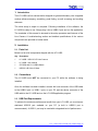
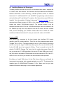
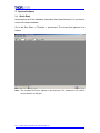
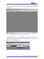
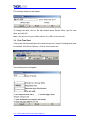
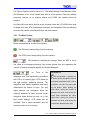
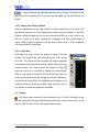
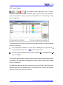
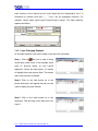
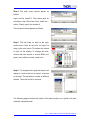
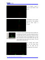
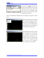
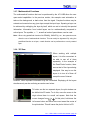
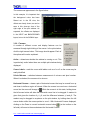
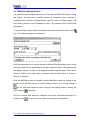
Operation Manual Thorlabs LC1 - USB USB 2.0 CCD Line Camera 2005 Version: Date: 2.0 28-Nov-05 Copyright© 2005, Thorlabs GmbH, Germany Contents Page 1. Introduction 10 2. Installation 10 2.1. Parts List 10 2.2. Connections 10 2.3. USB Port Requirements 10 2.4. Installing the Application Software 11 2.5. Installing Software for Developers 12 3. Spectra Software 13 3.1. Quick Start 13 3.2. First Time Start 15 3.2.1. The Main Toolbar 16 3.2.2. Getting Your First Line Scan 17 3.2.3. Scroll Bars 17 3.3. Layers 17 3.3.1. Layer Control 18 3.3.2. Layer Changing Example 19 3.3.3. Current Layer 22 3.3.4. Averaging & Smoothing 22 3.3.4.1. Averaging 22 3.3.4.2. Smoothing 22 3.3.5. Peak Finder 23 3.3.6. Gaussian Transform 23 3.3.6.1. Gaussian Plot 24 3.3.6.2. Gaussian Distribution of a Beam 24 3.3.7. Mathematical Functions 28 3.3.8. 3D View 28 3.3.9. Cursors 29 3.4. Storing and Retrieving Data 30 3.5. Multi-Save Storage Feature 31 3.6. Collecting Event Driven Data using Ext. Trigger Mode 32 4. Troubleshooting 32 4.1. In the Win2000 and XP Operating System 32 4.2. In the Win98 and ME Operating System 33 4.3. Run the LC1-USB Program 33 5. LC1-USB Specifications 36 5.1. Dimensions 37 6. Addresses 38 7. Warranty 39 7.1. WEEE 40 7.1.1. Waste treatment on your own responsibility 40 7.1.2. Ecological background 41 We aim to develop and produce the best solution for your application in the field of optical measurement technique. To help us to come up to your expectations and develop our products permanently we need your ideas and suggestions. Therefore, please let us know about possible criticism or ideas. We and our international partners are looking forward to hearing from you. Thorlabs GmbH This part of the instruction manual contains specific information on how to operate an LC1 – USB, USB 2.0 CCD Line Camera manually and by remote control. *Attention* This manual contains “WARNINGS” and “ATTENTION” label in this form, to indicate dangers for persons or possible damage of equipment. Please read these advises carefully! NOTE This manual also contains “NOTES” and “HINTS” written in this form. 1. Introduction The LC1-USB is a line camera that is designed for general laboratory use. Integrated routines allows averaging, smoothing, peak finding, as well as saving and recalling data sets. The initial setup is simple to complete. Following installation of the software, the LC1-USB is ready to use. Simply plug it into a USB 2.0 port and run the application. The remainder of this manual is devoted to the setup procedure and features of the Line Camera. A troubleshooting section and detailed specifications of the various components are provided to further assist. 2. Installation 2.1. Parts List Below is a list of all components shipped with the LC1-USB: Qty. Description 1 LC1-USB - USB 2.0 CCD Line Camera 1 LC1-USB - User Manual 1 CD-ROM with LC1-USB Software 1 USB 2.0 A-B Cable, 2 Meter 2.2. Connections The LC1-USB must NOT be connected to your PC while the software is being installed. Once the software has been installed, connect the host connector of the USB cable to the USB 2.0 port ( or USB 1.1 port ) on your PC and the device connector of the USB cable to the LC1-USB and run the LC1-USB application program. 2.3. USB Port Requirements To achieve the maximum performance benefit from your LC1-USB, you must have a dedicated USB 2.0 port available on your PC ( a built in USB 2.0 port is recommended ). A USB 1.1 port may be used with a degraded level of performance. LC1 – USB / USB 2.0 CCD Line Camera/ Page 10 2.4. Installing the Application Software Insert the CD-ROM. The Installation Menu program should launch automatically and show up with: If not, browse to the CDROM directory \Autorun and run the program Autorun.exe. Mouse click on the “Install Software” menu button to install the application program “Spectra”. To install the USB driver for the LC1-USB, make sure the LC1-USB is NOT plugged-in to a USB port then click on the “Install Jungo” menu button. For Windows 9X systems, the menu program cannot be used to install the driver. Instead, open a DOS window and CD to the CDROM directory \USB\Utilities and run the batch program man_install_9x.bat. LC1 – USB / USB 2.0 CCD Line Camera/ page 11 2.5. Installing Software for Developers Thorlabs provides instrument drivers (API) for developers who want to integrate the LC1-USB in their own software. The instrument drivers provided here are based on National Instruments™ VISA technology. Thorlabs provides a driver for National Instruments™ LabWindows/CVI™ and LabVIEW™ programming environments as well as for Microsoft™ and Borland™ compilers. All of these drivers need VISA to be installed. From the website of National Instruments™ (www.ni.com/visa) you can download two different versions of VISA (a fully featured version “NI-VISA” and a runtime only version “VISA-Runtime engine”). The minimum version to run the examples provided on the CD is the “VISA-Runtime engine” which is included on the CD. However you may find it very helpful to have the full version “NI-VISA” installed while you are developing your software. Please make sure to follow the license conditions of National Instruments™ when you use the full version of “NI-VISA”. A note on USB USB devices are recognized by the host through their identifiers VID ( vendor identifier ) and PID ( product identifier ). These IDs are 16bit unsigned integer values. Thorlabs’ PID is 1313HEX .The factory setting for the LC1-USB is 0010HEX and this is the PID used by the Jungo™–USB drivers and spectra. For use with VISA the PID for the LC1-USB has to be changed to 0110HEX . There is a small tool on the CD called ‘LC1-USB PID Changer Tool’ that is built for exactly this purpose. Since this tool can access the LC1-USB regardless of its current PID both USB drivers Jungo™ and VISA have to be installed. Please install this tool and change the PID of the LC1USB to 0110HEX for VISA if you intend to use the instrument drivers provided. By clicking on ‘Install VISA drivers’ of the CDs Autorun Menu you will install the instrument drivers together with a sample application on your PC. The drivers will be installed below C:\VXIPNP\WinNT\Thorlabs_LC1_Drv. Make sure that you have installed VISA before attempting to run the sample applications. LC1 – USB / USB 2.0 CCD Line Camera / page 12 3. Spectra Software 3.1. Quick Start Assuming that all of the installation instructions have been followed, it is now time to run the line camera software. Go to the Start Menu ⇒ Thorlabs ⇒ spectra.exe. The screen that appears is as follows: Note: The message "No Device" appears in the status bar. This indicates the LC1-USB is not connected to a USB port. LC1 – USB / USB 2.0 CCD Line Camera/ page 13 Once the LC1-USB has been connected to a USB port, the display should resemble the following: Note: Status bar indicates the LC1-USB device "My LC1-USB" is attached. The status bar shows there is an LC1-USB device attached with the Device Label "My LC1-USB". You may change the Device Label by pulling down the Display menu and opening to "Set Device Label". LC1 – USB / USB 2.0 CCD Line Camera / page 14 The following dialog box will appear: To change the label, click on the edit window above Device Label, type the new label, and click OK. Note: The label can only be modified while the LC1-USB is in the idle state. 3.2. First Time Start If this is the first time starting the line camera there are a couple of settings that must be checked. Left-click on System ⇒ Set-Up on the menu bar. The following menu will appear: LC1 – USB / USB 2.0 CCD Line Camera/ page 15 The Type of System must be set to LC1. The default setting of the Maximum Open Plot Windows is five, which should work well on most systems. Each plot window consumes memory; so on systems without much RAM, this number should be lowered. One-Shot poll mode active should not be checked unless the LC1-USB will be used for single shot data. SPA ( Samples per Average ) and Integration Time are arbitrarily set since they can be controlled actively in the main window. 3.2.1. The Main Toolbar Below are descriptions of each of the buttons: The GO button starts polling of the line camera. The STOP button stops polling of the line camera. SPA stands for samples per average. When the SPA is set at one, there is no averaging occurring. Any number greater than one represents the number of samples averaged together for the data displayed. Int. Time is the TOOLBAR TIP integration time. This represents how sensitive The mouse with +/- symbols can the CCD is to incoming light. CCD pixels act be used to quickly change the value of like light buckets, gathering photons. The the quantity associated with it. Move integration time display represents how many the pointer over the icon and press milliseconds the bucket is open. For very the left button. While holding the bright sources, low integration times are required, whereas for weak sources, longer integration times should be used. As in the light bucket analogy, CCD pixels can be overfilled. This is called saturation and will button down, moving the mouse up increases the value, and moving the mouse down decreases the value. Button down, moving the mouse up increases the value, and moving the mouse down decreases the value cause the output to be misleading. LC1 – USB / USB 2.0 CCD Line Camera / page 16 Toolbar Settings are manipulated by this pair of buttons. The button on the left controls the orientation of the tool bar and the button on the right controls its length. 3.2.2. Getting Your First Line Scan With an understanding of the main toolbar, it is easy to bring up your first data. If no plot window appears in the line camera main window, first go to Display ⇒ New Plot Window. With light being fed into the line camera and SPA set to one, click on the GO icon. If there is no signal, increase the integration time until a signal starts to appear. Once a signal is attained, there are ways to zoom in on it. This is explained in the next section on scroll bars. 3.2.3. Scroll Bars Scroll bars are used to scale the graphical output in the plot window. The image to the right shows a portion of the vertical scroll bar. The vertical scroll bar controls the relative amplitude of the peaks of a line scan that is being viewed. Move the cursor around the bar. The cursor symbol will change from to when the cursor is in a position to change the vertical scale. While in that position, hold down the left button and move the cursor up and down noting the change in the scale. Changes in the vertical scroll bar affect the amplitude and changes in the horizontal scroll bar affect the position range. At the top of the plot window, a button bar appears as indicated. 3.3. Layers One of the unique features of the software for the LC1-USB is the ability to see the raw data while performing mathematical functions on various other layers. At the top of the plot window, a button bar appears as indicated. LC1 – USB / USB 2.0 CCD Line Camera/ page 17 3.3.1. Layer Control The Detailed Layers Adjustment icon is used to access the layer control menu. It allows for general control of all layers. Additional layers and controls on existing layers may be specified here. The following sample menu is displayed: This menu allows for the user to add and remove layers as well as control the display features of each layer. The bulb represents whether or not the layer is displayed in the plot window. represents that the layer is on and represents that it is off. The lock specifies whether the layer may be changed. is unchangeable and may be changed. This function allows access to another menu that controls the math functions acting on the data. Any layer, with the exception of Layer0, may be made up of existing layers in combination. The Add button adds a new layer to the end of the list of layers. The Insert button inserts a layer above the selected layer. The Remove button removes the selected layer ( CCD input layer cannot be removed ). LC1 – USB / USB 2.0 CCD Line Camera / page 18 Later sections of the manual go into more detail with the mathematics, but it is worthwhile to mention here that +, -, * and / are all acceptable functions. For example, Layer3 might equal Layer2 * Layer0 / Layer1 + Layer1. The math submenu appears as follows: 3.3.2. Layer Changing Example As a simple example, here are the steps so the input line is doubled: Step 1: Click on the icon in order to bring up the layer control menu. In the example, there were no previous layers, so only Layer0 appeared. If there are other layers, it is simple to highlight them and remove them. The screen that comes up looks as follows: Step 2: Click on the Add button as in the picture and Layer1 will appear that can now be used to display the math function. Step 3: Click on the math symbol as in the illustration. This will bring up the math menu for Layer1. LC1 – USB / USB 2.0 CCD Line Camera/ page 19 Step 4: The math menu should appear as follows: Layer1 will be Layer0 * 2. First select layer for calculation, then click Insert. Next, select the * button. Finally, type in the number 2. The end result should appear as follows: Step 5: This will bring us back to the layer control menu. Click on the color for Layer1 to bring up the color menu. This allows the choice of color for the display. To change the color, click on the color square, or use the RGB ( red, green, blue ) sliders to make a new color. Step 6: To change the line type that Layer1 will display in, click on the line for Layer1 as shown to the right. This will allow a number of different choices. Then click on OK to continue The following page will show the results of the above actions on a profile of a laser module’s collimated beam. LC1 – USB / USB 2.0 CCD Line Camera / page 20 In the diagram, Layer0 is turned on and shows a laser profile. In this diagram, Layer1 is green and turned on. The arithmetic used to derive Layer1 is 2*Layer0 To better see the two separate layers the plot window can be shifted into 3D mode. To do this, move the cursor to the origin where there is a small red dot. When the cursor is over the small red dot, it will change from to. At this point, hold down the left mouse button and move the cursor towards the center of the plot window. This will cause the plot to fold out in 3D. The resulting effect should look like this image. More about 3D views will be discussed later in the manual. LC1 – USB / USB 2.0 CCD Line Camera/ page 21 3.3.3. Current Layer The layer that is displayed at the top of the plot window is considered to be the current layer. Whatever functions are called act upon this layer. If snap cursors, vertical cursors, or horizontal cursors are displayed, they show up on this layer. The area to the right of the layer name and attributes shows the mathematical function that is operating on the layer. At the far right is a mouse control that allows for interactively controlling the values within the math function. This is used as follows: Highlight the numeric part of the mathematical expression that will be altered. Move the mouse over the button. While holding down the right mouse button, move the mouse forward to increase the value, and backward to decrease the value. Note: When decreasing values in this manner, it is very easy to decrease the value to zero. This can cause errors such as division by zero that will stop the polling of the line camera. 3.3.4. Averaging & Smoothing 3.3.4.1. Averaging The averaging routine uses the SPA ( Samples Per Average ) function. This function is accessible through the main toolbar. Averaging works on Layer0 as a rolling average and the number in the SPA function represents the number of complete data sets averaged. When a source is noisy or fluctuating, the SPA function can act to provide a stable output. 3.3.4.2. Smoothing Smoothing uses a mathematical algorithm to attempt to remove noise. Unlike the averaging function, smoothing is done on an existing layer and presented in another layer ( i.e. Layer1 can display Layer0 smoothed ). Layer0 can never display another layer smoothed because it always represents the raw data. LC1 – USB / USB 2.0 CCD Line Camera / page 22 Smoothing Example Choose the layer that will display the smoothed output and click on the math icon . This will bring up the math menu. In this case the math menu for Layer1 is being shown. The next step could be typed in or the Insert buttons may be used. In the text box, it must read SMOOTH ( Layer 0,5 ). The syntax of the smoothing function is SMOOTH ( layername, iterations ). The above example will show Layer1 to be Layer0 smoothed with 5 iterations. The exact number of iterations to use on a data set is usually determined with trial and error. 3.3.5. Peak Finder The LC1-USB has a function that is specifically designed to find peaks. The peak finding function looks for local maxima and represents them as a plot similar to a delta function with the relative intensity of the maxima. This is a very convenient way to compare multiple peaks. 3.3.6. Gaussian Transform To display the best fit Gaussian to the data GTRANS is offered. This function makes the best-fit Gaussian distribution to the data. This is a very useful function when used in combination with the Gaussian Plot ( GPLOT ) function mentioned next. LC1 – USB / USB 2.0 CCD Line Camera/ page 23 3.3.6.1. Gaussian Plot When using the LC1-USB for beam profiling, a static function that allows the development of the Gaussian characteristics is included. An example of the use of this function follows. 3.3.6.2. Gaussian Distribution of a Beam The diagram below shows the raw input of laser diode module. In order to define the Gaussian characteristics, extra layers will be added. Clicking on the layer icon brings up the layer menu. In order to define the Gaussian characteristics, extra layers will be added. Clicking on the layer icon brings up the layer menu. LC1 – USB / USB 2.0 CCD Line Camera / page 24 The first step will be to add three more layers: For convenience, it is simple to change the layer names at this point. Highlight the name to be changed and type in the replacement to change the name. Becomes ⇒ All the layers are changed as shown in the following image. This is also a good time to change the color of each layer, as shown: BACKGROUND The layer called BACKGROUND will be a sample with the laser turned off. To define this layer, the math menu is brought up and the definition of the layer should be entered as INPUT. To capture the background noise, physically block the source. Use the lock symbol to ensure that the signal does not change when the source is allowed to enter the line camera again. The symbol of the lock must be closed for the LC1 – USB / USB 2.0 CCD Line Camera/ page 25 layer to remain frozen in its state. If the lock is open, clicking on it with the mouse will close it. With only the BACKGROUND layer turned on, the display should be as follows on the next page ( regardless of the source being off or on ): Note: Layer names may not contain spaces. All of the layer definitions are explained on the next page. SIGNAL The layer named SIGNAL is to be defined as INPUT - BACKGROUND. To define this layer, click on the math icon S for the SIGNAL layer and enter the formula. When the SIGNAL layer is displayed alone, it appears as follows: The SIGNAL is really just the INPUT layer with the offset subtracted out. GAUSSIAN The final layer is the GAUSSIAN layer. To make this clearer, we must first switch to pixels rather than microns for the units being displayed. To do this, first right click anywhere in the plot window. The menu pictured to the left should appear. The X-Axis Microns needs to be unchecked. By unchecking this, the display is given in pixels. The Gaussian Plot function, which is to be used in this section works in pixels and will make a much simpler display. Note: There are 7 µm per pixel. LC1 – USB / USB 2.0 CCD Line Camera / page 26 Using the math icon , select Gaussian Plot from the function drop down menu, or enter GPLOT(center location, peak value, width) in the text box. In this example for the center location at 1300, peak value at 1600 and width at 100 as shown: When the GAUSSIAN and SIGNAL layers are displayed, they appear as shown below. With these starting values, the Gaussian can be continuously adjusted to find the best match for the displayed peak. In the above case after manipulating the three variables the screen becomes as indicated in the next figure below. This indicates that the center is at pixel 1914, the peak is 0733, and the width is 051. The width is very useful for determining the 1/e2 diameter. The 1/e2 diameter in microns is calculated using 14*width. This is because the width value is half of the 1/e2 diameter in pixels, and there are 7 µm per pixel. LC1 – USB / USB 2.0 CCD Line Camera/ page 27 3.3.7. Mathematical Functions The mathematical functions that can be performed by the LC1-USB allow the user open-ended capabilities. In the previous section, the example used subtraction to take out the background, or dark noise, from the signal. Complex functions may be entered and executed on any given layer except the input layer. Squaring a layer can be achieved by multiplying the layer by itself, which can act to intensify the spectral information. Information from locked layers can be mathematically compared to active layers. The symbols, + - * /, as well as levels of parentheses, can be used. Note: When using predefined functions like PEAKS(), SMOOTH(), etc., the syntax does not allow the use of mathematical functions. This can easily be bypassed. By using the predefined function on a layer, a math function can be performed on a newly created layer. 3.3.8. 3D View When working with multiple layers, it is often convenient to be able to see all of them separately. In the example of the Peak Finder function, there were a total of four layers being displayed. One way to see the layers is to turn all of them off except the one of interest. However, other important information may be overlooked. Displaying all the layers simultaneously can be confusing as can be seen below: To better see the two separate layers, the plot window can be shifted into 3D mode. To do this, move the cursor to the origin where there is a small red square. Note that the cursor changes from to . At this point, hold down the left mouse button and move the cursor toward the center of the plot window. This will cause the plot to fold out in 3D. LC1 – USB / USB 2.0 CCD Line Camera / page 28 The screen now appears as in the figure below: In this example, it is important that the background noise has been filtered out. In the 3D view, the offsets are clearly shown, as can be seen in this close-up view of the right edge of the plot window. As expected, the offsets are displayed in the INPUT and BACKGROUND layers, but not in the SIGNAL layer. 3.3.9. Cursors A number of different cursor and display features can be accessed through right clicking of the mouse. In the plot window, click the right mouse button. This image should appear. Each of the options will now be explained: Active – determines whether the window is running or not. This is particularly useful when there are multiple plot windows being displayed. Cursor Labels – mark the cursor with labels such as x1 or x2 so the cursor may be easily identified. X-Axis Microns – switches between measurement of microns and pixel number. When it is checked, the measure is in microns. Horizontal Cursors – draws a pair of horizontal cursors that may be moved from up and down to define a region of interest. When the mouse is moved over a horizontal cursor line the arrow will change to . While the mouse is in this state, holding down the left mouse button will allow the horizontal cursor line to be dragged. A readout is given that gives the location of y1, y2, and the difference between y1 and y2. The readout may be dragged to anywhere on the plot window, by holding down the left mouse button while the mouse pointer is over it. With Horizontal Cursors displayed, clicking on the Zoom to current horizontal cursors button ( on the toolbar on the left side ) will zoom to the area between the Horizontal Cursors. LC1 – USB / USB 2.0 CCD Line Camera/ page 29 Vertical Cursors – draws a pair of vertical cursors that may be moved from side to side to define a region of interest. When the mouse is moved over the vertical cursor line the arrow will change to . While the mouse is in this state, holding down the left mouse button will allow the vertical cursor line to be dragged. A readout is given that gives the location of x1, x2, and the difference between x1 and x2. The readout may be dragged to anywhere on the plot window, by holding down the left mouse button while the mouse pointer is over it. With Vertical Cursors displayed, clicking on the Zoom to current vertical cursors button ( on the toolbar on the left side ) will zoom to the area between the Vertical Cursors. Snap Cursors – provides a movable vertical cursor and draws a horizontal cursor corresponding to the data point that the vertical cursor crosses. This is a way to zero in on local maxima and minima. Click and hold the left mouse button while is on a vertical cursor to change its location. Layer Plane – boxes the current layer. In the 2D view this has no effect, but in the 3D view it helps in distinguishing which layer is current and being operated on. All Solid – makes the graphical output opaque for each layer. It helps in visualization when doing a monochromatic printout of the 3D view. In the 2D view, it acts to partially block viewing the layers behind Layer0. Properties – allows the altering of all of the functions on one menu. 3.4. Storing and Retrieving Data One of the more useful features of the line camera is the ability to store and retrieve data. Storing the active layer is done by hitting the SAVE button. The save window is displayed asking in which directory to save the data. The spectral files are saved with the extension .prn in the chosen directory. The data in the .prn file is saved in a text format so it may be imported into other programs for analysis. To view the data, open Windows Notepad and then open the saved .prn file inside of it. To retrieve a saved spectrum, first select an open layer by using the layer pull-down menu. Then use the LOAD button to load a saved layer. LC1 – USB / USB 2.0 CCD Line Camera / page 30 3.5. Multi-Save Storage Feature It is possible to save multiple data scans to a file using the Multi-Save feature. Using this feature, one can save a specific number of successive scans collected in contiguous scan intervals or separated by a specific number of skipped scans. The scan data is stored in a text formatted file with a .prn extension that is MATHCAD compatible. To use this feature, open a New Plot Window and on the left tool bar click on the icon. The following dialog box is displayed. Enter the destination file for storing the data or browse if the file already exists. Select the source layer for the captured data, the total number of scans to be captured and the integer number of scans to be skipped between captured scans. Note that if "Scans to Skip" is zero, every scan is captured until the total number of "Scans to Record" is achieved. Once the Multi-Save setup is complete, activate Multi-Save mode by clicking on the icon in the left side tool bar of the Plot Display window. The icon will change to but the multi-save sequence does not begin until polling starts by issuing the Start Polling or command. Once the desired data has been captured and stored, deactivate Multi-Save by clicking on the icon so that no more data can be written to the data file. LC1 – USB / USB 2.0 CCD Line Camera/ page 31 3.6. Collecting Event Driven Data using Ext. Trigger Mode The LC1-USB provides the ability to capture and record data triggered by a specific event by enabling Ext. Trigger Mode. A 50 Ohm TTL compatible trigger input is provided via a standard BNC connector. To activate Ext. Trigger Mode, open the System Set-Up dialog from the System menu and click on "External trigger mode". Once Ext. Trigger Mode has been activated, the LC1-USB will only scan when the trigger signal is applied to the trigger input. 4. Troubleshooting 4.1. In the Win2000 and XP Operating System The USB device driver file WINDRVR6.SYS must be located in C:\WINNT\system32\drivers. For Win2000 and XP systems, the driver files WINDRVR6.INF and THORLABS.INF must be located in C:\WINNT\INF. You must have administrator privileges to install and run the LC1-USB application (“spectra.exe”). When the driver software is installed via the CDROM menu program, the driver files should install automatically without operator interaction. In some circumstances, the LC1-USB Installer program may request the path of one or more of the driver files. In this case, browse to the CDROM directory "\USB\driver" and select the file LC1 – USB / USB 2.0 CCD Line Camera / page 32 requested. Similarly, following driver software Installation, upon connecting the LC1USB to a USB port, the Found New Hardware wizard may launch. In this case, follow the Instructions and when prompted, allow the wizard to find the best driver for the device. If the wizard is unable to find the driver files, browse to the CDROM directory "\USB\driver" and select the driver file the wizard is requesting. Once the software and drivers are properly Installed, upon launching the LC1-USB application program "spectra.exe" with the LC1-USB connected to a USB port, you should see "Active Device" appear in the status bar at the top of the spectra display window. If you see "No Device" instead. Make sure the LC1-USB is connected to a USB port. 4.2. In the Win98 and ME Operating System The USB device driver C:\WINDOWS\system32\drivers. file WINDRVR6.SYS The driver files must be located WINDRVR6.INF in and THORLABS.INF must be located in C:\WINDOWS\INF. When the driver software is installed by running the man_install_9x.bat program, the driver files are copied to the appropriate system directories and registered. Following installation, and connecting the LC1-USB, the Found New Hardware wizard may launch. The wizard should automatically find the driver and install it. If the wizard is unable to find the driver files, browse to the CDROM directory "\USB\driver" and select the driver file the wizard is requesting. When the Spectra program is initially executed and the LC1-USB is connected to a USB port, you should see "Active Device" appear in the status bar at the top of the spectra display window. If you see "No Device" instead. Make sure the LC1-USB is connected to a USB port. 4.3. Run the LC1-USB Program When running the LC1-USB, ambient light will saturate the CCD. Set the integration time to 0.001. Set the Samples Per Average SPA to 1. You should observe a deflection in intensity if you block light from the CCD. If the LC1-USB camera is to be used with ambient light variation then ND filters must be used to limit the brightest values. LC1 – USB / USB 2.0 CCD Line Camera/ page 33 • When I turn on the horizontal or vertical cursors, they are not displayed on the screen. This is most likely caused by the fact that the active ( or selected ) layer is not turned on. In the upper left hand corner of the plot window, the current layer is displayed along with icons that represent various properties of it. If the light bulb icon is turned off, then the layer will not be displayed, and cursors associated with that layer will also not be visible. • The device is connected to a USB port but the application program can't communicate with it. In the Windows Control Panel go to System Properties → Hardware → Device Manager. With the LC1-USB connected to a USB port, you should see a device icon called "Jungo" with an additional device icon branching from it called "Thorlabs Linear CCD Camera". Make sure the green “READY” lamp on the LC1USB is lit. If you do not see the icons, the drivers are not installed properly or have been corrupted. The best way to proceed is to uninstall the driver and reinstall it. To uninstall the driver, close the LC1-USB application, disconnect your LC1-USB, insert the LC1-USB CDROM and mouse click the “Uninstall Driver” button. On Windows 9X systems, you will need to open a DOS window and CD to the CDROM directory \USB\Utilities and run the batch file man_uninstall_9x.bat. Reboot your PC. Reconnect your LC1-USB to the USB port. Verify the device icon: “Jungo” with “Thorlabs Linear CCD Camera” is not present. If it is, left click on “Thorlabs Linear CCD Camera” and select Uninstall. To re-install the USB driver, insert the LC1-USB CDROM. When the installer menu program launches, click “Install Drivers”. For Win98/ME systems, re-install the drivers by running the batch file man_install_9x.bat in the CDROM directory "\USB\Utilities". Reconnect your LC1-USB. The driver icons should now appear in the Device Manager. • OK, the device is connected to a USB port, the driver icons appear in the Device Manager but the application program still indicates “No Device”. What’s wrong? You may have multiple sessions of the “spectra.exe” program open and the LC1USB is attached to another session. Close any additional sessions of “spectra.exe”, detach, and reattach the LC1-USB and verify it appears in the status bar of the remaining session. In addition, if not properly closed, it is LC1 – USB / USB 2.0 CCD Line Camera / page 34 possible for a “spectra.exe” session to remain running in the background with the LC1-USB attached. To see if this is happening, close all “spectra.exe” sessions and disconnect the LC1-USB. Open the Windows Task Manager and click on the processes tab, if “spectra” appears in the task list, left click on it and click on End Process. Then reconnect the LC1-USB and launch a new Spectra session. • What is needed to install the spectra software? You must have a PC with a USB port running Windows 98SE, ME, Win2000, or XP. Windows 95 or versions of NT earlier than 5.0 are not supported and will cause the installation to fail. The spectra software comes on a CDROM. Mount the CDROM, and a menu program should launch. If this fails, run the CDROM program \CD-Starter\CD-Starter.exe. In order for you to install and run spectra in the Win2000 or XP environments you must have administrative privileges. • Are there any simple means to tell that communication has been established between the PC and the LC1-USB? If the Application and Driver installations are successful, when the LC1-USB is connected to the USB port and the spectra program is launched, "Active Device" will appear in the status bar at the top of the “spectra.exe” application window. LC1 – USB / USB 2.0 CCD Line Camera/ page 35 5. LC1-USB Specifications Software Compatibility The LC1-USB Software is compatible with Windows 98 / ME / 2000 & XP by means of system device drivers. The following files are provided. WINDRVR6.SYS WINDRVR6.INF THORLABS.INF Graphics: X axis: 0 - 21301 µm Points ( Scalable ) Y axis: 0 - 10,000 Units ( Scalable ) Data Display: Continuous or One Shot Poll Mode Data Update: Better than 90 Hz ( CPU Speed Dependant ) PC Requirements: 500 MHz Pentium III or Higher with 256 MB RAM Hard-Drive CD-ROM Dedicated USB 2.0 Port Optical Head: Spectral Range: 350 to 1000 nm CCD Integration Time: 1 µs to 200 ms CCD Sensitivity: 300 V / ( lx · s ) CCD Pixel Size: 7 µm x 200 µm ( 7 µm pitch ) Dimensions ( L x W x H ): 3.6 x 2.6 x 1.0 Inches Weight: 1 lb Cables: USB 2.0 Cable 6 ft. length LC1 – USB / USB 2.0 CCD Line Camera / page 36 5.1. Dimensions LC1 – USB / USB 2.0 CCD Line Camera/ page 37 6. Addresses Thorlabs GmbH Gauss-Strasse 11 D-85757 Karlsfeld Fed. Rep. of Germany Tel.: +49 (0)81 31 / 5956-0 Fax: +49 (0)81 31 / 5956 99 Email: [email protected] Internet: http://www.thorlabs.com Our company is also represented by several distributors throughout the world. Please call our hotline, send an E-mail to ask for your nearest distributor or just visit our homepage http://www.thorlabs.com LC1 – USB / USB 2.0 CCD Line Camera / page 38 7. Warranty Thorlabs GmbH warrants material and production of the USB 2.0 CCD Line Camera for a period of 24 months starting with the date of shipment. During this warranty period Thorlabs GmbH will see to defaults by repair or by exchange if these are entitled to warranty. For warranty repairs or service the unit must be sent back to Thorlabs GmbH (Germany) or to a place determined by Thorlabs GmbH . The customer will carry the shipping costs to Thorlabs GmbH, in case of warranty repairs Thorlabs GmbH will carry the shipping costs back to the customer. If no warranty repair is applicable the customer also has to carry the costs for back shipment. In case of shipment from outside EU duties, taxes etc. which should arise have to be carried by the customer. Thorlabs GmbH warrants the hard- and software determined by Thorlabs GmbH for this unit to operate fault-free provided that they are handled according to our requirements. However, Thorlabs GmbH does not warrant a faulty free and uninterrupted operation of the unit, of the soft- or firmware for special applications nor this instruction manual to be error free. Thorlabs GmbH is not liable for consequential damages. Restriction of warranty The warranty mentioned before does not cover errors and defects being the result of improper treatment, software or interface not supplied by us, modification, misuse or operation outside the defined ambient conditions stated by us or unauthorized maintenance. Further claims will not be consented to and will not be acknowledged. Thorlabs GmbH does explicitly not warrant the usability or the economical use for certain cases of application. Thorlabs GmbH reserves the right to change this instruction manual or the technical data of the described unit at any time. LC1 – USB / USB 2.0 CCD Line Camera/ page 39 7.1. WEEE As required by the WEEE (Waste Electrical and Electronic Equipment Directive) of the European Community and the corresponding national laws, Thorlabs offers all end users in the EC the possibility to return “end of life” units without incurring disposal charges. This offer is valid for Thorlabs electrical and electronic equipment • Sold after August 13th 2005 • Marked correspondingly with the crossed out “wheelie bin” logo ( see Fig. 1 ) • Sold to a company or institute within the EC • Currently owned by a company or institute within the EC • Still complete, not disassembled and not contaminated As the WEEE directive applies to self contained operational electrical and electronic products, this “end of life” take back service does not refer to other Thorlabs products, such as • Pure OEM products, that means assemblies to be built into a unit by the user ( e.g. OEM laser driver cards ) • Components • Mechanics and optics • Left over parts of units disassembled by the user ( PCB’s, housings etc. ). If you wish to return a Thorlabs unit for waste recovery, please contact Thorlabs or your nearest dealer for further information. 7.1.1. Waste treatment on your own responsibility If you do not return an “end of life” unit to Thorlabs, you must hand it to a company specialized in waste recovery. Do not dispose of the unit in a litter bin or at a public waste disposal site. LC1 – USB / USB 2.0 CCD Line Camera / page 40 7.1.2. Ecological background It is well known that WEEE pollutes the environment by releasing toxic products during decomposition. The aim of the European RoHS directive is to reduce the content of toxic substances in electronic products in the future. The intent of the WEEE directive is to enforce the recycling of WEEE. A controlled recycling of end of live products will thereby avoid negative impacts on the environment. Fig.1: crossed out “wheelie bin” symbol LC1 – USB / USB 2.0 CCD Line Camera/ page 41