Download AKARI IRC Data User Manual
Transcript
AKARI IRC Data User Manual Version 1.3 Rosario Lorente1, Takashi Onaka2, Yoshifusa Ita 3,5 , Youichi Ohyama3 Toshihiko Tanabé2 and Chris Pearson1,3 with contributions from: Martin Cohen 4 , Daisuke Ishihara 2 , Hideo Matsuhara3 , Itsuki Sakon 2 , Takehiko Wada 3 , Issei Yamamura3 1 European Space Astronomy Centre (ESAC), ESA University, Japan 3 Institute of Space and Astronautical Science (ISAS), JAXA 4 University of California, Berkeley 5 National Astronomical Observatory, Japan (NAOJ) 2 Tokyo September 13, 2007 Version 1.3 (September 13, 2007) Date 07 March 2007 21 March 2007 18 June 2007 06 September 2007 Revision Version 1.0 Version 1.1 Version 1.2 Version 1.3 i Comments Release of version 1.0 Updated Table 4.6.7 (photometric conversion factors) Updated Sections: 4.6.3, 4.10, 4.13, 5.13.2, 5.14, 6.1 Updated Chapter 4, 5 and 6 Included ghosts in Np observations (section 4.13) Contents 1 Introduction 1.1 Purpose of this document . . . . . . . . . . . . . . . . . . . . . . . . . . . . . . . 1.2 Relevant information . . . . . . . . . . . . . . . . . . . . . . . . . . . . . . . . . . 2 Instrument overview 2.1 Focal plane arrays . . . . . . . . . . . . . . . . . . . . . 2.1.1 Near-InfraRed Camera: NIR . . . . . . . . . . . 2.1.2 Short wavelength Mid-InfraRed Camera: MIR-S 2.1.3 Long wavelength Mid-InfraRed Camera: MIR-L 2.1.4 Arrays operation . . . . . . . . . . . . . . . . . . 2.2 Instrument AOTs . . . . . . . . . . . . . . . . . . . . . . 2.2.1 IRC00 . . . . . . . . . . . . . . . . . . . . . . . . 2.2.2 IRC02 . . . . . . . . . . . . . . . . . . . . . . . . 2.2.3 IRC03 . . . . . . . . . . . . . . . . . . . . . . . . 2.2.4 IRC04 . . . . . . . . . . . . . . . . . . . . . . . . 2.2.5 IRC05 . . . . . . . . . . . . . . . . . . . . . . . . 2.2.6 IRC11 . . . . . . . . . . . . . . . . . . . . . . . . 2.2.7 IRC51 . . . . . . . . . . . . . . . . . . . . . . . . 2.3 In-orbit sensitivity . . . . . . . . . . . . . . . . . . . . . 1 1 2 . . . . . . . . . . . . . . . . . . . . . . . . . . . . . . . . . . . . . . . . . . . . . . . . . . . . . . . . 4 6 6 6 8 9 9 10 10 10 10 11 11 11 11 3 Distributed Data Products 3.1 IRC FITS file naming rule . . . . . . . . . . . . . . . . . . . . . . . . . . . . 3.2 Raw data description . . . . . . . . . . . . . . . . . . . . . . . . . . . . . . . 3.2.1 Raw data naming convention . . . . . . . . . . . . . . . . . . . . . . 3.2.2 AKARI FITS Primary HDU (common information) rawdata header 3.2.3 Raw data dimensions . . . . . . . . . . . . . . . . . . . . . . . . . . . 3.3 Quick look data . . . . . . . . . . . . . . . . . . . . . . . . . . . . . . . . . . 3.3.1 IRC imaging IRC05, IRC02 and IRC03 . . . . . . . . . . . . . . . . 3.3.2 IRC spectroscopy: IRC04 . . . . . . . . . . . . . . . . . . . . . . . . 3.4 IRC04 image orientation and dispersion direction . . . . . . . . . . . . . . . . . . . . . . . . . . . . . . . . . . . . . . . . . . 14 14 14 14 15 18 19 19 19 20 . . . . . . . . 21 21 21 21 24 24 24 27 31 4 IRC Calibration and Accuracy 4.1 Dark image . . . . . . . . . . . . . . 4.2 Flatfield . . . . . . . . . . . . . . . . 4.2.1 Flatfileds for imaging data . . 4.2.2 Flats for spectroscopy images 4.3 Instrument linearity . . . . . . . . . 4.4 Instrument Point Spread Function . 4.5 RSRF . . . . . . . . . . . . . . . . . 4.6 Flux calibration for point sources . . . . . . . . . . ii . . . . . . . . . . . . . . . . . . . . . . . . . . . . . . . . . . . . . . . . . . . . . . . . . . . . . . . . . . . . . . . . . . . . . . . . . . . . . . . . . . . . . . . . . . . . . . . . . . . . . . . . . . . . . . . . . . . . . . . . . . . . . . . . . . . . . . . . . . . . . . . . . . . . . . . . . . . . . . . . . . . . . . . . . . . . . . . . . . . . . . . . . . . . . . . . . . . . . . . . . . . . . . . . . . . . . . . . . . . . . . . . . . . . . . . . . . . . . . . . . . . . . . . . . . . . . . . . . . . . . . . . . . . . . . . . . . . . . . . . . . . . . . . . . . . . . . . . . . . . . . . . . . . . . . . . . . . . . . . . . . . . Version 1.3 (September 13, 2007) . . . . . . . . . . . . . . . . . . . . . . . . . . . . . . . . . . . . . . . 31 33 34 35 35 35 43 43 44 44 44 47 47 5 Imaging toolkit cookbook 5.1 Introduction . . . . . . . . . . . . . . . . . . . . . . . . . . . . . . . . . . . . . 5.2 General overview of the toolkit processing . . . . . . . . . . . . . . . . . . . . 5.3 Expected Data Processing Rate (minimum expectation) . . . . . . . . . . . . 5.4 How to install the IRC imaging Toolkit . . . . . . . . . . . . . . . . . . . . . 5.4.1 Requirements . . . . . . . . . . . . . . . . . . . . . . . . . . . . . . . . 5.4.2 Install IRAF . . . . . . . . . . . . . . . . . . . . . . . . . . . . . . . . 5.4.3 Download IRC imaging data reduction software package . . . . . . . . 5.4.4 Unpack irc.tgz . . . . . . . . . . . . . . . . . . . . . . . . . . . . . . . 5.4.5 Make irc binaries . . . . . . . . . . . . . . . . . . . . . . . . . . . . . . 5.4.6 Run ”setpath.pl” . . . . . . . . . . . . . . . . . . . . . . . . . . . . . . 5.4.7 Perl path . . . . . . . . . . . . . . . . . . . . . . . . . . . . . . . . . . 5.4.8 Add IRC entry to IRAF . . . . . . . . . . . . . . . . . . . . . . . . . . 5.5 How to UPGRADE the version of IRC imaging toolkit . . . . . . . . . . . . . 5.6 Setting up your toolkit environment and running the pipeline . . . . . . . . . 5.6.1 Creating the directory structure . . . . . . . . . . . . . . . . . . . . . 5.6.2 Launch IRAF . . . . . . . . . . . . . . . . . . . . . . . . . . . . . . . . 5.6.3 Load the IRC package . . . . . . . . . . . . . . . . . . . . . . . . . . . 5.7 The pre-pipeline processor (Red-Box) . . . . . . . . . . . . . . . . . . . . . . 5.7.1 Configuration . . . . . . . . . . . . . . . . . . . . . . . . . . . . . . . . 5.7.2 Running the prepipeline processor . . . . . . . . . . . . . . . . . . . . 5.8 Before runnning the pipeline processor . . . . . . . . . . . . . . . . . . . . . . 5.9 The pipeline processor (Green-Box) . . . . . . . . . . . . . . . . . . . . . . . . 5.9.1 Configuration . . . . . . . . . . . . . . . . . . . . . . . . . . . . . . . . 5.9.2 Running Green-Box pipeline module . . . . . . . . . . . . . . . . . . . 5.10 The pipeline processor (Blue-Box): bluebox.coadd wrapper Module . . . . . . 5.10.1 The Blue-Box Co-Add Wrapper . . . . . . . . . . . . . . . . . . . . . . 5.10.2 Log files produced from the toolkit . . . . . . . . . . . . . . . . . . . . 5.11 The IRC TOOL (irc tool) . . . . . . . . . . . . . . . . . . . . . . . . . . . . . 5.12 Toolkit structure . . . . . . . . . . . . . . . . . . . . . . . . . . . . . . . . . . 5.13 Working on the output . . . . . . . . . . . . . . . . . . . . . . . . . . . . . . . 5.14 Limitations of the functionalities in the current version of the imaging toolkit 5.14.1 Instrumental characteristics and artefacts in the data . . . . . . . . . 5.14.2 Toolkit Limitations and Caveats . . . . . . . . . . . . . . . . . . . . . 5.15 Frequently Asked Questions and Troubleshooting . . . . . . . . . . . . . . . . . . . . . . . . . . . . . . . . . . . . . . . . . . . . . . . . . . . . . . . . . . . . . . . . . . . . . . . . . . . . . . . . . . . . 50 50 50 51 52 52 52 52 52 52 52 53 53 54 54 54 55 55 57 57 57 59 61 61 63 69 69 72 73 75 75 76 76 77 81 4.7 4.8 4.9 4.10 4.11 4.12 4.13 4.6.1 Observed standards and data processing . . . 4.6.2 Estimation of the in-band flux . . . . . . . . 4.6.3 Absolute calibration . . . . . . . . . . . . . . 4.6.4 Overall accuracy of the flux calibration . . . Flux calibration for extended sources . . . . . . . . . Color correction . . . . . . . . . . . . . . . . . . . . . Distortion . . . . . . . . . . . . . . . . . . . . . . . . Memory effects caused by bright source observations Astrometry . . . . . . . . . . . . . . . . . . . . . . . Arrays anomalies . . . . . . . . . . . . . . . . . . . . 4.12.1 NIR array . . . . . . . . . . . . . . . . . . . . 4.12.2 MIR arrays . . . . . . . . . . . . . . . . . . . General concerns on slit-less spectroscopy data . . . iii . . . . . . . . . . . . . . . . . . . . . . . . . . . . . . . . . . . . . . . . . . . . . . . . . . . . . . . . . . . . . . . . . . . . . . . . . . . . . . . . . . . . . . . . . . . . . . . . . . . . . . . . . . . . . . . . . . . . . . . . . . . . . . . . . . . . . . . . . . . . . . . . . . . . . . . . . . . . . . . . . . . . . . . . . iv IRC Data User Manual 6 Spectroscopy pipeline cookbook 6.1 General overview of the pipeline processing . . . . . . . . . . . . . . 6.1.1 Dark subtraction . . . . . . . . . . . . . . . . . . . . . . . . . 6.1.2 Linearity correction . . . . . . . . . . . . . . . . . . . . . . . 6.1.3 (monochromatic) Flat-fielding . . . . . . . . . . . . . . . . . . 6.1.4 Background subtraction (from individual sub-frames) . . . . 6.1.5 Image screening . . . . . . . . . . . . . . . . . . . . . . . . . . 6.1.6 Image registration (among sub-frames) . . . . . . . . . . . . . 6.1.7 Imaging stacking . . . . . . . . . . . . . . . . . . . . . . . . . 6.1.8 Target detection/position measurement . . . . . . . . . . . . 6.1.9 Background subtraction (from stacked image) . . . . . . . . . 6.1.10 Extracting 2D spectra . . . . . . . . . . . . . . . . . . . . . . 6.1.11 Wavelength calibration . . . . . . . . . . . . . . . . . . . . . . 6.1.12 Flat color-term correction . . . . . . . . . . . . . . . . . . . . 6.1.13 (local) Background subtraction (from extracted 2D spectra) . 6.1.14 Spectral tilt correction . . . . . . . . . . . . . . . . . . . . . . 6.1.15 Spectral response calibration . . . . . . . . . . . . . . . . . . 6.1.16 Notes on slit spectroscopy . . . . . . . . . . . . . . . . . . . . 6.2 How to install and to set-up the IRC spectroscopy pipeline . . . . . 6.2.1 Data preparation . . . . . . . . . . . . . . . . . . . . . . . . . 6.3 Calibration data . . . . . . . . . . . . . . . . . . . . . . . . . . . . . 6.3.1 Calibration files . . . . . . . . . . . . . . . . . . . . . . . . . . 6.4 Running the pipeline . . . . . . . . . . . . . . . . . . . . . . . . . . . 6.4.1 Data reduction order . . . . . . . . . . . . . . . . . . . . . . . 6.4.2 Running the pipeline . . . . . . . . . . . . . . . . . . . . . . . 6.4.3 Summary of interactive operations within the pipeline . . . . 6.4.4 Warning messages of the pipeline . . . . . . . . . . . . . . . . 6.5 Working on the pipeline output . . . . . . . . . . . . . . . . . . . . . 6.5.1 Displaying the whole images on ds9 . . . . . . . . . . . . . . 6.5.2 Displaying the extracted images on ATV . . . . . . . . . . . 6.5.3 Checking for wavelength zero reference point with the zero-th image . . . . . . . . . . . . . . . . . . . . . . . . . . . . . . . 6.5.4 Spectral plotting tool . . . . . . . . . . . . . . . . . . . . . . 6.5.5 Working on saved data . . . . . . . . . . . . . . . . . . . . . . 6.6 Appendix . . . . . . . . . . . . . . . . . . . . . . . . . . . . . . . . . 6.6.1 Variable name conventions . . . . . . . . . . . . . . . . . . . 6.7 Frequently Asked Questions and Troubleshooting . . . . . . . . . . . . . . . . . . . . . . . . . . . . . . . . . . . . . . . . . . . . . . . . . . . . . . . . . . . . . . . . . . . . . . . . . . . . . . . . . . . . . . . . . . . . . . . . . . . . . . . . . . . . . . . . . . . . . . . . . . . . . . . . . . . . . . . . . . . . . . . . . . . . . . . . . . . . . . . . . . . . . . . . . . . . . . . . . . . . . . . . . . . . . . . . . . . . . . . . . . . . . . . . . . . . . . order light . . . . . . . . . . . . . . . . . . . . . . . . . . . . . . . . . . . . . . . . . . 83 83 83 83 83 84 84 85 85 85 85 85 86 87 88 88 88 88 89 89 89 90 92 92 93 96 97 98 98 99 99 100 102 102 102 103 Chapter 1 Introduction 1.1 Purpose of this document This document is intended to provide a comprehensive guide to data from the Infrared Camera (IRC) onboard AKARI for observers to get started quickly. It includes a brief summary of the instrumentation, a summary of the data products, and the pipeline software overview together with the calibration of the instrument. Part of the data and information given here will be updated as the data reduction and calibration will get improved. The latest information may be posted on the web till the revised version will be prepared. A comprehensive overview of the instrumentation and operation is described in the ASTRO-F Observers Manual and will be given in the AKARI first result volume. 1 IRC Data User Manual 2 1.2 Relevant information AKARI Observer’s Web The ISAS Web page contains the most up to date information: URL:http://www.ir.isas.jaxa.jp/AKARI/Observation/ The ESAC page also includes up to date information: URL:http://akari.esac.esa.int/observers/ Helpdesk Any questions and comments on AKARI observations and user support are addressed to the AKARI Helpdesks: iris [email protected] http://akari.esac.esa.int/esupport/ Version 1.3 (September 13, 2007) 3 Chapter 2 Instrument overview The Infrared Camera (IRC) onboard AKARI was originally designed to make wide-field deep imaging and low-resolution spectroscopic observations in the pointing mode of the AKARI satellite. Its unique wide field coverage of 10 × 10 arcmin2 is ideal for survey-type observations or multi-object spectroscopic programs. The capability for the use in the survey mode has later been explored and now is also being used to carry out mid-infrared all-sky survey observations. Each channel has a filter wheel, on which medium band filters, dispersive elements, and a blank window as a shutter are installed. Table 2.0.1 summarizes the parameters of the IRC filters and dispersion elements. The NIR camera covers three independent wavelength bands that very roughly correspond to the well known K, L, and M bands. Each of the two MIR cameras have two narrow filters which cover the shorter and longer half of the wavelength range of the cameras, and a wide filter that overlaps the two narrow filters. The S9W and L18W bands are used for the all-sky survey observations, The pixel scale and the imaging area of the focal plane arrays are summarized in Table 2.0.2. The imaging area is the rectangular area excluding the slit region. The dispersion elements of the IRC are set into the filter wheel so that all the light in the FoV is dispersed. A spectrum is obtained in the direction parallel to the scan path (in-scan direction). Slits are provided for each camera (Figure 2.0.2) in order to avoid contamination by nearby sources / diffuse radiation. The two dispersion elements of the NIR camera provide different spectral resolutions over a similar wavelength range. In the MIR-S and MIR-L, each dispersion element covers about half of the camera’s wavelength range. However, unfortunately one of the elements of MIR-L, LG1, was degradated during the ground tests. Thus only LG2 will be used for observations, resulting in a gap in the wavelength range corresponding to the LG1 element. The slits are primarily designed for extended sources and it should not be assumed that they can be used to guide a point source into the slit, except for the NIR camera which has an aperture for point sources. The current design is the following: • The slit for the NIR camera consists of three parts of different widths. The left most (closest to the imaging area) has a 5 arcsec width and will be mainly used for simultaneous observations of diffuse light with the MIR-S camera. This slit position is labeled as ‘Ns’ for IRC04 AOT observation parameter. Both the NP (low-resolution prism) and NG (highresolution grism) will be used with this slit. The middle 1 × 1 square part, referred to as ‘Np’ is for spectroscopy of point sources. The aperture is large compared to the absolute pointing accuracy of the satellite (designed to be better than 30 arcsec) to ensure that the target can be accurately guided into the area. Note that for observations of faint sources, confusion due to galaxies may be a serious problem. The NG (grism) is assumed to be 4 Version 1.3 (September 13, 2007) MIR-L NIR 5 50mm folding mirror unit (NIR) filter unit (MIR-S) MIR-S detector unit (MIR-S) Figure 2.0.1: Bird’s-eye view of the IRC camera. used with this aperture. The rightmost (outer) part (‘Nh’) has a 3 arcsec width and is used for the highest resolution spectroscopy of diffuse radiation with the NG (grism). • The MIR-S has a slit of 5 arcsec width for diffuse light. As this slit overlaps with the innermost slit of the NIR camera, it is also referred to as ‘Ns’. We assume that the point source density in the mid-infrared range is low enough to avoid serious confusion, such that spectroscopy of point sources can be made in the imaging field. • The MIR-L has a 7 arcsec slit for diffuse light similar to that of the MIR-S camera. This position is referred to as ‘Ls’. IRC Data User Manual 6 Scan Direction Slit (MIR-L): 7"x0.4' 10.7' Telescope Axis 5.0' MIR-L 4.9' 10.2' 0.9' NIR & MIR-S 10.0' 5.0' Slit (NIR): 3"x1' 0.4' Slit (NIR): 1'x1' 9.1'-9.5'* 25.0' Slit (NIR/MIR-S): 5"x0.8' 0.5'* * 9.3' (0.7') for N2, 9.5'(0.5') for N3 & N4 9.1' for MIR-S (all bands) Figure 2.0.2: Field of view location of the three channels of the IRC. The vertical arrow indicates the scan direction in the survey mode. The NIR and MIR-S share the same field of view by means of a beam splitter. See text for the usage of the slits. 2.1 Focal plane arrays The IRC comprises three channels (Fig 2.0.1). The near-infrared (NIR) channel operates in 2-5 μm, the mid-infrared short (MIR-S) channel covers 5-12 μm, and the mid-infrared long (MIR-L) channel works in 12-26 μm. The NIR uses 512 × 412 format InSb array and MIR-S and MIR-L both employ 256 × 256 format Si:As impurity band conduction arrays. The three channels have a field of view of about 10’ × 10’ and the NIR and MIR-S share the same field of view by the beam splitter, whereas the MIR-L observes a sky about 25’ away from the NIR/MIR-S sky (Figure 2.0.2). 2.1.1 Near-InfraRed Camera: NIR Figure 2.1.3 shows the side view of the NIR channel. The light from the telescope is split by a germanium beam splitter (see Figure 2.1.4) and the near-infrared radiation is introduced to the NIR channel. The NIR consists of silicon and germanium lenses. There are color aberrations among N2, N3, and N4 and the telescope focus is adjusted in between them. Faint ghosts of bright sources are also present, which come from internal reflections in the beam splitter. The brightness is about 0.7% of the true source and the position is well determined and in a good agreement with the ray-tracing simulation. There are also ghosts that seem to come from the internal scattering in the NIR optics. Details are under investigation. 2.1.2 Short wavelength Mid-InfraRed Camera: MIR-S The light reflected by the beam splitter is lead to the MIR-S. It consists of two aspherical germanium lenses. Figure 2.1.4 shows the side-view of the MIR-S channel. Part of the narrow slit used for the NIR channel (Fig. 2.0.2) will also be shared by MIR-S for spectroscopy for diffuse emission. The MIR-S also has ghost images of bright sources due to the internal reflections in Version 1.3 (September 13, 2007) 7 Table 2.0.1: IRC Filters and Dispersion Elements (1) Channel (2) Name (3) (4) λref (μm) 2.4 3.2 4.1 (5) Wavelength (μm) 1.9–2.8 2.7–3.8 3.6–5.3 1.8–5.2 2.5–5.0 5.9–8.4 6.7–11.6 8.5–13.1 5.4–8.4 7.5–12.9 12.6–19.4 13.9–25.6 20.3–26.5 17.5–25.7 (6) λc (μm) 2.34 3.19 4.33 — — 7.12 8.61 10.45 — — 15.58 18.39 22.89 — (7) Δλ (μm/pix) 0.71 0.87 1.53 — — 1.75 4.10 4.12 — — 5.98 9.97 5.34 — (8) Dispersion (μm/pix) — — — 0.06 @3.5 μm 0.0097 — — — 0.057 0.099 — — — 0.175 N2 filter N3 filter NIR N4 filter NP prism NG grism S7 filter 7.0 S9W filter 9.0 MIR-S S11 filter 11.0 SG1 grism SG2 grism L15 filter 15.0 L18W1 filter 18.0 MIR-L L24 filter 24.0 LG2 grism (4) Reference wavelength. (5) Defined as where the responsivity for a given energy is larger than 1/e of the peak. (6) Isophotal wavelength of the filter band. (7) Effective bandwidth. (8) Dispersion power of NP depends on wavelength. The quoted value corresponds to 3.5μm 1 Renamed from L20W. No change of the wavelength profile itself. Table 2.0.2: General characteristics of the IRC focal plane arrays Channel NIR Detector InSb (SBRC-189) Format 512 × 512 Pixel scale (”) 1.46 × 1.46 Imaging area (pixel2 ) 391 × 412 Readout noise (e− ) 30.6a − Dark current (e /s) 0.2 c Operability(%) 99.9 a Estimated by Fowler 1 sampling b Estimated by Fowler 4 sampling c Pre-launch performance MIR-S Si:As (CRC-744) 256 × 256 2.34 × 2.34 233 × 256 14.2b 26 100 MIR-L Si:As (CRC-744) 256 × 256 2.51 × 2.39 246 × 239 same as MIR-S same as MIR-S 100 the beam splitter. The brightness of the ghost is about 0.8% of the true source for S7 and S9W and 3.8% for S11 band. IRC Data User Manual 8 Folding mirror Si Detector module Si Si Ge Telescope axis 50mm Figure 2.1.3: Side-view of the NIR channel. Detector module Filter wheel Ge Beam splitter Ge Telescope axis 50mm Figure 2.1.4: Side-view of the MIR-S channel. The beam splitter that splits the light into NIR and MIR-S channels acts as a folding mirror for the MIR-S. 2.1.3 Long wavelength Mid-InfraRed Camera: MIR-L The MIR-L channel consists of 5 lenses of CsI and KRS-5 (Fig. 2.1.5). It also has a small slit for spectroscopy of diffuse emission (Fig 2.0.2). Unfocused ghost images are known to exist for very bright sources, whose location depends on the position of the true source in the field-ofview. The origin of the ghost is not yet clearly identified, but it is most likely to come from the scattering by the optical elements of the MIR-L channel (internal scattering). Version 1.3 (September 13, 2007) 9 Filter wheel CsI CsI KRS-5 CsI KRS-5 Detector module Cylindrical mirror Telescope axis Figure 2.1.5: Side-view of the MIR-L. The folding mirror is cylindrical to correct the astigmatism. Thus the pixel scale of the MIR-L channel is not the same for the X and Y directions. 2.1.4 Arrays operation The focal plane arrays are operated in a synchronized manner. The MIR-S and MIR-L arrays are operated in the same clock pattern. The array operation is made in a unit frame, which consists of short and long exposures. The short exposure is intended to increase the dynamic range by about 8 to 10 times. The clock pattern of one frame is the same for all AOTs except for IRC05, whose frame is twice the period of other AOTs (see next section). Except for IRC05, one frame is about 63 sec, in which NIR has one short and one long exposures, and MIR-S and MIR-L have one short and three long exposures. The short exposure is made with the Fowler 1 sampling scheme and the long exposure is made with the Fowler 4 sampling. For the IRC05, the clock of the MIR-S and MIR-L is the same as for other AOTs, but repeated twice in a frame. The short exposure of the NIR in IRC05 is taken once and the exposure scheme is the same for other AOTs. The long exposure of the NIR in IRC05 is made with the Fowler 16 sampling scheme and is taken once in a frame. 2.2 Instrument AOTs In a pointed observation, the filter and dithering combinations for IRC have been fixed to a few patterns, which are called Astronomical Observation Template (AOT). The duration of a pointed observation and the frame time are well determined. Each AOT consists of a combination of frames of the IRC operation with dithering and filter wheel rotation operations, which is well fixed in a pointed observation. Figure 2.2.6 shows an illustration of the pre-fixed sequences in each AOT. In all the AOTs, except for AOT11, a dark frame is carried out before and after the observation (pre-dark and post-dark observations). In a pointed staring observation, the IRC observation is started once it receives the notification of the stabilization of the attitude from the attitude and orbital controlling system. The IRC observation continues till the angle between the telescope axis and the earth rim becomes IRC Data User Manual 10 less than a certain value. Thus the last image in a pointed observation may be taken during the maneuver and cannot be used for astronomical observations. This will be correctly treated in the pipeline software. Manuever AOT00 Exposure cycle AOT02 Exposure cycle AOT03 Exposure cycle AOT04 Exposure cycle AOT05 Exposure cycle W W Exposure cycle Exposure cycle Exposure cycle Exposure cycle Exposure cycle M Exposure cycle Exposure cycle Exposure cycle W Exposure cycle Exposure cycle Exposure cycle Exposure cycle W Exposure cycle Exposure cycle M W Exposure cycle W Exposure cycle Exposure cycle W Exposure cycle Exposure cycle M Exposure cycle Exposure cycle W Exposure cycle W Exposure cycle Exposure cycle Exposure cycle Exposure cycle Exposure cycle M Exposure cycle Exposure cycle M Exposure cycle Exposure cycle Exposure cycle W Exposure cycle Exposure cycle Exposure cycle Figure 2.2.6: Observation sequences of the AOT IRC00, 02, 03, 04 and 05. Yellow boxes labeled as “Exposure cycle” indicate exposure frames. Orange boxes with “M” are Micro-Scan operations including stabilization, and light-blue boxes with “W” are Filter Wheel rotations. Dead time for a Filter Wheel change depends on the relative position of the elements. The Green area on the right side is the extra observation time which is not guaranteed. 2.2.1 IRC00 The IRC00 mode was designed for deep imaging observations. After performance investigation in orbit, it has been replaced by IRC05 and is not in use. 2.2.2 IRC02 The IRC02 mode was designed for general purpose imaging observations that take images with two fixed filters in a pointed observation. It provides at least three images for a filter with dithering operations. 2.2.3 IRC03 The IRC03 mode was designed for general purpose imaging observations that take images with three filters in a pointed observation. For each filter two imaging observations are made with dithering operations. 2.2.4 IRC04 The IRC04 mode was designed for general purpose spectroscopic observations. This mode does not have dithering operations. It has an imaging observation sandwiched by spectroscopic Version 1.3 (September 13, 2007) 11 Table 2.3.3: IRC sensitivity and image quality N2 5-σ sensitivity (μJy) AOT02 16 AOT03 20 AOT05 5a The values for N2, N3, and N3 N4 S7 S9W 16 16 74 19 19 91 5a 9a 43 N4 of IRC05 are S11 L15 L18W L24 76 132 93 162 44 76 tentative. 279 341 161 273 335 158 584 716 337 observations (observations with the dispersive elements) of 4 frames. The imaging observation will be used to determine the wavelength reference point for slit-less spectroscopy. 2.2.5 IRC05 The IRC05 mode was designed for deep imaging observations with a filter in a pointed observation. This mode has neither dithering operation nor filter change. Thus observers are requested to make a number of pointed observations for a give target for the redundancy. This mode replaces IRC00 after confirming its high performance for faint source observations for the NIR channel. The exposure times for the MIR-S and MIR-L are the same as for other AOTs for both short and long exposures, whereas that for the long exposure of NIR is longer than others and is made with the Fowler 16 sampling scheme instead of the Fowler 4 sampling. 2.2.6 IRC11 The IRC11 was designed for wide area observations or slow-scan observations with the IRC. Only the MIR-S and MIR-L channels can be used in the IRC11. The arrays are operated in the same manner as in the all-sky survey mode, making binning of 4 pixels in the cross-scan direction. On the orbit, the data downlink capacity was found to be sufficient to transmit the full resolution data in the IRC slow scan. The unbinning mode is now designated as IRC51 and all the IRC slow scan observations from 2007 January are executed with the IRC51 mode. 2.2.7 IRC51 This is the same slow-scan mode as the IRC11 except that the IRC51 provides the full spatial resolution (without binning) in the cross-scan direction. All the IRC slow-scan observations after 2007 January are executed with IRC51. 2.3 In-orbit sensitivity Optical thougputs of all IRC channels are confirmed to be as expected by observations of standard stars The sensitivity values for the imaging AOTs are collected in Table 2.3.3. The IRC05 numbers are preliminary. In the case of IRC04, Figures 2.3.7 and 2.3.8 show the sensitivity (1σ noise with 2 × 2 binning) and the trhoughput of the system, respectively, as a function of λ. IRC Data User Manual 12 IRC SPECTROSCOPY LIMITTING FLUX LEVEL 1-σ Noise Equivalent Flux (mJy) 1 0.1 NP NG SG1 SG2 LG2 0.01 2 3 4 5 6 7 8 9 10 Wavelength (μm) 12 14 16 18 20 22 24 26 Figure 2.3.7: IRC spectroscopy sensitivity as a function of λ. Version 1.3 (September 13, 2007) 13 IRC SPECTROSCOPY SYSTEM THROUGHPUT System Throughput 0.5 NP NG SG1 SG2 LG2 0.1 0.05 0.01 2 3 4 5 6 7 8 Wavelength (μm) 9 10 12 14 16 18 20 22 24 26 Figure 2.3.8: IRC spectroscopy throughput as a function of λ. Chapter 3 Distributed Data Products Two levels of data products are delivered to the users: raw data and processed data. The raw data are intended to be used to run the pipelines described in Chapters 5 and 6 to get interactively the best science out of them. The quick look data are merely a rough approximation of what the user will get from his observations. They are the result of running the pipeline automatically and with a default setting. An interactive and fine-tuned run of the pipeline is recommended in order to improve the quality of the results. The quick look data header contain the version of the pipeline used. Since it is continously evolving it could be different from the version made available to the users. 3.1 IRC FITS file naming rule Pointed observation data are distributed to the users as a tar+gz package format (hearafter ’data package’) per observation. A data package contains FITS format observation data and a Readme file describing the contents etc. During the prioritized data use period data packages are encrypted and compressed by gpg (GnuPG) program. The naming convention for the IRC package is: AKARI IRC TargetID SubID.tar.gpg where TargetID is a 7 digits number and SubID is a 3 digits number given by the observation database. Combination of TargetID and SubID give a unique identification of the observation. When extracting an IRC data package a directory named AKARI IRC TargetID SubID/ is created. Two subdirectories, rawdata/ and irc ql/ contain the raw FITS data files and the processed result files, respectively. 3.2 3.2.1 Raw data description Raw data naming convention The naming convention for the IRC raw data files is common for all the IRC AOTs ans it is the following: FVVxxxxxx [N—M].fits where: • F is a fixed character • VVVxxxxxx: Extended frame counter (decimal degits). This is a unique identifier of the exposure. 14 Version 1.3 (September 13, 2007) 15 • xxxxxx: frame conter in the telemetry file. • VVV: maintained by the FITS creation program. Incremented when xxxxxx is reset to 0. N—M : NIR / MIR (Scan mode data may have extra characters to this). NIR data is in a separate file, while MIR-S and MIR-L are stored in the same FITS file. The README file describes: • file list in the data package • observation summary extracted from the FITS file • comments specific for the observation 3.2.2 AKARI FITS Primary HDU (common information) rawdata header The contents of the AKARI FITS Primary HDU of all raw data, both IRC and FIS, is as follows: SIMPLE BITPIX NAXIS NAXIS1 NAXIS2 NAXIS3 EXTEND FMTTYPE FTYPEVER CNTTYPE DATE CREATOR CRTRVER PIPELINE DATASTAT ORIGIN TELESCOP INSTRUME DETECTOR OBSERVER PROPOSAL OBS-CAT PNTNG-ID TARGETID SUBID OBJECT OBJ-RA OBJ-DEC AOT AOTPARAM INSTMODE TIMESYS = = = = = = = = = = = = = = = = = = = = = = = = = = = = = = = = T 16 3 412 512 2 T ’ASTRO-F IMAGE IRC ’ 4 ’IRC NIR ’ ’2006-09-25T09:45:24’ ’TBD’ ’1.0 ’ ’ircpl ver. 1.0’ ’GOOD ’ ’ISAS/JAXA’ ’AKARI ’ ’IRC ’ ’NIR ’ ’PI Name ’ ’PRPID ’ ’OT ’ 1234567 1234567 1 ’target ’ 320.5533 -23.3325 ’IRC03 ’ ’8;0.5;70’ TBD ’UTC ’ / / / / / / / / / / / / / / / / / / / / / / / / / / / / / / / / Standard FITS format number of bits per data pixel Number of axes Image dimension Image dimension Image frame Extension may be present Type of File Format in FITS file Version of FMTTYPE Type of data content File Creation Date Data generator program name Version of CREATOR Data Processing Pipeline name Data status Organization creating FITS file AKARI mission Identifier of the instrument Detector name PI Name (Observer’s ID) Proposal ID Observation Category Pointing ID Target ID Sub ID Object name [degree] Target position [degree] Target position Observation AOT AOT Parameter Instrument operation mode Explicit time scale specification IRC Data User Manual 16 DATE-OBS DATE-END DATE-REF AFTM-OBS AFTM-END AFTM-REF PIMTIOBS PIMTIEND PIMTIREF EQUINOX RA DEC ROLL AA-SOL AA-EAR AA-LUN TM-SAA SAT-POSX SAT-POSY SAT-POSZ DAYNIGHT STTA-NUM STTB-NUM STTA-MOD STTB-MOD COMMENT HISTORY END = = = = = = = = = = = = = = = = = = = = = = = = = YYYY-MM-DDTHH:MM:SS YYYY-MM-DDTHH:MM:SS YYYY-MM-DDTHH:MM:SS [double] [double] [double] ’0xXXXXX ’ ’0xXXXXX ’ ’0xXXXXX ’ 2000.0000 320.5533 -23.3325 -30.553 90.0021 180.2083 210.6821 1829. 2903.5528 1704.3092 1968.4286 ’DAY ’ 4 4 ’TRK ’ ’TRK ’ / / / / / / / / / / / / / / / / / / / / / / / / / / / Observation start date+time Observation end date+time Reference time in the Observation DATE-OBS in ASTRO-F Time DATE-END in ASTRO-F Time DATE-REF in ASTRO-F Time DATE-OBS in PIM-TI (36 bits DHUTI) DATE-END in PIM-TI (36 bits DHUTI) DATE-REF in PIM-TI (36 bits DHUTI) Epoch of Coordinate [degree] Target position at DATE-REF [degree] Target position at DATE-REF [degree] Roll Angle at DATE-REF [degree] Solar avoidance Angle at DATE-REF [degree] Earth avoidance Angle at DATE-REF [degree] Lunar avoidance Angle at DATE-REF [sec] Duration since last SAA at DATE-REF [km] Satellite position at DATE-REF [km] Satellite position at DATE-REF [km] Satellite position at DATE-REF Day/night status at DATE-REF number of tracked stars in STT-A at DATE-REF number of tracked stars in STT-B at DATE-REF STT-A Mode status at DATE-REF STT-B Mode status at DATE-REF Any strings Any strings The header keywords are sorted as follows: • FITS basic information, data size information – SIMPLE refers to the standard FITS format – BITPIX is the number of bits per data pixel, and equal to 16 in the case of IRC – NAXIS is the number of axes, equal to 3 for IRC – NAXIS1 and NAXIS2 are the image dimensions – NAXIS3 is the number of image frames – EXTEND refers to the presence of extensions in the FITS file • Data type, creation and processing information – FMTTYPE is the type of File Format in FITS file. It can be ’ASTRO-F IMAGE IRC’ or ’ASTRO-F SCAN IRC’ – FTYPEVER is the version of the file format described in FMTTYPE – CNTTYPE is the type of data content. It can be ’IRC NIR’or ’IRC MIR’ – DATE is the file Creation Date – CREATOR is the data generator program name. – CRTRVER is the version of CREATOR. Contents TBD Version 1.3 (September 13, 2007) 17 – PIPELINE is the Data Processing Pipeline name and version – DATASTAT is the Data status. It describes data status mainly from completeness of telemetry data. This does not tell detailed scientific quality of the data All appropriate error status are listed, otherwise GOOD is given GOOD: No problem INCOMPLETE: (Scientific data) incomplete due to telemetry loss etc. NOHK: HK Status not available NOADS: Attitude information not available STTINI: STT did not work properly. More status may be added as analysis progresses. Data other than GOOD may not be in the archive at the first stage. • instrument information – ORIGIN is the organization creating FITS file – TELESCOP is the AKARI mission [Satellite Name] – INSTRUME is the Identifier of the instrument – DETECTOR is the detector name, either ’NIR’ or ’MIR’ • observation details – OBSERVER is the PI Name (Observer’s ID) – PROPOSAL is the Proposal ID – OBS-CAT is Observation Category, either ’LS’, ’MP’, ’OT’, ’DT’, ’CAL’ or ’ENG’ – PNTNG-ID is the Pointing ID. Usually it is identical with the Target ID, but is different for ’parallel mode’ observations. – TARGETID is the Target ID – SUBID is the Target Sub ID – OBJECT is the Object name – OBJ-RA is the RA Target position in degrees recorded in the database (double precision) – OBJ-DEC is the DEC Target position in degrees recorded in the database (double precision) – AOT is the Observation AOT – AOTPARAM is the AOT Parameters set – INSTMODE is the Instrument operation mode. Contents TBD – TIMESYS is the Time system used in this file – DATE-OBS is the Observation start date+time, with format YYYY-MM-DDTHH:MM:SS – DATE-END is the Observation end date+time. Same format than above – DATE-REF is the Reference time in the Observation. Same format than above – AFTM-OBS is the DATE-OBS in ASTRO-F Time – AFTM-END is the DATE-END in ASTRO-F Time – AFTM-REF is the DATE-REF in ASTRO-F Time – PIMTIOBS is the DATE-OBS in PIM-TI (36 bits DHUTI) , format ’0xXXXXX ’ – PIMTIEND is the DATE-END in PIM-TI (36 bits DHUTI), same format than above IRC Data User Manual 18 – PIMTIREF is the DATE-REF in PIM-TI (36 bits DHUTI) , same format than above ???? OBS and ???? END are identical with ???? REF for convenience. ???? REF is Reference time from TI sampled during each exposure cycle. This is due to the fact that IRC only sample time information once per exposure cycle. Note: PIMTI is the primary information directly from telemetry. AFTI- and DATE- are from the timing correction based on PIMTI. • attitude information – EQUINOX is the Epoch of Coordinate – RA is the Target position at DATE-REF in degrees – DEC is the Target position at DATE-REF in degrees – ROLL is the Roll Angle at DATE-OBS – AA-SOL is the Solar avoidance Angle at DATE-REF in degrees – AA-EAR is the Earth avoidance Angle at DATE-REF in degrees – AA-LUN is the Lunar avoidance Angle at DATE-REF in degrees – TM-SAA is the duration in seconds since last SAA at DATE-REF. Definition of SAA is different for different detectors. SAA region is defined by the glitch rate map observed by the Star Tracker with arbitrary threshold level. IRC follows this threshold. Shifts of 30 and 60 seconds are applied to FIS SW and LW, respectively. – SAT-POSX is the Satellite position at DATE-REF in km – SAT-POSY is the Satellite position at DATE-REF in km – SAT-POSZ is the Satellite position at DATE-REF in km – DAYNIGHT is the / Day/night status at DATE-REF These fields are updated as pointing analysis goes on from On-board AOCS to G-ADS ( Pointing reconstruction for Survey mode) – STTA-NUM is the number of tracked stars in STT-A at DATE-REF – STTB-NUM is the number of tracked stars in STT-B at DATE-REF – STTA-MOD is the STT-A Mode status at DATE-REF, either ’TRK’, ’ACQ’, ’STB’, ’INI R’ or ’INI N’ – STTB-MOD is the STT-B Mode status at DATE-REF, same as above – COMMENT: Any strings – HISTORY: Any strings 3.2.3 Raw data dimensions FITS dimension of the NIR frames is 412 (x) × 512 (y) × 2 (short+long exposure sub-frames). FITS dimension of the MIR-S and MIR-L frames is 256 (x) × 256 (y)× 4 (1 short+ 3 long exposure sub-frames). Note that, for convenience of data handling in the electronics onboard the satellite, MIR-S and MIR-L frames are attached to each other along Y axis, and form a single FITS of 256×512×4 dimensions. The lower half portion of the 256×512 pixel images is for MIR-S, and the upper half portion is for MIR-L. With the AOT04, one will obtain 11 or 12 sets (NIR and MIR-S/MIR-L) of frames: • 1 set of pre-dark frame • 8 or 9 sets of spectroscopy exposure frames Version 1.3 (September 13, 2007) 19 • 1 set of reference imaging exposure frame • 1 set of post-dark frame The dark frames will be taken, during pre- and post-satellite maneuvering period, with the shutter closed (the filter wheel at so-called ”CAL” position). The spectroscopy frames are taken with dispersers inserted along the optical path, by rotating the filter wheel. The direct imaging frame is taken with the same ways as for the normal imaging observations (with AOT00, 02, and 03). The image taken during the spectroscopy mode (AOT04) is called as the ”reference image”. The N3, S9W, and L18W wide-band filters will be used as the reference images of NIR, MIR-S and MIR-L spectroscopy, respectively. Other combinations of the broadband filters and dispersers are not available. The satellite starts to maneuver back to the survey mode according to the timer, irrespective of the IRC operation. The last exposure should be discarded since part of the exposure could be made during the maneuver. The present FITS header does not record the status of the satellite attitude control. In the imaging data pipeline the removal of the last exposure is made automatically by checking the source intensity. Such an automatic procedure is not included in the current spectroscopy data reduction software: users need to do it by themselves (see Chapter 6). Note, however, that the automatic removal is not always perfect and users may have to do it manually in some cases even for the imaging data. 3.3 Quick look data Together with the rawdata, quick look products are distributed in the archive for both imaging and spectroscopy IRC observations. These files are not intended for science and the users are strongly encouraged to run the correponding pipelines in order to obtain the best out of the raw data. 3.3.1 IRC imaging IRC05, IRC02 and IRC03 As explained in the README file distributed with the data in the archive, the irc ql subdirectory contains, together with a set of log files, a main quick look fits image per detector, with the following naming convention. Its name is fdmslnDwaFVVVxxxxxx [NSL]yyy.fits. The firts prefixes refer to the performed steps during the processing: DARK correction (D), linearity (ln), distortion correction (d) and flatfiedling (f). [NSL] refer to each detector. The irclog file contains a brief description of each file from the data reduction pipeline. 3.3.2 IRC spectroscopy: IRC04 The quick look products distributed in the case of spectroscopy observations (IRC04) are the following: • TARGETID.SUBID.FILTER DISPERSER.refimage bg.fits: dark, linearity and flatfiled corrected reference image. • TARGETID.SUBID.FILTER DISPERSER.specimage bg.fits: dark, linearity and flatfield corrected spectroscopy image. This quick look image is usable only for slit-less spectroscopy. For slit spectroscopy further processing with the spectroscopy pipeline is needed. Auxiliary files are described in the README file distributed in the archive. IRC Data User Manual 20 3.4 IRC04 image orientation and dispersion direction Since raw NIR images are rotated for technical reasons of data handling in the IRC electronics onboard the satellite, NIR images (NP, NG and N3) will be rotated by 90 deg counterclockwise at the very first stage of the data reduction for convenience in the spectroscopy pipeline. This is the original orientation in raw images (without rotation for NIR): • NP: longer wavelength comes at right side (toward positive X). • NG: longer wavelength comes at left side (toward negative X). • SG1/2: longer wavelength comes at higher (toward positive Y). • LG2: longer wavelength comes at lower (toward positive Y). The IRC04 data reduction pipeline makes the rotation of the NIR images at the first step. After the NIR rotation, the dispersion directions are the same for all the dispersers in spectroscopy images. Note, however, that NP, SG1 and SG2 show positive dispersions (longer wavelength comes at higher Y), and NG and LG2 show negative dispersions (longer wavelength comes at lower Y). At the same stage, the orientation of all NIR, MIR-S and MIR-L images is also set right, i.e., the image is neither flipped nor mirrored. Thus one can match the IRC images with other WCS-correct images, such as 2MASS images, only by shifting and/or rotating the images. Since the satellite is designed to scan the sky along the ecliptic latitude on the sky, and the X axis of the IRC array is aligned perpendicular to the scan direction, the Y axis is aligned closely with the ecliptic latitude while the X axis is aligned with the ecliptic longitude. Chapter 4 IRC Calibration and Accuracy This chapter offers an overview of the main issues related to the IRC calibration and in-orbir performance. The instrument calibration is addressed in an standard way: dark level, flat-fields, linearity, point spread function, absolute flux calibration and distortion correction. Spectroscopy and imaging are addressed at the same time. Specific topics for each of them are explicitely indicated. Caveats and general concerns are also discussed. 4.1 Dark image Superdark is made from the pre-dark measurements of LMC observations. It is used by default during the automatic processing, both for imaging and spectroscopic data, after shifting its level by checking the slit area in each image. Since the number of hot pixels is increasing along the mission, as shown in Figure 4.1.1 the superdark does not correct for them. Coadding (media filter) different images (IRC03/05 different observations or IRC02 different images) will filter out non corrected hot pixels. As an alternative, dark current data taken before pointed observations can be used and can provide with better results, since it corrects for hot pixels. Its SNR is lower than in the superdark one, especially in NIR, since each observation has only one pre-dark frame. Another problem related to the dark current arises from the IRC array operation. It is not stationary since the scan-mode clock is running for most of the time during the survey mode, and the imaging clock is running just around pointing observations. Therefore, the temperature conditions of the array could be a function of both time and pixel positions, since only a part of the entire array is used while in the survey mode. The effect can be clearly seen in the pre-dark image where series of columns of higher dark current are found around the center of the Y axis in MIR-S/L, and the excess of the dark current decreases with time, and is essentially invisible in post-dark images (taken after ∼ 20 min from the start of the imaging mode clock operation). In the case of spectroscopy observations, the post-dark image is taken just after finishing imaging exposures, and the image shows a memory pattern of the bright background within the slit-less area. Therefore it can not be used as the dark image to subtract from other images. 4.2 4.2.1 Flatfield Flatfileds for imaging data The IRC super flats for the MIR bands were derived by observing the high surface-brightness zodiacal background. For NIR, we used hundreds of pointing data from the North Ecliptic Pole survey, because the observing chances near ecliptic plane are limitted and we could not erase the stellar contribution from the flat images with only a few pointings of data. Unfortunately, stray 21 22 IRC Data User Manual Figure 4.1.1: Dark images taken in April 2006 (above) and in August 2006 (below) of NIR, MIRS, and MIR-L (from left to right), respectively. Cleary, the number of hot pixels are incleasing. Version 1.3 (September 13, 2007) 23 Figure 4.2.2: Representative Flatfields for each of the channels: N3, S7 and L15.. light is present in all detectors, and an unexpected high background is seen. This is probably due to external (Earth) light, which is uniform over the Field of View. Therefore, observations of the diffuse background may be severely affected. The S/N of the superflat is estimated to be 5 (N2, N3), 10 (N4), to 100 (MIR-S/L) and will limit the signal-to-noise ratio of the brightest stars. There are at least the following problems; 1. NIR We notice that there is stray light scattered off the telescope baffle. This owes to the short baffle design and was not unexpected. The amount depends on the direction and season of the observation (worst at the ecliptic poles at the solstices and the wavelength. A preliminary report is available in Japanese. It cannot be ruled out that the current super flat may include a contribution from the stray light, particularly for NIR. 2. MIR-S There is a noticeable pattern in the lower right quarter. A similar pattern may appear even after flat-fielding in some cases (mostly for non-dithering observations), which are obviously artifacts. The periphery of the MIR-S images is affected by scattered light and should be discarded. The portion affected is about 5 pixels from the left edge and 40 pixels from the bottom and right edges. No scattered light is appreciated in the top edge. This can be explained by the fabrication of the aperture mask. The correction for the scattered light is being investigated and will be included in the nex versions of the pipelines. 3. MIR-L The flat pattern of the MIR-L in orbit is different from that in the laboratory. It shows a large scale gradient over the array. Part of it may come from the scattering of light in the MIR-L camera, but we have not been able to identify the cause yet. The investigation is ongoing. For the time being, observers should take care of diffuse structures in the MIR-L data as they could be spurious. In the worst cases, overlapping MIR-L observations can show 10% difference corresponding to the flatfield inaccuracy in the corners. IRC Data User Manual 24 4.2.2 Flats for spectroscopy images The spectroscopy flatfields are images made by a large number of blank sky spectroscopy images combined and normalized so that any faint object spectra are removed by clipping averaging techniques. There are five super-flats corresponding to NP, NG, SG1, SG2 and LG2. As will be described at the end of this chapter, these flats show spectral features, which are not due to the sensitivity variation. Therefore object spectra should not follow the ’flat’ pattern. However, this ’super-flat’ with spectral features is used in the data reduction because the color-term correction actually cancel out the spectral feature correction. For flat fielding slit spectra, including NG with the point source aperture (Np), the superflats are typical for conventional slit spectroscopy. These flats are also made by combining a large number of blank sky spectra. At present there are only two slit flats for NG at Np and Np at Ns. The others (NG at Nh, SG1/2 at Ns and LG2 at Ls) are in preparation. 4.3 Instrument linearity Detector linearity was measured in the laboratory before launch and later in-flight. Measurements wre made with a calibration lamp that illuminates the detector and an increasing range of integration times. At first it was assumed that the detecter behaves linearly below 5000ADU, and was fitted with a linear curve by a least squares method. Fig. 4.3.3 shows the raw signal in ADU versus the fit in ADU (signal expected if the detectors were to behave linearly) . The deviation of the raw signal from the linear expectation was then calculated and correction equations by fitting polynomials (up to 7th order) were applied. The red lines in Fig 4.3.3 represent the calculated correction equations. Fig. 4.3.4 shows how the calculated correction equations work. After the correction, the error from the ideal linear curve is better than 5% at 12000, 20000, and 20000 ADU (after ircnorm) for NIR, MIR-S, and MIR-L, respectively. Note that from Fig 4.3.3, the physical detector saturation occurs around 12500, 33000, and 33000 ADU (after ircnorm) for NIR, MIR-S, and MIR-L, respectively. No reports have been given against its reliability. Observations of very bright standard stars seem to be compatible with those of medium brightness. 4.4 Instrument Point Spread Function Table 4.4.1 shows the FWHM of the in flight PSF in the imaging mode, based on observations of standard stars, performed in May and September 2006. They are partly affected by th attitude control stability and indicate the worst cases. N2 2.9 N3 2.9 N4 2.9 S7 2.2 S9W 2.4 S11 2.4 L15 2.3 L18W 2.3 L24 2.8 Table 4.4.1: In orbit PSF (in pixels). The PSF are not spherical. Therefore the users are recommended to average individual images in the coadding process, if photometric accuracy is concerned. In some cases, mainly in deep survey, the median filtered image will lose some signal if the images are rotated with respect to each other. To avoid this problem users should use “average’ instead of “median filter” when combining individual images. The PSF in the spectroscopic mode is worse by one or two pixels compared to imaging data. Version 1.3 (September 13, 2007) 25 Figure 4.3.3: Raw signal versus fit (signal expected if detectors were to behave linearly). The white line shows Raw signals equals to fit, and the red line shows the calculated correction equations. Note that the physical detector saturation occurs around 12500, 33000, and 33000 ADU (after ircnorm) for NIR, MIR-S, and MIR-L, respectively. IRC Data User Manual 26 NIR linearity before correction after correction 5 Deviation [%] 0 -5 -10 -15 -20 0 2000 4000 6000 RAW ADU 8000 10000 12000 MIRS linearity 20 before correction after correction Deviation [%] 0 -20 -40 -60 -80 0 5000 10000 15000 20000 RAW ADU 25000 30000 35000 MIRL linearity 20 before correction after correction Deviation [%] 0 -20 -40 -60 -80 0 5000 10000 15000 20000 RAW ADU 25000 30000 35000 Figure 4.3.4: Raw signal versus deviation [%] from linear curve. A negative deviation means the raw signals in ADU is lower than that expected if the detector were linear. Red marks show before applying linearity correction, and the green marks represents after applying the correction. Version 1.3 (September 13, 2007) 4.5 27 RSRF Figures 4.5.5 to 4.5.10 show the Relative Spectral Response functions for the different filters and dispersion elements. IRC Data User Manual 28 Relative Response 1 N4 N3 0.8 N2 0.6 0.4 0.2 0 1 2 3 4 5 Wavelength (μm) 6 Figure 4.5.5: The Relative Spectral Response Function of the IRC/NIR Camera for Fλ . Relative Response 1 0.8 NP NG 0.6 0.4 0.2 0 1 2 3 4 5 Wavelength (μm) 6 Figure 4.5.6: The Relative Spectral Response Function of the IRC/NIR dispersion elements per photon. Version 1.3 (September 13, 2007) 29 Relative Response 1 0.8 S9W S7 0.6 S11 0.4 0.2 0 4 8 12 16 Wavelength (μm) 20 Figure 4.5.7: The Relative Spectral Response Function for Fλ of the IRC/MIR-S Camera. Relative Response 1 SG1 0.8 SG2 0.6 0.4 0.2 0 4 8 12 Wavelength (μm) Figure 4.5.8: The Relative Spectral Response Function of the IRC/MIR-S dispersion elements per photon. IRC Data User Manual 30 L18W Relative Response 1 0.8 L24 L15 0.6 0.4 0.2 0 10 15 20 25 30 Wavelength (μm) Figure 4.5.9: The Relative Spectral Response Function of the IRC/MIR-L Camera for Fλ . Relative Response 1 0.8 LG2 0.6 0.4 0.2 0 16 20 24 Wavelength (μm) 28 Figure 4.5.10: The Relative Spectral Response Function of the IRC/MIR-L dispersion elements per photon. LG1 will not be used for astronomical observations due to degradation. Data shown here is 2nd order light subtracted. Version 1.3 (September 13, 2007) 4.6 4.6.1 31 Flux calibration for point sources Observed standards and data processing The standard stars for the absolute flux calibration were selected in the North and South Ecliptic Pole (NEP and SEP) regions, which were established by M. Cohen originally for the calibration of the IRAC onboard Spitzer. We list the observed NEP and SEP standards in Table 4.6.2. The observations of these standards were carried out with IRC AOT03, which performs either imagings of all the NIR and MIR-S bands or all the MIR-L bands. In addition to these standards, we have included standard stars in the Large Magellanic Cloud. A fairly large area in the LMC have been surveyed by one of the AKARI’s Large-Area Survey programs (LSLMC). The standard stars in the LMC, the so-called SAGE standards, were also established by M. Cohen for the Spizter SAGE program. We list observed SAGE standards in Table 4.6.3. This survey was done with IRC AOT02 and only N3, S7, S11, L15, and L24 images are available. Table 4.6.2: Observed NEP and SEP standard stars. Star HD42525 NPM1p60 0581 1757132 KF03T1 KF03T2 KF06T1 KF06T2 KF06T3 KF06T3 2 KF03T3 KF03T4 KF09T1 KF09T1 2 KF06T4 KF01T4 KF01T4 2 KF01T4 3 KF01T5 KF01T5 2 KF01T5 3 HD42525 NPM1p65 0451 HD158485 Bp66 1060 NPM1p67 0536 HD165459 Bp66 1073 KF01T4 HD166780 2MASS ID Sp. for NIR, MIR-S 06060937−6602227 A0V 17245227+6025508 A1V 17571324+6703409 A3V 17574394+6626553 K0III 17575147+6631034 K1.5III 17575849+6652293 K1.5III 17583798+6646522 K1.5III 17585021+6649406 K1III 5.751 9.645 11.155 9.923 8.963 10.872 11.149 10.348 17590114+6633262 17590395+6630593 17592304+6602561 K1.5III K1III K0III 10.925 10.091 8.114 17592606+6654581 18040314+6654459 K0III K1.5III 11.240 8.067 18040388+6655437 K1III 11.072 for MIR-L 06060937−6602227 A0V 16533704+6538175 K2III 17260484+5839069 A3V 17560018+6655430 K2III 17585466+6747368 K2III 18023073+5837381 A1V 18030959+6628119 K1III 18040314+6654459 K1.5III 18083882+5758468 K4III K 5.751 6.524 6.145 6.720 6.409 6.584 7.544 8.067 3.963 Obs. Date 2006-04-22 2007-02-13 2006-04-26 2006-08-03 2006-08-03 2006-04-26 2006-04-26 2006-04-26 2006-07-06 2006-08-11 2006-08-11 2007-04-15 2007-06-02 2006-07-06 2006-06-24 2007-04-15 2007-06-01 2006-06-24 2007-04-15 2007-06-01 04:08:28 23:48:41 22:49:47 19:30:00 19:30:00 19:31:48 19:31:48 19:31:48 19:15:10 19:08:13 19:08:13 02:03:34 01:28:46 19:15:10 19:55:00 00:24:01 00:37:25 19:55:00 00:24:01 00:37:25 2006-04-22 2006-12-20 2006-08-22 2006-11-07 2006-04-24 2007-03-22 2006-06-28 2006-06-24 2006-09-29 02:03:59 01:36:45 17:47:59 16:16:54 14:43:03 01:44:58 19:41:30 23:13:10 19:43:33 IRC Data User Manual 32 Table 4.6.3: SAGE standard stars Star HD34461 HD34555 HD34943 HD35094 HD35094 2 HD35183 HD35323 HD35461 HD35461 2 HD35665 HD35905 HD36207 HD37122 HD269704 HD269704 2 HD269757 HD37722 HD37762 HD269788 HD269820 HD269820 2 HD38861 HD38993 HD39980 HD270186 HD34461 HD34461 2 HD34489 HD34943 HD35323 HD35323 2 HD269352 HD35461 HD35665 HD35905 HD36207 HD37122 HD269704 HD37722 HD37722 2 HD37762 HD269788 HD269820 2MASS ID Sp. for N3, S7, S11 05121801-6705415 K1III 05125331-6744362 A3V 05153759-6804070 M0III 05164382-6811142 A3V K 6.927 9.288 3.970 8.554 05172303-6828190 05183268-6732320 05194979-6626353 A3V M0III K1III 8.754 5.524 5.683 05205607-6759034 05223623-6721285 05244398-6753507 05300077-6958319 05315890-6909392 K1.5III K1III K1III K2III K2III 5.887 6.800 6.451 5.128 6.760 05335125-6946468 05344387-6928187 05344709-7010197 05345367-6846395 05355068-6929178 K1III A4V K0III K4III K1III 8.187 8.640 5.565 6.331 7.185 05423256-7022555 K0III 05431866-7027254 K1.5III 05495921-6941060 K2III 05501123-6934296 K0III for L15, L24 05121801-6705415 K1III 6.780 5.478 5.409 7.774 05122388-6756520 05153759-6804070 05183268-6732320 K2III M0III M0III 6.169 3.970 5.524 05193283-6752441 05194979-6626353 05205607-6759034 05223623-6721285 05244398-6753507 05300077-6958319 05315890-6909392 05344387-6928187 K5III K1III K1.5III K1III K1III K2III K2III A4V 6.014 5.683 5.887 6.800 6.451 5.128 6.760 8.640 05344709-7010197 05345367-6846395 05355068-6929178 K0III K4III K1III 5.565 6.331 7.185 6.927 Obs. Date 2006-06-08 2006-05-31 2006-05-26 2006-05-23 2006-05-25 2006-05-20 2006-11-29 2006-12-20 2006-12-18 2006-11-24 2006-12-01 2006-11-23 2007-04-25 2006-11-03 2006-11-03 2007-04-22 2007-04-25 2007-04-18 2007-05-02 2006-10-29 2006-10-30 2007-04-08 2007-04-06 2006-10-09 2006-10-09 18:21:09 05:38:19 06:46:47 07:47:52 06:01:07 23:40:20 13:25:55 04:04:52 23:57:17 15:59:18 05:07:47 05:15:04 09:40:22 18:51:36 22:10:04 07:07:59 03:03:00 07:03:34 05:40:40 19:47:54 18:56:54 06:53:36 05:12:23 18:39:20 18:39:20 2006-06-03 2006-06-04 2006-05-24 2006-05-21 2006-12-04 2006-12-07 2006-11-29 2006-12-31 2006-11-28 2006-12-06 2006-11-27 2007-04-21 2006-11-07 2006-11-02 2006-11-03 2007-04-12 2006-11-08 2006-11-02 06:16:38 05:23:26 06:54:23 06:16:33 17:29:51 11:40:07 13:25:55 13:05:43 15:55:38 15:48:56 18:25:19 07:56:30 20:25:50 19:42:32 05:37:54 06:57:26 22:53:20 19:42:32 Version 1.3 (September 13, 2007) HD38861 HD38993 HD39980 HD270186 33 05423256-7022555 05431866-7027254 05495921-6941060 05501123-6934296 K0III K1.5III K2III K0III 6.780 5.478 5.409 7.774 2007-04-02 2007-04-02 2006-10-16 2006-10-18 06:48:19 05:08:54 22:35:50 19:14:15 The raw data were reduced with the IRC imaging pipeline. The pipeline produces one coadded image for each band/exposure configuration, using ”median” as the combine mode. Each configuration image corresponds to the exposure unit, listed in Table 4.6.4.The actual exposure time is the unit number × the unit exposure time, tunit , which is approximately 0.5844 s. Table 4.6.4: Exposure time of each band/exposure configuration. unit number∗ 8 76 112 (IRC05) MIR short 1 MIR long 28 ∗ One unit time corresponds to about 0.5844 s. Band NIR NIR Exposure short long An aperture photometry (IRAF/phot) was performed for each standard star. The radius of the aperture adopted is 10 pixels for NIR band and 7.5 pixels for MIR-S and MIR-L band, respectively. We determined the sky value in an annulus outside the aperture with a width of 5 pixels.A simple mean of the measured ADU values is used if the star was observed more than once. 4.6.2 Estimation of the in-band flux • Estimated flux density , was calculated by the following equation: The in-band flux density of each band, fλquoted i νi e Ri (ν) = fνquoted i νis νie νis f (ν) dν hν νi Ri (ν) dν ν hν (4.6.1) or, λi e fλquoted i = λis λie λis Ri (λ) λ f (λ) dλ λ Ri (λ) λ dλ λi (4.6.2) where f (λ) is the flux density of a standard star (Cohen template) and Ri (λ) is the spectral response (the transmission of the optics and the response of the detector, unit: electron IRC Data User Manual 34 photon−1 ) of the band i. Here f (ν) ∝ ν −1 or f (λ) ∝ λ−1 is assumed. The adopted effective wavelengths of each band, λi , are listed in Table 4.6.5 along with the range of the integration (λis , λie ). Table 4.6.5: The effective wavelength λi and the range of integration, λis and λie . band N2 N3 N4 S7 S9W S11 L15 L18W L24 4.6.3 λi 2.40 3.20 4.10 7.00 9.00 11.00 15.00 18.00 24.00 λis 1.60 1.60 1.60 2.50 2.50 2.50 2.50 2.50 2.50 λie 5.770 5.770 5.770 23.860 23.510 24.000 23.760 28.720 28.720 Absolute calibration • The observed ADUs are converted to ADU t−1 unit according to the unit number (Table 4.6.4). We assumed that the error of the estimated flux density of the standard star is 5 %. Observational errors ranging from 5 % to 100 % were assigned according to their ADU values. A straight line was fitted to the estimated flux density vs. the normalized ADU −1 (ADU t−1 unit ). The slope of the fitted lines provides the conversion factors, f0 (ADU tunit → Jy), which are tabulated in Table 4.6.6. Using these factors, we calculated conversion factors, fs (ADU to Jy for short exposure data) and fl (ADU to Jy for long exposure data) which are tabulated in Table 4.6.7. Table 4.6.6: Conversion factor (ADU t−1 unit to Jy). Band f0 error (%) −5 N2 3.226 × 10 2.94 N3 2.506 × 10⁻⁵ 2.33 −5 N4 1.676 × 10 3.44 S7 2.601 × 10⁻⁵ 2.33 −5 S9W 1.561 × 10 5.97 S11 2.223 × 10⁻⁵ 2.36 L15 4.145 × 10⁻⁵ 2.82 −5 L18W 2.736 × 10 4.56 L24 1.461 × 10⁻⁴ 4.71 ∗ Number of standard stars used. Nstar∗ 14 17 16 28 11 23 33 13 21 Version 1.3 (September 13, 2007) 35 Table 4.6.7: Conversion factor (ADU exposure−1 to Jy) calculated from f0 . Band short exposure long exposure fl fs −6 N2 4.033 × 10 4.245 × 10⁻⁷ −6 N3 3.132 × 10 3.297 × 10⁻⁷ N4 2.095 × 10⁻⁶ 2.205 × 10⁻⁷ −5 S7 2.601 × 10 9.290 × 10⁻⁷ S9W 1.561 × 10⁻⁵ 5.575 × 10⁻⁷ −5 S11 2.223 × 10 7.938 × 10⁻⁷ L15 4.145 × 10⁻⁵ 1.480 × 10⁻⁶ −5 L18W 2.736 × 10 9.770 × 10⁻⁷ L24 1.461 × 10⁻⁴ 5.217 × 10⁻⁶ ∗ Long exposure for IRC05 4.6.4 long exposure IRC05∗ fl 2.881 × 10⁻⁷ 2.237 × 10⁻⁷ 1.496 × 10⁻⁷ error (%) 2.94 2.33 3.44 2.33 5.97 2.36 2.82 4.56 4.71 Overall accuracy of the flux calibration The absolute accuracy for point sources based on observations of standard stars is less than 5% for all the bands. The stability of the instruments are being monitored by observations of the same stars. Observations show no indications of any change in the reponsivity within 5 % for all the three channels over more than a year. 4.7 Flux calibration for extended sources A correction factor should be applied to convert the point sources flux calibration into extended sources flux. This calibration will be done using the all sky-survey data and the MSX data (10μm). The 20μm bands calibration will be more difficult because of no good reference data at these wavelengths. The absolute calibration is still being in progress with new observations and will be updated. 4.8 Color correction s mentioned in previous section, the quoted values of the IRC flux calibration assume fλ ∝ λ−1 . For cases of other incident spetra, the color correction is required. The quoted value at a reference frequency is given by fνquated i Ri (ν) fν (ν)dν , = hν νi Ri (ν) dν ν hν where R is the response in units of electron per photon. The correction factor K is calculated as Ri (ν) fν (ν) Ri (ν) fν (ν) Ri (ν) dν dν (ν)fν (ν)dν actual hν f hν fν (νi ) = νi fνactual fνactual = hν = ≡ K(λi )fνactual i i i νi Ri (ν) νi Ri (ν) νi Ri (ν) dν dν dν ν hν ν hν ν hν fνquated i IRC Data User Manual 36 Thus, K is given by Ri (ν) fν (ν) dν ν fν (νi ) K(λi ) ≡ νi Ri (ν) dν ν ν We calculate the correction factors for the following incident spetrum cases: fν (λ) = τ0 λ λ0 α 2hc λ3 exp 1 hc λkT −1 (4.8.3) with α = 0, −1, −2. The results are shown in the following tables. The reference wavelengths are fixed as: λ1 = 2.4μm, λ2 = 3.2μm, λ3 = 4.1μm, λ4 = 7.0μm, λ5 = 9.0μm, λ6 = 11.0μm, λ7 = 15.0μm, λ8 = 18.0μm, λ9 = 24.0μm. Version 1.3 (September 13, 2007) Table 4.8.8: Color Correction factors for NIR channela – Black Body (α = 0) Intrinsic NIR/N2 NIR/N3 NIR/N4 Temperature (K) K(2.4μm) K(3.2μm) K(4.1μm) 40 – – – 50 – – – 60 – – – 70 – – – 80 – – – 90 – – 396.131 100 – – 164.506 110 – – 81.786 120 – 873.058 46.429 130 – 297.140 29.139 140 – 121.814 19.760 150 – 58.297 14.242 160 – 31.767 10.776 170 – 19.291 8.482 180 – 12.811 6.895 190 – 9.149 5.756 200 – 6.928 4.914 210 – 5.496 4.275 220 582.603 4.526 3.778 230 316.052 3.839 3.385 240 181.324 3.336 3.069 250 109.374 2.955 2.810 300 16.057 1.952 2.024 350 5.065 1.543 1.643 400 2.631 1.333 1.428 450 1.818 1.212 1.294 500 1.463 1.136 1.204 600 1.167 1.052 1.095 700 1.051 1.012 1.033 800 0.997 0.992 0.994 900 0.970 0.982 0.969 1000 0.957 0.977 0.951 1500 0.963 0.981 0.910 2000 0.990 0.992 0.896 2500 1.013 1.001 0.890 3000 1.031 1.008 0.886 3500 1.045 1.013 0.884 4000 1.056 1.017 0.883 4500 1.064 1.020 0.882 5000 1.071 1.022 0.881 6000 1.081 1.026 0.880 7000 1.088 1.029 0.880 8000 1.094 1.031 0.879 9000 1.098 1.032 0.879 10000 1.101 1.034 0.879 20000 1.116 1.039 0.878 30000 1.121 1.041 0.877 40000 1.123 1.042 0.877 50000 1.125 1.043 0.877 60000 1.126 1.043 0.877 a Values are calculated for λ1 = 2.4μm, λ2 = 3.2μm, λ3 = 4.1μm. 37 IRC Data User Manual 38 Table 4.8.9: Color Correction factors for NIR channela – Gray Body (α = −1) Intrinsic NIR/N2 NIR/N3 NIR/N4 Temperature (K) K(2.4μm) K(3.2μm) K(4.1μm) 40 – – – 50 – – – 60 – – – 70 – – – 80 – – 938.233 90 – – 305.576 100 – – 127.958 110 – – 64.122 120 – 541.920 36.679 130 – 187.774 23.187 140 – 78.796 15.834 150 – 38.794 11.488 160 – 21.822 8.749 170 – 13.696 6.929 180 – 9.390 5.665 190 – 6.906 4.757 200 – 5.367 4.083 210 546.949 4.356 3.571 220 280.566 3.657 3.172 230 153.521 3.154 2.856 240 89.003 2.779 2.601 250 54.374 2.492 2.393 300 8.881 1.715 1.757 350 3.276 1.390 1.449 400 1.952 1.223 1.276 450 1.477 1.127 1.168 500 1.257 1.069 1.097 600 1.064 1.007 1.011 700 0.989 0.981 0.963 800 0.957 0.971 0.934 900 0.945 0.968 0.915 1000 0.943 0.970 0.902 1500 0.982 0.992 0.875 2000 1.027 1.012 0.868 2500 1.061 1.027 0.866 3000 1.087 1.037 0.865 3500 1.106 1.045 0.865 4000 1.121 1.051 0.865 4500 1.132 1.056 0.865 5000 1.142 1.059 0.865 6000 1.156 1.065 0.866 7000 1.166 1.069 0.866 8000 1.173 1.072 0.866 9000 1.179 1.074 0.866 10000 1.183 1.076 0.867 20000 1.203 1.084 0.868 30000 1.210 1.087 0.868 40000 1.213 1.089 0.868 50000 1.215 1.089 0.868 60000 1.216 1.090 0.868 a Values are calculated for λ1 = 2.4μm, λ2 = 3.2μm, λ3 = 4.1μm. Version 1.3 (September 13, 2007) Table 4.8.10: Color Correction factors for NIR channela – Gray Body (α = −2) Intrinsic NIR/N2 NIR/N3 NIR/N4 Temperature (K) K(2.4μm) K(3.2μm) K(4.1μm) 40 – – – 50 – – – 60 – – – 70 – – – 80 – – 719.020 90 – – 236.320 100 – – 99.825 110 – – 50.445 120 – 339.050 29.088 130 – 120.115 18.531 140 – 51.864 12.748 150 – 26.407 9.316 160 – 15.397 7.143 170 – 10.012 5.694 180 – 7.092 4.686 190 – 5.367 3.959 200 549.483 4.275 3.418 210 264.183 3.541 3.006 220 136.893 3.025 2.685 230 75.855 2.647 2.430 240 44.673 2.361 2.224 250 27.825 2.140 2.055 300 5.291 1.528 1.541 350 2.329 1.268 1.293 400 1.566 1.135 1.154 450 1.270 1.061 1.068 500 1.125 1.017 1.012 600 0.996 0.976 0.946 700 0.949 0.963 0.910 800 0.935 0.962 0.889 900 0.936 0.968 0.876 1000 0.945 0.975 0.868 1500 1.019 1.016 0.855 2000 1.084 1.047 0.855 2500 1.132 1.068 0.857 3000 1.166 1.084 0.860 3500 1.192 1.095 0.862 4000 1.212 1.103 0.864 4500 1.227 1.110 0.866 5000 1.239 1.115 0.867 6000 1.258 1.123 0.869 7000 1.271 1.129 0.871 8000 1.281 1.133 0.873 9000 1.288 1.137 0.874 10000 1.294 1.139 0.874 20000 1.320 1.151 0.879 30000 1.329 1.155 0.880 40000 1.333 1.157 0.881 50000 1.335 1.158 0.881 60000 1.337 1.159 0.881 a Values are calculated for λ1 = 2.4μm, λ2 = 3.2μm, λ3 = 4.1μm. 39 IRC Data User Manual 40 Table 4.8.11: Color Correction factors for MIR channela – Black Body (α = 0) Intrinsic Temperature (K) 40 50 60 70 80 90 100 110 120 130 140 150 160 170 180 190 200 210 220 230 240 250 300 350 400 450 500 600 700 800 900 1000 1500 2000 2500 3000 3500 4000 4500 5000 6000 7000 8000 9000 10000 20000 30000 40000 50000 60000 a MIR-S/S7 K(7.0μm) – – – – 619.872 110.313 29.730 11.350 5.796 3.691 2.731 2.221 1.917 1.717 1.577 1.474 1.395 1.332 1.282 1.240 1.206 1.176 1.081 1.032 1.004 0.987 0.977 0.967 0.963 0.961 0.961 0.962 0.966 0.969 0.971 0.972 0.973 0.974 0.975 0.975 0.976 0.977 0.977 0.977 0.978 0.979 0.979 0.979 0.979 0.980 MIR-S/S9W K(9.0μm) – 373.308 31.533 9.722 5.209 3.493 2.629 2.124 1.803 1.585 1.430 1.318 1.233 1.168 1.118 1.078 1.047 1.022 1.002 0.986 0.974 0.964 0.939 0.938 0.946 0.958 0.972 0.998 1.021 1.040 1.057 1.070 1.113 1.136 1.149 1.158 1.165 1.169 1.173 1.176 1.180 1.184 1.186 1.188 1.189 1.196 1.198 1.199 1.199 1.200 MIR-S/S11 K(11.0μm) 204.598 21.615 6.632 3.371 2.217 1.685 1.399 1.230 1.123 1.053 1.006 0.973 0.952 0.937 0.927 0.921 0.918 0.917 0.918 0.919 0.922 0.925 0.947 0.970 0.992 1.011 1.028 1.056 1.076 1.092 1.105 1.115 1.146 1.162 1.171 1.177 1.181 1.184 1.186 1.188 1.191 1.193 1.195 1.196 1.197 1.201 1.202 1.203 1.204 1.204 MIR-L/L15 K(15.0μm) 14.514 5.989 3.516 2.492 1.971 1.670 1.480 1.352 1.262 1.196 1.147 1.109 1.079 1.055 1.035 1.019 1.006 0.995 0.986 0.978 0.972 0.966 0.947 0.937 0.931 0.928 0.925 0.923 0.922 0.922 0.921 0.921 0.922 0.922 0.923 0.923 0.923 0.923 0.924 0.924 0.924 0.924 0.924 0.924 0.924 0.924 0.924 0.924 0.925 0.925 MIR-L/L20W K(18.0μm) 14.825 5.661 3.178 2.198 1.720 1.454 1.292 1.187 1.116 1.066 1.031 1.005 0.986 0.972 0.961 0.953 0.947 0.942 0.939 0.937 0.935 0.934 0.933 0.936 0.940 0.944 0.947 0.954 0.959 0.963 0.966 0.969 0.977 0.981 0.984 0.985 0.987 0.987 0.988 0.989 0.990 0.990 0.991 0.991 0.991 0.993 0.993 0.993 0.994 0.994 MIR-L/L24 K(24.0μm) 0.942 0.882 0.870 0.875 0.887 0.902 0.917 0.931 0.945 0.958 0.969 0.980 0.990 0.999 1.007 1.015 1.022 1.029 1.035 1.040 1.046 1.050 1.070 1.085 1.096 1.104 1.111 1.122 1.130 1.135 1.140 1.144 1.155 1.161 1.165 1.167 1.169 1.170 1.172 1.172 1.174 1.175 1.175 1.176 1.176 1.178 1.179 1.179 1.180 1.180 Values are calculated for λ4 = 7.0μm, λ5 = 9.0μm, λ6 = 11.0μm, λ7 = 15.0μm, λ8 = 18.0μm, λ9 = 24.0μm. Version 1.3 (September 13, 2007) 41 Table 4.8.12: Color Correction factors for MIR channela – Gray Body (α = −1) Intrinsic Temperature (K) 40 50 60 70 80 90 100 110 120 130 140 150 160 170 180 190 200 210 220 230 240 250 300 350 400 450 500 600 700 800 900 1000 1500 2000 2500 3000 3500 4000 4500 5000 6000 7000 8000 9000 10000 20000 30000 40000 50000 60000 a MIR-S/S7 K(7.0μm) – – – – 239.889 44.874 13.402 5.953 3.563 2.580 2.088 1.801 1.615 1.485 1.389 1.316 1.258 1.212 1.174 1.143 1.116 1.094 1.023 0.988 0.969 0.960 0.955 0.953 0.955 0.958 0.961 0.964 0.975 0.982 0.986 0.988 0.990 0.992 0.993 0.994 0.995 0.996 0.997 0.997 0.998 1.000 1.001 1.001 1.001 1.001 MIR-S/S9W K(9.0μm) – 175.833 19.630 7.299 4.200 2.906 2.228 1.826 1.568 1.393 1.270 1.181 1.115 1.065 1.027 0.999 0.977 0.960 0.948 0.939 0.933 0.928 0.927 0.944 0.967 0.992 1.016 1.059 1.094 1.124 1.148 1.168 1.232 1.264 1.284 1.297 1.306 1.313 1.318 1.322 1.328 1.333 1.336 1.339 1.341 1.350 1.353 1.355 1.356 1.356 MIR-S/S11 K(11.0μm) 126.883 15.078 5.044 2.712 1.855 1.452 1.235 1.107 1.029 0.979 0.947 0.928 0.916 0.910 0.908 0.909 0.912 0.916 0.922 0.928 0.935 0.942 0.979 1.014 1.045 1.072 1.095 1.132 1.160 1.181 1.198 1.212 1.253 1.273 1.285 1.293 1.298 1.303 1.306 1.308 1.312 1.315 1.317 1.318 1.320 1.325 1.327 1.328 1.329 1.329 MIR-L/L15 K(15.0μm) 11.699 4.943 2.961 2.135 1.715 1.472 1.320 1.218 1.147 1.096 1.057 1.028 1.006 0.988 0.974 0.963 0.954 0.946 0.940 0.935 0.931 0.927 0.917 0.913 0.911 0.911 0.912 0.913 0.915 0.917 0.919 0.920 0.924 0.927 0.929 0.930 0.931 0.931 0.932 0.932 0.933 0.933 0.933 0.934 0.934 0.935 0.935 0.935 0.935 0.935 MIR-L/L20W K(18.0μm) 11.085 4.371 2.528 1.798 1.443 1.247 1.130 1.056 1.008 0.976 0.954 0.940 0.930 0.924 0.920 0.918 0.917 0.917 0.918 0.919 0.921 0.923 0.934 0.946 0.956 0.965 0.973 0.985 0.995 1.002 1.008 1.013 1.027 1.035 1.040 1.043 1.046 1.047 1.049 1.050 1.051 1.053 1.053 1.054 1.055 1.057 1.058 1.058 1.059 1.059 MIR-L/L24 K(24.0μm) 0.913 0.870 0.869 0.883 0.902 0.922 0.942 0.960 0.977 0.993 1.007 1.021 1.033 1.044 1.054 1.063 1.072 1.080 1.088 1.094 1.101 1.107 1.131 1.150 1.164 1.176 1.185 1.200 1.211 1.220 1.227 1.233 1.254 1.267 1.275 1.281 1.285 1.288 1.291 1.293 1.297 1.299 1.301 1.302 1.303 1.309 1.311 1.312 1.312 1.313 Values are calculated for λ4 = 7.0μm, λ5 = 9.0μm, λ6 = 11.0μm, λ7 = 15.0μm, λ8 = 18.0μm, λ9 = 24.0μm. IRC Data User Manual 42 Table 4.8.13: Color Correction factors for MIR channela – Gray Body (α = −2) Intrinsic Temperature (K) 40 50 60 70 80 90 100 110 120 130 140 150 160 170 180 190 200 210 220 230 240 250 300 350 400 450 500 600 700 800 900 1000 1500 2000 2500 3000 3500 4000 4500 5000 6000 7000 8000 9000 10000 20000 30000 40000 50000 60000 a MIR-S/S7 K(7.0μm) – – – 866.347 95.149 19.552 6.900 3.696 2.559 2.034 1.740 1.553 1.424 1.330 1.258 1.202 1.158 1.122 1.093 1.068 1.048 1.032 0.980 0.957 0.948 0.946 0.947 0.953 0.960 0.967 0.974 0.980 0.999 1.009 1.015 1.019 1.022 1.025 1.026 1.028 1.030 1.031 1.032 1.033 1.034 1.037 1.038 1.038 1.039 1.039 MIR-S/S9W K(9.0μm) – 88.714 13.417 5.731 3.460 2.451 1.909 1.586 1.379 1.240 1.142 1.073 1.023 0.987 0.961 0.942 0.929 0.921 0.915 0.913 0.913 0.914 0.939 0.976 1.016 1.055 1.092 1.156 1.209 1.251 1.286 1.315 1.404 1.450 1.478 1.496 1.509 1.519 1.526 1.532 1.541 1.548 1.552 1.556 1.559 1.572 1.576 1.578 1.580 1.581 MIR-S/S11 K(11.0μm) 80.578 10.821 3.932 2.228 1.582 1.275 1.110 1.016 0.961 0.928 0.910 0.901 0.899 0.901 0.907 0.914 0.923 0.933 0.943 0.954 0.965 0.976 1.031 1.079 1.121 1.157 1.187 1.235 1.272 1.300 1.322 1.340 1.394 1.421 1.436 1.447 1.454 1.460 1.464 1.468 1.473 1.476 1.479 1.481 1.483 1.490 1.493 1.494 1.495 1.495 MIR-L/L15 K(15.0μm) 9.482 4.108 2.513 1.847 1.508 1.313 1.192 1.112 1.057 1.017 0.989 0.968 0.952 0.939 0.930 0.923 0.917 0.913 0.910 0.907 0.905 0.904 0.902 0.904 0.907 0.910 0.914 0.920 0.926 0.930 0.934 0.937 0.948 0.953 0.957 0.959 0.961 0.963 0.964 0.964 0.966 0.967 0.967 0.968 0.968 0.970 0.971 0.971 0.971 0.972 MIR-L/L20W K(18.0μm) 8.362 3.417 2.044 1.500 1.238 1.097 1.015 0.966 0.936 0.919 0.909 0.904 0.903 0.903 0.906 0.909 0.913 0.918 0.923 0.928 0.933 0.938 0.962 0.983 1.000 1.015 1.028 1.048 1.063 1.076 1.086 1.094 1.120 1.135 1.144 1.151 1.155 1.159 1.162 1.164 1.167 1.170 1.172 1.173 1.174 1.180 1.182 1.183 1.183 1.183 MIR-L/L24 K(24.0μm) 0.890 0.864 0.875 0.897 0.923 0.949 0.974 0.996 1.017 1.037 1.054 1.070 1.085 1.099 1.111 1.123 1.133 1.143 1.152 1.161 1.169 1.177 1.208 1.233 1.253 1.269 1.284 1.309 1.329 1.348 1.364 1.379 1.439 1.483 1.514 1.538 1.557 1.571 1.583 1.593 1.608 1.620 1.628 1.635 1.641 1.667 1.676 1.681 1.683 1.685 Values are calculated for λ4 = 7.0μm, λ5 = 9.0μm, λ6 = 11.0μm, λ7 = 15.0μm, λ8 = 18.0μm, λ9 = 24.0μm. Version 1.3 (September 13, 2007) 4.9 43 Distortion Because of geometric distortion in the IRC images, the original detector pixel solid angle varies over the field of view. We observed globular clusters and Galactic center with the IRC, where many stars are expected to be detected. Then we matched their 2MASS corrdinates with the detector xy coordinates by fitting polynomials. In the fitting, we fixed the pixel field of view to be 1.46, 2.38, and 2.40 arcsec/pix for the NIR, MIR-S, and MIR-L, respectively. The deviation from an ideal grid square are up to 2, 0.6 and 16 pixels at the edge for NIR, MIR-S and MIR-L, respectively. There is little difference with filters. Fig 4.9.11 shows the distortion vector for N2, S7, and L24, respectively. Table 4.9.14 shows the accuracy of the distortion correction. L15 distortion database.dat: L18W distortion database.dat: L24 distortion database.dat: N2 distortion database.dat: N3 distortion database.dat: N4 distortion database.dat: S11 distortion database.dat: S7 distortion database.dat: S9W distortion database.dat: xrms 0.056 0.063 0.520 0.090 0.103 0.093 0.072 0.091 0.050 yrms 0.052 0.054 0.340 0.111 0.128 0.153 0.067 0.069 0.059 Table 4.9.14: Accuracy of the distortion correction in units of pixels. In summary, except for L24, the accuracy is about 0.1 pixel (N4 may be slightly worse). The bad value of L24 comes mostly from scarcity of good bright sources and the matter of statistics. With the accumulation of the data, it could be improved. Figure 4.9.11: Distortion from ideal grid square for N2, S7, and L24 (from left to right), respectively. For clearity, the length of distortion vectors are multiplied by 20. 4.10 Memory effects caused by bright source observations MIR-S and MIR-L channels show an anomalous sign after they observe bright sources. An example is shown in Figure 4.10.12. It seems to be a decrease of the sensitivity. Although the amount is less than 1%, it could severely affect detection of faint sources because of high background in the MIR. We recognize that the effect last for hours. The threshold level to produce this is not yet clearly known, but IRAS 12um sources definitely produce it. At this stage, no recipe for the IRC Data User Manual 44 correction is available. If your data show this pattern, it should come from previous observations. A list of potentially affected observations is available. If you would like to check whether or not your observations are possibly affected, please contact us at iris [email protected] or http://akari.esac.esa.int/esupport/ . Figure 4.10.12: Transients effects seen in MIR-S after a bright source observation (top left). The following images correspond to observations taken 2, 4 and 5 hours after the first one. A deep can be seen where the bright source was located in the first observation. 4.11 Astrometry A corrected and final astrometry can be achieved at the end of the pipeline cross-correlating with the 2MASS catalogue. This option is turned off by default. This is because the software to retrieve the 2MASS catalog may be platform-dependent. To enable this option, “curl” has to be installed in the system. The instructions for it are beyond this manual. Ask your computer administrator for the installation. The current pipeline has a capability to first include the pointing information from the attitude and orbital control system (AOCS) directly in the WCS format. If matching with the 2MASS data is successful, then the pointing information will be replaced by the matching data. The parameter “WCSROOT” in the FITS header indicates which information (AOCS or 2MASS) is used to determine the coordinates. 4.12 Arrays anomalies 4.12.1 NIR array NIR anomalies are shown in Figures 4.12.13 and 4.12.14. Most of them also affects the Spitzer IRAC instrument. • Muxbleed Version 1.3 (September 13, 2007) • Muxstripes • Column pulldown • Banding Figure 4.12.13: Banding in NIR array 45 46 IRC Data User Manual Figure 4.12.14: NIR array anomalies: Muxbleed, Muxstripes and column pulldown Version 1.3 (September 13, 2007) 4.12.2 47 MIR arrays • vertical stripes, as shown in Figure 4.12.15 • short exposure frame data: There is a problem in the short-exposure frame data taken with IRC00, IRC04 and IRC05. The phenomena is only seen in the short frames immediately following the frames without any operations (such as filter wheel operation and dithering). Therefore the very first short frame in all modes and the short frame after the image frame in IRC04 should be fine since they follow the filter operation. These short exposure frames can be used for checking the saturation, but should not be used for scientific purpose. Figure 4.12.15: MIR array vertical stripes 4.13 General concerns on slit-less spectroscopy data This section is dealing mainly with problems related to the slit-less spectroscopy data. Issues for the slit spectroscopy matters are described separately. • Wavelength reference point: In the slit-less spectroscopy mode, the wavelength reference point depends on the location of objects within the FOV. Therefore, the determination of the source posistions on the reference image is very important. Errors in the source positions leads to errors in the asigned wavelengths and, hence the flux calibration. 48 IRC Data User Manual • Contamination by nearby sources: Spectra of more than two objects aligned along with the Y axis could overlap on the same pixels with different wavelengths. It is impossible to separate the spectral overlap on the observed image, without knowing the spectrum of each object. • Contamination by zero-th/2nd order light: For the grisms, images of the zero-th and the 2nd order light can be seen as well as the 1st order image (our prime target for data reduction), although the efficiency for the zero-th and the 2nd order light is very low. All these images contaminate other spectra aligned along with the columns of pixels where the objects exit. These contaminations can be ignored in most cases, and cautions are needed actually only around very bright sources. For the NG spectroscopy with point source aperture (Np), there is little chance for this kind of contamination to occur since the aperture size is much smaller than the size of the dispersed spectroscopy image along the Y or the dispersion direction. • Spectral smearing for extended sources: In the slit-less spectroscopy mode, the spectral resolution is determined by the size of the sources (or the PSF structure plus satellite attitude drift). Thus the spectral resolution is lower for extended objects. If an extended object shows resolved structures, the interpretation of the 2D spectra becomes very difficult because of the convolution of the spectrum over the object spatial structure. • Background spectral features: Although the background sky is essentially ”flat” in the imaging mode, it is not true for spectroscopy images. Note that these features would not be observed with the point source aperture (Np) and other narrow slits, since the aperture size is much smaller than the size of the dispersed spectroscopy image along the Y or the dispersion direction. • Faint background areas near the Y=0 or Y=Ymax edge of FOV: For the slit area, the background is dominated by the zodiacal light. The spectral-response curve shows a simple pattern with the decreasing sensitivity at the highest and lowest wavelength ends of the disperser’s spectral coverage. Thus one will see a background pattern which becomes faint at the top and bottom of the image in untis of ADU. For the slit-less area, both the wavelength and the spatial axis Y go along with the same direction (Y), and thus the observed background image is a spatially convolved background spectrum. Since the length of the spectrum along Y (50-70 pix) is much smaller than the aperture size (256 or 412 pix), the resultant background spectrum is almost constant across Y after being convolved spatially by the large aperture. The regions around Y=0 and Y=Ymax are exceptions, where the edge of the aperture prevents full convolution of the background spectrum along the Y direction and, hence, the background signal becomes faint near Y=0 and Y=Ymax is seen. Note that this kind of pattern at the very Y edge of the FOV does occur only for the background light, but not for object spectra. • Jump of the background (ridge) near the center of FOV: Another background feature is a ridge seen near the Y center, stretching along the X axis, seen in grism spectroscopy images. This is caused by the zero-th order light of the grisms. Since the zero-th order light image forms at an offset position from the reference image, only about a half of the FOV suffers from its contamination. This jump of the background flux level (in ADU) is about 2–3% of the total background for SG1, SG2 and LG2. • Satellite attitude stability/instability: Position shifts among sub-frames are frequently observed due to the satellite attitude drift in the pointing attitude control mode. The drift is as large as several pixels in the worst cases. To correct the drift, one needs to Version 1.3 (September 13, 2007) 49 register images among spectroscopy sub-frames and between spectroscopy and reference images. The second correction is very important to determine the wavelength reference point. Note that it takes about 30 sec to switch the spectroscopy mode to/from the imaging mode for the filter wheel rotation. Thus the time interval between the last spectroscopy sub-frame and the first imaging sub-frame is longer by this period than the interval between taking spectroscopy sub-frames. To measure the image drift among spectroscopy images, we use cross-correlation image matching technique. To measure the image drift between spectroscopy and reference images, we could use the same cross-correlation technique. In this cross-correlation we use a template spectrum that was extracted from the data with negligible drifts. Then by comparing the template with spectra extracted from the spectroscopy data in question, we estimate the relative drift. Since all the channels operate simultaneously, any image drifts along the X and Y directions found in NIR or MIR-S should be seen in MIR-L with the different pixel scale. For spectra of diffuse sources at the narrow slits (Nh, Ns, and Ls), we do not have to take account of the satellite attitude stability, if the size of the drift is much smaller than that of the objects. • Ghosts in Np observations: Ghosts relating the Np slit have also been recognized. Left panel of Fig 4.13.16 shows an example of the imaging data. There are sources seen on the slit mask region, which must be ghosts from the sources in the Np slit. Right panel of Fig 4.13.16 shows the corresponding spectral data, in which ghost spectra overlap with the source spectrum. A similar ghost is also reported for SG2, in which the effect of the ghost should not be significant, since the ghost spectrum appears at much shorther wavelengths (lower part of the image) and does not overlap the source spectrum. No definite origin for these ghosts have been elucidated and thus no clear recipe has been prepared to correct for them. Figure 4.13.16: Ghosts generated in Np observations. Left panel: Imaging data. Right panel: spectroscopic data Chapter 5 Imaging toolkit cookbook 5.1 Introduction The IRC imaging data reduction toolkit is developed to address and correct any IRC Instrument features, such as linearity, flat fielding, distortion etc., and converts the raw ADU signal to physically meaningful units (i.e. flux). However, in the current version, the data number of resultant image is ADU per frame, and they should be multiplied by a certain constant to convert it to a physical unit such as Jy. We will provide a table of the conversion of ADU/s to Jy for point sources in addition to the integration time for each frame. The in-orbit calibration is made based on aperture photometry with an aperture radius of 10 pixels for the NIR and 7.5 pixels for the MIR-S/L. For other aperture sizes, observers have to make an aperture correction, which is currently not known owing to the unknown PSF (not stable and not well defined). Similar to the Spitzer IRAC arrays, reflection of the light within the arrays exists also for the IRC arrays. The calibration for the diffuse light is currently not available. The toolkit (including the entire source code) will be released, and be progressively updated reflecting the user’s feedback. The user will receive the raw data plus automatic toolkit (to make basic science data). The user may customize the toolkit at his/her own risk. However, we will provide the super-dark and super-flat. They will be updated periodically, and will be given the version number. e.g., Super-flatYYMMDD.fits Super-darkYYMMDD.fits The goal for the toolkit is to achieve an absolute flux accuracy of better than 30%, 25% and 25% at the 5 sigma detection limit for NIR, MIR-S and MIR-L channels, respectively. However, these goals are at present the optimal values, and we do not guarantee the numbers. 5.2 General overview of the toolkit processing The toolkit runs on IRAF, and it consists of two main steps plus an optional step. At present the toolkit concept consists of 3 ”boxes” currently in a state of development. • pre-pipeline processor (Red-Box): • pipeline processor (Green-Box): • post-pipeline processor (Blue-Box): • Pre-pipeline Processor (Red Box) : Produces Basic Data 50 Version 1.3 (September 13, 2007) 51 – redbox.ircslice: header formatting, slice IRC 3D images into usual 2D ones – redbox.mkirclog: making the observing log file “irclog” • Pipeline (Green Box) : Produces Basic Science (Calibrated) Data – greenbox.anomalous pix: mask Bad/Dead pixels – greenbox.wraparound: wrap around correction – greenbox.dark: subtract dark current – greenbox.ircnorm: Normalize sampling and compression bit shift – greenbox.scatt light: Subtract scattered light pattern – greenbox.cosmic ray: remove cosmic rays – greenbox.linearity: correct linearity of the detector response – greenbox.saturation: mask saturated pixels – greenbox.slit mask: mask slit area on detector – greenbox.flat: flatten the pixels – greenbox.aspect ratio: Distortion Correction (Aspect ratio resampling) • Post-Pipeline Processor (Blue Box) (This is a separated package, but called from pipeline processor by default) – bluebox.coadd: to form a co-added image ∗ ∗ ∗ ∗ source extract: Perform source extraction calcshift: Calculate shift&rotation between images adjust sky: adjust sky level before stacking irc stack: stack individual frames to form a co-added image The pipeline can be run automatically or interactively step by step. 5.3 Expected Data Processing Rate (minimum expectation) • NIR = 412*512[pixels] * 16[bit/pixel] / 8[bit/byte] = 412 Kbyte/frame – 1 NIR fits = 412 Kbyte/frame * 2 frame/fits = 824 Kbyte/fits file • MIR = 256*512[pixels] * 16[bit/pixel] / 8[bit/byte] = 256 Kbyte/frame – 1 MIR fits = 256 Kbyte/frame * 4 frame/fits = 1024 Kbyte/fits file • AOT02: 6 exposure cycles/pointing * (1 NIR fits + 1 MIR fits)/exposure cycle ∼ 10.8 Mbyte/pointing • AOT03: 6 exposure cycles/pointing * (1 NIR fits + 1 MIR fits)/exposure cycle ∼ 10.8 Mbyte/pointing • AOT05: 9 exposure cycles/pointing * (1 NIR fits + 1 MIR fits)/exposure cycle ∼ 16.2 Mbyte/pointing The toolkit requires 3 or 4 times of disk space compared to the data. IRC Data User Manual 52 5.4 5.4.1 How to install the IRC imaging Toolkit Requirements The toolkit is developed in a Linux PC environment and has also been successfully run in the OSX Unix environment. The toolkit requires the following environment for its full function: • unix (Solaris, MacOS X, Linux, BSD) • IRAF 2.12.2 or later • gcc 3.2 or later • perl • curl (for WCS calculation on Solaris machines) 5.4.2 Install IRAF • http://iraf.noao.edu/ 5.4.3 Download IRC imaging data reduction software package The latest version of the toolkit with installation and operating instructions can be obtained from the AKARI Observer’s web site (see section 1.2). 5.4.4 Unpack irc.tgz • mv ircYYMMDD.tgz /where/you/want/to/install • cd /where/you/want/to/install • tar xvzf ircYYMMDD.tgz 5.4.5 Make irc binaries • cd /where/you/want/to/install/irc/src • make This will create binary files in /where/you/want/to/install/irc/bin/ 5.4.6 Run ”setpath.pl” • cd /where/you/want/to/install/irc/lib • perl setpath.pl This will rewrite the ”setpath.dat”. Please check the following line in ”setpath.dat” is the following format set irchome = ”/where/you/want/to/install/irc/” This line should indicate the location where you installed the irc package. Version 1.3 (September 13, 2007) 5.4.7 53 Perl path Typing which perl in the unix environment indicates where the perl is installed in your system. The toolkit assumes that the perl is installed in /usr/local/bin/perl Therefore, those who have the perl binary elsewhere, should do as follows: • If you know the root password, please create a symbolic link in /usr/local/bin by typing: – cd /usr/local/bin – ln -s ‘which perl‘ perl It will create a symbolic link perl in /usr/local/bin. • If you don’t know the root password, please modify the first line of every perl script file in /where/you/want/to/install/irc/perl. For example, if you have perl in /usr/bin/perl, please modify it as; – #!/usr/local/bin/perl – −> – #!/usr/bin/perl As long as you have perl in /usr/bin/perl, you can also achieve the same result by runnig a script • cd /where/you/want/to/install/irc/perl • perlpath.sh which will create a directory temp containing perl files whose first lines are modified as above. Then you can overwrite these new perl files by typing; • mv ./temp/*.pl . Those who do not have perl in /usr/bin/perl, please modify perlpath.sh and indicate the location of your perl. 5.4.8 Add IRC entry to IRAF • If you know root password and you installed IRAF package into for example /iraf, – cd /iraf/iraf/unix/hlib/ – edit the file extern.pkg Please add the following 2 lines to A /iraf/iraf/unix/hlib/extern.pkg, reset irc = /where/you/want/to/install/irc/ task $irc.pkg = irc$irc.cl DO NOT FORGET THE ”$” BEFORE THE IRC.PKG!! DO NOT FORGET THE LAST SLASH!! • If you don’t know root password then you should launch iraf from your home directory everytime you want to use irc package – cd (change directory to your home directory) – mkiraf (only when using IRAF for the very first time) IRC Data User Manual 54 This will create the ”login.cl” file in your home directory. Then edit ”login.cl” and add 2 lines: reset irc = /where/you/want/to/install/irc/ task $irc.pkg = irc$irc.cl DO NOT FORGET THE ”$” BEFORE THE IRC.PKG!! DO NOT FORGET THE LAST SLASH!! the toolkit is now installed and is ready to be run !! 5.5 How to UPGRADE the version of IRC imaging toolkit Upgrades to the IRC imaging toolkit is a progressive and ongoing process and new versions of the toolkit will be available to users throughout the course of the mission. On receiving a new version of toolkit package (e.g., ircYYMMDD.tgz), the following commands are required to be input; • mv ircYYMMDD.tgz /where/you/installed/previous/version/ • cd /where/you/installed/previous/version/ • tar xvzf ircYYMMDD.tgz These commands will OVERWRITE any old files/directories. Then, follow the original procedure described in 1.4.5 and 1.4.7. Finally, please type following commands when you use a new version of the toolkit for the first time. • launch IRAF • load the ircpackage by typing “irc” • type “unlearn all” • load the irc tool package by typing “irc tool” • type “unlearn coaddLusingS” 5.6 Setting up your toolkit environment and running the pipeline The steps to reduce the raw data are outlined below. 5.6.1 Creating the directory structure The toolkit assumes the following directory structure (see Fig.5.6.1); ∼/anyname + ——–rawdata (must be this name) ——–anyname (your working directory) e.g. ∼/data/rawdata/ ∼/data/working/ The toolkit should be run in the working directory. Thus you may create sets of these directory structures for different sets of IRC data. Version 1.3 (September 13, 2007) 55 Figure 5.6.1: Example directory structure for IRC toolkit. 5.6.2 Launch IRAF Launch IRAF in your home directory and check that you have an entry for the irc package in the list of IRAF packages (see Fig.5.6.2). Figure 5.6.2: Start up screen for IRAF showing the IRC package visible in the lsit of IRAF packages. Then you can move to your working directory before starting to run the different tools by typing: • cd to your working directory where to your working directory should follow the rules explained in Section 5.6.1. 5.6.3 Load the IRC package The irc package can be loaded by typing “irc”. You should then see the IRC pipelin splash screen (welcome message) and a list of the available IRC packages (see Fig.5.6.3). The screen shows the version of toolkit, super-flat, super-dark, linearity, and distortion. Please let us know these numbers if you send any email to the help desk iris [email protected] to inquire any trouble with the toolkit. 56 IRC Data User Manual Figure 5.6.3: Start up screen for the IRC package showing the available modules and tools. The start up splash screen gives the current version of the toolkit, and current versions of flat, dark, linearity, distortion files etc. Version 1.3 (September 13, 2007) 5.7 57 The pre-pipeline processor (Red-Box) Note that prepipeline processor is a one-time-only process. Do not run prepipeline twice. 5.7.1 Configuration Before running prepipeline, you can configure the parameter for prepipeline by typing “epar prepipeline”. This displays the parameter screen shown in Figure 5.7.4 Figure 5.7.4: parameter screen for the Red-Box showing the available parameters. Please do not change the parameter ”irccons”. Prepipeline has only one changeable parameter, ”verbose”. If you want to see verbose progress messages, change it to ”yes”. The default is ”no”. 5.7.2 Running the prepipeline processor The prepipeline processor consists of two functions. • redbox.ircslice: slice IRC 3D images into usual 2D ones • redbox.mkirclog: making the observing log file ”irclog” The prepipeline processor is run by entering ”prepipeline” at the IRAF command prompt. Alternatively, the individual Red-Box modules can be run by entering ”redbox” at the IRAF command prompt. The present configuration of the pre-pipeline modules is shown in Fig 5.7.5: Figure 5.7.5: Present configuration of the Red-Box pre-pipeline modules. 1. redbox.ircslice The number of FITS files produced for any given single pointing will depend on the AOT. Each AOT comprises of a combination of exposure cycles (EC), Filter Wheel changes (W) IRC Data User Manual 58 and Dither Maneuvers (M) (see Fig.2.2.6). The IRC FITS data is not a usual 2D one. A raw data FITS file is created for each Exposure Cycle during a pointing for the NIR and combined MIR-S/MIR-L channels. (i.e. 1 NIR FITS file and 1 MIR FIT file = 2 FITS files per Exposure Cycle). The filename format is given as F***** N.fits or F***** M.fits, where ***** is a distinct incremental reference number. A NIR raw fits data file is a data cube containing 2 frames within it, corresponding to one short and one long exposure. Each MIR raw FITS file contains 4 frames within it (one short and three long exposures) for both the MIR-S and MIR-L channels respectively making a total of 8 frames per MIR FITS file per Exposure Cycle ((see Fig.5.7.6). In addition to the Exposure Cycles, a Dark frame is taken at the beginning and the end of the operation for both the NIR and MIR channels (i.e. an extra 2 FITS files for both NIR and MIR). Therefore, as shown in Fifure 2.2.6 for AOT IRC02, for a single pointing, the maximum number of raw data files will comprise of (1 NIR + 1 MIR FITS)/EC × 7(EC) + 4(Dark) = 18 FITS files for one pointing. Consequently, for AOT IRC03, for a single pointing, the raw data files will comprise of (1 NIR + 1 MIR FITS)/EC × 8(EC) + 4(Dark) = 20 FITS files for one pointing. In addition to the raw FITS files, a text file is also included giving details of the original target list for the observation. The ”redbox.ircslice” module slices each raw FITS file into the individual frames (separates all individual IRC frames for one Exposure Cycle). Thus for every NIR raw FITS file (including the Dark), redbox.ircslice will create 2 FITS files (corresponding to the short and long exposure). For every MIR raw FITS file (including the Dark), redbox.ircslice will create 8 FITS files (corresponding to single short and three long exposures for both the MIR-S and MIR-L channels). Therefore after running ”redbox.ircslice” on a single pointing for AOT IRC03 you can expect as many as 100 individual FITS files. The filename format takes the original format with an extension defining the channel (N,S,L) and frame number (001-004). For example, an original raw FITS file for the MIR channel F23340 M.fits is sliced into 8 separate fits files F23340 L001.fits, F23340 L002.fits, F23340 L003.fits, F23340 L004.fits, F23340 S001.fits, F23340 S002.fits, F23340 S003.fits, F23340 S004.fits. Fig. 5.7.7 shows the images of IRC raw data for the NIR and MIR bands. The orientation of the images are such that the NIR is rotated by 90 degrees relative to MIR-S/L. Please note the dark areas in each images. These areas are reserved for slit-spectroscopy, and they are supposed not to receive any light. Therefore, these regions are useful to monitor the dark level. Hereafter, we refer to this this dark area as the ”slit area” and the other as the ”imaging area”. 2. redbox.mkirclog The ”redbox.mkirclog” creates the observing log file ”irclog”. This is a text file, with content shown in Table 5.8.1. The contents of the irclog file summarize the nature of the processed files in the working directory. The table entries correspond; • FRAME: The filename corresponding to the ”sliced frame” (e.g. following the format such as F23340 L001.fits as described above) • OBJECT: Target name taken from the original target list • NAXIS: Number of pixels in cross-scan direction (256 for MIR and 412 for NIR) • FILTER: Filter name (i.e. N2,N3,N4,S7.....L24 or DARK) • RA-SET: Right ascension coordinates • DEC-SET: Declination coordinates Version 1.3 (September 13, 2007) 59 • AOT: AOT type (e.g. IRC02, IRC03 etc) item EXPID: Sequential frame number during an exposure cycle (e.g. 1 or 2 for NIR and 1, 2, 3 or 4 for MIR-S and MIR-L images) • IDNUM: Pointing ID • SUBID: sub-Pointing ID (greater than 1 for multi-pointing observations) Figure 5.7.6: IRC raw FITS file data structure for NIR and MIR images. Figure 5.7.7: Image of IRC raw data NIR and MIR bands. The NIR raw FITS file (left) is 2 frames deep (corresponding to 1 short and 1 long exposure). The MIR raw FITS file (right) is 2 frames wide and 4 frames deep (corresponding to 1 short and 3 long exposures each for MIR-S and MIR-L). 5.8 Before runnning the pipeline processor After runnning ”prepipeline”, you will get 2 text files, namely ”irclog” and ”darklist.before”. • irclog The irclog file is used to select the data to be reduced and any unnecessary entries should IRC Data User Manual 60 be removed from the irclog file, editing it by hand. Alternatively entries and unnecessary lines can be commented out by adding # to the head of the entries. NOTE: the DARK frames and any grism/prism images need to be removed/commentedout before running the ”Green-Box” pipeline. This is automatically done by prepipeline. In general, bad frames may cause a failure in the pipeline at a later stage downstream, the best strategy may be an iterative run where, if a crash occurs, the individual frames can be examined and the culprits excluded from future runs of the Green-Box. The data frame taken during the maneuver can be also automatically discarded, so you need not examine each frame and edit irclog. • darklist.before In a pointing observation, a dark frame is taken at the beginning and the end of the operation for both the NIR and MIR channels. This file contains the names of the dark frames taken at the beginning of the operation. Dark frames taken at the end of the operation may be affected by latent, so they are excluded from the list. Those who want to use this ”pre-dark” images insted of super-dark images should turn the ”selfdark” parameter on (described later in pipeline section), then the pipeline prpcessor willl read the darklist.before file and will instead make a dark image by averaging over 3 images of MIR-S and MIR-L long exposure dark frames. However, super-dark will be used for all short frames and NIR long frames even if ”selfdark” is on. Table 5.8.1: Sample of the irclog file #FRAME #F004160544 L001 #F004160544 L002 #F004160544 L003 #F004160544 L004 #F004160544 S001 #F004160544 S002 #F004160544 S003 #F004160544 S004 #F004160545 N001 #F004160545 N002 F004160546 L001 F004160546 L002 F004160546 L003 F004160546 L004 F004160546 S001 F004160546 S002 F004160546 S003 F004160546 S004 #F004160547 N001 #F004160547 N002 ................... ................... F004160558 L001 F004160558 L002 F004160558 L003 F004160558 L004 F004160558 S001 F004160558 S002 F004160558 S003 F004160558 S004 F004160559 N001 F004160559 N002 #F004160560 L001 #F004160560 L002 #F004160560 L003 #F004160560 L004 #F004160560 S001 #F004160560 S002 #F004160560 S003 #F004160560 S004 #F004160561 N001 #F004160561 N002 #F004160562 L001 #F004160562 L002 #F004160562 L003 #F004160562 L004 #F004160562 S001 #F004160562 S002 #F004160562 S003 #F004160562 S004 #F004160563 N001 #F004160563 N002 OBJECT ”LMC-FIELD218” ”LMC-FIELD218” ”LMC-FIELD218” ”LMC-FIELD218” ”LMC-FIELD218” ”LMC-FIELD218” ”LMC-FIELD218” ”LMC-FIELD218” ”LMC-FIELD218” ”LMC-FIELD218” ”LMC-FIELD218” ”LMC-FIELD218” ”LMC-FIELD218” ”LMC-FIELD218” ”LMC-FIELD218” ”LMC-FIELD218” ”LMC-FIELD218” ”LMC-FIELD218” ”LMC-FIELD218” ”LMC-FIELD218” ................ ................ ”LMC-FIELD218” ”LMC-FIELD218” ”LMC-FIELD218” ”LMC-FIELD218” ”LMC-FIELD218” ”LMC-FIELD218” ”LMC-FIELD218” ”LMC-FIELD218” ”LMC-FIELD218” ”LMC-FIELD218” ”LMC-FIELD218” ”LMC-FIELD218” ”LMC-FIELD218” ”LMC-FIELD218” ”LMC-FIELD218” ”LMC-FIELD218” ”LMC-FIELD218” ”LMC-FIELD218” ”LMC-FIELD218” ”LMC-FIELD218” ”LMC-FIELD218” ”LMC-FIELD218” ”LMC-FIELD218” ”LMC-FIELD218” ”LMC-FIELD218” ”LMC-FIELD218” ”LMC-FIELD218” ”LMC-FIELD218” ”LMC-FIELD218” ”LMC-FIELD218” NAXIS1 256 256 256 256 256 256 256 256 412 412 256 256 256 256 256 256 256 256 412 412 ..... ..... 256 256 256 256 256 256 256 256 412 412 256 256 256 256 256 256 256 256 412 412 256 256 256 256 256 256 256 256 412 412 FILTER DARK DARK DARK DARK DARK DARK DARK DARK DARK DARK L15 L15 L15 L15 S7 S7 S7 S7 NP NP ..... ..... L24 L24 L24 L24 S11 S11 S11 S11 N3 N3 UNDEF UNDEF UNDEF UNDEF UNDEF UNDEF UNDEF UNDEF UNDEF UNDEF DARK DARK DARK DARK DARK DARK DARK DARK DARK DARK RA-SET 80.54688 80.54688 80.54688 80.54688 80.54688 80.54688 80.54688 80.54688 80.54688 80.54688 80.54688 80.54688 80.54688 80.54688 80.54688 80.54688 80.54688 80.54688 80.54688 80.54688 .......... .......... 80.53135 80.53135 80.53135 80.53135 80.53135 80.53135 80.53135 80.53135 80.53135 80.53135 80.53135 80.53135 80.53135 80.53135 80.53135 80.53135 80.53135 80.53135 80.53135 80.53135 359.7475 359.7475 359.7475 359.7475 359.7475 359.7475 359.7475 359.7475 359.7475 359.7475 DEC-SET -68.17107 -68.17107 -68.17107 -68.17107 -68.17107 -68.17107 -68.17107 -68.17107 -68.17107 -68.17107 -68.17107 -68.17107 -68.17107 -68.17107 -68.17107 -68.17107 -68.17107 -68.17107 -68.17107 -68.17107 ........... ........... -68.17282 -68.17282 -68.17282 -68.17282 -68.17282 -68.17282 -68.17282 -68.17282 -68.17282 -68.17282 -68.17282 -68.17282 -68.17282 -68.17282 -68.17282 -68.17282 -68.17282 -68.17282 -68.17282 -68.17282 -59.3225 -59.3225 -59.3225 -59.3225 -59.3225 -59.3225 -59.3225 -59.3225 -59.3225 -59.3225 AOT IRC02 IRC02 IRC02 IRC02 IRC02 IRC02 IRC02 IRC02 IRC02 IRC02 IRC02 IRC02 IRC02 IRC02 IRC02 IRC02 IRC02 IRC02 IRC02 IRC02 ....... ....... IRC02 IRC02 IRC02 IRC02 IRC02 IRC02 IRC02 IRC02 IRC02 IRC02 IRC02 IRC02 IRC02 IRC02 IRC02 IRC02 IRC02 IRC02 IRC02 IRC02 IRC02 IRC02 IRC02 IRC02 IRC02 IRC02 IRC02 IRC02 IRC02 IRC02 EXPID 1 2 3 4 1 2 3 4 1 2 1 2 3 4 1 2 3 4 1 2 ... ... 1 2 3 4 1 2 3 4 1 2 1 2 3 4 1 2 3 4 1 2 1 2 3 4 1 2 3 4 1 2 IDNUM 2210218 2210218 2210218 2210218 2210218 2210218 2210218 2210218 2210218 2210218 2210218 2210218 2210218 2210218 2210218 2210218 2210218 2210218 2210218 2210218 ......... ......... 2210218 2210218 2210218 2210218 2210218 2210218 2210218 2210218 2210218 2210218 2210218 2210218 2210218 2210218 2210218 2210218 2210218 2210218 2210218 2210218 2210218 2210218 2210218 2210218 2210218 2210218 2210218 2210218 2210218 2210218 SUBID 1 1 1 1 1 1 1 1 1 1 1 1 1 1 1 1 1 1 1 1 .. .. 1 1 1 1 1 1 1 1 1 1 1 1 1 1 1 1 1 1 1 1 1 1 1 1 1 1 1 1 1 1 Version 1.3 (September 13, 2007) 5.9 5.9.1 61 The pipeline processor (Green-Box) Configuration Before running the pipeline, you can configure the parameters for the pipeline by typing “epar pipeline” Figure 5.9.8: Screen for parameter configuration for pipeline. The pipeline has several parameters. • irccons (string, default=constants.database): NEVER CHANGE THIS. This is the irc constant file name. • com mod (string, average/median, default=”median”): Method of combination of frame images. – average: – median: • com area (int, 1 or 2, default=2): Coadded image area of stacked frames used for extraction (see Fig. 5.9.9, NOTE: although strictly speaking a Blue-Box process but is run from the Green-Box Pipeline script). – THIS PARAMETER IS NOT SUPPORTED YET, AND YOU WILL GET THE WHOLE AREA IMAGE EVEN IF YOU CHOOSE 1 TO GET THE COMMON AREA. – 1: Only the common area (red region) is extracted. – 2: The whole area (areas within green dashed line) is extracted. • sky are (int, 1 or 2, default=2): Area of sky to be used for statistics to adjust sky level before coadding frames. – 1: Only the common area is used. IRC Data User Manual 62 – 2: The whole area is used. • det sig (real, min=1.0, max=1000.0, default=4.0): Source detection threshold in sigmas. • sig rej (real, min=0.0, max=100.0, default=3.0): Rejection unit in sigmas. • max itr (int, min=1, max=10, default=10): Maximum number of iterations in statistical process. • obslog (string, default=irclog): NEVER CHANGE THIS. Output filename of redbox.mkirclog • cosmicr (boolean, yes or no, default=no): Detect and replace cosmic rays in MIR images. Cosmic ray events in each image are detected and replaced by the average of the four nearest neighbors. Type “help cosmicrays” inside IRAF’s shell for details. • wcs (boolean, yes or no, default=no): Try to match the 2MASS sources to calculate wcs? To use this function, you should have internet connection to automatically download 2mass catalog from the internet. This process will not be executed as default. Note; although the toolkit was checked on Solaris machines also. Solaris does not have curl in the original applications. You need to install it to run WCS. • selfdar (boolean, yes or no, default=no): Use an alternative dark to the super-dark provided? • coaddsh (boolean, yes or no, default=no): Coadd short exposure frames as well as long ones? • interac (boolean, yes or no, default=no): option to run pipeline interactively With this option selected, the pipeline can be run step by step, e.g. as Greenbox.anomalous pix Greenbox.dark, etc or alternatively by typing Greenbox then running from inside the Green-Box as anomalous pix dark, etc. • deltemp (boolean, yes or no, default=yes): delete any temporary created files? • rejecti (string, noneminmaxccdclipcrrejectsigclipavsigclippclip, default=sigclip): Type of rejection operation performed in coadding. – none : No rejection – minmax : Reject the nlow and nhigh pixels – ccdclip : Reject pixels using CCD noise parameters – crreject : Reject only positive pixels using CCD noise parameters – sigclip : Reject pixels using a sigma clipping algorithm – avsigclip : Reject pixels using an averaged sigma clipping algorithm Version 1.3 (September 13, 2007) 63 – pclip : Reject pixels using sigma based on percentiles • rej sky (boolean, yes or no, default=yes): activate if you want to reject any images which have outlier sky level from the coaddition process. Some frames may be taken during maneuver, and the pipeline will detect such frames by watchig their sky level. • skip L (boolean, yes or no, default=no): activate if you want to skip the process of coadding MIR-L images. It will save you great time and you can use a tool to coadd the L image after the pipeline has finished. • submeds (boolean, yes or no, default=no): activate if you want to make a median filtered sky image and subtract it from each image before coadding. This option is useful for deep-imaging observation where the sky has no structure. • coadd (boolean, yes or no, default=yes): de-activate if you do not want to try to coadd images. This option is useful for users who have their own coaddition strategy and software. • default (boolean, yes or no, default=yes): This parameter defines which flat is used in the toolkit. De-activate if you want to use your own flat images instead of using the toolkit-default flats. In that case, you have to prepare flat images for nine filters (N2,N3,N4,S7,S9W,S11,L15,L18W, and L24) and put them in /where/you/installed/irc/lib/flat/user/. Their file names should be named as those of the flat images in /where/you/installed/irc/lib/flat/soramame-ari/. • verbose (boolean, yes or no, default=no): activate if you want to print verbose progress messages Figure 5.9.9: Area utilized for the Co-added images depends upon the parameter com area. The 2 options are common area (red region) and whole area (within green dashed region) 5.9.2 Running Green-Box pipeline module The Green-Box pipeline processor can be run by entering ”pipeline” at the IRAF command prompt. The Green-Box pipeline produces the basic calibrated data and currently consists of the following steps IRC Data User Manual 64 • greenbox.anomalous pix: Mask Bad/Dead pixels • greenbox.wraparound: Corrects for wraparound • greenbox.dark: Subtract dark current • greenbox.ircnorm: Normalization for sampling and data compression • greenbox.scatt light: Subtract scattered light pattern • greenbox.cosmic ray: Detect and replace cosmic rays in MIR images. • greenbox.linearity: Correct linearity of the detector response • greenbox.saturation: Mask saturated pixels • greenbox.slit mask: Masks the slit area of IRC field of view • greenbox.flat: Flatten the pixels • greenbox.aspect ratio: Distortion Correction (Aspect ratio resampling) Alternatively, the individual Green-Box modules can be run interactively by 3 possible methods; 1. By setting the interac parameter in the parameter list 2. By running the pipeline with the command pipeline interactive=yes 3. By running the pipeline with the command pipeline interactive+ When running the pipeline interactively, individual steps may be entered as Greenbox.anomalous pix Greenbox.dark, etc or alternatively by typing Greenbox then running from inside the Green-Box as anomalous pix dark, etc When running interactively, there are options to perform/skip/stop each process. The present configuration of the Green-Box pipeline modules are shown in Fig 5.9.10: Starting from the original input FITS file (e.g. F23342 S004.fits). At each step of the GreenBox pipeline processing a qualifier is added as a prefix to the original filename (note the original FITS files are preserved). These prefixes build up over each processing step. The prefixes are summarized in Table 5.9.2. 1. Mask bad or dead pixels: (greenbox.anomalous pix) Bad or dead pixels were identified by using pre-flight laboratory data. Mask files are stored in ircroot/lib/anomalous pix. They are shown in Fig. 5.9.11. After masking bad/hot pixels , an ”a” will be added as a prefix to the original filename such that F23342 S004.fits becomes aF23342 S004.fits. 2. Wraparound Correction: (greenbox.wraparound) Due to data volume constraints the IRC compresses the data when it is transmitted to the ground by discarding the data sign bit. This will cause obvious ambiguities in the corresponding flux values. Since the IRC data structure uses the 2’s complement method to represent negative numbers, discarding the sign bit (most significant bit) will result Version 1.3 (September 13, 2007) 65 GREEN-BOX: Pipeline Processor greenbox.anomalous_pix mask Bad/Dead pixels greenbox.wraparound wraparound correction for negative numbers greenbox.dark subtract dark current greenbox.ircnorm normalization of sampling after data compression greenbox.scatt_light Subtract scattered light pattern greenbox.cosmic_ray Detect and correct for cosmic rays greenbox.linearity Linearize detector response greenbox.saturation mask saturated pixels greenbox.slitmask Mask slit area of detectors greenbox.flat Flatten the pixels greenbox.aspect_ratio Aspect ration resampling Figure 5.9.10: Present configuration of the Green-Box pipeline modules. Figure 5.9.11: Mask files for NIR, MIR-S, and MIR-L (from left to right). Outlier pixels have value of 0 (white) and others 1 (black), so any outlier pixels will be masked out by mutipling these mask files to images of concern. IRC Data User Manual 66 in apparently extremely large positive numbers for negative values. thus pixels suffering from this effect may appear as hot or dead in the image plane. However, these values are designed to be smaller than the saturation limit of the detectors, such that values higher than the maximum saturation levels must in fact be (wrapped) negative numbers. This correction is made by (5.9.1) Acorrected = Auncorrected + 216 for any pixels that have a pixel value smaller than -11953. After the wraparound processing is completed, a ”w” will be added as a prefix to the processed filename such that aF23342 S004.fits becomes waF23342 S004.fits 3. Dark Subtraction (greenbox.dark) In a pointing observation, a dark frame is taken at the beginning (pre-dark) and the end of the operation for both the NIR and MIR channels. Those who want to use these ”pre-dark” images in preference to the super-dark images should turn on the ”self-dark” parameter, and the pipeline processor will make dark images by averaging over the 3 images of MIR-S and MIR-L long exposure dark frames. Hereafter, we refer to this dark images as the selfdark image. However, the super-dark will still be used for all short exposure frames and also the NIR long exposure frames even if the ”selfdark” parameter is on. Although the S/N of the self-dark images may be lower than that of the super-dark image (since the MIR images are usually sky-noise-limited, so the S/N of the dark should not significantly change the results unless dealing with very faint objects), the self-dark may be able to remove hot pixels more efficiently than using the super-dark, especially for the MIR-S and MIR-L because the number of hotpixels is increasing since the launch, as mentioned in section 4.1 and shown in Figure 4.1.1. There are at least two known flaws in the current super dark. (a) It does not correct for the increased dark signal due to the IRC all-sky survey observations in MIR-S/L. This effect corresponds to the belt-like pattern in the horizontal direction. (b) It does not accommodate the increasing number of hot pixels. It may be better to use the pre- and/or post-dark frames. The super dark is used to get a high S/N. Due to various reasons (1st frame effect, and so on), the dark level may vary during a pointing. Therefore we monitor the slit-area as a reference of the dark level, and we shift the super-dark and/or self-dark by adding/subtraction a constant to them and then subtracting this from each image to account for the changes in the dark level. After the dark subtraction, a ”D” will be added such that waF23342 S004.fits becomes DwaF23342 S004.fits 4. Normalization: (greenbox.ircnorm) To reduce the readout noise of the detectors the IRC data is read with the Fowler sampling method (non-destructively reading and summing the array multiple times (determined by the Fowler number) then dividing this resulting sum by the Fowler number. However, when the data is transmitted to the ground, for the purpose of data compression, the least significant bit is dropped. The normalization process accounts for this bit loss by correcting the data value by Acorrected = Auncorrected ∗ 2bitshift Fowler number Where the bitshif t represents the number of bit shifts emloyed. (5.9.2) Version 1.3 (September 13, 2007) 67 After the normalization process a ”n” will be added such that DwaF23342 S004.fits becomes nDwaF23342 S004.fits 5. Scattered light pattern rejection: (greenbox.scatt light) Due to the scattering of light from the edges of the detectors, lattice-shaped sky patterns are present in the imaging area. The patterns are especially prominent in the MIR-S images. The intensity of the pattern is proportional to the sky background level. Therefore, the scattered light pattern has been modeled and template images made for the three MIRS filters. They are stored in /where/you/installed/irc/lib/scatt. Figure 5.9.12 shows the modeled scattered light template images. These template images are multiplied by the mode of the sky background level, which is then subtracted from each image to eliminate the pattern. After the scatt light process a ”c” will be added such that nDwaF23342 S004.fits becomes cnDwaF23342 S004.fits Figure 5.9.12: The modeled scattered light pattern images, from left to right, for the S7, S9W and S11 bands. 6. Cosmic ray rejection: (greenbox.cosmic ray) Detect and replace cosmic rays in the MIR images. After the comic ray rejection, a ”C” will be added such that cnDwaF23342 S004.fits becomes CcnDwaF23342 S004.fits. 7. linearity correction: (greenbox.linearity) The linearity correction is made as explained in section 4.3. After the linearity correction, a ”l” will be added such that CcnDwaF23342 S004.fits becomes lCcnDwaF23342 S004.fits. 8. Saturation: (greenbox.saturation) Any pixels that are marked as saturated are masked. Physical detector saturation occurs around 12500, 33000, and 33000 ADU (after ircnorm) for NIR, MIR-S, and MIR-L, respectively. Therefore, any pixels with values greater than the ”scaled values” in the short exposure frame are picked out and the corresponding pixels in the long exposure frames will be masked out to be 0. The ”scaled values” in the exposure frames are calculated by Sshort exposure in ADU = Sphysical saturation in ADU ∗ Exposure Timeshort Exposure Timelong frame (5.9.3) frame This is done because the IRC uses Correlated Double Sampling and with the current IRC operating clock, we cannot tell which pixels are saturated by long exposure frames alone. After masking saturated pixels, a ”s” will be added such that lCcnDwaF23342 S004.fits becomes slCcnDwaF23342 S004.fits IRC Data User Manual 68 Table 5.9.2: Prefixes added during Green-Box Pipeline Processing Prefix a w D n c C l s m f e module greenbox.anomalous pix greenbox.wraparound greenbox.dark greenbox.norm greenbox.scat light greenbox.cosmic ray greenbox.linearity greenbox.saturation greenbox.slit mask greenbox.flat greenbox.aspect ratio action Mask Bad or Dead Pixels Wraparound Correction Dark Subtraction Normalization Subtract Scattered Light Pattern Detect and Replace Cosmic Rays Linearity Correction Mask Saturated Pixels Slit Mask Flat Fielding Aspect Ratio Resampling 9. Slit Mask: (greenbox.slit mask) The slit mask processing masks the slit area in the IRC Field of View. After the slit mask processing, a ”m” will be added such that slCcnDwaF23342 S004.fits becomes mslCcnDwaF23342 S004.fits 10. Flat Fielding: (greenbox.flat) The flat fielding is made using the imaging super flats, described in section 4.2. Note that there was a noticeable pattern in the lower right corner of MIR-S flat images. A similar pattern also appeared in NIR flat images. However, these patterns suddenly dissapeared on the 8th January 2007. Thus, the pipeline now incorporates two sets of super-flats, one for the data taken before 8th January 2007, and the other for the data taken after the 8th January 2007. By default, the toolkit automatically selects flat images appropriate for the observation data, by reading the observation dates in the FITS header. However, it was noticed that the pattern also slightly changes with time, and in some cases, the pipeline-default flats can not wipe out the pattern completely. In this case, the data may require flat images made by using the AKARI-NEP survey data taken close to the observing date. In the near future, we plan to attach the most suitable flat images to every distributed data set. These flats can then be selected by putting them in /where/you/installed/irc/lib/flat/user and deactivating the “default flat” parameter. After the flat fielding process, a ”f ” will be added such that mslCcnDwaF23342 S004.fits becomes fmslCcnDwaF23342 S004.fits 11. Aspect ratio resampling: (greenbox.aspect ratio) This is a distortion correction. The module the corrects aspect ratios of pixels to be square i.e. Aspect ratio is corrected to 1 to 1 by resampling the image. . Thus the toolkit corrects the linear distortion only. Non-linear distortion is not corrected for at present since it is assumed to be negligible. After the resampling, a ”e” will be added such that fmslCcnDwaF23342 S004.fits becomes efmslCcnDwaF23342 S004.fits Therefore at the end of the Green-Box, correctly processed frame files should have aefmslCcnDwa prefix before the original filename (i.e., F23342 S004.fits >>>efmslCcnDwaF23342 S004.fits). The resulting data is the basic processed data with individual frames (not pointings) corrected for detector and instrumental effects. Version 1.3 (September 13, 2007) 69 5.10 The pipeline processor (Blue-Box): bluebox.coadd wrapper Module 5.10.1 The Blue-Box Co-Add Wrapper It has not yet been decided whether an additional post-pipeline processing module will be released to the users. The pre-requisite for the IRC data reduction team is at present solely to deliver basic science grade processed data to the users. It is not the responsibility of the team to provide modules to produce mosaiced images or to provide tools for photometry, etc.. The output of the green box produces the basic processed data for individual frames. Additional processing is required to produce the basic science grade processed data. There exists a jitter between frames in the IRC images causing frames to become unaligned with each other (note this is not an intentional dither which is a separate procedure). The attitude of these frames must be matched (for any shift and rotation in position) and stacked. This processing is carried out by the modules called from the Blue-Box pipeline (Note this is not the same as actually running the Blue-Box Post-Pipeline processor). In reality, this process occurs automatically at the end of the Green-Box pipeline processor. In order to do this, bright sources (stars) are extracted from each frame as source lists. These source lists are then used to calculate the shift and rotation for each frame looking at a particular field-of-view on the sky using the first frame as a reference. The processing currently consists of the following steps almost entirely included in the bluebox co − add wrapper module; • Co-add individual frames: (bluebox.coadd) This module calls further individual modules to coadd the image frames together. There is also an alternative module that may be called to coadd the image frames for MIR-L using the information from the MIR-S channel in the case that there are not enough bright stars for an independent calculation of the shift and rotation of each frame. – bluebox.source extract: Extracts bright reference sources – bluebox.calshift: Calculate shift and rotation value between image frames – bluebox.adjust sky: Adjusts sky level between individual frames – bluebox.irc stack: Stacks the IRC images • bluebox.putwcs: To add WCS information to an image FITS file by matching 2MASS catalog coordinates. The present configuration of the Blux-Box co − add wrapper module is shown in Fig 5.10.13. The starting point for the Blue-Box Co-Add wrapper are the files created from the final step in the Green-Box pipeline Processor efmslCcnDwaF23342 S004.fits. The Co-Add module then performs the following tasks: 1. Extract bright reference sources: (bluebox.source extract) This module extracts individual bright sources from individual frames. Before extraction, original 412x512 (256x256) NIR (MIR) images are paseted to larger 1024x1024 (512x512) images to prepare for the xy shift and rotation. During source extraction, a ”S” will be added such that fdmslnDwaF23342 S004.fits becomes SfdmslnDwaF23342 S004.fits. For each MIR image, a median box car filtered image will be made which is then subtracted before source extraction for efficient source extraction in the case of variable background within an image. Furthermore, a simple cosmic ray detection and rejection process will be applied to the MIR images. Then, bright sources (stars) are extracted from each frame as source lists. IRC Data User Manual 70 Figure 5.10.13: Present configuration of the Blux-Box co − add wrapper module. 2. Calculate Shift & Rotation to match frames: (bluebox.calshift) The bright reference star source lists are used to calculate the relative shift and rotation values between individual image frames looking at a particular field-of-view on the sky using the first frame as a reference. After this shift and rotation process, the original frame file names will receive additional ”R” prefixes such that SfdmslnDwaF23342 S004.fits becomes RSfdmslnDwaF23342 S004.fits. There is a parameter minmatch that determines the minimum number of stars required for matching between 2 frames. If there are not enough stars then a warning will be given and a log file coadd.failure created containing the names of the processed frames that could not be combined. A log file calcshift.log is also produced listing the number of stars matched between and the corresponding x & y offset for included frames. Not that especially for the long wavelength channels (MIR-L) there may be occasions when there are not enough guide stars for matching. An alternative procedure can then be used which utilizes the MIR-S shift & rotation for the MIR-L channel. See ”irc tool” section. 3. : Adjusts Sky Level: (bluebox.adjust sky) The bluebox.adjust sky module collects all frames looking at a given area on the sky and calculates the median sky from each image. Each calculated median value is then subtracted from each individual corresponding frame. From these median values an average sky brightness is calculated that is then re-added to all the frames. A log file is produced during this process with a name skypair0002 N2.list long or similar. This file lists the frames looking at a given area on the sky with the corresponding mean, median and mode sky brightness and 1σ standard deviation. Those who want to subtract median box car filtered image instead of adjusting sky level should configure the following parametes by typing ”epar adjust sky” before running pipeline. • submeds (boolean, yes or no, default=no): Subtract median filtered sky? • rmmedsk (boolean, yes or no, default=yes): Version 1.3 (September 13, 2007) 71 Remove median filtered image? Those who want to check box car median filterd image, set this parameter no. • x box: (integer, min=1, max=100, default=21): x box car size • y box: (integer, min=1, max=100, default=21): y box car size After adjusting the sky level, the ”R” prefix is removed and an ”A” is added, such that RSfdmslnDwaF23342 S004.fits becomes ASfdmslnDwaF23342 S004.fits. 4. Image Stacking (Co-adding): (bluebox.irc stack) Once every frame pointing at the same area of sky in the irclog list has been correctly matched and the sky brightness adjusted, every frame is stacked to produce the final coadded image. The FITS images and files created from the stacking process can be found within a new directory stacked IM. The stacking process creates 3 files for any given filter position on the sky; • A co-added image file (e.g. 1757132 N2 long.fits). • A noise map (e.g. sigma1757132 N2 long.fits) • Summary File (e.g. pl1757132 N2 long.fits.pl) Figure 5.10.14: Example of final science grade data produced by the Green-Box and Blue-Box Co-Add Wrapper. lef t is the stacked image map. right is the corresponding noise map. 5. Convert to WCS coordinates: (bluebox.putwcs) After the Co-add wrapper has been completed, the module bluebox.putwcs adds WCS information to the FITS images by matching with 2MASS catalog coordinates using the following procedure; (a) source extraction of stars from the IRC image (b) download 2MASS catalog for the observed area (c) convert 2MASS RA DEC to the x’y’ image coodinates IRC Data User Manual 72 (d) match 2MASS x’y’ coordinates with image xy coordinates At this point there will be a list for extracted IRC stars corresponding to star1 x1’ y2’ ra1 dec1 x1 y2 star2 x2’ y3’ ra2 dec2 x2 y2 .... .... .... .... starN xN’ yN’ raN decN xN yN for the matched stars. The module then calculates a transformation matrix (Nthorder polynomial) that will convert xy to RA and DEC. The module attempts to find the best fitting solution by increasing the order of plynomial from 2 to 4.Usually, the best result should be 2nd order, as long as the image has been corrected for distortion. (e) (if matched) put wcs in the header Note that it is possible to shorten the time to download the relevant 2MASS catalog by changing the download mirror in the toolkit file irc/perl/get2mass.pl . Find the line that determines the data server where the 2MASS catalog will be downloaded. The default is Tokyo, Japan. To choose the nearest server, un-comment the relevant U RL and comment out T okyoJapan. Note for multiple pointings and deep imaging data, many pointings of data may have to be co-added. In such cases, all the images must be rotated, and the toolkit will have to take care of this before co-adding. The final result is the basic science grade images (see Figure 5.10.14). 5.10.2 Log files produced from the toolkit In addition, there are various log files produced by the toolkit which are described below • coo Files The .coo files e.g. SfdmslnDwaF23343 N002.fits.coo.1 are the results for robust source extraction that extracts x and y coordinates & robust photometry. One .coo file is created for each individual exposure frame. These files can then be used to calculate the shift and rotation of frames that are being co-added by matching bright stars in the extracted source lists. • Pair Files The pair files collect together and list all (long and short) frames that point the same area of sky. Taking the N3 band as an example the following files may be seen, pair0001 N3.list pair0001 N3.list short pair0001 N3.list long pair0001 N3.list long.shift pair0001 N3.list long.shift.0 The pair0001 N3.list file lists all (long and short) frames that point at the same area of sky. The contents of the file are the original frame names (e.g. F23343 N001), IRC channel and the coordinates. The files pair0001 N3.list short & pair0001 N3.list long are extracted and segregated from F23343 N001 on the basis of the exposure time (long or short exposure frames). The file pair0001 N3.list long.shift lists the result of the coordinate matching before coadding. Each line entry in the file consists of a filename, xshift(pix), y-shift(pix), rotation(deg) and the number of stars used for the shift & rotation angle calculation. For example; Version 1.3 (September 13, 2007) 73 fdmslnDwaF01001 N003.fits.coo.1 0.0 0.0 0.0 0 fdmslnDwaF01007 N003.fits.coo.1 19.25942609 -0.00474931 359.99288567 126 The values are calcualted relative to the first frame listed in the file, such that the first entry is always filename 0.0 0.0 0.0 0. There may also be an additional pair file pair0001 N3.list long.shift.0 which is almost the same as the pair0001 N3.list long.shift, but it also contains detector information, as filename, detectorID, x-shift(pix), y-shift(pix), rotation(deg) and the number of stars used for the shift & rotation angle calculation, i.e. fdmslnDwaF01001 N003.fits.coo.1 1 0.0 0.0 0.0 0 fdmslnDwaF01007 N003.fits.coo.1 1 19.25942609 -0.00474931 359.99288567 126 • exp.input files These files contain a list of all the pair files for all filters pointing at one position on the sky. There may be files for both the long long exp.input and short short exp.inputexposure frames. • Skypair Files These log file can be found inside the separate directory logs. This log file is produced during the adjustment of the sky level between frames (bluebox.adjust sky) with a name skypair0002 N2.list long or similar. This file lists the frames looking at a given area on the sky with the corresponding mean, median and mode sky brightness and 1σ standard deviation. • calcshift.log This log file can be found inside the separate directory logs. The calcshift.log file is the log file for the calculation of shift and rotation in the bluebox.calshift process. Relative to the first frame in the pair file described above the log file gives the number of stars matched between 2 .coo files and the corresponding x & y offset for these frames. The calcshift.log file will also record any matching failures. • darklist.before 5.11 The IRC TOOL (irc tool) It has not yet been decided whether an additional post-pipeline processing module will be included in the toolkit and released to the users. Some structure for the post-pipeline processing does exist for co-adding, source extraction, photometry and catalog creation and may be developed at some later time. The present configuration of the IRC TOOL is shown in Fig 5.11.15. • irc tool.coaddLusingS: An alternative procedure which utilizes the MIR-S shift & rotation for the MIR-L channel. This function is especially useful when bluebox.calcshift fails to calculate the xy shift and rotation angle for the MIR-L channel, because there are few reference stars detected. The coaddLusingS has several parameters, but they are identical to those in the pipeline, except the s list. – s list (string, default=pair0005 S9W.list long): The name of MIR-S pair list, for which the calcshit has successfully matched frames. 74 IRC Data User Manual Figure 5.11.15: Present configuration of the Blux-Box post-Pipeline Processor. Version 1.3 (September 13, 2007) 5.12 Toolkit structure 5.13 Working on the output 75 Users will receive both the original raw data and processed data up to, but not including the co-add stage for the toolkit. The data is is basic, processed with the default parameters of the toolkit and users are advised to re-process using the latest version of the IRC toolkit. Note, the co-add products are not initially distributed since the co-add often fails especially for the MIR-L images. Users may therefore use the additional ”coaddLusingS” toolkit feature, or other IRC Data User Manual 76 independent methods.. 5.14 Limitations of the functionalities in the current version of the imaging toolkit 5.14.1 Instrumental characteristics and artefacts in the data • First frame effect: The first frame of the dark current prior to the pointing observation shows larger values than others, particularly for MIR-S and MIR-L detectors. This effect could be related to the detector temperature. • Increase of hot pixels: As shown in Figure 4.1.1 the number of hot pixels is increasing along the mission. They should be corrected when coadding individual images or correcting the image by its own dark image. • Memory effects: No noticeable effects have been reported • Dark Level: The dark level is not stable during the pointing observations. The NIR dark level shows no correlation with temperature. The MIR detector dark level show a weak correlation with temperature. The Dark level is also very high after passing SAA. • Effects of high energy particle hits: The toolkit does not perform any deglitching. Glitches should disappear when coadding individual images (median filter). Even so, their effect on the responsivity are not yet well investigated. Future versions of the toolkit will involve a more careful treatment of cosmic ray hits. • Ghosts: Ghosts appear in all three bands. NIR and MIR-S ghosts originate from the beam splitter, while those in the MIR-L arise from the lenses. The positions, which depend on the real source positions, are well determined for all detectors and also depends on the filter. The intensity of the ghosts is well determined for NIR (a few %) and MIR-S (4% of the parent source for S11, 1% for the rest of the filters). In the cases where ghosts are detected in MIR-L, the parent source is saturated, therefore there is no quantification of the relative intensity of the ghost in this case. • Background Level: The background level changes during the pointing observations in all bands. It is due to the Earth shine reflection, therefore it depends on the angle between satellite and Earth and the epoch of the observation. The effect from the Earthshine is worse at northern ecliptic latitudes during June, July & August. The Background level is different at the begining and at the end of the observation (see Fig 5.14.16), at different pointings (see Fig 5.14.17) and in differernt seasons (strongest in solstices). • Problem with short exposure frames with IRC: A problem exists with the contiguous short-exposure frames of the MIR-S and MIR-L data taken in IRC00, IRC04, and IRC05. At present the cause is uncertain, however, it is advised not to use short-exposure frame data for scientific purpose. They may be used to check the saturation in longexposure frame data. Specifically, the IRC MIR pointing is composed of several exposure cycles, filter changes and dithers. Each exposure cycle is made up of 1 short and 3 long frames. For AOT IRC02, IRC03, exposures are always separated by dithers etc., and the problem does not arise, however, for IRC05, IRC00, IRC04 they are not necessarily separated. The problem is occurring on contiguous exposure cycles (i.e. nothing in between). For example; (short1,long1,long1,long1)(short2,long2,long2,long2) Version 1.3 (September 13, 2007) 77 The bad frames are the short2 frames, i.e. those following a previous contiguous exposure cycle. This effect extends to the short frame of the final dark even. This problem may be critical for spectroscopy of bright sources with IRC04, however, for IRC00 & IRC05 users, the effect may not prove critical since users may disregard the short frame since these AOTs are intended for deep imaging (the processing of the short frames may be disabled from the Green-Box pipeline parameter list). Figure 5.14.16: Change in the background level in a pointing observation 5.14.2 Toolkit Limitations and Caveats • MIR-S flat changed: As informed via the the AKARI user support web page, the flat of MIR-S changed early this year 2007. In response, new flat data for MIR-S has been made available and should be used in preference to the old flat data for observations after 2007-01-07 02:49:00. In particular, the pattern in the lower right corner of the MIR-S has disappeared after this epoch (see Figure 5.14.18). We are planning to include the flat data in each observation, but at this stage, the flats may be replaced by either (1) replacing the fits files in irc/lib/flat directory, or (2) changing the entries of flat in constants.database in irc/lib. The new flat data is avalable from http://www.ir.isas.jaxa.jp/ASTRO-F/Observation/DataReduction/IRC/ • Super- or Self- dark and coadding data: The Super-dark images were obtained from more than 100 pointings of data of pre-dark images taken at an early stage in the mission and should provide superior single to noise. However, it is known that the number of hot pixels in the detector arrays are gradually increasing throughout the mission and the IRC Data User Manual 78 Figure 5.14.17: Background levels Super-dark image now contains incomplete information on their number and position. This can have a severe effect on the coaddition of MIR-L frames in certain cases. In this scenario it is possible that a coaddition may indeed appear successful but in fact what has happened is that hot pixels may have been included in the coaddition process resulting in a meaningless final image. In this case, the self-dark option should be selected from the toolkit parameter list to ensure valid coaddition. • Coadd failure of the MIR-L images (The ”coaddLusingS” function): Often the coadd images procedure fails for MIR-L images, due to the lack of a sufficient number of bright stars in the FOV of a MIR-L image. In response, within the irc tool package there is additional independent software (the ”coaddLusingS” function) that performs the calculation of the shift and rotation of each frame using the information from the MIR-S channel to coadd the MIR-L images. In the working directory, typing ”irc tool” at the IRAF prompt will enter the irc tool environment and the ”coaddLusingS” function should be visible in the iraf terminal. To use this software, type ”coaddLusingS” at the IRAF prompt, and it will ask for the name of a reference MIR-S list name (e.g., pair0002 S7.list long) from an already successfully coadded MIR-S image, to perform the coadding. Other additional parameters may be requested, but the default will be sufficient for most users. After the parameters have been set, ”coaddLusingS” will coadd the corresponding MIR-L images automatically and move them to the stacked IM directory. Note: One needs to make sure that the correct corresponding MIR-S file is used with the desired MIR-L file As an example. Version 1.3 (September 13, 2007) 79 In the irclog, the appropriate corresponding filter pair can be selected using the the same file number F40813. As raw data, all these files are packed into a single fits file. Prepipeline slices the MIR fits file into the 8 (4MIRS+4MIRL) files. F40813 F40813 F40813 F40813 F40813 F40813 F40813 F40813 L001 L002 L003 L004 S001 S002 S003 S004 "NGC104" "NGC104" "NGC104" "NGC104" "NGC104" "NGC104" "NGC104" "NGC104" 256 256 256 256 256 256 256 256 L18W 5.293348 -72.44307 IRC03 L18W 5.293348 -72.44307 IRC03 L18W 5.293348 -72.44307 IRC03 L18W 5.293348 -72.44307 IRC03 S7 5.293348 -72.44307 IRC03 1 S7 5.293348 -72.44307 IRC03 2 S7 5.293348 -72.44307 IRC03 3 S7 5.293348 -72.44307 IRC03 4 1 5020012 2 5020012 3 5020012 4 5020012 5020012 1 5020012 1 5020012 1 5020012 1 1 1 1 1 In this case, using ”pair0002 S7.list long” for the reference, the coaddLusingS function will make the L18W long image. • ”coaddLusingS” function parameter list: In a similar manner to the general ”pipeline”, the parameters for the ”coaddLusingS” function may be set via the epar iraf command. Please note that in some instances, some of the parameters may not be set as desired. On executing the function, you will be asked to confirm the parameters and users should check at run-time that indeed the parameters have the required values and edit them if necessary. In addition note that the option to ”subtract median filtered sky? ” is not included in the parameter list (i.e. cannot be set using epar) but appears during the parameter confirmation at run time. • ”coaddLusingS” function coadd failure log: Please note that running the the irc tool ”coaddLusingS” function will overwrite any previous coadd.failure file in the working directory (i.e. if you have an coadd failure from MIR-S/NIR image processing then this log may be lost). Therefore any previous coadd failure log should be renamed prior to running the ”coaddLusingS” function • coaddition of multiple pointing observations: In principle, the IRC toolkit will attempt to process and coadd all the frames from any number of pointings in the working directory. It should be noted however, that no such functionality is available within the ”coaddLusingS” function and only frames corresponding to a specific pointed observation may be coadded at any one time. This facility may be included in later versions of the toolkit. 80 IRC Data User Manual Figure 5.14.18: Difference in flats for MIR-S S11 band for epochs prior to (left) and after (right) 2007-01-07 Version 1.3 (September 13, 2007) 5.15 81 Frequently Asked Questions and Troubleshooting 1. Q: During the pre-pipeline stage, sometimes I find error messages such as ls: ../rawdata: No such file or directory or cat: slice tmp0: No such file or directory, etc. Although the pre-pipeline seems to run correctly ? A: Try typing unlearn all to clear these error messages. 2. Q: On running the pipeline processor (Green-Box) I get the following message on the Distortion processing and the pipeline crashes. ### DISTORTION ### Making the input file list... Correcting distortion... #This may take a while... ERROR on line 56: Cannot open file (∼/iraf/irc/lib/distortion/DARK distortion database.dat) distortion (ircconst=constants.database, logfile=irclog, prefixs=mslnDwa, verbose=no)pipeline () A: Remove the DARK entries from the irc log file. 3. Q: Running the pre-pipeline processor the following error is encountered at the co-add stage. ### COADD ### Making the input file list... Extracting sources... Calculating XY shift... Adjusting sky level... Coadding images... ERROR on line 148: parameter ‘direction’ not found A: This problem may be caused by earlier versions of IRAF (the toolkit requires version IRAF 2.12.2 or later). If your version of IRAF is earlier then please upgrade. The problem is with geoxytran task. You can type eparimages.immatch.geoxytran in the IRAF shell to see if the parameter exists. Even after installing the newer version of IRAF you may have to type unlearn geoxytran before the toolkit runs correctly. 4. Q: During the pre-pipeline run I find some apparently missing perl scripts and the irclog file is not produced or is empty. ### MKIRCLOG ### Making the file list... Reading header... #This may take a while... tcsh: ∼/iraf/irc/perl/formatlog.pl: Command not found. tcsh: ∼/iraf/irc/perl/checkname.pl: Command not found. ### MKIRCLOG finished!! ### A: Primarily, please check you are running the toolkit from your working directory and not, for example in ∼ /iraf /. If the problem persists then it may be because your perl is in the wrong place! P erl should be in usr/local/bin/perl therefore please set up a symbolic link from your perl library to usr/local/bin/perl (type whichperl to find out where perl is currently hiding). 5. Q: I have installed a new version of the toolkit and now it is crashing A: Always as a first fix, type unlearn all from within IRC. 82 IRC Data User Manual 6. Q: My new version of the IRC toolkit crashes when I try and run the original ”Sample Data” through it? Coadding images... #This may take a while.... ERROR on line 272: Attempt to access undefined local variable ‘angle’. A: Note that due to changes in the FITS Headers etc., the original Sample Data Files are no longer compatible with the IRC toolkit (The sample data is no longer available for download). 7. Q: The IRC toolkit does not run on the new Intel Mac machines A: The IRC toolkit fails in the Macbook-pro environment due to differences in the IRAF build in the intel binaries. Replacing the intel binaries with the original binaries causes iraf to run under emulation but solves the problem. IRAF 2.13 has been successfully run on the intel machines. 8. Q: During the coaddition process or using the coaddLusingS function, the toolkit crashes with the error ERROR on line 128: Attempt to access undefined local variable ‘filter’. ? A: This error will occur if the pre-pipeline is attempted to run twice on a given data set. As a check the files (and their counterpart corresponding MIR-L images) listed in the pair file (e.g. pair0001 S7.list long) should be examined to see if they have the appropriate ”FILTER” keywords in their header. 
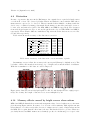
Chapter 6 Spectroscopy pipeline cookbook The spectroscopy pipeline is being developed and maintained by the IRC spectroscopy data reduction team. It is mostly written in IDL, and uses IDL ASTRO library (maintained at the GSFC) among others. Although it is developed under Linux environment, it may be portable to other platform after some modifications (though we have no plan to increase the exportable platforms by ourselves). The toolkit also uses the ds9 FITS viewer for reviewing the images, and the xpa package for communication between the ds9 and the IDL main program. The spectroscopy data reduction requires calibration database (FITS images and ascii tables) distributed and updated also by the IRC spectroscopy data reduction team. The database is based on observations of calibration objects and calibration frames taken during PV/DT phase observations, as well as pre-launch calibration experiments in our laboratory. Therefore observers do not have to make their own calibration observations. 6.1 General overview of the pipeline processing The main pipeline processing consists of several well defined steps, which are explained in the following sections. 6.1.1 Dark subtraction Scaled super-dark images are subtracted from the raw data. For the scaling, dark count offset is calculated within the pipeline, by comparing average counts at the slit-mask-covered portion of the pre-dark image, and the corresponding area on the super-dark image. Additionally the average dark counts of the mask-covered portion of each observed sub-frame is measured, except for LG2 for which there is no good dark area on the spectroscopy images for measuring the dark level. The averaged offset is added to (or subtracted from) the super-dark to make the scaled super-dark. 6.1.2 Linearity correction Linearity correction is made following the method adopted for imaging data reduction. 6.1.3 (monochromatic) Flat-fielding In the case of the slit-less spectroscopy, the entire FOV is the aperture for the background sky, but the object image itself is the aperture for the object. This aperture size difference makes difficulties in flat-fielding the slit-less spectroscopy images since, unlike a conventional long-slit spectrograph, a given pixel can be illuminated by background photons with a range of wavelengths within the disperser’s passband, and the mixing fraction of photons of different 83 IRC Data User Manual 84 wavelengths depending on the spatial distributions and spectra of sources. We need 3D flat information (X, Y along space, plus Z along the wavelength) for full flat calibration. However it is impossible to obtain such a detailed flat since there are no good monochromatic flat light nor a series of narrow-band filters covering the passband of the disperser. Because of these difficulties, we will make a flat calibration in two steps, starting with the monochromatic correction. To correct for the pixel-to-pixel variation of the monochromatic response (response or flat that does not depend on wavelength), the whole image is divided by the ’super-flat’ . The super-flats are made by combining a larger number of background spectroscopy images. Note that the background sky image is not flat along Y or the wavelength axis, i.e., there are several spectral features on the ’super-flats’ due to, e.g., contributions of zero-th or higher-order light in cases of grism spectroscopy images. Although the features should be removed to correct for the pixel-to-pixel variation of the response, we first divide the dark-subtracted images by the super-flat with the spectral features. As shown below in equation 6.1.1, this process makes the background flat, facilitating the sky subtraction. Assume that the dark-subtracted images are represented by the following equation: obs = sky × F1 (x, y) × spectral f eature(x, y) + obj(λ) × F2 (x, y, λ) × R(λ) (6.1.1) where F1 (x, y) is the flat in which the background spectral features are not present, F1 (x, y) × spectral f eature(x, y) is the ’super-flat’, F2 (x, y, λ) is the wavelength-sensitive flat (see below for color-term correction), and R(λ) is the spectral response. Since the super-flat is only a function of the position in the detector, this step is called monochromatic flat-fielding. If we divide the observation by the ’super-flat’, we obtain: obs = sky + obj(λ) × F2 (x, y, λ) × R(λ)/[F1 (x, y) × spectral f eature(x, y)] 6.1.4 (6.1.2) Background subtraction (from individual sub-frames) After monochromatic flat-fielding, background should be flat over the aperture. However, in real data, this is not the case for most of the cases. For NP, NG, and SG1 , outlier-tolerant loworder polynomial surface fitting is performed for each sub-frame, and is subtracted off from the flat-fielded images. For SG2 and LG2, background suffers from so-called ’stray light’ (of the earth shine) contamination, and the flat-fielded images are much more structured. To make good sky subtraction, median running-box filter is applied to estimate the local sky, and is subtracted off from the ’stray light-covered’ background. Such background should be removed from individual sub-frames, since contribution of the ’earth shine’ depends on telescope pointing angle from the earth direction, and amount of the stray light changes within a single pointing maneuver (or within a single AOT operation). In the first pass of the processing within the pipeline, source masking will not be applied in determining the background, because no source position information is available at the stage. In the second pass, after processing through section 6.1.9 once, the background is measured again while considering the source masks. The image obtained after background subtraction has the following expression: obs = obj(λ) × F2 (x, y, λ) × R(λ)/[F1 (x, y) × spectral f eature(x, y)] 6.1.5 (6.1.3) Image screening Some sub-frames may be severely damaged by cosmic-ray shower, a satellite passing in front of the telescope, etc. If this is the case, one can interactively set the flag, by using ds9, for any sub-frames to be discarded in the following processes. Version 1.3 (September 13, 2007) 6.1.6 85 Image registration (among sub-frames) Relative image shift due to satellite attitude drift among spectroscopy sub-frames is measured by means of cross-correlation technique. This can be made only with NP and NG due to the number of spectra present in NIR images. For SG1, SG2, and LG2, pixel offsets measured with NP/NG are used for matching, rather than measuring their own shifts, since all cameras take images simultaneously. Similar shift-and-add technique is also needed for the reference sub-frames, except for N3, where there is only a single reference sub-frame. To find the shift values for L18W, we first detect point sources in S9W , measure their positions, and calculate the shift by using the list of target coordinates, and shift both S9W and L18W images. 6.1.7 Imaging stacking After registering all the sub-frames, all the selected (screened) sub-frames are combined to make higher S/N stacked images. For spectroscopy images, a three-sigma clipping averaging method is used. For reference images, a simple median averaging is used due to the small number of sub-frames. 6.1.8 Target detection/position measurement Target positions can be provided by the user in a form of the source table (see below), or automatically computed within the toolkit, using the daofind method for target detection. Even if the target positions are set by users, the toolkit performs re-centering of the source positions by means of Gaussian peak search. (This functionality can be disabled with the command line option.) This process is coupled with the following step (background subtraction). 6.1.9 Background subtraction (from stacked image) Although background subtraction has been already applied before stacking images, we here remove any remaining background. The background subtraction and target detection/position measurement (explained in the previous section) are made iteratively in the following way. First, the target is tentatively detected by the automatic source detection program (not based on the user-supplied source table), and source masks will be created for all detectable sources. Then the background is measured while considering the source masks, and is subtracted off from the original stacked image. The background-subtracted image is used for better source detection/position measurement, and better source masks will be created for better background subtraction. After sources are detected, source masks are created for better background subtraction from individual sub-frames (section 6.1.4) in the second pass of the pipeline processing. 6.1.10 Extracting 2D spectra By using the reference image positions and pre-defined coordinates offsets in the calibration database, rectangle areas around the source spectra are extracted on the spectroscopy images. For NP, spectral distortion (see below) is taken into account along the dispersion direction to find best Y offset when extracting 2D spectra. X-offset adjustment in spectroscopy image extraction In real data, one need to further adjust the offset of the source extraction boxes. One may sometimes find 2D spectra slightly away from the expected position (at the center of the extraction IRC Data User Manual 86 box) along X axis. This kind of shift can not be corrected in the previous image registration processes, and the correction can be made at this stage. The center position of the 2D spectra is measured for each extracted 2D spectra, and calculate the mean X offset from the center of the extraction box. If the pipeline successfully finds the shift value, the shift will be applied in extracting the 2D spectra. However, for some cases where only very faint objects were detected, calculating this additional shift may fail (and no further shift will be applied). Measuring the X offset and making good source masks (as explained in the previous section) are closely related to each other during the pipeline processing. In the first pass of the source detection, automatic source detection sub-program works even if the target table is supplied in the pipeline command line. The X offset is measured with the tentatively detected sources at this stage. In the second pass, measured X offset (as well as Y offset found in adjusting the wavelength zero reference point; see the next section) between spectroscopy and reference images is taken into account in extracting the 2D spectra. Only the sources specified in the source table, or sources detected with the sub-program, will be processed (extracted) in the second pass. This two-stage process ensures good source masking for better sky subtraction and good offset measurement with brighter and larger number of sources, even for the cases in which observer is just interested in small number of faint sources. Measurement of the center position of the 2D spectra can be made easily for NP, NG, and SG1 spectra for which larger number of brighter sources can be detected even at blank sky region. Therefore, the toolkit measures the X offset at NP and NG for correcting both NP and NG, and at SG1 for correcting SG1, SG2, and LG2. Therefore, user must start pipeline processing for NP/NG first, then SG1, and finally SG2 and LG2. See section 6.4.1 for more explanations. 6.1.11 Wavelength calibration In the case of grism spectra, the dispersion equation is almost linear theoretically and a linear equation for expressing the wavelength is assumed. Therefore, once the 2D spectra extraction is made at sufficient accuracy, it is straightforward to make a wavelength calibration. For prism (NP) spectra, since the dispersion equation is highly deviated from the linear one especially at shorter wavelength end, it is better not to transform images to avoid introducing extra uncertainties in the image interpolating/extrapolating processes. Rather, a separate array (whose length is equal to the Y length of the extracted 2D spectra) will be created to store the wavelength values for each Y pixel. One wavelength array is applicable for all the extracted spectra within the FOV. This kind of wavelength array is also used for grism spectra (NG/SG1/SG2/LG2). Finding wavelength zero reference point Some problems arise for accurate wavelength determination. One is the satellite attitude stability problem. If the satellite pointing moves between reference and spectroscopy images, reference image does not provide good wavelength zero reference point any more. NP spectrum (before flux calibration) shows a notable peak around 2.4μm, and there are lots of fairly bright stars with almost identical spectra regardless of the type of stars within a single FOV. Therefore it is possible to find the best offset of the wavelength zero reference point, by measuring the NP peak positions with respect to the spectral template that was taken when satellite attitude stability was good enough, by averaging the offsets measured for many stars. Once the offset is measured, extraction of the 2D spectra is made again, after considering the Y offset (as well as X offset as explained earlier). Zero reference point is much difficult to be found in NG spectra, due to lack of notable spectral features before applying the flux calibration. Therefore, although the toolkit can estimate the Version 1.3 (September 13, 2007) 87 reference point by examining the observed spectroscopy images, it is strongly recommended to check the zero-th order light images for better wavelength calibration accuracy. The chance of detecting zero-th order light image at significant level for SG1, SG2, and LG2 is not so large. Therefore the drift of the wavelength zero reference point is calculated by using the drift measured in NP or NG for MIR-S/L grisms, after correcting the pixel scale difference. Another issue related to measuring the wavelength zero reference point is the finite pixel resolution. Although the source positions can be measured with an accuracy of less than one pixel size unit on the reference image, extraction of the 2D spectroscopy images can only be made on integer pixel number to avoid erroneous image interpolation. This means that as large as ±0.5 pixel error could be introduced in the wavelength calibration process if not corrected, and is not so small comparing with the full length of the dispersed spectroscopy images (∼ 50 pixel). As a first-order correction, we shift both the wavelength array and spectral response curve, both of which should show rather smooth change along Y (or wavelength) axis, and not perform sub-pixel shifting of the images. As a result, since object positions change slightly among different pointing observations, wavelength at the same Y pixel of the extracted 2D spectra (or the wavelength array) also changes with different pointing observations. 6.1.12 Flat color-term correction The presence of significant color variation in the flat images can be found in the ratio images of the broad-band flats (e.g., S7 flat / S15 flat). Therefore, although monochromatic flat-fielding can flat the background, the object spectrum is affected by the color term of the sensitivity. The correction for this could be done after extracting the 2D spectra for each target and applying the wavelength calibration. However, since we have only two broad-band filters for MIR-S/MIR-L (S7 and S15 for MIR-S, and L15 and L24 for MIR-L) and three for NIR (N2, N3, and N4), we can derive only global trends of wavelength-dependence of the flats. (Note that the wide-band filters, S9W and L18W, are not suitable for deriving the color dependence of the flat within the spectral coverage of the channel). Two broad-band flat images are interpolated to estimate the flats for a given wavelength in the following way: F2 (x, y, λ) = [F (x, y, λ2 ) − F (x, y, λ1 )]/(λ2 − λ1 ) × (λ − λ1 ) + F (x, y, λ1 ) (6.1.4) where λ2 and λ1 are effective wavelength for broad-band filters. The equation 6.1.3 leads to: obs = obj(λ) × R(λ) × F2 (x, y, λ)/[spectral f eature(x, y) × F1 (x, y, λ)] (6.1.5) and, the color term is expressed as F2 (x, y, λ) = spectral f eature(x, y) × F1 (x, y) F (x,y,λ2 )−F (x,y,λ1 ) λ2 −λ1 × (λ − λ1 ) + F (x, y, λ1 ) spectral f eature(x, y) × F1 (x, y) (6.1.6) Therefore the color-term correction is calculated by two broad-band super-flats and one spectroscopy super-flat. Note that the product F1 (x, y) × spectral f eature(x, y) always appears together, i.e., we do not have to separate spectral f eature term from the ’super-flat’. After the color-term correction the image is as follows: obs = obj(λ) × R(λ) (6.1.7) For the NG spectra with the point source aperture (Np), flat-fielding will be made in a similar way to the slit spectroscopy of diffuse sources, since the aperture size is much smaller than the IRC Data User Manual 88 size of dispersed spectroscopy images. For spectroscopy with NG at Np and other slit spectroscopy data calibration, the super-flat is normalized to be unity at each wavelength (or Y) pixel, and there are no spectral features in the flats. On the other hand, NG spectra at Nc will be reduced in the same way as for other slit-less spectroscopy. 6.1.13 (local) Background subtraction (from extracted 2D spectra) Although the background has been subtracted and it should be close to zero at this stage, we here locally subtract any remaining background on the extracted 2D spectroscopy images. Here we consider source masks for better determination of the local background. Background is measured and subtracted off by assuming constant background value across the images for all dispersers. 6.1.14 Spectral tilt correction Although we do not reform image ’shape’ along wavelength direction during the course of wavelength calibration because of simple linear grism dispersion, we do reform along X (or space) direction to correct spectral tilt. The tilt occurs due to misalignment of grism insertion direction with respect to chip orientation. The tilt is notably seen in NG image in which as large as ΔX 2 pixel shift is observed over the longer dispersed image length (ΔY 250 pixel). Similar tilt is also observed for other prism/grisms (NP, SG1, SG2, and LG2), although the tilt looks very small due to short dispersed image length. However, tilt correction will be made for spectra of all types of dispersers. 6.1.15 Spectral response calibration The spectral response calibration R(λ) depends exclusively on the wavelength. Therefore the response calibration table is a 1D vector (lambda vs. ADU/s/mJy). This means that response variations of individual pixels have been removed beforehand by flat-fielding processes. Being different from spatial flat correction, spectral response varies significantly along wavelength due to change in quantum efficiency of chip and change in optical transmission along the camera optical trains, including the disperser. The observed wavelength-calibrated 1D spectrum in ADU is just divided by the spectral response table. Since the wavelength for a given pixel in the observed spectrum is slightly different from that in the response table, simple interpolation will be performed to match the wavelength of the observed wavelength-calibrated spectrum with that in the response table. 6.1.16 Notes on slit spectroscopy The same pipeline can be used for both slit-less and slit spectroscopy data reduction. Although the reduction of the slit spectroscopy data can be made in a similar way as for the slit-less spectroscopy data, there are some differences in some processing steps between the two. Here we summarize these differences. • The slit spectroscopy flat-fielding consists of a normalized feature-less flat image. Therefore no color-term correction is necessary. • Background subtraction is made on extracted 2D spectra in the case of point sources slit spectroscopy (Np), after stacking sub-frames. If dealing with slit spectroscopy for diffuse sources, the background subtraction is not performed since entire slit is expected to be filled with the object that is diffuse and there is no pure background area in the image. Version 1.3 (September 13, 2007) 89 • Shift-and-add feature of sub-frames will be disabled. • In the wavelength calibration, measurement of the reference image positions will not be made, and pre-defined slit positions will be used as a wavelength zero reference point. 6.2 How to install and to set-up the IRC spectroscopy pipeline So far only Linux environment has been tested for running the package. However, the package seems to run on the MAC OS-X environment, though it is not officially supported. • Ask you local computer administrator for the IDL installation. There are no special requests in the IDL installation. • Ask you local computer administrator for the ds9/xpa installation. There are no special requests in the ds9/xpa installation. • Get the irc specred package from the AKARI Observer’s web site (see section 1.2). Extract and store it under your favorite directory. • Set the following environment variables in your command-line shell. Below is an example for csh: setenv setenv setenv setenv setenv setenv IRC IRC IRC IRC IRC IDL SPECRED ROOT <somewhere> SPECRED LIB ${IRC SPECRED ROOT}/LIB/ SPECRED HOME ${IRC SPECRED ROOT}/ASTRO-F/ SPECRED CALIBDIR ${IRC SPECRED HOME}/IRC SPECRED/CALIBDIR/ SPECRED DATADIR <anotherwhere> PATH +<IDL system path>:+${IRC SPECRED HOME}:+${IRC SPECRED LIB} IRC SPECRED ROOT, IRC SPECRED DATADIR, and IDL PATH, have to be modified by substituting <somewhere>, <anotherwhere>, and <IDL system path>, according to your local system settings 1 . 6.2.1 Data preparation As explained in Chapter 3, when de-packing the data from the archive under IRC SPECRED DATADIR, the raw data will be stored in IRC SPECRED DATADIR/<targetid>.<targetsubid>/rawdata. IRC SPECRED DATADIR, <targetid>, and <targetsubid> will be used in the command line of the pipeline command. All the reduced data and related information will be stored in a separate directory called <root dir>/<targetid>.<targetsubid>/irc specred out. When the directory is missing, the toolkit will create it. 6.3 Calibration data When de-packing the toolkit, the following calibration directories are created: 1 In the following, contents within the parentheses <something> should be changed according to user’s interests. IRC Data User Manual 90 6.3.1 Calibration files • ${IRC SPECRED CALIBDIR}/DARK contains dark images with high S/N, combined with precompiled dark images, which can be applied for all the observations, after applying a small correction in the count offset. There are several ’super-darks’ for NIR/MIR-S/MIR-L (as specified in the following list files). – DARK/DARK NIR long.lst, DARK/DARK NIR short.lst – DARK/DARK MIRS long.lst, DARK/DARK MIRS short.lst – DARK/DARK MIRL long.lst, DARK/DARK MIRL short.lst • ${IRC SPECRED CALIBDIR}/FLAT contains two types of flats: super-flats for spectroscopy and reference images. These super-flats are made by combining a large number of blank sky images: For slit-less spectroscopy: – FLAT/SPEC2DFLAT NP.lst – FLAT/SPEC2DFLAT NG.lst – FLAT/SPEC2DFLAT SG1.lst – FLAT/SPEC2DFLAT SG2.lst – FLAT/SPEC2DFLAT LG2.lst For slit spectroscopy: – FLAT/SPEC2DFLAT NP slit.lst For reference images and color-term correction of the flats: – FLAT/IMAG2DFLAT N3.lst – FLAT/IMAG2DFLAT N4.lst – FLAT/IMAG2DFLAT S7.lst – FLAT/IMAG2DFLAT S9W.lst – FLAT/IMAG2DFLAT S11.lst – FLAT/IMAG2DFLAT L15.lst – FLAT/IMAG2DFLAT L18W.lst – FLAT/IMAG2DFLAT L24.lst • ${IRC SPECRED CALIBDIR}/MASK contains images of known bad pixels (hot pixels, cold pixels, etc.). Masked area are marked by NaN (Not a Number) in the mask images. – MASK/SLITMASK NIR.lst – MASK/SLITMASK MIRS.lst – MASK/SLITMASK MIRL.lst – MASK/OUTLIERMASK NIR.lst – MASK/OUTLIERMASK MIRS.lst – MASK/OUTLIERMASK MIRL.lst Version 1.3 (September 13, 2007) 91 • ${IRC SPECRED CALIBDIR}/COORDOFFSET contains a table of coordinate offsets in pixels (dX, dY) used to extract spectroscopy images for each object based on target positions on the reference image for all dispersers. The table also includes sizes of source extraction boxes (ΔX, ΔY) on reference and spectroscopy images, and offsets (dX, dY) for zero-th order light image position. – COORDOFFSET/IRCCOORDOFFSETPAR.dat • ${IRC SPECRED CALIBDIR}/WAVEPAR contains the wavelength calibration tables. For grisms (NG/SG1/SG2/LG2), wavelength (μm) is expressed by 1st order polynomial (linear) equation, and parameters are (1) dispersion (dλ/dY), (2) wavelength at origin (λ0 ), and (3) position of the origin (Y0 ). In the toolkit, position of the origin is fixed to the center of the extracted spectroscopy image. Therefore, only dispersion and wavelength at origin are set in the calibration database files. The parameters can be applied for all the spectra within the FOV (i.e., the parameters are constant across the FOV). Effective wavelength ranges (there are two kinds of range definitions: ’sensitive’ and ’reliable’ ranges) for each disperser are also set in the table. For NP, pixel positions for given λ is expressed in 2nd-order polynomial equation, and there are three parameters (0th, 1st, and 2nd-order coefficients). Note that, for data analysis convenience, the equation is in pixel=function(λ) form, being in inverse form for the grisms. Effective wavelength ranges are also set in the table. Only for NP, significant spectroscopy distortion exists, i.e., reference positions on the spectroscopy images can not be represented by a constant pixel shift (dX, dY) from reference image positions. The deviation of pixel shift along wavelength axis (or Y axis) from the case of constant pixel shift is expressed in 3rd-order polynomial equation of reference position (dYdistortion =function(Xref , Yref )). Polynomial coefficients are tabulated in a separate ascii table, and is stored under the same directory. Note that spectroscopy distortion along X (dXdistortion ) is not so significant, and constant pixel shift works rather well for NP, as in the same way for NG/SG1/SG2/LG2. – WAVEPAR/IRCWAVEPAR COMMON.dat – WAVEPAR/IRCWAVEPAR NP.dat – WAVEPAR/IRCWAVEPAR NG.dat – WAVEPAR/IRCWAVEPAR SG1.dat – WAVEPAR/IRCWAVEPAR SG2.dat – WAVEPAR/IRCWAVEPAR LG2.dat – IRCSPECBOXDYPAR NP.dat • ${IRC SPECRED CALIBDIR}/RESPONSE contains ascii files tabulating λ vs. ADU/long exposure time in seconds/mJy for each disperser. There are five such tables (NP/NG/SG1/SG2/LG2). The spectral response is measured by observing flux standard stars with known flux energy distribution. This directory also contains a NP template spectrum (wavelength-calibrated spectrum, before calibrating spectral response) that will be used to find relative image shift along dispersion direction (or Y) between spectroscopy and reference images. – RESPONSE/RESPONSE NP.lst – RESPONSE/RESPONSE NG.lst – RESPONSE/RESPONSE SG1.lst IRC Data User Manual 92 – RESPONSE/RESPONSE SG2.lst – RESPONSE/RESPONSE LG2.lst • ${IRC SPECRED CALIBDIR}/DISTPAR contains ascii tables tabulating spectral tilt information of the grism insertion angle. – DISTPAR/IRCDISTPAR NP.dat – DISTPAR/IRCDISTPAR NG.dat – DISTPAR/IRCDISTPAR SG1.dat – DISTPAR/IRCDISTPAR SG2.dat – DISTPAR/IRCDISTPAR LG2.dat • ${IRC SPECRED CALIBDIR}/APCOR contains ascii tables tabulating spectral aperture correction table. – APCOR/APCOR NP.dat – APCOR/APCOR NG.dat – APCOR/APCOR SG1.dat – APCOR/APCOR SG2.dat – APCOR/APCOR LG2.dat 6.4 Running the pipeline 6.4.1 Data reduction order The pipeline has to be run more than once, for NP (AOT0a) or NG (AOT0b) first, then SG1 and SG2, and finally LG2. We need to start processing on shorter wavelength cameras (NIR and MIR-S), where larger number of brighter sources are expected to be observed within the FOV as position reference sources. The information derived there will be used for registering longer wavelength cameras (MIR-S and MIR-L). • to measure relative X and Y shift among spectroscopy sub-frames of NP/NG for registering spectroscopy sub-frames of NP/NG/SG1/SG2/LG2. • to measure relative X and Y shift among reference sub-frames of S9W (with larger number of brighter sources) for registering imaging sub-frames of S9W and L18W. • to measure relative X and Y shift of the spectroscopy image with respect to the reference image of NP or NG for registering reference and spectroscopy images of NP/NG/SG1/SG2/LG2. Therefore the data reduction order should be as follows: • First run: run the pipeline for NP (AOT04a) or NG (AOT04b), without a target table for enabling automatic target detection sub-program. For NG data with point source aperture (Np), one needs to run the pipeline first without /Np spec option For other types of slit spectroscopy, one may skip this run because shiftand-add feature is disabled for this observing mode. Version 1.3 (September 13, 2007) 93 • Second run: run the pipeline for your desired targets. Make target tables for N3, S9W, and L18W on the raw images (at this stage only N3 image has been processed). Run the pipeline again for NP/NG/SG1/SG2/LG2 with target lists. Image shift database created previously with NP/NG will be used for the 2nd run. If your target is compact and bright enough to be detected by the source detection sub-program, you do not have to perform this 2nd run. For the 2nd run, begin processing for NP/NG first, then SG1, and finally LG2. • Third run: run the pipeline again if you want to revise the target table. This is optional. Now you got processed reference images for revising the target tables. Run the pipeline again with the updated target tables to see final results. 6.4.2 Running the pipeline Type the following in the IDL command line (a command in a single line): irc specred, <targetid>, <targetsubid>, <ext source table>, <refimage list>, <specimage list>, <filter spec> Mandatory arguments: • targetid: ID of the pointing observation. The information will be provided with the data distribution. Example: 1331048 • targetsubid: Sub-ID of the pointing observation. The information will be provided with the data distribution. Example: 1 • ext source table: An ascii list describing source position (X, Y) in pixel, or the target table. Example: myobjects.tbl cat myobjects.tbl 100.0 100.0 200.5 200.5 150.0 150.5 This will extract spectra of sources located at (100.0, 100.0), (200.5, 200.5), and (300.0, 300.5) in pixel on the reference image. If ext source table is set to ”” (null string), then the pipeline activates its sub-program for automatic source detection. There are some important tips in preparing the source table: – Coordinates counts from 1, not 0, i.e., coordinates of the lower left corner of the image is (1, 1), not (0, 0). – For NIR the toolkit interprets by default the pixel coordinates as measured in the raw image (before the image rotation). When one measures the source positions in the processed images (after the image rotation), set the /rotated NIR source table option at the pipeline command line. – For MIR-L, one can use Y range of either 257-512 (for images before detaching MIR-S/L) or 1-256 (for images after detaching MIR-S/L) to set Y position of the targets. The pipeline subtracts 256 from the Y input if Y>256. IRC Data User Manual 94 • refimage list: An ascii file listing FITS file names of reference image. Example: N3.lst cat N3.lst F000001 N.fits A default list is provided with the data distribution, and is found in /rawdata directory. • specimage list: an ascii file listing FITS file names of spectroscopy images. Example: NP.lst cat NP.lst F000002 N.fits F000004 N.fits F000006 N.fits A default list is provided with the data distribution, and is found in /rawdata directory. Even if you find some images being damaged severely and you do not want them to be included in the pipeline processing, you must list all the images in the input list. Then you should specify the sub-frames to be removed on ds9 within the pipeline. This is because the file names and their order in the list are used to relate FITS files to the exposure timing along the AOT operation sequence. • filter spec: a string specifying a disperser for the processing. Set one of the following: N3 NP, N3 NG, S9W SG1, S9W SG2, L18W LG2 Options • root dir: a string specifying a directory in which a set of data is located. If set, this overrides the setting found in the environment variable IRC SPECRED DATADIR. Example: root dir=’/DATA/ASTRO-F/IRC/SPEC/’ • /Nh spec, /Ns spec, /Ls spec: flags for slit spectroscopy data reduction. • /Np spec: a flag for Np spectroscopy data reduction. See section of ’notes on slit spectroscopy’ for more information of slit spectroscopy data reduction. • /no tune sourcepos: a flag for disabling source position tuning subprogram within the pipeline. By default, irc specred tries to measure accurate source positions by searching Gaussian peak around the coordinates set in the target table. This flag disables this functionality. • /use short refimage: use a short exposure image to measure source positions. By default, irc specred uses the long exposure frame for measuring source positions in the reference image. With this flag set, the toolkit uses the short exposure frame for measuring the source positions. Note that the data reduction will be made for both short and long exposure frames even with this flag set. This flag could be useful for measuring source positions of bright and saturated objects in the long exposure frame. • savefile: set this option to a named variable that will contain the file name of the IDL save file (section 6.5.5). The simplest way to restore the IDL save file is to run irc specred with the savefile=savefile option, and issue restore,savefile command after irc specred finished and before, e.g., plotting the spectra. Version 1.3 (September 13, 2007) 95 Outputs • Whole image products: – Processed and stacked reference image (and corresponding mask and residual (reference image × mask) images). Dark subtraction, flat-fielding, and background subtraction are made: <targetid>.<targetsubid>.<filter spec>.refimage bg.fits <targetid>.<targetsubid>.<filter spec>.refimage mask.fits <targetid>.<targetsubid>.<filter spec>.residual refimage bg.fits – Processed and stacked spectroscopy image (and corresponding mask and residual (spectroscopy × mask) images). Dark subtraction, flat-fielding, and background subtraction are made: <targetid>.<targetsubid>.<filter spec>.specimage bg.fits <targetid>.<targetsubid>.<filter spec>.specimage mask.fits <targetid>.<targetsubid>.<filter spec>.residual specimage bg.fits These images are in 3D, and third (Z) dimension is for short (Z=0) and long (Z=1) exposure frames. NaN (Not a Number) represents masked pixel/area. • Extracted image products: – Extracted reference images for individual targets (and corresponding mask images): <targetid>.<targetsubid>.<filter spec>.refimage indiv.fits <targetid>.<targetsubid>.<filter spec>.refimage mask indiv.fits – Extracted spectroscopy images for individual targets (and corresponding mask images). There are two kinds of images. One is wavelength calibrated ( WC) image for which flat color-term correction and wavelength calibration were applied. The other are flux calibrated ( FC) images for which flux calibration was applied as well as flat color-term correction and wavelength calibration: <targetid>.<targetsubid>.<filter spec>.specimage wc indiv.fits <targetid>.<targetsubid>.<filter spec>.specimage mask indiv.fits <targetid>.<targetsubid>.<filter spec>.specimage fc indiv.fits Note that our spectral plotting tool (see below) uses WC image as an input, not the FC image, since the tool does on-the-fly flux calibration after considering various plotting conditions/options. Since the default FC images does not care these, we strongly recommend to use our plotting tool to review the spectra. These images are in 3D, and third (Z) dimension is for source id. NaN (Not a Number) represents masked pixel/area. • Others: – Target information table: a table of target information, such as positions (after source position tuning), flux, and size (Gaussian FWHM). IRC Data User Manual 96 <targetid>.<targetsubid>.<filter spec>.target table.tbl Its format is the following: ID, image x, image y, image mask dx, image mask dy, spec x, spec y, spec mask dx, spec mask dy, flux, image FWHM, spec bgnoise ADU, spec x pos,spec x FWHM, bad sourcepos flag – Target table: If the source detection sub-program is used within the pipeline, a target table will be written. The file format is similar to the input target table. When source position tuning option is on, this file contains the updated source coordinates. <targetid>.<targetsubid>.<filter spec>.source table.tbl – IDL save file: The output of the pipeline will be also be stored in the IDL save file, which is basically a dump file of the IDL memory image at the end of the pipeline processing. See also 6.5.5 to see how to work on the save file. <targetid>.<targetsubid>.<filter spec>.IRC SPECRED OUT.sav – Log of the toolkit processing: a copy of the irc specred logger is saved as an ascii file. <targetid>.<targetsubid>.<filter spec>.log – DS9 region files: DS9 region files that have been used to locate targets on reference and spectroscopy images on ds9. <targetid>.<targetsubid>.<filter spec>.refimage.reg <targetid>.<targetsubid>.<filter spec>.specimage.reg The region files and saved FITS images of whole image products can be used to review the targets on ds9 manually. • Pipeline work files: The following files will be created by the pipeline. The files will be overwritten without notice. User are asked not to delete any of these files. – NP SHIFT XY.dat: for registering NP/SG1/SG2/LG2 sub-frames in AOT04a – NG SHIFT XY.dat: for registering NP/SG1/SG2/LG2 sub-frames in AOT04b – S9W SHIFT XY.dat: for registering S9W and L18W sub-frames – NP SPECBOX SHIFT X.dat: for shifting SG2/LG2 along X in AOT04a – NP SPECBOX SHIFT Y.dat: for shifting the wavelength zero-reference point for NP/SG1/SG2/LG2 in AOT04a – NG SPECBOX SHIFT X.dat: for shifting SG2/LG2 along X in AOT04b – NG SPECBOX SHIFT Y.dat: for shifting the wavelength zero-reference points of NG/SG1/SG2/LG2 in AOT04b 6.4.3 Summary of interactive operations within the pipeline Although the pipeline program works as a ’pipeline’ (i.e., without interactive operation by uses), some operations in the irc specred do require interactive operation. Version 1.3 (September 13, 2007) 97 • Removing one or more sub-frames before combining the sub-frames: In some sub-frames, one may find severe damage by cosmic-ray shower, nearby satellite passing in front of the telescope, etc. To check the sub-frames and remove from the sub-frame combination list, all the dark-subtracted/flat-fielded/sky-subtracted sub-frames will be shown on a ds9 for reviewing. To remove some sub-frames, use the ’Frame’ -> ’show/hide frames’ pull-down menu of ds9 to hide the frame(s) you need to remove. The toolkit checks the hidden sub-frames and remove them from the internal sub-frame combination list. • Retrying automatic source detection with modified detection parameters: If you use automatic source detection sub-program within the pipeline, you can retry source detection after tweaking the detection parameters. You will see the reference image on the ds9 with detected sources marked, and you are asked to answer if the detection is satisfactory or not. If you answer no, then another dialog with several detection parameter entries pops up. You can edit the parameters, and press OK to re-find the sources. You can repeat this detection process as many times as you like until you get satisfactory source list. The sub-program uses daofind algorithm. daofind parameters in more detail – threshold: Threshold intensity for a point source - should generally be 3 or 4 sigma above background. – fwhm: FWHM to be used in the convolve filter. – sharplim: 2 element vector giving low and high cutoff for the sharpness statistic (Default: [0.2,1.0] ). Change this default only if the stars have significantly larger or smaller concentration than a Gaussian. – roundlim: 2 element vector giving low and high cutoff for the roundness statistic (Default: [-1.0,1.0] ). Change this default only if the stars are significantly elongated. By default, threshold is three times the measured background noise. When too much or too less sources are found, threshold change would give better results, and one does not have to take care of sharpness/roundness parameters in most cases. 6.4.4 Warning messages of the pipeline Some common and frequently appearing warning messages are listed below. • Warning (irc specred): guments, and try again. Wrong number of arguments! Check the command line ar- • Warning: No <..> was found/set...Stop! Some files that should be provided for the pipeline seem missing. Check if list files are properly set in the command line. This warning will also appear if you run SG1/SG2/LG2 data reduction before performing NP or NG data processing, and some mandatory database files, e.g., describing relative image shifts, are missing. • Warning: Offset search box is too small!: When telescope drifts too much, the image matching sub-program fails to find the best shift values among sub-frames. Normally the sub-program resumes searching the shift with larger search box. This message is not so serious for most cases. IRC Data User Manual 98 • Warning: No data are available for measurement... Returning 0! or Warning: Data seems too noisy (sigma=<sigma>)... Returning 0!: These messages will appear if, e.g., detected sources are too faint and their positions could not be measured with good enough accuracy. Check the source detection parameters for better source detections. This message is not so serious for most cases. • Warning: sigma of specbox Y shift measurement seems too large!: This warning appears when the toolkit fails to measure the relative Y shift of NP spectra with respect to N3 reference image. Check the reference image on ds9 to know if source detection could be made successfully. Sometimes the program might detect only cosmic-ray hits, not stars, if the parameters are not optimized. • Warning: sky level is larger than 1.5 times sky sigma!: After extracting spectroscopy images, remaining sky will be subtracted off locally around the source. If everything works fine, the average of the remaining sky should be very small, and is typically less than 1.5 times sky rms fluctuation. This warning message will appear if sky level is larger than the typical value. When this warning appears, check the ds9 image to see if there remains large scale sky level variation. Presence of such sky often indicates failure in monochromatic flat-fielding and/or global sky subtraction, or any big unexpected debris are found. Note that this warning will not appear for slit spectroscopy (including NG at Np). • Warning: Available sky area is too small!: Due to clouded source masking, remaining sky area is too small for measuring sky. Check the source detection parameters for fewer source detection. This message is not so serious for many cases. • Warning: Cross-correlation peak is weak: The cross-correlation function will be calculated while registering sub-frames and/or short and long exposure frames. The peak value of the cross-correlation function is a good measure of the frame registration. The value is 1 for ideal image matching, and is typically 0.6 or larger for real data with noise, but peak of 0.3 is still good. When this warning appears, check the quality of the registered and stacked images. So far registration of the short exposure frame can not be made with good enough accuracy, and one should ignore this warning for short exposure frames. This message is not so serious for many cases. 6.5 Working on the pipeline output 6.5.1 Displaying the whole images on ds9 Here we explain the region marks on the ds9 that shows processed whole image products, e.e., spectroscopy and reference images before source extraction. In the spectroscopy image side (left), • Blue rectangle shows spectroscopy image extraction area. • Green rectangle shows area reserved for the object (or masked area for other objects). • Red rectangle shows plotting area as defined by the spectral plotting tool. • Yellow circle shows the expected positions of the zero-th order light. In the reference image side (right), marked circles correspond source positions (with diameter of the source FWHM). Version 1.3 (September 13, 2007) 99 • Green circles show sources with good position measurements. • Red circles show sources with less accurate position measurements. Source identification numbers are also indicated by the region marks. For clear view of the image under complicated region marks, check out the ’region’ -> ’show regions’ check box in the ds9 pull-down menu. To display these images manually, issue show aperture on ds9, <image>, (/imag) 2 where <image> could be refimage ff[*,*,1] or specimage bg, etc. on the IDL command line. When /imag option is set, the image is shown on right side of the ds9, with region marks for reference image. The default (no option) is for spectroscopy image. See appendix for more on array name conventions. 6.5.2 Displaying the extracted images on ATV ATV is a general-purpose interactive array image-displaying tool. Array should be in 2D. See ATV web page (http://www.physics.uci.edu/ barth/atv/) for more information on the program 3. Command line syntax: atv,array(,/block) Here are some ATV tips: • To display whole images, use atv,<array>[*,*,1]. 1 means long exposure frame (and 0 for short). Here, <array> should be something like refimage bg or specimage bg. • To display extracted images of your desired source id, use atv,<array>[*,*,source id] Here, <array> should be something like specimage n bg. To check mask area, use atv,<array>[*,*,source id]*mask[*,*,source id] • When color table looks abnormal, type set color at the IDL prompt before launching the atv. 6.5.3 Checking for wavelength zero reference point with the zero-th order light image The toolkit calculates the wavelength zero reference point based primary on positions of the objects on the reference image. It also takes into account a wavelength zero-point drift due to satellite attitude drift, as well as coordinate rounding effect when extracting 2D spectra. In most cases, these methods work well to estimate the wavelength zero reference point with accuracy of 0.5 pixel or less. Since positions of the zero-th order light image are also calculated in the same way as for the wavelength zero reference point, one may check the wavelength zero reference point accuracy by comparing positions of expected zero-th order light image and actually observed ones. Unfortunately, this check can be made only when bright sources with measurable zero-th order light images are observed at some part of the FOV by chance. When the shift is found, use the change wave offset command with the estimated wavelength shift in pixel. The shift is calculated from the current position. This command changes the internal variable that records the wavelength offset, updates an offset database on disk, and 2 Items in parentheses () are optional. In some systems, /block option may be required for interactive operation on the ATV. The conditions for which /block requirement seems to depend on local Linux or X11 system settings. The author does not have any good ideas on the correct usage of this option. 3 IRC Data User Manual 100 re-draws the images on ds9 with updated zero-th order light marks. Repeat this command until you get satisfactory result. Then one can use the spectral plot tool for reviewing spectra with updated wavelength and spectral-response calibration. See below for the plotting tools. Command line syntax: change wave offset,<wave offset>,specimage n sff,source table,specimage n wc, wave array,specimage bg where <wave offset> is a pixel number (e.g., 1.0, 0.5, -0.5) to be shifted. 6.5.4 Spectral plotting tool The toolkit’s spectral plotting tool can handle many IRC-spectroscopy-specific features, and we recommend to use it for creating spectral plots. These are some of the functionalities of the tool: • source masks can be considered. (see also /no mask option) • error bars (statistical plus systematical ones) can be plotted. • wavelength offset (along wavelength or Y axis) due to rounding effect of coordinates when extracting the spectroscopy images is considered. • simple image filters for removing isolated ’spike’ pixels can be applied. • aperture stacking along spatial direction and smoothing along wavelength direction can be applied for higher S/N spectra. • shifting aperture positions along spatial direction (X axis) can be made. Command line syntax (a command in a single line): plot spec with image,wave array,specimage n wc,mask specimage n, source table,<source id> or plot spec with image,wave array,specimage n wc short,mask specimage n, source table,<source id>,/short with the following options: • nsum: Number of pixels along X axis combined for plotting. Default is 3. Larger nsum (wider aperture) collects more photons from the object, but this also collects more background noise. Therefore, the best nsum for highest S/N is typically 2 or 3 for point sources (corresponding typical full-width of image PSF). • smooth: Boxcar smoothing width (in pixel) along wavelength direction. Default is smooth=0 (no smoothing). For spectra with higher S/N without loosing spectral resolution, smooth should be 3 (corresponding typical full-width of image PSF). Larger boxcar smoothing window will loose the spectral resolution. Note that when even number is set in the smooth (e.g., smooth=2), the actual smoothing box size would be smooth+1 (e.g., smooth=3). • /sigma filter: This option enables sigma filter operation (at 3 sigma significance level) over 2D spectra to remove spatially isolated high or low count pixels. Default is off. If you find too narrow emitting/absorbing features in your plots, try this option to see if this is a real feature or not. Note that, if there is a cosmic ray hit at the position in one of the sub-frames, such count should be removed as an outlier while combining sub-frames with sigma-clipping averaging method. However, if there are temporal hot pixels or weaker hot/cold pixels that are not shown in the hot pixel mask database, you will find outliers (hot or cold pixels) even after sub-frame combination. Version 1.3 (September 13, 2007) 101 • space shift: shift of the plot extracting box along X (spatial) axis in pixel. Default is zero. Although the pipeline adjusts the X coordinates of spectrum extraction box by measuring positions of spectra, one may find remaining X offset in some cases. Change this offset to find peak position of the flux. If one changes nsum and space shift, issue the display command to see the modified spectrum extraction boxes graphically on the spectroscopy images over the ds9. show aperture on ds9,specimage bg,source table, space shift=<space shift>,nsum=<nsum> (a command in a single line) • /no mask: by default, plots are shown after applying spectral overlapping masks by nearby sources. The /no mask option disables this masking functionality and plot spectra regardless of the possible source overlapping. Since masks are created without examining the source brightness and/or spectral shape (e.g., line emitters, continuum emitters with break, etc.), one may often find the situation where no significant change in plots is found when comparing plots with and without the masking. If this is the case, you can just disable the masking by setting /no mask option. • ps, png, ascii: Plots will be recorded on the files, not on the IDL plot window. – ps=<filename> creates a postscript file (filename.ps) of the plot in the working output directory (under /irc specred out). – png=<filename> creates a png image (filename.png) of the plot in the working output directory. – ascii=<filename> creates an ascii file (λ vs flux and flux errors) (filename.spc) of the plot in the working output directory. User may use gnuplot program to review the ascii output, with the command of plot ’filename.spc’ with yerrorbar. • /with image, tvbottom=<tvbottom>, tvtop=<tvtop>: The 2D image will be shown on TV (an IDL graphic window) below the spectrum plot. Extraction box for plotting 1D spectrum is overlaid. The default is with image=0 (i.e., no TV display). The top and bottom ADU counts for displaying image can be specified with tvtop and tvbottom. These options are active only when /with image is set. • /diffuse: For slit spectroscopy data, spectra will be shown in units of MJy/str, rather than mJy with this option. As of 2007 summer, diffuse flux calibration is not yet fully established. • /no aperture correction: Aperture correction for point-like sources will be applied automatically within the plotting tool. The aperture size, set by nsum, is taken into account to find the correction factor. When the /no aperture correction option is set, the correction will be disabled. To perform good aperture correction, the aperture is centered on the source, and nsum should be 3 or more. Note that the aperture can be shifted by space shift parameter. • Other generic plot options useful in the plotting tool: The plotting tool accepts any kind of IDL-generic plot options for spectral plotting. See plot manual in the IDL documents for full information. Following are some frequently used options. IRC Data User Manual 102 – xrange: plot range along the X (wavelength) axis. By default, plots are shown within the wavelength range set in the wavelength calibration database file along the X axis. If set explicitly in the plotting tool command line, the default settings will be overridden. – yrange: plot range along the Y (flux) axis. By default, plots are shown in auto-scale mode along Y. One can limit/fix the plot range by setting yrange. – xlog, ylog: plotting in log scale along x or y. 6.5.5 Working on saved data All the processed data are saved as an IDL save file, as well as FITS output files. The IDL save file is actually a dump record of the IDL memory image at the end of the data processing. Therefore, one can recall the pipeline results by simply issuing the following command: restore,<savefile>. Here the <savefile> is a string of the save file name. To recall other save file image, issue .reset session first to clear the current IDL memory contents, and then issue another restore command with another save file name. See IDL manual to know more on the IDL save file, restore, and .reset session commands. After restoring the IDL memory, one can use, for example, the following irc specred commands to review the results. • show aperture on ds9, specimage bg • show aperture on ds9, refimage bg, /imag • plot spec with image,wave array,specimage n wc,mask specimage n, source table,<source id> 6.6 6.6.1 Appendix Variable name conventions As a general rule, the extension of the IDL variables ( ff, bg, wc, fc) indicates the finally processed calibration status. Examples: • ff means that the data is processed all the way to flat-fielding. • bg means that the data is processed all the way to background subtraction, i.e., flat-fielded and background subtracted. • wc means that the data is processed all the way to wavelength calibration, i.e., flat-fielded, background subtracted, and wavelength calibrated. • fc means that the data is processed all the way to flux calibration, i.e., flat-fielded, background subtracted, color-term corrected, wavelength calibrated, and flux calibrated. Whole image products: ff and bg are in 3D format (X, Y, short/long ID). Short exposure frame is in Z=0, and long exposure frame is in Z=1. Extracted image products: n images are in 3D. The third dimension is for indicating the source id. They are indicated by n extension of the variable names. The following extensions refer to different processing stages: • n bg: background subtracted on extracted images. • n wc: wavelength calibrated, after color-term corrected, residual background subtracted. Version 1.3 (September 13, 2007) 103 • n fc: flux calibrated, after color-term corrected, residual background subtracted, and wavelength calibrated. Finally, these are the most frequently referred arrays: • refimage bg: Flat-fielded, background-subtracted whole reference image in 3D (X, Y, short/long ID) • specimage bg: Flat-field, background-subtracted whole spectroscopy image in 3D (X, Y, short/long ID) • specimage n wc: Wavelength calibrated extracted 2D spectra in 3D (X, Y, source id) • specimage n fc: flux calibrated extracted 2D spectra in 3D (X, Y, source id) 6.7 Frequently Asked Questions and Troubleshooting 1. Q: Two kinds of flats exist in the spectroscopy data reduction, the imaging flats and the wavelength dependence flats. How should we consider these flats ? A: The IRC slitless spectroscopy differs from more standard slit spectroscopy in that in the latter case, the pixel position and the wavelength correspond on a one-to-one basis. The IRC spectroscopy does not follow this relation and needs to be applied in three steps: • Many spectroscopic flats have been combined to form a super-flat which can be used to remove the pixel to pixel variation of the monochromatic response of the detector. • After subtracting the background, extracting the sources and performing the wavelength calibration, the wavelength flat can be used. The wavelength dependency of the flats is due to the same mechanism to that of imaging mode, and is corrected by interpolating/extrapolating the imaging superflat taken with two different filters for every pixel and the wavelength (colour correction). • Finally, the spectral response specific to the spectroscopic mode observation is corrected by the spectral response function obtained from the observations of standard stars. More detailed explanations can be found in the IDUM. 2. Q: When extracting the spectrum, can the usage of the masks can be avoided? A: The /no mask option is especially relevant in spectral images where the source of interest is much brighter than the others. Results can be compared with and without the /no mask option. 3. Q: What can be done if the spacecraft attitude shifts after the reference frames have been taken? A: The effect will be apparent in the wavelength calibration. For NP only, the signal at the peak of the RSF is used to correct the wavelength reference by default. The result will be inserted into the log file which will be further utilized to correct the drift in SG1/2 and LG2. A shift of more than 1-2 pixels can happen. The actual correction is made by shifting the wavelength array rather than the image array. The SG1/2 and LG2 use the NP/NG as a reference thus one should process the NIR data first. Similarly, for NG in the point source aperture the NG slitless spectroscopy field should be processed first. IRC Data User Manual 104 4. Q: Was the spectral response defined at the centre of the field of view ? A: Basically yes. But the Spectral response at the periphery of the field has been checked for consistency. 5. Q: Does the user have to use a flux calibration aperture ? A: The toolkit can take account of the aperture correction for the slitless spectroscopy, as explained in Section 6 of the IDUM. For the slit spectroscopy, the brightness should be preserved. For the case of small extended sources the user must take special care. 6. Q: Is there any wavelength dependence of the PSF? A: No significant dependence is seen. The PSF in the spectroscopy mode is slightly worse than in the imaging mode, although wavelength dependence of the spectroscopy PSF is not clearly seen.