1
BIOE 504, Fall 2009 41 Problems for Chapter 1 1. (a) Compute mathematically the autocorrelation function, φgg (τ ), for g(t) = exp(−t2 /2σ 2 ). (b) Plot g(t) and φ(τ ) on top of each other using Matlab . (c) Compute analytically the full-width-at-half-maximum (FWHM) values for both g(t) and φ(τ ) and find their ratio. Note that FWHM value is the width of the function in time at half of its maximum value. 2. (a) Fig 1.12 (Fig 15) illustrates two rectangular function g1 (t) and g2 (t). Draw by hand the cross correlation function φ12 (τ ). Carefully label all the features in variables as I did below. (b) How does the result from part (a) change if you convolve g1 and g2 ? Figure 15: Illustration of rectangular function from problem 2. 3. [Matlab Exercise.] Use the following code to generate a matrix of 100 waveforms. Call it matrix G, which has dimensions 1001 ×100 as illustrated below. t=0:0.01:10; %sampling interval T=0.01s and duration T0=10s h1=exp(-(t-5).^2/(2*0.07^2)); %narrowband pulse for j=1:100 f= poissrnd(1,size(t)); %Poisson noise is generated here gg=conv(h1,f)*0.01;G(:,j)= abs(gg(501:1501)); %noise blurred by pulse end BIOE 504, Fall 2009 42 G= g[1, 1] g[2, 1] .. . g(1, 2] g(2, 2] .. . ··· ··· .. . g[1001, 1] g(1001, 2] · · · g[1, 100] g[2, 100] .. . g[1001, 100] The first index indicates samples along the time axis, t = nT = n × 0.01 [sec], and the second index indicates a different waveform presumably from another measurement. (a) Create a vector template, call it h(t), consisting of a 1001 point sequence of values that are all 1 except values between 401 ≤ n ≤ 601 (that is, the central 2 s) where the amplitude is 0.5. Multiply the template h(t) by each waveform in matrix G. Here’s something that works for j=1:100 G(:,j) =G(:,j).*h’; %oooh, bad programming practice... end This new G matrix represents a series of 100 measurement waveforms described as noisy narrowband signals with a region between 4 and 6 seconds that has 50% of the amplitude of the surrounding regions. Plot a few waveforms to be sure that you formed them correctly. Now, devise a simple algorithm that finds the location of the low-amplitude region. Use h as a matched filter on the 100 waveforms to locate the positions of the low amplitude regions. Of course, you already know they are all centered at 5 seconds or index number 501. Specifically, your program must correlate the template with each waveform and identify the time of the correlation peak value. To do the correlation, I recommend that you create a circulant matrix H(800, 1001) where each row is a shifted copy of vector h. For example, H=ones(800,1001); for j=1:800 H(j,j:j+200) = 0.2; end To be sure everything smells right, display H using imagesc(H);colormap(gray);axis square just to be sure it has the correct structure. If you understand what I did above, it should be clear that you need to multiply two of the above matrices and you will get a new 800 × 100 matrix (let’s call it X) of un-normalized correlation functions. Find the index corresponding to the peak values for the 100 correlation functions using [C,I] = max(X); Histogram the index values using BIOE 504, Fall 2009 43 hist(I,nbins) where you pick the number of bins that gives a reasonable looking plot. Print out your program code and the histograms. Also display on the plots the mean value and the standard deviation of distribution. (b) Change the amplitude suppressed region of the template to be only 1 second long and repeat part (a). 4. [Matlab Exercise]. Generate a 10 s ramp function given by g(t) = t/10 for 0 ≤ t ≤ 10 s. Compute the Fourier series and FFT up to 5 Hz. Plot the absolute values of both on top of each other, clearly indicating each, and show that they give the same result. 5. Use closed form integration to show o √π F exp(−a x ) = exp(−π 2 u2 /a2 ) a n 2 2 6. Use the result above, change the appropriate variables, and then use the shift theorem for Fourier transforms to find n o 1 exp(−(x − x0 )2 /2σ 2 ) F h(x) where h(x) = √ 2πσ 7. Prove the modulation theorem: n o 1h i F h(x) cos(2πu0 x) = H(u − u0 ) + H(u + u0 ) 2 8. Compute F d rect dt t 2T0 two ways. (a) First graph (by hand, no Matlab ) the rect function and its derivative. Then compute the transform of the result. (b) Now try the approach of applying the derivative theorem and then computing the transform. The two results should be equal and the answer should involve a sine function. Tell me when you use theorems in your solution. 9. Use closed form integration to show that the 2-D Fourier transform of the circular aperture function F2D circ(r/a) = πa2 jinc(aρ) . The shorthand A circ(r/a) just means a circle of radius a where all values inside the circle at r < a equal A and values outside equal zero. The circle is centered on the origin. For this problem, dust off your ability to integrate in polar coordinates. The first thing to consider is transforming the usual rectilinear spatial variables (x, y) and the corresponding frequency variables (u, v) into p polar coordinates to take advantage √ of the 2 2 symmetry. You know how to do this: r = x + y ; θ = arctan(y/x); ρ = u2 + v 2 ; ϕ = arctan(v/u); x = r cos θ; y = r sin θ; u = ρ cos ϕ; v = ρ sin ϕ. BIOE 504, Fall 2009 44 OK, we have our notation. Now you’ll need these facts: Z ∞ Z ∞ Z 2π Z dy dx = dθ −∞ −∞ J0 (a) = Z α 1 2π 0 Z 2π ∞ r dr 0 dθ e−ia cos(θ−ϕ) ; 0 dβ β J0 (β) = α J1 (α) 0 Jn is a Bessel function of the first kind, nth order. Finally, jinc(ρ) , 2J1 (2πρ)/(2πρ). (a) Compute the 2-D transform to obtain the first line above. (b) What special name does this transform (see below) have? Z ∞ G(ρ) = 2π dr r g(r) J0 (2πrρ) 0 4 3.5 3 FID 2.5 2 1.5 1 0.5 0 −0.5 0 5 10 15 20 time (s) Figure 16: Illustration of the free-induction decay signal in problem 10. 10. One particular magnetic resonance (MR) free-induction decay (FID) signal may be expressed as the sum of three exponentially decaying sinusoids plus a constant, " # 3 X −t/τn FID(t) = M0 + Mn e cos(Ωn t) × step(t) , where Ωn = 2πun n=1 BIOE 504, Fall 2009 45 and u is temporal frequency in Hz. a. Plot the function M1 cos(Ω1 t) e−t/τ1 (by hand! no Matlab ) and label the graph to show approximate values for M1 , τ1 and T1 = 2π/Ω1 . b. Perform the integration to find the Fourier transform of FID(t). c. Explain by examining the equation for FID(t) why the transform is complex. d. Find the real part of the result in part (b). e. Now use Matlab and assume M1 = 1, τ1 = 1 s, Ω1 /2π = u1 = 1 Hz; M2 = 0.5, τ2 = 2 s, u2 = 2 Hz; M3 = 0.333, τ2 = 3 s, u3 = 3 Hz. Plot the result from part (d), i.e., ReF FID(t), from 0 ≤ u ≤ 5 Hz using Matlab and carefully label the axes. 11. You borrowed a spectrophotometer (a photometer that measures optical radiation intensity as a function of frequency or wavelength) from the lab next door because it is 10 times faster than the one in your lab. To calibrate it before use, you illuminate its sensor with a 600 nm wavelength (5 ×10¹⁴ Hz) source known to give a Gaussian-shaped spectrum. Expecting to see the smooth spectrum in the figure below left, you are surprised to observer the scalloped spectrum on the right. Let’s see if we can figure out what is wrong with this system. The user’s manual shows that the system uses a mirror to reflect photons f (t) into the sensor. To make it oscillate faster, the manufacturer had to make the mirror lighter, which also allowed some of the incident light to penetrate the mirror and add back into the main signal but with a t0 = 2 fs (femtosecond = 10−15 s) time delay. Therefore f2 is a time shifted copy of f1 except for the lower magnitude, |f2 | = 0.2|f1 |. (a) Ignoring system effects, i.e., g1 (t) = f1 (t), write an expression for net output g(t) in terms of f1 (t) and f2 (t). See the figure below. (b) Calculate analytically the power spectrum (squared magnitude of the Fourier transform, |G(u)|2 ) using the information above. Plot your final answer and show that you obtain the scalloped spectrum shown in Fig 1.12 (Fig 17). 12. In Example 1.9, we somehow made measurements without the problem of noise. Repeat the exercise in the example but add noise using the Poisson random number generator f=A*poissrnd(L,size(t)); The constants A and L are the amplitude and variance of the noise added. Play with those parameters and give me an example where noise changes my conclusions in that Example. Compute the mean-square error, as in the example, to explain how noise affects your fitting strategy. 13. A new flow cytometer was purchased to size microscopic particles suspended in fluids. While calibrating, you observe the calibration signal and a little random noise as expected, but you also observe a cosine wave that you suspect the system is receiving from radiation emitted by fluorescent lights. There is nothing you can do about it today and you need to measure samples, so you make the measurements anyway. Now you must decide if the cosine signal has contaminated your experiment to the point that results are meaningless or if the data can be used. BIOE 504, Fall 2009 46 Figure 17: Spectrophotometer experiment from Problem 11. (a) To isolate the nuisance cosine signal g(t) you flush particle-free fluid through the system. The cosine signal has a frequency of u0 = 60 Hz and an amplitude of A = 10 mV. Compute the frequency spectrum given by the modulus of the Fourier transform, |G(u)|. (b) Assume the desired calibration signal and nuisance cosine signal sum linearly. The calibration signal is C0 −t2 /2σ2 e c(t) = √ 2πσ and therefore its frequency spectrum is |C(u)| = C0 e−2π 2 u2 σ2 . Plot the calibration spectrum along with your result from part (a) for positive frequencies between 0 ≤ u ≤ 5u0 assuming that σ = 3/u0 . State your decision as to whether the cosine signal’s contribution to the frequency spectrum can be ignored if your experimental data have the same bandwidth as the calibration data. 14. There is a common shorthand notation for convolution that reads Z ∞ g(t) = dt′ h(t − t′ ) f (t′ ) = h(t) ∗ f (t) . −∞ BIOE 504, Fall 2009 47 I try to always write the shorthand notation a different way, using [h ∗ f ](t), because of the following situation. You are using an LTI optical system to estimate the concentration of a substance in the blood as a function of time. A light beam is positioned over a vein and the backscattered energy is recorded to give the measurement g(t). The system is defined by its impulse response h(t) and the substance in the blood as f (t). The substance is injected as a bolus so that f (t) looks like a rectangular function immediately after injection but spreads out in the blood stream according to f (at − b), where a and b are constants. This model suggests that the substance is shifted in time b and scaled by the factor a. Therefore our measurements can be expressed using Z g(t) = ∞ −∞ dt′ h(t − t′ ) f (at′ − b) , and so the notation h(t) ∗ f (t) doesn’t make much sense. Beginning with the equation above, derive the Fourier transform G(u) by first replacing h and f by expressions of the inverse transforms and then proceeding. 15. In Section 1.9, we saw that if g(t) = [h ∗ f ](t) then G(u) = H(u)F (u) because of the Fourier convolution theorem. Using similar arguments, show that if G(u) = [H ∗ F ](u) then g(t) = h(t)f (t). 16. The equation for any instrument classified as linear time-invariant can be written in matrix form as g = Hf +e , where f is an N × 1 column vector of values representing the signal input into the instrument, g is the corresponding N × 1 vector of output values, H is the N × N system matrix that describes how input values linearly map into output values, and e is an N ×1 vector of additive noise. (Assume H is circulant and that Hf is a convolution.) We can analyze properties of the instrument from eigenvalues λk of H, H qk = λk qk , where qk is the kth eigenvector of dimension N × 1 that corresponds to λk . Let’s select a specific eigenvector ei2π(0)k/N ei2π(1)k/N 1 i2π(2)k/N qk = √ e , .. N . i2π(N −1)k/N e and create an N × N matrix out of columns√of eigenvectors, Q = [q0 . . . qk . . . qN −1 ]. The elements of the matrix are Qn,k = ei2πnk/N / N . a. Nice properties of Q stem from orthogonality. Show that Q is an orthogonal matrix. b. Use properties of an orthogonal matrix to find an expression for elements of its inverse, Q−1 k,n . BIOE 504, Fall 2009 48 c. We can decompose the system matrix as follows: H = QDQ−1 . Explain how matrix D is related to the eigenvalues of H. d. Begin with the linear systems equation g = Hf + e. Rewrite this equation using the eigen-decomposition of the system matrix given in part c, and multiply the result by Q−1 . e. Express the term Q−1 g from the result of part d as an equation involving a summation over integer n. f. What is another name for the equation that results from part e? What does the integer index k represent? 17. [Matlab Exercise]. Assume we have the simple 2-D object f [n, m] with dimensions 22 × 22 pixels. See the figure on the right below. Here I placed a 12 × 12 square of 1’s in the middle of a field of 0’s. Next to f [n, m], on the left is the 2-D impulse response of the imaging system h[n, m] that also has dimensions 22×22. However, the only nonzero pixels are near the center, where we find a 2 × 2 block of 1’s. Do not use the native Matlab functions xcorr2, conv2, fft2, or ifft2 for this problem until part (c). Figure 18: Figure for Problem 17. a. Reorder f [m, n] into a 484 × 1 vector, f , as illustrated in Fig 12. Also, figure out a way to reorder h[m, n] into a vector that will become the rows of circulant system matrix H. Recall that the task for reordering h[m, n] into rows of H is to find an ordering where multiplication of f by each row of H is equivalent to multiplying the 2-D functions h[m, n] and f [m, n]. Selecting a different row is the same as selecting a different amount of shift for the circular convolution. Once f and H are constructed, then find the 484 × 1 vector g from the product Hf , as in Fig 11c. Reorder the resulting vector to reconstruct its 2-D form, g[m, n], and display the 22 × 22 pixel image. It should resemble f [m, n] but blurry. You might need to trim the result to make it 22 × 22 pixels. Once it all works, use the Matlab functions tic and toc to time the execution. BIOE 504, Fall 2009 49 b. Use the Fourier convolution theorem to achieve the same effect but do not use fft2 or ifft2 to compute transforms. Instead, construct a Q matrix and use matrix methods to complete the forward and inverse transforms. You may need to trim the result to compare with (a). Also time the computation. c. Finally, use conv2 and fft2 to achieve the same results as (a) and (b) above. For each part of this problem, show me the Matlab code, the images and the computation time. d. You’ll find that g[m, n] may not be scaled in amplitude the same as f [m, n], which means somehow your system matrix is amplifying or attenuating your object signal. Any ideas on how to get rid of the annoying scaling? 18. Compute analytically F (u, v) given that f (x, y) = rect((x − x0 )/X0 ) rect((y − y0 )/Y0 ). 19. [Matlab Exercise]. Prove Eq (8) is correct by numerically computing φaf and φf a where a = rect (t − 0.5) and f = (1 − t) step(t) step(1 − t) . 20. [Matlab Exercise]. Follow Example 1.9 but select another input function (make it interesting). Also add a modest amount of noise via n=a*randn(size(function)); where a is the standard deviation of the normal random noise variable. If you’re not sure, try it and plot everything to make sure you follow how this signal-added-to-noise thing works. Give me the same plots I gave in Example 1.9 (don’t bother with plot (a) showing the polynomials.) Finally, look at the appendix and do an SVD analysis on the same data. Comparing and interpret results by discussing how the polynomial-fitting errors compare with the SVD values.