1
Department of Informatics and Media
University of Applied Sciences Brandenburg
A Theoretical & Practical Introduction to
Self Organization using JNNS
Miguel Angel Pérez del Pino
Prologue
Relating to this text
During the last years of my career, the main intention of my work has been to apply
neural networks to several fields of my interest, mainly networking security and
biomedicine. As Dr. Carmen Paz Suárez Araujo’s, from University of Las Palmas de
Gran Canaria (Spain), and Prof. Ingo Boersch’s, from Fachhochschule Brandenburg
(Germany), undergraduate student I have learned how important the neurocomputing is
becoming in nowadays engineering tasks. Through this path, I have gathered a variety
of ideas and problems which I would have appreciated to be written or explicitly
available for my personal reading and further understanding.
The employment of a simulator to develop first stage analysis and to plan further work
is a must in the engineering discipline. My aim in the development of this brief
textbook has been to compose a little, but well condensed manual, where the reader can
get the point of self organized networks, and moreover, of Kohonen Self Organized
Maps, SOM. Using JNNS, the reader will be able to apply the theoretical issues of
Kohonen networks into practical and real development of ideas.
This brief textbook is oriented to those with little experience in self organization and
Kohonen networks, but also to those interested in using and analyzing the deployment
of solutions with the Java Neural Network Simulator, JNNS.
Text Organization
The text is organized as follows:
1. An introductory part, chapter 1, is presented, where it is written the
fundamentals of JNNS, commenting its origin, structure, functionalities, etc.
2. Chapter 2 shows the theoretical issues of Self Organization and Kohonen
Networks, applied directly to JNNS. The different parts and tools involved in
the simulator with these techniques are presented.
3. Chapter 3 presents a set of case studies and exercises to be developed by the
reader, pointing at important aspects of Kohonen SOM networks and the JNNS
simulator.
A Theoretical & Practical Introduction to Self Organization using JNNS
1
Acknowledgements
It is maybe the most difficult paragraph written in all this set of words and sentences
that I have called text. I would like to thank specially Prof. Ingo Boersch and Dr.
Carmen Paz Suárez Araujo for their help and reviews during this long time I have been
composing this document. Their support has been crucial for me to finish it. I would
like to thank Pablo Fernández López, friend and team-mate at COMCIENCIA,
University of Las Palmas d Gran Canaria, for his continuous reviews and contributions.
In the development and writing of this text, I would also like to thank to all those who
have contributed in reading and reviewing the contents, but mainly to Ubay González,
Iván Martín and Javier Somonte.
MIGUEL ANGEL PÉREZ DEL PINO
SEPTEMBER 2005
A Theoretical & Practical Introduction to Self Organization using JNNS
2
Chapter 1
Introduction to the Stuttgart
Java Neural Networks Simulator
1.1. Overview.
SNNS is an Artificial Neural Networks (ANNs; computational models inspired by
biological neural networks) simulator developed by the High Performance Institute of
Parallel and Distributed Systems (IPVR) of the University of Stuttgart in 1989. The aim
of the project was to create a flexible and efficient simulation environment for the
research on the field of ANNs.
It is made up of four main parts: the simulator kernel, the simulator graphical interface,
the background planner/simulator of models, and the ANSI C networks compiler.
SNNS was developed entirely in ANSI C and its graphical interface is based on the
X11R5 and X11R6 libraries. JNNS has been rebuilt using the Java programming
language, although it keeps the original design idea of SNNS and its based on the
original kernel.
There have been implemented different SNNS versions, depending on the architectures
and operating systems they run: Sun SPARC, DECstation 3100 5000, DEC Alpha AXP
3000, 80x86 IBM-PC, IBM RS6000/320 320H 530H, HP 9000/720 730 and SGI
Indigo2.
JavaNNS (referenced as JNNS) is the successor to SNNS. JNNS is based on the SNNS
computing kernel, but has a newly developed graphical user interface written in Java
set on top of it, [JNNS, 2004]. Hence compatibility with SNNS is achieved while
platform-independence is increased. In addition to SNNS features, JNNS offers the
capability of linking HTML browsers* to it. Moreover, JNNS is cross-platform because
of the Java Virtual Machine. It is available for Microsoft Windows, Solaris and Linux.
It will be referred as S/JNNS all the comments which affect both neurosimulators.
However, this practical text will be oriented to using JNNS.
1.2. Terminology employed by S/JNNS.
A neural network is made up of units (main computational element) and weighted links
with orientation that connect these units. Each unit receives weighted information over
the input set links, makes certain calculations and emits a result, which becomes a
weighted input to many other units.
* For accessing manuals or reference course-books directly from the application.
A Theoretical & Practical Introduction to Self Organization using JNNS
3
In SNNS, the information pre-processing made by an unit is based on a stages
computation, using the activation function in the first stage and the output function in
the second stage. The activation function takes the information received by the input
links in a determined moment of time (net input) and makes the calculation the function
has been assigned, obtaining this way the new unit activation state. The output function
takes the new activation state and calculates the unit output. These functions can be
S/JNNS library functions or defined functions in ANSI C which are linked to the
neurosimulator.
Additionally, S/JNNS allows to model dendritical computation, being able to define
functions which make complex calculations with the information received over the
input connections and, afterwards, send this calculation result as input data to the unit.
It must be said that time, in S/JNNS, is a discrete magnitude.
1.3. Neural Units.
In a neural network model, units (Fig.1.) can be separated into:
1. Input Units: Those which directly receive the network input information.
2. Output Units: Those whose returned output are part of the network output.
3. Hidden Units: Those which are neither network input nor output units. They
receive the output of others units as inputs and their outputs become input to
other units.
S/JNNS allows to define other types of units such as dual units and special units. Every
unit has the following attributes in S/JNNS:
1. Number [no]: Identification number of the unit which at the same time indicates
the storage order in the simulator kernel.
2. Name [name]: Name of the unit. It can be defined by the user and should not
contain blank or special characters.
3. Type [io-type, io]: It indicates the type of unit (input, output, hidden, dual,
special, input special, output special, hidden special). Dual ones can be input
and output ones at the same time; special ones can be used in any way and their
associated weights are not adapted in learning processes.
4. Activation [activation]: The unit activation value.
5. Initial Activation [i_act]: The initial unit activation unit. It is established by the
reset operation.
6. Output [output]: Output unit value.
A Theoretical & Practical Introduction to Self Organization using JNNS
4
7. Threshold [bias]: Used by the activation function. It establishes the value
needed to be surpassed for the unit to be activated. Some learning processes
modify this value.
8. Activation Function [actFunc]: It is the function which allows calculating the
new activation state of the unit by means of its inputs, the actual activation state
and the unit threshold. The general activation function expression can be:
a j (t + 1) = f act ( Net j (t ), a j ,ϑ j ) , Eq. 1
Where:
is the activation value for unit j at time t
Net j (t ) is the weighted sum of the inputs of unit j at time t, taking into
account dendritical computation if exists
ϑ j is the threshold of unit j
a j (t )
The default S/JNNS activation function is the logistic function (Act_logistic),
defined by the expression:
a j (t +1) =
1 , Eq. 2
1 + e− x
The new activation at time (t+1) lies in the range [0, 1]. The variable ϑ j is the
threshold of unit j. The net input Net j (t ) is computed with:
Net j (t ) = ∑ wij oi (t ) ,
Eq. 3
i
9. Output Function [outFunc]: The output function computes the output of every unit
from the current activation of this unit. The output function is in most cases the identity
function (Out_Identity):
o j (t ) = f out (a j (t )) ,
Eq. 4
10. Function Type of Unit [f-type]: It indicates the name of a pattern of the unit
which defines some parameters which are wanted to be shared by a big amount
of units.
11. Position: Spatial position expressed by means of spatial coordinates of the unit.
12. Subnet Number [subnet no.]: Every unit belongs to a subnet. The subnet
concept has been defined to make the handle of the models easier.
13. Layer: The networks can be made up of layers. This attribute defines the layer
the unit belongs to.
A Theoretical & Practical Introduction to Self Organization using JNNS
5
14. Functional Unit State [frozen]: This property indicates if the activation and
output functions are frozen, what means that their values are not being modified
during the simulation.
The values associated to the attributes shown above are represented as floats with 9
decimal digits of precision in S/JNNS.
Fig. 1. Example of Multilayered Neural Network.
Units on the left side are input units; units on the centre are hidden units; on the right side, output units.
1.4. Connections (Links).
The information inside the network is sent or transmitted by means of connections
(links) between units. A connection direction shows the transfer direction of the unit
output value, (Fig.1). The unit where the connection starts from is called source unit,
while the unit where the connection ends is called target unit. There can be connections
where the source and the target unit are the same; these are called recurrent
connections. Redundant connections are not allowed.
Each connection has a weight assigned to it, (Fig.2.). The effect of the output of one
unit on the successor unit is defined by this value: if it is negative, then the connection
is inhibitory, if it is positive, the effect is excitatory.
Weights are represented as floats with 9 decimal digits of precision in S/JNNS.
A Theoretical & Practical Introduction to Self Organization using JNNS
6
1.5. Learning Process.
S/JNNS provide two ways of applying modifications to weights:
1. An online learning where modifications take place after the presentation of each
pattern.
2. An offline learning where the sum of all the individual modifications is made
after the complete presentation of a whole cycle of patterns.
Fig. 2. Connections between input units and output units.
It can be seen the associated weight to every connection, expressed as a float value.
An aspect of interest in Artificial Neuronal Networks is the related to the way of fitting
the weights in order to improve the behaviour of the network, on the basis of
approaching better results in the desired problem. Frequently, this modification usually
is governed by Hebb’s rule, which establishes that the magnitude of modification of the
weight associated to the connection between two units must directly be proportional to
the correlation of activities of these units.
The general expression of the rule of Hebb is defined by the expression:
Δwij = g (a j (t ), t j ) ⋅ h(oi (t ), wij ) , Eq. 5
where g(...) and h(…) are arbitrary functions.
The learning procedure in feed-forward neural networks when supervised learning is
used follows the steps below:
A Theoretical & Practical Introduction to Self Organization using JNNS
7
1. An input pattern is presented to the network.
2. This input is propagated following the network topology until the network
output layer is reached (forward propagation phase).
3. It is obtained an output value from the network and it is compared to the wished
output value, computing a certain error function.
4. This error function is propagated in reverse order to the network topology,
modifying the value of weights in the corresponding way (backward
propagation).
5. It is repeated steps 1, 2, 3, 4 until the error value reaches the wished minimum
value.
In case of unsupervised learning use, there is no separation of the training set into
input and output pairs. A training cycle follows as below:
1. A vector is applied to the visible nodes or to the input nodes if competitive
learning.
2. A winner unit is established.
3. Weight changes are made according to some prescription.
The disappearance of the external supervision is the reason of the “unsupervised” name.
1.6. Updating Process.
The update order of activation values of units is defined by means of the update mode.
SNNS implements five update modes for general use [SNNS, 1994]:
1. Synchronous: Units calculate their activation value all at the same time;
afterwards, units calculate their output value again simultaneously. Everything
is made in a single step.
2. Random Permutations: Units calculate their activation and output values in
sequential form. The order is random and each unit is visited exactly once in
each step.
3. Random: The order is defined on random way, without assuring that all the units
are visited in each step.
4. Serial: Units calculate their activation and output values in sequential form,
being established the order by the unit identification number (no.).
5. Topological: The kernel sorts the units following their topological order (natural
propagation of information from inputs to outputs).
Additionally, other specific update ways of special models of networks exist.
A Theoretical & Practical Introduction to Self Organization using JNNS
8
1.7. Interacting with JNNS.
To make use of JNNS, the computer needs to have Java Run Environment or JDK
(which contains it) installed. JNNS has been tested to work with Java 1.3. Previous
version 1.2 should also work. To install JNNS, it is just necessary to follow the
instructions packed in the compressed file distributed by the University of Tübingen,
[JNNS, 2004].
Once the neurosimulator has been run, the main screen is opened. JNNS is based on a
multiple document interface (MDI); that is to say, multiple windows will be at the
user’s disposal. The main toolbar reflects common menus. An empty neural network
model is initialized by default, (Fig.3).
Fig. 3. JNNS main screen once started up.
S/JNNS defines 3 main types of file extensions:
1. Network Files: Defined by a ‘.net’ extension. They contain the neural network
model structure; that is: network name, source files, number of units, number
of connections, the learning and update functions employed, and all the
weights involved.
2. Pattern Files: Defined by a ‘.pat’ extension. They contain the pattern set
structure; that is: number of patterns compounding the data set, number of
input units in the neural network input layer and, sequentially, all the patterns
definitions line by line.
3. Configuration Files: Defined by a ‘.cfg’ extension. They contain specific data
of interest about the software configuration to be adapted to certain neural
network model or user requirements; that is: learning parameters, updating
parameters, display parameters, etc.
A Theoretical & Practical Introduction to Self Organization using JNNS
9
The creation of a new neural network should start by clicking the FILE/NEW menu
item. This establishes the framework where the neural network model is going to be
built on. It must be reminded the file types detailed above can be generated by using de
FILE/SAVE, FILE/SAVE AS menu items.
The model display can be configured using the VIEW/DISPLAY menu. It helps in the
visualization of the neural network developed, showing and/or hiding certain parameters of
importance in the model analysis. On the other hand, the VIEW menu contains other tools of
interest, such as the ERROR and WEIGHTS analyzers.
In order to incorporate neural units and create layers and to control the learning
parameters, the TOOLS menu must be used. It should be highlighted the menu items
below:
1.
“Create” Menu Item: It allows the construction of the network layers (Fig.4a)
and the interconnections of units, (Fig.4b).
Fig. 4. (a) JNNS Create Layers Window; (b) JNNS Connections Window
2. “Control Panel” Menu Item: It shows the learning and updating control panel,
from where the user can toggle the parameters involved in the network
initialization, training, updating and validation, (Fig.5).
1.8. A practical example.
To interact with the neurosimulator for first time, a neural network example is
presented. This pretends to be an introduction practical case study.
1.8.1. Description.
It is needed to differentiate 4 kinds of screws which pass along a belt and need to be
placed in the correct box. A certain system will be in charge of recognizing and
deciding where to send every screw that goes along the belt.
A Theoretical & Practical Introduction to Self Organization using JNNS
10
Fig. 5. JNNS Control Panel Window
1.8.2. Resolution.
A Kohonen SOM network will be used to carry out this task. The network aims to be
simple and fast enough to handle this job.
1.8.3. Patterns Set Definition.
In such intention, it is necessary to encode every screw by a special feature pattern in
order to be presented to the neural network. The proposed pattern type is based on a
representation using 4-binary digits patterns:
Screw 0
Screw 1
Screw 2
Screw 3
:
:
:
:
0001
0010
0100
1000
Frame.1. Selected encoding.
S/JNNS follows a certain pattern file structure, which must contain:
1. The S/JNNS pattern file header: The first two lines of the file must contain a
reference like the following one, showing the software id and the generation
date:
SNNS pattern definition file V4.2
generated at Mon Apr 25 18:08:50 2005
Both lines are ignored by the simulator at the interpretation time. JNNS accepts
the same pattern file structure as SNNS, due to it is completely based on the
SNNS 4.2 kernel.
2. The number of patterns: It represents the quantity of items compounding the
data set, and so, the number of patterns defined inside the file. It should be
noted after the clause “No. of patterns :”.
3. The number of input units: It represents the dimension of the input data set
space. It should be noted after the clause “No. of input units :”.
A Theoretical & Practical Introduction to Self Organization using JNNS
11
The pattern data set file should look as the one showed in Frame.1. This structure must
be saved in a plaintext file labelled with ‘.pat’ extension. (Note: Using an external text
editor is recommended).
SNNS pattern definition file V4.2
generated at Mon Apr 25 18:08:50 2005
No. of patterns : 4
No. of input units : 4
0001
0010
0100
1000
Frame.2. Screws data encoded patterns.
1.8.4. Neural Network Structure Definition.
Create a new neural network using the FILE/NEW menu item. By using the “Create
Layers” tool, build the following structure:
1. A first layer (Layer 1), with 4 INPUT units, organized vertically in a 1-column.
2. A second layer (Layer 2), compounded by 8 HIDDEN neurons in the X axis and
8 in the Y axis. This means 64 HIDDEN neurons in the second layer. These
neurons should be configured with an “Act_Euclid” activation function to
implement the Euclidean distance in the presented example.
Connect both layers using the “Connections” window, located in the TOOLS main
menu. Select the input units (Layer 1) in the DISPLAY window using the mouse and
define them as “Source Units”. Afterwards, select the hidden units (Layer 2) and define
them as “Destination Units”. The network should appear with connections created
between its layers, (Fig.6).
The pattern file should be loaded using the FILE/OPEN menu item. Select the file
wherever it has been saved in and S/JNNS will interpret it to make it ready to be used
by the neural network.
1.8.5. Training Process.
Once these tasks have been accomplished, both the neural network structure and the
pattern set which defines the input space are defined. The “Control Panel” (CP),
located in the TOOLS menu should be opened. The CP window is made up of 6 tabs,
(Fig. 7):
A Theoretical & Practical Introduction to Self Organization using JNNS
12
1. Initializing Tab: It contains the initialization function and its parameters. For the
example proposed, “Self-Organizing Maps, ver.3.2” should be used. The min
value should be adjusted to “-1” and the max one to “1”.
2. Updating Tab: It contains the updating function and its parameters. For the
example proposed, “Kohonen Order” should be used.
Fig. 6. Neural network example presented.
3. Learning Tab: It contains the learning algorithm and its parameters. In the
example proposed, the following parameters should be adjusted:
-
Learning Function:
Parameter h(0):
Parameter r(0):
Parameter αH:
Parameter αR:
Parameter h:
Cycles:
Steps:
Select “Kohonen”.
1.0
4.0
0.98
0.98
8
1000
1
4. Pruning Tab: It contains special features for algorithms with pruning capability.
5. Patterns Tab: It contains the definitions of Training Set, Validation Set, and the
Remapping Function, if used. Both Sets should point to the main pattern set
loaded in section 1.6.1 – the name of the loaded file should be seen.
6. Sub-patterns Tab: It contains definitions of main pattern-set subsets.
Once the conditions have been set, the neural network weights should be initiated.
Pressing the “Init” button at the Learning tab, this action will be carried out.
Afterwards, press the “Learn All” button to present all the patterns in the pattern file to
the network sequentially over 100 cycles. When the training process is finished, it
should be opened the Updating Tab. In the bottom-right corner, it can be shown each
pattern individually to the network to test its results.
A Theoretical & Practical Introduction to Self Organization using JNNS
13
Fig. 7. Learning Tab at Control Panel Window.
The results of the testing process can be seen in the above figures (Fig. 8a, 8b, 8c, 8d).
Each pattern presentation shows special network behaviour, reacting in different way to
every screw pattern. Green areas show high activation neuron zones, while blue ones
mean lower or no activation.
Fig. 8. (a) Response to Screw 0 Pattern Presentation; (b) Response to Screw 1 Pattern Presentation;
(c) Response to Screw 2 Pattern Presentation; (d) Response to Screw 3 Pattern Presentation
The network has learnt to recognize 4 kinds of screws (0:a; 1:b; 2:c; 3:d).
1.9. Remarks.
It has been briefly presented the JNNS neurosimulator structure and interface. A real
example of classification has also been shown. The main bases of JNNS have been used
A Theoretical & Practical Introduction to Self Organization using JNNS
14
to create and train the neural network proposed, so that he reader gets a general
overview of the software.
In the next chapter, the mathematical and algorithmic framework where Kohonen Self
Organizing Networks are defined will be presented in depth.
A Theoretical & Practical Introduction to Self Organization using JNNS
15
Chapter 2
Self Organization &
Unsupervised Learning
2.1. Introduction.
Self Organizing Systems (SOS) are those which have processes that allow
automatically the internal organization to grow without being guided or controlled by
any external source. SOS usually show emergent properties which allow, starting from
simple rules, to obtain complex structures. Self organizing concept is a basis in the
description of biological systems, from sub-cellular level to ecosystem level. On the
other hand, areas such as cybernetics, cellular automata, random graphs, evolutionary
computing and artificial life, present self organizing features, [García Báez, 2005].
In auto-organized learning, also referenced as non-supervised learning, unlike the
supervised one, there is no need of external helping information, that is to say, there is
no environmental feed-back saying what should be the right outputs for a given input
data. When a self organizing network is used, an input vector is presented at each step.
These vectors constitute the environment of the neural network. Each new input
produces an adaptation of the parameters. Since in these networks learning and
production phases can be overlapped, the representation can be updated continuously,
[Rojas, 1996]. The intention of this kind of learning is to discover significant features,
correlations, or categories in the input data set and to make these discoveries without a
tutor, basing on the observation and redundancy in the information, [Hertz, 1991].
The best-known model of self organizing networks is the topology-preserving map
proposed by Teuvo Kohonen, [Kohonen, 1990]. Kohonen’s model has been built on the
previous Willshaw and Von der Malsburg’s work, [Rojas, 1996].
In this chapter, it is presented a study of SOM Kohonen Networks, their theoretical and
practical aspects and their implementation/simulation under S/JNNS neurosimulator.
2.2. Kohonen Model.
2.2.1. Overview.
Self Organizing Systems make use of local nature rules, that is, the changes suffered by
a neuron’s synaptic weights are influenced by this neuron’s immediate neighbourhood
effect. This has not to be a limitation itself, the global order can arise from local
interactions, Turing said. The neural schemes employed in self-organized learning tend
to follow neurobiological structures much more extensively than the supervised ones.
A Theoretical & Practical Introduction to Self Organization using JNNS
16
However, non-supervised learning can just be useful when there is redundancy in the
input data set, in such a way that redundancy is said to generate knowledge, [García
Báez, 2005].
Kohonen’s model has a biological and mathematical background. It works with
elements very similar to other researcher’s proposals. The relevant issue of this model
is the definition of the neighbourhood of a computing unit. Kohonen’s networks are
arrangements of computing nodes in one, two or multidimensional lattices, [Kohonen,
1990][Rojas, 1996]. Other researchers have also proposed connections of this kind: von
der Malsburg in his self-organizing models [Malsburg, 1973], Fukushima in his
Cognitron and Neocognitron models [Fukushima, 1975][Fukushima, 1980], always
following presented schemes referring to brain structures, [Grossberg, 1976][Kohonen,
1982], [Rumelhart, 1985].
Fig. 9. Kohonen’s Network Bi-Dimensional Topology
This neural network structure is usually made up of an input layer which is connected
feed-forward all-to-all to a bi-dimensional lattice-shape layer; so that it presents a
totally connected or complete topology, (Fig.9). The units located in the bi-dimensional
layer have lateral connections (interactions) to several neighbour units. This grid of
computing elements allows to identify a unit’s immediate neighbours.
It is considered to be important due to during the learning and updating processes the
weights of the unit and their neighbours’ ones are adapted. There is a neighbouring
relationship between the involved units, being this relationship defined by any
geometrical shape (i.e. squared, hexagonal). The objective is that neighbouring neurons
learn to react to similar related signals.
2.2.2. Learning Algorithm.
The objective of Kohonen’s algorithm is the specialization of every unit on different
regions of the input space; that is to say, when an input from such a region is fed into
the network, the corresponding (specialized) unit should compute the maximum
excitation.
A Theoretical & Practical Introduction to Self Organization using JNNS
17
A Kohonen unit usually computes the Euclidean distance between a certain input
pattern x and its weight vector w. Nevertheless, this is not the only expression that can
be used; other similarity-dissimilarity metric measures can be employed (i.e. scalar
product, in which case the bigger the distance, the better the network adjusting),
[García Báez, 2005].
Kohonen’s algorithm uses a neighbourhood function, N, whose value Nc(l) represents
the strength of the coupling between unit c and unit l during the training process. The
winner unit and the ones located topologically near to the winner will learn something
about the input vector x, increasing the similarity or dissimilarity with the input vector.
Fig. 10. Squared and Hexagonal neighbourhoods with 0, 1, 2 size values.
The learning algorithm for Kohonen networks is shown below:
1. The n-dimensional weight vectors, w1, w2, w3 …, wm, of the m computing units are
selected at random. Different algorithms for initialization are presented in section
2.3.
2. A radius r, a learning constant η (which controls the magnitude of weight updates)
and a neighbourhood function Nc(l) must be selected. A neighbourhood functions
analysis will be undertaken in section 2.2.3.
3. Present a selected input vector x to the network.
4. The unit k with the maximum excitation is chosen (that one whose distance between
x and wi is minimal; i = {1, 2, …, m}).
5. The weights are adapted using the neighbourhood function and the update rule.
The repetition of this algorithmic process over the time is expected to generate a global
sorting independently from the initial weight values (which are usually randomly set).
However, it is important the order in which the input vectors have been presented to the
network.
The radius of the neighbourhood is reduced according to a so-called schedule. The
result is the adaptation of the maximum excitation neuron and its neighbours. During
the training process, both the size of the neighbourhood and the value of Nc(l) decrease
gradually, being the influence of each unit upon its neighbours reduced. The value of
the learning constant is also gradually decreased. The effect of the selected scheduling
A Theoretical & Practical Introduction to Self Organization using JNNS
18
on the network is the production of larger corrections at the beginning than at the end of
the training process, [Rojas, 1996].
The SOM learning process is competitive, that is to say, based on the existence of a
winner unit that is the best fitting the input vector (this is the one with less Euclidean
distance or the one with higher scalar product value).
2.2.3. Neighbourhood Effects.
The neighbourhood function Nc(l) is a function expressing the neighbourhood, centred
on c, between the winner unit c and any other unit l. As commented in section 2.2.1, the
main feature of the neighbourhood function is that it decreases as effect of the increase
of distance from the winner unit and as training time passes. The Nc(l) function graph in
relation to the distance between l and c in the SOM layer in a determined instance of
time is used to be Rectangular, Mexican Hat or Gaussian shaped, (Fig.11).
There must also be considered the weight vectors initial values; there are usually
employed little random values. Not considering it, added to the imposed restrictions by
the neighbourhood function, can result in the appearance of an undetermined number of
so-called dead units (units that are never winner to any of the input patterns), [García
Báez, 2005][Rojas, 1996].
Fig. 11. Different neighbourhood functions: (a) Rectangular; (b) Mexican Hat; (c) Gaussian
2.2.4. Application Fields.
The basics of Self Organizing Maps are located as a data display technique which reduces
the dimensions of data in such a way human begins can understand high dimensional
data, visualizing a one- or two- dimensional map, which plots the similarities or
dissimilarities of the data by grouping data items together. Kohonen networks can
greatly reduce multi-dimensional data, allowing for easier visualization and processing.
SOM have several advantages: 1) They have fast processing speeds and high
conversion rates in comparison to other learning techniques such as Multidimensional
A Theoretical & Practical Introduction to Self Organization using JNNS
19
Scaling or N-land; 2) The classification of data is performed in a very accurate way; 3)
The evaluation of results can be made in an easy way.
On the other hand, there are some disadvantages: 1) It is needed to get the appropriate
data, meaning that it is not possible and it is often very complex to acquire all the
needed information; this is a limiting feature to the use of SOM, often referred to as
missing data; 2) The tuning of maps require the use of a high number of parameters that
influence the behaviour of the map. This lets one think that every parameter set will
generate a different map. 3) As the number of dimensions of the data increase, the
computational cost of SOM also increases, but in a very expensive way (exponentially).
Different disciplines have taken advantage of Kohonen’s SOM networks to analyze,
explore and extract features from their information data sets, allowing the professionals
a better, faster and greater interpretation of results. SOM have been applied to areas
such as Data Mining, Feature Discovery, Detection of Classes, Clustering, Prognoses,
Optimization, Anomaly Detection, and Medical Diagnosis, among others.
SOM has been applied successfully to clinical issues, where it works as the first module
of a hierarchical architecture, HUMANN [García Báez, 2005], to aid the diagnose of
Alzheimer’s disease and other cortical dementias, [Suárez Araujo, 2003], [Pérez del
Pino, 2004].
In the field of networking and communications, SOM has been used in several areas
such as detecting anomalous traffic, [Labib, 2002], [Perez del Pino, 2005] and taking
decisions against possible attempts of attack, virus spreading and/or intrusion.
One of the more attractive application fields of these networks is the image
compression capability; this feature can be used to build new compression schemes
which allow to obtain better compression rate than with classical method as JPEG
without reducing the image quality, [Amerijckx, 2003], [Chesnut, 2004].
In other contexts, SOM have been applied to disciplines such as Geosciences, to detect
and extract important features from vast high dimensional data –data mining tasks-,
visualizing the results on special map displays, [Kaski, 1997].
JNNS is a good tool for visualization tasks as well as for a first analysis phase. It is
recommended to be used in the first stage of any project including SOM, to gather
preliminary results in what relates to the employment of this technique. Some
disadvantages must be taken into account:
JNNS starts to become not adequate when the size of the network increases too
much. The simulator version under Microsoft Windows operating systems, the
author’s experience says, is more instable under these conditions than the one
under some UNIX/Linux flavours, [Pérez del Pino, 2005].
As a simulator, it lacks of a good parameterization. When the study/research to
be developed needs a special tuning, JNNS is not an adequate solution more
than for preliminary testing.
A Theoretical & Practical Introduction to Self Organization using JNNS
20
When implementing real applications, JNNS is not a good solution. It is needed
to improve the productivity, which means better response speeds and less
resources occupied. JNNS runs on the Java VM and, as commented in the first
point, it will not reserve resources in the most accurate way.
In conclusion, Kohonen Self Organizing Maps have a wide application in every field
one can think of. Some disadvantages have been commented, concluding that JNNS is a
good tool for the preliminary analysis but not for a real solution.
2.3. Implementation of SOM in JNNS.
SNNS was not originally designed to handle units whose location carries semantic
information, [SNNS, 1994]. Moreover, JNNS have minor changes in what relates to this
issue. As commented in section 2.1, SOM consists of two layers of units: A one
dimensional input layer and a bi-dimensional competitive layer, organized as a lattice
of units. The units of the competitive layer can neither be called output nor hidden,
although in S/JNNS they are treated as hidden ones.
2.3.1. Kohonen’s Learning Function.
The implementation and simulation of SOM in JNNS can be performed using the
KOHONEN learning function, which can be selected in the Control Panel Learning
Tab. This function makes use of 5 parameters:
Adaptation Height (Learning Height): It represents the learning constant η and
determines the overall adaptation strength, being able to vary between 0 and 1.
Represented by the expression h(0).
Adaptation Radius (Learning Radius): It represents the radius neighbourhood
size of the winning unit. This means all units within this radius have their
weight vectors adapted. It should vary between 1 and the horizontal size of the
map. Represented by the expression r(0).
Decrease Factor αH: It determines how the monotone decrease of Adaptation
Height is performed after the presentation of every pattern.
Decrease Factor αR: It determines how the monotone decrease of Adaptation
Radius is performed after the presentation of every pattern.
Horizontal Size: S/JNNS where not designed to handle SOM. As the common
used topology is 2D, the learning function must receive a parameter specifying
the size in side-measuring. The size is redundant to the graphical layout and it
must match with the horizontal size parameter.
A Theoretical & Practical Introduction to Self Organization using JNNS
21
2.3.2. Initialization Functions.
S/JNNS provide three initialization functions (they perform the initialization of the
components the network requires) for Kohonen SOM networks, [SNNS, 1994]:
1. Kohonen Weights v3.2: This function generates random points in an ndimensional hypercube and later projects them onto the surface of an ndimensional unit hyper-sphere or onto one of its main diagonal sectors. Every
component wij of every Kohonen layer neuron j is then assigned a random value
from the above interval, yielding weight vectors wj, which are random points
within an n-dimensional hypercube. The length of each vector wj is then
normalized to 1.
2. Kohonen Constant: Each component wij of each Kohonen weight vector wj is set
to the value of 1 , thus yielding all identical weight vectors wj of length 1. No
n
problem arises because the Kohonen algorithm will quickly pull weight vectors
away from this central dot and move them into the proper direction.
3. Kohonen Random Patterns: It initializes all weight vectors of the Kohonen layer
with random input patterns from the training set. It should be noted that the
pattern number must match the number of weights. This guarantees the
Kohonen layer initially has no dead neurons.
2.3.3. Neighbourhood Function.
The implemented neighbourhood function in SNNS is the Gaussian one. This function
is defined by the expression:
⎛
|| rc − rl ||2 ⎞
⎟,
2
⎜
⎟
2
(
t
)
σ
⎝
⎠
Nc (l ) = exp ⎜ −
Eq. 6
where rc and rl mean the positions of units c and l in the SOM two-dimensional layer,
and the σ (t ) is the typical Gaussian deviation, [SNNS, 1994].
2.3.4. Activation Functions.
The Kohonen learning algorithm does not use the activation functions of the units. It is
not important which activation function is selected for the training stage but for the
display and evaluation ones.
Two main activation functions have been implemented for Kohonen’s SOM in S/JNNS:
1) the Euclidean Distance function, presented in section 2.2.2, and 2) the Component
function, which writes the weight to one specific component unit into the activation of
the unit.
A Theoretical & Practical Introduction to Self Organization using JNNS
22
2.3.5. Update Function.
S/JNNS have both implemented the KOHONEN_ORDER function for updating issues.
It can be chosen at the Control Panel Update Tabs.
This is the only function provided to take care of the special ordering of units in the
competitive layer. As shown in [SNNS, 1994], if any other function is selected, the
neurosimulator will throw a “Dead units in the network” error.
2.4. Visualizing SOM in JNNS.
There are presented several tools provided by JNNS to analyze data and extract knowledge
from the SOM simulation. In the next sections, each tool is commented individually.
2.4.1. Distance Map.
The distance map is the one which shows the activation of units concerning to one
specific pattern presentation, (Fig.12); that is, the distance between the input pattern
and the weight vectors will be visualized. To make use of this tool, follow the steps
below:
1. The Act_Euclid activation function must be set in the SOM layer units.
2. The Control PanelÖUpdate Tab must be used to present the patterns.
3. Present different patterns and see how the network reacts to the input patterns.
Fig. 12. Distance Map Window
Because of the use of the Euclidean distance, the bigger the distance, the higher the
output of the activation function. The colour of the unit will be greener as the distance
grows; that is, the blue units represent short distances, (Fig. 12).
A Theoretical & Practical Introduction to Self Organization using JNNS
23
2.4.2. Weight Map.
The Weight Map (WM) Display is employed to analyze the weights distribution of a
network or to see the development of weights during the learning stage. The X axis
represents the source units while the Y axis represents the target units of the links
(Remember that a link connects source units to hidden or output units).
To make use of this tool, follow the steps below:
1. 1. Open the ViewÖWeights Window.
2. The WM Display shows weights as coloured rectangles, (Fig. 13).
3. Zoom in and/or out as needed to check the weights distribution.
Fig. 13. Weight Map Display
2.4.3. Kohonen Map.
It shows the distances between weight vectors of neighbour units. The colouring
involved can be configured in the ViewÖDisplay SettingsÖSOM window tab. This tab
is only visible if the Kohonen Map window is focused. To make use of this tool, follow
the steps below:
Fig. 14. Kohonen Map Display Example.
1. Focus the Kohonen Map window (Display).
2. Open the ViewÖKohonen window.
3. It shows the colour scale defining distances in the left side.
A Theoretical & Practical Introduction to Self Organization using JNNS
24
2.4.4. Component Map.
It allows to detect correlations between components (input neuron units) thanks to the
topology-preserving feature of SOM, (Fig. 14). The aim of this tool is to compare the
weight matrices of components, so one can perceive a strong relationship between two
input neurons if they have a similar map. In JNNS, the Component Map is the map of
the first input neuron. To make use of this tool, follow the steps below:
1. Set the activation function of the hidden units to Act_Component.
2. Use the Control PanelÖUpdate Tab to present the patterns.
Fig. 15. Component Map. Setting the Activation Function.
As in the distance map, the green units show bigger distances between the input pattern
and the weight vectors. This map tool could provide a very useful information if it
really worked in JNNS. Unfortunately, it does not work in JNNS.
2.4.5. Higher Activation Unit Visualization.
This feature allows to see which unit has had the maximum excitation, this is, the
“looser” unit in the competitive process. Anyway, S/JNNS labels the unit with the tag
“Winner”, as shown below. To make use of this feature, follow the steps:
1. Open the ViewÖDisplay Settings Window.
2. Select the Units and Links Tab, (Fig. 15 (a)).
3. Locate the Units Frame, and set “Winner” to Top or Base Label.
Once the parameter has been set, present input patterns to the network. Fig.15 (b)
shows the appearance of the “Winner” label above the winning unit after presenting a
pattern to the SOM.
A Theoretical & Practical Introduction to Self Organization using JNNS
25
Fig. 16. (a) Setting the “Winner” tag to the Top Label; (b) The “Winner” label shown in the winning unit.
2.4.6. Projection Panel.
It allows to determine which part of the input space a certain unit is sensitive to. The
Projection Panel graphically displays the activation of any unit as a function of two
other arbitrary units, [SNNS, 1994]. The input units correspond to the X and Y axis,
while the coloured map represents the output of the hidden unit selected, (Fig. 16 (b)).
To make use of this feature, follow the steps below:
1. Select two units in the input layer and one unit in the hidden layer (SOM), (Fig.
16 (a)).
2. Open the ViewÖProjection Window.
3. Zoom in and out to adjust the view and analyze the information provided for the
selected units, (Fig. 16 (b)).
This way, each unit belonging to any hidden or output layer can be checked, so that it
can be concluded which part of the input space it answers to. As commented in [SNNS,
1994], the Projection Panel is very useful in some specific problems such as the XOR
problem, the 2-spiral problem and those with two-dimensional input.
Fig. 17. (a) Selection of two input units and a hidden one; (b) Projection Panel result for the selected units.
A Theoretical & Practical Introduction to Self Organization using JNNS
26
2.5. Remarks.
The theoretical issues of Kohonen’s SOM networks have been presented in this chapter.
It has been studied the different topics involved in the SOM learning process, such as
the learning constant, the radius and the neighbourhood function effect, and the size of
the layers.
It has been also studied a real and complex case of the proposed example in chapter 1,
the screws recogniser. There has been analyzed and developed a data encoding solution
and its implementation in JNNS has been developed.
Next chapter presents case studies and practical exercises to be developed by the
reader.
A Theoretical & Practical Introduction to Self Organization using JNNS
27
Chapter 3
Application of
Self-Organizing Networks
3.1. Introduction.
The primary use of the self-organizing map is to visualize topologies and hierarchical structures
of higher-order dimensional input spaces. The input space can have sparse data, so the
representation is compacted in the competitive Kohonen layer, or can have high density, so that
the representative SOM elements spread out allowing a finer discrimination. In this way the
Kohonen layer is thought to mimic the knowledge representation of biological systems.
[Anderson, McNeill, 1992].
The intention of this chapter is to apply SOM networks for the user to learn the important issues
of employing Kohonen’s SOM networks and where to apply them. It is presented as follows:
-
First, two study cases are introduced with 1) a problem description; 2) a data
encoding proposal; 3) a custom normalization method for the case; 4) a neural
network structure to process the information; 5) the obtained results; 6) a set of
questions and exercises; 7) conclusions.
-
Second, two exercises to be entirely developed by the reader. The exercises try to
test the user’s skills in developing solutions employing SOM artificial neural
techniques for clustering.
3.2. Case Study I: Characters Recognition.
The purpose of this case study is to show the reader how important a good encoding is for the
network to distinguish properly. Depending on the encoding policy selected, the network will
be more accurate in the classification task.
3.2.1.
Description.
It is proposed to design and implement a solution for character recognition based on a Kohonen
SOM network. The input data space is made of the 26 main occidental characters in capital
form: A-Z. For a first experience in pattern encoding, it is pretended to group the characters in
4 different classes, according to some organization.
A Theoretical & Practical Introduction to Self Organization using JNNS
28
3.2.2.
Data Encoding.
Each pattern will represent a letter from A to Z. It will be used the pattern encoding proposed in
[Jian-Kang, 1994], so that every character will be encoded as a 4-compound vector, following
the structure shown in Tables 1, 2, 3, 4.
The first set of characters will be encoded set all but one compounds to 0, (Table. 1). The
second set will be encoded setting two compounds higher than 0 and the other two ones to 0,
(Table. 2). The third group will be made up of vector with 3 compounds higher than 0, (Table.
3.), and one set to 0, and the last, but not least, group will be made up of 4 compounds higher
than 0, (Table. 4.).
A
B
C
D
E
F
G
H
I
J
K
L
M N
1
2
3
4
5
6
7
3
3
3
3
3
3
3
0
0
0
0
0
0
0
1
2
3
4
5
6
7
0
0
0
0
0
0
0
0
0
0
0
0
0
0
0
0
0
0
0
0
0
0
0
0
0
0
0
0
Table. 1. A-G Encoding
Table. 2. H-N Encoding
O P Q R
S
T
U
V W X
Y
Z
3
3
3
3
3
3
3
3
3
3
3
3
3
3
3
3
3
3
3
3
3
3
3
3
1
2
3
4
5
6
7
3
3
3
3
3
0
0
0
0
0
0
0
1
2
3
4
5
Table. 3.O-U Encoding
Table. 4. V-Z Encoding
It should be noted that it is pretended to group the 26 occidental characters in 4 different
classes. This pattern encoding structure assures the existence of 4 clusters in the map. This way
the S/JNNS pattern file will look as below [Attached file: characters.pat]
3.2.3.
Pre-Processing Stage.
If the built file is employed in the network training, it will be noted that the activation values of
every unit are higher than 5.0 and the differentiation results are not good enough; the network
does not show, at first, a good clustering task. It is obvious that pre-processing is needed for a
better approach in what relates to clustering. As it can be seen in this example, the same
encoding without normalization produces a worse network clustering than once the data set is
pre-processed.
The normalization method employed has been the DGC (Distribution Gravity Centre) to
establish the values in the [-1, 1] range. This normalization process produces better results in
high sensitive applications, [Labib, 1999]. It is well known that the maximum used in [JianKang, 1994] is 7 as well as the minimum one is 0, (Tables 1, 2, 3, 4). So the following
expression (Eq. 7) has been used to normalize all the patterns in the data set file:
A Theoretical & Practical Introduction to Self Organization using JNNS
29
Valnew =
Valold − 3.5
, Eq. 7
7
It must be highlighted the importance that a good encoding and a good pre-processing has on
the network learning process.
3.2.4.
Neural Network Structure.
Following the exposed in chapter 2, the SOM neural network should be made up of 2 different
layers. The input layer will be made up according to the encoding proposed in section 2.3.3. In
what relates to the SOM layer, and according to chapter 2, the SOM horizontal dimension
should be around n , being n the pattern data set size.
Fig. 18. Proposed Network Structure
In this case, the input layer will be made up of 4 input units. ‘n’ is equal to 26, so a value
around 6 for the SOM layer would be appropriate. Anyway, and in order to have a better
visualization, a horizontal dimension of 8 will be used, (Fig. 17).
3.2.5.
Simulation in JNNS.
The simulation will be carried out in JNNS. Once the simulator has been launched and the
network structure has been created as shown in section 1.8, the Control Panel should be opened.
Assign the corresponding Kohonen functions in each tab. The learning parameters proposed for
the learning stage are shown in Fig. 18.
The map dimension, ‘h’, has been set to 8. The adaptation radius has been set to 4, the half of
the map size. The decreasing rates are both set at 0.99. The Kohonen learning parameter is set
to 0.9.
The training phase will take, for a first approach, 10000 cycles. Different parameters are
suggested to be tested by the reader to increase the network performance and reduce the
consumption of time in this stage.
A Theoretical & Practical Introduction to Self Organization using JNNS
30
Fig. 19. Kohonen Learning Function Parameters
3.2.6.
Results.
It was wanted, as a first approach, the network to differentiate 4 groups of characters, as
presented in the problem description, section 3.3.2. In Fig. 19, it can be seen 4 different
responses, one belonging to each group of characters: Group A-G, Figure 19 (a); Group H-N,
Figure 19 (b); Group O-U, Figure 19 (c); Group V-Z, Figure 19 (d).
Fig. 20. SOM responses to 4 different patterns, one group each.
The network has recognized 4 different kinds of characters, creating areas in the map. The more
blue areas correspond to maximum sensibility areas to the input pattern; that is to say, less
distance using the Euclidean norm.
A Theoretical & Practical Introduction to Self Organization using JNNS
31
3.2.7.
Questions and Proposed Studies.
Probe different initialization functions and study the network reactions after being
trained. What initialization function seems to be better for increasing the network
performance? (Recommended reviewing section 2.3.2 for details).
Study how the Kohonen’s learning parameters influence the network learning. Propose
different Kohonen learning parameter values for η and analyze approximately the
number of cycles needed for a good network performance in the differentiation task.
3.2.8.
Conclusions.
It has been seen the importance of a good normalization task, as well as how the encoding
influences the network response. As a first approach, it has been proposed a neural network
able to differentiate 4 groups of characters.
The encoding for ASCII has been proposed in order to let the reader acknowledge about the
importance of distances among patterns. Jian-Kang analyzes the importance of this encoding to
generate 4 well-defined groups in [Jian-Kang, 1994].
Further work for the reader will be to increase the level of clustering, increasing the number of
classes recognized by the network in the characters input pattern. It is recommended reading
[Rojas, 1996], [Jian-Kang, 1994] for further details.
A Theoretical & Practical Introduction to Self Organization using JNNS
32
3.3. Case Study II: Screws Classifier.
In the introductory chapter 1, it was proposed a simple unsupervised network to identify screws
passing along a belt. In this section, it is analyzed, increased complexity and studied in depth
the parameters involved in the network design as well as the obtained results.
3.3.1.
Description.
It is desired to design a special device which should be able to analyze and decide where to
store screws depending on certain features. Screws pass along a belt and they should be sorted
in boxes to be packed, (Fig.20). Only one screw at a time is analyzed.
A door-controller should be managed by this special device, indicating in every case what door
should be opened. So that the Analyzing Screw System must be able to recognize different
types of screws.
3.3.2.
Data Encoding.
Several sensors analyze and capture different screw properties. Among these properties, there
can be found the ones proposed, shown below. With the set of properties given, the quantity of
different kinds of screws able to be codified is 27. [Attached file: screws.pat].
-
Screw Head Size: { 1cm, 3cm, 5cm}
Screw Length: {3cm, 6cm, 9cm}
Screw Colour: {blue, yellow, red}
First of all, an encoding analysis should be undertaken. The Head Size and the Length are
numerical values, but the screw colour is not. The screw colours are going to be encoded using
the ASCII sum of its characters; that is:
Fig. 21. Belt system with screw classifier device.
A Theoretical & Practical Introduction to Self Organization using JNNS
33
ASCII (blue)
= ASCII (b) + ASCII (l) + ASCII (u) + ASCII (e) =
= 98 + 108 + 117 + 101 =
= 424
ASCII (yellow) = ASCII (y) + ASCII (e) + ASCII (l) + ASCII (l) + ASCII (o) +
+ ASCII (l) =
= 121 + 101 + 108 + 108 + 111 + 119 =
= 668
ASCII (red)
3.3.3.
= ASCII (r) + ASCII (e) + ASCII (d) =
= 114 + 101 + 100 =
= 315
Pre-Processing.
Again, a normalization process must be undertaken in the so-called pre-processing stage. Once
more, the DGC normalization process will be employed. Each vector compound must be
normalized independently, [Attached file: screws_norm.pat]:
Screw Head Size:
It will be set as follows: { 1cm = -1; 3cm = 0; 5cm = 1 }
Screw Length: SnormL =
SL − 3
, Eq. 8
6
taking into account that SL = {3, 6, 9}
Screw Colour: Snormc =
3.3.4.
Sc − 245.75
, Eq. 9
491.5
taking into account that SC = {315, 424, 668}
Neural Network Structure.
The neural network input layer will be made up of 3 units, according to the input data set. The
default size of the Kohonen map is the largest square that will fit within the number of data
points in the data set, [Rojas, 1996]. The Kohonen’s SOM layer should be made up of 36
hidden units (n ≈ 6); anyway, in order to get a bigger representation and visualization area, it
will be set to 64 (n = 8), as it was proposed in the first presented case study, (Fig. 21).
3.3.5.
Simulation in JNNS.
The simulation will be carried out in JNNS. Once the simulator has been launched and the
network structure has been created as shown in section 1.8, the Control Panel should be opened.
Assign the corresponding Kohonen functions in each tab. The learning parameters proposed for
the learning stage are shown in Fig. 22.
The map dimension, ‘h’, has been set to 8. The adaptation radius has been set to 3, a bit less
than the half of the map size. The decreasing rates are both set at 0.99. The Kohonen learning
parameter is set to 0.9. The training phase will take, for a first approach, 100000 cycles.
A Theoretical & Practical Introduction to Self Organization using JNNS
34
3.3.6.
Results.
The input data set was based on 27 different kinds of screws; by the way, it was wanted to
differentiate the 27 types. After the long training stage, the 27 patterns have been presented
randomly to test the network. It can be seen how the network represent different areas in the
map and the winning neurons for each pattern are different.
Fig. 22. Proposed SOM Neural Network Structure.
It should be noted that each winning neuron should answer, as winner, to a unique pattern. This
means the neurons have specialized in detecting one different pattern each one. In the case this
was not reached, several possible breaking points should be reviewed:
-
The encoding is not maybe the best for performing the task.
The normalizing process is not maybe as accurate as needed.
There are maybe needed more training cycles. Kohonen needs a high rate in cycles.
The Kohonen parameters need a better adjusting.
Fig. 23. Kohonen Learning Function Parameters
Figures 23 (a), (b), (c) and (d) show four different examples and the corresponding winning
unit for the presented pattern rounded by a red circle. The screws certainly occupy different
regions in the map.
A Theoretical & Practical Introduction to Self Organization using JNNS
35
3.3.7.
Questions and Proposed Studies.
Train the network using different learning cycles: 1000, 5000, 10000, 25000, 50000,
100000. Check how this parameter influences the network performance, study and
propose a value in time vs. performance equilibrium.
Study another encoding format for the screws properties. Explain what have been the
analyzed parts to select your new encoding. Why do you think different encodings can
improve the network accuracy in clustering?
Study and propose another normalization method. Study the network performance with
the new pre-processed dataset and compare the results between the ones of section
3.3.3 and your proposed ones.
Fig. 24. Results for the presentation of 4 different patterns.
3.3.8.
Conclusions.
As commented in the case study I, the importance of a good encoding and a good normalization
has been shown. It has been proposed an encoding format to recognize 27 different kinds of
screws. It has also be shown the network neurons specialization in each pattern.
A Theoretical & Practical Introduction to Self Organization using JNNS
36
3.4. Exercise I: Diagnosis of Diabetes Disease.
3.4.1.
Problem Description.
It is wanted to detect the presence of the Diabetes disease according to the World Health
Organization criteria (if the 2 hour post-load plasma glucose was at least 200 mg/dl at any
survey examination or if found during routine medical care). The population of Phoenix,
Arizona (USA) is the one to be studied.
It is attached a dataset file [diabetes.pat] including 769 patient patterns for training. A dataset
file for validation is also provided, [diabetes_validation.pat], with X patterns.
Fig. 25. Dispersion Graph showing Patients’ Plasma Glucose Concentration
All the patient’s compounds are continuous values, defining a vector with the following
structure:
(NumPregnancies,
plasmaGlucose
diastolicBloodPr,
tricepsSkinfold,
2hrSerumInsulin, BodyMassIndex, DiabetesPedigreeFn, Age).
The neural network should be able to recognize two different kinds of patients: diabetic and
healthy ones. There is a compound at the end of every line in the datasets, with values [1|2] (1
or 2) determining who is diabetic and who is not. This compound is a merely value to be read
by the student in order to know about every patient when presenting patterns to the network in
the testing and/or validation stage. It must be removed from the dataset during the preprocessing stage.
3.4.2.
Work to be developed.
1. Study and propose a pre-processing, and so that, a normalization stage to generate a
training dataset. Indicate what information seems to be relevant and which is maybe
not, clarifying the reasons.
A Theoretical & Practical Introduction to Self Organization using JNNS
37
2. Propose a SOM neural network adapted to the training dataset. Analyze the
parameters involved such as the dimension of the layers in relation to the dimension of
the input dataset.
3. Study and propose different SOM parameters for the training stage. Train the SOM
with every group of parameters and check the results obtained.
4. Evaluate the network accuracy, normalizing and presenting the provided validation
dataset [Attached File: diabetes_validation.pat]
5. Study the time needed to approach a tolerant convergence level in the SOM. How many
learning cycles have been needed to get such level?
6. Present your results, showing different test examples with healthy and diabetic
patients. Is there any confused pattern?
3.4.3.
Remarks.
It has been proposed a biomedical application of SOM neural networks. The intention has been
to differentiate two types of patients according to the presence of the Diabetes disease.
Further reading: [Kuopio, 2004].
A Theoretical & Practical Introduction to Self Organization using JNNS
38
3.5. Exercise II: Robot Arm
3.5.1.
Problem Description.
Suppose it is wanted to draw dots in a sheet of paper using a robot arm, made up of two joints,
holding a pencil on its hand. It must be assumed the robot arm is used to reach all the points in
the sheet. It has two degrees of freedom, one at each joint, α and β, as shown in Fig. 25.
Fig. 26. Example of Robot Arm Scheme
The robot arm has connected some sensors which return the angles of the joints when the robot
arm draws a dot in the sheet. This lets one think the combination of angles represents the
needed data to reach a certain point in the virtual grid – the sheet of paper, (Fig. 26).
The network should chart the space of degrees of freedom; it will organize itself so that it
makes a reasonably good mapping of the input pattern distribution, that is, how to reach a point
in the virtual grid. It should be noted that topology preserving maps do not necessarily have to
map physical locations.
Fig. 27. Example of joint angle respecting to defined points in the grid.
A Theoretical & Practical Introduction to Self Organization using JNNS
39
3.5.2.
Work to be developed.
1. Harvest an initial data set based on the problem description (section 3.4.1).
2. Propose a normalization process to maximize the network performance, presenting
what are the important features to be taken into account.
3. Study the input data set and propose a SOM neural network structure able to create a
topology preserving representation of the created input space.
4. Implement the SOM neural network into JNNS and simulate it.
5. Analyze the network behaviour after the training phase and answer the following
questions:
a. How accurate is the SOM when seeing new input patterns it has never seen
before?
b. Study the network behaviour with different parameter of learning cycles.
c. How many learning cycles did the learning process take?
6. Present a comparative of results with different learning and radius adaptation
parameters.
3.5.3.
Remarks: Physical Implementation & Tests.
This exercise can be implemented using LEGO Mindstorms technology. Different researchers
have proposed angle-sensors for these kinds of robotic applications. It should be considered the
design of simple and powerful angle sensors based on potentiometers as presented in [Gasperi,
1998].
Further reading: [Baum, 2000][Gasperi, 1998].
A Theoretical & Practical Introduction to Self Organization using JNNS
40
References & Bibliography
[Amerijckx, 2003]
Amerijckx, C., Legat J.-D., Verleysen, M.; Image compression using selforganizing maps. Systems Analysis Modelling Simulation, Volume 43,
Issue 11. pp.: 1529-1543. 2003.
[Chesnut, 2004]
Chesnut, C.; Self Organizing Map AI for Pictures. 2004.
URL: http://www.generation5.org/content/2004/aiSomPic.asp?Print=1
[Fukushima, 1975]
Fukushima, K.; Cognitron: A Self-organizing Multilayered Neural Network.
Biological Cybernetics 20, 121-136, Springer-Verlag, 1975.
[Fukushima, 1980]
Fukushima, K.; Neocognitron: A Self-organizing Neural Network Model
for a Mechanism of Pattern Recognition Unaffected by Shift in Position.
Biological Cybernetics 36, 193-202, Springer-Verlag, 1980.
[García Báez, 2005]
García Báez, P.; Ph.D. Thesis: HUMANN: Hierarchical Unsupervised
Modular Artificial Neural Network. To be presented in Univ. of Las Palmas
de Gran Canaria in September 2005.
[Gasperi, 1998]
LEGO Mindstorms Sensor Input Page.
URL: http://www.plazaearth.com/usr/gasperi/pot.htm
[Grossberg, 1976]
Grossberg, S., Adaptive pattern classification and universal recoding, I:
Parallel development and coding of neural feature detectors. Biological
Cybernetics, 23, pp. 121-134. 1976.
URL: http://cns.bu.edu/Profiles/Grossberg/Gro1976BiolCyb_I.pdf
[Jian-Kang, 1994]
Jian-Kang, W. “Neural Networks and Simulation Methods”. pp. 235-292.
ISBN: 0-8247-9181-9. 1994
[JNNS, 2004]
The JavaNNS User’s Manual.
URL: http//www-ra.informatik.uni-tuebingen.de/software/JavaNNS/
[Hertz, 1991]
Hertz, J., Krogh, A., Palmer, R.G.; Introduction to the Theory of Neural
Computation. Addison-Wesley Publishing.
[Kaski, 1997]
Kaski, S.; Data Exploration Using Self-Organizing Maps. Acta
Polytechnica Scandinavica, Mathematics, Computing and Management in
Engineering Series No. 82. 1997.
[Kohonen, 1982]
Kohonen, T., Self-organized formation of topologically correct feature
maps. Biological Cybernetics, 43, pp. 59-69. 1982.
URL: http://citeseer.ist.psu.edu/contextsummary/20491/0.
[Kohonen, 1990]
Kohonen, T. The Self-organizing map. Proc. IEEE 78, pp.1464-1480. 1990.
[Kuopio, 2004]
University of Kuopio, Dept. of Neuroscience & Neurology.
URL: http://www.uku.fi/neuro/linksnn.htm
[Labib, 2002]
K. Labib, Vemuri, R., NSOM: A Real-Time Network-Based Intrusion
Detection System Using Self-Organazing Maps.Department of Applied
Science, University of California, Davis, USA.
[Malsburg, 1973]
Von der Malsburg, Self-Organization of Orientation Sensitive Cells in the
Striate Cortex. Kybernetic 14, pp.: 85-100.
A Theoretical & Practical Introduction to Self Organization using JNNS
41
[Pérez del Pino, 2004]
C.P. Suárez Araujo; M.A. Pérez del Pino; P. García Báez; P, Fernández
López; Clinical Web Environment to Assist the Diagnosis of Alzheimer’s
Disease and other Dementias, WSEAS TRANSACTIONS on
COMPUTERS, Issue 6, Volume 3, pp. 2083-2088. 2004.
[Pérez del Pino, 2005]
M.A. Pérez del Pino; Towards an Intelligent Intrusion Detection System
based on SOM Architectures. Brandenburg University of Applied Sciences,
Germany. July, 2005.
[Rojas, 1996]
Rojas, R. Neural Networks. A systematic Introduction. Springer.
[Rumelhart, 1985]
Rumelhart, D. E., Zipser, D., Feature discovery by competitive learning.
Cognitive Sciences, 9, pp.75-112. 1985.
[SNNS, 1994]
The SNNS User’s Manual, v4.1.
URL:http://www-ra.informatik.unituebingen.de/SNNS/UserManual/UserManual.html
[Suárez Araujo, 2003]
C.P. Suárez Araujo, G. Sanchez Martín, M. González Rodríguez, P. García
Báez, J. Regidor García, Hacia un Sistema Inteligente de Ayuda al
Diagnóstico Diferencial de Demencias usando Computación Neuronal:
SICONMID3, Actas del II Congreso Internacional de la Sociedad de la
Información y el Conocimiento, Vol. II, 2003, pp.258-268.
A Theoretical & Practical Introduction to Self Organization using JNNS
42


![Wellcolex Colour E. coli O157:H7 [FR]](http://vs1.manualzilla.com/store/data/006445934_1-fbb6190a9c1173ce6e29a82b97ca1266-150x150.png)