Download Extran Storm Drainage Model

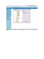
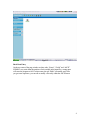
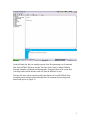
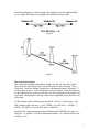
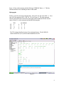
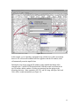
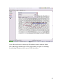
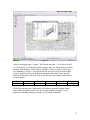
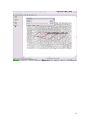
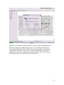
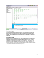
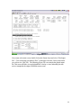
PCSWMM 2002 EXTRAN Block
PAT AVENUE – Storm Drainage Design
A “Hello World” Example Prepared by Dr. Robert Pitt and Jason Kirby,
Department of Civil Engineering, University of Alabama
August 20, 2002
Introduction
SWMM, the EPA’s Storm Water Management Model, is probably the most commonly
used model for evaluating and designing large and complex urban drainage systems. It is
frequently used to investigate: overflows and other problems in combined sewers (CSOs)
/ separate sanitary sewers (SSOs), sewer rehabilitation options, management options to
decrease basement flooding, and the typical designs of new sanitary / storm drainage
systems. Numerous SWMM resources are available through the University of Guelph,
while the latest model versions (along with essential documentation for PCSWMM) can
be downloaded at:
http://www.chi.on.ca/swmm.html
The following example is a simple “Hello World” analysis used to evaluate a small storm
drainage system utilizing the EXTRAN block in PCSWMM2002. Extran (Extended
TRANsport) is a hydraulic flow routing model for open and/or closed conduit systems.
Extrans is utilized whenever it is important to represent severe backwater conditions and
special flow devices such as weirs, orifices, pumps, storage basins, and tide gates. This
simple example will demonstrate how to set up a model for analysis and examine the
resulting output. The provided screen shots will illustrate all of the steps required to
create the input file.
Starting the PCSWMM2002 Program
To start the program, go to the shortcut located on your desktop (see Figure 1), or select
Start/Programs/PCSWMM2002. In most cases, the opening screen will appear. However,
in some installations, you may be asked for a password key.
1
Figure 1
Creating a New Project
PCSWMM generates a folder for each project. Inside the folder, the project models are
created. Create a new folder: File/New/Create New Folder. Select the directory for the
location on the computer (using browse), type in a folder name (Extran Model for
example), then press “Create Folder” (see Figure 2). Each element used in the model is
called an “Object” of the project folder.
In this example, you will create a Sanitary Sewer simulation using the EXTRAN block of
PCSWMM2002. Go to File/New/Create New Object. Under object type, drop down the
menu and select a EXTRAN object type. Type in a name in the upper field (Pat Extran
for example), and select “Create Object”. An object will then be created (a square made
of pipe elbows) with a red flag in the front (see Figure 3). The red flag represents that the
object has errors (incomplete data) or has not been executed by PCSWMM. Double click
on the Extran object and select “Edit Input File.”
2
Figure 2
3
Figure 3
Basic Data Entry
On the top center of the page window are three tabs: “Forms”, “Fields” and “ASCII”.
SWMM is very strict about the position of each variable in the input file; a wrong space
will cause the program to fail. For that reason, the tab “Fields” is normally used. Once
you get some experience, you can edit or modify a file easily within the ASCII format.
4
Figure 4
On the left-hand side, there are multiple sections of the file representing sets of command
lines. Each EXTRAN file has at least the Title Lines, Run Control, Conduits/Channels,
Junctions, Boundary Conditions, and Hydrographs. Along the bottom of the screen there
is the help window which describes each cell, when the field form is used.
Each new file starts with an asterisk symbol in the first line, the word $EXTRAN in the
second line, and an asterisk symbol in the third line. The comment lines also begin with
asterisk and space (see Figure 4).
5
Figure 5
Locate the cursor on the fourth line, below the second asterisk. Press enter to create a new
asterisk and line. Now on the left menu do a double click on the word “Title lines”.
Double click on the line A1. A new menu will prompt: Select one copy and check the box
that includes the comments, then click the “Insert” button. This is the title of the object.
Two lines will appear. The first one is a comment line that indicates that the next line is a
title. In the second line, A1 appears which represents the first line of the title section.
Notice that the description of this line appears in the help menu. A green cell with the
number zero will also appear. Click on the “ASCII” Tab located in the top of this
window. Replace this zero with the Title of your project inside single quotes. Click on the
“Field” tab to return to the field environment. Two title lines are usually used to describe
a project. Locate the cursor on the asterisk located below the line A1. Press enter to insert
a new line. Locate the cursor in the line below the line A1 again. Double click on A2 in
the left menu. This will insert a new title line. Don’t include the comments for this line.
Repeat the same steps used for line A1. After you finish, include an additional asterisk
line (see Figure 5).
6
The following diagrams are basic drawing of the purposed sewer-line and should help
you to visualize the system as we manually enter data into the Extran model.
Figure 6
Figure 7
Run Control Information
Run control data is included in the B block. Double click the “B1 Time Step Control”
option under the “Run Control/ Print Control” title on the left side of the page. Select
“Insert Line”, check the “Include Comment Line with Parameter Names” and enter a “1”
for the number of copies. A title corresponds to each cell location. Notice that when you
use the keyboard arrows to move between the cells, the description of each possible value
is presented. The hyperlink, in the help window (lower right hand corner), describes each
cell in detail.
For this example enter the following data into line B1. NTCYC (# of time steps) = 500,
DELT (length of time step in sec.) = 20.0, TZERO = 0.0, NSTART = 1, INTER = 1,
JNTER = 20, REDO = 0, and IDATZ (date) = 20020409.
Insert a B2 line, with comments, and enter the following data. METRIC (US units) = 0,
NEQUAL = 0, AMEN = 0, ITMAX (Maximum Iterations) = 30, AND SURTOL (Flow
Fraction) = 0.05.
7
Insert a B3 line, with comments, and enter the following data. NHPRT (# of manholes) =
3, NQPRT (# of pipes) = 2, NPLT = 0, LPLT = 0 and NJSW = 2.
Insert a B4 line, with comments, and enter the following data. 300, 301, and 302. This
line lists the manholes.
Insert a B5 line, with comments, and enter the following data. 3000 and 3001. This line
lists the pipes.
(See Figure 8)
Figure 8
Conduits and Channels
The next lines to be added are C1, located under Conduits/Channels. Add 3 copies, with
comments, and leave blank. Data will be created later utilizing the GIS module.
Junctions
The next lines to be added are D1, located under Junctions. Add 2 copies, with
comments, and leave blank. Data will be created later utilizing the GIS module.
Boundary Conditions
Insert 1 copy of line I1 (include comments) located under the Boundary Conditions. Enter
the following data: JFREE (location of outfall) = 302, and NBCF = 1.
8
Insert a J1 line (with comments) with the following: NTIDE (BC Index) = 1. This line
indicates that there is no controlling structure on the outfall.
Hydrographs
Finally, we need to enter the hydrograph data. Insert a K1 line and enter NINC =1. Next
enter a K2 line and enter JSW = 300 301 302 (see Figure 9). The most important
element of the EXTRAN model is flow hydrograph entered within the K3 lines. Insert 4
copies of line K3, ( with comments) and enter the following data.
K3
K3
K3
K3
TEO
0
1
1.5
4
0
5
0
0
QCARD(X)
0
0
7
5
0
0
0
0
The TEO column identifies the time of day (in decimal hours). The QCARD (X)
column list the flow (in cfs) at the locations identified in line K2.
Figure 9
9
SAVE THE FILE WITHOUT RUN (the far left “diskette” icon on the top tool bar).
Don’t close the window.
GIS Runoff Module to Enter Pipe Information
Create a new object from the PCSWMM2002 window. Select GIS object and assign a
name. The object is an earth symbol that will be created in the project window. You may
have to drag the Pat Extran and Pat GIS objects apart by holding down the left mouse
button and moving one, as they may super-imposed on top of each other.
Double click the GIS object. On the left side are the SWMM modules that can interface
with the GIS module: Runoff, Transport and Extrans. Check the little box to activate the
Extrans model and deactivate the Runoff and Transport modules. Click on the word
Extrans to activate the Extrans module (a shadow box will be created around the
EXTRAN module if done correctly) (see Figure 11).
Optional Import of Images into the GIS Module
It is possible to import a site image (such as a topographical map or an aerial photograph)
into the GIS window to make placement of the drainage elements easier. However, this is
not required, and the elements can simple be placed on a blank screen.
Import the image of the site by selecting “connect background layer,” located in the “file”
drop down menu. Browse to locate the desired image (Patwatershed.jpg) on your
computer, select “Open,” and then select “Connect” (see Figure 10). When the program
asks for the reference file, chose “Cancel”. This option is for georeferenced images that
are not needed (and not available for this example). When the image is registered, a text
file locates the image in map coordinates. For this example, there are no such referencing
files. To enlarge or reduce the image in the GIS window, click on the + and – icons in the
top tool bar and then click on the image.
10
Figure 10
In this example, we are importing a topographic map with the Sewer’s Sub-areas already
drawn in. We will locate the manholes and sewer pipelines with the GIS module, which
will automatically create the input file lines.
Entering the sewer layout, using the GIS module, greatly simplifies the linkage of the
elements to the C1 and D1 EXTRANs block lines. With the second icon located in the
top GIS toolbar, add the conduits. Click the pipe junctions from the upslope to the
downslope direction. Nodes (manholes) 300, 301, and 302 along with Pipes 3000, and
3001, will be created automatically (see Figure 11).
11
Figure 11
Use the first icon (the arrow) from the top GIS toolbar to select the elements. Double
click on the first pipe, number 3000. A new popup window (see Figure 12) will display
the positioning of the pipe, and allow you to modify its attributes.
12
Figure 12
Select a circular pipe (type 1), length = 300 ft, depth and width = 1 ft, and invert 1 and 2
= 0.5 ft(see Figure 13). In the Extran block, the pipe slopes are determined by the relative
elevation of the manholes. If the material of the pipe is concrete (which it is here), then
use a Manning’s n of 0.013. The required units, for each cell, may be found in the help
window’s hyperlink. When you are finished entering the first conduit’s data, click the x
button in the top right corner of the entry screen. Enter the other conduits’ information in
the same manner.
Pipe
3000
Type
Circular
Length
300
Invert 1
0.5
Invert 2
0.5
Roughness
0.013
Use the first icon (the arrow) from the top GIS toolbar to select the elements. Double
click on the first manhole, number 300. A new popup window (see Figure 13) will
display the positioning of the pipe, and allow you to modify its attributes.
13
Figure 13
Only the ground elevation and invert elevation need to be modified. Leave the inflow
and initial depth values equal to zero. Enter the following elevations in the appropriate
nodes.
Manhole
Ground Elevation
Invert Elevation
300
500’
490’
301
478.1’
468.1’
302
461.3’
451.3’
These values will give pipe 3000 a 7.3% slope and pipe 3001 a 5.6% slope.
Linkage of GIS file with Extran Block
Link the GIS with the extran file by selecting “Associated Input Files” from the “View”
drop down menu. Chose the “Extran File” option and browse to the edited input file.
Once the file has been located, select “Update,” then select “Close” (see Figure 14).
To update the edited file, select from the “File” dropdown menu and select the “Update
Extran Input File” option. The window will show “Entries for Export” (select “All
Entries on Layer”) and “Scope of Replacement” (select “Replace All Entries”), and then
click on “Update” (See Figure 15).
14
Figure 14
15
Figure 15
Minimize the GIS window and go to the input file. The edit window will prompt that the
file has been changed by another program, click “Yes” to refresh from file. Figure 16
shows that the information in the C1 and D1 lines have been changed to reflect the data
entered in the GIS module. At this time, take a look at the input file to ensure all the
information is present and no data entry errors have been made. Once the file has been
updated and reviewed, you will be ready to run the program.
16
Figure 16
Running the Program
Save and run the program by clicking on the save / run icon on the top tool bar, or by
double clicking on the runoff icon in the main PCSWMM screen and selecting “Run
SWMM”. Once the input file has been successfully run you will be able to examine the
output file.
Reviewing the Output
Return to the main PCSWMM2002 screen. The red flag in front of the Extran Object
(pipe square) will have been removed, meaning that the input file has been executed.
Double click on the Extran object and select “View Output File”. The output file will
detail selected output hydrographs and list the average flow, velocity, max & min flow,
as well as the average percent change within the manholes and pipes. Make sure that the
“Transport Simulation ended normally (See Figure 17).
17
Figure 17
Next, return to the main screen, double click on the Extran object and select “Plot Output
File”. Click on the drop icon labeled “Flow” in the upper left corner. Select which nodes
you wish to view (300-302). The following (Figure 18) is an example the plotted output
file. This screen will allow you to plot depth/flow/ velocity vs. time, and modify the time
series to manipulate the output for different storm events.
18
Figure 18
Viewing the Dynamic HGL
The most interesting feature of the Extran model is viewing the predicted HGL. Double
click on the Extran object and select “View Dynamic HGL”. Select all the junctions
(300-302) and hit “OK”. A profile view of the pipe system will appear. Press the “Play”
button in the lower left hand corner to see how the flow moves thru the pipe. You should
notice that the flow overtops manhole 301 at one hour (red circle), this indicates system
failure. Enlarging the pipes or manipulating the flow volumes can eliminate these
failures.
You can edit (and rerun) the input file to view different flow profiles.
Entering,
K3
K3
K3
K3
0
0
1
10
1.5 0
4
0
0
7
0
0
0
5
0
0
will result in a double failure at manholes 300 and 301.
19
Entering,
K3 0
0
0
0
K3 1
5
7
5
K3 1.5 0
0
0
K3 4
0
0
0
doesn’t result in a failure, however you can see where the flow begins to move up
manhole 301 before receding. The figures below display examples of these failures.
Figure 19
20
Figure 20
A Few SWMM References
James, W., W.C. Huber, R.E. Dickinson, and W.R.C. James. Water Systems Models:
Hydrology, Users Guide to SWMM4 RUNOFF and Supporting Modules. CHI. Guelph.
1999
James, W., W.C. Huber, R.E. Dickinson, L.A. Roesner, J.A. Aldrich, and W.R.C. James.
Water Systems Models: Hydrology, Users Guide to SWMM4 TRANSPORT, EXTRAN and
STORAGE Modules. CHI. Guelph. 1999.
Huber, W.C., Heaney, J.P. and B.A. Cunningham. Storm Water Management Model
(SWMM) Bibliography. EPA/600/3-85/077 (NTIS PB86-136041/AS), U.S. EPA, Athens,
GA, September 1985.
Huber, W.C. and R.E. Dickinson. Storm Water Management Model, Version 4, User’s
Manual. EPA/600/3-88/001a (NTIS PB88-236641/AS), U.S. EPA, Athens, GA, 30605.
1988.
21
Metcalf and Eddy, Inc., University of Florida, and Water Resources Engineers, Inc.
Storm Water Management Model, Vol. I. Final Report, 11024DOC07/71 (NTIS PB203289), U.S. EPA, Washington, DC, 20460. 1971.
Roesner, L.A., Aldrich, J.A. and R.E. Dickinson. Storm Water Management Model,
Version 4, User's Manual: Extran Addendum. EPA/600/3-88/001b (NTIS PB88236658/AS), U.S. EPA, Athens, GA, 30605. 1988.
22