Download basic Pat Ave RUNOFF Storm Drainage example

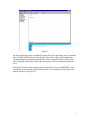
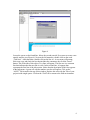
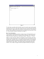
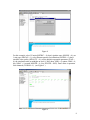
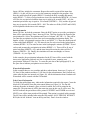
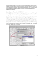
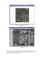
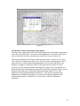
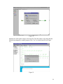
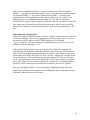
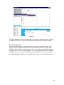
PCSWMM 2002 RUNOFF Block
PAT AVENUE – Storm Drainage Design
A “Hello World” Example Prepared by Robert Pitt and Alex Maestre, Department
of Civil Engineering, University of Alabama
April 10, 2002
Introduction
SWMM, the EPA’s Storm Water Management Model, is probably the most commonly
used model for evaluating and designing large and complex urban drainage systems. It is
frequently used to investigate: overflows and other problems in combined sewers (CSOs)
/ separate sanitary sewers (SSOs), sewer rehabilitation options, management options to
decrease basement flooding, and the typical designs of new sanitary / storm drainage
systems. Numerous SWMM resources are available through the University of Guelph,
while the latest model versions (along with essential documentation for PCSWMM) can
be downloaded at :
http://www.chi.on.ca/swmm.html
The following example is a simple “hello world” analysis used to create a minimal storm
drainage evaluation using the RUNOFF block in PCSWMM2002. The RUNOFF block
contains information on precipitation, land use, and optionally (as in this example),
sewerage data. Plumbing information is more commonly given in the TRANSPORT or
EXTRANS blocks. This simple example will demonstrate how to set up a model for
analysis and examine the resulting output. The provided screen shots will illustrate all of
the steps required to create the input file.
RUNOFF is quite limited in its capabilities, and while the program block can evaluate a
drainage system, it is unable to provide a design. It does, however, show how a SCS Type
II design storm can be imported for use. PCSWMM2002 contains multiple examples
(data sets) which illustrate the various features available within the RUNOFF block
program. Of special interest is example set #4 which shows how to do stormwater sizing
automatically (using a combination of the RUNOFF and TRANSPORT blocks, or an
equivalent, but more powerful combination of the RUNOFF and EXTRANS blocks). In
transport, the sewerage can be re-sized by setting NDESN = 1 in line B3 (The initial pipe
diameters should all be set equal to the minimum pipe dimensions allowed by the
reviewing agency and the output file will calculate the pipe diameters needed to prevent
drainage failure. The resulting pipe dimensions have to be corrected to available
commercial sizes and the model re-run for final analysis).
Another good example to look at is set #5 which shows how to design a sanitary system.
Starting with the average annual flow, then using modifiers for monthly, weekly, daily,
and finally hourly variations, PCSWMM can be used to obtain the peak flows and
detailed data on flow variations. Automatic re-sizing is also available in TRANSPORT
line B3, as noted above. It is also possible to add precipitation and land use information
from the RUNOFF block to consider I/I (inflow and infiltration) in a separate sanitary
1
system in order to model SSOs (sanitary sewer overflows) or runoff in a combined sewer
system to model CSOs (combined sewer overflows). Both of these example sets contain
blank templates that have all necessary command lines already in place, allowing for
easier data entry using the field option.
Starting the PCSWMM2002 Program
To start the program, go to the shortcut located on your desktop, or select
start/programs/PCSWMM2002. In most cases, the opening screen appears. However, in
some installations, you may be asked for a password key.
Figure 1
2
Figure 2
Creating a New Project
PCSWMM generates a folder for each project. Inside the folder, the project models are
created. Create a new folder: File/New/Create New Folder. Select the directory for the
location on the computer (using browse) and then type in a folder (project) name, and
then press “create folder.” Each model or element used in the model is called an “Object”
inside of the project.
Figure 3
3
In this example, you will create a Precipitation-Runoff simulation using the RUNOFF
block of PCSWMM2002. Go to File/New/Create New Object. Under object type, drop
down the menu and select a RUNOFF object type. Type in a name in the upper field (Pat
Runoff for example), and select “Create Object” (see Figure 3). An object will then be
created, it will looks like a watershed with a red flag in the front (see Figure 4). The red
flag represents that the object has errors (incomplete data) or has not been executed by
PCSWMM. Double click on the runoff object and select “Edit Input File.”
Figure 4
Basic Data Entry
On the top center of the page window are three tabs: “Forms”, “Fields” and “ASCII”.
SWMM is very strict about the position of each variable in the input file; a wrong space
will cause the program to fail. For that reason, the tab “Fields” is normally used. Once
you get some experience, you can edit or modify a file easily within the ASCII format.
4
Figure 5
On the left-hand side, there are multiple sections of the file representing sets of command
lines. Each RUNOFF file has at least the Title Lines, Run Control, Precipitation Data,
Conduits/Channels, Subcatchments and Print Control. Along the bottom of the screen
there is the help window that explains the description of each cell when the field form is
used.
Each new file starts with an asterisk symbol in the first line, the word $RUNOFF in the
second line, and an asterisk symbol in the third line. The comment lines also begin with
asterisk and space (see Figure 5).
5
Figure 6
Locate the cursor on the fourth line, below the second asterisk. Press enter to create a new
asterisk and line (see Figure 6). Now on the left menu do a double click on the word
“Title lines”. After that make a double click on the line A1. A new menu will prompt.
Select one copy and check the box that includes the comments, the click the “Insert”
button. This is the title of this object. Two lines will appear. The first one is a comment
line that indicates that the next line is a title. In the second line, A1 appears that
represents the first line of the title section. Notice that the description of this line appears
in the help menu. A green cell with the number zero also will appear. Click on the
“ASCII” Tab located in the top of this window. Replace this zero with the Title of your
project inside single quotes. Click on the “Field” tab to return to the field environment.
6
Figure 7
Two title lines are usually used to describe a project. Locate the cursor on the asterisk
located below the line A1. Press enter to insert a new line. Locate the cursor in the line
below the line A1 again. Double click on the line A2 in the left menu. This will insert a
new title. Don’t include the comments for this line. Repeat the same steps used for line
A1. After you finish, include an asterisk line (see Figure 7).
Run Control Information
The run control is included in the B block. Double click the “B1 Modeled Processes”
option under the “Run Control” title on the left side of the page. Select “Insert Line”,
check the “Include Comment Line with Parameter Names,” and enter a “1” for the
number of copies of the line. Each title corresponds to each cell location. Notice that
when you use the keyboard arrows to move between the cells, the description of each
possible value is presented. There is a hyperlink in the help window (lower right hand
corner) that presents the description of each line in detail. Locate the cursor with the
keyboard arrows in the “Metric” cell of line B1 and press the hyperlink in the help
window. A new window will appear with the description of this line (see Figure 8).
7
Figure 8
For this example, select US units (METRIC = 0), don’t simulate snow (ISNOW = 0), use
1 rain gage (NRGAG = 1), select Horton equation for infiltration (INFILM = 0), don’t
simulate water quality (KWALTY = 0), use the default evaporation parameter (IVAP =
0), the simulation starts at midnight on April 9, 2002 (hour, NHR = 0; minute, NMN = 0;
day, NDAY = 9; month, MONTH = 4; year, IYRSTR = 2002). Don’t allow evaporation
from channels (IVCHAN =1). (see Figure 9 )
Figure 9
8
Insert a B2 line, include the comments. Request the model to print all the input data
(IPRN1 = 0), this will let you to review the parameters assigned in the program. Also,
have the model plot all the graphs (IPRN2 = 0) and all the daily, monthly and annual
totals (IPRN3 = 2). Select zero groundwater errors (Not simulated) (IRPNGW = 0). Insert
a B3 line, the wet period calculation time step is equal to 60 seconds (WET = 60), the
transition period time step is equal to 120 seconds (WETDRY = 120), and the dry period
time step is equal to 900 seconds (DRY = 900. The other two fields (LUNIT and LONG)
will be updated with the times series manager.
Rain Information
Insert a D1 line, include the comments. Enter the ROPT option as zero (the precipitation
data will be entered using E lines). Insert an E1 line. This line describes the format of the
precipitation file. Select “Precipitation and Time in Columns” (KTYPE = 2). This will let
you enter the precipitation in pairs (time and corresponding precipitation depth). The
number of time / precipitation events per line is one (KINC = 1). Have the model print all
of the rainfall data (KPRINT = 0). The interval time for each record in the hydrograph is
constant (KTHIS = 0). The units for time in the hydrograph is minutes (KTIME = 0) and
each record presents the precipitation in inches (KPREP = 1). There will be 49 sets of
paired rain data (NHISTO = 49), and the time interval between the values will be 30
minutes (THISTO = 30). Finally, the simulation will start at midnight, or 0 hours
(TZRAIN = 0). (see Figure 10)
In this example, the precipitation information for the E3 lines will be created with the
times series application, and only one line is required for now, assuming zero
precipitation. Add one E3 line now. To create the pair data of the hydrograph (E3), use
the space bar to indicate precipitation zero at time zero.
Watershed Information
In this example there are two conduits and three subcatchment. Insert two (2) copies of
G1 lines for the conduits and three (3) H1 lines for the subcatchments. Don’t include any
values after the lines are inserted (see Figure 10). All the information about Conduits and
Watersheds will be created with the GIS module.
Print Control Information
To finish the manual data entry, indicate the information required in the report. Create the
blocks M1, M2 and M3 from the print control Menu (see Figure 10). The line M1
indicates the nodes in channels, pipes or inlets for which flow will be printed in the
output file. The print interval will be the same time step (in this case it will be one). The
line M2 indicates the period that will be printed. If STARTP and STOPPR are zero and
NDET is one, all the time periods will be printed. That option is required in this example.
The M3 line will be included after using the GIS module. SAVE THE FILE WITHOUT
RUN (the far left “diskette” icon on the top tool bar). Don’t close the window.
9
Figure 10
GIS Runoff Module to Enter Pipe Information
Create a new object from the PCSWMM window. Select GIS object and assign a name.
The object is an earth symbol that will be created in the project window. You may have
to drag the Pat Runoff and Pat GIS objects apart by holding down the left mouse button
and moving one, as they may super-imposed on top of each other (see Figure 11).
Figure 11
10
Double click the GIS object. On the left side are the SWMM modules that can interface
with the GIS module: Runoff, Transport and Extrans. Check the little box to activate the
runoff model and deactivate the Transport and Extrans modules. Click on the word runoff
to activate the Runoff module (a shadow box will be created around the RUNOFF
module if done correctly).
Optional Import of Images into the GIS Module
It is possible to import a site image (such as a topographical map or an aerial photograph)
into the GIS window to make placement of the drainage elements easier. However, this is
not required, and the elements can simple be placed on a blank screen.
Import the image of the site by selecting “connect background layer,” located in the “file”
drop down menu. Browse to locate the desired image (Patwatershed.jpg) on your
computer, select “Open,” and then select “Connect” (see Figure 12). When the program
asks for the reference file, chose “Cancel”. This option is for georeferenced images that
are not needed (and not available for this example). When the image is registered, a text
file locates the image in map coordinates. For this example, there are no such referencing
files. To enlarge or reduce the image in the GIS window, click on the + and – icons in the
top tool bar and then click on the image.
Figure 12
11
From Mapquest’s Globexployer web site:
Figure 13
From the USGS’s Terraserver website:
Figure 14
In this example, we are importing a topographic map with the inlet subdrainage areas
already drawn in. We will locate the inlets and the drainage with the GIS module, which
will automatically create the input file lines.
12
Entering the drainage system and subcatchment locations using the GIS module greatly
simplifies the linkage of the elements on the G1 and H1 RUNOFF block lines. With the
second icon located in the top GIS toolbar, add the conduits. Click the pipe junctions
from the upslope to the downslope direction. Nodes 100, 101 and 102, along with Pipes
1000 and 1001, will be created automatically.
Figure 15
Select the third icon from the top GIS toolbar to locate the subcatchments. Click on the
nodes 100, 101 and 102 where each subcatchment drains. Subcatchments 1001, 1011 and
1021 will be created
13
Figure 16
Use the first icon (the arrow) from the top GIS toolbar to select the elements. Double
click on the first conduit (number 1000). Select a circular type (2), and enter the
appropriate values: a length of 300 ft. and a slope of 7.3% (see Figure 17). In the
RUNOFF block, the pipe slopes are entered as ft/ft (vertical to horizontal inverted slope),
not as %, so enter 0.073 here. However, in the TRANSPORT block, the pipe slopes are
entered as ft/100ft, or as a %. The required units, for each cell, may be found in the help
window’s hyperlink.
If the material of the pipe is concrete, then a Manning’s n of 0.013 is suitable. The width
(pipe diameter) used here is 1 ft. (make sure you don’t use any size smaller than the
minimum pipe size allowed by the reviewing agency). Again, in the TRANSPORT
module where automatic re-sizing is being used, it is recommended that the minimum
allowed pipe diameter be entered for all pipes, and the program will re-size the pipes
automatically in the output file. In the RUNOFF block, this option is not available, so the
actual pipe sizes must be used.
Enter a zero for “Full Depth”, the program will not run for with any other value (values
greater than zero are used for open channels). When you are finished entering the conduit
data, click the x button in the top right corner of the entry screen. Now enter the
information for the other conduit. Pipe 1001 is 300 ft long, with a minimum diameter of 1
ft., a 5.6% (0.056) slope and is concrete (n = 0.013).
14
Figure 17
GIS Module to Enter Subcatchment Information
The image can be temporarily removed by deselecting the lowest checkbox (image name)
on the left of the GIS screen. To enter the subcatchment data, use the first icon selector
(arrow) and double click the watershed icon on the GIS screen (see Figure 18).
The first subcatchment (1001) has the following characteristics: an area of 1.067 acres,
54% of the area is impervious (add 54, not 54%), an average catchment slope of 8.4%
(entered as ft/ft, vertical to horizontal dimensionless ratio, so enter 0.084 here), and
Manning’s roughness coefficients of 0.04 for the impervious area and 0.41 for the
pervious area. The watershed width is determined by using the ratio of watershed area
divided by hydraulic flow length (the longest flow path in the watershed). In this case, the
hydraulic flow path was 473 ft and the resulting watershed width is 98.3 ft. The
parameters for the Horton infiltration equation are: 1 in/hr for the maximum initial
infiltration rate (infiltration1 parameter), 0.1 in/hr for the minimum infiltration rate
(infiltration2 parameter), and 0.002 sec-1 for the decay coefficient (infiltration3
parameter).
15
Figure 18
The second subcatchment (1011) has the following characteristics: 74.5 ft watershed
width, an area of 1.087 acres, 54% impervious area, 9.3% slope (0.093 ft/ft), Manning’s
coefficients for impervious areas of 0.04 and 0.41 for pervious areas. Horton infiltration
parameters are: maximum initial infiltration rate = 1 in/hr, minimum infiltration rate = 0.1
in/hr, and the decay coefficient = 0.002 sec-1.
The third subcatchment (1021) has the following characteristics: 109 ft watershed width,
an area of 1.431 acres, 54% impervious area, 7.2% slope (0.072 ft/ft), Manning’s
coefficients for impervious areas of 0.04 and 0.41 for pervious areas. Horton infiltration
parameters are: maximum initial infiltration rate = 1 in/hr, minimum infiltration rate = 0.1
in/hr, and the decay coefficient = 0.002 sec-1.
16
Figure 19
Linkage of GIS file with RUNOFF Block
Link the GIS with the runoff file by selecting “Associated Input Files” from the “View”
drop down menu. Chose the “Runoff File” option and browse to the edited input file.
Once the file has been located, select “Update,” then select “Close” (see Figure 19).
To update the edited file, select from the “File” dropdown menu and select the “Update
Runoff Input File” option. The window will show “Entries for Export” (select “All
Entries on Layer”) and “Scope of Replacement” (select “Replace All Entries”), and then
click on “Update” (See Figure 20).
17
Figure 20
Minimize the GIS window and go to the input file. The edit window will prompt that the
file has been changed by another program, click “Yes” to refresh from file (see Figure
21).
Figure 21
18
Now you can complete the M lines. Go to the previously entered M1 line and enter
NPRNT = 3 (to print out information for all 3 nodes). We will obtain a complete printout
by selecting INTERV = 1. Go to the M2 line and select NDET = 1, then the total
simulation period will be printed (leave the other two fields as 0). Go to the M3 line.
Indicate that you want information from the nodes 100, 101 and 102: go into the
RUNOFF block input file editor and go to the M3 line. Add 100, 101, and 102 in the first
three fields; enter 100 in the first field, press the space bar to move to the second field
and enter 101, and space to the third field to enter 102. Be sure to periodically save the
file.
Importing Time Series Rain File
Return to the main PCSWMM window. Under the “Utilities” drop down menu, select the
“Timeseries Manager.” Browse to the appropriate rain file and select “Open.” A plot of
the time series will be shown. In the PCSWMM directory is a file labeled
“Type_II_Storm.tsf.” This file contains the precipitation data for a SCS Type II event
(duration =24 hours and depth = 1 in).
In the editing function window, you can create any Type II storm by automatically
modifying the rain depth total. In the edit drop down menu, select the “Edit Timeseries”
option. Select the multiply option and enter 6.9 to obtain a Type II storm having a total
storm depth of 6.9 inches (see Figure 22). Press “Execute”, making sure you only hit the
execute button once. This will generate the new precipitation file. Now you can export
the new precipitation time series to the Runoff file. Use the option “Export” in the drop
down “File” menu, click on “Selected Time Series,” and choose “To Existing SWMM
Input File.” Browse and select the runoff file to be modified, and click on “Export.”
Now go to the input file editor to review the changes. Importing the time series may
modify some of the previously entered data for compatibility (such as the number of rain
increments, and the start date of the event).
19
Figure 22
The Edit window may ask you to update the file. Accept the changes, and save (without
running the file). Now you have all the required information and can run the program.
Running the Program
Save and run the program by clicking on the save / run icon on the top tool bar, or by
double clicking on the runoff icon in the main PCSWMM screen and selecting “Run
SWMM.” You can then view the time series plots, or view the output file, by selecting
the appropriate icons. The following (Figure 23) is an example the output file selected by
clicking on the icon on the top tray of the main PCSWMM window. You can select the
specific hydrographs to display by selecting the junction boxes to the left of the screen.
20
Figure 23
A Few SWMM References
James, W., W.C. Huber, R.E. Dickinson, and W.R.C. James. Water Systems Models:
Hydrology, Users Guide to SWMM4 RUNOFF and Supporting Modules. CHI. Guelph.
1999
James, W., W.C. Huber, R.E. Dickinson, L.A. Roesner, J.A. Aldrich, and W.R.C. James.
Water Systems Models: Hydrology, Users Guide to SWMM4 TRANSPORT, EXTRAN and
STORAGE Modules. CHI. Guelph. 1999.
Huber, W.C., Heaney, J.P. and B.A. Cunningham. Storm Water Management Model
(SWMM) Bibliography. EPA/600/3-85/077 (NTIS PB86-136041/AS), U.S. EPA, Athens,
GA, September 1985.
Huber, W.C. and R.E. Dickinson. Storm Water Management Model, Version 4, User’s
Manual. EPA/600/3-88/001a (NTIS PB88-236641/AS), U.S. EPA, Athens, GA, 30605.
1988.
Metcalf and Eddy, Inc., University of Florida, and Water Resources Engineers, Inc.
Storm Water Management Model, Vol. I. Final Report, 11024DOC07/71 (NTIS PB203289), U.S. EPA, Washington, DC, 20460. 1971.
Roesner, L.A., Aldrich, J.A. and R.E. Dickinson. Storm Water Management Model,
Version 4, User's Manual: Extran Addendum. EPA/600/3-88/001b (NTIS PB88236658/AS), U.S. EPA, Athens, GA, 30605. 1988.
21