Download Technical Protocols for Processing, Sputtering and RF Measuring of

UNIVERSITÀ DEGLI
STUDI DI PADOVA
Facoltà di Scienze MM.NN.FF.
Facoltà di Ingegneria
ISTITUTO NAZIONALE
DI FISICA NUCLEARE
Laboratori Nazionali di Legnaro
in collaboration with Confindustria Veneto
MASTER thesis in
“Surface Treatments for Industrial Applications”
Technical Protocols for Processing, Sputtering
and RF Measuring of Niobium-Copper Cavities
Supervisor: Prof. V.Palmieri
Student: Dott. Giulia Lanza
Matr. N°: 884861
Academic Year 2007/08
Smile though your heart is aching
Smile even though its breaking
When there are clouds in the sky, you’ll get by
If you smile through your fear and sorrow
Smile and maybe tomorrow
You’ll see the sun come shining through for you
Light up your face with gladness
Hide every trace of sadness
Although a tear may be ever so near
That’s the time you must keep on trying
Smile, what’s the use of crying?
You’ll find that life is still worthwhile
If you just smile
That’s the time you must keep on trying
Smile, what’s the use of crying?
You’ll find that life is still worthwhile
If you just smile.
...
Charlie Chaplin
ii
CONTENTS
iii
Contents
Introduction
vii
Acronym
ix
1 Basics of superconducting radiofrequency cavities
1.1 Accelerating cavities . . . . . . . . . . . . . . . . . . . . . . . . . . . . . . . . . . .
1.2 Fundamental equations for rf test . . . . . . . . . . . . . . . . . . . . . . . . . . . .
2 Surface treatments
2.1 EP apparatus . . . . . . . . . . . . . . . . . .
2.2 EP software . . . . . . . . . . . . . . . . . . .
2.3 EP of copper cavities . . . . . . . . . . . . . .
2.3.1 EP: the operators equipment . . . . .
2.3.2 EP: preparation of the process solution
2.3.3 EP: the process . . . . . . . . . . . . .
2.3.4 EP: end of the process . . . . . . . . .
2.4 CP of copper cavities . . . . . . . . . . . . . .
2.4.1 SUBU and passivation:the procedure .
2.5 Ultrasonic cleaning . . . . . . . . . . . . . . .
3 High Pressure Water Rinsing
3.1 The HPWR system . . . . . . .
3.2 HPWR Protocol . . . . . . . .
3.2.1 Preliminary Operations
3.2.2 Cavity mounting . . . .
3.2.3 Computer program . . .
3.2.4 Start the process . . . .
3.2.5 End the process . . . . .
.
.
.
.
.
.
.
.
.
.
.
.
.
.
.
.
.
.
.
.
.
.
.
.
.
.
.
.
.
.
.
.
.
.
.
.
.
.
.
.
.
.
.
.
.
.
.
.
.
.
.
.
.
.
.
.
.
.
.
.
.
.
.
.
.
.
.
.
.
.
.
.
.
.
.
.
.
.
.
.
.
.
.
.
.
.
.
.
.
.
.
.
.
.
.
.
.
.
.
.
.
.
.
.
.
.
.
.
.
.
.
.
.
.
.
.
.
.
.
.
.
.
.
.
.
.
.
.
.
.
.
.
.
.
.
.
.
.
.
.
.
.
.
.
.
.
.
.
.
.
.
.
.
.
.
.
.
.
.
.
.
.
.
.
.
.
.
.
.
.
.
.
.
.
.
.
.
.
.
.
.
.
.
.
.
.
.
.
.
.
.
.
4 Sputtering of Niobium Thin Film onto a Copper Cavity
4.1 The vacuum system . . . . . . . . . . . . . . . . . . . . . .
4.2 The cathode . . . . . . . . . . . . . . . . . . . . . . . . . . .
4.2.1 The Cathode Assembly . . . . . . . . . . . . . . . . .
4.2.2 The bias grid components . . . . . . . . . . . . . . .
4.2.3 The bias grid assembly . . . . . . . . . . . . . . . . .
4.2.4 The Cathode insertion . . . . . . . . . . . . . . . . .
4.2.5 The cavity placement on the system . . . . . . . . .
4.3 The Pump down . . . . . . . . . . . . . . . . . . . . . . . .
.
.
.
.
.
.
.
.
.
.
.
.
.
.
.
.
.
.
.
.
.
.
.
.
.
.
.
.
.
.
.
.
.
.
.
.
.
.
.
.
.
.
.
.
.
.
.
.
.
.
.
.
.
.
.
.
.
.
.
.
.
.
.
.
.
.
.
.
.
.
.
.
.
.
.
.
.
.
.
.
.
.
.
.
.
.
.
.
.
.
.
.
.
.
.
.
.
.
.
.
.
.
.
.
.
.
.
.
.
.
.
.
.
.
.
.
.
.
.
.
.
.
.
.
.
.
.
.
.
.
.
.
.
.
.
.
.
.
.
.
.
.
.
.
.
.
.
.
.
.
.
.
.
.
.
.
.
.
.
.
.
.
.
.
.
.
.
.
.
.
.
.
.
.
.
.
.
.
.
.
.
.
.
.
.
.
.
.
.
.
.
.
.
.
.
.
.
.
.
.
.
.
.
.
.
.
.
.
.
.
.
.
.
.
.
.
.
.
.
.
.
.
.
.
.
.
.
.
.
.
.
.
.
.
.
.
.
.
.
.
.
.
.
.
.
.
.
.
.
.
.
.
.
.
.
.
.
.
.
.
.
.
.
.
.
.
.
.
.
.
.
.
.
.
.
.
.
.
.
.
.
.
.
.
.
.
.
.
.
.
.
.
.
.
.
.
.
.
.
.
1
1
2
.
.
.
.
.
.
.
.
.
.
7
8
10
11
11
11
12
13
13
13
15
.
.
.
.
.
.
.
17
17
19
19
20
20
21
22
.
.
.
.
.
.
.
.
23
23
26
27
28
31
33
34
34
iv
CONTENTS
4.4
4.5
4.6
4.7
4.3.1 The Pump down procedure . . . . . . . . . .
The baking system . . . . . . . . . . . . . . . . . .
4.4.1 The baking procedure . . . . . . . . . . . . .
The magnet assembly and the cooling system . . .
4.5.1 Set the cooling system . . . . . . . . . . . .
Sputtering . . . . . . . . . . . . . . . . . . . . . . .
4.6.1 Sputtering Procedure . . . . . . . . . . . . .
Tips to remember for a good sputtering procedure. .
4.7.1 Process Shut Down and System Opening . .
5 Cryogenic apparatus and cavity stand
5.1 The cryogenic laboratory . . . . . . . . . . . . .
5.2 Cavity preparation and mounting on the stand
5.2.1 Coupler and pickup flange . . . . . . . .
5.2.2 Mount the cavity on the cryogenic insert
5.2.3 Venting of the stand pumping line . . .
5.2.4 Cavity pump down . . . . . . . . . . . .
5.2.5 Cavity baking . . . . . . . . . . . . . . .
5.3 Set the thermometers and the resistances . . .
5.4 Stand insertion . . . . . . . . . . . . . . . . . .
5.5 Cryostat and auxiliary system preparation . . .
5.6 Shields pump down and cryostat purging . . . .
5.7 Cryostat cool down . . . . . . . . . . . . . . . .
5.7.1 Liquid nitrogen cool down . . . . . . . .
5.7.2 Liquid helium cool down . . . . . . . . .
5.7.3 Superfluid helium cool down . . . . . . .
5.8 Cryostat warming up . . . . . . . . . . . . . . .
.
.
.
.
.
.
.
.
.
.
.
.
.
.
.
.
.
.
.
.
.
.
.
.
.
.
.
.
.
.
.
.
.
.
.
.
.
.
.
.
.
.
.
.
.
.
.
.
.
.
.
.
.
.
.
.
.
.
.
.
.
.
.
.
.
.
.
.
.
.
.
.
.
.
.
.
.
.
.
.
.
.
.
.
.
.
.
.
.
.
.
.
.
.
.
.
.
.
.
.
.
.
.
.
.
.
.
.
.
.
.
.
.
.
.
.
.
.
.
.
.
.
.
.
.
.
.
.
.
.
.
.
.
.
.
.
.
.
.
.
.
.
.
.
.
.
.
.
.
.
.
.
.
.
.
.
.
.
.
.
.
.
.
.
.
.
.
.
.
.
.
.
.
.
.
.
.
.
.
.
.
.
.
.
.
.
.
.
.
.
.
.
.
.
34
35
37
37
38
40
40
43
43
.
.
.
.
.
.
.
.
.
.
.
.
.
.
.
.
.
.
.
.
.
.
.
.
.
.
.
.
.
.
.
.
.
.
.
.
.
.
.
.
.
.
.
.
.
.
.
.
.
.
.
.
.
.
.
.
.
.
.
.
.
.
.
.
.
.
.
.
.
.
.
.
.
.
.
.
.
.
.
.
.
.
.
.
.
.
.
.
.
.
.
.
.
.
.
.
.
.
.
.
.
.
.
.
.
.
.
.
.
.
.
.
.
.
.
.
.
.
.
.
.
.
.
.
.
.
.
.
.
.
.
.
.
.
.
.
.
.
.
.
.
.
.
.
.
.
.
.
.
.
.
.
.
.
.
.
.
.
.
.
.
.
.
.
.
.
.
.
.
.
.
.
.
.
.
.
.
.
.
.
.
.
.
.
.
.
.
.
.
.
.
.
.
.
.
.
.
.
.
.
.
.
.
.
.
.
.
.
.
.
.
.
.
.
.
.
.
.
.
.
.
.
.
.
.
.
.
.
.
.
.
.
.
.
.
.
.
.
.
.
.
.
.
.
.
.
.
.
.
.
.
.
.
.
.
.
.
.
.
.
.
.
.
.
.
.
.
.
.
.
.
.
.
.
.
.
.
.
.
.
.
.
.
.
.
.
.
.
45
45
52
52
52
53
53
55
55
55
57
57
57
57
58
59
60
.
.
.
.
.
61
61
61
63
63
65
.
.
.
.
.
.
.
.
.
.
.
67
67
69
73
73
73
75
75
75
76
76
77
6 Auxiliary systems for data acquisition, remote control and
6.1 System monitoring and data sharing . . . . . . . . . . . . . .
6.1.1 Hardware and software . . . . . . . . . . . . . . . . . .
6.1.2 Computers set up . . . . . . . . . . . . . . . . . . . . .
6.2 Radiation Safety System . . . . . . . . . . . . . . . . . . . . .
6.2.1 Laboratories evacuation . . . . . . . . . . . . . . . . .
7 Radiofrequency test system
7.1 RF system . . . . . . . . . . . . . . .
7.2 Software . . . . . . . . . . . . . . . .
7.3 Cable Calibration . . . . . . . . . . .
7.3.1 Initial operations . . . . . . .
7.3.2 Forward power calibration . .
7.3.3 Reflected power calibration .
7.3.4 Transmitted power calibration
7.3.5 Internal power calibration . .
7.4 Cavity measurements procedure . . .
7.4.1 Minimum Reflected Power . .
7.4.2 Decay time and Q vs E curve
.
.
.
.
.
.
.
.
.
.
.
.
.
.
.
.
.
.
.
.
.
.
.
.
.
.
.
.
.
.
.
.
.
.
.
.
.
.
.
.
.
.
.
.
.
.
.
.
.
.
.
.
.
.
.
.
.
.
.
.
.
.
.
.
.
.
.
.
.
.
.
.
.
.
.
.
.
.
.
.
.
.
.
.
.
.
.
.
.
.
.
.
.
.
.
.
.
.
.
.
.
.
.
.
.
.
.
.
.
.
.
.
.
.
.
.
.
.
.
.
.
.
.
.
.
.
.
.
.
.
.
.
.
.
.
.
.
.
.
.
.
.
.
.
.
.
.
.
.
.
.
.
.
.
safety
. . . . .
. . . . .
. . . . .
. . . . .
. . . . .
.
.
.
.
.
.
.
.
.
.
.
.
.
.
.
.
.
.
.
.
.
.
.
.
.
.
.
.
.
.
.
.
.
.
.
.
.
.
.
.
.
.
.
.
.
.
.
.
.
.
.
.
.
.
.
.
.
.
.
.
.
.
.
.
.
.
.
.
.
.
.
.
.
.
.
.
.
.
.
.
.
.
.
.
.
.
.
.
.
.
.
.
.
.
.
.
.
.
.
.
.
.
.
.
.
.
.
.
.
.
.
.
.
.
.
.
.
.
.
.
.
.
.
.
.
.
.
.
.
.
.
.
.
.
.
.
.
.
.
.
.
.
.
.
.
.
.
.
.
.
.
CONTENTS
8 Niobium on Copper cavity: thermal oxidation
8.1 Introduction . . . . . . . . . . . . . . . . . . . .
8.2 Cavity history . . . . . . . . . . . . . . . . . . .
8.3 Rf cavity tests . . . . . . . . . . . . . . . . . . .
8.3.1 27-11-08: 4.2K measure . . . . . . . . .
8.3.2 28-11-08: 1.8K measure . . . . . . . . .
8.3.3 11-12-08: 4.2K measure . . . . . . . . .
8.3.4 18-12-08: 4.2K measure . . . . . . . . .
8.4 Conclusion . . . . . . . . . . . . . . . . . . . .
8.5 Results . . . . . . . . . . . . . . . . . . . . . . .
v
.
.
.
.
.
.
.
.
.
.
.
.
.
.
.
.
.
.
.
.
.
.
.
.
.
.
.
.
.
.
.
.
.
.
.
.
.
.
.
.
.
.
.
.
.
.
.
.
.
.
.
.
.
.
.
.
.
.
.
.
.
.
.
.
.
.
.
.
.
.
.
.
.
.
.
.
.
.
.
.
.
.
.
.
.
.
.
.
.
.
.
.
.
.
.
.
.
.
.
.
.
.
.
.
.
.
.
.
.
.
.
.
.
.
.
.
.
.
.
.
.
.
.
.
.
.
.
.
.
.
.
.
.
.
.
.
.
.
.
.
.
.
.
.
.
.
.
.
.
.
.
.
.
.
.
.
.
.
.
.
.
.
.
.
.
.
.
.
.
.
.
.
.
.
.
.
.
.
.
.
79
79
79
81
82
82
82
82
83
83
Conclusions
87
BIBLIOGRAPHY
89
Acknowledgments
91
vi
CONTENTS
vii
Introduction
Dr. Peter Pronovost, a critical-care researcher at Johns Hopkins University, may have
saved more lives than any laboratory scientist in the past decade by relying on a wonderfully simple tool: a checklist. His article, published in The New Yorker, points out the
critical importance of checklists in achieving reliability in highly complex task environments: "..The checklists provided two main benefits. First they help with memory recall...
A second effect is to make explicit the minimum, expected steps in complex processes...".
Checklists are applied routinely in hospital or by pilot for flying an airplane. They are
compulsory every time the process requires several subsequent actions.
The same expedient should be applied to rf cavity treatments. In fact to prepare a
cavity, from the mechanical workshop to the rf test station, several hundred of steps are
performed. In addition several people are involved in the procedures and they have to
be well trained and coordinated. The main aim of this work is providing the sequence
of operations for all the steps a niobium on copper cavity undergoes from the chemical
treatment to the RF measure.
In Legnaro three laboratories are reserved for cavity treatments and analysis:the chemical lab, the sputtering lab and the cryogenic lab.
The chemical lab has the facilities for the surface treatment of single cell cavities as
well as TESLA 3-cell structures. It is possible to treat two cavities (one of copper and one
of niobium) at the same time. In fact, under the extractor fan, there are two completed
circuits, one dedicated to the electropolishing and the chemical polishing of niobium cavities and the other one for copper cavities [1].
There are four ultrasonic bath for cleaning cavities. The chemistry lab provides also a
system for High Pressure Water Rinsing. The HPWR is a system for cleaning cavities at
high pressure with deionized water and it grants the acid and particles removal form the
cavity wall.
The laboratory has one vacuum system for cavity coating. It is structured for 1,5 GHz
and 1,3 GHz tesla type cavity coating and the usual time for one deposition is five days.
The cavity and the cylindrical cathode are assembled and disassembled in a class 1000
clean room to prevent any particle contamination. The vacuum system is located in a
class 10000 clean room.
At the superconductivity lab in Legnaro it’s possible to measure a 1,5 GHz mono-cell
viii
Introduction
cavity in four days: High Pressure Water Rinsing, pump down, cooling, measure at 4,2K
and measure at 1,8K. During the rf test, the cavity has to be cooled at cryogenic temperatures in order to reach the superconducting state. In the rf testing facility there are four
apertures which can host a cryostat. Three of them are used to test QWRs and single
cell TESLA type cavity. This kind of cryostat can hold 100 liters of helium. The last
one is for the multi-cells TESLA type cavity with a volume of 400 liters of helium. This
cryostat has been designed for operating at 4.2K and 1.8K with a maximum power of 70
W. In order to reduce the cooling cost, a preliminary cooling is achieved by using the liquid
nitrogen of the second chamber. Once the temperature reaches 80Kthe transfer of liquid
He at 4.2K into the main vessel is started.Then the temperature of liquid helium can be
lowered decreasing the chamber pressure. The cavity is tested at 4.2K and then at 1.8K,
it is mounted on a vertical stand and it is connected to a pumping line. Remote systems
monitor its temperature, its pressure and the transmission of the radiofrequency.
All the procedures for cavity preparation need qualified and expert operators that
know every sequence of operations. This report is the starting point to train new peoples
and the reference point for the staff working on NbCu cavities.
ix
Acronym
The following is a list of the acronyms used in this thesis:
BMS = Biased Magnetron Sputtering
EP = Electro Polishing
HPWR = High Pressure Water Rinsing
MS = Magnetron Sputtering
PVD = Physical Vapour Deposition
RTD = Resistance Temperature Detectors
RF = Radio Frequency
SRF = Superconducting Radio Frequency
UHV = Ultra High Vacuum
x
Acronym
1
Chapter 1
Basics of superconducting
radiofrequency cavities
1.1
Accelerating cavities
Accelerating cavities are used to increase the energy of a charged particle beam. Obviously, the energy gain per unit length is therefore an important parameter of such devices.
This is conveniently derived from the accelerating voltage to which a particle with charge
e is subjected while traversing the cavity:
¯
¯
¯1
¯
V acc = ¯¯ × energy gain during transit¯¯
e
(1.1)
For particles travelling with the velocity of light c on the symmetry axis in z -direction
(ρ = 0) and an accelerating mode with eigenfrequency ω this gives:
¯Z
¯
V acc = ¯¯
0
d
Ez (z)e
iωz
c
¯
¯
dz ¯¯
(1.2)
The accelerating field is
Vacc
(1.3)
d
Two other key parameters to characterize the superconducting accelerating structures
are Epk and Hpk , which denote the highest electric and magnetic field on the surface
of the resonant structure. In an ideal situation, one can keep feeding the power to the
resonant cavity until the peak magnetic field reaches the critical rf magnetic field Hrf
c , a
little higher than the thermodynamic critical magnetic field for niobium (a meta-stable
superconducting state under superheated critical magnetic field) [2]. For a typical teslatype cavity, the theoretical maximum accelerating gradient is about 55 MV/m [3]. At the
moment the standard Eacc, achievable in the industrial production, is about 25-30 MV/m
for 9-cell working tesla-type accelerating cavities based on bulk niobium material.
In order to sustain the radiofrequency fields in the cavity, an alternating current is
flowing in the cavity walls. This current dissipates power in the wall as it experiences a
Eacc =
2
Basics of superconducting radiofrequency cavities
surface resistance. One can look at the power which is dissipated in the cavity, Pd , to
define the global surface resistance Rsurf :
Pd =
1
2
I
1
2
Rsurf Hsurf
dA = Rsurf
2
A
I
A
2
Hsurf
dA
(1.4)
Here Hsurf denotes the magnetic field amplitude. Usually, one measures the quality
factor Q0 :
ωU
Pdiss
Q0 =
(1.5)
where
1
U = µ0
2
I
H 2 dV
(1.6)
V
is the energy stored in the electromagnetic field in the cavity. Rsurf is an integral
surface resistance for the cavity. The surface resistance and the quality factor are related
via the geometrical constant G which depends only on the geometry of a cavity and field
distribution of the excited mode, but not on the resistivity of the material:
H
H 2 dV
2
A H dA
ωµ0
G= H
V
(1.7)
This gives:
H
ωµ0 V H 2 dV
G
H
Q0 =
=
2
Rsurf
Rsurf A H dA
(1.8)
The quality factor can also be defined as
Q0 =
f
∆f
(1.9)
where f is the resonance frequency and ∆f the full width at half height of the resonance
curve in an unloaded cavity. For the typical elliptical shape of superconducting cavities
G = 270Ω. For a mono-cell TESLA niobium cavity the quality factor is typically Q0 =
1.2×1010 at T = 2 K corresponding to a surface resistance of Rsurf = 10nΩ.
One can see that the efficiency with which a particle beam can be accelerated in a
radiofrequency cavity depends on the surface resistance. The smaller the resistance i.e.
the lower the power dissipated in the cavity walls, the higher the radiofrequency power
available for the particle beam. This is the fundamental advantage of superconducting
cavities as their surface resistance is much lower and outweighs the power needed to cool
the cavities to liquid helium temperatures.
1.2
Fundamental equations for rf test
During the rf tests on cold cavities the basic rf properties such as maximum accelerating gradient, field emission onset, and quality factor Q0 , as a function of gradient are
1.2 Fundamental equations for rf test
3
determined. These tests are done inside the cryostat where the cavity is held vertically.
Ideally, these tests are done at or near critical coupling. In addition to improving the systematic errors, setting the fundamental power coupler at or near critical coupling reduces
the rf power requirement to a value close to that required for cavity wall losses.
The critical variable for calculating the rf parameters of a superconducting cavity is
the shunt impedance, which relates the stored energy to the effective accelerating gradient.
It, along with cavity geometry, is the parameter necessary for calculating peak electric
field, and peak magnetic field for any given mode. In our case it is determined using the
electromagnetic simulation tool called Superfish and all important parameters determined
for 1.5 and 1.3 GHz cavities are collected in tables 1.1 and 1.2 .
Symbol
Variable name
Units
r/q
Geometric shunt impedance
Ω/m
G
Geometry factor
Ω
E
Electric field
V/m
L
Electrical lenght
m
ω0
cavity frequency
s−1
U
Stored energy name
J
Rs
Surface resistance
Ω
Tc
Critical temperature
K
Pemit
Emitted power
W
R
Shunt impedance
Ω
T
Operational temperature
K
Rres
Residual surface resistance
Ω
Q0
Intrinsic quality factor
Qcpl
Fundamental Power coupler coupling factor
Qpk
Field probe coupling factor
RC
Coupling impedance
Ω/m
Pdiss
Dissipated power
W
τ
Decay time
s
r
Shunt impedance per unit length
Ω/m
Table 1.1: Common variables when discussing rf cavities [4].
When a cavity mode oscillates with a resonant frequency ω0 , a stored energy U and rf
losses on the cavity walls, Pd , the quality factor can be defined as:
Q0 =
ω0 U
Pd
(1.10)
Q0 is 2π times the ratio of the stored energy and the energy consumed in one period.
In the frequency domain the Q0 can also be expressed as
4
Basics of superconducting radiofrequency cavities
Q0 =
ω0
∆ω0
(1.11)
where ∆ω0 is the 3-dB band width. Unfortunately, the direct measurement of the 3-dB
band width of a superconducting cavity is practically impossible, because it can attain
very small values as compared to the center frequency: some Hz or fractions of Hz out
of thousands of Megahertz. This is much less than the resolution of any commercially
available network or spectrum analyzer. For this reason, a time domain method must be
used.
The cavity receives the rf power via an input cable and an input antenna (coupler)
from a power amplifier driven by a signal generator which is locked, as explained in the
following chapters, exactly onto the resonant frequency of the cavity mode.
The transmitted power is extracted from the cavity by the output antenna (pickup
probe).
All antennas are connected to calibrated power meters and it is possible to calculate
the total power lost PL with the following power balance:
PL = Pd + Pcpl + Ppk
(1.12)
where Pd is the power dissipated in the cavity walls, Pcpl is the power leaking back out
the fundamental power coupler and Ppk is the power transmitted out via pickup antenna.
This equation is valid for a cavity with no driving term that has a stored energy U.
In this condition the so called "Q loaded" is introduced to take into account the resonant
circuit behaviour when it is coupled with an external line:
QL =
ω0 U
PL
(1.13)
The quality factor, for each dissipated power, could be written as:
Q0 =
ω0 U
Pd
Qcpl =
ω0 U
Pcpl
Qpk =
ω0 U
Ppk
(1.14)
Those Q values are proportional to the number of cycles the system needs to dissipate
all the energy on the considered transmission line. It’s important to control if the dissipated
power in the couplers is higher or lower that the power dissipated on the cavity walls.
It follows that:
1
1
1
1
+
+
=
QL
Q0 Qcpl Qpk
(1.15)
Each transmission line has its own external coupling factor β defined by:
βx =
Q0
Px
=
Qx
Pd
(x = cpl, pk)
(1.16)
As explained in chapter ?? the transmission antenna should be sized in order to avoid
perturbation of the cavity operation, this condition is reached when βpk ¿ 1; in this way
1.2 Fundamental equations for rf test
5
the antenna pickups the bare minimum energy requested for the measurement. Moreover
its position respect to the coupler antenna is far enough to avoid the signal transmission
without resonance inside the cavity (no cross-talking). On the other side, to be able to
transfer all the input power to the cavity, the coupler should satisfy the condition βcpl = 1
(critical coupling). That conditions assure a perfect match of the system and the cavity
electrical impedances (coupling). In fact when βcpl = 1 the input power equals the power
dissipated in the cavity plus the small amount of power that goes out of the pickup port:
Pd = Pi − Pref − Ppk
(1.17)
where Pi is the incident power, Pref is the reflected power and one assumes that
Ppk ¿Pd .
Impedance matching is essential otherwise a mismatch causes power to be reflected back
to the source from the boundary between the high impedance and the low impedance. The
reflection creates a standing wave, which leads to further power waste. As described in the
following sections, the impedance matching device is the antenna tuner. In cases where
β is not equal to 1, such as systems with a fixed input antenna or cavities when used to
accelerate beam, the termination of the stored energy becomes more complex. Detail on
the calculation necessary for such cases are given in reference [4]. Fortunately, our system
allows us to achieve critical coupling prior to doing a decay measurement. This simplifies
the math and allows us to make several assumption which are described below.
When switching off the power supply, the cavity enters into a state of free decay, loosing
energy due to dissipation on the cavity walls and the power flowing through the input and
the output antennas. During a free decay, the power lost corresponds to the variation with
time of the stored energy, thus:
dU
ω0 U
= −PL = −
= −Pd − Ppk − Pcpl
(1.18)
dt
QL
the solution (assuming that QL is independent of U) is an exponential decay, with
QL
(1.19)
ω0
The decay time constant τ is experimentally measured and it is used to calculate a
value for the loaded-Q, QL . Then QL , Pi , Pref , Ppk are used to calculate Q0 . In fact when
the cavity is critically coupled:
t
U = U (0) · e− τ
τ=
Q0 = (1 + βcpl + βpk )QL = 2QL = 2ω0 τ
Qpk =
2ω0 τ (Pi − Pref − Ppk )
Ppk
(1.20)
(1.21)
In summary, measuring Pi , Pref , Ppk and τ are sufficient to derive QL and Qpk . The
next step is increasing the incident power Pi in order to raise the stored energy value U.
Qpk is a constant that is strictly dependent on the probe/cavity geometry. Thus, using
Qpk the Q0 and E values, can be calculated from the measured values of Pi , Pref , Ppk .
6
Basics of superconducting radiofrequency cavities
Q0 =
Qpk Ppk
Pi − Pref − Ppk
(1.22)
The gradient may then be calculated as:
r
E=
Qpk Ppk
r/Q
L2
Parameter
(1.23)
Tesla-type cavity
1.5 GHz
1.3 GHz
2πf
frequency (Hz)
9.425·109
8.168·109
r/q
Geometric shunt impedance (Ω/m)
82.7
82.7
L
Electrical length (m)
0.1
0.1154
G
Geometry factor (Ω)
287
287
Table 1.2: Important parameters when calculating the cavity excitation curve. In this
work both mono-cell 1.5 GHz and 3-cell 1.3 GHz were tested.
7
Chapter 2
Surface treatments
Copper cavities need a peculiar attention to surface treatment because it has been
proved that a reduction in roughness allows for a consistent reduction in film defect density.
In many cases niobium film seems to replicate the copper substrate morphology as the result
of an heteroepitaxial growth mechanism, which favors the growth of some niobium planes
parallel to particular copper planes for which there is a good lattice match[5].
Generally the copper cavities undergo the following sequence of surface treatments (if not
else specified) and processes:
•
•
•
•
•
•
Stripping from the previous coating 1
1 hour electropolishing (at CERN even 5 hours)
High Pressure Water Rinsing (HPWR) 30 minutes at 100 bar
10 minutes chemical etching SUBU (see section 2.4)
10 minutes passivation
High Pressure Water Rinsing (HPWR) 1 hour at 100 bar
In some cases washing in ultrasonic bath were tried, mainly to remove the chemistry residuals.
Electropolishing is an electrochemical process by which surface material is removed by
anodic dissolution. Sometimes referred to as "reverse plating", electropolishing actually
removes surface material, beginning with the high points within the microscopic surface
texture. By removing these points, the electropolishing process will improve the surface
finish, leaving a smoother and more reflective surface.
Electropolishing is accomplished by creating an electrochemical cell in which the material to be polished is the anode. A cathode is formed to mirror the geometry of the
work-surface and the two are submerged in a heated electrolyte bath. When a DC current
is applied, the electrical charge forces metal ions to be dissolved from the work-surface. The
key to the electropolishing process is the difference in current density across the surface.
Within the microscopic surface profile, the current density is greater at the high points and
lesser at the low points. The rate of the electropolishing reaction is directly proportional
1
A niobium chemical etching based on a mixture of Strip Aidr, deionized water and fluoridric acid
8
Surface treatments
to the current density. The increased current density at the raised points forces the metal
to dissolve faster at these points and thus tends to level the surface material. After the
electropolishing treatment, the work-piece is passed through a series of steps to neutralize,
rinse and clean the surfaces.
Electropolishing delivers a smoother, more reflective surface that reduces product adhesion and improves surface cleanability. Perhaps more importantly, electropolishing preferentially dissolves free iron, inclusions, and embedded particles from the surface of the
work-piece. This process improves the near surface chemistry of the material, and promotes the formation of an improved corrosion resistant surface layer.
Chemical polishing (CP) is easier and cheaper then electropolishing, so it is widely
used in many laboratories, but it doesn’t grant good performances at high gradients. The
drawback of BCP as commonly applied is that it etches rather than polishes the surface.
After heavy etching, BCP tends to etch preferentially at grain boundaries, leaving some
crevices, which are difficult to rinse correctly and which enhance the surface roughness.
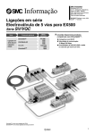
2.1
EP apparatus
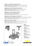
The facility allows for the treatment of single cell cavities as well as TESLA 3-cell structures, and it is also possible to treat two cavities (one of copper and one of niobium) at
the same time (figure 2.2). In fact, under the fume hood, there are two completed circuits,
one dedicated to the electropolishing and the chemical polishing of niobium cavities and
the other one for copper cavities[1].
Cavities are polished in horizontal orientation and are filled with acid at a level of 65%.
All rotating flanges and the fixed structure connected to the cavity are made of PVDF.
The pump chosen is made of PFA and it is an air powered, self priming, diaphragm pumps
with a maximum capacity of 50 l/min at 6 bar. After the pump the acid flow through a
filter (0,2 µm) The tubes, fittings and valves are industrial standard for pure fluid handling
and made of PFA. To force the acid flow, the system is under pressure by a nitrogen flux
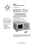
visible in figure 2.1.
It has been observed that it is advantageous to inject the acid downwards in the individual cells, indeed acid flows inside the cathode and get into the cavity passing through its
holes, positioned in correspondence of each cell. This helps also to obtain a better mixing
of "fresh" and "older" acid in the cavity. The acid is then drained on both sides of the
cavity into 1 inch pipes.
While the cathode is kept still, the outer part of the flanges rotates and so does the
cavity. An electrical stepping motor controlled by a computer program provides the rotation. The operator can select the speed, the duration and the direction of the motion. In
all EP processes, the cavity rotates at about 1rpm.
At the end of the process, the power supply and the membrane pump is stopped. The
acid is removed from the cavity volume, by putting the cavity upright. The gravity and
the nitrogen gas overpressure make the acids flow to the acid tank. When the cavity is
2.1 EP apparatus
Figure 2.1: Scheme of the horizontal EP apparatus for copper and niobium cavities
9
10
Surface treatments
empty, the cathode is removed from the upper flange and a water inlet is mounted instead
of it. Thus, the cavity is rinsed until the pH of exiting water is neutral. Furthermore, the
pump and the filter are emptied, and both are connected to the water line for rinsing.
Due to the potential chemical hazard the whole EP system is mounted inside a fume
hood, which also holds inside the exhaust acid tank and the nitric acid solution tank. In
this way any acid droplets that may come out from the EP system is kept inside the hood.
The acid vapor is sucked up through a couple of apertures, by using a 3000 lt/h ventilator.
However, the operator must wear chemical resistant overalls along with a pair of PVDF
gloves and a gas mask.
Figure 2.2: The double horizontal EP apparatus for copper and niobium cavities
2.2
EP software
At LNL two softwares for controlling the electropolishing process have been developed.
The first one is a Visual Basic software. In that case the power supply for monocell
cavities is the HP 6032 (0-60V, 0-50A, 1000W)[6].
2.3 EP of copper cavities
11
The second software is the Automatized Program and it’s written in Labviewr 7.1 RT
instead ??. It can work in connection with the PC or stand alone into the physical memory of NI Field Pointr. When the program works in connection with the computer, all
the parameters can be changed during the process and the display refreshes the polarization curve [7]. The controlled power supply is Alintel mod. HCED125/80 (0-80V, 0-125A).
2.3
EP of copper cavities
The cathode is OFHC copper with a purity of 99.9%, an outer diameter of 25mm and a
wall thickness of 1mm. The standard electro-polishing solution is a Phosphoric acid (85%)
and Butanol (99%) mixture, in the ratio 3:2. The acid storage tank is made of PVDF and
it doesn’t need a water cooling circuit.
2.3.1
•
•
•
•
•
•
•
•
•
Inform the Chemical Lab person in charge for the electropolishing.
Breathing mask with a filter
Protective eyewear
Anti acid suit
Long VITON gloves
Gumboots
Check the eye wash safety station
Cream for the acid neutralization
Solution of boric acid for the gloves rinsing
2.3.2
•
•
•
•
•
•
•
•
•
•
•
EP: the operators equipment
EP: preparation of the process solution
Switch on the fume hood.
Empty the entire plants from water.
Disconnect all pipes to empty them. Use the nitrogen gas for insufflation.
Empty the filter with the proper valve.
Let the pump running freely to empty it.
For a monocell the operator should prepare 15 liters of solution.
Pump 9 liters of Phosphoric acid (85%) in the tank.
Start the stirrer.
Add 6 liters of Butanol (99%).
Stir the solution for 30 minutes.
Check that the input and output tubes are inserted in the acid solution tank and
they are connected to the EP circuit.
• Check that the acid collecting tank placed outside the laboratory is empty, so it can
receive the rinsing water produced during the process.
12
Surface treatments
•
•
•
•
•
•
•
•
•
•
•
•
•
•
•
•
•
•
Mount the step motor and the transmission belt.
Make sure you have the right adaptor flange to connect the cavity to the system.
Use the viton o-ring.
Weigh the cavity.
Note down the cavity weight.
Mount the cavity and fix the flanges.
Check that the assembly of the cavity and the system are on-axis and the cavity can
freely rotate.
Set the table in the vertical position.
Insert the o-ring.
Insert the cathode. Be sure you don’t touch the cavity wall.
Close the cathode flange and fix it with screws.
Connect all the pipes to the pump, to the filter, to the system and the to the draining.
Connect the nitrogen inlet pipe to the valve.
Connect the power supply to the cavity (+) and to the copper cathode terminal block
(-).
Connect the step motor to the computer.
For more informations on the software program and the electrical connection see
references [6], [7] and [8]
Open the EP and the step motor programs.
Check that the following valves are opened (see figure 2.1 for reference):
– V3: the acid inlet valve
– V6: the nitrogen inlet valve
– V4: the acid outlet valve
• Check that the following valves are close (see figure 2.1 for reference):
– V7: nitrogen outlet valve
– V2: the valve for the filter emptying
– V1: the filter by-pass valve should be closed towards the
• The filter by-pass valve V1 should be opened towards the filter.
2.3.3
EP: the process
• Open the nitrogen gas line valve.
• Switch on the pneumatic pump. It should work at 200 spm.
• Check the cavity filling. The acid should be leveled with half of the transparent
window on one side of the system. If the level is higher, increase the nitrogen pressure.
• Start the step motor
• Start the process.
• Wait for the I-V curve.
• Select the right position of the process on the curve.
• Check the process parameters often.
2.4 CP of copper cavities
13
• Always supervise the process.
2.3.4
•
•
•
•
•
•
•
•
•
•
•
•
•
•
EP: end of the process
When the process end switch off the step motor and dismount it form the flange.
Switch off the pump.
Disconnect the electrical contacts.
Turn the table in the vertical position for empty all the cavity.
Close the nitrogen inlet valve V6.
Close the acid inlet valve V3.
Unscrew the cathode flange screws.
Take the cathode off and put it into a proper tank.
Disconnect the cathode inlet pipe and put it in the fume hood draining hole.
Close the cavity with the proper flange for rinsing. It has a fast connection for the
laboratory water pipe.
Fill the cavity with deionized water
Wash the cavity until it is neutral.
Take the cavity out of the fume hood and leave it in a tank full of deionized water.
Perform a 30 minutes HPWR. See section 2.5 for HPWR instruction.
2.4
CP of copper cavities
Prior to coating, the copper substrate is chemically polished in order to obtain a clean
and smooth surface. For hydroformed cavities the removal of 40 µm is usually sufficient,
whereas for spun cavities optical microscopy has indicated that at least 120 µm must be removed in order to eliminate the flaws generated by the spinning process. On electroformed
cavities the initial polishing is of approximately 25 µm in order to remove the remnants of
the chemical dissolution of the mandrel and the initial layer deposited under dc conditions
without unduly affecting the smoothness of the surface [9]. The polishing agent (SUBU)
is a mixture of sulfamic acid (5g/l), hydrogen peroxide (32%, 50ml/l), n-butanol(99%,
50ml/l) and ammonium citrate (1g/l) [10] and the working temperature is around 70◦ C.
For subsequent coatings, after having stripped the preceding niobium film with a solution
containing hydrofluoric acid and sodium nitrobenzene sulphonate, the removal of 10 to
20 µm of copper is usually sufficient. After SUBU the cavity is passivated with a dilute
solution of sulfamic acid.
2.4.1
SUBU and passivation:the procedure
• Mount the proper flange on the cavity.
• Connect the bottom flange to the pump. See figure 2.3 for reference.
• Connect the top flange to the pipe system.
14
Surface treatments
Figure 2.3: Scheme of the vertical apparatus for the SUBU and passivation of copper cavities
2.5 Ultrasonic cleaning
•
•
•
•
•
•
•
•
•
•
•
•
•
•
•
•
•
•
•
2.5
15
Connect the compressed air pipe line to the pump. Keep the valve closed.
Open the input V11 and output V12 valves of the SUBU tank.
Switch on the pump.
Wait the process time.
Switch off the pump.
Close valves V11 and V12.
Open input V13 and output V14 valves of the passivating solution tank.
Switch on the pump.
Wait the process time.
Switch off the pump.
Close all the valves.
Disconnect the top flange and empty the pipe opening the V14 valve.
Disconnect the bottom tube from valve V15.
Open valve V15 and empty the cavity. Close the cavity with the proper flange for
rinsing. It has a fast connection for the laboratory water pipe.
Turn the cavity and fill it wit water. The solution comes out from valve V15 on the
top of the cavity.
Wait the cavity rinsing.
Remove the flanges.
Perform a 1hour HPWR. See section 2.5 for HPWR instruction.
Rinse the flanges and all circuit pipes.
Ultrasonic cleaning
Ultrasonics is the application of mechanical sound waves to the cleaning process. This
technique utilizes a digital generator powering transducers submerged in a tank of hot
water. The piezo-electric transducers vibrate at a frequency of 40 KHz creating millions
of tiny bubbles that form and implode. This repeated formation and implosion creates
a gentle cleaning action known as Cavitation. Cavitation has the ability to not only
clean the surfaces of items, but also penetrate into the difficult to clean internal and
crevice areas. Millions of tiny bubbles implode within the solution and penetrate into
every orifice of the item being cleaned, removing dirt and grime within seconds. It is safe
and gentle. Ultrasonics will not scratch, pit or damage items the way that conventional
cleaning methods can.
Ultrasound is used widely throughout industry for removing contamination problems
from all forms of hard surfaces, such as metals, plastics and ceramics. Its unique properties
can be harnessed to clean items of all shapes, sizes and technical complexity, penetrating
holes and cavities that are impossible to reach using ordinary cleaning methods.
In an ultrasonic cleaner, the object to be cleaned is placed in a chamber containing
a suitable ultrasound conducting fluid (an aqueous or organic solvent, depending on the
application). In Aqueous cleaners, the chemical added is a surfactant which breaks down
16
Surface treatments
the surface tension of the water base. An ultrasound generating transducer is built into
the chamber, or may be lowered into the fluid. It is electronically activated to produce
ultrasonic waves in the fluid. The main mechanism of cleaning action is by energy released
from the creation and collapse of microscopic cavitation bubbles, which break up and lift
off dirt and contaminants from the surface to be cleaned. The higher the frequency, the
smaller the nodes between the cavitation points which allows for more precise cleaning.
The bubbles created can be as hot as 10,000 degrees and 50,000 lbs per square inch, but
are so small that cleaning and removal of dirt is the main result.
17
Chapter 3
High Pressure Water Rinsing
3.1
The HPWR system
The High Pressure Water Rinsing is commonly always used as an intermediate and final
step to get rid off the residual acid and the dust particles from the cavity’s surface. This
technique [11] has already shown its fundamental importance to reach high accelerating
gradient without Field Emission. Therefore, a system for high pressure water rinsing has
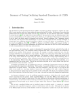
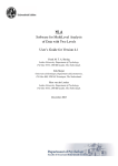
been built and tested at Legnaro [1]. In figure 3.1 the technical drawing and a picture of
the HPWR cap used at Legnaro is shown, mounted at the end of the moving bar. On the
cap there are two spray nozzles from which water comes out at high pressure (100 Bar
max).
Figure 3.1: Picture and technical 3D drawing of the HPWR cap cap rotating inside the cavity. It
goes up and down ejecting water at 100 bar.
The cap rotates along the moving bar vertical axis. Thus the two spray nozzles located
on both side of the cap move so that they can rinse the whole inner surface of the cavity.
Moreover, while the cap is rotating, a mechanism moves the bar along a vertical path to
allow the water jets to scan the entire cavity’s surface. The vertical motion is repeated
many times, changing its direction when the cap is close to one end of the cavity. The
system is designed for 1.3 GHz 9-cells TESLA-type cavity [12] and it can rinse cavity with
a total length of 1256 mm. The minimum beam pipe’s aperture diameter should be at
least 50 mm.
A Visual Basic computer program allows to control the vertical position and the speed
18
High Pressure Water Rinsing
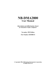
Figure 3.2: Picture of the 3-cell spun niobium cavity mounted on the HPWR system.
3.2 HPWR Protocol
19
of the head very precisely (figure 3.3). In fact, the electrical motor is equipped with a double channel encoder for measuring the rate and the number of steps the shaft makes. And
therefore the computer program gives the possibility also to rinse cavity with a particular
sequence.
A 0.1 µm particle filter, which is located close to the motion system, (working pressure
100 Bar) makes sure that the ultra pure water is free of dust. The cavity at the upper end
is closed by a flange, whereas at the bottom is mounted on a flange. A flow of filtered nitrogen creates a little overpressure inside the cavity to help the water to exit from the four
outlets at the bottom. Typically the rinsing lasts a couple of hours; after that the cavity
is disconnected from the system and brought in a 100 class clean room for the assembly of
the RF antennas and pumping line.
Figure 3.3: Screenshot of the HPWR sofware control panel.
3.2
3.2.1
HPWR Protocol
Preliminary Operations
The HPWR usually comes before the sputtering or the rf test. It is also used to remove
the residual acid from the cavity wall between the EP and the SUBU. After the HPWR
the cavity is left drying in the class 100 clean room and nobody can enter or work in that
20
High Pressure Water Rinsing
room. It always preferable to make sure everything is ready and assembled in the clean
room (cathode or flanges RF and antennas) before the cavity enters.
• If the system has not been used for more than a week it’s always better check its
complete functioning before start using it (the software, the motor, the compressor
and the deionized water plant).
• Warn the people working in the chemistry about the date and time of the process
because it is noisy and uses a lot of deionized water.
• Check that you have the right flanges to connect the cavity to the apparatus. Usually
Copper cavities have standard CF100 flanges.
• Check that you have the upper transparent flange with the nitrogen gas connection.
(See picture 3.4)
• Select the o-ring for the flanges you are using.
• Clean every components.
• Make the needed screws and the tools ready.
• Make the nitrogen gas filter ready.
3.2.2
Cavity mounting
• Make sure the bar is completely down.
• Position the cavity on the system flange.
• Fix the lower flanges with hex socket screws. Just rest on the upper cap on the top
of the cavity.
• Use the computer program (see next section) to check the right range of the bar
motion. The bar should not exceed the cavity height.
3.2.3
Computer program
The program is written with the Visual Basic software and it’s saved in the older
computer of the chemistry.
•
•
•
•
•
•
•
•
•
Switch on the main switch of the HPWR system.
Connect the computer with the HPWR control.
Turn on the switch for the cap rotation on the MPR control.
Check if the cap is rotating.
Switch on the computer.
Open Project c:/vb/hpr/motor1.rnak
Windows - Project - view form or ">"
Press "Zero" to let the bar go to the lowest position.
To adjust the limits insert the lower-end number then PRESS RETURN. Write the
upper-end number than PRESS RETURN. To have an idea of the limit values see
the table 3.1 but perform a check test before starting.
• Press "Start" to run
3.2 HPWR Protocol
21
Figure 3.4: Picture of the copper cavity mounted on the HPWR system.
•
•
•
•
Press "Cycle
select the speed with "+" and "-" buttons (a good speed is 140)
If the motion and the high limits are right close the upper flanges
Write down the lower end and the upper end of the bar range.
Cavity
Lower end
Upper end
Mono-cell (L1 and L2)
210
2541
Three-cell
210
3000
Table 3.1: HPWR bar range limits. Always check the limits before fixing the upper flange!
3.2.4
•
•
•
•
•
•
•
•
Start the process
The bar is cycling up and down and the cap is rotating.
Connect the gas filter.
Connect the nitrogen gas line.
Go to the deionized water box outside the laboratories and open the valve on the
outlet connection of the compressor.
Switch on the compressor
Back to the chemistry open the valve on the wall water pipe.
Start the compressor with the green button on the control box of the compressor.
Wait the time needed for the cleaning procedure.
22
High Pressure Water Rinsing
3.2.5
End the process
• Prepare a large beaker with two centimeters of water in. It must have a diameter
higher than the cavity flange.
• Switch off the compressor with the red button
• Close the the valve on the wall water pipe.
• Disconnect the nitrogen gas line and close the hole on the flange.
• Go to the deionized water box outside the laboratories and switch off the compressor
• Close the valve on the outlet connection of the compressor.
• Open the two valves outside the deionized water box to empty the pipe that connect
the compressor to the HPWR system.
• Back to the chemistry lab.
• Press the "Stop" button on the computer software.
• Press "Zero" and wait the bar going back to the lowest position.
• Unscrew the bottom flange of the cavity.
• To avoid that particles enter in the cavity during transportation to the clean room
set the cavity bottom flange in the beaker.
• Switch off the cap rotation and the main switch of the HPWR system.
• Cover the HPWR flange with a cap.
• Disconnect the cable from the MPR control.
23
Chapter 4
Sputtering of Niobium Thin Film
onto a Copper Cavity
The present section gives an outline of the sputtering system and describes the full
coating procedure for the 1,5 GHz mono-cell cavity.
Each sections will outline the steps to be carried out for a correct mounting on the
sputtering system, the pump down and the bake out, the sputtering, and finally venting
and dismounting.
4.1
The vacuum system
The layout of the vacuum system is given in figure 4.2. The system is described starting
from the exit pipe and it is made up of a double stage Edwards E2M18 rotary pump (RP).
That pump reaches the maximum vacuum of 10−3 mbar and uses the TW Edwards low
vapor tension oil. The rotary pump is closed by an electropneumatic valve, V1, that opens
when the pump is switched-on and closes with the switching off. The system is provided
with an absorption trap (ZT) and and electropneumatic valve to avoid the backstreaming
problem, that means the oil and air reflux from the low vacuum towards the high vacuum
camera. The trap is followed by another valve at VAT angle, V2 that, which is used to
isolate the rotary pump during leak tests.
A sequence of two crosses, situated between the valve V2 and the turbomolecular pump,
complete the low vacuum zone: to one of the crosses is connected the VAT (V3)linear valve
for the leak detection without stopping the pumping; to the other is connected the valve
V4 of the first nitrogen line for the venting of the zone situated behind the gate valve (GT).
The rotors on the turbomolecular pump Seiko Seiki TP300 (TP) make use of magnetic
levitation. Thus, it doesn’t use any oil. The control for the pump system is relatively simple but it doesn’t include an automatic reduction of the pumping speed (Stand-by): this
inconvenience has been overcome, by installing a by-pass (BP) that directly connects the
pump to the chamber through a tombak bellow and a valve (V5) UHV All-Metal Bakeable
Varian, with a very low conductance. Thus, it permits working in the chamber at pressure
24
Sputtering of Niobium Thin Film onto a Copper Cavity
of 10−3 -10−1 mbar during the sputtering stage, keeping the pump at the maximum pumping speed, without damaging it.
The turbo pump doesn’t work if the primary power is interrupted for more than 50ms,
in this case the pump panel makes use of a battery backup system, that supplies the magnetic bearing coils. The slowdown of the pump, in case of blackout, represents a difficult
problem because the pumping stops and, although the system remains sealed and there
are no problems of contaminations, until manually restarted.
Figure 4.1: Picture and drawing of the system used for depositions.
The turbo panel is connected to a controller that is used to open and close of the
gate valve. This panel is programmed in a way that the gate valve opens only when the
pump has reached the maximum speed. This is not a problem if it is possible to reach a
preliminary vacuum in the chamber using the bypass, so when the pumping is switched-on,
the bypass has to be opened. The gate valve remains closed during the acceleration of the
turbo because a good evacuation of the sputtering system has to be very slow; especially
during the phase of viscous flux (1-10−3 mbar), when it is very easy to raise some dust or
particles in the system.
The sputtering chamber was ideally divided into three zones: the base, the cavity and
the cathode. The base is connected to the pumping system through the gate valve and
it is provided with a viewport through which visual monitoring of the plasma is possible.
Several safety valves are placed all along the system and at the bottom of the vacuum
chamber the following pressure gauges are connected:
4.1 The vacuum system
Figure 4.2: Complete structure of the vacuum system.
25
26
Sputtering of Niobium Thin Film onto a Copper Cavity
1. Bayard-Alpert IMR112 Balzers (10−3 -10−8 mbar) BA,
2. Ion Gauge IMR 132 Balzers(10−6 -10−13 mbar) IG,
3. Pirani TPR018 (103 -10−3 mbar) PG,
4. Capacitive CMR264 Pfeiffer(101 -10−4 mbar) CG.
Three gas lines arrive to the base: nitrogen for the venting of the low vacuum area, mixed
oxygen-nitrogen for the venting of the high vacuum chamber, and pure argon for the
sputtering. The oxygen-nitrogen mixture (only used for the latest depositions) enters the
chamber by passing through an all-metal valve (V6): it is used to guarantee a controlled
oxidation of the surface without humidity (H2 O < 1 ppm). The nitrogen, whose pressure
is controlled through a pressure regulator at double stage, enters, through V4, the area
behind the gate valve, while the argon N60 (purity 99,9999%) is "stocked" in a 15l bottle
fixed in the system. The connection between the bottle and the line uses a Cajon system, followed by a all-metal angled valve (V7) and by an all-metal dosing valve precision
valve(V8).
During pumping and baking, the precision valve always remains opened
while the all metal valve that precedes it, is opened only during the sputtering process.
To place a precision valve to regulate the flux of argon at the base of the chamber means
that the most part of the gas is immediately pumped and only a little fraction of gas is
changed with the chamber. In this way, the pressure in the chamber is more stable and,
moreover, the film contamination, due to the gas impurities, is reduced.
4.2
The cathode
The cathode is made of the following parts:
1.
2.
3.
4.
5.
6.
stainless steel liner with a CF100 flange (figure 4.4),
niobium cathode,
upper niobium disc,
lower niobium disc,
flat screw with an hole along the axis,
quartz tube 150mm long. Its diameter is wider than the upper niobium disc because
it should be possible to substitute the quartz in case of break.
The cathode is located on the axis of the system (figure 4.3). It consists of a vacuum tight
stainless steel tube (liner) surrounded by a niobium tube. The niobium tube is a rolled
niobium sheet, welded by the electron beam technique. It has an RRR superior to 250
because a high purity is necessary to reduce the contaminations of the film due to the
cathode.
The liner is welded to a flange CF100 and closed at the base with a TIG welded plate.
It supports the Nb cathode (cathodes of different diameters were used) and the screen of
4.2 The cathode
27
Figure 4.3: Cylindrical Standard Cathode.
quartz; the thermic and electrical contact with the niobium cathode occurs through nine
steel tabs under tension stress that can open or close to increase the diameter of the steel
tube (figure 4.5). The upper and lower niobium discs are screwed to the cathode. The lower
niobium disc is fixed by a flat screw to the steel tube to prevent the falling of the cathode.
The quartz screen avoids the insulator metallization and it was especially useful when the
cathode was sputtered on all the surface at the same time, because in that configuration
the steel tube was sputtered too.
The quartz screen was especially useful when the cathode was sputtered on all the
surface at the same time, because in that configuration sputtering of the steel tube was
more likely. The Niobium cathode is perhaps the most critical part of all the system, for
the concerns of cleanliness. The best place to leave it is the vacuum system itself, with the
pumps running.
4.2.1
The Cathode Assembly
The cathode should be assembled in clean room and all the operators must put clean
room clothes on. Some useful tools are: two wrench n.13, two wrench n.5.5, two wrench
n.7, a Lineman’s pliers.
• Wash the liner, the quartz tube, the niobium discs and the screws in ultrasonic bath.
Dry them with ethanol and flux of nitrogen gas.
• Clean the niobium cathode with tetrachloroethylene, acetone, ethanol.
• Prepare the cathode and all the necessary bolts on the clean room table.
• Screw the upper niobium wing to the niobium cathode.
• Insert the niobium tube on the stainless steel liner, using an hammer with a plastic
head if necessary. The tube is positioned on the liner as in figure 4.3
• Fix the lower niobium disc with the flat screw.
28
Sputtering of Niobium Thin Film onto a Copper Cavity
CF100 fla ng e with
c e ntra l ho le
901,40
60
A
25
TIG we ld ing to the tub e
fo r va c uum se a ling
DETAIL A
DETAIL 2 : 1
Figure 4.4: Technical drawing of the liner.
• Insert the quartz tube in the liner.
• Fix the quartz tube from falling down.
• Insert the CF100 ceramic insulator and fix it to the liner flange with screws. Remember the copper gasket!
• Remember to use three long screws in order to fix the eyebolts to the upper flange
of the cathode. The eyebolts are useful for the cathode lifting with the crane as in
figure ??.
• Screw three eyebolts to the flange.
• Insert and fix the stainless steel chamber after the ceramic insulator as in figure 4.6.
4.2.2
The bias grid components
In addition to the cathode described before, the biased cathode has some more components:
1.
2.
3.
4.
5.
6.
7.
six niobium rods 600mm long and 3mm of diameter.
Six stainless steel springs 20mm long.
Nuts for 3mm screws.
Washer for 3mm screws.
Six ceramic cylindrical insulators with cap (figure 4.8a).
Six American screws for the ceramic insulators.
Six Socket screws, also known as Allen head, for the ceramic insulators. They are
4.2 The cathode
29
Figure 4.5: Detail of the steel tabs built up to guarantee a good electric contact between the
stainless steel tube and the Niobium target.
8.
9.
10.
11.
12.
13.
fastened with a hex Allen wrench.
The upper niobium disc has three threaded close ended holes for the insulator connection.
The lower niobium disc has three threaded close ended holes for the insulator connection (figure 4.8c).
Upper stainless steel disc: divided in two half-moon parts. They are connected with
two strips as in figure 4.9.
Lower stainless steel disc (figure 4.8c)
One nut for a 3mm screw plum welded to a washer as in figure 4.7.
Ceramic CF16 feedthrough (figure 4.6).
This is the most efficient grid configuration with niobium rods. The niobium tube is
surrounded by six vertical rods isolated from the cathode by ceramic cylinders (figure
4.8a). Six springs stretch the bars in spite of the thermic extension.
30
Sputtering of Niobium Thin Film onto a Copper Cavity
Figure 4.6: The ceramic insulator is connected to a stainless steel chamber. On the left a detail
of the bias feedthrough.
Figure 4.7: Detail of the electrical connection between the grid and the feedthrough.
4.2 The cathode
4.2.3
31
The bias grid assembly
• Wash the liner, the quartz tube, the niobium rods, the washer, the nuts, the springs,
the niobium and SS discs, the screws in ultrasonic bath. Dry them with ethanol and
flux of nitrogen gas.
• Clean the niobium cathode, the ceramic insulators and the feedthrough with tetrachloroethylene, acetone, ethanol.
• Prepare the cathode and all the necessary bolts on the clean room table.
• Screw the upper niobium wing to the niobium cathode.
• Insert the niobium tube on the stainless steel liner, using an hammer with a plastic
head if necessary. The tube is positioned on the bottom of the liner as in figure 4.8a.
• Fix the lower niobium disc with the flat screw.
• Insert the quartz tube in the liner.
• Screw the ceramic insulators to the niobium discs with the Allen head screws. The
insulator caps should face the niobium disc as in figure ??.
Figure 4.8: Details of the bias grid: a)The springs and the ceramic cylindrical insulators with
cap. b) 3D drawings of the grid connection to the cathode. c)The disc assembly mounted on the
cathode. e)Bottom view of the cathode during sputtering.
• Fix the two half-moon SS disc parts to the upper niobium disc. They are kept fixed
with two strips below (as in figure 4.9) and two strips above.
• Screw one nut to each niobium rod then insert them in the respective holes of the
upper SS disc.
• Remember to insert the two strip of the upper disc.
32
Sputtering of Niobium Thin Film onto a Copper Cavity
Figure 4.9: Grid with niobium rods with springs to keep them tight.
Figure 4.10: The copper cavity on its seat.
4.2 The cathode
33
• IMPORTANT. All the rods should merge from the disc just enough to fix them with
one nut. All rods except one! This one should emerge enough to be fixed with the nut
and leave some thread left. In that rod the electrical connection for the feedthrough
is fixed with another nut as in figure 4.7.
• Insert the two strips on the top and then fix each rod with a second nut on the top.
• Screw one nut to each niobium rod end, insert the SS lower disc and fix it to the
insulators on the bottom of the cathode.
• Fix the lower SS disc to the insulators with the screws.
• Insert the springs and the washer to each rod end and fix it with a nut.
• Make sure every rod is stretched and doesn’t touch the cathode.
• Check all the connections with the multimeter in the continuity mode.
• Insert the CF100 ceramic insulator and fix it to the liner flange with screws. Remember the copper gasket!
• Remember to use three long screws in order to fix the eyebolts to the upper flange
of the cathode. The eyebolts are useful for the cathode lifting with the crane as in
figure 4.14.
• Screw three eyebolts to the flange.
• Insert the stainless steel chamber after the ceramic insulator. Make sure the CF16
aperture on the chamber side faces the nut for electrical connection.
• Screw the feedthrough to the nut. (Remember the gasket!) Close the flanges with
screws.
• Check again all the connections with the multimeter in the continuity mode.
4.2.4
The Cathode insertion
• This procedure needs two operators working in the clean room.
• Set slowly the cavity on its seat, as in figure 4.10.
• Keep the cathode horizontal, coaxial with the cavity. Make sure you have enough
space on the table.
• Insert the CF100 gasket on the cathode.
• One operator look inside the cavity and moves it towards the cathode.
• Make sure not to scratch the cavity wall during the introduction. The cathode should
be always coaxial with the cavity.
• When the two flanges are touching, fix it with the screws.
• Tight all the screws.
• Close the assembly with a plastic bag free of dust.
• The small clean room has no crane, so it’s necessary to exit the cathode by hand.
This operation requires a lot of care and some muscular strength.
• Take the assembly out of the clean room and hang it to the crane.
34
Sputtering of Niobium Thin Film onto a Copper Cavity
4.2.5
•
•
•
•
•
The cavity placement on the system
Lift the assembly on the top of the vacuum system flange.
When the assembly is on axis with the flange remove the plastic bag slowly.
Remove the cap from the flange and put the gasket.
Connect the flanges with the screws and tight them.
Mount the retaining stainless steel rods around the cavity to prevent its collapse
(figure 4.13).
4.3
The Pump down
The pump down from atmospheric pressure to the molecular regime (10−2 mbar) has to
be very slow in order to avoid turbulence in the cavity, which can transport dust: two hours
are considered adequate. For the valves name and the other components of the system we
refer to the scheme 4.2.
4.3.1
The Pump down procedure
• The system is initially in the following condition: the turbo pump is off, the gate is
closed, the rotary pump is running and valve V6 is closed.
– the pumps are off,
– every vane is vented,
– the gate is closed.
•
•
•
•
•
•
•
•
•
•
•
•
Switch on the Rotative pump.
Open V2.
Switch on the Turbo pump.
Open V5 a bit and then wait the pressure on the HP goes down.
Open V6 and V8 slowly.
Open V5 a bit and then wait the pressure on the HP goes down. Repeat this
operation.
Wait the pressure stabilized below 10−4 mbar and the turbo pump reaches its maximum speed.
Open the gate valve GT.
CLOSE the valve V5.
When the pressure stabilized below 10−5 mbar switch on the Ion Gauge IG.
Wait the pressure stabilizes below 10−7 mbar before starting the baking. It may takes
more than two hours.
Perform a leak check.
4.4 The baking system
4.4
35
The baking system
To heat the system, every flange and the cavity body are tightly surrounded by heating
collar. The heating process is controlled by two "UHV BAKING CONTROL" heating
boxes.
Each heating box controls and regulates the temperature of three zones of the system
with three heating units. A digital timer allows to set the process time. The collars are
supply, through the box, with 220V and controlled with Resistance Temperature Detectors
(RTDs).
Figure 4.11: Front panel of the "UHV BAKING CONTROL" heating box.
Each heating unit allows to set the zone temperature and the maximum temperature
(Alarm) one zone could reach before the heating process is shut down. The electrical
connection are all in the heating box rear panel.
The system is divided into seven zones. Each zone temperature is monitored with one
temperature sensor positioned in a strategic place.
Most of the system elements are made of stainless steel and tolerate temperature till
◦
300 C. On the other side the ceramic insulator is sensitive to temperature gradient and
should be heated slowly and homogeneously until 150◦ C. The gate has a viton viton o-ring.
and its maximum baking temperature is 120◦ C. The turbopump heater is independent and
regulate by the pump control unit. The electronic placed on the pump is cooled by a fan.
The seven zones are:
1.
2.
3.
4.
5.
6.
7.
The
The
The
The
The
The
The
cathode and the ceramic insulator flange
cavity and its flanges.
gate.
CF35 gauge flanges and the CF16 all-metal valve flanges.
chamber placed between the gate and the cavity.
by-pass chamber, its bellow and the CF16 flanges.
turbomolecular pump.
36
Sputtering of Niobium Thin Film onto a Copper Cavity
Table 4.1 suggests a possible temperature set.
Zone
Temperature (◦ C)
1
Cathode
150
2
Cavity
150
3
Gate
100
4
Gauges and CF35 flanges
150
5
Pre-chamber
150
Bypass
150
Turbomolecular Pump
120
7
Table 4.1: Standard baking temperature set for every zone.
Take care to avoid cold spots during baking, which could affect the final vacuum.
Moreover, in case of power failure during baking, the gate would close and the pressure
would rise in the hot system, opening the way to the formation of not well defined oxides
on the cavity surface. It seems that for copper cavities this oxidation doesn’t affect the
final results.
Under the baking box there is the multifunction box (figure 4.12): on the right side
there is a control unit for fans system and heating collars. This units allows to control
the cavity temperature during coating. The temperature is measured by a thermocouple;
when it exceeds the set temperature the heating collar are switched off and the fan are
switched on.
On the left side of the multifunction box there is splitter for the nitrogen line. One line
goes to the nitrogen gas gun and the other line pass through a pressure reducer and goes
to the venting valve.
Figure 4.12: Multifunction box: from the front panel the operator can set an additional baking
units and he can also regulate the nitrogen gas pressure. In the rear panel there are two sockets
for the heating collar or the cooling fan plugs. One thermocouple is connected to the heating unit.
4.5 The magnet assembly and the cooling system
4.4.1
37
The baking procedure
• While the cavity pressure goes down to 10−7 mbar, mount the heating collar around
the cavity as in figure 4.13.
• Check the RTDs functioning and fix one on the cavity cell. Each temperature sensor
is connected to the relative zone. Be sure to pick up the right one.
• Mount the respective heating collar around the top and bottom flanges of the cavity.
• Mount the heating collar around the ceramic insulator flanges.
• Fix the respective temperature sensor on the ceramic insulator flange.
• Check all the other RTDs and heating collar already mounted on the system. Be
sure no cables touch them.
• Wrap the cavity with aluminium foil to improve the temperature uniformity.
• Notes the pressure and Switch off the IG.
• Set the baking time on the heating box.
• Set the alarm temperature on the heating box.
• Set the temperature of each zone on the system on the heating box. The heating
should be slow so increase the temperature in steps of 10◦ C about every 15 minutes
until the maximum temperature for each zone is reached (See table 4.1 for suggestion). The pressure should not exceed 10−5 mbar.
• Wait the baking time
• When the baking shut down, after the set time, wait the system cooling down naturally.
• Switch on the IG.
• If all these steps have been carried out correctly, the vacuum level should be 10−9 mbar
or less.
• Remove the collars on the top of the system, except the cavity ones.
4.5
The magnet assembly and the cooling system
A Nd-Fe-B magnet is kept between two little iron circles that concentrate the magnetic
field lines. The whole assembly of magnets and irons are fixed on a stainless steel tube of
9mm diameter that assure the movements up and down inside the liner (figure 4.3). The
magnet and the bar assembly movements inside the cathode occurs through an electromechanic actuator mounted on the side of the sputtering camera. It is controlled remotely
and it moves at a user controlled speed. In order to know the magnet position, a dashboard
that reproduces the shape of the cavity is mounted on the top of the system. To avoid a
current flow from the cathode liner walls, through the magnet to the actuator, the magnet
is isolated from the moving 9mm diameter bar.
During the sputtering the cathode is subjected to an ionic bombardment and can reach
temperatures of 1000-1500◦ C as the power increases. To avoid the overcoming of the
temperature of demagnetization, the Curie temperature, which is 80 ◦ C, it is important
38
Sputtering of Niobium Thin Film onto a Copper Cavity
Figure 4.13: Preparation of the cavity baking. The heating collars, the temperature sensor and
the retaining bars.
that the magnet inside the cathode is efficiently cooled during sputtering. Currently the
magnetron cathode is cooled by a water closed circuit system: the water flows down through
the tube that supports the magnet; then it flows back inside the stainless steel tube and
goes out through the aperture above the cathode flange as shown in figure 4.14.
4.5.1
Set the cooling system
• Mount the magnet and the bar assembly on the actuator and check in which position
the magnet is leveled with the cell.
• Adjust the dashboard height.
• Insert the magnet in the liner and screw the cap with teflon.
• Fix the bar assembly on the actuator.
• Control the magnet rotation and movement inside the liner.
• Connect the water tube to the liner output.
• Connect the other water tube to the input fast connection on the top of the liner.
• Check if the water circuit is sealed well.
• Fix the plastic cap and the plastic bellow to avoid accidental contact with high
voltage.
4.5 The magnet assembly and the cooling system
39
Figure 4.14: The cathode and the magnet are cooled by a water closed circuit and the water flows
through the tube that sustains the magnet to the stainless steel tube.
40
Sputtering of Niobium Thin Film onto a Copper Cavity
4.6
Sputtering
The starting point of the sputtering work was the CERN standard procedure (Figure
4.15).
Figure 4.15: Simplified structure of the standard CERN configuration for sputtering niobium into
1,5 GHz copper cavities.
The sputtering deposition is performed in many steps: the magnet is shifted along
the cathode length, to the end of uniformly cover the internal surface. One single step is
adopted for the deposition in the cell, with the magnet in the central position. Two sets
of sputtering parameters are employed, one for the cut off tubes and another for the cell.
In the Cylindrical Magnetron (CM) configuration the standard procedure is:
“the extension tubes are coated first in an argon atmosphere of 1x10−2 mbar; a stable current of 1A is set between the cathode and the grounded sample holders. The magnet is
moved in 14 steps over the cathode length in order to coat each tube uniformly. The cell
is coated with slightly different discharge parameters, leaving the magnet fixed in its center
for 15 minutes: the argon pressure is reduced to 1.5x10−3 mbar so as to increase the mean
free path of the atoms ejected from the cathode and the current is increased to 3A (400V)
to rise the sputtering rate.”[9]
4.6.1
Sputtering Procedure
• Set cavity temp on the multifunction box to 150◦ C (figure 4.12).
• Position the temperauture sensor of the multifunction box on the cavity cell.
• Connect the fans to the multifunction box (COOLING socket).
4.6 Sputtering
•
•
•
•
•
•
•
•
41
Connect the white socket box to the multifunction box (HEATING socket).
Connect the three heating collar of the cavity to the white socket box.
Set the electrical connection with the power supplies Figure 4.16 and 4.17
Open the exit and then the inlet valve for the water cooling circuit. They are on the
wall near the blue gas cabinet.
Switch on the heating on the multifunction box.
Switch on the cooling on the multifunction box.
Press start on the multifunction box.
Wait the temperature stabilizes.
Figure 4.16: Schematic of two electric circuits to connect the cavity, the cathode and the biased
grid. A and B are conceptually the same although the currents distributed by the power supplies
are different.
42
Sputtering of Niobium Thin Film onto a Copper Cavity
Figure 4.17: Schematic of the electric circuit for connecting the pulsing device between the power
supply and the cathode.
•
•
•
•
•
•
•
•
•
•
•
•
•
•
•
•
•
•
Open the bypass valve.
Close the gate.
Wait the pressure stabilizes.
Close the argon line leak valve.
Open the all-metal valve.
Slowly open the argon leak valve to rise the pressure up to 5x10−5 mbar.
Switch off the Ion Gauge.
Increase the argon pressure to 4x10−3 mabar.
Move the magnet to the top position. Over the cavity top flange.
Set the sputtering current to 1A.
Set the bias voltage to 100V.
Set the actuator speed to 3/4 for both the Up and Down direction.
Move the magnet down below the bottom flange of the cavity and then up again,
two times (Ramonage).
Leave the discharge in the top position (over the upper flange of the cavity), for two
minutes (gettering of residual impurities).
Leave the discharge in the low position (under the lower flange of the cavity), for two
minutes (gettering of residual impurities).
Don’t turn the discharge off.
Start the deposition from the top flange (Pos. 20), The sputtering parameters for
the cut off tubes are the following: pressure 4x10−3 mbar, Current 3A, time for each
step 1 min 40 s. The total number of steps for each tube is 14. The voltage of course
will float, having fixed the current, but it should remain above 400 V.
Repeat the same procedure in the lower tube, starting from the bottom flange and
4.7 Tips to remember for a good sputtering procedure.
•
•
•
•
•
•
•
43
moving towards the cell.
Place the magnet in the central position The sputtering parameters for the cell are
the following: pressure: 4x10−3 mbar, current 5A, time 20 min.
The temperature of the cavity will continue to oscillate triggered by the power input
from the plasma and the heaters, and controlled by the cooling action of the fans.
This oscillation can be maintained within 5o C.
When the deposition in the central cell is finished, turn the power supplies off.
Close the argon line leak valve.
Wait the pressure goes below 10−4 mbar and open the gate valve.
Set the heaters to room temperature and allow the cavity cool down.
Disconnect the power supplies.
4.7
Tips to remember for a good sputtering procedure.
You should remember to:
1. Do not move undesired particulate and dust during the cavity pumping start up.
2. Avoid a sudden baking to high temperature (it is preferable to increase temperature
at steps of 10-20 C looking constantly at the chamber pressure.
3. Avoid any inhomogeneity in temperature distribution during baking.
4. The baking time should be at least 24 hours.
5. Open the argon valve step by step in order to avoid a sudden venting and dust
floating.
6. Check that the cavity temperature is uniform during the sputtering.
7. Check the electrical contacts, mostly the cathode one.
8. Never vent the cavity when it is hot or at a temperature higher than 40◦ C.
9. Vent slowly to avoid dust motion into the cavity.
10. Avoid any contact of the cathode with the cavity during the cathode insertion and
extraction .
4.7.1
•
•
•
•
•
•
•
•
•
•
Process Shut Down and System Opening
When the cavity is at room temperature close the water circuit.
Disconnect all the electric cables.
Empty the water circuit tubes.
Remove the magnet system.
Remove the fans and the heating collar.
Close the gate.
Close the by-pass valve.
Switch off the pumps and wait the turbopump stops.
Open the venting valve V4.
Close the leak valve V6 on the "dry air" gas line.
44
Sputtering of Niobium Thin Film onto a Copper Cavity
•
•
•
•
•
•
•
•
•
•
•
•
•
•
Open the all-metal valve V9 in the "dry air" gas line.
Open slowly valve V6.
Fill the cavity with a small overpressure.
Close all the valves of the two venting lines.
Mount the eyebolts on the top flange of the assembly and fix them to the crane.
Wear the clean room clothes.
Loosen up the screws of the top flange.
Disconnect the bottom flange.
Bring the cavity and the cathode to the clean room
This procedure needs two operators working in the clean room.
Set slowly the assembly on its seat.
Remove the screws from the cavity top flange.
One operator look inside the cavity and moves it away from the cathode.
Make sure not to scratch the cavity wall during the extraction. The cathode should
be always coaxial with the cavity.
• Close the cathode with a plastic bag free of dust.
• Bring the cavity to the HPWR system.
45
Chapter 5
Cryogenic apparatus and cavity
stand
During the test, the cavity has to be cooled at cryogenic temperatures in order to
reach the superconducting state. The transition temperature for Nb is 9,2K. The systems
are typically operated at sub atmospheric temperatures in order to better simulate actual
accelerator operating conditions.
5.1
The cryogenic laboratory
In the rf testing facility there are four apertures which can host a cryostat. Three of
them are used to test QWRs and single cell TESLA type cavity. This kind of cryostat
can hold 100 liters of helium. The last one is for the multicells TESLA type cavity with a
volume of 400 liters of helium. This cryostat has been designed for operating at 4.2K and
1.8K with a maximum power of 70 W.
The helium vessel is constituted by three successive chambers containing respectively
helium gas or vacuum, liquid nitrogen, the inner being under vacuum to thermally insulate
the sides. The second chamber (starting from the outside) is connect to the liquid nitrogen tank placed outside the laboratory(see figure 5.6). At the top, thermal insulation is
improved by several copper screens cooled with the recovery helium cold gas. The cryostat
with the cryogenic insert with a mono-cell cavity is shown in figure 5.1.
In order to reduce the cooling cost, a preliminary cooling is achieved by using the
liquid nitrogen of the second chamber. Thus the He vessel is filled with Helium gas at
a pressure of 1000mBar, and a thermal contact is created between the He vessel and the
liquid N2 chamber by filling the chamber in the middle with He gas at 200mBar. Once
the temperature reaches 80K, the He gas is removed from the intermediate vessel and the
transfer of liquid He at 4.2K into the main vessel is started. The transfer does not stop
until the liquid level reaches 1000 or 1400 mm, depending on the cavity size.
The cavity is tested at 4.2K and then at 1.8K. The temperature of liquid helium can
be lowered decreasing the chamber pressure. A pumping line takes away the vapour over
46
Cryogenic apparatus and cavity stand
Figure 5.1: Cryogenic insert designed to hold a 9-cells cavity.
5.1 The cryogenic laboratory
47
the liquid and hence some liquid helium evaporates to compensate the drop of pressure.
Furthermore, a liquid helium supply at 1.8K must be introduced in order to keep the level
constant. This task is carried out by a heat exchanger, that utilize the cooling capacity
of the return gas stream to cool down the incoming liquid. The cooled fluid is sent into a
liquid/gas separator. The low temperature portion is taken apart by a sinter brass plate in
the middle of the separator. The liquid flows by capillarity action towards the lower side
while the gaseous phase remains on the upper part and it is used to refrigerate the copper
screen. The stream of liquid is regulated by two valves which can be operated manually
from the outside. By changing the pumping speed it is possible to set the evaporation rate
and, in turn, the amount of power removed from the dewar. The pressure and thus the
temperature, of the bath is regulated by controlling the system pumping speed.
Figure 5.2: Plot of the pumping speed as a function of the temperature for different power
dissipated. The labels on the right refer to the pumps illustrated in figure 5.3
Typically, a single cell cavity dissipates only few tens of watts during the test. The
rf tests are performed at 4.2K and at 1.8K with the result of making the pumping speed
range very large as it is shown in figure 5.2. This plot illustrates the pumping speed needed
to remove a given power as a function of the temperature of the liquid helium.
Figure 5.3 is a schematic of the pumping configuration. By using different combination
of pumps, namely RA3001, SV1200, SV200, SV25 which work at different speed ranges, one
is able to cover a wide range of pumping speed requirements. The first pump is a Roots
48
Cryogenic apparatus and cavity stand
pump while the others are rotating pumps. The operator can set the pumping control
system up with the working pressure in the cryostat in a range between 16 and 1000mBar.
The system initially tries to pump the cryostat with the smallest pump (SV25). If the
selected pressure is not reached, a larger pump (SV200) is automatically activated. In case
that also this one cannot attain the selected pressure, also the third pump (SV1200) is
activated. If an adequate pumping speed is still not achieved, at 40mbar the Roots pump
(RA3001) starts.
Figure 5.3: Arrangement of the cryostat pumping system.
Along the pumping line there are several sensors connected to the automatic control
device. The pressure control (PC) automatically opens the three valves VR1, VR2, VR3
to select the working point of the pumps. In addition, each rotating pump can be excluded
from the line by the intercepting valve that precede them. There is also a gas cooler in
the line, because the Roots tends to be damaged by the hot gas present at the exit of the
pump itself. At the exit of the pumping line, the helium gas is stored and when the tank
is full it is sent to the liquefier.
The purpose of a cryogenic system is to generate and maintain very low temperatures
and a suitable network of temperature sensors and heaters is needed. The temperature
monitoring system in the cryostat is undertaken by three kinds of sensors: diode thermometers, carbon glass resistor and germanium resistance thermometers. The diodes are
ALSO used as an additional level probe, while the carbon glass and germanium sensor are
employed for the temperature region between 4,2 and 1,8 K.
After the preliminary evacuation, the cavity is mounted on the vacuum system for the
5.1 The cryogenic laboratory
49
cold test. The layout of this system is sketched in figure 5.4. Staring from the exhaust
line, there is an oil free backing pump and a turbo-molecular pump. Valve V5 is used to
insulate the turbo in case of power failure. V6 is used in the event that a leak detection
is necessary. V4 is the main gate valve. V7 allows venting the system, with the gate valve
closed. V8 and V9 are for the helium conditioning. V3 allows leaving under vacuum the
"fixed" part of the system, which is connected to the cavity by the VCR between V2 and
V3.
The cryostat vacuum chamber has a long pipe connecting the pumps, at room temperature, to the cavity immersed in the liquid helium. In this situation the cavity itself
acts as a cryogenic pump, while the low conductance of the pipe reduces the effective
pumping speed of the upper pumps. It is thus advisable to evacuate the cavity before
the mounting on the cryostat insert. This job is done by means of a separated vacuum facility. The cavity is pumped leaving it on the movable support used for the chemistry stage.
Figure 5.4: Sketch of the cavity pumping system when it is mounted on the cryogenic stand.
We prefer to carry out baking at low temperatures (less than 100 ◦ C) in order not
to affect the surface properties that were obtained during the sputtering process. After
overnight baking and 8 hours of pumping the pressure is usually in the high 10−9 mbar
range.
50
Cryogenic apparatus and cavity stand
Figure 5.5: Global view of the cryostat pumping system and gas lines.
5.1 The cryogenic laboratory
51
Figure 5.6: The local lines for liquid nitrogen and helium. Both are connected to the system and
monitored by a control panel located in the laboratory.
52
Cryogenic apparatus and cavity stand
5.2
Cavity preparation and mounting on the stand
The cavity arrives in the clean room still wet due to the HPWR. Let the cavity dry in
the clean room before assembly the flanges.
The coupler and pickup flanges are stored in the small clean room cabinet. They should
be cleaned with the special tissue and ethyl alcohol, and checked against possible shortcuts.
The coupler is particularly delicate: it is a copper tube screwed to the rf connector. It
can be easily damaged by attempts to adjust coaxiality of the antenna. These attempts
should not go beyond the necessary preventing of shortcuts. The pickup antenna is much
smaller than the coupler one, and easily removable. Check that it is present before closing
the cavity!
Remember that even the smallest dust particle left on the coupler bellow can compromise the measurement. After the cavity has been equipped with the two flanges with the
measuring antennas, it is ready to be mounted on the cryostat insert for the rf test.
5.2.1
•
•
•
•
•
•
•
•
•
•
•
•
•
•
•
Fix the bellow on the coupler flange (see figure 5.7 for the final assembly).
Set the CF35 zero-length flange on the bellow.
Set the rf feedthrough to the CF35 zero-length flange. Use
Mount the four bars of the movable structure and insert the structure on them.
Check that the holes of the movable structure are aligned with the screw of the
feedthrough CF16 flange.
Fix all the screws and the movable structure.
Screw the antenna on the feedthrough.
Fix the all-metal CF35 valve on the pickup flange (see figure 5.8 for the final assembly).
Close the cajon flange of the pickup feedthrough.
Screw the pickup antenna to the feedthrough.
Check eventual shortcuts and adjust the antennas position.
Fix the pickup flange on the support structure.
Bring the cavity on it slowly and close the bottom flange.
Bring the top flange on the cavity slowly.
Close the coupler flange.
5.2.2
•
•
•
•
Coupler and pickup flange
Mount the cavity on the cryogenic insert
Bring the cavity to the cryogenic lab. The pickup flange on the bottom.
Orient the cavity valve towards the pumping line of the cryogenic insert.
Lift the cavity and fix its top flange on the cryogenic insert disc.
Connect the movable structure of the coupler to the linear feedthrough on the center
of the stand.
5.2 Cavity preparation and mounting on the stand
53
Figure 5.7: The coupler flange when the cavity is already mounted on the stand.
• During this operation the pumping line of the cryogenic stand is pumped dynamically.
5.2.3
•
•
•
•
•
•
•
•
•
•
Close the gate.
Switch off the gauge.
Stop the turbopump and the scroll pump. Wait the turbo stops.
Connect the nitrogen line to the leak valve of the venting line.
Open the nitrogen gas line.
Open the all-metal valve of the venting line.
Slowly open the leak valve and wait the complete venting of the system.
Connect the cavity valve to the pumping line valve on the bottom of the stand.
Close the nitrogen line.
Disconnect the nitrogen line.
5.2.4
•
•
•
•
Venting of the stand pumping line
Cavity pump down
Vent the turbopump.
Switch on the scroll.
Switch on the turbopump and open the gate immediately.
Open the all-metal valve of the pumping line.
54
Cryogenic apparatus and cavity stand
Figure 5.8: The pickup flange. The all-metal CF35 valve is connected to the other pumping line
valve.
5.3 Set the thermometers and the resistances
•
•
•
•
55
Wait the pressure goes below 10−3 mbar.
Open the cavity valve slowly and wait the pressure stabilize.
When the pressure goes below 10−4 mbar open the cavity valve completely.
Perform a leak check.
5.2.5
Cavity baking
• Mount the heating collars around the cavity.
• Insert the temperature sensor on the cell position.
• Connect the heating collars to the socket box of the baking unit. Check that the
socket box and the temperature sensor has the same number.
• Set the baking temperature (150◦ C)
• Switch on the baking unit.
• Switch off the baking unit after the scheduled baking time.
• Wait the cavity cool down. The pressure should reach 10−9 mbar.
• Remove the heating collars and the temperature sensor.
5.3
Set the thermometers and the resistances
• Check that the thermometers work.
• Fix the thermometers as indicated in table 5.1.
• To grant a good thermal contact put some grease between the cavity and the thermometer.
• Warm rf test of the cavity.
• Note the warm critical coupling position of the antenna.
• Screw tightly the rf cable to the cavity rf feedthroughs.
Plug
Control Board
Thermometer code or type
Position
1
LS234D n.3
Cylindrical shaped carbon glass (3)
Cryostat big pumping tube
2
LS208 n.3
Silicon (22)
2nd copper stand shield
2
LS208 n.4
Silicon (89)
1st copper stand shield
2
LS208 n.5
Silicon (87)
Bellow for the coupler
1
LS234D n.1
carbon glass C17497
Cavity cell
1
LS208 n.2
D81068
Beam tube superior
1
LS208 n.1
D66036 (5)
Beam tube inferior
Table 5.1: Thermometers position on the cryogenic insert.
5.4
Stand insertion
• Close the gate valve.
56
Cryogenic apparatus and cavity stand
•
•
•
•
•
•
•
•
•
•
•
•
•
•
•
•
•
•
•
•
•
•
•
•
•
•
•
•
•
•
•
•
•
•
Switch off the turbopump and the scroll pump.
Close the valve on the back of the turbo.
Disconnect the bellows from the turbopump.
Close the bellow and the valve with plastic caps.
Close the compressed air for the system gate.
Disconnect the compressed air line from the gate valve.
Disconnect the gauge cable.
Disconnect the turbopump cables.
Disconnect the rf cables and all the other cables connected to the cryogenic insert.
Take the proper support with the crane and bring it on the top of the stand.
Check that the eyebolts are well screwed to the cryogenic insert top plate.
Connect the snaplinks to the eyebolts of the cryogenic insert top plate.
Remove the top flange of the cryostat.
Check the o-ring and clean it.
Check that the two flanges of the cryostat recovery line and the two flanges of the
cryostat pumping line are closed with a plastic cap.
Use the crane to lift slowly the stand and bring it to the top of the cryostat.
Center the stand and orient its pumping lines (the weight over the cryostat pumping
line big port. There is an X near the right eyebolt).
Insert the stand into the cryostat slowly. Ce careful: the cryostat has a reduction in
the middle of it.
When the flange is nearly closed put some screws in order to center the screw holes.
Close the cryostat and fix the screws. Use socket screws and tight the flange with
the nuts.
Disconnect the snaplinks of the crane from the eyebolts.
Connect the scroll pump to the turbopump with a bellow.
Connect the turbopump cables.
Connect the compressed air line from the gate valve.
Open the compressed air for the system gate.
Connect the gauge cable and check that the pressure is below 10−4 mbar.
Switch on the scroll pump .
Open the valve on the back of the turbo.
Switch on the turbopump and wait for its maximum speed.
Open the gate valve.
Connect the rf cable and perform a warm rf test to check that everything is working
fine.
Close the flanges of the cryostat recovery line using a copper gasket.
Close the flanges of the cryostat pumping line using a viton o-ring.
Check that the gas and cryogenic liquid line cabinet: the valve V4 should be open
and the V3 should be closed.
5.5 Cryostat and auxiliary system preparation
5.5
•
•
•
•
•
•
•
•
57
Cryostat and auxiliary system preparation
Connect the two thermometer cable.
Connect the cryostat gauges.
Connect the antenna step motor cable.
Wrap the helium recovery line with heating tape and connect them to the baking
unit. Set 20◦ C.
Connect the all metal valve of the helium gas recovery line to the membrane pump
with a bellow. Check that the all metal valve is closed.
Switch on the GUARD and the CHART softwares (see chapter 6.1) and check that
all sensors are monitored (if connected): cavity pressure (2 gauges), cryostat pressure
(2gauges), cryostat helium level, tank helium level, temperatures (7 sensors), Radiation monitors (3 monitors), cryostat pumping line pressure, cryostat shields pressure
(2 gauges).
Check that the computers are connected to the network.
Open the needle valve for the helium transfer at 4.2K and 1.8K.
5.6
Shields pump down and cryostat purging
• Switch on the pumping systems of the cryostat shields. To obtain a better vacuum
it is possible to perform this step before mounting the cavity on the stand.
• Connect the big white rotative pump to the cryostat purging line.
• Close the cryostat helium recovery line.
• Switch on the rotative pump.
• Open the valve on the rotative pump system.
• Slowly open the cryostat valve.
• Wait the pressure goes down to 10−2 mbar (30 minutes).
• Close the cryostat valve.
• Open slowly the cryostat helium recovery line to vent the vessel.
• Repeat the procedure three times.
• Switch off the rotative pump and close its valve.
• Disconnect the rotative pump and move it.
5.7
5.7.1
Cryostat cool down
Liquid nitrogen cool down
• Connect the liquid nitrogen inlet and recovery lines to the cryostat.
• Connect the electrovalve, positioned on the nitrogen gas exchanger box, to the nitrogen level control.
• Connect the level sensor to the nitrogen level control board.
58
Cryogenic apparatus and cavity stand
• Turn the red switch, positioned below the nitrogen gas exchanger box, on the ON
position.
• Wait the liquid nitrogen line temperature is below -150◦ C. You can read it on the
gas and cryogenic liquid line cabinet.
• Insert one section (CRIOSTATO) of the helium transfer line in the transfer aperture
of the cryostat. Don’t use any extension here.
• Open the inlet valve of the liquid nitrogen line. Keep the pressure of the shield below
2bar.
• Wait the complete shield filling (green light for "level haut" on the nitrogen level
control board.
• The nitrogen level control board keeps the nitrogen level constant.
• To save nitrogen it’s possible to close the nitrogen filling at that step and restore the
liquid level the day after.
• Switch off the internal shield pumping system.
• Switch off the pressure gauge of the internal shield.
• Open the helium gas line and set the pressure to 100mbar.
• Purge the line.
• Connect the helium gas line to the internal shield valve.
• Open gently the valve and wait until the pressure rise of 200mbar.
• Close the valve.
• Close the he gas line.
• Disconnect the gas line from the internal shield valve.
• Wait the cavity cools down to 80K (usually it takes 6 hours so it is left cooling during
nightime)
• Pump the internal shield.
• Close the inlet valve of the liquid nitrogen line.
• Turn the red switch below the nitrogen gas exchanger box on the OFF position.
5.7.2
•
•
•
•
•
•
•
•
•
Liquid helium cool down
Insert the helium level sensor on the helium tank and connect it to its control box.
Insert the helium level sensor on the cryostat and connect it to its control box.
Bring the helium tank near the cryostat.
Close the helium tank recovery line.
Connect the extension to the transfer line and purge it with helium gas.
Insert the transfer line into the tank, and sustain it with the crane.
Wait the helium flux on the other side become continuous.
Connect the transfer line to its section on the cryostat.
Connect the helium gas line to the helium tank, open the valve and pressurize that
tank (maximum 200mbar).
• Close the needle valve for the helium transfer at 1.8K, on the top of the cryostat.
• Switch on the small membrane pump and slightly open the all metal valve for cooling
5.7 Cryostat cool down
•
•
•
•
•
the cryostat copper shields.
Close the all metal valve when the temperature of the shield is below 40K.
Wait the helium level rise up (800mm).
Close the needle valve for the helium transfer at 4.2K partially to maintain the he
level fixed.
Start the evacuation procedure and the rf measure.
To stop the transfer just close the helium gas line and open the recovery line of the
helium tank. Don’t remove the transfer line.
5.7.3
•
•
•
•
•
•
•
59
Superfluid helium cool down
Restore the helium level of 1000mm.
Depressurize the helium tank.
Close the helium recovery line of the cryostat.
Open the steering-wheel valve on the cryostat pumping line.
Switch on the cryostat pumping line control board.
Open the V3 valve on the gas and cryogenic liquid line cabinet.
Close the needle valve for the transfer at 4.2K.
Figure 5.9: The cryostat pumping line control panels.
•
•
•
•
•
•
•
•
•
•
•
•
Select LOOP1 and DM1 on the pumping line control panel (figure 5.9).
Select A mode (Automatic).
Press SP-w and set the setpoint to 95% with the arrows.
Switch on the SV25 pump (P4).
Wait the setpoint is reached.
Repeat the three previous step until there is no more regulation (min 60%).
Switch on the SV200 pump (P3)
Switch off P4 and wait the system stabilizes.
Lower the setpoint by step of 5% and wait the system stabilizes (min 25%=250mbar).
Switch on the SV1200 pump (P1) and reach 100mbar (always step of 5%)
Select M mode(Manual) on the A-M-C button (figure 5.9).
Change to LOOP2 and DM2.
60
Cryogenic apparatus and cavity stand
• Set 100% on SP-w and go back to the A mode.
• Go on with the pump down, lower the setpoint by step of 5% until 40mbar.
• Switch on the RA3001 (P2), don’t switch the SV1200(P1) off and wait the system
stabilizes.
• Set the cryostat pressure to 16.4mbar (T=1,8K) and wait the system stabilizes.
• To refill the cryostat open slightly the needle valve for the helium transfer at 1.8K.
Usually it’s not necessary to pressurize the helium tank because there is already a
pressure difference.
• Regulate the needle valve to keep a constant helium level.
• Start the evacuation procedure and the rf measure.
5.8
Cryostat warming up
• Execute the procedure in section 5.7.3 backward. Increase the pressure by step of
5% and switch off the pumps in the following sequence: P2, P1, P3, P4. Be careful
not to exceed the 30MCMM helium flux towards the helium recovery balloon.
• When atmospheric pressure is recovered close valve V3.
• Open the cryostat recovery line.
• Close the steering-wheel valve on the cryostat pumping line.
• Switch off the cryostat pumping line control board.
• Connect the heaters cable to the proper plug on the top plate of the cryostat.
• Connect the heaters box to the variak and set 80V.
• Check that the helium level decreases.
• Switch off the heaters when the helium level is around 200mm.
• Wait until the cavity is back to room temperature.
61
Chapter 6
Auxiliary systems for data
acquisition, remote control and safety
6.1
System monitoring and data sharing
The setting of experimental apparatus requires keeping a large number of parameters
under control. A large variety of test devices, which have to be quickly set and configured
according to the different situations have to be used. Since, for safety reason, the operators
control the system remotely, a software tool was developed to make the acquisition and
visualization process easier. It allows one to configure the system; to get readings from all
the connected devices, to register and visualize the data on the main computer and share
them in the local network. The software is compatible with most Windows versions and
is written in a way to minimize the load on the local network. The acquisition program,
called GUARD, running on a computer located nearby the acquiring instruments makes
the data available through the local network and the user can have real time visualization
of data using the program, called CHARTS, (figure 6.1)[13].
GUARD presently supports data acquisition from the most typical instruments used
in the lab for thermometry, cryogenics, vacuum, pressure, radiation, frequency, RF, AC,
DC measurements and data available from other computers through the local network.
Figure 6.1 shows, from the left side of the screen, indicators for the cavity and stand
temperatures, He pressure in the different chambers of the cryostat, He levels in the cryostat
and in the dewar, cavity vacuum pressure and radiation monitor signals. Temperature
indicators can be configured according to the location of the sensors in the cryostat. All
instruments monitored by the GUARD program and connected to the computer are showed
in the schematic 6.2.
6.1.1
Hardware and software
Typically, the computer used for data acquisition and logging is equipped with RS232
serial ports, IEEE488 interface card, LAN connection and USB 2.0 ports. It is possible in
this way to communicate with 10 serial instruments, 31 IEEE488 instruments and gather
62
Auxiliary systems for data acquisition, remote control and safety
Figure 6.1: Screen shot of the monitoring real time visualization of data software CHARTS,
developed in Visual Basic 2005 in order to draw all monitored data collected by the software
GUARD.
Figure 6.2: Schematic of all instruments monitored by the GUARD program and connected to
the main computer.
6.2 Radiation Safety System
63
and share the data through LAN.
GUARD code (Server) and CHARTS code (Client) are written in Visual Basic 2005.
The GUARD program, that depends on hardware (mainly IEEE488 cards and corresponding libraries), is actually operating on 95/98/ME/XP/ platforms. CHARTS has been
tested to work with all 32 bit versions of Windows. Both codes have their setup (configuration) files in text format that can be loaded through command line and give the user the
possibility to organize the set of instruments for GUARD and personalize the visualization
of corresponding strip charts on the screen with CHARTS program.
The GUARD setup file contains the list of instruments, particular device configurations
or data channels that can be read through RS232/IEEE488/LAN/USB2.0 interfaces. The
type of IEEE488 card (NI, HP, Keithley) installed is detected automatically. Every instrument or data channel has a dedicated subroutine that performs initialization and takes
readings when requested. The first time interval in the GUARD setup file corresponds to
the refresh rate of the shared exchange file that is generally saved on the virtual disc and
contains tab-delimited string of the last data gathered from the whole set of instruments.
With the second specified time interval the software adds new line to the registration file
that represents tab-delimited table saved to hard disc. The file is reopened every 300 lines
with date-time stamp as a filename.
The CHARTS setup permits to define the exchange file address over the local network,
to set the access period and to organize the data in order to create a set of synchronous
strip charts. Every chart can contain up to 8 curves. The setup parameters include panel
title, number of curves, size and position of the panel in the fractions of the screen, Y-scale
(min-max), scale type (lin-log) and for every chart curve - state (on-off), title, units and
comment. Due to the screen area limits, multiple CHARTS instances with corresponding setups were made possible in order to permit the contemporary connection to several
GUARD servers inside LNL.
6.1.2
Computers set up
• Make sure one computer in the remote station (the office) has the Chart software
installed.
• Open Charts and select the right setup
• Make sure one computer in the remote station has the Remote Desktop software
installed.
• Open the remote desktop and connect to the computer where the RFSubs_Net
software is working.
• Check that all the connections work correctly.
6.2
Radiation Safety System
During the rf test, a cavity may become a source of ionizing radiations. Electrons
are emitted from the walls of the cavity and then accelerated by the presence of the high
64
Auxiliary systems for data acquisition, remote control and safety
intensity electric field. This electron current generally hits the wall of the cavity and Xrays are produced by Breemsstrahlung effect. The electrons heat the material and, at high
enough levels, may cause a local hot spot which leads to a quench of the superconducting
state. The performance of the resonator drops exponentially and the test stops. The
occurrences for this event have been thoroughly studied over last 35 years and it turned
out that they are usually associated with the cleanliness of the surface and many procedures
have successfully been developed to eliminate this problem.
However because there is the potential for radiation a safety system is mandatory to
monitor the emitted radiation dose. Each of the cryostats stays in a concrete pit with
a wall thickness of at least 15 cm and they are laterally shielded with 1.5 cm lead. The
cryostat top plate is made of a 2.5 cm stainless steel plate and 4 mm Aluminium plate.
Additionally movable shield provides an additional 1.5 cm of lead. In figure 6.3 is illustrated
a layout of the Radiation Safety System. Three detectors are interlocked to the main rf
Power Amplifier and continuously monitor the radiation emitted during the measurement.
Values above the security threshold automatically turn off the amplifiers. Once there is no
power to the cavity, the radiation emission stops and, since there is no process of activation,
the access to lab is safe again. Before starting any high power tests the operator has to
check the presence of any possible worker and advise them to leave the room. In addition,
an acoustic alarm and flashing signals warn individuals outside the lab that a production
of radiation may occur.
In the map are shown several check-point buttons the operator has to press in the right
Figure 6.3: Map of the Radiation Safety System.
order as part of the search procedure which is used to ensure that no one is present in any
of the areas where there is a potential for ionizing radiation above regulatory thresholds.
The amplifier can switch on only when all the check-points are done and the door to the
external corridor is closed. For security reasons, there are also thirty seconds before the
activation. This allows anyone still inside the laboratory to be able to press the emergency
button which inhibits operation. All the doors are interlocked to the main power by making
6.2 Radiation Safety System
65
use of several micro-switches. Disturbing these interlocks will also crash the system to a
safe state.
6.2.1
Laboratories evacuation
• Connect the amplifier plug to the interlock socket.
• Check that the step motor connected to the antenna works correctly.
• Check the attenuators on the pick-up line and on the amplifier input. (Usually 10
db on the amplifier input that can be removed later to reach higher field. The 20db
high power attenuator should be never removed from the pick line when cold rf test.)
• Press the switch on button of the amplifier.
• Position the γ-tracer on the top plate of the cryostat.
• Switch on the Automes detector.
• Position the Automes detector on the top plate of the cryostat.
• Unhook all four red emergency push buttons with the proper key.
• Commute the selector switch to 1,5GHz.
• Close the back door of the laboratories.
• Check that the cryogenic lab is evacuated.
• Press the black mashroom pushbotton in the cryogenic lab.
• The alarm should start alerting the people the evacuation procedure is started.
• Check that the sputtering lab is evacuated.
• Press the black mashroom pushbotton in the sputtering lab.
• Check that the corridor is evacuated.
• Press the black mashroom pushbotton in the corridor near the exit door.
• Exit the door and check that it stays closed.
66
Auxiliary systems for data acquisition, remote control and safety
67
Chapter 7
Radiofrequency test system
7.1
RF system
The Q measurement and rf processing of superconducting resonator can take advantage
of computer-controlled processes, which control the devices, collect data and assist the operator during the measurements [14]. The procedures are similar for different resonators
operating in a wide range of frequencies.
Also most of the costly part of the equipment can be shared, the only things that
Figure 7.1: The power amplifiers available in the Superconductivity Laboratory at LNL-INFN.
differ are the elements that have a small frequency range [15, 16]. A block diagram of the
measurement apparatus is shown in figure 7.2.
The computer is interfaced with the signal generator (HP 83620A), two Power Meters
Agilent E4417A and the frequency counter (HP 5350B) via IEEE 488 bus. A dedicated
GPIB
Figure 7.2: A schematic of the rf test apparatus.
Power Meter
Agilent E4417A
Trig
Ch2
GPIB
Ch1
Power Meter
Agilent E4417A
Ch1
Trig
GPIB
Limiting
Amp
HP 8347A
RS 232
DC Amp
EG&G 5113
GPIB
Counter
HP5053B
Ext FM
RF Generator
Agilent
100-6000 MHz
Lim
15dB
IF
IF
30dB
12dB
SPDT
12dB
10dB
20dB
10 bit
0-6 V
8 bit
NI
6dB
TTL
0-5 V TTL
Analog In
Rele’
Power +5 V
Supply +12 V
+15 V
-15 V
Phase
Shifter
4-10 GHz
LogDriver GM311
Attenuator
GM M190C
Phase
Shifter
1-2 GHz
12dB
LO
RF
Mixer
LO
RF
Mixer
SPST
GM DM86
Phase
Shifter
160 MHz
ZAPD-21
USB
GPIB
RS 232
`
10dB
10dB
Directional Coupler
Narda 3023A
RF Power Amp
RF Power Amp
RF Power Amp
68
Radiofrequency test system
7.2 Software
69
computer board allows the acquisition of analog and digital inputs and the setting of digital
and analog outputs. The computer is interfaced with the main RF chassis by two National
Instrument boards: NI USB-6211 and NI USB-6501.
The rf generator signal is divided into three paths (figure 7.3). One goes through the
programmable phase shifter to feed the mixer’s local oscillator (LO) input. Once the cavity
frequency is determined the loop phase is adjusted such that the pickup signal (i.e. stored
energy).is maximized. A second line goes to the frequency counter. The third is routed
to the power amplifier (choice of which depends on the cavity frequency) shown in figure
7.1), via a PIN diode switch and a variable attenuator. The output of the amplifier is used
to drive the fundamental coupler of the cavity. Depending of the coupling factors QL and
Q0 , the cavity reacts as mismatch in the circuit and reflects back to the amplifier part of
the incident power. The bi-directional coupler (Narda, model 3022) allows one to monitor
the forward (Agilent, E9325A power sensor) and reflected power (Agilent, E9325A power
sensor). The Power Meters Agilent E4417A are used to measure the reflected and the
forward power respectively. Prior to turning the rf power off, both types of power meters
provide the average power reading. When the incident power is turned off, the peak power
meter also provides a wave from record which is post processed in order o determine the
decay time, τ , of the system.
After amplification or attenuation a portion of the signal is routed to the rf power meter
for measurement. The level of this signal is proportional to the amount of energy stored in
the cavity. The amplification/attenuation is accomplished by using a computer-controlled
switch (PIN diode switch/Attenuator combination) and a low noise amplifier with 30dB
gain. The signal is then split into two paths. One is routed to a limiting amplifier before
going to the RF mixer input, the second is connected directly to the pickup power sensor
(Agilent, E9321A).
The first operation is finding the value of ω0 using the computer program developed
for the tests. The operator looks at the input-output phase difference 4φ versus frequency,
which is swept by the generator. The signal proportional to 4φ is used as a feedback to
correct the delivered frequency. When the phase shift is properly adjusted the system will
track variations in the cavity frequency.
The mixer output is a dc signal proportional to the phase difference between Ppk and
Pi . The limiting amplifier (cavity output line) and the phase shifter (cavity input line)
correct the initial value and keep low the difference of phase. Thus, the working point of
the sweep generator is controlled by the output of the mixer to close the loop. Finally
the frequency is measured with a Frequency Counter. A DC amplifier with programmable
gain closes the frequency loop (for more details see [17]).
7.2
Software
The control program, developed in Visual Basic 2005, allows to:
70
Radiofrequency test system
Figure 7.3: A schematic of the built rf test box.
7.2 Software
•
•
•
•
•
•
•
•
71
calibrate the rf lines,
find the resonant frequency,
set the loop phase,
lock the generator to the resonator frequency,
adjust suitable coupling conditions and the forward power level,
measure the levels of pick-up, forward and reflected power signals,
measure the decay time,
compute the Q0 and plot it as a function of the accelerating field E, allowing both a
fast data analysis and recording .
All these procedures are started from the program panel (figure 7.4): the main control
panel is designed to give complete manual control of the measurement, indicating all the
crucial system parameters in real time. The automatic procedures are activated by the
buttons and after completing the process, the system returns to the manual mode. It is
possible to stop the automatic procedure and to operate manually the devices, resuming
the automatic process later if required.
The control panel is composed of numeric controls and indicators, indicator bars,
Figure 7.4: Screen shot of the rf control program page developed in Visual Basic 3.
several scroll bars and a custom menu. Starting from the right part of the screen (figure
7.4):
72
Radiofrequency test system
• the power indicator ("Forward") gives the power delivered to the cavity. The operator
should always be aware of this value during high power operation as it is possible to
exceed the power ratings of various components, leading to permanent damages.
• The "Pickup" indicator shows the power level transmitted by the resonator. It gives
hints of the loop effectiveness. It is possible to change the sensitivity of the pickup
power head between "High" and "Low" or leave it in an automatic mode.
• The "Reflected" power indicator: this is the ratio, in percent, of the reflected power
divided by the forward power. It can be expressed in "Power" or "Voltage" percentage. It is important to minimize this signal in order to improve the measure
accuracy.
Each power indicator displays a value, expressed in Watts, referenced to the cavity ports.
The software applies all the calibrations factors before displaying the data. The bar graph
indicator below each box changes length and color when the displayed value enters three
different ranges. In the boxes below the power indicators, the violet value expressed in dB,
indicates the power read directly from the respective power head.
• The "Resonator" box, placed under the "Reflected" indicator, displays the actual
loop frequency.
• Just below there is the generator frequency setting ("Reference"). It is also the
sweep center frequency of the graph placed on the left and it can be adjusted by the
operator.
• The "Offset" appears as number and position of the cursor in the indicator bar. It
is the phase error signal coming out from the DC amplifier.
• The "Phase" provides a user control of the loop phase setting.
• The "Power" knob is in logarithmic scale and it allows one to increase or decrease
the power from the amplifier.
• The "Update" button keeps the generator frequency to the resonant frequency of the
cavity.
• The "Lock" box closes the loop.
• On the graph box placed on the left the frequency is spanned by the sweep. The
frequency range could be selected with the scroll bar of the "Span" buttons, and,
accordingly, the step width (of course the sweep is a discrete sequence in the frequency
domain, with a given step).
• The "Pulse" modality switch on the pulse power for the cavity conditioning. "Period"
and "With" of the pulse can be changed.
7.3 Cable Calibration
73
• The "Q(E)" button change the graph box to display the Q versus E curve. Each
point of the curve can be registered in a file with the "Save" button.
• The "Decay" button starts the decay time calculations.
• The CW button go back to the normal procedure and it is used to go out from the
"Decay" and "Q(E)" modality.
Another simpler but important software have been developed for the coupler motion. A
stepping motor lift up and bring down a tube connected to the lamellar bellow of the
antenna. The stepping motor could be controlled acting on the "Speed", the number of
"Steps" and the movement direction (up or down).
This software allows to complete an rf measurement remotely, controlling all instruments and measurement parameters. The software is programmed to display several warnings in case of problems occurring during the test.
7.3
Cable Calibration
The program calculates the Q value of the cavity by means of an rf balance of power.
Thus, one needs to precisely measure forward, reflected and transmitted power levels at
the cavity ports. To this end it is important to properly measure and compensate for all of
the intervening circuit elements. In the system this calibration process is semi-automated
and the calculations are done using the computer.
Input and output ports (on the top plate of the cryostat) are connected to the cavity’s
antennas through two cables (Figure 7.5): they are referred to as "internal " because they
have to be closed in the cryostat with the cavity. Obviously it is important to measure the
both the external and internal cables dissipations, before starting the rf test.
Figure 7.5 is used as a reference to clarify the followed procedure. In particular, the
positions called as A, B (on the top plate of the cryostat), C (reflected power sensor), D
(pickup probe), E (forward power sensor), F and G are clearly evidenced.
For the following discussion power measurements are in dBm: thus subtraction of two
signals provides the gain/attenuation of the device in dB.
7.3.1
Initial operations
• Autocalibrate the three power sensors with the procedure explained in the Power
Meter Agilent E4417A manual.
• Check that all instruments are switch on and connected as in figure 7.2.
• Open the program ”RfSubs_Net”.
• Select the setup for 1.5GHz cavities.
7.3.2
Forward power calibration
• Select the menu Calibration-Forward-Calibrate
Radiofrequency test system
d
d
d
d
d
d
d
74
Figure 7.5: Block diagram explaining the cable calibration.
7.3 Cable Calibration
75
• Figure 7.5: connect the reflected power head to point A of the incident power cable.
• Figure 7.5: attach a 50 Ω load to the bidirectional coupler reflected power port (C).
• Power is applied to the system and the attenuation from point C to A is PC -PA =
CA.
• Note the result down.
7.3.3
Reflected power calibration
• Figure 7.5: attach the reflected power head to the bidirectional coupler (C).
• Figure 7.5: connect a short to the forward cable at point A. The short insures that
the rf signal is completely reflected allowing one to measure the attenuation when
the signal travels from A to E.
• Attenuation AE = Pref lected .
• Note the result down.
7.3.4
Transmitted power calibration
• Select the menu Calibration-Transmitted-Calibrate
• Figure 7.5: connect the forward cable free edge (A) to the transmitted cable one (B).
The circuit is closed without connecting the cavity.
• A 20 dB attenuator can be placed or not along the pickup line, depending on the
power level measured by peak power sensor HP 84815A (D). (The sensitivity PIN
diode switch does it automatically, although select the attenuation manually).
• Select the transmitted power calibration (BD attenuation) starting point: it has to
guarantee the calibration range (5 dBm) includes the sensitivity switching.
• At the end of the procedure, the rf control system returns two values: one of them
corresponds to the high sensitivity correction, the other to the low sensitivity one
(20 dB attenuator placed in).
• Note the results down.
7.3.5
Internal power calibration
• Input and output ports (on the top plate of the cryostat) are connected to the cavity’s
antennas through two cables (Figure 7.5)
• To determine the losses for cable AF connect the forward cable to the fundamental
coupler port on the top plate of the cryostat.
• Set the rf generator frequency out of the cavity bandwidth: the forward power is
completely reflected by the cavity.
• Evaluate the internal cable attenuation looking at the reflected power percentage.
Repeat the following steps until the reflected power is 100%
– select the menu Calibration-Forward-Attenuation,
– write a possible attenuation value,
– look at the reflected power
76
Radiofrequency test system
• Note down the correction AF (in dB units).
• To determine the losses on cable BG fix the forward cable to the pickup port on the
top plate of the cryostat.
• Evaluate the internal cable attenuation looking at the reflected power percentage.
Repeat the following steps until the reflected power is 100%
– select the menu Calibration-Forward-Attenuation,
– write a possible attenuation value,
– look at the reflected power
• Note down the correction BG(in dB units).
• Write the AF correction for the forward cable on the menu Calibration-ForwardAttenuation.
• Write the BG correction for the pickup cable on the menu Transmitted-ForwardAttenuation.
7.4
Cavity measurements procedure
Once the superconducting state of the material is reached, the cavity is ready for the rf
test. Two main parameters are measured - namely the Q0 or quality factor of the equivalent
resonant circuit vs. the electric field Eacc. These parameters are determined from a
measurement of the decay time τ , incident, reflected and transmitted power (respectively
Pi, Pr and Pt ) and the resonant frequency of the cavity ω0 .
In order to search the cavity resonant frequency, the input-output phase difference as a
function of frequency is observed. This value, which is used as a feedback signal to correct
the frequency delivered by the generator, shows a visible variation around the resonant
frequency, following the cavity impedance variation as described previously.
In the superconducting state, the cavity band will be of a few Hertz so usually it is
advisable to lock the cavity before it gets superconducting, so that it is easier to find
the center frequency in the cold state. After each sweep, the above mentioned phase
difference is displayed on the computer as a function of frequency. The resonant frequency
corresponds to a sharp variation which looks like a discontinuity (figure 7.6).
7.4.1
•
•
•
•
•
Minimum Reflected Power
Connect one 10dB attenuators at the power amplifier input.
Switch on the power.
Set 1W of power (maximum 2W otherwise you should work remotely).
Press Sweep and adjust the Span to find the resonant frequency peak.
Once this point is found adjust the phase, looking at the mixer output signal, in
order to obtain negative slope in the error signal, which will give us a stable loop
(figure 7.6).
• Press Lock
7.4 Cavity measurements procedure
77
• Press Upload
• Move the coupler antenna with the RF motors software. Move it in the direction of
the reflected power decrease.
• By adjusting the location of the input antenna and the loop phase it’s possible to
minimize the reflected power and maximize the cavity gradient. Desired values of
reflected power are under 2% (Critical coupling).
Figure 7.6: Input-output phase difference versus frequencies. The sharp variation appears in
correspondence to the resonant frequency.
7.4.2
Decay time and Q vs E curve
• When the critical coupling is set, press Decay time.
• Look at the result and if it’s not correct, adjust the Decay time range.
• The relevant cavity parameters are calculated and the important data are saved
automatically.
• Evacuate the laboratories as described in section 6.2.
• Start the remote controlled measure.
• Turn the rf on from the control panel.
• Search and lock the cavity, according to the above given procedure.
• Perform a Q0 (decay) measurement, and save the set up file (*.set).
• Click on the "Q(E)" button: the curve begins to be displayed on the control panel;
• Increase gradually the power, always saving the recorded points when they are believed to be stable.
• During cooling down from 4,2 K to 1,8 K the cavity band continues to shrink and it
is better to leave it locked in the phase lock loop.
78
Radiofrequency test system
79
Chapter 8
Niobium on Copper cavity: thermal
oxidation
Every rf test results and the detected ionizing radiation emissions have to be reported
to the radioprotection. This chapter shows an example of radioprotection report. The
following rf tests concern a niobium on copper cavity coated with the biased magnetron
sputtering technique. After the coating and the first rf test, the cavity was thermally
treated in oxygen atmosphere and tested two times.
8.1
Introduction
Rf tests of the L2B cavity have been performed on November and December 2008. The
cavity properties are summarized in the front page of the report (figure 8.1) and more
informations could be found in reference [18].
The niobium on copper cavities was coated with the biased magnetron sputtering technique. After the coating and the first rf test, the cavity was thermally treated in oxygen
atmosphere and tested two times. The rf tests were performed at 4.2K and 1.8K.
The following report summarize the four rf tests and all the aspects concerning the
radioprotection.
8.2
Cavity history
L2B cavity is made of OFHC copper and the niobium film was coated with the bias
magnetron sputtering technique using the parameters summarized in table 8.1. The cavity
inner surface was chemically treated and then cleaned with a high pressurized water jet
(HPWR)[1] before the coating.
The various cavity treatment steps for arriving at such performance are listed below:
• Stripping from the previous coating
• 1 hour electropolishing
• ultrasonic cleaning with soap
80
Niobium on Copper cavity: thermal oxidation
Figure 8.1: Example of report front page for the radioprotection department.
Run
28B
Icell
(A)
5
Pcell
(W)
610
pcell
(mbar)
4x10−3
timecell
(min)
20
Ibias
(A)
1.30
Vbias
(V)
100
Table 8.1: Summary of the coating parameters used to coat the L2 cavity, applying the
bias magnetron sputtering technique.
8.3 Rf cavity tests
81
•
•
•
•
•
•
•
•
•
•
•
•
•
citric acid solution treatment 1h
sulphamic acid solution treatment 1h
High Pressure Water Rinsing (HPWR) 30 min at 100 bar
15 minutes chemical etching (SUBU)
5 minutes passivation
ultrasonic cleaning with deionized water at room temperature
High Pressure Water Rinsing (HPWR) 1h at 100 bar
Standard coating run 28B keeping the cavity at 150◦ C
HPWR 1 hour at 100 bar
HPWR 1 hour at 100 bar
rf test 1 (27/11/2008) at T=4.2K
rf test 2 (28/11/2008) at T=1.8K
Oxidation (cavity temperature 250◦ C, oxygen pressure 1x10−4 mbar, time 1h and 30
min)
• rf test 3 (11/12/2008) at T=4.2K
• Oxidation (cavity temperature 300◦ C, oxygen pressure 1x10−1 mbar, time 1h and 30
min)
• rf test 4 (18/12/2008) at T=4.2K
The cavity was rinsed with high pressure water once and it was mounted on the cryogenic stand. There it was measured and oxidized with no more opening and HPWR. The
cavity was oxidized directly on the cryogenic stand to avoid any particle contamination.
The first radiofrequency test was performed at 4.2K on the 27th of November 2008 from
4:00pm to 5:30pm. The next day the rf test at 1.8K was performed from from 4:30pm to
6:30pm. The next measures revealed that the cavity didn’t change after the thermal oxidation so it was measured just at 4.2K. The two measures were performed the 11th of
December 2008 from 5:00pm to 7:00pm and the 18th of December 2008 from 6:00p, to
7:00pm.
8.3
Rf cavity tests
To calibrate the system, the measure were initially performed at low power. Then all
the field range was recorded remotely, raising the power. Figure 8.2 reports the dissipated
power versus the accelerating field for the four tests: at 4.2K a maximum power of 89 W
was achieved. Figure 8.3 reports the graph of the quality factor vs accelerating field. At
4.2K we decided to abort the measure when the field was at 10 MV/m, the power was 90
W.
The maximum accelerating field value for the run at 1.8 K was limited by the self
heating of the cavity and consequently by the transition to the normal conductive state.
82
8.3.1
Niobium on Copper cavity: thermal oxidation
27-11-08: 4.2K measure
The data acquired by the radiation sensors during the measure activities are shown
in figure 8.4. Furthermore the Automes portable sensor, set above the cryostat, gave the
following informations:
Measure time: 4:00pm - 5:30pm
Mean value: 0.046 µSv/h
Max value: 2.2 µSv/h
Dose: 0.015 µSv/h
8.3.2
28-11-08: 1.8K measure
The data acquired by the radiation sensors during the measure activities are shown
in figure 8.4. Furthermore the Automes portable sensor, set above the cryostat, gave the
following informations:
Measure time: 4:30pm - 6:30pm
Mean value: 0.072 µSv/h
Max value: 2.8 µSv/h
Dose: 0.18 µSv/h
For this measure we used two power amplifiers. The usual one is an RPFA with a maximum
output of 200 W. The second one is an MPE amplifier; it is used to reach high fields because
its maximum power output of 500 W. The maximum power transferred to the cavity was
160 W (figure 8.2).
8.3.3
11-12-08: 4.2K measure
The data acquired by the radiation sensors during the measure activities are shown
in figure 8.5. The graph shows a sudden decrease of the background due to the reset of
the detectors. Furthermore the Automes portable sensor, set above the cryostat, gave the
following informations:
Measure time: 5:00pm - 7:00pm
Mean value: 0.049 µSv/h
Max value: 1.41 µSv/h
Dose: 0.06 µSv/h
8.3.4
18-12-08: 4.2K measure
The data acquired by the radiation sensors during the measure activities are shown in
figure 8.6.
On the 18th of December 2008, from 12:00am to 4:00pm, two ionizing radiation monitors detected a peak of 2x10−6 Sv/h. At that time both the power supply and the amplifiers
were switched off. Peaks like this have been already detected during the generation of an
rf atmospheric plasma in the cryogenic laboratory for experimental purpose.
Furthermore the Automes portable sensor, set above the cryostat, gave the following
8.4 Conclusion
83
informations:
Measure time: 6:00pm - 7:00pm
Mean value: 0.042 µSv/h
Max value: 2.19 µSv/h
Dose: 0.03 µSv/h
8.4
Conclusion
On the 27th of November 2008 the rf test on L2B cavity started. After two test at
4.2K and 1.8K the cavity underwent two thermal treatments but the rf measure showed
no change from the first test. The four rf test showed that the niobium film is stable both
to temperature treatment and to the oxidizing atmosphere exposure.
At 4.2K the quality factor varies between 1.73x108 and 6.45x108 . The cavity reaches a
maximum accelerating field of 10 MV/m. Those values have been recorded with the cavity
in the critical coupling position.
At 1.8K the quality factor varies between 2x108 and 6x109 . The cavity reaches a
maximum accelerating field of 16.5 MV/m.
The safety interlocks worked properly during all the four tests and no shut down, due
to high ionizing radiation emission, happened.
8.5
Results
Figure 8.2: The dissipated power versus the accelerating field for the measure at 4.2K and 1.8K.
84
Niobium on Copper cavity: thermal oxidation
Figure 8.3: The cavity quality factor trend at 4.2K and 1.8K.
Figure 8.4: The level of ionizing radiation detected by the three monitors in the cryogenic lab
during the rf test on the 27th and 28th of November 2008. The reported points are the average
of the detected values in a 6 seconds range (Mean) and the maximum values detected in the same
range.
8.5 Results
85
Figure 8.5: The level of ionizing radiation detected by the three monitors in the cryogenic lab
during the rf test on the 11th of December 2008. The reported points are the average of the
detected values in a 6 seconds range (Mean) and the maximum values detected in the same range.
Figure 8.6: The level of ionizing radiation detected by the three monitors in the cryogenic lab
during the rf test on the 18th of December 2008. The reported points are the average of the
detected values in a 6 seconds range (Mean) and the maximum values detected in the same range.
86
Niobium on Copper cavity: thermal oxidation
8.5 Results
87
Conclusions
The research is a process that always evolves and, in this field, a complete list of
procedures is something useful if used as a temporary reference. Process and parameters
can change frequently depending on the results people are looking for.
The aim of this report is to be the starting point to train new people and to be the
reference point for the staff working on NbCu cavities. Some suggestion for a good approach
to this report are:
• new employee should be put side by side to an expert operator or a technician of the
laboratory when they start working on this complex processes.
• Each procedure should be read and understood before starting the process.
• This report could contains errors and some missing actions so I suggest to check and
note down any possible lack of information.
• Always be careful when handling chemicals or cryogenic liquids.
• Unexpected difficulties can be avoided by being cautious and self-controlled.
In addition to this report several user manuals are available to the operators. For
example the gas and cryogenic liquid line cabinet in the cryogenic laboratory has its own
manual, explaining all buttons and interlocks. The same thing is for the cryostat pumping
line control board in the cryogenic laboratory. All the instruments manuals, this report
and the technician experience will ensure a safe and efficient course of the processes.
88
Niobium on Copper cavity: thermal oxidation
BIBLIOGRAPHY
89
Bibliography
[1] C. Roncolato, F. Stivanello, V. Palmieri, Recent improvements on surface treatments
for superconducting cavity, in: INFN-LNL Annual Report 204/2004, Legnaro, Padova,
Italy, 2004, pp. 175–176.
[2] H. Padamsee, J. Knobloch, T. Hays, RF Superconductivity for Accelerators, John
Wiley & Sons, Plenum Press, San Diego, 1998.
[3] H. Padamsee, Superconducting Sci.Technol. 14 (2001) R28–R51.
[4] T. Powers, Theory and practice of cavity rf test systems., in: Proceedings of the
12th Workshop on RF Superconductivity, Cornell University, Ithaca, NY, USA, 2005,
SuP02.
[5] S. Calatroni, C. Benvenuti, M. Hakovirta, H. Neupert, M. Prada, A.-M. Valente,
CERN studies on niobium-coated 1.5GHz copper cavities, in: Proceedings of the 10th
Workshop on RF Superconductivity, KEK, Tsukuba, Japan, 2001.
[6] V. Palmieri, F. Stivanello, S. Stark, C. Roncolato, M. Valentino, Besides the standard niobium bath chemical polishing, in: Proceedings of the 10th Workshop on RF
Superconductivity, KEK, Tsukuba, Japan, 2001, PR016.
[7] N. Steinhau-Kühl, R. Bandelmann, A. Matheisen, H. Morales Zimmermann,
M. Schmökel, V. Palmieri, V. Rampazzo, Update on the JRA1 project results of
electro-polishing of multi-cell superconducting resonators, in: Proceedings of the 13th
Workshop on RF Superconductivity, Peking Univeristy, Beijin, China, 2007, poster.
[8] V. Rampazzo, Instruction Manual For Automated Electropolishing, INFN LNL, Legnaro, Padova, Italy, user Manual (2007).
[9] C. Benvenuti, S. Calatroni, I. Campisi, P. Darriulat, M. Peck, R. Russo, A.-M. Valente,
Study of the surface resistance of superconducting niobium films at 1.5 GHz, Physica
C 316 (1999) 153–188.
[10] J.-P. Birabeau, J. Guerin, Patent no 88 09820, Institut National de la Proprie´te´
Industrielle, 1993.
[11] P. Kneisel, B. Lewis, in: Proceedings of the 7th Workshop on RF Superconductivity,
Gif-sur-Yevette, France, 1995, p. 311.
90
BIBLIOGRAPHY
[12] B. Anue et al., Phy. Rev. Special Topics. Accelerators And Beams 3, 092001.
[13] S. Stark, GUARD - modular software for complex system monitoring and data sharing,
LNL Annual Report.
[14] V. Palmieri, R. Parodi, A. Porcellato, V. Ruzinov, S. Stark, Computer based measuring
system for 160 and 1500 MHz resonators, LNL Annual Report (1994) 216.
[15] C. Durand, V. Palmieri, A. Porcellato, S. Stark, RF-Superconducting Cavity measurement, LNL Annual Report (1996) 300.
[16] C. Durand, V. Palmieri, R. Preciso, S. Stark, F. Stivanello, W. Venturini, RF Characterization of small scale cavities, in: V. Palmieri, A. Lombardi (Eds.), Proceedings
of the 8th Workshop on RF Superconductivity, Abano, Italy, 1997, LNL-INFN (Rep)
133/98 p. 941.
[17] G. Lanza, New Magnetron Configurations For Sputtering Niobium Thin Films Into
Copper Tesla-Type Superconducting Cavities, Ph.D. thesis, University of Padova
(2008).
[18] Strutture risonanti superconduttive come sorgenti di radiazione, in: INFN-LNL Annual Report 122/97, Legnaro, Padova, Italy, 1997.
91
Acknowledgments
Thank you all!