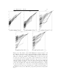
1
>>>
>>>
>>>
>>>
>>>
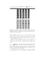
import ni
data = ni.data.monkey.Data(condition = 0)
model = ni.model.ip.Model({’cell’:4,’crosshistory’:[6,7]})
fm = model.fit(data.trial(range(data.nr_trials/2)))
plot(fm.prototypes()[’rate’],’k’)
>>> with ni.figure("",close=False):
plot(fm.prototypes()[’autohistory’],’k-’)
plot(fm.prototypes()[’crosshistory6’],’k--’)
plot(fm.prototypes()[’crosshistory7’],’k:’)
Bootstrapping Information Criterion for
Stochastic Models of Point Processes
&
The ni. Python Toolbox
Jacob Huth
University of Osnabrück
26 November 2013
Contents
Versicherung an Eides statt
1 Introduction
1.1 Comparing Models . .
1.1.1 The Problem of
1.1.2 The Problem of
1.1.3 Toolbox . . . .
3
.
.
.
.
.
.
.
.
.
.
.
.
.
.
.
.
.
.
.
.
.
.
.
.
.
.
.
.
.
.
.
.
.
.
.
.
.
.
.
.
.
.
.
.
.
.
.
.
5
5
6
6
7
. . . . . . .
. . . . . . .
. . . . . . .
. . . . . . .
. . . . . . .
. . . . . . .
. . . . . . .
. . . . . . .
. . . . . . .
. . . . . . .
the Model
.
.
.
.
.
.
.
.
.
.
.
.
.
.
.
.
.
.
.
.
.
.
.
.
.
.
.
.
.
.
.
.
.
.
.
.
.
.
.
.
.
.
.
.
.
.
.
.
.
.
.
.
.
.
.
.
.
.
.
.
.
.
.
.
.
.
.
.
.
.
.
.
.
.
.
.
.
.
.
.
.
.
.
.
.
.
.
.
.
.
.
.
.
.
.
.
.
.
.
.
.
.
.
.
.
.
.
.
.
.
.
.
.
.
.
.
.
.
.
.
.
8
8
8
9
9
10
10
12
12
13
13
15
. . . . . . . .
Over-Fitting
Bias . . . . .
. . . . . . . .
2 The
2.1
2.2
2.3
2.4
2.5
GLM Pointprocess model
Definition of a Model . . . . . . .
. . . . . . . . . . . . . . . . . . .
Notations . . . . . . . . . . . . .
Generalized Linear Models . . . .
Properties of Spike Trains . . . .
2.5.1 The Sifting Property . . .
2.6 Splines . . . . . . . . . . . . . . .
2.7 Rate Model . . . . . . . . . . . .
2.8 First Order History . . . . . . . .
2.9 Higher Order History . . . . . . .
2.10 How the Components are Used in
3 Python for Scientific Computations
3.1 Python Modules . . . . . . . . . .
3.2 Naming Convention . . . . . . . .
3.3 Exceptions in Python . . . . . . .
3.4 Context Managers . . . . . . . . .
3.5 Documentation . . . . . . . . . . .
.
.
.
.
.
.
.
.
.
.
.
.
.
.
.
.
.
.
.
.
.
.
.
.
.
.
.
.
.
.
.
.
.
.
.
.
.
.
.
.
.
.
.
.
.
.
.
.
.
.
.
.
.
.
.
.
.
.
.
.
.
.
.
.
.
.
.
.
.
.
.
.
.
.
.
.
.
.
.
.
.
16
17
17
17
18
20
4 Modules of the ni. Toolbox
4.1 ni.config - Toolbox Configuration Options .
4.2 Providing Data: the ni.data Modules . . . .
4.2.1 ni.data.data - a Common Structure
4.2.2 ni.data.monkey . . . . . . . . . . . .
4.3 Providing Models: the ni.model Modules .
.
.
.
.
.
.
.
.
.
.
.
.
.
.
.
.
.
.
.
.
.
.
.
.
.
.
.
.
.
.
.
.
.
.
.
.
.
.
.
.
.
.
.
.
.
.
.
.
.
.
.
.
.
.
.
.
.
.
.
.
22
22
23
23
25
25
1
.
.
.
.
.
.
.
.
.
.
.
.
.
.
.
.
.
.
.
.
Contents
4.3.1
4.3.2
4.4
4.3.3
4.3.4
4.3.5
Tools
4.4.1
4.4.2
4.4.3
4.4.4
4.4.5
4.4.6
2
.ip - Inhomogeneous Pointprocess Standard Model . . . .
4.3.1.1 Generating a Design Matrix . . . . . . . . . . .
4.3.1.2 Model Backends . . . . . . . . . . . . . . . . . .
4.3.1.3 Results of the Fit . . . . . . . . . . . . . . . . .
.designmatrix - Data-independent Independent Variables
4.3.2.1 Constant and Custom Components . . . . . . .
4.3.2.2 Rate . . . . . . . . . . . . . . . . . . . . . . . . .
4.3.2.3 Adaptive Rate . . . . . . . . . . . . . . . . . . .
4.3.2.4 Autohistory and Crosshistory . . . . . . . . . . .
4.3.2.5 2nd Order History Kernels . . . . . . . . . . . .
.ip generator - Turning Models back into Spike Trains . .
.net sim - A Generative Model . . . . . . . . . . . . . . .
.pointprocess - Collection of Pointprocess Tools . . . . .
ni.tools . . . . . . . . . . . . . . . . . . . . . . . . . . . . .
.pickler - Reading and Writing Arbitrary Objects . . . . .
.bootstrap - Calculating EIC . . . . . . . . . . . . . . . .
.project - Project Management . . . . . . . . . . . . . . .
4.4.3.1 Parallelization . . . . . . . . . . . . . . . . . . .
.plot - Plot Functions . . . . . . . . . . . . . . . . . . . .
4.4.4.1 plotGaussed . . . . . . . . . . . . . . . . . . . .
4.4.4.2 plotHist . . . . . . . . . . . . . . . . . . . . . . .
4.4.4.3 plotNetwork and plotConnections . . . . . . . .
statcollector - Collecting Statistics . . . . . . . . . . . . .
html view - Collecting and Rendering HTML Output . .
4.4.6.1 Figures in View Objects . . . . . . . . . . . . . .
25
26
26
27
27
27
28
28
28
29
30
31
32
32
32
33
33
34
37
37
37
37
39
40
41
5 Bootstrapping an Information Criterion
42
5.0.7 AIC . . . . . . . . . . . . . . . . . . . . . . . . . . . . . . 42
5.0.8 BIC . . . . . . . . . . . . . . . . . . . . . . . . . . . . . . 43
5.0.9 EIC . . . . . . . . . . . . . . . . . . . . . . . . . . . . . . 44
5.0.9.1 Resampling by Creating More Spike Trains . . . 45
5.0.9.2 A Range of Criteria . . . . . . . . . . . . . . . . 45
5.1 Experiment 1 . . . . . . . . . . . . . . . . . . . . . . . . . . . . . 46
5.1.1 Results . . . . . . . . . . . . . . . . . . . . . . . . . . . . 48
5.1.1.1 Fitted Multi-Model . . . . . . . . . . . . . . . . 48
5.1.1.2 Information Criteria . . . . . . . . . . . . . . . . 50
5.1.1.3 A First Look at the Information Criteria . . . . 53
5.1.1.4 AIC . . . . . . . . . . . . . . . . . . . . . . . . . 53
5.1.1.5 BIC . . . . . . . . . . . . . . . . . . . . . . . . . 54
5.1.1.6 EIC . . . . . . . . . . . . . . . . . . . . . . . . . 55
5.1.1.7 variance reduced EIC using time reshuffle (𝑣𝑟𝐸𝐼𝐶)
- Trial Reshuffling vs. Time Reshuffling . . . . . 55
5.1.1.8 variance reduced EIC using a simple model (𝑣𝑟𝐸𝐼𝐶𝑠𝑖𝑚𝑝𝑙𝑒 )
- The Simple Model . . . . . . . . . . . . . . . . 57
5.1.1.9 variance reduced EIC using a complex model
(𝑣𝑟𝐸𝐼𝐶𝑐𝑜𝑚𝑝𝑙𝑒𝑥 ) - The Complex Model . . . . . . 57
Contents
5.2
5.1.1.10 The EIC Bias . . . . . . . . . . . . . . . . . . .
5.1.1.11 Information Gain and Network Inferences . . . .
5.1.2 Discussion . . . . . . . . . . . . . . . . . . . . . . . . . . .
Experiment 2 - Using Information Criteria for Parameter Selection
5.2.1 Results . . . . . . . . . . . . . . . . . . . . . . . . . . . .
5.2.2 Discussion . . . . . . . . . . . . . . . . . . . . . . . . . . .
3
57
58
63
63
63
65
6 Conclusions
68
6.1 The Differences between AIC, BIC and EIC . . . . . . . . . . . . 68
6.2 The Difference between Conservative and Variance Reduced EIC 69
6.2.1 The Difference between Trial Based and Time Based Resampling for EIC . . . . . . . . . . . . . . . . . . . . . . . 69
6.2.2 The Differences between EIC with Simple and Complex
Models . . . . . . . . . . . . . . . . . . . . . . . . . . . . 70
6.2.3 Summary conservative EIC using time reshuffle (𝐸𝐼𝐶) . . 70
6.3 Further Applications of the Toolbox . . . . . . . . . . . . . . . . 71
Bibliography
71
List of Figures & Acronyms
73
6.4 Acronyms . . . . . . . . . . . . . . . . . . . . . . . . . . . . . . . 75
Appendices
76
A Using the Toolbox
77
A.1 Setting up a the Necessary Python Packages on Your Own Computer . . . . . . . . . . . . . . . . . . . . . . . . . . . . . . . . . . 77
A.2 Using the iPython Notebooks or Qtconsole . . . . . . . . . . . . 78
A.3 Setting up a Private Python Environment . . . . . . . . . . . . . 78
A.4 Setting up the Toolbox . . . . . . . . . . . . . . . . . . . . . . . . 79
A.5 ssh and Remote Access to the Institut für Kognitionswissenschaft
Osnabrück (IKW) Network . . . . . . . . . . . . . . . . . . . . . 79
A.5.1 Setting up Public Key Authentification . . . . . . . . . . 79
A.6 Creating a Project . . . . . . . . . . . . . . . . . . . . . . . . . . 80
A.6.1 Inspection of Progress . . . . . . . . . . . . . . . . . . . . 81
A.7 Extending the Toolbox . . . . . . . . . . . . . . . . . . . . . . . . 81
Versicherung an Eides statt
Hiermit erkläre ich diese Masterarbeit selbständig verfasst und nur die angegebenen Quellen und Hilfsmittel verwendet zu haben.
4
Chapter 1
Introduction
This thesis presents a toolbox for modeling neuronal activity in the framework of
statistical models. A process of model selection is discussed, using the Extended
Information Criterion (EIC) to obtain a way of comparing models of varying
complexity.
Chapter 2 will introduce a model that can be used to predict neural activity using a Generalized Linear Model (GLM) and separate components to
model rate, autohistory and interactions with other cells. Chapter 3 refreshes
some concepts used in the Python programming language, such that chapter 4
can introduce the ni. toolbox and how it implements the model of chapter 2
(Section 4.3.1), represents data (Section 4.2) and provides tools for the utilization of the IKW computing grid and result presentation (Section 4.4). Chapter
5 then illustrates how to perform model selection using the toolbox and how
the bootstrapped information criterion compares to less computationaly intense
measures such as Akaike Information Criterion (AIC) and Bayesian Information
Criterion (BIC) (introduced in 5.0.7 and 5.0.8).
1.1
Comparing Models
For neuronal activity, prediction is no goal in itself, as it is eg. for weather
models. Rather, how good a model matches the actual activity gives insight
into the process behind the activity. When two models are compared, the one
that matches the data more closely can be considered as more representative
for the physical process. The structural differences between the models, such
as an interaction between two certain cell assemblies,can then be interpreted as
structural features of the physical process. But when data is finite, the problem
of over-fitting and the problem of biased estimators arise.
5
1.1.1 Comparing Models - The Problem of Over-Fitting
1.1.1
6
The Problem of Over-Fitting
When only a finite amount of data is used to fit a model, the model has to
extract characteristics from the data and interpolate how further data samples
might look like. A model that is more complex than the process behind the data
tends to infer behavior in the data that in actuality is never found because, as
the model is fitted, it will adapt to noise in the data more effectively than a
simple model. A term that was supposed to model an interaction between two
cells now models the interaction of one of those cells and a very specific instance
of noise fluctuations. By modeling the noise, the complex model can achieve a
closer fit to the training data, but it will have problems predicting new data, as
the noise is not a part of the modeled process and therefore not present in the
new data.
Such a model is said to have over-fitted. It tried to match the training data
as accurately as possible, and in doing so it missed the essential characteristics
of the process that it could have found in other instances of data.
1.1.2
The Problem of Bias
When a model is evaluated in how close it can predict data it was trained on,
an over-fitting model will (by defintion) always score better than a simpler, but
more representative model. The likelihood is biased - it will systematically be
estimated higher than it actually is on unseen data. So not only is a complex
model bad at predicting future data, it also overestimates its ability to do so.
But evaluating a model by comparing it to newly acquired data is difficult.
Take eg. the case of electrode recordings: the relative position to cell assemblies
and changes by neural plasticity or the physical insertion of the electrodes can
change the recorded activity in such a way that the previous model no longer
applies to new recordings that are taken some weeks after the first. Thus, a split
of the data of one recording session into a part that is used for training and a
part that is used for fitting is the most common method to evaluate models
and perform a model selection. Some models use model selection in their own
fitting process. This requires additional splits of the data into quarters, eights,
sixteenths, etc.
It would be much more practical if one could use the data one has to acquire
anyway to fit the model to also evaluate the model. To accomplish this, the bias
of the likelihood has to be estimated and compensated for to obtain an unbiased
information criterion, which judges how well a model explains the data.
As the bias tends to scale with complexity, one method to do this is to
subtract a penalty for each used parameter in the model. The AIC (see Section
5.0.7) builds on this principle. However, the bias is different on different data
statistics, which is why [Ishiguro et al., 1997] proposed a bias correction that
uses the bootstrapping method to simulate data fluctuations. This method is
discussed in section 5.0.9 and in chapter 5 the ni python toolbox will be used to
build a number of models, to compare them and to infer connectivity hypotheses
solely on the basis of evaluations using training data, which are then compared
1.1.3 Comparing Models - Toolbox
7
to evaluations using previously unseen data.
1.1.3
Toolbox
The toolbox can be obtained from: https://github.com/jahuth/ni/
The documentation is available at: http://jahuth.github.io/ni/
index.html and additional information on how to use the toolbox is in the
appendix of this thesis.
Chapter 2
The GLM Pointprocess
model
2.1
Definition of a Model
A model is a mapping from parameters into a probability distribution on features. The direction from parameters to features is called a prediction, the
inverse mapping, from features to parameters, is called the fit.
How good a model matches a physical process can be measured by comparing
the prediction with the actual data, yielding a likelihood of the data, given the
model.
One goal of modeling would be to infer facts about the world from the
parameters of the model that describes the data best. If a parameter in a model
makes it believable that some interaction between two neurons is taking place,
one would like to think that this interaction is actually plausible.
To find out whether the parameters actually represent hidden qualities of
the data, one can evaluate the model by cross evaluation, ie. fitting on some
part of the data and predicting the remaining part.
2.2
The goal of the models discussed in this thesis is to predict the firing probability
of a cell assembly at some time 𝑡 dependent on the previous time steps of the
same and other assemblies, using model components that each model a part of
the probability:
𝑝(𝑥(𝑡) = 1|𝑥(𝑡𝑡−1 ), . . . 𝑥(𝑡0 )) =
∑︁
· 𝑝𝑖 (𝑥(𝑡) = 1|𝑥(𝑡 − 1), . . . 𝑥(1), 𝑥(0)) (2.1)
𝑖
8
2.3 Notations
2.3
9
Notations
To make indexing parts of a spike train easier, we use a notation that selects a
range of values between two indices, including the first, but excluding the last
index:
⎧
⎪
⎨𝑥(𝑎), 𝑥(𝑎 + 1), . . . 𝑥(𝑏 − 1) if 𝑎 > 𝑏
𝑥[𝑎:𝑏] := 𝑥(𝑎), 𝑥(𝑎 − 1), . . . 𝑥(𝑏 + 1) 𝑖𝑓 𝑏 > 𝑎
(2.2)
⎪
⎩
𝑥(𝑎)
𝑒𝑙𝑠𝑒
The vector 𝑥[𝑎:𝑏] is therefore |𝑏 − 𝑎| elements long.
The set of spikes up to a timepoint 𝑡 will be denoted as:
𝑆𝑡 := {𝜏 |𝑥(𝜏 ) = 1 and 𝜏 < 𝑡}
(2.3)
With this notation Equation 2.1 becomes:
𝑝(𝑥(𝑡) = 1|𝑥[𝑡:0] ) = Π · 𝑝𝑖 (𝑥(𝑡) = 1|𝑥[𝑡:0] )
𝑖
2.4
(2.4)
Generalized Linear Models
To now model the probability with a Generalized Linear Model (GLM), we
rewrite 2.4 using some functions 𝑓𝑖 and a link function 𝑔 as:
(︃
)︃
∑︁
−1
𝑝(𝑥(𝑡) = 1|𝑥[𝑡:0] ) = 𝑔
𝛽𝑖 · 𝑓𝑖 (𝑥[𝑡:0] )
(2.5)
𝑖
𝑔 is a link function, 𝑓𝑖 are arbitrary functions and 𝛽𝑖 are coefficients. The linear
combination of the weighted functions, scaled by the link function, is used to model the
probability of a spike for each time point 𝑡.
The 𝛽𝑖 coefficients are what is to be optimized in the fitting process of
the GLM. The index 𝑖 runs over a set of functions that can be grouped into
Components that each model a certain aspect of the spike train.
To predict a Bernoulli distribution, 𝑔 should be the logit function, which is
the inverse of the logistic function (see Figure 2.4.1 and Equation 2.7). The
logistic function maps the real line into an interval between 0 and 1, such that
probabilities can be represented as arbitrarily large values. The larger a value
is, the closer the probability is to 1. The more negative it is, the closer the
probability is to 0. A value of 0 translates to a 0.5 probability.
𝑙𝑜𝑔𝑖𝑡(𝑝) = 𝑙𝑜𝑔(𝑝) − 𝑙𝑜𝑔(1 − 𝑝)
𝑙𝑜𝑔𝑖𝑡−1 (𝑥) =
1
1 + 𝑒−𝑥
(2.6)
(2.7)
2.5 Properties of Spike Trains
10
Figure 2.4.1: The logistic function, which is used to map values into probabilities. The logit function (the inverse of the logistic function) is used to map
probabilities to values.
2.5
Properties of Spike Trains
Spike trains can be written as a sum of Dirac 𝛿 functions:
𝑛
∑︁
𝜌(𝑡) =
𝛿(𝑡 − 𝑡𝑖 )
𝑖=1
𝑡𝑖 is spike number 𝑖, 𝑛 being the number of spikes. See also [Dayan and Abbott, 2001]
The Dirac 𝛿 function is defined on a discrete timeline1 at time 𝑡 as:
{︃
1 for 𝑡 = 0
𝛿(𝑡) =
0 𝑒𝑙𝑠𝑒
The function 𝜌(𝑡) will be zero almost everywhere, except at the time points
that contain a spike. An integral over a portion of this function will yield the
number of spikes in this portion.
2.5.1
The Sifting Property
A Dirac 𝛿 function has the property of selecting a value from a function when
applied in an integral or sum:
∫︁
𝑑𝜏 𝛿(𝑡 − 𝜏 )ℎ(𝜏 ) = ℎ(𝑡)
Which means, that if a kernel is multiplied with a spike train, the kernel can
be thought of as being filtered at each spike for its value. If a kernel is folded
1 On
the real numbers the definition differs, but this does not need to concern us as we only
use discrete time.
2.5.1 Properties of Spike Trains - The Sifting Property
11
on a spike train, the reverse kernel is appended to each spike. A kernel that is
defined on negative values (“looking into the past”) will project the influence of
the spike forward in time.
This means that if we want to calculate the influence on some time 𝑡 by
some spikes and a kernel, it is equivalent to express the influence as Equation
2.8 as a sum over time-points or 2.9 as a sum over the set of spikes. Since there
are less spikes than time points, the second method results in less computation.
∑︁
𝑓 (𝑡) =
𝑥(𝑡 − 𝜏 ) · 𝑘𝑒𝑟𝑛𝑒𝑙(𝜏 )
(2.8)
𝜏
𝑓 (𝑡) =
∑︁
𝑘𝑒𝑟𝑛𝑒𝑙(𝑠 − 𝑡)
(2.9)
𝑠∈𝑆
The following code illustrates the two formulas:
import scipy
spikes = np.zeros(1000)
for i in rand(10) * 1000:
spikes[int(i)] = 1
kernel = np.zeros(100)
kernel[70] = 1
kernel = scipy.ndimage.gaussian_filter(kernel,10)
# first method:
out = np.zeros(1100)
for t in range(1100):
out[t] = 0
for tau in range(100):
if (t-tau) >= 0 and (t-tau) < 1000:
out[t] = out[t] + (spikes[t-tau] * kernel[tau])
# second method
out2 = np.zeros(1100)
for t in where(spikes)[0]:
out2[t:(t+100)] = out2[t:(t+100)] + kernel
Figure 2.5.1: Using the sifting property, spike influence can be calculated in
O(spikes), rather than O(timesteps): The first method computes the sum of the
kerneled spikes for every time point (looking back), the second method adds up
time shifted kernels (looking forward in time). Both methods are equivalent.
2.6 Splines
2.6
12
Splines
To utilize the linear combination of functions in the GLM to model smooth
time series, these time series are approximated as splines, made up of a linear
combination of basis splines (b-splines). They are written as a small, bold b in
this text, with a lower index signifying that a certain basis spline out of a set is
considered. The number of basis splines in a set is referred to as 𝑘.
The basis splines in the FMTP [Costa, 2013] code and hence the ni. toolbox
are created recursively with the formulas (originally implemented by Niklas
Wilming for the NBP eye-tracking toolbox):
{︃
1 if 𝑥 lies between the knots 𝑗 and 𝑗 + 1
𝐵𝑗,1 (𝑥) :=
(2.10)
0 𝑒𝑙𝑠𝑒
and to calculate b-splines of an order 𝑘:
𝐵𝑖,𝑘 (𝑥) :=
𝑡𝑖+𝑘 − 𝑥
𝑥 − 𝑡𝑖
· 𝐵𝑖,𝑘−1 (𝑥) +
· 𝐵𝑖+𝑘,𝑘−1 (𝑥)
𝑡𝑖+𝑘 − 𝑡𝑖
𝑡𝑖+𝑘 − 𝑡𝑖+1
(2.11)
To compute basis spline 𝑖 of order 𝑘 at point 𝑥, the recursive formula computes a
weighted average between the lower order splines of this and the 𝑘-next index, weighted
by the relative distance to each of the knots.
2.7
Rate Model
To model rate fluctuations that are similar across all trials (or a subset, ie. all
trials with a certain condition), a spline function is spanned over the entire trial
duration, being separated in 𝑘 basis splines.
𝑓𝑟𝑎𝑡𝑒 (𝑡) = 𝑏0 +
𝑘
∑︁
𝛽𝑖 b𝑖 (𝑡)
(2.12)
𝑖=1
Figure 2.7.1: A set of rate basis splines and an example of a fitted spline.
2.8 First Order History
2.8
13
First Order History
Since spikes are also dependent on the activity of other regions and its own
history, it makes sense to model this term relative to the current time bin. We
should assume, that events in the very distant past are negligible in relation to
recent events and model only a time interval between 𝑡 and 𝑡 − 𝑚, with 𝑚 being
the length of memory that is assumed. If one argues that the further a spike
is in the past, the less important its exact location becomes, one should use
a logarithmic spaced spline function to model this, if one disagrees, a regular
spline spacing is also possible.
𝑓ℎ𝑖𝑠𝑡𝑜𝑟𝑦 (𝑥[𝑡:0] ) = 𝑏0 +
𝑘
∑︁
𝛽𝑖 b𝑇𝑖 𝑥[𝑡:𝑡−𝑚]
(2.13)
𝑖=1
This history term can be used without modification on other spike trains,
such that it models 𝑝(𝑥𝑎 = 1|𝑥𝑏[𝑡:0] )
(a)
(b)
(c)
Figure 2.8.1: (a) a set of history basis splines, (b) the components folded on a
spike train and (c) an example of a fitted spline.
2.9
Higher Order History
The first order history term has the fault that a fine grained placement of spikes
(eg. in bursting activity) is averaged into a single history term. To differentiate
behavior in high firing rate regimes and low firing rate regimes, one needs to
include more than one spike at a time in the model.
Taking spikes at two distances 𝑖 and 𝑗 in the spike train past, we would want
to model interactions that influence the current bin as:
𝑓2𝑛𝑑
ℎ𝑖𝑠𝑡𝑜𝑟𝑦 (𝑥[0:𝑡] )
=
𝑚 ∑︁
𝑚
∑︁
ℎ(𝑖, 𝑗)𝑥(𝑡 − 𝑗)𝑥(𝑡 − 𝑖)
(2.14)
𝑖=1 𝑗=1
ℎ(𝑖, 𝑗) models the interactions of spikes at time 𝑡 − 𝑖 and 𝑡 − 𝑗. The term 𝑥(𝑡 − 𝑗)𝑥(𝑡 − 𝑖)
selects an value out of the ℎ matrix at entry 𝑖, 𝑗.
2.9 Higher Order History
14
If we assume ℎ(𝑖, 𝑗) not to be arbitrary and sparse, but rather a smooth surface,
we have to use splines again to fit this surface to the few data points we have:
ℎ(𝑖, 𝑗) =
𝑘1 ∑︁
𝑘2
∑︁
𝛽𝑖1 ,𝑖2 b𝑖1 (𝑖)b𝑖2 (𝑗)
(2.15)
𝑖1 =1𝑖2 =1
𝑚 being the memory length of the history component, 𝑘1 being the number of splines
in the first set, 𝑘2 the number in the second.
Following [Schumacher et al., 2012], the coefficients can be taken out of the
multiplication of spike trains, such that the spike trains folded with each basis
spline can be multiplied with each of the other folded spike trains to get each
component across the complete trial interval.
𝑓2𝑛𝑑
ℎ𝑖𝑠𝑡𝑜𝑟𝑦 (𝑥[0:𝑡] )
=
𝑘1 ∑︁
𝑘2
∑︁
𝛽𝑖1 ,𝑖2
𝑖1 =1𝑖2 =1
(︃ 𝑚
∑︁
⎞
)︃ ⎛ 𝑚
∑︁
b𝑖1 (𝑖) · 𝑥(𝑡 − 𝑖) · ⎝ b𝑖2 (𝑗) · 𝑥(𝑡 − 𝑗)⎠
𝑖=1
𝑗=1
(2.16)
Because of symmetry the term in the sum of 𝑗 in Equation 2.15 can be
restricted to 𝑗 > 𝑖, if we use the same(︃basis functions for)︃every dimension.
𝑚
∑︀
Then, however, we can no longer isolate
b𝑖2 (𝑗) · 𝑥(𝑡 − 𝑗) as a single term,
𝑗>𝑖
since it would then depend on 𝑖.
But using the symmetry for the case of using the same basis splines, the
number of coefficients can be reduced, as the coefficient 𝛽𝑎,𝑏 will have the same
independent variables as 𝛽𝑏,𝑎 , since the same spikes are concerned. This would
result in 𝛽𝑎,𝑏 and 𝛽𝑏,𝑎 adding up to the actual interaction coefficient 𝛽𝑎,𝑏+𝑏,𝑎 .
So 𝛽𝑏,𝑎 can be set to 0 for all 𝑏 > 𝑎 to reduce the (apparent) model complexity:
𝑓2𝑛𝑑
ℎ𝑖𝑠𝑡𝑜𝑟𝑦 (𝑥[𝑡:0] )
=
𝑘1 ∑︁
𝑘2
∑︁
𝑖1 =1𝑖2 ≥𝑖1
⎞
)︃ ⎛ 𝑚
(︃ 𝑚
∑︁
∑︁
𝛽𝑖1 ,𝑖2
b𝑖1 (𝑖) · 𝑥(𝑡 − 𝑖) ·⎝ b𝑖2 (𝑗) · 𝑥(𝑡 − 𝑗)⎠
𝑖=1
𝑗=1
(2.17)
𝑚 being the memory length of the history component, 𝑘1 being the number of splines
in the first set b𝑖1 , 𝑘2 the number in the second set b𝑖2 . The coefficients 𝛽𝑖1 ,𝑖2 will be
re-indexed in the model.
The model component implementing this part of the model will be discussed in
Section 4.3.2.5.
2.10 How the Components are Used in the Model
2.10
15
How the Components are Used in the Model
The standard model provided by the ni. toolbox is a combination of a rate
model, an autohistory model and a crosshistory model for each cell in the data.
Additional parts can be added to the model by editing the Configuration of the
model (eg. a higher order autohistory term). To fit the model, or to predict
data, a design matrix is constructed using these Components (see Section 4.3.2)
and spike data, calculating 𝑓𝑐𝑖 (𝑡) for 𝑡 ∈ [0 . . . 𝑇 ] and all parts of all components
𝑐𝑖 .
The resulting matrix is then used to calculate the optimal coefficients 𝛽𝑖 to
maximize the likelihood of Equation 2.5 using one of the statistical modeling
python libraries (see Section 4.3.1.2).
Since the model uses the linear combination of the single model components
𝑓𝑐𝑖 , the formulas of this section are always used as a given, fixed time series
- whether fitting or predicting. They are calculated once from a set of spikes,
creating a series of values. Afterwards the mathematical definition of each
component is no longer considered in the fitting or prediction process. The
only exception is when spikes are generated from an existent model (see Section
4.3.3) in the case of first order history components. To make computation easier,
rather than re-calculating the complete 𝑓𝑎𝑢𝑡𝑜ℎ𝑖𝑠𝑡𝑜𝑟𝑦 component whenever a spike
is set, the fitted spline function of the autohistory component is added to the
rate function, essentially adding up to the definition in Equation 2.13.
Chapter 3
Python for Scientific
Computations
Python is a programming language developed for code readability and (relative)
platform independence. It is an interpreted language as it is not translated into
architecture-dependent machine code, but run inside an interpreter. Computationally expensive operations can be handled by platform specifically compiled
libraries written in C or Assembler.
The scipy project1 , including the packages matplotlib, numpy, scikit (and
many more) and the interactive iPython console, enable python to be useful
for scientific computations, such as large scale data analysis and visualization,
statistical modeling and even symbolic mathematics2 .
Python uses indentation levels to indicate program flow. Variables are
loosely typed and can contain different types at different time points. Lists
and dictionaries are built-in types that can save an array of variables, indexed
with a number for lists or indexed by a string for dictionaries.
Python packages are organized in modules (see Section 3.1). Modules, classes
and functions are named as described in Section 3.2. Exceptions and Context
Managers are two concepts used in the toolbox that make code more readable
and act reasonable in case of errors. Sections 3.3 and 3.4 give a short introduction to these concepts. Source code is only useful when properly documented.
The sphinx package can create html documentation from python code as described in 3.5.
A local git repository has been used for private version control and to
publish code easily to the IKW servers. The release version is published on
github: https://github.com/jahuth/ni/ along with the documentation
at http://jahuth.github.io/ni/index.html
1 http://www.scipy.org/
2 http://www.sympygamma.com/input/?i=limit%28x
16
*log%28x%29%2C+x%2C+0%29
3.1 Python Modules
3.1
17
Python Modules
Python provides object oriented programming mechanisms that make it easy to
encapsulate code such that it does not interfere with other parts of the program.
Classes and functions can be part of a module (in the simplest case a .py file)
that can be included in programs and provides a save name space for these
classes and functions.
The ni. toolbox is a module that includes other modules for easy access.
They are grouped in three sub-modules ni.data., ni.model. and ni.tools. which
in turn contain the modules for data representation, modeling and miscellaneous
tasks respectively.
When a module is included in a script, it is compiled to python byte-code,
which means that the module only needs to be parsed once by the python parser
and - if no changes are made to the module - can be accessed almost as fast as
a binary library.
3.2
Naming Convention
Based loosely on [van Rossum et al., 2001], the following conventions were followed for naming:
∙ All lowercase for modules: module. Underscores may be used to improve
readability as in ni.tools.html view.
∙ Class names are CamelCase, starting with a capital letter and starting
each new word with a capital letter with no underscores, colons, etc. separating words.
∙ Functions and methods are named all lower case with underscores or
camelCaseStartingWithLowerLetter, arguments of functions and methods are named similarly. If a verb as a name for a function is modified in
the text of this thesis, only the actual name of the function is printed as
a keyword.
∙ A leading underscore is used to signify that an attribute is hidden
∙ module wide constants are all CAPITAL LETTERS, words separated by
underscores.
3.3
Exceptions in Python
Contrary to most languages, exceptions in python are expected to come up.
They even are preferred to return values such as False, 0 or -1 for unsuccessful
function calls (if eg. a file can not be opened). If an exception is not handled
by an except: block, it will be raised to the user, showing a backtrace of what
lead to the exception. Still, exceptions should only be handled for specific cases
3.4 Context Managers
18
and seldom with a catch-all, except for code that runs in a sandbox or contains
user written code.
An example for how exceptions are used as a language feature is the following:
x1 = randint(10)
x2 = randint(10)
y = randint(10)
if (x1-x2) != 0:
ratio = y/(x1-x2)
else:
ratio = y
x1 = randint(10)
x2 = randint(10)
y = randint(10)
try:
ratio = y/(x1-x2)
except ZeroDivisionError:
ratio = y
When code in a try: block fails, the except Handler: block is asked to handle
the exception. If no handler matches the exception, it is raised further. If one
were to signal a non-existent file or some inconsistent arguments in some innermost function code using return codes such as False, 0, -1, or even predefined
constants, every function that uses some code that could fail and fails with it,
would have its return value checked whether something went wrong. Exceptions
bypass all of this, straight to the code that actually knows what to do in case
of non-existent files or inconsistent arguments.
Using if-statements before calling a potentially failing function would not
always result in a manageable amount of checks and can interfere with encapsulation of object oriented programming, making it harder to exchange code that
has basically the same functionality, but eg. lacks some limitations (one example would be to go from a text-file based logging mechanism to a database).
With exceptions, deprecated limits do not need to be checked.
In the toolbox, exceptions are mostly raised as the default Exception type,
but using a custom messages like "End of Jobs".
3.4
Context Managers
A nice way that python uses to make writing code more easy are so called
Context Managers, which are objects that contain an enter and an exit
method (surrounded by two underscores). The most common example is the
built-in file type:
with open("a_master_thesis.txt", "w+") as f:
f.write("Some text.")
The function open returns a file object, which is also a Context Manager.
Instead of properly opening the file and closing it after writing to it is done, the
file is opened as soon as the context is entered. The indented code can access
the object under the name f and after the code is completed, the file is closed.
This is useful to improve the readability of ploting code. An example of
normal matplotlib plotting code would be:
3.4 Context Managers
19
fig = pylab.figure()
for (x,y) in data_1:
plot(x,y)
title("Important Data")
fig_2 = pylab.figure()
for (x,y) in data_2:
plot(x,y)
title("Other Data")
fig.savefig("plot_1.png")
fig_2.savefig("plot_2.png")
Similarly to matlab and R, the default matplotlib method is to save figure
handles in variables, while the active figure is remembered by the plotting library
and follows a stacking behavior: first-in, last-out. If one remembers the handle,
a previous figure can be activated at a later point, while the stack structure
remains intact.
The code can be rewritten to use Context Managers from the ni. toolbox:
with ni.View("results.html") as view:
with view.figure("plot_1.png"):
for (x,y) in data_1:
plot(x,y)
with view.figure("plot_1.png"):
for (x,y) in data_2:
plot(x,y)
title("Other Data")
title("Important Data")
Even if in this example no care was given to structure the code in terms of
which figure is plotted into at which time, the indentation makes it clear which
plot function call corresponds to which active figure. Since each figure is closed
at the exit call, the stack behavior is made explicit.3
This mechanism becomes useful particularly in the case of Exceptions (see
Section 3.3). If some code within the with block fails, the exit method will
still be called and also informed that an error took place so that files can be
closed and data can be cleaned up. Normally, figures would remain opened,
disturbing further code, clogging up memory and preventing partially finished
figures to be written to files. A Context Manager will close the figures and write
them to a file.
Classes in the toolbox that act as context managers are:
∙ ni.Figure, provided by the function ni.figure(filename), saves a figure as
if called via pylab.figure() and pylab.savefig(filename). Additionally, the
figure is closed unless ni.figure has been called with close=False, in which
case the previously active figure will be activated again.
∙ ni.tools.html view.Figure, provided by the .figure(path) method of the
View class saves a figure into the View object it was called from. The
figure will be transformed into a base 64 encoded string, such that it can
be included in an html file.
3 Of course there can be use cases where this behavior is detrimental to the flow of computation or memory usage. Figure handles can still be used.
3.5 Documentation
20
∙ The View class itself, if instantiated with a filename, renders the output
to the specified location.
3.5
Documentation
Python code should always be documented with doc-strings for every module,
class and function. Doc-strings are an integral part of the language and are
actually present whenever a function is used:
print ni.data.data.merge.__doc__
The iPython notebook and console provide the doc string as a tooltip and
the sphinx documentation package4 generates comprehensive html or pdf documentation from re-structured text (ReST) doc strings. The ni. toolbox documentation is available on http://jahuth.github.io/ni/index.html
Below, the first lines of the data module python file show an example of a
doc string that is compiled into the documentation (see Figure 3.5.1).
"""
.. module:: ni.data.data
:platform: Unix
:synopsis: Storing Point Process Data
.. moduleauthor:: Jacob Huth
.. todo::
Use different internal representations, depending on use. Ie. Spike times vs. binary array
.. todo::
Lazy loading and prevention from data duplicates where unnecessary. See also: ‘indexing view versus
copy <http://pandas.pydata.org/pandas-docs/stable/indexing.html#indexing-view-versus-copy>‘_
Storing Spike Data in Python with Pandas
-------------------------------------------------------The ‘pandas package <http://pandas.pydata.org/>‘_ allows for easy storage of large data objects in python.
The structure that is used by this toolbox is the pandas :py:class:‘pandas.MultiIndexedFrame‘ which is
a :py:class:‘pandas.DataFrame‘ / ‘pandas.DataFrame <http://pandas.pydata.org/pandas-docs/dev/dsintro.
html#dataframe>‘_ with an Index that has multiple levels.
The index contains at least the levels ‘‘’Cell’‘‘, ‘‘’Trial’‘‘ and ‘‘’Condition’‘‘. Additional Indizex can be
used (eg. ‘‘’Bootstrap Sample’‘‘ for Bootstrap Samples), but keep in mind that when fitting a model
only ‘‘’Cell’‘‘ and ‘‘’Trial’‘‘ should remain, all other dimensions will be collapsed as more sets of
Trials which may be indistinguishable after the fit.
===========
Condition
===========
0
0
0
0
0
...
1
1
...
===========
=====
Cell
=====
0
0
0
1
1
...
0
0
...
=====
=======
Trial
=======
0
1
2
0
1
...
0
1
...
=======
===================================
*t* (Timeseries of specific trial)
===================================
0,0,0,0,1,0,0,0,0,1,0...
0,0,0,1,0,0,0,0,1,0,0...
0,0,1,0,1,0,0,1,0,1,0...
0,0,0,1,0,0,0,0,0,0,0...
0,0,0,0,0,1,0,0,0,1,0...
...
0,0,1,0,0,0,0,0,0,0,1...
0,0,0,0,0,1,0,1,0,0,0...
...
===================================
To put your own data into a :py:class:‘pandas.DataFrame‘, so it can be used by the models in this toolbox
create a MultiIndex for example like this::
import ni
import pandas as pd
d = []
tuples = []
for con in range(nr_conditions):
"""
4 http://sphinx-doc.org/
3.5 Documentation
Figure 3.5.1: A sphinx documentation page
21
Chapter 4
Modules of the ni.
Toolbox
4.1
ni.config - Toolbox Configuration Options
Some variables have default values for the complete toolbox. To give the user
control over these variables, the ni.config saves and loads these variables from
the files: ni_default_config.json, ni_system_config.json and ni_
user_config.json. The default configuration file is part of the toolbox
and should not be altered, except when the changes are submitted back to the
toolbox repository. The system configuration file contains default changes that
can be made by administrators or course advisors and the user configuration
file should contain all preferences that only apply to the specific user.
For every option that is requested by the toolbox, first the user option is
used, if it exists. If it does not exist, the system option is used, if it is not set in
the system file either, the default value is used. However, code using the config
module should still have a default value ready, in case the default configuration
file is missing the specific option as well.
Configuration options can be changed directly in the files, if the json syntax
is maintained, or alternatively by calling ni.config.user.set(option, value)
and subsequently ni.config.user.save()
Using the options in the code is done by requesting an option with
ni.config.get(option, default_value).
To request all set options in all config files, ni.config.keys(True), lists them
in the order of over-ride. To get a list of only unique option names, the python
type set 1 can be used: set(ni.config.keys(True))
1 as
in set theory, not as a verb
22
4.2 Providing Data: the ni.data Modules
4.2
4.2.1
23
Providing Data: the ni.data Modules
ni.data.data - a Common Structure
Spike data can be organized via the Data class. It contains a Pandas MultiFrame, which contains rows of trials, indexed with Trial, Cell, Condition and
possible additional indices.
Pandas DataFrames are similar to DataFrames used in R (see eg. http://
stat.ethz.ch/R-manual/R-devel/library/base/html/data.frame.
html). DataFrames store data (eg. time series) of equal length. It is indexed
two-dimensionally and behaves very similar to two-dimensional matrices. But it
can also contain meta data to index entries in the DataFrame more elaborately.
For pandas specifically, a DataFrame can be thought of as an indexed collection
of Series, which are in some ways equivalent to numpy ndarrays.
A DataFrame can be build from a dictionary of Series, or from an unlabeled
matrix. To use a Hierarchical Index (MultiIndex), the index has to be created
such that it corresponds to the single entries in the DataFrame.
The following code demonstrates how to convert a 3d-indexed set of spike
time lists into a multi-indexed DataFrame:
from ni.model.pointprocess import getBinary
d = []
index_tuples = []
for condition in range(self.nr_conditions):
for trial in range(self.nr_trials):
for cell in range(self.nr_cells):
d.append(list(getBinary(spike_times[condition,trial,cell
].flatten()*resolution)))
index_tuples.append((condition,trial,cell))
index = pandas.MultiIndex.from_tuples(index_tuples, names=[’
Condition’,’Trial’,’Cell’])
data = pandas.DataFrame(d, index = index)
An example to use data from eg. the nltk toolkit would be to define points
on different channels as the occurrence of letters. This means eg. to have one
channel for word separators and one for one of the vowels a, e, i each and to take
different languages as conditions. To use this setup with the toolbox, models
simply convert the occurrences to binary arrays and add them to a list, with an
index tuple at the same position in the index list.
import ni
import numpy as np
import pandas
from nltk.corpus import genesis
from ni.model.pointprocess import getBinary
trial_length = 1000 # use blocks of this many characters as a trial
d = []
index_tuples = []
for (condition, txt_file) in enumerate([’english-kjv.txt’,’finnish.
txt’,’german.txt’,’french.txt’]):
s = genesis.raw(txt_file).replace(’.\n’,’ ’).replace(’\n’,’ ’).
replace(’.’,’ ’) # to make the end of sentences also ends of
words
4.2.1 Providing Data: the ni.data Modules - ni.data.data - a Common
Structure
24
for t in range(len(s)/trial_length):
for (cell, letter) in enumerate([’ ’, ’a’, ’e’, ’i’]):
d.append(list(getBinary( np.cumsum([len(w)+1 for w in s
[(t*trial_length):((t+1)*trial_length)].split(letter
)]) )))
index_tuples.append((condition,t,cell))
index = pandas.MultiIndex.from_tuples(index_tuples, names=[’
Condition’,’Trial’,’Cell’])
data = ni.Data(pandas.DataFrame(d, index = index))
model = ni.model.ip.Model({’history_length’:10, ’rate’:False})
for condition in range(4):
fm = model.fit(data.condition(condition).trial(range(50)))
print str(condition)+’: ’ + ’ ’.join([str(fm.compare(data.
condition(i).trial(range(50,100)))[’ll’]) for i in range(4)
])
Figure 4.2.1 shows spike plots for one trial. The likelihoods of the models trained
on each of the conditions will print as something like:
0:
1:
2:
3:
-363.370063515
-503.786012045
-392.585078922
-400.67833968
-547.122975071
-381.38280323
-492.461953592
-446.436570567
-381.937801005
-432.132176101
-354.180694395
-387.665897328
-454.057645381
-476.044628726
-453.905837921
-400.7340132
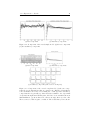
Figure 4.2.1: Using a few lines of code, data from other python toolkits like
the nltk can be used as pointprocess data. This plot shows one block of data
counting occurrences of word separators and the vowels a, e and i (as channels
0 to 3) in the (subplots from top to bottom) English, Finnish, German and
French version of the genesis corpus of the nltk.
Another example on how to create an actual data module can be found in
the appendix.
4.2.2 Providing Data: the ni.data Modules - ni.data.monkey
4.2.2
25
ni.data.monkey
For this module to work, the ni.data.monkey.path variable of the config
module has to be set to a directory containing the .mat files of the data from
[Gerhard et al., 2011] as provided to me by Gordon Pipa. This directory should
be accessible by the user and - if possible - from any machine in the IKW
network eg. on a network storage. While this module is mostly an example,
other spike data can be provided similarly in their own modules.
Using this data set (or any other that provides its own module) should be
as easy as:
import ni
ni.config.user.set("ni.data.monkey.path",
"/home/user/Data/Gerhard2011b")
data = ni.data.monkey.Data() # loads the first datafile
data.condition(0).cell([0,2,3]).trial(range(10)) # selects the first
ten trials of cells 0, 2 and 3 of condition 0
Or if the dataset offers additional parameters:
import ni
import random
trial_number = random.choice(ni.data.monkey.available_trials)
data = ni.data.monkey.Data(trial_number,condition=0,cell=[0,2,3],
trial=range(10))
# loads a specific data file and only loads the specified trials
, cells and condition
4.3
4.3.1
Providing Models: the ni.model Modules
.ip - Inhomogeneous Pointprocess Standard Model
A generalized linear model is a more flexible form of regression that uses a link
function to predict the value of a target function. In the case of spike trains, this
target function is 0 or 1, which means that 100% prediction is near to impossible
and the best one can do is to get the prediction function as low as possible when
there are no spikes and as high as plausible for when a spike is predicted.
If one takes the firing probability as a mean of a very large ensemble of
neurons, the prediction tries to accurately match the percentage of firing neurons
at any given time.
The model that is used for this toolbox contains methods to create a design
matrix, fit the model via the statsmodels.api.GLM [Perktold et al., 2013] class,
using the statsmodels.genmod.families.family.Binomial family to provide a
link function, or the sklearn.linear model.ElasticNet [scikit-learn developers, 2013]
To create a model, a Configuration instance or a dictionary containing configuration values is needed. Otherwise the default values are used.
Some important values are:
4.3.1 Providing Models: the ni.model Modules - .ip - Inhomogeneous
Pointprocess Standard Model
value
cell (int)
autohistory (bool)
crosshistory (bool or list)
rate (bool )
knots rate (int)
knots number (int)
history length (int)
backend "glm" or "elasticnet"
default
0
True
True
True
10
3
100
"glm"
26
description
The number of the dependent cell
Whether to include an autohistory component
Whether to include crosshistory components
Whether to include a rate component
Number of knots in the rate components
Number of knots in the history components
Length of the history components
Which backend to use
Table 4.1: Configuration values of the ip Model. A full description can be seen
in the documentation.
4.3.1.1
Generating a Design Matrix
Once the model is created, it can be used to .fit to data and .save itself to a
text file. Also it can .compare a predicted time series to point process data
using the appropriate functions.
In the Model.fit method, the dependent time series is extracted from the
data and a design matrix is created from the configuration values and the data
that is to be fitted to. The design matrix can also be obtained by the Model.dm
method, the dependent time series by the Model.x method.
The design matrix is created by creating a DesignMatrixTemplate (see Section 4.3.2) and adding a number of components to it (a HistoryComponent
on the dependent cell if autohistory is True, etc.). After all components are
added, the Template is combined with the data into an actual matrix, folding
the history kernels onto spikes, adding the rate splines once every trial etc..
The finished design matrix is then inspected for rows that are only 0. The
coefficients for these rows are set to zero.
4.3.1.2
Model Backends
When the .fit method of the selected backend is called, it chooses the coefficients,
such that the the likelihood of 𝑔 −1 (𝑌 · 𝛽) on the time series 𝑥 is maximal 2 . For
the "glm" backend this is done by the GLM function with an Binomial Family
object:
binomial_family = statsmodels.api.families.Binomial()
statsmodels.api.GLM(endog, exog, family=binomial_family)
with endog being the time series to predict and exog being the design matrix.
The "elasticnet" backend uses either the sklearn.linear model.ElasticNetCV()
to choose the regularization parameters by cross evaluation when the confguration option crossvalidation is set to True. Alternatively it uses the class
sklearn.linear model.ElasticNet() that uses an alpha and an l1_ratio value set
in the configuration.
2 𝑌 is the design matrix/independent variables, 𝛽 the coefficients and 𝑥 the independent
time series
4.3.2 Providing Models: the ni.model Modules - .designmatrix Data-independent Independent Variables
4.3.1.3
27
Results of the Fit
After the fit is complete, the results are saved in a FittedModel. This object
contains a reference to the model, the fitted coefficients as .beta and a range
of statistic values, as provided by the chosen backend. A FittedModel can be
.saved to a file, .predict other data and .compare the prediction to the actual
data using the methods provided by the model class. Also it can return a
dictionary of the fitted components added up to one prototype each.
4.3.2
.designmatrix - Data-independent Independent Variables
The ni.model.designmatrix module provides a class DesignMatrixTemplate
that stores design matrix Components. These components create rows for the
actual design matrix when provided with data. As some components may require nontrivial computation on the data (eg. higher order spike dependencies)
and the design matrix has to be computed completely from scratch for every
prediction, rather than the actual design matrix only the components are saved
in the model.
Rather than the actual design matrix, the model only remembers the template that was used to create the matrix. Since the design matrix is used at
most twice, but can become very large as it has dimensions of the trial duration
× the number of trials × the number of independent variables (ie. rows), a
huge amount of memory is used up unnecessarily, if a large number of models
is fitted for eg. bootstrapping or simple model comparison. Also the template
is necessary to create new design matrices for predicting other data.
4.3.2.1
Constant and Custom Components
Components that are added to the design matrix should be derived from the
class designmatrix.Component to make sure they contain all necessary methods
to function as a design matrix component. Also the bare Component class can
be used to insert arbitrary values into the design matrix.
The most trivial of all components is a constant that has to be added to
all models and just provides a means of shifting all other components by arbitrary amounts. It is sufficient to only add a single 1 as a kernel (using
numpy.zeros((1,1)) to make sure it is a two dimensional 1), as the kernel will
be repeated until the end of the time series.
When adding other time series as a kernel it should be noted that the correct orientation is used when adding the kernel to the component. The first
dimension should align with the time bins (eg. be equal to the trial length),
the second dimension holds different parts of the component, eg. different basis
splines.
To have one component trying to cover firing rate trends over multiple trials
one could write:
import ni
4.3.2 Providing Models: the ni.model Modules - .designmatrix Data-independent Independent Variables
28
data = ni.data.monkey.Data(condition=0)
long_kernel = ni.model.create_splines.create_splines_linspace(data.
nr_trials * data.trial_length,5,False)
ni.model.ip.Model({’custom_components’: [ ni.model.designmatrix.
Component(header=’trend’, kernel=long_kernel) ]})
4.3.2.2
Rate
A Rate component tries to model regular fluctuations of the firing rate that
is the same in all trials.3 This could be eg. the response to an experimental
stimulus. It is important to keep in mind that if this stimulus is not at exactly
the same point in time for all trials, one must rather encode the stimulus as an
additional spike train and use a crosshistory component to fit the response.
The normal rate component is the sum of a number of linearly spaced splines
that cover the whole trial duration. Each spline corresponds to a section of trial
time and will be scaled to the mean firing rate at that point (taking into account
other components as well). The sum of those splines gives a smooth function,
no matter how the individual splines are scaled.
RateComponents can be configured with the knots_rate option. The length
of the component is fixed to the trial length, but if a custom kernel is supplied,
the length is not checked. The DesignMatrix will revert to the default behavior
and concatenated the kernel on itself to fill the timeseries.
4.3.2.3
Adaptive Rate
If one suspects that some points in time require a higher resolution of modeling
- which is usually the case if there is a fluctuation of firing rate - one can use
a custom spacing of spline knots. The AdaptiveRate component will accept
custom spacings, but - if non is provided - will also compute a spacing that
will cover roughly the same number of spikes in each spline. Regions with
higher firing rate will have a higher resolution, thus the model is more sensitive
to firing rate changes, if the firing rate is high. Information theoretically this
makes sense, as a low firing rate is harder to predict than a higher firing rate
(as in a Poisson process, the variance scales with the firing rate), thus it should
be smoothed more to prevent over fitting. A high firing rate allows very fine
variations to be caught, which justifies a high resolution.
4.3.2.4
Autohistory and Crosshistory
To model how a neuron assembly regulates its own firing rate, eg. by a refractory period or self inhibition, one can use Equation 2.13 from Section 2.8 in a
HistoryComponent that is set to the same spike train that it predicts.
A HistoryComponent requires as arguments the cell it is based on as a
number (the channel), a length of memory (history_length), the number of
knots to span a logarithmic spline function (knot_number) and a boolean value
3 see
Section 2.7 for the mathematical definition
4.3.2 Providing Models: the ni.model Modules - .designmatrix Data-independent Independent Variables
(a)
29
(b)
(c)
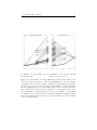
Figure 4.3.1: To model a rate function that has varying degrees of firing rate
such as (a), it might make sense to use a higher resolution on the sections of
the spike train that have a higher firing rate. (b) shows a comparison between
linear knot spacing and adaptive knot spacing, taking into account the firing
rate. (c) shows the resulting fitted rate functions: the grey lin-spaced rate
function can’t imitate the finer structures of the target. The black adaptive
rate spaced function does a better job with the same number of basis splines.
Tweaking the number of knots and the smooth-ness of the rate function used
for the component, a close fit is possible.
whether the last basis spline should be omitted. Alternatively, one can supply the HistoryComponent with a ready made kernel as produced by the create splines logspace or create splines linspace helper functions in the ni.model.
create splines module.
The default values for the automatically created auto- and crosshistory components is taken from the model configuration. Also the flags for which history
is to be considered are included in the configuration. The autohistory option
can either be True or False, while the crosshistory option can contain a list of
cell numbers that are to be used for history components.
4.3.2.5
2nd Order History Kernels
Higher order kernels, made up out of products of splines can be seen as the sum
of products of one dimensional basis splines as discussed in Section 2.9
The prototype of this component are not two fitted spline functions, but a
𝑘 × 𝑘 matrix relating spikes at time 𝑖1 and 𝑖2 to a specific firing rate probability. However the matrix is not symmetric, as presumed by the definition, but
4.3.3 Providing Models: the ni.model Modules - .ip generator - Turning
Models back into Spike Trains
30
(a)
(b)
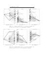
Figure 4.3.2: An example of a higher order history. (a) all combinations of
basis splines (b) the fitted component only uses the upper half of the diagonal
(including the diagonal combinations). Note that each matrix has some nonnegative values below its diagonal.
assumes an arbitrary order (𝑖1 < 𝑖2 or 𝑖2 < 𝑖1 pose no difference here). The
b-spline combinations for the lower diagonal were omitted, as they are equal to
the upper half. There are still some values below the diagonal non-zero, but this
is caused by the b-splines not ending at the diagonal. Hence the actual value is
not ℎ𝑖1 ,𝑖2 , but rather ℎ𝑖1 ,𝑖2 + ℎ𝑖2 ,𝑖1 .
This may seem as if the symmetry is unused, but as the symmetry was
actually used to reduce the number of coefficients, and the complexity trick of
Section 2.9 only works for non-ordered spikes, this was the most plausible course
of action.
4.3.3
.ip generator - Turning Models back into Spike Trains
To generate new spikes from a model, one can use the fitted components to
estimate a firing probability. This probability has to be scaled via the link
function to get an actual probability, which can then be instantiated by a coin
toss of exactly that probability for each bin.
In the simple rate-model case, this will generate a spike train that mimics
the mean firing rates for every bin. If autohistory or crosshistory models are
4.3.4 Providing Models: the ni.model Modules - .net sim - A Generative
Model
31
used to generate spikes, the corresponding firing rate deviations are dependent
on whether there was a spike in the past, ie. it depends on the coin tosses of
the previous bins. This means, that on every coin toss, that created a spike,
the history kernel has to be projected into future bins to modify the firing rate
probability.
For higher dimensional history kernels, the probability is determined by the
actual component on the basis of the previous spikes and kept separate from
the firing rate that is modified by the first order history.
The current implementation only works with the standard design components, ie. a RateComponent, a Component named ’constant’, optionally
auto- and cross HistoryComponents and higher order autohistory. If custom
components are added, the generator needs to be extended to include these components, otherwise the generated spikes will deviate from the model severely.
Figure 4.3.3: An example of created and predicted firing rates to test whether
the ip generator is functioning correctly.
A demo project illustrates, whether an implementation of a generator is
correct. It fits models on some random data and then generates a new trial.
Then the models are used to predict firing rate of the new trial. Since the
generator not only returns the spike times, but also the firing probability that
was used to generate the spikes, the firing rate probability can be compared.
Since the probability for the generator and the model only depends on the past,
the actual spikes that are generated are not important for their respective time
bins. Therefore the probabilities should match perfectly - give or take only a
numerical error4 .
4.3.4
.net sim - A Generative Model
Another method to generate spike trains is to simulate a small network, very
similar to ip generator, but with a randomly generated connectivity. Only a
4 Which
for me was about 10−15 of maximal difference of the two functions
4.3.5 Providing Models: the ni.model Modules - .pointprocess - Collection of
Pointprocess Tools
32
few connections are used and randomly assigned to be inhibitory or excitatory
exponentially decaying influence kernels. The firing rate is constant for each
neuron, and drawn randomly from the interval [0.4,0.6].
The module contains a function to simulate such a network, which returns a
SimulationResult object. Also a class is available, which instantiates a random
network in its constructor, providing the possibility to run the same network
multiple times.
Figure 4.3.4: Example of a trial of spike data generated by the net sim module.
4.3.5
.pointprocess - Collection of Pointprocess Tools
The pointprocess module collects functions that aid in the analysis of point processes. It provides a simple PointProcess container class, which holds a spike
train in a sparse format. createPoisson creates a spike train from a firing rate
or firing rate function 𝑝. Two functions convert between binary time series and
lists of spike times: getCounts and getBinary. From binary representations,
interspike intervals and from two spike trains a reverse correlation can be computed. A SimpleFiringRateModel class is supposed to act as a fast placeholder
for model evaluations, using only the mean firing rate. However as the model
only has one parameter, it is not a very interesting case.
4.4
4.4.1
Tools ni.tools
.pickler - Reading and Writing Arbitrary Objects
Python provides a method to save data structures to files. This method is called
pickling, as in preserving them in a pickle jar.
The ni. toolbox Pickler class enables objects to be saved to and loaded
from text files, either in json or tab indented format. Classes that inherit from
Pickler have .save and .load methods, as well as a super constructor that can
load from a dictionary of variables or string.
4.4.2 Tools ni.tools - .bootstrap - Calculating EIC
33
Pythons own pickle functionality can save the most common data structures.
However it is not suitable to save objects that include references to other objects.
Further the aim of this module is to produce human readable and writable
output with an easy to use syntax, such that models can be specified in text
files rather than in running instances of programs.
A short example for a readable model file would be:
<class ’ni.model.ip.Model’>:
configuration:
<class ’ni.model.ip.Configuration’>:
history_length:
90
knot_number:
4
Further goals of this module is to be integrated with Robert Costas method
of writing xml[Costa, 2013] and also to keep the generated code as short as
possible by excluding the standard values, such that only the changes made to
the standard configuration is saved. This however could also lead to problems
if the standard values change.
4.4.2
.bootstrap - Calculating EIC
The bootstrap module aims to provide easy functions to calculate the bootstrap information criteria EIC. It takes a model, some original data and either
bootstrap data or it trial shuffles the original data. Further it can calculate the
performance of the bootstrap models on a range of test data. Three different
functions can be used to calculate the bootstrap information criterion:
When data is generated from Model instances, bootstrap samples will use
one set of this data each as a bootstrap sample. It accepts a list of ni.Data instances, or a ni.Data instances containing an additional key ’Bootstrap Sample’.
bootstrap trials and bootstrap time use the original data and re-draw from
the set of trials or time points a comparable bootstrap sample. Figure 4.4.1
shows how this results in different design matrices.
The functions all return a dictionary containing the EIC, AIC, etc. and
also the single EIC values for each bootstrap sample under the key EICE (for
EIC-Estimates). This dictionary can be simply added to a StatCollector.
4.4.3
.project - Project Management
The project module provides tools to load python code and setting directories
such that a script can be run multiple times and the output is created in a new
directory. An instance of a running script and its Further it provides logging
functions and preserves the variables in case of uncaught Exceptions. Also a
code file can be split up into jobs.
The frontend.py program provides a curses user interface to projects and
allows for monitoring and submitting of jobs to eg. the IKW grid, but it can
also be used locally to queue jobs and run a small number of jobs in parallel.
4.4.3 Tools ni.tools - .project - Project Management
34
Figure 4.4.1: When using bootstrap trials or bootstrap time, the original data
is re-drawn either from trial blocks or the complete design matrix is drawn from
the set of time-points.
4.4.3.1
Parallelization
The statistical method of bootstrapping is possible because large-scale calculations have become reasonably cheap. Computations are especially easy, when
there is a lot of independent tasks that can be done in parallel, even on completely different machines. Bootstrapping is such a task, as a large number of
models are fitted on data that is previously available.
The IKW offers a computing grid to use resources on IKW computers effectively.5
The ni.tools.project module provides a relatively basic form of job parallelization. Unlinke the method developed by [Costa, 2013], which takes a
callable and produces Grid jobs from it, this module parses the uncompiled
source code and looks for job ... : statements. The code is then split up and a
Session is created containing Job instances with each its own source code and
dependencies.
A job statement is a line that starts with the keyword job, followed by a
job name. This name should be unique within the file. Afterwards a number
of for var in list pairs can create batches of this job, where each job has var
set to one element of list. If multiple for statements occur, the crossproduct
of the lists is used to generate jobs. Should this not be desired, zip should be
used to combine two lists into one list of tuples with one element from the first,
the second from the second list. The job statement has to end with a colon
5 See:
https://doc.ikw.uni-osnabrueck.de/howto/grid
4.4.3 Tools ni.tools - .project - Project Management
35
Figure 4.4.2: A Project can manage several sessions of the same task (eg. with
some parameters changed). Each Session can contain several jobs from a python
file containing job statements. This file is parsed into several job script files.
character “:”. Code that should be part of the job has to be indented after the
job statement. When the indentation level is lost again, following code will no
longer be part of this job.
""" An example job file that will generate 110 jobs. """
## Parameters:
cells = range(10)
## End of Parameters
job "Printing a cell" for cell in cells:
print cell
job "Printing more cells" for cell_1 in cells for cell_2 in cells:
requires previous
# only do this if the previous job is
completed
print cell_1, cell_2
The block between the ## Parameters and ## End of Parameters comments
can be edited on a per-session basis and saved as a text file ’parameters.txt’
into the session directory and will be replaced in the source code. It can also
be passed as an argument to the function parsing the source file into job files.
An example use case of setting up a session with new jobs would be:
import ni
p = ni.tools.project.load("TestProject")
4.4.3 Tools ni.tools - .project - Project Management
36
Figure 4.4.3: Using the grid with the ni. toolbox can be done via the frontend.py
running on one of the university computers. The frontend program submits jobs
to the grid controller and checks the status of the submitted jobs. If an option
is set, it will update a html report every so often.
parameters = p.get_parameters_from_job_file()
parameters = parameters.replace("cells = range(10)","cells = [3,5,7]
")
p.create_session()
p.session.setup_jobs(parameter_string = parameters)
# session refers to the currently active session for this
project instance
A Project instance detects on initialization which Sessions are present and
what the status of each session is.
A number of helper programs make the handling with Projects easier:
∙ The autorun.py script submits grid jobs for all (or a specified number) of
jobs until all jobs are done.
∙ The frontend.py script provides a curses UI to view projects and check
on the progress of sessions. A screenshot is shown in Figure 4.4.4.
∙ The ni.tools.html view module is capable of producing a html representation of a Project, Session or Job, which can also be updated automatically
from frontend.py
4.4.4 Tools ni.tools - .plot - Plot Functions
37
Figure 4.4.4: The curses UI frontend.py: The project overview shows which
jobs are running, which are pending and which are done. New sessions can be
created from the command prompt within the frontend.
4.4.4
.plot - Plot Functions
4.4.4.1
plotGaussed
plotGaussed just plots a time series after convolving it with a gauss kernel to
make eg. firing rates apparent in a spike plot.
Figure 4.4.5: Smoothed spike trains produced with ni.tools.plot.plotGaussed
show the mean firing rate
4.4.4.2
plotHist
To plot smoothed histograms plotHist adds up gaussian bell curves of a specific
width. The mean of the distribution is marked on the line and depending on
the smoothness of the distribution, it may or may not coincide with the peak
of a gauss curve.
4.4.4.3
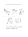
plotNetwork and plotConnections
To visualize connections between cell assemblies, these two functions either draw
a connection matrix or a network graph.
4.4.4 Tools ni.tools - .plot - Plot Functions
38
Figure 4.4.6: Two smooth histograms of a unimodal and a bimodal distribution
as shown with ni.tools.plot.plotHist.
Figure 4.4.7: Visualizations of a random network as a connection matrix and as
a graph.
The graph visualization requires networkx to be installed and normalizes
the weights to the maximum value for each row (or column, depending on the
options set). This forces at least one incoming edge per node and is the default
setting since likelihoods and information criteria are relative to one another only
on the data which they were evaluated on (which is the cell that is influenced,
ergo the likelihoods represent incoming edges). networkx calculates the placement of each node, using the connection strength (which can also be negative)
to perform a spring simulation, minimizing the difference between intended and
actual distance. This placement can be different for each time plotNetwork is
called. Then, connections are drawn using the annotate matplotlib function.
Connections that are higher than 90% of the maximum are drawn as solids,
higher than 50% are drawn as gray dashed lines and all others as light-gray
dotted lines.
The connection matrix that is drawn by plotConnections scales dots to show
connection strength. Connections from a node onto itself are colored differently
(in the example a lighter gray) to make the orientation of the connectivity matrix
easily apparent.
4.4.5 Tools ni.tools - statcollector - Collecting Statistics
4.4.5
39
statcollector - Collecting Statistics
A StatCollector is a data structure that aims to make it easy to collect statistics
about models. Essentially it is a dictionary of dictionaries, where the first level
indexes the model the statistics is about and the second level the different
kinds of values. This seems unintuitive, when one wants to eg. quickly get all
likelihoods. But keeping the model in the top level enables one to filter models
on certain criterion.
import ni
stat = ni.StatCollector()
stat.addNode("Model 0", {’ll_test’: -240,
’ll_train’: -80,
’complexity’:10})
stat.addNode("Model 0/1", {’ll_test’: -100,
’ll_train’: -90,
’complexity’:14})
Figure 4.4.8: An example of a StatCollector instance: “Model 0/1” extends
“Model 0”, which in turn is extended by “Model 0/1/2”. Not all models contain
all values. In [Konishi and Kitagawa, 2007] on page 87 there is a very similar
picture illustrating how adding components to a weather model changes the AIC
of the models.
The name of the node identifies the model. Models that extend other models
can use a pseudo tree structure by including forward slashes in their name.
Values of a specific keyword can be fetched for all models.
StatCollectors allow to filter models either with a prefix string or arbitrary
regular expression. Renaming models is also possible with the rename method.
Model levels can be pushed into attribute names or attribute prefixes pushed
back into model names. Eg. bootstrap evaluations with different data sets will
generate the same attributes. To associate them to the same model, the bootstrap function can prefix the names of the attributes with eg. ’dataset1_’. Alternatively, a new subnode to the model can be created (’Model 0/1/dataset1’),
4.4.6 Tools ni.tools - html view - Collecting and Rendering HTML Output 40
which allows eg. for all test likelihoods to be collected, regardless from which
evaluation they come. If the EIC for different datasets is to be compared
for one model, one can push the last level of the model name into the attribute name: ’Model 0/1/dataset1’ and ’ll_test’ becomes ’Model 0/1’ and
’dataset1_ll_test’.
StatCollectors are useful when one wants to plot distributions of values of
some evaluation for a range of models that relate to one another.
StatCollectors can be saved and loaded to a file. Also a list of files can be
loaded, which are then incorporated into one StatCollector instance. Instead
of a list a glob 6 can be used (a string containing the wild-card character * such
as ’session3/*.stat’), which then loads a list of files that match the pattern.
4.4.6
html view - Collecting and Rendering HTML Output
The hypertext markup language (html) is a very flexible way of setting text
and graphics as interactive or non-interactive websites. It builds on an ordered
tree structure that holds all elements that are to be displayed. The jQuery 7
JavaScript library enables interactive functionalities with few to no lines of
code, from simple hiding and showing of elements to animations and complex
manipulations of the document tree.
The View class offers a simplified tree structure to save output to, which
is then rendered as a fully styled html file. The tree structure is instantiated
by saving objects to certain paths, ie. forward slash separated nodes. If two
elements have exactly the same path, the second object overwrites the first
one, so some unique identifier should be included in the path. These paths are
compiled into an actual tree structure that is parsed by a recursive interpreter,
such that arbitrarily nested output can be generated. In this structure, nodes
are sorted alphabetically8 Some node names have special roles and shift the
interpreter into a different mode:
tabs
The keyword tabs creates a tabbed interface, such that only one of the
children will be displayed at a time. If one tab is selected the focus can
be changed with the arrow keys.
Example ’Cells/tabs/1/plot A’, ’Cells/tabs/2/plot A’ will create two
tabs under the title Cell labeled with 1 and 2 containing the node ’plot A’
for each cell.
hidden
The child will be hidden until a link + show/hide ... is clicked.
table
The children will be displayed in a table, sorted by the next two nodes in
the path as rows and columns.
6 named
after an archaic Unix program
http://jquery.com/
8 with numbers being treated as complete numbers and not digits: 9 < 10 < 100 instead of
10 < 100 < 9
7 see
4.4.6 Tools ni.tools - html view - Collecting and Rendering HTML Output 41
#N
for intergers N changes the order of elements, but is not displayed.
Example: ’Plots/#1/Plot about Zebras’, ’Plots/#2/Plot about Ants’ will
show the Zebra plot before the Ants plot, although normally they would
be sorted alphabetically.
Some objects of the ni. toolbox contain methods that generate a representation of themselves to be inserted into a View. A FittedModel eg. will create
three tabs, one with the configuration options, one with plots of the design components and one with the fitted design components. A Data object will show
the mean firing rates across cells and trials and spike plots in a tabbed interface.
The default StatCollector output is made up out of very broad plots that cover
all possible dimensions that are contained in the object. In most cases only a
few of those plots are informative.
View is a context manager. If it is initialized with a filepath and used in
a with statement, the View will be rendered to this file, even in case of an
exception being raised.
4.4.6.1
Figures in View Objects
Figures can be saved into a View via the .savefig(path, fig) method. It will
insert a png image of the plot, encoded in a base64 string.9 This makes it
possible to have the picture directly embedded in the html file. The image can
be saved or copied from any web browser, but no actual image file is created.
While this reduces clutter files in the output directory, this can also cause the
html file to become as large as a few megabytes and a bit slow to load over a
network if a lot of plots are produced, even if they are hidden in tabs.
The View class also offers a .figure(path) method, that returns a context
manager, such that a new matplotlib figure is created when the context is entered
and this figure is saved in the tree when the context is left.
Like StatCollectors, View can load lists of files or all files matching a wildcart glob pattern.
9 See
http://en.wikipedia.org/wiki/Base64
Chapter 5
Bootstrapping an
Information Criterion
A problem in statistical modeling is to find a good complexity for a model to
predict unseen data most accurately. It is easy to tune a model in such a way
that it has a high likelihood on the training set (or even one additional test
set, if one tweaks in response to test set evaluation), but this may model not
the process in question, but rather the noise in the particular instance of the
process.
When additional free parameters are added to a model, the likelihood will
become greater - or stay at least equal - since if the new parameter does not
explain any previously poorly matched data, it will be just set to 0.
Every model that is obtained by maximum likelihood estimation has a systematic error - a bias - in estimating its own likelihood on training data. This
bias needs to be estimated to find out which model is actually better. One such
method is the Akaike Information Criterion (AIC)1 , another the Bayesian Information Criterion (BIC) and lastly the Extended Information Criterion (EIC).
5.0.7
AIC
The AIC aims to compensate for the bias by taking the number of free parameters into account and adding them as a penalty onto the likelihood. In a set of
models, the best model is that which minimizes the AIC estimation:
𝐴𝐼𝐶(𝑚, 𝑑) = −2𝑙(𝑚, 𝑑) + 2𝑘
(5.1)
Definition from [Akaike, 1973, Akaike, 1974]
𝑚 is a model, 𝑑 is the data and 𝑘 the number of parameters. 𝑙(𝑚, 𝑑) is the log-likelihood
of the data, given the model.
1
or An Information Criterion
42
5.0.8 Tools ni.tools - BIC
43
The AIC is a relative estimate of the information lost when representing
a process by a model. It does not give an absolute measure on how good a
model is (as would hypothesis testing), but rather
a relative [︁comparison.
It is
(︁
{︁
}︁]︁)︁
derived from the Kullback-Leibler divergence 𝐼(𝐺; 𝐹 ) = 𝐸𝐺 log
𝐺(𝑋)
𝐹 (𝑋)
as
described in [Konishi and Kitagawa, 2007]. Since the true distribution is not
known, the KL divergence is simplified to 𝐸𝐺 [log 𝑔(𝑋)] − 𝐸𝐺 [log 𝑓 (𝑋)]. Since
the measure is only used in relativistic terms, the first term (which is equal for
all models that try to approximate 𝑔), can be dropped, leaving only the expected
log-likelihood, which can be approximated with collected data.
In these terms, the best model is the one, which maximizes the log-likelihood
on the observed data. But this estimation is heavily biased, as the model will
always perform well on the data it was trained on. For every finite set of
observed data, the set of parameters 𝜃^ that is obtained by maximum likelihood
estimation, yields an equal or higher likelihood on the observed data than the
parameters of the true distribution, even if the process is indeed identical to the
model.[Konishi and Kitagawa, 2007, p.54] If one assumes that there exists a 𝜃
that makes the model perfectly approximate the process that is to be modeled,
it can be shown that this bias approximates the number of free parameters used
in the model.
The AIC can be used as a model selection method, just like the maximum
likelihood method. Just like the likelihood, AIC changes with the amount of
data used to fit the model. In particular, one might notice that when the
amount of data used to fit a model is rising, the likelihood drops, as more
data means more overall mismatch between data and prediction. But while the
likelihood scales in magnitude with the data, the bias is expected to approximate
closer and closer to the number of parameters. [Shibata, 1976] claims that with
increasing number of observations, even if a more complex model is selected, the
coefficients will be closer to their real value - in case of unnecessary coefficients
0.[Konishi and Kitagawa, 2007, p.74]
5.0.8
BIC
The BIC or Schwarz’s information criterion, uses posterior probability to select
models. This approach is simplified to estimating the marginal probability, since
all other factors in the posterior probability
are equal for all models.
∫︀
The marginal probability is given by 𝑓 (𝑥𝑛 |𝜃)𝜋(𝜃)𝑑𝜃, which is approximated
as:
∫︁
^ + 𝑘 log 𝑛
− 2 log 𝑓 (𝑥𝑛 |𝜃)𝜋𝑖 (𝜃)𝑑𝜃 = −2 log 𝑓 (𝑥𝑛 |𝜃)
(5.2)
𝜋𝑖 (𝜃) is the prior probability of the model with the parameters 𝜃. 𝑘 the number
of parameters, 𝑛 the number of observations. 𝑓 (𝑥𝑛 |𝜃) is the likelihood of the data,
^ the likelihood given the maximum likelihood estimated model.
given the model, 𝑓 (𝑥𝑛 |𝜃)
[Konishi and Kitagawa, 2007, Chapter 9]
The definition of the BIC is very similar to the AIC, but also takes into
5.0.9 Tools ni.tools - EIC
44
account how much data is used for estimating the log-likelihood:
𝐵𝐼𝐶(𝑚, 𝑑) = −2 log 𝑙(𝑚, 𝑑) + 𝑘 log 𝑛
(5.3)
Where 𝑘 is the number of free parameters and 𝑛 the number of observations.
For the amount of observations used in Experiment 1 in 5.1, this will be
quite a significant difference to the factor 2 of the AIC.
5.0.9
EIC
The EIC tries to estimate the bias by sampling from the data and extrapolating
its features, then fitting the model on both, the original (training) and resampled data and estimating how much the training data overestimates its own
likelihood. This can be thought of as an exaggeration of the bias, resulting in
models that are clearly overfitted to an overrepresented feature in the data.
^ obtained by the bootstrap
Using a large number of bootstrap samples d,
transformation T, each giving rise to a fitted model m,
^ the EIC criterion is
calculated by estimating the expected bias as a mean of all bootstrap biases
^ − 𝑙(𝑚, d)
^ to the model 𝑚 fitted on the actual data 𝑑.
𝑙(m,
^ d)
^ − 𝑙(𝑚, d)]
^
𝐸𝐼𝐶𝑇 (𝑚, 𝑑) = −2𝑙(𝑚, 𝑑) + 2[𝑙(m,
^ d)
^ = 𝑇 (𝑑)
d
^
m
^ = 𝑓 𝑖𝑡(d)
(5.4)
^
𝑚 is a model, 𝑑 is the data, m
^ a model fitted on one particular bootstrap sample d,
which was obtained by using 𝑇 on 𝑑. 𝑙(𝑚, 𝑑) is the log-likelihood of the data, given the
model. 𝑇 is a bootstrap transformation.
^
Note that the Data has to be of the same size for 𝑑 and d.
A bootstrap transformation can be a simple jack knife operation that takes
one of the samples out or a a trial based reshuffling of the data. Also one can
re-sample the data from a previously made model.
In [Konishi and Kitagawa, 2007, Chapter 8.3] a Variance Reduction Method
is discussed that was introduced in [KONISHI and KITAGAWA, 1996]. The
extended formula 5.5 (equivalent to [Konishi and Kitagawa, 2007, p.199], equation 8.28) takes into account the difference of the bootstrap model m
^ and the
^ and the actual data 𝑑. This can
actual model 𝑚 on both, the bootstrap data d
result in a faster convergence than only the evaluation on the bootstrap data.
[︁
]︁
^ − 𝑙(𝑚, d)
^ − [𝑙(m,
𝐸𝐼𝐶𝑇 (𝑚, 𝑑) = −2𝑙(𝑚, 𝑑)+2 𝑙(m,
^ d)
^ 𝑑) − 𝑙(𝑚, 𝑑)] ^
d = 𝑇 (𝑑)
^
m
^ = 𝑓 𝑖𝑡(d)
(5.5)
5.0.9 Tools ni.tools - EIC
45
^ and 𝑙(𝑚, d)
^ are the log-likelihood of the bootstrap-sample fitted model and the
𝑙(m,
^ d)
actual data fitted model on the bootstrap sample.
𝑙(m,
^ 𝑑) and 𝑙(𝑚, 𝑑) show the log likelihood of the actual data, given the bootstrap sample/actual data fitted model.
^ − 𝑙(𝑚, d)
^
However, there can be a large asymmetry between the bias 𝑙(m,
^ d)
on the bootstrap data and 𝑙(m,
^ 𝑑) − 𝑙(𝑚, 𝑑) on the normal data, depending on
the transformation.
As a bootstrap transformation, one can reshuffle trials instead of time points,
which will result in less data that is very similar to the original data. In the
following sections, specifically Section 5.1.1.7, the implications of this change are
discussed. Also one can approximate the distribution of spike trains of which
we want to sample more data by a model of varying complexity. This leads to
not a single EIC, but to a range of different criteria that differ in their function
and feasibility (Section 5.0.9.2 will extend on this notion).
The EIC is also used by the R-package reams 2 , which uses a resampling of
observations, for model selection. It uses the leaps exhaustive search regression
fit.
5.0.9.1
Resampling by Creating More Spike Trains
Instead of sampling from instances of time points or complete spike trains, it is
also possible to sample from the probability space of the process that is under
investigation. This requires a model of the process, from which new spike trains
can be generated. This will however also give different results than physically
sampling from the actual process, since the model and the process will diverge
in some aspects. But from this, even more can be inferred about the model, as
the fact that some models have an asymmetric bias compared to the generated
data and others might not, gives insight into whether a model is able to pick up
statistics that are (by their generative process) really present in the data.
5.0.9.2
A Range of Criteria
The EIC can be used with a variety of bootstrap transformations and as one of
two equations. The Equation 5.4 provides the conservative estimation, while 5.5
will reduce the variance and converge faster, but introduce a second source of
variability, which in theory should balance the first, but might behave differently.
As a transformation it is possible to use one of the following methods, resulting in two EIC criteria each:
∙ Resampling based on the original data
∘ redrawing time points
→ conservative EIC using time reshuffle (𝐸𝐼𝐶)
→ variance reduced EIC using time reshuffle (𝑣𝑟𝐸𝐼𝐶)
2 http://cran.r-project.org/web/packages/reams/index.html
5.1 Experiment 1
46
∘ redrawing trials
→ conservative EIC using trial reshuffle (𝐸𝐼𝐶𝑡𝑟𝑖𝑎𝑙𝑠 )
→ variance reduced EIC using trial reshuffle (𝑣𝑟𝐸𝐼𝐶𝑡𝑟𝑖𝑎𝑙𝑠 )
∙ Model based resampling
∘ using simple models
→ conservative EIC using a simple model (𝐸𝐼𝐶𝑠𝑖𝑚𝑝𝑙𝑒 )
→ variance reduced EIC using a simple model (𝑣𝑟𝐸𝐼𝐶𝑠𝑖𝑚𝑝𝑙𝑒 )
∘ using complex models
→ conservative EIC using a complex model (𝐸𝐼𝐶𝑐𝑜𝑚𝑝𝑙𝑒𝑥 )
→ variance reduced EIC using a complex model (𝑣𝑟𝐸𝐼𝐶𝑐𝑜𝑚𝑝𝑙𝑒𝑥 )
This gives rise to 8 kinds of EICs. The model based resampling has a clear
disadvantage in that it needs a fitted model, which extends the computational
requirements by another task. However, it might be that only those models
can provide adequate approximation to the data, such that the EIC produces
meaningful values.
To investigate this, experiments were conducted, calculating each of the EIC
for different bootstrap transformations and comparing the results.
The following table 5.1 gives another overview about the used EIC values:
time based reshuffling
trial based reshuffling
simple Model
complex Model
conservative EIC (Eq. 5.4)
𝐸𝐼𝐶
𝐸𝐼𝐶𝑡𝑟𝑖𝑎𝑙𝑠
𝐸𝐼𝐶𝑠𝑖𝑚𝑝𝑙𝑒
𝐸𝐼𝐶𝑐𝑜𝑚𝑝𝑙𝑒𝑥
variance reduced EIC (Eq. 5.5)
𝑣𝑟𝐸𝐼𝐶
𝑣𝑟𝐸𝐼𝐶𝑡𝑟𝑖𝑎𝑙𝑠
𝑣𝑟𝐸𝐼𝐶𝑠𝑖𝑚𝑝𝑙𝑒
𝑣𝑟𝐸𝐼𝐶𝑐𝑜𝑚𝑝𝑙𝑒𝑥
Table 5.1: Different variants of the EIC. The 𝐸𝐼𝐶 without subscript is the
original definition, while 𝑣𝑟𝐸𝐼𝐶 incorporates the variance reduction method of
[KONISHI and KITAGAWA, 1996]. The variants with subscript describe alternative bootstrap transformations.
5.1
Experiment 1
The bias in the likelihood estimation of likelihood maximized models is systematically higher than the actual likelihood. However it might vary from model
to model and different data statistics. A different model might have a different
bias due to complexity and the nature of the components that make up the
model. Also a model might have a different bias on data with different statistics
as certain regularities in the data might be easier or harder to pick up by the
model. Also the amount of noise that looks like an important property of the
data plays a role, as well as the tendency of the noise to cancel out.
5.1 Experiment 1
47
(a)
(b)
(c)
(d)
Figure 5.1.1: Sets of 50 trials for cell 0 and cell 5: (a) original data (b) Trial
shuffled data, (c) generated with a simple autohistory model and (d) generated
with a complex crosshistory model
Since the kind of bootstrap transformation may lead to different results, five
^ were used (see also 5.1.1). One additional
different kinds of bootstrap data d
bootstrap method to the four mentioned in table 5.1 was used, as by an implementation error the time reshuffle was only performed on the independent, yet
not on the dependent variable. This additional bootstrap data will not contain
the statistical relationship between independent and dependent variables that
the model is supposed to pick up and can act as a control for how important
mimicking the original data actually is.
The experiment uses the following 10 versions of EIC:
∙ time shuffled data (𝐸𝐼𝐶 and 𝑣𝑟𝐸𝐼𝐶)
∙ trial shuffled data (𝐸𝐼𝐶𝑡𝑟𝑖𝑎𝑙𝑠 and 𝑣𝑟𝐸𝐼𝐶𝑡𝑟𝑖𝑎𝑙𝑠 )
∙ data, in which the relationship between independent and dependent variable is destroyed (conservative EIC using unrelated data (𝐸𝐼𝐶𝑢𝑛𝑟𝑒𝑙𝑎𝑡𝑒𝑑 )
and variance reduced EIC using unrelated data (𝑣𝑟𝐸𝐼𝐶𝑢𝑛𝑟𝑒𝑙𝑎𝑡𝑒𝑑 ))
∙ data generated by a simple model (𝐸𝐼𝐶𝑠𝑖𝑚𝑝𝑙𝑒 and 𝑣𝑟𝐸𝐼𝐶𝑠𝑖𝑚𝑝𝑙𝑒 )
∙ data generated by a complex model (𝐸𝐼𝐶𝑐𝑜𝑚𝑝𝑙𝑒𝑥 and 𝑣𝑟𝐸𝐼𝐶𝑐𝑜𝑚𝑝𝑙𝑒𝑥 )
5.1.1 Experiment 1 - Results
48
Of each kind of bootstrap data 50 sets of 50 trials of newly generated data
were created. Two multi channel models were fitted on the dataset, one using
rate and autohistory and one additionally using higher order autohistory and
full crosshistory components. Each of these models then generated 50×50 trials,
which were saved into files.
Trial and time shuffling was done on-the-fly, without generating and saving
data to the network storage, which has the effect that the trials will have a
different order for all evaluations. In contrast the generated data will have the
same order of trials for all evaluations.
Then models were created, modeling one out of the 11 neurons, once only
with their own autohistory, then with each of the other cells, then with each
ordered pair of other cells, yielding 737 models3 . Each model was bootstrap
^ half of the data as training and half as test data.
evaluated with d,
The experiments were run on the IKW grid with a maximum of 100 jobs
submitted at a time. The fitting of the bootstrap models was done in one job per
cell to fit, as these computations are independent. The generation of 50 trials
each was also done in parallel. Bootstrapping was done as one job for each
model, as the evaluation has to fit the model on original data first to compare it
to the bootstrap fitted models. To only fit the model on the original data once,
it was necessary to run each evaluation as one job.
The resulting information criteria were used to infer connections by calculating the information gain from the simple model to a model containing a certain
cross-component. This gain was then thresholded with 90% of the maximal gain
to show differences in how the information criteria evaluate each interaction.
The source code for this experiment can be found in the toolbox as an
example project.
5.1.1
Results
5.1.1.1
Fitted Multi-Model
The model that generated the simple data is visualized in 5.1.2 and the one for
the complex data in 5.1.3.
3 11 autohistory models +11 × 10 with one crosshistory component +11 × (11 + 10*9 ) with
2
two history components
5.1.1 Experiment 1 - Results
(a) Rate Components
49
(b) Autohistory components
Figure 5.1.2: Components of the created simple model: (a) the rate components
(b) the autohistory components
(a) Rate Components
(b) Autohistory components
(c) Crosshistory components (same scale across all plots)
Figure 5.1.3: Components of the created complex model: (a) the rate components show some fluctuations that are equal for the different cell assemblies.
Some assemblies seem to have a lower firing rate overall. (b) in the autohistory
components there is generally a positive interaction, similar to the exponential
decay in the interspike interval histogram of the data. Some assemblies show an
initial inhibition. (c) shows that some cells are strongly driven by other cells.
There seems to be little negative correlation. The 2d autohistory is not shown.
5.1.1 Experiment 1 - Results
5.1.1.2
50
Information Criteria
How the different criteria evaluate models relative to one another can be seen
best in tree plots4 , which take the simpler models as roots from which the more
complex models evolve - either from left to right or from right to left. The
vertical axis represents one of the information criteria, such that if a model
improves on its predecessor, it will be higher up, if it is worse, it will be lower.
The lines connecting the models are either solid or dashed, depending on
which model they come from, such that in the third level each model receives
two lines: one dashed, one solid.
On the next few pages a few of those figures are drawn which are afterwards
discussed.
To make comparison a bit easier, some plots are plotted from left to right,
others from right to left in complexity, such that two comparable trees can be
seen as mirror images.
4 actually
they more or less resemble the structure of a partially ordered set/lattice
5.1.1 Experiment 1 - Results
51
(a) Likelihood on the training data is (b) Likelihood on the test data sometimes
steadily increasing
increases, but also decreases
Figure 5.1.4: The likelihood behaves differently for unseen data, than for the
data the model was trained on. The plots highlight three models, rising in
complexity. The dotted line is rising confidently for the training data, and for
the test data, each added component also increases likelihood. The dashed line
also rises strictly monotone for the training data, however on the test data the
first component provides an increase, while the second results in a decrease in
test data likelihood, which brings it below the level of likelihood of the initial
model without both components. The solid line is rising higher than the dashed
line in the training data, but on the test data it performs worse and worse with
both components added.
5.1.1 Experiment 1 - Results
(a) negative 𝑣𝑟𝐸𝐼𝐶𝑐𝑜𝑚𝑝𝑙𝑒𝑥
52
(b) negative AIC
(c) test loglikelihood
Figure 5.1.5: comparing an EIC (𝑣𝑟𝐸𝐼𝐶𝑐𝑜𝑚𝑝𝑙𝑒𝑥 ), AIC and test likelihood for
Models on cell 5. See Section 5.1.1.3 and following for a discussion.
(a) negative 𝑣𝑟𝐸𝐼𝐶𝑐𝑜𝑚𝑝𝑙𝑒𝑥
(b) negative AIC
(c) test loglikelihood
Figure 5.1.6: comparing an EIC (𝑣𝑟𝐸𝐼𝐶𝑐𝑜𝑚𝑝𝑙𝑒𝑥 ), AIC and test likelihood for
Models on cell 10. See Section 5.1.1.3 and following for a discussion.
5.1.1 Experiment 1 - Results
5.1.1.3
53
A First Look at the Information Criteria
Since the EIC was bootstrapped, it is interesting to know, how much variance is
to be expected after a certain number of bootstrap samples are drawn. Figure
5.1.7 shows for two cells how the EIC (for the complex generated data) for all
models changes less and less with each new bootstrap sample. Comparing the
changes per sample with the scale of the values in the examples, the changes
becomes negligible for the comparison of most of the models. Also the models
tend to move together for the most part, so even a large change for one model
might also affect all other models to move in the same direction.
Inspecting a tree view of the models,
one can easily see, that with increasing
complexity, the likelihood on the training
data increases as well (see Figure 5.1.4a).
This is plausible, as adding new components can not make the model perform
worse if the likelihood is maximized. It
would be ignored, if it added no new explanatory value, but as it most likely will
increase the fit in some way, the likelihood
is steadily rising.
However, if we consider the likelihood
of the models on previously unseen data,
we get a different picture. Some mod- Figure 5.1.7: Two examples of
els perform better than their less complex how the mean EIC converges (here
predecessors, but just as many perform 𝑣𝑟𝐸𝐼𝐶𝑐𝑜𝑚𝑝𝑙𝑒𝑥 ): The changes of the
worse (see Figure 5.1.4b). This is caused mean with every new bootstrap trial
by the models modeling not an essential get smaller and smaller.
part of the data, but a non-informative
noise part. The models are over-fitting. The apparent good fit on the training
set is only due to the bias of likelihood estimation with maximum likelihood
estimated models.
If one takes the likelihood on the test data as an unbiased “ground truth”, the
information measures EIC and AIC can be compared in how they compensate
the bias on the training data. Figures 5.1.5 and 5.1.6 show how different models
perform on the test data and in each information criteria. EIC and AIC are
shown as negatives, such that a higher value signifies a better model.
5.1.1.4
AIC
It is notable that AIC seldom compensates strongly enough that the least complex model (using only rate and autohistory) can compete with the more complex models. However the simple model seems to be close to the mean performance for cells 0,3,9 and 10, while 2,4,6,7 having it near the mean of the
poor performing models. Only on cells 1,5 and 8 the simplest model is among
the worst models performing on the test data. The AIC however consistently
5.1.1 Experiment 1 - Results
54
Figure 5.1.8: negative AIC of the models for cell 1 and 5
underestimates the simpler models.
5.1.1.5
BIC
Figure 5.1.9: negative BIC of the models for cell 1 and 5
The BIC compensates very strongly for complexity. The simplest model is
in the upper half of models almost always. For cell 3 and 10, it even is the best
chosen model. Figure 5.1.9 shows two examples of how strongly the BIC tilts
the training likelihood plot compared to Figure 5.1.8. The increase in likelihood
for the cell 5 model 5/3/5 to 5/3/5/7, which is a big improvement for the AIC,
is judged to not outweigh the increase in complexity by the BIC.
5.1.1 Experiment 1 - Results
5.1.1.6
55
EIC
The EIC tends to compensate well for the complexity and often5 has an almost
equal split of more complex models enhancing and worsening the simpler model.
Spreading out in the hierarchy, one notices that if two models are evaluated
as quite good, their “offspring” model (incorporating all components of the
previous models) has an even better EIC. It seems that the information gain
from the simple model to the first crosshistory component can be translated
roughly to that from the first to the second crosshistory component, which,
however, is a property that seems to carry from the likelihood on the training
data, rather than the bias correction.
In the following, we have to differentiate the different distributions that were
used for drawing bootstrap samples.
5.1.1.7
𝑣𝑟𝐸𝐼𝐶 - Trial Reshuffling vs. Time Reshuffling
The trial shuffled 𝑣𝑟𝐸𝐼𝐶𝑡𝑟𝑖𝑎𝑙𝑠 compensated for complexity, but not as strongly as the BIC. For most cells,
it signifies only one to two interactions as improving
on the simple model. For cell 2, 5, 8 and 9, the best
model has only one crosshistory component. Those
would hint at a causal interaction 0 → 2, 3 → 5,
10 → 8, 10 → 9.
Cells 1, 3, 4, 6 and 7 give the best EIC value to
a double crosshistory, while 0 and 10 rate the simple model as worse than at least three crosshistory Figure 5.1.10: an inferred graph from EIC
models.
An example of a graph that might be inferred by with trial shuffling
model selection of the EIC with trial reshuffling can
be seen in Figure 5.1.10
5 when
exactly will be discussed shortly
5.1.1 Experiment 1 - Results
(a) Time Reshuffle (𝑣𝑟𝐸𝐼𝐶)
56
(b) Trial Reshuffle (𝑣𝑟𝐸𝐼𝐶𝑡𝑟𝑖𝑎𝑙𝑠 )
(d) Simple Model (𝑣𝑟𝐸𝐼𝐶𝑠𝑖𝑚𝑝𝑙𝑒 )
(c) Unrelated (𝑣𝑟𝐸𝐼𝐶𝑢𝑛𝑟𝑒𝑙𝑎𝑡𝑒𝑑 )
(e) Complex Model (𝑣𝑟𝐸𝐼𝐶𝑐𝑜𝑚𝑝𝑙𝑒𝑥 )
Figure 5.1.11: The variance reduced EIC biases (and only the biases) for cell
10. While the AIC bias would be just a straight line, the EIC calculates the
bias on the basis of the bootstrap distribution, which is why the scale is very
different for all shown examples: The maximal bias correction for (a) is -60,
for (b) it’s about the same, for (c) -800, for (d) it’s -400 and for (e) -120. The
lowest bias (in all cases the simplest model) is for (a) -37, (b) -33, (c) about
-600, (d) -52 and for (d) -40. Not only do the ranges of bias correction differ, the
actual models that get a higher or lower correction is also different for each EIC
version. For the simple and complex model EIC, this means that more complex
models can actually receive a lower bias correction than a particularly bad less
complex model, in some cases even if the more complex one is an extension of
the simpler model (see the dashed line going back up from Model 10/7/10 in
(d) ).
5.1.1 Experiment 1 - Results
5.1.1.8
57
𝑣𝑟𝐸𝐼𝐶𝑠𝑖𝑚𝑝𝑙𝑒 - The Simple Model
The simple model generated data produces the best 𝑣𝑟𝐸𝐼𝐶𝑠𝑖𝑚𝑝𝑙𝑒 for the simple model. This is no surprise, as this model essentially created the data, so
additional parameters can hardly add any explanatory value.
Some models trained on cell 4, 6 and 7 are judged
as almost as good as the simple model. But Model
4/4/6 (having 4 as autohistory and cell 6 as a crosshistory component), while being highly praised by evaluation on the test data, is considered a bad model by
the 𝑣𝑟𝐸𝐼𝐶𝑠𝑖𝑚𝑝𝑙𝑒 . The Model 6/4/6 on cell 6 also has
a very high likelihood on the test data, but is regarded
by the 𝑣𝑟𝐸𝐼𝐶𝑠𝑖𝑚𝑝𝑙𝑒 as pretty bad.
The simple model did not model any crosshistory,
so any relation between the spikes in 4 and 6 in the
bootstrap data can only be a correlation due to firing
rate (eg. mutual fluctuations). However in the real
data, there might be an actual causal relation. This
leads the variance reduction term of the 𝑣𝑟𝐸𝐼𝐶𝑠𝑖𝑚𝑝𝑙𝑒
to penalize this model with a large bias, as the real
model is far better at predicting the actual data and
the term −[𝑙(m,
^ 𝑑) − 𝑙(𝑚, 𝑑)] will be very large (ie.
positive, adding to the penalty).
Figure 5.1.12: conservaIf the EIC would have been calculated by Equation tive 𝐸𝐼𝐶𝑠𝑖𝑚𝑝𝑙𝑒
5.4, the models 4/4/6 and 6/4/6 would far outperform
the simpler model (as seen in the conservative 𝐸𝐼𝐶𝑠𝑖𝑚𝑝𝑙𝑒 plot 5.1.12).
But since the 𝑣𝑟𝐸𝐼𝐶𝑠𝑖𝑚𝑝𝑙𝑒 reduces variance using both directions, the divergence between bootstrap data and real data results in a very large bias being
calculated for these actually good models on the basis of using the simple model
as a bootstrap mechanism.
This divergence between the test data likelihood and EIC estimates also hints
at the fact that important structure in the data is lost, if the sampling process
ignores all cross-causalities. This however is not an insight about the models
being tested, but about the bootstrap data and the model that generated it.
5.1.1.9
𝑣𝑟𝐸𝐼𝐶𝑐𝑜𝑚𝑝𝑙𝑒𝑥 - The Complex Model
The 𝑣𝑟𝐸𝐼𝐶𝑐𝑜𝑚𝑝𝑙𝑒𝑥 computed with the complex model seems to split the models
relative equally in good and bad additions to the model. Some components
improve the 𝑣𝑟𝐸𝐼𝐶𝑐𝑜𝑚𝑝𝑙𝑒𝑥 value significantly. A good component added to a
good model will give an even better model, while components that tend to
overfit reduce the 𝑣𝑟𝐸𝐼𝐶𝑐𝑜𝑚𝑝𝑙𝑒𝑥 value.
5.1.1.10
The EIC Bias
Figure 5.1.11 shows how the different EIC biases are distributed. With rising
complexity, the bias that is corrected also increases. However in contrast to the
5.1.1 Experiment 1 - Results
58
AIC, the bias of each model depends heavily on the statistics on which it was
evaluated.
The trial reshuffled 𝑣𝑟𝐸𝐼𝐶𝑡𝑟𝑖𝑎𝑙𝑠 gives a distribution such that the increase
in bias from the simple model is spread in a range from 7 to 17. The spread
is roughly maintained one complexity level further. But some models even The
𝑣𝑟𝐸𝐼𝐶𝑐𝑜𝑚𝑝𝑙𝑒𝑥 computed on the complex model has a wider spread, and keeps
spreading further, while some models get a smaller bias with the inclusion of an
additional component.
5.1.1.11
Information Gain and Network Inferences
The different information measures give different weight to the simple model.
This gives insight in whether the criterion thinks that a certain interaction
component can improve the model or whether it will lead to over fitting. If
the more complex model has a better value than the simple model, there is an
information gain in including this component in the model.
The gain can be thought of as a split in the tree plots along a line going
through the simple model horizontally.
Gain of:
Training likelihood
Test likelihood
AIC
BIC
conservative EIC reshuffle trials
conservative EIC reshuffle time
conservative EIC reshuffle unrelated
conservative EIC simple model
conservative EIC complex model
variance reduced EIC reshuffle trials
variance reduced EIC reshuffle time
variance reduced EIC reshuffle unrelated
variance reduced EIC simple model
variance reduced EIC complex model
≤0
0
47
37
95
58
67
43
37
44
38
52
104
110
65
>0
110
63
73
15
52
43
67
73
66
72
58
6
0
45
percentage split
0 / 100%
43 / 57%
34 / 66%
86 / 14%
53 / 47%
60 / 40%
39 / 61%
34 / 66%
40 / 60%
35 / 65%
47 / 53%
95 / 5%
100 / 0%
59 / 41%
Table 5.2: Number of connections with a non-positive and positive gain for the
different information criteria. A gain smaller than 0 means that the information
criterion prefers the simpler model to the more complex model. The conservative EIC is calculated by Equation 5.4, while the variance reduced 𝑣𝑟𝐸𝐼𝐶 is
calculated by Equation 5.5
Figures 5.1.13a and 5.1.13b show a thresholded network inference from only
the likelihood of the test data and training data. The graph using the (unbiased) likelihood on the test data should act as a guideline when interpreting
the other graphs. The graph of the likelihood on the training data assumes
a larger gain (since it is biased towards more complex models), which means
that all connections are included. Because of the scaling only the highest connections are plotted as black solid lines to make them comparable to the other
5.1.1 Experiment 1 - Results
59
plots. The training likelihood, after setting a threshold, detects four networks:
{0, 1, 2}, {3, 5}, {4, 6, 7} and {8, 9, 10}.
In the likelihood estimation with unseen test data, the groups {0, 1, 2}, {3, 5}
and {4, 6, 7} are also found, the group {8, 9, 10} however is deemed to be less
connected. Some new connections are inserted as also very beneficial, connecting
cell 2 to 1 and to 9 and 5 to 8.
The AIC finds the same networks as the training likelihood. This is because
the AIC is only bias correcting for complexity, which does not change the order
of the models. Some of the models that had a low gain in the graph 5.1.13b are
now excluded as their gain in likelihood is less than the AIC bias of adding a
crosshistory component.
The BIC selects only a few connections as having a positive gain (Figure
5.1.13d). From the grouping of the nodes it becomes apparent that some of
the connections have a quite large negative gain, separating the nodes into two
assemblies, which are in itself not well connected.
The trail reshuffling 𝑣𝑟𝐸𝐼𝐶𝑡𝑟𝑖𝑎𝑙𝑠 finds essentially the same subnetworks as
the trainings likelihood, however the threshold is lowered a bit as the significant
models are grouped closer together.
Figure 5.1.14d shows how the 𝑣𝑟𝐸𝐼𝐶𝑠𝑖𝑚𝑝𝑙𝑒 depending on the simple model
disregards all connections as not providing any additional information.
5.1.1 Experiment 1 - Results
60
(a) Test likelihood
(b) Trainings likelihood
(c) AIC
(d) BIC
Figure 5.1.13: Networks inferred by different information criteria. The number
of connections can be seen in Table 5.2. It ranges from full connection (even if
only a few are drawn bold) in 5.1.13b to no connections for 5.1.14d.
5.1.1 Experiment 1 - Results
61
(a) 𝑣𝑟𝐸𝐼𝐶 sampling timepoints(b) 𝑣𝑟𝐸𝐼𝐶𝑡𝑟𝑖𝑎𝑙𝑠 sampling trials (c) 𝑣𝑟𝐸𝐼𝐶𝑢𝑛𝑟𝑒𝑙𝑎𝑡𝑒𝑑 sampling unrefrom the data
from the original data
lated to the data
(d) 𝑣𝑟𝐸𝐼𝐶𝑠𝑖𝑚𝑝𝑙𝑒 sampling from the simple (e) 𝑣𝑟𝐸𝐼𝐶𝑐𝑜𝑚𝑝𝑙𝑒𝑥 sampling from the commodel
plex model
Figure 5.1.14: Networks inferred by different information criteria. The number
of connections can be seen in Table 5.2. It ranges from full connection (even if
only a few are drawn bold) in 5.1.13b to no connections for 5.1.14d.
5.1.1 Experiment 1 - Results
62
(a) 𝐸𝐼𝐶 sampling timepoints (b) 𝐸𝐼𝐶𝑡𝑟𝑖𝑎𝑙𝑠 sampling trials from the (c) 𝐸𝐼𝐶𝑢𝑛𝑟𝑒𝑙𝑎𝑡𝑒𝑑 sampling unrefrom the data
original data
lated to the data
(d) 𝐸𝐼𝐶𝑠𝑖𝑚𝑝𝑙𝑒 sampling from the simple (e) 𝑣𝑟𝐸𝐼𝐶𝑐𝑜𝑚𝑝𝑙𝑒𝑥 sampling from the commodel
plex model
Figure 5.1.15: Networks inferred by the simple version of the EIC. The trial
shuffled EIC looses connections (compare to 5.1.14b). All other versions of the
EIC gain more connections. This evaluation however might not be saturated,
as the simple version of the EIC needs longer to converge.
5.1.2 Experiment 1 - Discussion
5.1.2
63
Discussion
AIC tries to compensate only for complexity as the length of the coefficients
vector. If this could be used reliably for model selection (even with arbitrary
weights of how much complexity should be weighted), models of one complexity
class would remain in their order after bias correction. However, different models
have different biases on different data, as shown by simple cross evaluation.
When using the bias corrected likelihood on the training data as a network
inference technique, the differences in the order of models is very small. Only
the decision which connections to include at all can be assisted with with the
different information criteria.
There is a very large difference in the behavior of the trial-shuffled and
the time-shuffled 𝑣𝑟𝐸𝐼𝐶 and the unrelated shuffling 𝑣𝑟𝐸𝐼𝐶𝑢𝑛𝑟𝑒𝑙𝑎𝑡𝑒𝑑 . This can
be expected to some extend, as the unrelated shuffle destroys the statistical
properties of the data, while the trial or time point shuffle preserves it. In fact
for the connectivity plots, 𝑣𝑟𝐸𝐼𝐶𝑢𝑛𝑟𝑒𝑙𝑎𝑡𝑒𝑑 behaves very similar to the simple
model 𝑣𝑟𝐸𝐼𝐶𝑠𝑖𝑚𝑝𝑙𝑒 . Both take the simple model to be most robust and hence
discard assumptions connectivity.
Yet, the 𝐸𝐼𝐶𝑢𝑛𝑟𝑒𝑙𝑎𝑡𝑒𝑑 does show connectivity, as does 𝐸𝐼𝐶𝑠𝑖𝑚𝑝𝑙𝑒 . Although
there was no statistics in the bootstrap data, that would hint at the connectivity,
Equation 5.4 seems to be robust enough to still provide meaningful values. In
Section 6.2 this will be discussed further.
5.2
Experiment 2 - Using Information Criteria
for Parameter Selection
To give another application to information criteria, consider the common case
of answering the question how many basis splines should be used to model the
rate fluctuations in a certain set of data. Normally, one would use a simple
cross evaluation for this. However, if data is precious (eg. if some further model
selection process requires fresh data as bootstrapping is not possible), one has
to resort to using transformed versions of the training data and compensate for
the bias as good as one can.
The source code for this experiment can be found in the toolbox as an
example project.
5.2.1
Results
The models up to 100 knots get continually better. This can be seen in the
test data likelihood plot in Figure 5.2.1a. It may be interesting that the linearly
spaced rate component seems to fit the data better than the adaptive rate, which
might hint at an error in the implementation, or it might be the case that for
this set of data, the resolution should not be scaled with the firing rate. But for
the comparison of information criteria even a defective adaptive rate component
can be useful, as we know the likelihood of those models on test data.
5.2.1 Experiment 2 - Using Information Criteria for Parameter Selection Results
64
(a) Test likelihood
(c) 𝑣𝑟𝐸𝐼𝐶𝑡𝑟𝑖𝑎𝑙𝑠
(b) Training likelihood
(d) AIC
(e) BIC
Figure 5.2.1: This experiment shows how the information criteria can be used
to find an optimal parameter such as the number of knots of a rate component.
The training likelihood rises continually while the test likelihood falls again
after 100 knots. The goal is to find an information criterion that will identify
the bias such that the maximum in test likelihood coincides with an optimum
in the information criterion.
The BIC has a global minimum for the lin-spaced rate at 50 knots, with 100
knots being evaluated as second best. For the adaptive rate, there is a plateau
for the small knot numbers and a worsening after 50 knots.
The AIC finds a minimum for the adaptive rate at 100 knots, for the linspaced rate a plateau after 100 knots implies an equal weight off between likelihood gained and complexity.
For the EIC values, one has to differentiate again. 𝑣𝑟𝐸𝐼𝐶𝑡𝑟𝑖𝑎𝑙𝑠 shows a
strong divergence between adaptive and lin-spaced rate models. The adaptive
models are judged similar to the BIC, the lin-spaced models similar to the AIC.
The 𝐸𝐼𝐶𝑡𝑟𝑖𝑎𝑙𝑠 and 𝐸𝐼𝐶𝑐𝑜𝑚𝑝𝑙𝑒𝑥 show a large amount of variance, such that
local minima can not really be interpreted. 𝐸𝐼𝐶𝑐𝑜𝑚𝑝𝑙𝑒𝑥 has a large global minimum for the lin-spaced rate models around 100 knots. 𝑣𝑟𝐸𝐼𝐶𝑐𝑜𝑚𝑝𝑙𝑒𝑥 in contrast
only shows an even stronger plateau behavior than the BIC. The 𝑣𝑟𝐸𝐼𝐶𝑠𝑖𝑚𝑝𝑙𝑒
is almost equivalent to 𝑣𝑟𝐸𝐼𝐶𝑐𝑜𝑚𝑝𝑙𝑒𝑥 . This might be due to the models that
generated the data having a very low number of knots.
5.2.2 Experiment 2 - Using Information Criteria for Parameter Selection Discussion
65
(c) 𝐸𝐼𝐶𝑐𝑜𝑚𝑝𝑙𝑒𝑥
(a) 𝐸𝐼𝐶𝑡𝑟𝑖𝑎𝑙𝑠
(b) 𝑣𝑟𝐸𝐼𝐶𝑡𝑟𝑖𝑎𝑙𝑠
(d) 𝑣𝑟𝐸𝐼𝐶𝑐𝑜𝑚𝑝𝑙𝑒𝑥
(e) 𝐸𝐼𝐶𝑠𝑖𝑚𝑝𝑙𝑒
(f) 𝑣𝑟𝐸𝐼𝐶𝑠𝑖𝑚𝑝𝑙𝑒
Figure 5.2.2: The differences in how the different EIC values punish complexity
shows very different evaluations. Some (eg. 𝐸𝐼𝐶𝑐𝑜𝑚𝑝𝑙𝑒𝑥 ) find a clear global
minimum, others (𝑣𝑟𝐸𝐼𝐶𝑐𝑜𝑚𝑝𝑙𝑒𝑥 ) see the optimum with having as few splines
as possible. 𝐸𝐼𝐶𝑡𝑟𝑖𝑎𝑙𝑠 might even suggest that an even higher complexity might
not be detrimental to the model.
5.2.2
Discussion
The test likelihood gave a very clear indication when over fitting is occurring,
namely after adding more than 100 knots. In the training likelihood this is
noticeable by the decreased in incline after 100 knots. This means, that an
arbitrary penalty factor 𝛼 of complexity exists for this particular set of models,
such that
𝐼𝐶(𝑚, 𝑑) = −2 · 𝑙(𝑚, 𝑑) + 𝛼𝑘
(5.6)
𝐼𝐶 is some information criterion, 𝑙(𝑚, 𝑑) is the log-likelihood of the model, 𝑘 is the
number of parameters.
will give an optimum at the maximal test likelihood. However, this penalty
factor might be different for the adaptive rate models and the linearly spaced
rate models.
The AIC has a penalty factor of 𝛼 = 2 and finds the optimum of the adaptive
rate model. The BIC has a factor of 𝛼 = 𝑙𝑜𝑔(3300) = 8.1 and finds the optimum
of the linearly spaced models. This means that a penalty factor multiplied with
the complexity of the models might not find both optima at once. An 𝛼 of 4
might, but this would be an a-posteriori tuning of the parameter without any
5.2.2 Experiment 2 - Using Information Criteria for Parameter Selection Discussion
66
(a) 𝐸𝐼𝐶𝑐𝑜𝑚𝑝𝑙𝑒𝑥
(b) 𝑣𝑟𝐸𝐼𝐶𝑐𝑜𝑚𝑝𝑙𝑒𝑥
Figure 5.2.3: The progression of EIC converging to its value used in Figure
5.2.2. The 𝑣𝑟𝐸𝐼𝐶 converges quicker, but for the conservative 𝐸𝐼𝐶 there is not
much movement to be expected either.
theoretical justification, purely on the basis on what we know would lead to a
good result.
Independent of whether there is or is no optimum of number of knots, we
can ask, whether having too few or too many knots will make our model worse.
The AIC would say, a small number of knots will give worse models, above 100
they are about equally good, while the BIC would say that below 30 are good
models, 50 is even a bit better, but after that the model will be worse by far.
The EIC criteria, eg. the 𝑣𝑟𝐸𝐼𝐶𝑡𝑟𝑖𝑎𝑙𝑠 will give different answers for the
adaptive and lin-spaced rate models. For the adaptive rate, higher number of
knots are bad6 (similar to BIC), for the lin-spaced rate, more knots are generally
not bad, but also do not improve the model (similar to AIC).
That 𝑣𝑟𝐸𝐼𝐶𝑐𝑜𝑚𝑝𝑙𝑒𝑥 and 𝑣𝑟𝐸𝐼𝐶𝑠𝑖𝑚𝑝𝑙𝑒 show no improvement after 30 knots
is probably due to their own models having a very low number of knots. Although the 𝑣𝑟𝐸𝐼𝐶𝑐𝑜𝑚𝑝𝑙𝑒𝑥 model is named complex, it is actually not that complex when seen from the perspective of the rate models, which are not interested in crosstalk between the neuron assemblies. However, the 𝐸𝐼𝐶𝑐𝑜𝑚𝑝𝑙𝑒𝑥 and
𝐸𝐼𝐶𝑠𝑖𝑚𝑝𝑙𝑒 find an optimum at around 100 knots, which coincides with the test
likelihood.
So, somehow the conservative EIC can utilize data fluctuations to estimate
a bias that comes close to the test likelihood, while for the 𝑣𝑟𝐸𝐼𝐶 the difference
between fluctuations and the real data create a bias that effectively inverts the
training likelihood.
This might be explainable by the uninformative nature of the bootstrap data:
The data that was generated by the low-knot-number models did not allow the
models to learn about the actual structure of the data, such that even models
with a high number of rate knots only emulated the low-knot fluctuations. When
compared to the actual model, all models had roughly the same 𝑙(m,
^ 𝑑), as it at best - emulated the rate function of the generative model. As the complexity
of the model rises, the bias gets larger as the actual model is able to predict the
data more accurately, while the bootstrap models remain at some fixed level.
6 which
is plausible, should the adaptive rate component indeed be defective
5.2.2 Experiment 2 - Using Information Criteria for Parameter Selection Discussion
67
The bias rises with the likelihood gained on training data, as this is what the
𝑙(m,
^ 𝑑) term is compared to.
The bias correction of the 𝐸𝐼𝐶𝑐𝑜𝑚𝑝𝑙𝑒𝑥 and 𝐸𝐼𝐶𝑠𝑖𝑚𝑝𝑙𝑒 does not contain this
large term and is therefore less influenced by the inverse shape of the training
likelihood.
Chapter 6
Conclusions
The prospects of using a sampling method to provide an unbiased model evaluation criterion on the basis of training data is promising a lot. If successful,
cross-evaluation will no longer be needed and more data can be used for fitting,
creating better models. Also an arbitrarily large number of model-selection processes can be included in the fitting process, with each having full access to the
data.
But can the methods described in this thesis actually deliver what they
promise?
6.1
The Differences between AIC, BIC and EIC
As expected, the AIC bias correction is a very static way to balance complexity
of the model. It does not take the data into account or the nature of the
components that make the model more complex. From the likelihood on test
data, we know that the bias is not static and different models on different data
will overestimate its likelihood in differing amounts.
The BIC showed very sparse results for Experiment 1, judging the simpler
model a lot better than most other criteria. In Experiment 2 it also penalized
the complexity more than the other criteria, which lead to it identifying a potential optimum for the number of knots. However this could also be a false
positive. As the trial length gives a large number of observations, the complexity is harshly punished by the BIC1 . While it was initially only included as the
model backends calculated it anyway, it seems an interesting subject for further
studies.
For the EIC the outcome relies heavily on what bootstrap transformation is
used. Whether data is drawn from the original data, whether as trials or time
points, or whether a model was used to create new bootstrap data. Also the
two definitions of EIC in Equations 5.4 and 5.5 give different results. In the
following sections those options will be compared.
1 𝑙𝑜𝑔(3300)
≈ 8.1, which results in a four times as large bias as the AIC
68
6.2 The Difference between Conservative and Variance Reduced EIC
6.2
69
The Difference between Conservative and
Variance Reduced EIC
While the variance reduced 𝑣𝑟𝐸𝐼𝐶 can be regarded as a simple extension of
the original definition that will converge earlier, Experiment 1 has shown that
it also behaves very differently when bootstrap data and real data diverge in
their statistics.
It might very well be, that a degenerate transformation of the data (eg.
unrelated resampling) will result in a usable conservative 𝐸𝐼𝐶, it will certainly
give a very intense bias for the variance reduced 𝑣𝑟𝐸𝐼𝐶. This is because the
term to calculate the bias in the conservative Equation only relies on actual
^ − 𝑙(𝑚, d)
^ will contain the biased likelihood minus
data and the term 𝑙(m,
^ d)
how likely that data is for a normally fitted model.
The inverse term that is used for faster convergence however also includes
the likelihood differences on the original data 𝑙(m,
^ 𝑑) − 𝑙(𝑚, 𝑑), which for a
degenerate model will be far off from the actual model. As the model will
generally be better at predicting the actual data, 𝑙(𝑚, 𝑑) will be closer to 0 than
𝑙(m,
^ 𝑑). As log-likelihoods are negative, the term −[𝑙(m,
^ 𝑑) − 𝑙(𝑚, 𝑑)] will be
very positive, adding to the bias.
The conservative 𝐸𝐼𝐶 from Equation 5.4 uses the data only to
draw biased models from a larger variety of data, while the variance
reduced version also uses the greater variance in the reverse term,
which makes it essential for the variance reduced version of the EIC,
that the actual and the bootstrap data are not too far off.
Also in Experiment 2, the consequences of uninformative bootstrap data
could be seen. It will result in the actual model projecting its own training
likelihood (including bias) as a bias correction, as the bootstrap models are
equally bad at predicting the actual data.
6.2.1
The Difference between Trial Based and Time Based
Resampling for EIC
The difference of time based 𝑣𝑟𝐸𝐼𝐶 and trial based 𝑣𝑟𝐸𝐼𝐶𝑡𝑟𝑖𝑎𝑙𝑠 is not a huge
one, as can be expected. A few models may be regarded a tiny bit better by
one or the other, but especially for those models, that greatly benefit from a
certain connection, this does not interfere at all.
The 𝐸𝐼𝐶 versions differ a bit more, but also not to an extend that would
change the connectivity plots. For cell 4 eg. the 𝐸𝐼𝐶𝑡𝑟𝑖𝑎𝑙𝑠 takes Model 7/4/7
and 7/6/7 to be very close, while 𝐸𝐼𝐶, as well as AIC and BIC, see Model
7/4/7 as significantly superior to 7/6/7.
It might be that the 𝐸𝐼𝐶 did not converge enough for the time point resampling to show meaningful results. All values are fairly close together compared
to the variance of the cumulative mean. The inverse term in the 𝑣𝑟𝐸𝐼𝐶 did,
in contrast to the model based resampling, compute a useable bias, excluding
30-50% of the connections. The conservative 𝐸𝐼𝐶 and 𝐸𝐼𝐶𝑡𝑟𝑖𝑎𝑙𝑠 excluded more
6.2.2 The Difference between Conservative and Variance Reduced EIC - The
Differences between EIC with Simple and Complex Models
70
and also differentiated more strongly which model to penalize how strongly. In
doing so, it creates a structure that looks very similar to the test likelihood,
however the order of the models differs, in some cases severely as some biases
are too strong to compensate.
6.2.2
The Differences between EIC with Simple and Complex Models
When data generated by some other model is used as bootstrap data, it is an
almost obvious insight that the complexity of the model used for generating the
data will have implications for the criterion.
This seems to be true for the variance reduced 𝑣𝑟𝐸𝐼𝐶 from Equation 5.5,
which resulted for the simple model as a no-connections-are-relevant result. For
the conservative 𝐸𝐼𝐶, the differences are smaller, resulting in almost identical
graphs.
When one is interested in the models that are to be compared, as well as
how close the data generated by a model is to the original data (as seen by these
models), the variance reduced EIC will give valuable insights. But one should
keep in mind that the relative complexity differences between generating and
evaluated models will not generate a true model evaluation criterion, but rather
a comparison given, the data being approximated with a generative model 𝑚𝑔 ,
which model can adapt to variations from the assumed model most effectively.
This will always result in models more complex than 𝑚𝑔 to be rejected. This
can be seen in the simple model for experiment 1 and for both models after a
number of knots of 50 in experiment 2.
For the conservative version of the EIC, the choice of the model is less relevant. But for this version even unrelated re-sampled data will give very similar
results. The differences between the conservative EIC of the simple model and
the AIC in Experiment 1 were not large enough to justify the computational
costs, so one might investigate the minute differences further to see how much
better the evaluation using the complex model actually are (in the experiment
they excluded 7 further connections).
6.2.3
Summary 𝐸𝐼𝐶
The two versions, the 𝐸𝐼𝐶 and the 𝑣𝑟𝐸𝐼𝐶, show different behavior when the
bootstrap data is very unlike the real data. While the 𝐸𝐼𝐶 is not very interested
in the statistics of the bootstrap data, the 𝑣𝑟𝐸𝐼𝐶 needs a close approximation
to produce a meaningful output. Otherwise the 𝑣𝑟𝐸𝐼𝐶 will simply choose the
simplest model, as all others can generalize even worse from the bootstrap data
to the real data.
The 𝐸𝐼𝐶 can work with data a simple model has produced, however it can
also work with data that was shuffled such that independent and dependent
variables do not match. It remains to be determined whether a bias correction
that relies mostly on the model rather than the data, will deliver better or worse
results.
6.3 Further Applications of the Toolbox
6.3
71
Further Applications of the Toolbox
The StatCollector class turned out to be more useful than initially thought.
Saving data in a dictionary of dictionaries provided a comfortable level of complexity, such that data generated from parallel run grid processes could be combined effortlessly, yet the relations between the models could be visualized to
make informative tree plots.
Also the ability to easily deploy parallel evaluation of models was a necessity
to being able to assess the feasibility of different bootstrap model criteria. Using
the project infrastructure right now is far from intuitive and might confuse
students more than it may help them, but maybe it can be the basis of a future
tool to easily distribute computation across the grid.
Overall, the toolbox makes it possible to formulate the creation of models
and their application on data in very few lines. The object oriented nature
makes it possible to have the data tell you, what can be done with it. Also
extending the toolbox with further modular objects is fairly easy.
A rudimentary user manual is included in the appendix, while the full documentation can be accessed via http://jahuth.github.io/ni/.
It still remains to be determined what license should be used for the toolbox
and how it might be used for teaching in Osnabrück.
Bibliography
[Akaike, 1973] Akaike, H. (1973). Information theory and an extension of the
maximum likelihood principle. Second International Symposium on Information Theory, pages 267–281.
[Akaike, 1974] Akaike, H. (1974). A new look at the statistical model identification. Automatic Control, IEEE Transactions on.
[Costa, 2013] Costa, R. (2013). From Matlab To Python / ni statmodels
repository
https://ikw.uni-osnabrueck.de/trac/ni_
statmodelling/.
[Dayan and Abbott, 2001] Dayan, P. and Abbott, L. (2001). Theoretical Neuroscience: Computational and Mathematical Modeling of Neural Systems. Computational Neuroscience Series. Massachusetts Institute of Technology Press.
[Gerhard et al., 2011] Gerhard, F., Pipa, G., Lima, B., Neuenschwander, S.,
and Gerstner, W. (2011). Extraction of Network Topology From MultiElectrode Recordings: Is there a Small-World Effect? Frontiers in computational neuroscience, 5(February):4.
[Ishiguro et al., 1997] Ishiguro, M., Sakamoto, Y., and Kitagawa, G. (1997).
Bootstrapping log likelihood and EIC, an extension of AIC. Annals of the
Institute of Statistical Mathematics, 49(3):411–434.
[KONISHI and KITAGAWA, 1996] KONISHI, S. and KITAGAWA, G. (1996).
Generalised information criteria in model selection. Biometrika, 83(4):875–
890.
[Konishi and Kitagawa, 2007] Konishi, S. and Kitagawa, G. (2007). Information criteria and statistical modeling.
[Perktold et al., 2013] Perktold, J., Seabold, S., Taylor, J., and statsmodels
developers (2013). Generalized Linear Models. http://statsmodels.
sourceforge.net/devel/glm.html.
[Schumacher et al., 2012] Schumacher, J., Haslinger, R., and Pipa, G. (2012).
Statistical modeling approach for detecting generalized synchronization.
Phys. Rev. E, 85:056215.
72
Bibliography
73
[scikit-learn developers, 2013] scikit-learn developers (2013). 1.1. Generalized
Linear Models - scikit-learn 0.14 documentation. http://scikit-learn.
org/stable/modules/linear_model.html#elastic-net.
[Shibata, 1976] Shibata, R. (1976). Selection of the order of an autoregressive
model by akaike’s information criterion. Biometrika, 63(1):117–126.
[van Rossum et al., 2001] van Rossum, G., Warsaw, B., and Coghlan, N. (2001).
PEP 8 – Style Guide for Python Code. http://www.python.org/dev/
peps/pep-0008/.
List of Figures
2.4.1 The logistics function . . . . .
2.5.1 Example of the sifting property
2.7.1 A set of rate splines . . . . . .
2.8.1 A history model . . . . . . . .
.
.
.
.
10
11
12
13
3.5.1 A sphinx documentation page . . . . . . . . . . . . . . . . . . . .
21
4.2.1 Pointprocess data of letters occurring in an nltk corpus . . . . .
4.3.1 An adaptive rate component . . . . . . . . . . . . . . . . . . . . .
4.3.2 An example of a higher order history . . . . . . . . . . . . . . . .
4.3.3 Output of the ip generator . . . . . . . . . . . . . . . . . . . . .
4.3.4 Output of the net sim generator . . . . . . . . . . . . . . . . . .
4.4.1 Comparing trial- and time-shuffled bootstrapping . . . . . . . . .
4.4.2 A Project managing Sessions . . . . . . . . . . . . . . . . . . . .
4.4.3 How the grid is used by the toolbox . . . . . . . . . . . . . . . .
4.4.4 The curses UI frontend.py . . . . . . . . . . . . . . . . . . . . . .
4.4.5 Example of a plot function: plotGaussed . . . . . . . . . . . . . .
4.4.6 Example of a plot function: plotHist . . . . . . . . . . . . . . . .
4.4.7 Examples of two plot functions: plotNetwork and plotConnections
4.4.8 A StatCollector instance . . . . . . . . . . . . . . . . . . . . . . .
24
29
30
31
32
34
35
36
37
37
38
38
39
5.1.1 Generated spike trains . . . . . . . . . . . . . . . . . . . . . . . .
5.1.2 The generative (simple) model of the first experiment . . . . . .
5.1.3 The generative (complex) model of the first experiment . . . . .
5.1.4 Comparison of the likelihood on training vs. test data . . . . . .
5.1.5 comparing an EIC (𝑣𝑟𝐸𝐼𝐶𝑐𝑜𝑚𝑝𝑙𝑒𝑥 ), AIC and test likelihood for
Models on cell 5. See Section 5.1.1.3 and following for a discussion.
5.1.6 comparing an EIC (𝑣𝑟𝐸𝐼𝐶𝑐𝑜𝑚𝑝𝑙𝑒𝑥 ), AIC and test likelihood for
Models on cell 10. See Section 5.1.1.3 and following for a discussion.
5.1.7 EIC convergence . . . . . . . . . . . . . . . . . . . . . . . . . . .
5.1.8 negative AIC of the models for cell 1 and 5 . . . . . . . . . . . .
5.1.9 negative BIC of the models for cell 1 and 5 . . . . . . . . . . . .
5.1.10an inferred graph from EIC with trial shuffling . . . . . . . . . .
5.1.11EIC bias of cell 10 . . . . . . . . . . . . . . . . . . . . . . . . . .
47
48
49
51
74
.
.
.
.
.
.
.
.
.
.
.
.
.
.
.
.
.
.
.
.
.
.
.
.
.
.
.
.
.
.
.
.
.
.
.
.
.
.
.
.
.
.
.
.
.
.
.
.
.
.
.
.
.
.
.
.
.
.
.
.
.
.
.
.
.
.
.
.
.
.
.
.
52
52
53
54
54
55
56
6.4 Acronyms
5.1.12conservative 𝐸𝐼𝐶𝑠𝑖𝑚𝑝𝑙𝑒 . . . . . . . . . . . . . . . .
5.1.13Networks inferred by different information criteria
5.1.14Networks inferred by different EIC . . . . . . . . .
5.1.15Networks inferred by the simple version of the EIC
5.2.1 Results of a simple experiment . . . . . . . . . . .
5.2.2 Results of a simple experiment (EICs) . . . . . . .
5.2.3 Results of a simple experiment (EIC convergence)
6.4
75
.
.
.
.
.
.
.
.
.
.
.
.
.
.
.
.
.
.
.
.
.
.
.
.
.
.
.
.
.
.
.
.
.
.
.
.
.
.
.
.
.
.
.
.
.
.
.
.
.
.
.
.
.
.
.
.
57
60
61
62
64
65
66
Acronyms
IKW Institut für Kognitionswissenschaft Osnabrück. . . . . . . . . . . . . . . . . . . . . . . . .3
AIC Akaike Information Criterion . . . . . . . . . . . . . . . . . . . . . . . . . . . . . . . . . . . . . . . . . . . 5
BIC Bayesian Information Criterion . . . . . . . . . . . . . . . . . . . . . . . . . . . . . . . . . . . . . . . . . 5
EIC Extended Information Criterion . . . . . . . . . . . . . . . . . . . . . . . . . . . . . . . . . . . . . . . . 5
𝐸𝐼𝐶 conservative EIC using time reshuffle . . . . . . . . . . . . . . . . . . . . . . . . . . . . . . . . . . 3
𝑣𝑟𝐸𝐼𝐶 variance reduced EIC using time reshuffle . . . . . . . . . . . . . . . . . . . . . . . . . . . 2
𝐸𝐼𝐶𝑡𝑟𝑖𝑎𝑙𝑠 conservative EIC using trial reshuffle . . . . . . . . . . . . . . . . . . . . . . . . . . . . 45
𝑣𝑟𝐸𝐼𝐶𝑡𝑟𝑖𝑎𝑙𝑠 variance reduced EIC using trial reshuffle . . . . . . . . . . . . . . . . . . . . . . 45
𝐸𝐼𝐶𝑐𝑜𝑚𝑝𝑙𝑒𝑥 conservative EIC using a complex model . . . . . . . . . . . . . . . . . . . . . . . 46
𝑣𝑟𝐸𝐼𝐶𝑐𝑜𝑚𝑝𝑙𝑒𝑥 variance reduced EIC using a complex model . . . . . . . . . . . . . . . . . 2
𝐸𝐼𝐶𝑠𝑖𝑚𝑝𝑙𝑒 conservative EIC using a simple model . . . . . . . . . . . . . . . . . . . . . . . . . . 46
𝑣𝑟𝐸𝐼𝐶𝑠𝑖𝑚𝑝𝑙𝑒 variance reduced EIC using a simple model . . . . . . . . . . . . . . . . . . . . 2
𝐸𝐼𝐶𝑢𝑛𝑟𝑒𝑙𝑎𝑡𝑒𝑑 conservative EIC using unrelated data . . . . . . . . . . . . . . . . . . . . . . . . 47
𝑣𝑟𝐸𝐼𝐶𝑢𝑛𝑟𝑒𝑙𝑎𝑡𝑒𝑑 variance reduced EIC using unrelated data . . . . . . . . . . . . . . . . . 47
GLM Generalized Linear Model . . . . . . . . . . . . . . . . . . . . . . . . . . . . . . . . . . . . . . . . . . . . . 9
Appendices
76
Appendix A
Using the Toolbox
A.1
Setting up a the Necessary Python Packages on Your Own Computer
The toolbox needs a range of packages to function properly.
matplotlib
numpy
pandas
scikit learn (sklearn)
statmodels
plotting
matrix calculations
data frames
models
models
Table A.1: Packages needed for running the toolbox
ipython
sphinx
guppy
interactive console and web-based notebooks
documentation
inspection of the program heap
Table A.2: additional packages that are recommended
On most Linux versions there will also be distribution specific packages of
the python packages needed. Eg. on ubuntu / debian based distributions you
can install all packages with:
$ sudo apt-get install ipython-notebook ipython-qtconsole pythonmatplotlib python-scipy python-pandas python-sympy python-nose
Another way is to install easy install / pip, then run:
$ pip install ipython matplotlib scipy numpy pandas scikit-learn
statsmodels
Installing on Windows can be done by simply Anaconda 1 , which contains
1 http://continuum.io/downloads
77
A.2 Using the iPython Notebooks or Qtconsole
78
the needed packages and a version of iPython. As a git client on Windows, one
can use TurtoiseGIT 2 , which integrates in the context menu of the explorer.
A.2
Using the iPython Notebooks or Qtconsole
Once installed, you can start the notebook server or the qtconsole either with
the created startmenu shortcuts, or start them as arguments to the ipython
executable.
You might want to specify the option --pylab inline to include plotting
functions in the namespace and enable inline display of plots. Alterantively, you
can use the magic command: %pylab inline in a running iPython notebook
or qtconsole.
If you need to change the directory to the directory of the toolbox, use cd
in the ipython environment:
cd C:∖Users∖Where∖The∖Toolbox∖Is
Alternatively, the shortcut to the Qtconsole and Notebook iPython can be
edited to automatically run in the directory of the git repository and load the
pylab functions automatically by adding the option: --pylab inline to the
arguments and change the path where it is executed.
A.3
Setting up a Private Python Environment
Not all computers in the IKW grid run the same software. If one wants to use
a specific python version and packages, one needs to install those packages in
ones own home directory. Since the home directory lies on a network storage
for IKW computers, the packages will be available on all machines.3
On a computer in the IKW network that has virtualenv installed (eg.
the dolly computers), run the following commands:
$ cd ˜
# to get to your home directory
$ virtualenv ni_env
# to create a virtual environement in the
directory ni_env
$ source ni_env/bin/activate
# this activates your virtual environment.
Everything that is installed now will only
be installed for the environment
$ pip install ipython
# to install eg. ipython
$ deactivate
# to close the virtual environment
In this virtual environment, every python package can be installed without
administratior privileges. But since the home directories are limited in space,
it might be wise for a course of students to set up a virtual environment on a
network storage. However, this requires either trust in the students, or a fine
grained access permission for this directory.
2 https://code.google.com/p/tortoisegit/
3 The following method is described in detail in https://ikw.uni-osnabrueck.
de/trac/ni_statmodelling/wiki/PythonInstallation in Section University
Computers.
A.4 Setting up the Toolbox
A.4
79
Setting up the Toolbox
The toolbox can be downloaded from https://github.com/jahuth/ni.
Clone the repository with git or download it as a zip package. Put it either in
some directory you will work in, or (for linux) in /usr/local/lib/python
and/or add its location to your $PYTHONPATH by adding the following line to
your ˜/.profile:
export PYTHONPATH=$PYTHONPATH:/where/you/put/the/toolbox
Do NOT include the ni/ part in the python path. Otherwise you will be able
to include the modules model, data and tools, but not ni, ni.model, etc. The
toolbox can not work this way.
A.5
ssh and Remote Access to the IKW Network
If one has a user account that is eligable to IKW network access, one can login
from anywhere via the gate.ikw.uos.de gateway. Since the gateway should
not be used to run computation intensive programs, one should connect from
there to another computer in the network.
user@computer:˜$ ssh [email protected]
password:
Welcome! [...]
rzlogin@gate:˜$ ssh dolly01.cogsci.uos.de
password:
rzlogin@dolly01:˜$ screen bash
rzlogin@dolly01:˜$ source ni_env/bin/activate
(ni_env)rzlogin@dolly01:˜$
It is advisable to use screen <command> when connecting from other
computers. In case the connection is closed, screen will keep the programs
running and store the output in its buffer. Further it can open new additional
command windows without having to connect to the computer multiple times.
To reconnect to a running screen session after the connection was closed,
screen has to be called with the -r flag.
screen uses Keybindings to open new console windows and switch between
them. Pressing Ctrl + A and then Ctrl + C will create a new window.
Ctrl + A and then Ctrl + N will switch to the next window. For a full
explanation, run man screen to view the manual pages for the program.
A.5.1
Setting up Public Key Authentification
It is possible to log into ssh shells without entering ones user password. Using
ssh-keygen one can generate a public/private key pair on a local computer.
If the public key is added to the ˜/.ssh/authorized_keys file via the command: ssh-copy-id -i key file.pub [email protected]
A.6 Creating a Project
80
Note that if no passphrase is entered when generating a key, the key will be
saved unencrypted and one has to take extra care to secure the private key file
from unauthorized access.
Since the home directories in the IKW network are on a network storage, if
a key is generated on a IKW computer (and hence saved in ˜/.ssh), and then
added to the ˜/.ssh/authorized_keys file, the key can be used to login
from any computer in the network to any other.
A.6
Creating a Project
A project can be created wherever one wants. If one plans to use the grid, this
should be on a network storage, as the machines that process the computations
will need access to it. Also it should not be inside the home directory, if it is
expected to output a lot of bootstrap data, as the home directories are restricted
in size. However, one can link any directory into ones home directory to have
easy access to it.
$ cd ˜
$ ln -s /net/store/.../ ni
Will create a directory link ni/ in the home directory that contains whatever
is in the network storage path.
A project is created by creating a folder containing a main.py file. This
file can either contain normal python code or python code separated by job
statements.
To set up a session of waiting jobs, open up the frontent.py console by
typing:
$ ipython frontent.py YourProjectFolder
If the folder is not specified or not found, you will be prompted to enter a
project path.
Once the project is loaded, you will have a window with a blinking command
prompt at the bottom. The topmost line will say something like:
Project: YourProjectFolder/ menu
The second line will say:
This project contains no sessions.
session
Create a session by typing > setup
Typing into the command prompt setup session and pressing enter will
ask about some parameters (if a section in the source file is marked accordingly)
and on pressing escape run the first part of your main.py file to determine how
many jobs are to be created. Depending on whether data is loaded, this can
take some time. The command prompt is locked until the operation is complete.
The second line should now say:
[autorun off] Session:
[0] YourProjectFolder/ sessions/session1/
The third line will contain the available information tabs about the session:
[ menu ] status jobs pending [120] starting...
running...
done.
failed.
A.6.1 Creating a Project - Inspection of Progress
81
Using the arrow keys left and right, the tabs can be changed to the next and
previous ones. The Page Up/Down (on German keyboards: Bild Auf/Bild Ab)
keys change between sessions, if more than one session is created.
The status tab will say that all jobs are currently pending. Typing run
and pressing enter will run the next available job. Typing autorun on and
pressing enter will start all available jobs with a delay of one second per job.
The maximum amount of jobs running at any time can be configured (see 4.1
and the help command of the frontend).
A.6.1
Inspection of Progress
The progress of running jobs can be inspected with the frontent.py console,
but a better overview about partially computed results is the html output. In
the frontent.py console with the project selected, run save project to html to
generate html output for all sessions of this project.
This will create a project.html file in the project directory and a session.
html file in every session directory. These files can be viewed remotely, if connecting via sftp to the fileservers of the university (eg. over gate.ikw.uos.
de).
A.7
Extending the Toolbox
You can easily add new capabilities to the toolbox and even have them included
into the main branch. To do so, create a fork (see https://help.github.
com/articles/fork-a-repo) and/or clone the git repository to somewhere
local on your computer:
$ cd ˜/where_I_want_the_toolbox
$ git clone https://github.com/jahuth/ni.git # or your username
instead of jahuth
$ cd ni
Then add new modules or extend old ones:
$ vi ni/data/random.py
"""
A module that generates random data for one cell only
"""
import ni.model.pointprocess
import data
def Data(p=0.01,l=1000):
return data.Data(ni.model.pointprocess.createPoisson(p,l).
getCounts())
(Save by pressing ESC and then type :wq ENTER)
Add your new module to the repository by typing:
$ git add ni/data/random.py
A.7 Extending the Toolbox
82
Then, add the new module to ni/ni/data/__init__.py, such that it
will be included when include ni is called:
$ vi ni/data/__init__.py
import data
import monkey
import random
Then commit your changes:
$ git commit -a -m "Added a new module for random data"
If you forked the repository, you are now able to push your changes into
your own fork repository and ask a pull-request (or not). If you only cloned the
repository, but you would like to see your work in the toolbox, you can generate
a patch file and send it via email:
$ git format-patch --to [email protected] HEAD˜..HEAD # the character
after the first HEAD is a tilde
HEAD.̃.HEAD will take into account all changes between your latest version
and the latest version that was downloaded by you.