1
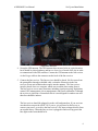
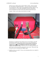
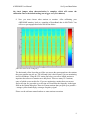
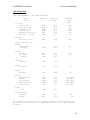
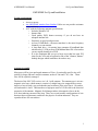
AWESOME User Manual
Set Up and Installation
AWESOME Set Up and Installation
System requirements
•
•
•
Access to power
An AWESOME monitor from Stanford. Often we can provide assistance
with installation.
A PC with the following minimal specifications:
o Includes Windows XP
o Internet link
o Good quality DVD burner necessary if you do not have an
adequate internet link
o Pentium 4 or equal speed processor
o At least 512MB Ram -- the more ram there is, the more frequency
channels you can monitor.
o A large hard drive - for storing large amounts of broadband data
when needed. 1.5GB per hour of broadband data fills it fast unless
you are rapidly burning it to DVD
o It is also important that you get a large tower that has open PCI
slots (for the A/D card) as opposed to one of the "slimmer, thinner"
desktop designs which sometimes do not have any.
Antenna Assembly
Most users will be given prelooped antennas of 2.6m. Occasionally specific sites will
qualify for larger and more sensitive antenna, such as 8.39m and 1.7m, 4.9m. These
sites will be explicitly arranged.
The basis of the 2005 VLF receiver is a 1 Ω, 1 mH, antenna. The antenna type is air core
magnetic wire loop, which means it consists of a single long wire wrapped one or more
times in a loop in such a way such that the total resistance of the wire loop is 1 Ω, and its
self-inductance is 1mH. This introduces a high pass cutoff of 159 Hz due to the electrical
properties of the antenna. Magnetic field changes induce electromotive forces in the
wire, thus inducing currents in the loop. There are several possible configurations of wire
that meet these requirements, and derive the physics of current induction. They are
reproduced here for convenience:
1
AWESOME User Manual
Set Up and Installation
Some Valid Antenna Configurations
Length
Square
AWG
Turns
Area
2
Weight
Wire
mV / pT (Input)
16.0 cm
20
47
256 cm
0.132 kg
30.1 m
1.20E-02
56.7 cm
18
21
0.3215 m2
0.331 kg
47.6 m
6.75E-02
0.831 kg
74.8 m
3.18E-01
2.09 kg
117.6 m
1.44E+00
0.838 kg
75.3 m
2.03E-01
1.70 m
4.90 m
2.60 m
16
14
16
11
6
12
2
2.89 m
2
24.01 m
2
1.69 m
2
Right
8.39 m
14
6
17.60 m
2.15 kg
121.5 m
1.06E+00
Isosceles
27.3 m
12
3
186.32 m2
Triangle
5.56 kg
197.7 m
5.59E+00
2
60.7 m
10
2
921.1 m
13.1 kg
293.1 m
1.84E+01
202 m
8
1
10201 m2
34.5 kg
487.7 m
1.02E+02
There are two shapes of antennae, square and isosceles triangle. The “length”
characteristic of the square shape refers to the length of a side. The “length”
characteristic of the right isosceles triangle corresponds to the length of the base (which is
along the ground). Because it is a right isosceles triangle, the triangle’s height is half that
of the base. The antenna thus makes a 45° angle at both corners on the ground, and a 90°
angle at the top (mast). The AWG column refers to “American wire gauge”, a measure
of the thickness of the wire used to wind the antenna. A lower AWG means a thicker
wire. Naturally, the larger antennae will need thicker wire in order to keep the resistance
below 1 Ω. The turns column refers to the number of times around the wire is wrapped,
and the last column shows the length of wire required for the antenna loop (of course,
you will need to leave some extra length on each side as well, to connect it to the
receiver).
Here is a complete parts list for the antenna and mast design pictured below:
Function
elevate antenna loops on mast
join sections of mast
fix cap screws to mast
attach guy wires and antenna to mast.
fix eyebolts to mast
attach guy wires to turnbuckle
tighten guy wires
quick clip guy wires to mast eyebolts
guy wires
crimp loops in guy wires
form loops at ends of guy wires
stake antenna loops and guy wires into gnd
Part Description
Aluminum poles - square 1.25" OD x 6ft.
Antenna wire loops
18-8 SS hex cap screw. 1/4" - 20 x 3"
18-8 SS Hex nylon insert lock nut
wire eyebolt 5/16"-18, 2" shank
18-8 SS hex nut 5/16" – 18
spring lock washer 5/16"
jaw 5/16" left hand thread
galvanized turnbuckle 5/16"
316SS spring snap
vinyl coated steel rope (2x20ft + 2x15 ft)
oval compression sleeves
light duty wire rope thimble
concrete form board stakes with holes
Qty
3
2
6
6
10
10
10
4
4
6
70ft
8
8
8
2
AWESOME User Manual
Set Up and Installation
The isosceles triangle antenna at WSO
The antenna should be oriented in a consistent, repeatable, and documented fashion, in
order for data from all different sites to be compared. We recommend orienting the
antenna in the following fashion: Align the NS antenna so that the loop is in the NS
plane, this can be either magnetic north or geographic north. You will need a compass or
a GPS device to align it properly, or some way to determine direction to within a few
degrees of accuracy. The other antenna should then be aligned along the EW direction,
and the orthogonality of the two antennae should be checked with a T-square.
To ensure that the polarity of the antennae is consistent from site to site, we recommend
orienting the +/- connections as follows: When you are standing to the north of the EW
antenna, looking south at it, if you follow the antenna loop from the + side to the – side,
the antenna loop should be clockwise. When you are standing to the east of the NS
antenna, looking west at it, following the + connection to the – connection should go
clockwise. Connect the antenna to the preamp using these configurations.
Building a Mast
Design of an apparatus to physically support the antenna loops should be based on the
specifics of the site – the weather, antenna size, ground condition, length of setup, etc.
3
AWESOME User Manual
Set Up and Installation
However, here is shown a sample design that has been used for the 8.39m2 triangular
base antenna. This design is fairly easy to set up, however it may not be so durable for
high winds or extreme weather conditions. As such, it is only recommended for sites that
will not see overly extreme conditions, or sites that will be monitored on a regular basis
by someone who can repair it if it breaks down.
The next page shows pictures of the antenna. The triangular antenna features a single
vertical mast, affixed to the ground via a wooden board that is bolted down. Four guide
wires (two attached just below the top of the mast, two about halfway up the mast),
stabilize the mast, and are staked into the ground so that guide wire is taut, but not too
tense. Finally, the four antenna loops are locked into place at the top of the mast,
stretched out, aligned to the proper directions, and then staked into the ground.
Once the antenna is successfully set up, the process of connecting the 2005 Stanford VLF
Receiver and readying it for acquisitions is as follows:
Setting up the monitor
1. To ensure that the polarity of the antennae is consistent from site to site, we
recommend orienting the +/- connections as follows: When you are standing to
the north of the EW antenna, looking south at it, if you follow the antenna loop
from the + side to the – side, the antenna loop should be clockwise. When you
are standing to the east of the NS antenna, looking west at it, following the +
connection to the – connection should go clockwise. Connect the antenna to the
preamp using these configurations.The preamp should be placed as close as
possible to the antenna but not directly under the path of one of the loops. The
photo below will show you proper placement.
E/W Antenna
N/S Antenna
Preamp
North
VLF Two Channel Orthogonal Magnetic Loop Antenna Configuration
4
AWESOME User Manual
Set Up and Installation
Preamplifier Connected to Antenna and Line Receiver
Open Preamplifier box
2. Install the NI-DAQ PCI card into an open slot in your computer. To do this you
must first open the cover to the computer tower and locate the open slots. Simply
insert the PCI card into an available slot gently but securely.
3. Insert the mother board and the filter card into the open slots in the line receiver.
Make sure they are in securely.
5
AWESOME User Manual
Set Up and Installation
Open Line Reciever
4. Set up the GPS antenna. The GPS antenna does not need to be in a quiet location,
but it should be placed outdoors and have a clear view of much of the sky in order
to communicate with GPS satellites. Connect the GPS antenna to the line receiver
via the N-type cable to the connector on the back of the line receiver.
5. Connect the line receiver. The line receiver should be placed 100 ft or more from
the preamplifier through a shielded cable, so that the electronics in the line
receiver do not emit radiation that couples into the antenna. The line receiver
must be placed close to a computer which can record the data coming from it.
The line receiver serves many functions, including signal processing, digitization
control, GPS management, power management, and system calibration. Although
the receiver is placed in a custom built box it is not designed for outdoor use and
therefore should be indoors.
The line receiver should be plugged in to the wall, and turned on. If you are in an
area that does not provide 60 Hz 110 V power, you will need to find a way to
convert your power, or to drive the line receiver’s DC input voltages directly from
an external source. When the line receiver is plugged in and receiving power the
blue light on the front should be lit.
6
AWESOME User Manual
Set Up and Installation
The line receiver connects to the computer with two cables – the first is a large
blue cable labeled “National Instruments”. This goes from the slot on the line
receiver labeled “PC ADC” to the corresponding slot on the back of the PC. The
second connection is a serial cable (null-modem) which goes from the line
receiver slot labeled “PC Serial” to the serial connector on the back of your
computer. Make sure all connectors and cables are on tight.
Outside of Line Receiver With all the Proper Connections
In general, it is a good idea to leave the line receiver on at all times, even when
not acquiring, and only turn it off only when you won’t be acquiring data for
many days in a row. It is important, however, that anytime you reboot the
computer for any reason, you should turn off the line receiver until the
computer has finished booting. If the line receiver is on when you boot up, you
may at times see the mouse arrow jumping all over the screen. If this occurs, turn
off your line receiver and reboot the computer again.
6. Install the software onto the PC. Please see the adjoining software user manual for
detailed instructions.
7
AWESOME User Manual
Set Up and Installation
7. Calibration
It is now time to calibrate your AWESOME monitor. Calibration will require the
use of a dummy loop. A dummy loop replicates the impedance of the intended
antenna, and enables signals to be injected at the input of the system. Throughout
the characterization process, the dummy loop (or an antenna) should be connected
to the preamplifier’s input, because system’s response (particularly at low
frequencies) can be properly estimated only when the VLF input is loaded with
the same impedance as it would with an antenna.
The process of calibration in the field requires executing a series of test
recordings and observations of the VLF receiver’s outputs. Within DAQSoftware
is a folder called “Calibration”. The folder contains a hierarchal tree of folders to
divide up the calibration tests by preamp cutoff setting, preamp gain setting, and
injected signal type. Initially, all acquisitions will be represented by an empty
text file, which act as a place holder until a MATLAB file for that particular test
is inserted. Namely, for each preamp frequency setting and gain setting, the
following tests should be run:
(1)
(2)
(3)
(4)
(5)
(6)
10mV signal injected into both channels
(a)
1 kHz
(b)
2 kHz
(c)
5 kHz
(d)
10 kHz
(e)
28 kHz
100mV signal injected into both channels
(a)
1 kHz
(b)
2 kHz
(c)
5 kHz
(d)
10 kHz
(e)
28 kHz
100mV, 10 kHz signal injected into only NS channel
100mV, 10 kHz signal injected into only EW channel
No signal into either channel
Sample VLF data
The fourteen different tests, for the four different gain settings, and the three different
cutoff sections, make a total of 168 different acquisitions needed. However, any gain
mode or frequency cutoff mode that is intended not to be used probably does not need to
be characterized.
During calibration, the jumper AuxA on the line receiver should be connected. This will
enable the automatic calibration tone to be triggered once every minute. Thus, all test
acquisitions for characterization need only be a minute long. It is important to remove
8
AWESOME User Manual
Set Up and Installation
the AuxA jumper when characterization is complete, which will restore the
calibration tone to the default setting (one trigger every five minutes)
8. Now you must choose what stations to monitor. After calibrating your
AWESOME monitor, look at a sampling of broadband data in MATLAB. You
will see a spectrograph that looks like the one below.
[does this need to be changed?]
The horizontal yellow lines that go all the way across the spectrograph are the stations
that your monitor can pick up. The left hand scale is the frequency you are monitoring
and is in Kilohertz. Using the VLF station list below you can see which stations to
input into the software to monitor on a daily basis. There are many VLF stations,
some of which are not on this list. If you are monitoring a station that you can not
find a call sign for, just make up a call sign or ID and enter the frequency in the input
field on the station dialog box. Enter in as many stations that you pick up as possible - stronger yellow bands imply a stronger frequency signal.
Please see the software manual on how to enter stations to monitor.
9
AWESOME User Manual
Set Up and Installation
VLF Station List
VERY LOW FREQUENCY (VLF) RADIO STATIONS
Station
Site
Station
ID
Frequency
(kHz)
Radiated
Power
(kW)
U.S. Navy
Cutler, ME
Jim Creek, WA
Lualualei, HI
LaMoure, ND
Aquada, Puerto Rico
Keflavik, Iceland
NAA
NLK
NPM
NLM
NAU
NRK
24.0
24.8
21.4
25.2
40.8
37.5
1000
250
566
500
100
100
Australia
Harold E. Holt,
NWC
19.8
1000
DHO
18.5
23.4
500
-
France
Rosnay
St. Assie
LeBlanc
HWU
FTA
HWU
15.1
16.8
18.3
400
23
-
Iceland
Keflavic
TFK
37.5
-
Federal Republic of
Germany
Rhauderfehn
Burlage
Italy
Tavolara
ICV
20.27
43
Norway
Noviken
JXN
16.4
45
Russia
Arkhanghelsk
Batumi
Kaliningrad
Matotchkinchar
Vladivostok
UGE
UVA
UGKZ
UFQE
UIK
19.7
14.6
30.3
18.1
15.0
TBB
26.7
150
100
100
100
100
input
input
input
input
input
Turkey
Bafa
United Kingdom
Anthorn
London
GQD
GYA
19.6
21.37
-
500
120
All information courtesy of Bill Hopkins, Technical Representative for
Pacific-Sierra Research Corp.. Updated by Michael Hill. Last updated:
02/22/05
10