Download Weather Forecast using Kalman Filter Algorithm with Warning

Weather Forecast using Kalman Filter Algorithm with
Warning System via GSM and Android Application
by
Trexia D. Capapas
Jezzelle Joyce Clarice M. Paule
Rochelle Lynn S. Vista
A Thesis Report Submitted to the School of EE-ECE-CoE
In Partial Fulfilment of the Requirements for the Degree
Bachelor of Science in Computer Engineering
Mapua Institute of Technology
March 2014
ii
ACKNOWLEDGEMENT
First and foremost, we would like to take this opportunity to express our deep sense of gratitude
to our advisor, Dr. Felicito S. Caluyo for his exemplary guidance, constant encouragement
throughout our thesis, for his patience and immense knowledge.
We would also like to thank Engr. Noel B. Linsangan, chairman of CpE course, for the intuitive
comments and guidance throughout the checking and editing of documentation.
We would also take this opportunity to thank the Accuweather company for providing online
forecasts which helps us to pursue and to complete this study especially on the testing part of the
system.
We would also like to thank our panels who have given us recommendations that are applicable
in the system. These insights are very useful and are used to improve our thesis.
Finally, we would like to thank our Almighty Father for giving us high hopes and being our
source of strength. To God be the glory.
iii
TABLE OF CONTENTS
TITLE PAGE
i
APPROVAL PAGE
ii
ACKNOWLEDGEMENT
iii
TABLE OF CONTENTS
iv
LIST OF TABLES
v
LIST OF FIGURES
vi
ABSTRACT
x
Chapter 1:
INTRODUCTION
1
Chapter 2:
REVIEW OF LITERATURE
6
Sensors
Weather Instruments
GSM
Weather Parameters
Predictive Algorithm
Kalman Filter
PIC16F877A Microcontroller
Summary
9
10
11
12
13
13
15
16
Chapter 3:
METHODOLOGY
17
Abstract
17
Introduction
17
Methodology
19
Design and Implementation of the Device
19
Applying Algorithm for the Prediction of Weather Conditions
24
Write a Program and Training of the System
29
Validating, Testing and Determining the Accuracy of the System
32
Results and Discussion
37
Determining the Accuracy of the Measurement of the Device
37
Temperature
37
Relative Humidity
38
Pressure
39
Determining the Accuracy of System Forecast to Accuweather Forecasts 41
iv
and Actual Measurements
Hourly Forecasts of Temperature
Hourly Forecasts of Relative Humidity
Hourly Forecasts of Pressure
Statistical Tool
Temperature – System Forecast and Actual Measurement
Relative Humidity – System Forecast and Actual Measurement
Pressure – System Forecast and Actual Measurement
Conclusion
References
41
43
47
50
50
51
53
55
57
Chapter 4: CONCLUSION
58
Chapter 5: RECOMMENDATIONS
60
REFERENCES
61
APPENDICES
62
v
LIST OF TABLES
Table 3.1: List of Components
20
Table 3.2: Tabulated data for Temperature
37
Table 3.3: Tabulated data for Relative Humidity
38
Table 3.4: Tabulated data for Pressure
39
Table 3.5: Comparison of Temperature Forecast between the System and
41
Accuweather
Table 3.6: Comparison of System Temperature Forecast to Actual Temperature
42
Measurement
Table 3.7: Comparison of Humidity Forecast between the System and
44
Accuweather
Table 3.8: Comparison of System Humidity Forecast to Actual Humidity
45
Measurement
Table 3.9 Comparison of Pressure Forecast between the System and Accuweather
47
Table 3.10 Comparison of System Pressure Forecast to Actual Pressure Measurement
48
Table 3.11 T-Test for Temperature
50
Table 3.12 T-Test for Relative Humidity
52
Table 3.13 T-Test for Pressure
53
vi
LIST OF FIGURES
Figure 1.1: Conceptual Framework
5
Figure 2.1: Weather Instruments
10
Figure 2.2: GSM/GPRS Module Framework
11
Figure 2.3: Circuit of the Kalman Filter
14
Figure 3.1: Block Diagram of the Device
20
Figure 3.2: Zigbee – Schematic Diagram
21
Figure 3.3: Temperature Sensor – Schematic Diagram
`
22
Figure 3.4: Pressure Sensor – Schematic Diagram
22
Figure 3.5: Humidity Sensor – Schematic Diagram
23
Figure 3.6: Schematic Diagram PIC16F877A Microcontroller
23
Figure 3.7: Process in Kalman Filter
25
Figure 3.8: Program Flowchart
31
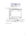
Figure 3.9: Selection of CSV file
35
Figure 3.10: Temperature – True Value vs. Measured Value
37
Figure 3.11: Relative Humidity – True Value vs. Measured Value
39
Figure 3.12: Pressure – True Value vs. Measured Value
40
Figure 3.13: Temperature
43
Figure 3.14: Relative Humidity
46
Figure 3.15: Pressure
49
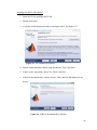
Figure 3.16: Driver Setup(x64)
62
Figure 3.17: MathWorks installer
63
Figure 3.18: File Installation Key Window
63
vii
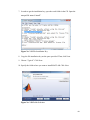
Figure 3.19: File Installation Key
64
Figure 3.20: Folder Selection
64
Figure 3.21: Installation Confirmation
65
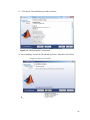
Figure 3.22: Installation Complete
65
Figure 3.23: Add a Bluetooth Device
66
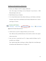
Figure 3.24: Kalaman.apk
67
Figure 3.25: Package Installer
67
Figure 3.26: Kalman Installation
68
Figure 3.27: Kalman GUI
69
Figure 3.28: Opening the Bluetooth Settings
69
Figure 3.29: Bluetooth Settings Window
70
Figure 3.30: COM Ports
70
Figure 3.31: Add COM Port
71
Figure 3.32: Standard Serial over Bluetooth
71
Figure 3.33: Modified COM Port
72
Figure 3.34: Zigbee Serial Connection
72
Figure 3.35: Complete Set-up of Zigbee
73
Figure 3.36: Device for Measuring Weather Parameters
73
Figure 3.37: Opening an Existing GUI File
74
Figure 3.38: .fig File
75
Figure 3.39: M-file
75
Figure 3.40: Run Button
76
Figure 3.41: Selecting Raw Data
76
viii
Figure 3.42: .fig File for Kalman Filter
77
Figure 3.43: Unhandled Internal Error
79
Figure 3.44: Error on Opening Serial Port
79
ix
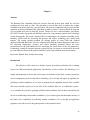
ABSTRACT
The Kalman Filter Algorithm filters the sensor's data and process data which are used for
predicting the next state or value. The algorithm is used in this study to predict the weather
condition on an hourly basis for a given location. The goal is to implement the processes and the
equations of the basic Kalman Filter Algorithm in order to produce a forecast based on the given
set of available data used to train the system. The device uses a microcontroller, specifically
PIC16F877A and is integrated with different sensors for each parameter and wireless technology
for the data transfer. The sensors include LM35 for temperature, the capacitive humidity kit for
humidity, MPX114AP for measuring the pressure and Zigbee technology for wireless data
transfer. The system includes methods for alerting people by using GSM and Android
application through Bluetooth. The tests conducted show that the sensors integrated in the device
for measuring temperature, pressure and relative humidity produced almost the same
measurements as the instruments used for measuring the actual value of the said parameters.
Furthermore, statistical tests show that the system forecast is accurate as evidenced by the small
per cent difference between the predicted and the actual values obtained from measurements.
Keywords: Kalman filter, weather forecasting
x
Chapter I
INTRODUCTION
The weather is basically a condition of the atmosphere at a certain time and place and is
measured by several parameters that contribute to it. Some of the weather parameters are
temperature, dry and wet bulb, amount of rainfall, dew point, humidity, pressure and wind. This
study will focus on forecasting a weather condition at a certain time in the future wherein a
warning system will be used to inform the people of incoming weather condition in the specific
area. Forecasting deals with the prediction of the upcoming weather condition and varies from
different time and location. Weather forecasts can be made using statistical dependencies, which
use predictor variables to extrapolate the weather situation, or simulations to gain information
about the possible state of the weather in the future. The prediction of weather conditions will be
based on the measurements gathered from the sensors of different parameters that affect weather.
The device containing the sensors will be placed in one location in the chosen locality.
Weather forecasting is considered as one of the objectives in a research dealing with the
atmosphere. K. Lerner and B. Lerner stated in the year 2003 that some methods used in
forecasting are: Climatology Method, Analog Method, and Numerical Weather Prediction
(NWP). The Climatology Method is a simple way of forecasting and involves average statistics
that are gathered in many years. The Analog Method is a forecasting method that is more
complicated compared to the Climatology Method. This method basically examines the present
forecast and compares it to the past forecasts which actually look familiar or form an analogy.
Basically, the forecaster would assume that the forecast would behave in the same as the weather
did in the past. On the other hand, Numerical Weather Prediction (NWP) is an algorithm the that
uses a computer for forecasting. Forecast models run on supercomputers which show the
1
prediction on weather parameters such as temperature, humidity, pressure, rainfall and wind. The
features predicted by the supercomputers which interact with each other are examined by the
forecaster and used to produce the present weather.
There are some downsides in the existing prediction method. The said method is only
effective when most of the data gathered are the same with the expected data in a specific time of
the year. Thus, if the values were different at that time, climatology method will not succeed,
which will result in a difference between the previous and current time. In addition, NWP’s
equation in predicting certain parameters leads to a low precision and low accuracy, especially
when the previous data are completely unknown. From the dissertation of Hester Gerbrecht Marx
in 2008, "Forecasts generated by Numerical Weather Prediction (NWP) models are imperfect
due to errors in the initial and boundary conditions that are fed into the model. Therefore, there is
a need to apply statistical post-processing techniques in modeled forecast fields to improve
forecast quality and value‖.
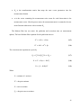
The objective of this study is to design a system for weather prediction with a warning
system via GSM and Android Application.. Specifically, it aims to achieve the following: (i) to
design and implement a device that will measure and monitor actual basic weather parameters
such as temperature, pressure and relative humidity, (ii) to develop and apply an algorithm for
predicting weather conditions, (iii) to write a program for the algorithm and use 80% available
data sets to train the system, (iv) to use 20% of the available data sets to validate the system,
(v) to simulate the system by applying available initial conditions such as those provided by the
device for monitoring actual weather conditions, (vi) to test the system and determine in terms of
the limits of its capabilities in predicting weather conditions, (vii) to develop an application
program to provide access by the general public to the predicted values.
2
This study will be significant in informing an individual or group of people with the
information on the anticipated weather over forthcoming one to three days for sites in the areas
so that they may take necessary precautions from a coming danger in the chosen locality. Thus,
in these cases, forecasts are one of the main aspects that may help save lives or prevent damage,
which could be avoided by preventive arrangements. The warning will be based on the predicted
weather due to different parameters at a specific date or time. Furthermore, the device will use an
algorithm in predicting the weather by analyzing vital parameters such as probabilities of
temperature, atmospheric pressure, and relative humidity. Data regarding weather conditions on
a specific locality from PAGASA will be monitored in order to produce accurate and valid
weather forecast.
Since the weather is continuous, multidimensional, dynamic and chaotic, and hence
difficult to predict, the results will not be very accurate. Due to these circumstances, weather is
observed to be changing simultaneously, which leads to a conclusion that forecast can be out of
date easily. Hence, the algorithm will determine the limits of the predicted weather condition
rather than its accuracy. Moreover, Quezon City will be the chosen locality wherein data
measured by the sensors located in the said locality will be processed using an algorithm that is
not being used by PAGASA such as the Kalman filter. The wireless device would basically send
the data measured using the sensors into the data logger. After that, measured parameters will be
used in the application of the algorithm for prediction purpose. Using the algorithm, parameters
used by PAGASA can also be predicted. These include rainfall, maximum and minimum
temperature, dew point, vapor pressure, relative humidity, mean sea level pressure, prevailing
winds and cloud. Selected parameters such as temperature, atmospheric pressure and relative
humidity will utilize the historical data and sensor data for prediction in the application of the
3
algorithm. Developing an application program to provide access by the general public to the
predicted values will be limited only in sending text messages to selected people such as the
barangay officials and through an Android Application using Bluetooth.
4
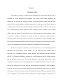
CONCEPTUAL FRAMEWORK
Figure No. 1.1 Conceptual Framework
5
Chapter 2
REVIEW OF RELATED LITERATURE
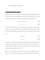
Statistical post-processing techniques are used to remove the systematic bias in modelled
data (Marxs, H.G., 2008). There are actually common features that characterize several methods
for weather prediction. The said features are sensors data acquisition, assimilation, processing of
received data and post-processing the result, and finally, representing the obtained results and
forecasts.
In sensors data acquisition, there are specialized sensors and sensor modules in collecting
data for typical meteorological parameters of the atmosphere. It has been said that processing
received data is made with the help of a previously created mathematical model of a combination
of thermodynamic equations which describe the state of the atmosphere in a given location in
any moment of time, and analysis of numerical statistical data (I. Simeonov, H. Killifarev and R.
Ilarionov, 2006).
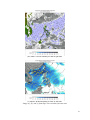
From the Daily Weather Forecast of Kidlat Pagasa, in the Philippines, the following
weather parameters have interest to the users of the forecast, cloudiness, rainfall and wind.
Basically, weather maps such as surface maps and upper-air maps, are used by weather
forecasters since they depict the distribution patterns of temperature, pressure, humidity and
wind at different levels of the atmosphere. Furthermore, there are five standard levels of the
upper-air maps that are constructed twice daily at twelve-hourly interval. The surface maps are
made four times daily at six-hourly intervals. On the surface maps, the distribution patterns of
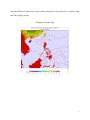
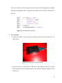
rain or other forms of precipitation and cloudiness can also be delineated. The figures below
6
show the different weather maps: (a) the surface temperature, (b) cloud cover, (c) surface wind
and, the (d) upper air map.
Philippines Weather Map
(a) Surface Temperature on Saturday 02 Mar at 2pm PHT
7
(b) Cloud Cover on Saturday 02 Mar at 8pm PHT
(c) Surface Wind on Sunday 03 Mar at 2am PHT
Image (a), (b), and (c) from http://www.weather-forecast.com/
8
(d) Upper air map of Southeast asia
Image from http://weather.uwyo.edu/upperair/uamap.html
2.1 Sensors
From an article, ―What forces affect our weather?‖ in Annenberg Learner and
Foundation, 2013; it has been stated that devices are required in order to view large weather
system specifically on a worldwide scale. From this point, satellites are considered as invaluable
which shows large weather events and other global weather systems. For every satellite, two
types of sensors were used such as the imager and the sender which is a visible light sensor and
an infrared sensor that reads temperature, respectively.
9
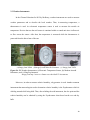
2.2 Weather Instruments
In the Climate Education for K12 by McKemy, weather instruments are used to measure
weather parameters and to describe the local weather. Thus, in measuring temperature, a
thermometer is used. An electronic temperature sensor is used to measure the outside air
temperature. Devices that use the said sensor is contained within a vented unit since it allows air
to flow across the sensor. After that, the temperature is measured while the thermometer is
protected from the direct heat of the sun.
(a)Image from NOAA (b)Image from Wikimedia Commons (c) Image from NASA
Figure No. 2.1 Weather Instruments (a) Electronic Temperature Sensor, (b) Modern Aneroid
Barometer, and (c) Sling Psychrometer
Image from http://www.nc-climate.ncsu.edu/edu/k12/.instruments
Moreover, in order to measure relative humidity, a hygrometer is used. Another common
instrument that meteorologists used to determine relative humidity is the Psychrometer which is
whirling around while being held. Thus, after whirling the said instrument, the dew point and the
relative humidity can be obtained by using the Psychrometer chart based on the wet and dry
bulb.
10
For atmospheric pressure, barometers are used in order to measure the said parameter.
One of the most common types of barometer is an aneroid barometer which uses a sealed can of
air to detect changes in atmospheric pressure. The concept of using this instrument is that as the
atmospheric pressure goes up, it pushes in on the can, and the can is slightly reduced in volume,
moving an indicator needle towards higher pressure. If the atmospheric pressure goes down, the
can expands slightly and the needle indicates lower pressure. Nowadays, the electronic signal
containing the trends of the pressure is reported for a computer which is then plotted in a
computer monitor instead of using special graph paper in tracking the change in pressure.
2.3 GSM
Suriya Shopna stated that GSM, which stands for Global System for Mobile
Communications, is developed by the European Telecommunications Standards Institute (ETSI).
It is also a set which is usually used to describe the protocols used by mobile phones for the
second generation digital cellular networks. Also, it was developed in order to replace first
generation (1G) analog cellular networks (2013).
Figure No. 2.2 GSM/GPRS Module Framework
Image from http://www.engineersgarage.com/articles/gsm-gprs-modules
GSM can be connected to control panels to provide the following facilities: report
system events via text messaging to mobile telephones, remotely arm, disarm and obtain the
11
current status of the alarm system via text messaging, high-speed modem communication for
upload/download and backup signalling path for digital communicator (Telexecom).
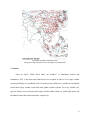
2.4 Weather Parameters
The PAGASA deals with the measurement of almost fifteen (15) weather parameters.
Weather parameters are determined directly by human observation, by instruments, or by a
combination of both. These parameters are shown below.
PAGASA described the parameters as follows: maximum temperature is the maximum
temperature in °C recorded for the day, which occurs in the early afternoon while the minimum
temperature is the minimum temperature in °C recorded for the day, usually occurring during the
early hours of the morning (before sunrise). To compute for the mean temperature, get the
average of the maximum and minimum temperature. The dry bulb temperature gave the air
temperature in °C at the time of observation and the wet bulb temperature gives the temperature
in °C that an air parcel would have if cooled to saturation at constant pressure by evaporating
water in it. The dew point temperature is the temperature in °C at a given pressure, wherein the
air must cool down for it to saturate. Also, this parameter is the temperature when the moisture
begins to condense causing the formation of dew on objects.
12
Relative humidity is the ratio of the amount of water vapor actually in the air to the
maximum amount the air can hold at that temperature (Schlatter T.,2010). Vapor pressure must
also be included that denotes the partial pressure of water vapor in the atmosphere. As the water
evaporates, additional water vapor is introduced into the space above and pressure increases
slightly as the new vapor is added. The increasing pressure is due to an increase in the partial
pressure of water vapor. Mean Sea Level Pressure or MSLP is also considered the atmospheric
pressure at mean sea level and is the force which is exerted per unit area at the mean sea level
through the weight of the atmosphere.
The rainfall describes the amount of precipitation and is usually expressed in millimeters.
The cloud can also be a weather variable that depicts the amount of cloud present in the sky,
expressed in oktas of the sky cover. Prevailing wind direction is most frequently observed during
a given period while the average wind speed in meters per second is the arithmetic average of the
observed wind speed.
2.5 Predictive Algorithm
Kalman Filter
Theoretically, the Kalman filter is an estimator for what is called the linear-quadratic
problem, which is the problem of estimating the instantaneous ―state‖ a linear dynamic system
perturbed by white noise—by using measurements linearly related to the state but corrupted by
white noise. The resulting estimator is statistically optimal with respect to any quadratic function
of estimation error (M. Grewal and A.P Andrews, 2008).
13
Thus, according to K. Sreedhar, A. Venu, and A. Hriprasad, the Kalman Filter consists
of two steps: the prediction and the correction. This procedure is repeated for each time step with
the state of the previous time step as initial value. Therefore, the Kalman Filter is called as a
recursive filter (2013).
Figure No. 2.3 Circuit of the Kalman Filter
Kleinbauer stated in 2004 that the basic components of the Kalman Filter are the state
vector, the dynamic model and the observation model. State vector contains the variables of
interest. It describes the state of the dynamic system and represents its degrees of freedom. The
variables in the state vector cannot be measured directly, but they can be inferred from the values
that are measurable (Subash, J.,2012). The state vector has two values, such as the priori value xwhich represents the predicted value before the update, and the posteriori value + which is the
corrected value after the update.
It is said that the significant advantages of Kalman filter are that it combines measured
data as well as previous knowledge about the system and measuring devices to produce an
14
optimal estimate of the desired variables. Also, compared to other filters, it minimizes the error
significantly (Vij V. and Mehra R.,2011) s.
However, Graham Hesketh stated that Kalman Filter is computationally complex,
especially for large numbers of sensor channels, it requires conditional independence of the
measurement errors (sample-to-sample). It also requires linear models for state dynamics and
observation processes, and getting a suitable value for Q (a.k.a. tuning) can be something of a
black art (2000).
2.6 PIC16F877A Microcontroller
In the study of Ibrahim Al-Adwan and Munaf S. N. Al-D entitled "The Use of ZigBee
Wireless Network for Monitoring and Controlling Greenhouse Climate", they used PIC16F877A
microcontroller for the purpose of storing the instantaneous values of the environmental
parameters they focused on and the Zigbee for wireless communication. The environmental
parameters include the temperature, humidity and light or solar radiation. According to them,
"sensors provide input information for the automation system by measuring the climate variables
of the greenhouse. Sensor-generated signals are acquired and conditioned by a PIC16F877A
microcontroller. These sensors are connected to a PIC16F877A microcontroller which consists
of embedded ADCs." They also used a ZigBee transceiver which is directly connected to the
microcontroller to provide a wireless connection with the central station.
From the study, ―A Low-Cost Microcontroller-based Weather Monitoring System‖ of
Kamarul Noordin, Chow Onn and Mohamad Isamail, they measure temperature, atmospheric
pressure and relative humidity remotely by using the appropriate sensors that are not only
important in environmental or weather monitoring but also crucial for many industrial processes.
15
The analogue outputs of the sensors are connected to a microcontroller specifically PIC16F877A
through an ADC for digital signal conversion and data logging.
2.7 Summary
According to the research paper entitled, ―Correcting Temperature and Humidity
Forecasts using Kalman Filtering: Potential for Agricultural Protection in Northern Greece‖ of
Manolis Anadranistakis, Kostas Lagouvardos, Vassilik Kotroni and Helias Elefteriadis, the
application of the Kalman theory, filtering can substantially reduce errors of the near-surface
temperature and humidity forecasts provided for 2-3 days ahead in time. Based on the corrected
forecasts, farmers can then schedule their fungicide spraying programs according to the expected
weather, thus reducing the cost and the ecological impact of frequent preventive spraying
interventions. Also, the success of the method is also supported by the fact that after correction
and for both parameters, the mean error decreases to values close to zero, showing that the
method is able to provide almost unbiased corrected forecasts, while the standard deviation of
the error also decreases by 50%.
Similar to the researchers’ proposed device, it mainly focused on forecasting weather
parameters such as temperature and humidity using Kalman Filter Algorithm. An additional
weather parameter, pressure, is also being measured by the device. The work of Manolis
Anadranistakis, Kostas Lagouvardos, Vassilik Kotroni and Helias Elefteriadis has been
motivated by the importance of meteorological conditions for the protection of potato cultivation
from mildew. On the other hand, the proposed device has a warning system to inform the people
of the possible damage that the forthcoming weather might bring. GSM for emergency text and
an Android Application are used as a warning system for easy transmission of data.
16
Chapter 3
Abstract
The Kalman Filter Algorithm filters the sensor's data and process data which are used for
predicting the next state or value. The algorithm is used in this study to predict the weather
condition on an hourly basis for a given location. The goal is to implement the processes and the
equations of the basic Kalman Filter Algorithm in order to produce a forecast based on the given
set of available data used to train the system. The device uses a microcontroller, specifically
PIC16F877A and is integrated with different sensors for each parameter and wireless technology
for the data transfer. The sensors include LM35 for temperature, the capacitive humidity kit for
humidity, MPX114AP for measuring the pressure and Zigbee technology for wireless data
transfer. The system includes methods for alerting people by using GSM and Android
application through Bluetooth. The tests conducted show that the sensors integrated in the device
for measuring temperature, pressure and relative humidity produced almost the same
measurements as the instruments used for measuring the actual value of the said parameters.
Furthermore, statistical tests show that the system forecast is accurate as evidenced by the small
per cent difference between the predicted and the actual values obtained from measurements.
Keywords: Kalman filter, weather forecasting
Introduction
The objective of this study is to design a system for weather prediction with a warning
system via GSM and Android Application.. Specifically, it aims to achieve the following: (i) to
design and implement a device that will measure and monitor actual basic weather parameters
such as temperature, pressure and relative humidity, (ii) to develop and apply an algorithm for
predicting weather conditions, (iii) to write a program for the algorithm and use 80% available
data sets to train the system, (iv) to use 20% of the available data sets to validate the system,
(v) to simulate the system by applying available initial conditions such as those provided by the
device for monitoring actual weather conditions, (vi) to test the system and determine in terms of
the limits of its capabilities in predicting weather conditions, (vii) to develop an application
program to provide access by the general public to the predicted values.
17
This study will be significant in informing an individual or group of people with the
information on the anticipated weather over forthcoming one to three days for sites in the areas
so that they may take necessary precautions from a coming danger in the chosen locality. Thus,
in these cases, forecasts are one of the main aspects that may help save lives or prevent damage,
which could be avoided by preventive arrangements. The warning will be based on the predicted
weather due to different parameters at a specific date or time. Furthermore, the device will use an
algorithm in predicting the weather by analyzing vital parameters such as probabilities of
temperature, atmospheric pressure, and relative humidity. Data regarding weather conditions on
a specific locality from PAGASA will be monitored in order to produce accurate and valid
weather forecast.
Since the weather is continuous, multidimensional, dynamic and chaotic, and hence
difficult to predict, the results will not be very accurate. Due to these circumstances, weather is
observed to be changing simultaneously, which leads to a conclusion that forecast can be out of
date easily. Hence, the algorithm will determine the limits of the predicted weather condition
rather than its accuracy. Moreover, Quezon City will be the chosen locality wherein data
measured by the sensors located in the said locality will be processed using an algorithm that is
not being used by PAGASA such as the Kalman filter. The wireless device would basically send
the data measured using the sensors into the data logger. After that, measured parameters will be
used in the application of the algorithm for prediction purpose. Using the algorithm, parameters
used by PAGASA can also be predicted. These include rainfall, maximum and minimum
temperature, dew point, vapor pressure, relative humidity, mean sea level pressure, prevailing
winds and cloud. Selected parameters such as temperature, atmospheric pressure and relative
humidity will utilize the historical data and sensor data for prediction in the application of the
18
algorithm. Developing an application program to provide access by the general public to the
predicted values will be limited only in sending text messages to selected people such as the
barangay officials and through an Android Application using Bluetooth.
This chapter discusses the methods that are used to gather, analyze, interpret and report
data. It defines the scope and limitations of the research design used. Furthermore, this chapter is
divided into three sections. The first section includes the data gathering to be performed which
discussed the processes used to come up with the data. The next section is about the processes
performed and analysis of the collected data and lastly, the validation of the results.
Methodology
3.1 Design and Implementation of the Device
The basic weather parameters such as temperature, atmospheric pressure and relative
humidity will be measured using a device designed to gather these parameters. It uses specific
sensors for each parameter to collect data. The sensors will be integrated into one device to have
the capability to measure these three basic weather parameters approximately every 10 seconds
for the real time purposes. The measurements from the sensors will then be sent wirelessly using
Zigbee technology. The data logger will be implemented using MATLAB to read, collect and
gather data that will be received from the sensors. The data logger will display 10 samples of
measurement from each parameter.
19
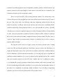
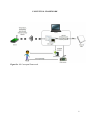
Figure No. 3.1 Block Diagram of the Device
The block diagram of the device is shown in Figure3.1. Sensors for each parameter and
the Zigbee module for wireless data transfer were connected in the microcontroller. The specific
sensors and components listed in Table 3.1 are used to design and implement the device. The
sensors used were affordable and light in size, thus, making the device cheap and handy.
Table No. 3.1 List of Components
Component
PIC 16F877A
Temperature Sensor (LM35)
Humidity Sensor (Capacitive Humidity Kit)
Atmospheric Pressure Sensor (MPX114AP)
GSM Module
As shown in Figure3.1, the PIC16F877A microcontroller was used to connect the three
sensors and the standard Zigbee for the wireless data transfer. This microcontroller was used
because it has an advantage over other microcontrollers which is easy to use attributable to its
large number of peripherals which was approximately 40 pins. For the humidity sensor, a
capacitive humidity sensor kit was used. Taranovich stated in 2011 that a capacitive humidity
sensor is more appropriate to use than a resistive humidity sensor kit because the capacitive kit
20
ranges its percent relative humidity from 0 to 100 while in a resistive sensor kit; it only ranges
from 20 to 90 percent only.
The schematic diagram for the Zigbee connection is shown in Figure3.2. It has been said
that ZigBee is more advantageous to use than other wireless technologies because it requires low
consumption of power and low data rates (Scheneider Electric Industries SAS, 2011). Basically,
two Zigbee modules were used in the design wherein one will serve as the transmitter and the
other will serve as the receiver. The transmitter is used to transfer data coming from the sensors
into the data logger which is implemented in MATLAB. The receiver is used to read the data
coming from the microcontroller which are parameter measurements.
Figure No. 3.2. Zigbee – Schematic Diagram
For the temperature sensor, LM35 is used, which is depicted in the schematic diagram
shown in Figure3.3. In this study, PIC16F877A is used as the microcontroller which has 8
channels (A0-A5 and E0-E2) of 10 bit resolution ADC (analog-to-digital converter) module
(Microchip,2012). Since the input voltage is 5V which is the maximum value, the range of
voltages starting at 0V and ended by 5V needs to be separated into equal steps starting from 000
up to 1023.
21
Figure No. 3.3 Temperature Sensor – Schematic Diagram
The ADC step can be calculated using equation 3.1:
(3.1)
Solving for the ADC step, a value of 4.883 mV is calculated wherein it is the minimum voltage
that the ADC can read. To change or convert the ADC reading to Celsius degrees, the input
voltage is divided by 10mV/C which is the sensor's sensitivity. Thus,the equation used is shown
below:
(3.2)
Figure 3.4 shows the schematic diagram for the pressure sensor. In addition to the sensing
element, a capacitor of 0.1 F is connected. Connecting a capacitor to the ground will filter
unwanted frequencies from the input voltage.
Figure No. 3.4. Pressure Sensor – Schematic Diagram
22
As observed in the schematic diagram of humidity sensor in Figure3.5, a 22KΩ resistor
is connected to the sensor element. This sensor will produce an analog voltage which will go into
an analog-to-digital converter or ADC of the microcontroller. Then, it will generate a digital
voltage output for humidity. Almost same process will be performed on the other sensors:
temperature sensor and pressure sensor.
Figure No. 3.5. Humidity Sensor – Schematic Diagram
Figure No. 3.6. Schematic Diagram of PIC16F877A Microcontroller
Figure3.6 shows the schematic diagram for the PIC16F877A microcontroller. As
illustrated in the previous schematic diagrams, the temperature, pressure and relative humidity
sensors are directly connected to the RA0, RA1, and RC5 pin of the PIC16F877A
23
microcontroller respectively. The transmitter Zigbee and receiver Zigbee are connected to pin 25
and pin 24 of the microcontroller, respectively. A crystal oscillator is connected to PIC16F877A
microcontroller because it has no internal oscillator which is one of its disadvantages.
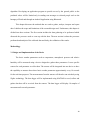
3.2 Applying the Algorithm for the Prediction of Weather Conditions
Kalman Filter is commonly referred as an optimal recursive computation of the leastsquares algorithm. It is a subset of a Bayes Filter where the premise of a Gaussian distribution
and that the current state is linearly dependent upon the previous state are imposed (Dhar S.,
et.al, 2010). It is optimized in a way that the Kalman filter minimizes the mean square error of
the estimated parameters of all noise that is Gaussian (Mastro, 2013).
In this study, the Kalman filter algorithm equations will be applied by using a simple onedimensional signal. The information that will be used in this study are accessible from the
historical data based on the last known measurements of temperature, relative humidity, and
pressure and current reading of measurements of the three parameters in the area. The data from
the two sources such as current measurements and historical data, are combined and processed
together to make the best possible estimate of the temperature, relative humidity, and pressure.
The Kalman Filter algorithm converges the estimation of a value into correct estimations.
Thus, assuming a poor estimated Gaussian noise parameter present in a signal will be corrected.
"The better you estimate the noise parameters, the better estimates you get" (Esme B., 2009).
Figure3.7 shows the step by step process in Kalman Filter which will be discussed further in the
various steps in dealing with Kalman Filter.
24
Basic Linear Kalman Filter
Figure No. 3.7 Process in Kalman Filter
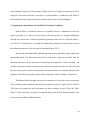
Ramsey Faragher stated in 2012 that there are two models associated with the Kalman
filter. Equations 3.3 to 3.9 and the corresponding function or significance are presented in the
25
said IEEE magazine. The Kalman filter model assumes that the state of the system during time
evolved at time −1 because of the prior state which is expressed in equation 3.3.
(3.3)
where

is the state vector containing the terms of interest for the system (temperature, relative
humidity and pressure) at time .

is the vector containing any control inputs

is the state transition matrix which applies the effect of each system state parameter at
time

is the control input matrix which applies the effect of each control input parameter in
the vector

on the system state at time
on the state vector
is the vector containing the process noise terms for each parameter in the state vector.
The process noise is assumed to be drawn from a zero mean multivariate normal
distribution with covariance given by the covariance matrix
The measurements of the system can be performed by using the equation (3.4) which
represents the second model
(3.4)
where

is the vector of measurements
26

is the transformation matrix that maps the state vector parameters into the
measurement domain

is the vector containing the measurement noise terms for each observation in the
measurement vector. Like the process noise, the measurement noise is assumed to be zero
mean Gaussian white noise with covariance
.
The Kalman filter has two states: the prediction and correction state (or measurement
update). The basic Kalman filter equations for the prediction state are
̂
̂
(3.5)
(3.6)
The correction state equations are given by
(3.7)
̂
̂
̂
(3.8)
(3.9)
Where
̂ = estimate of
at time
̂ = the prior estimate
= error covariance
= the prior error covariance
27
= Kalman gain (Ramsey Faragher,2012)
Steps in using the Kalman Filter Algorithm
Step 0: Build the model. The derivations will consider a simple one-dimensional signal. Thus,
the entities in the model are represented in numerical value and not in matrix form. The original
equation is shown in equation (3.3) and the reduced equation is given in equation (3.10).
(3.3)
(3.10)
The value of
is equated to a value of 1 since the next value will be the same as the previous
one due to its recursive part which is the nature of Kalman filter. Then, the
parameter equates
to a value of 0 and eliminated from the equation since no control signal was involved in this
study.
(3.4)
(3.11)
The equation (3.4) shows the linear combination of the measurement value and the signal value.
This equation is then brought down to simpler equation which is shown in equation (3.11) by
having the parameter H equated to a value of 1 because in real life, state value and some noise
are present in measurable value (Esme B., 2009).
Step 1: Set t = 0, then select the initial guess for
and
. The variable
and
. For the initial guess, let
does notequated to a value of 0 because this would mean that there
28
is no noise in the environment which is not true and impractical. Letting
would lead all
the consequent ̂ to be zero.
Step 2: Compute the Kalman Filter estimate and covariance:
A. Compute the Kalman Gain
(3.12)
B. Compute the estimate
̂
̂
̂
(3.13)
C. Compute the estimate covariance
(3.14)
Step 3: Update
Step 4: Set value for the evolution model prior estimate ̂ and prior error covariance
and
repeat step 2
A. Set ̂
̂
B. Set
(3.15)
(3.16)
3.3 Write a program and train the system
Write a program for the Algorithm
The program for weather prediction using Kalman Filter is implemented in MATLAB. It
is a high-level language and interactive environment for numerical computation, visualization,
29
and programming. The MATLAB allows analysis of data, developing algorithms and creating
models and applications (The MathWorks Inc., 2013). The step by step procedures in dealing
with Kalman Filter that were discussed earlier are implemented in MATLAB. The program
flowchart implemented for the system is presented in Figure 3.8.
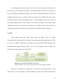
Training of the System
Accuweather is a company that produces forecasts for places everywhere in the US and
other locations worldwide including the Philippines. Thus, Accuweather is considered as the
World's Weather Authority. In this study, the historical data needed to train the system are
obtained from the Accuweather site. 80% of the available data is used to train the system while
the remaining 20% data is used to validate the system. The gathering of data is based on the short
range (hourly forecast) which will be used in testing the system. For the short range, the
gathering of data was based on an hourly forecast of the Accuweather for Quezon City which
was the target location for the testing of the system.
The collected data include only the parameters used in this study such as the temperature,
pressure and, relative humidity. The data will be arranged in order by time and tabulated in a
CSV file, then saved in the folder where the Kalman Filter.Fig and m file are located. In
executing the program, MATLAB is used which contains the processes and equations of Kalman
Filter, the program will first ask for a CSV file. After selecting the specific CSV file, the system
will then calculate for the parameters such as the prior estimate, prior error covariance, Kalman
gain, estimate, and estimate covariance which will be essential in forecasting the next state of
weather condition.
30
Software Development
START
Click Start Data
Acquisition
Select .csv
file
Process the
Historical Data
Receive measurements
for temperature,
humidity and, pressure
Tabulate and plot
the estimated
measurement
Send
Warning
Text?
Sends a command to
PIC16F877A
microcontroller for
GSM
No
No
Yes
Yes
Continue
Monitoring
?
No
Click Stop Data
Acquisition
Figure No. 3.8 Program Flowchart
END
31
3.4 Validating, Testing and Determining the Accuracy of the System
The validation of the device ensured that the system meets the requirements and
specifications stated in Chapter 1. It includes the following parts: (1) the device can measure and
monitor the actual basic weather parameters and (2) the prediction of the three weather
parameters (temperature, pressure and relative humidity) using the Kalman Filter algorithm. A
test will be conducted in each part to validate the method.
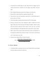
3.4.1 Procedures to be followed in measuring the accuracy of measurements of the
device
The test required only the data logger part of the program which is responsible for gathering,
monitoring, and displaying the measurements received by the laptop from the sensors
integrated in the device. Each parameter was subjected to a scenario wherein two types of
measurements were acquired: true value using the right instrument for measuring a certain
weather parameter and measured value using the measurements of the device displayed in the
data logger. Instruments used in the test for measuring the true value are the digital
thermometer for the temperature, electronic barometer for pressure and the Accuweather site
for the relative humidity. The differences between the measured value to the true value were
expressed by the calculating percent difference.
3.4.1.1 Temperature
The steps in the procedure for temperature measurements are listed below,
32
1. Set up the devices and the laptop in a room. Plug in the device (bigger one) and
connect the other device (smaller one) in the laptop using USB to serial port
cable.
2. Place the digital thermometer and the device (bigger one) within a box.
3. Run the M-file of the Kalman Filter algorithm using MATLAB.
4. Using a blower, heat up the temperature inside the box. Set the measurement of
the true value to 43°Celsius.
5. Click the Start Data Acquisition button found in the GUI of the program.
6. Record the measured value of the temperature which is exhibited in the data
logger of the system. Since the program will output 10 samples, compute its mean
and record under the Measured Value column. At the same time, record the
measurement displayed in the digital thermometer under the True Value column.
7. Make 10 trials of the test and record the collected data. In the succeeding trials, let
the temperature inside the box cool down. Set the 10th trial to have a measurement
of 29° Celsius for the True Value.
8. Compute the percentage difference using the equation
%PD =
|
|
3.4.1.2 Relative Humidity
1. A similar procedure as in the previous test is used to install the devices and laptop
in this test which was taken in Las Pinas City.
33
2. Visit the website of Accuweather or go to the link below and select the Las Pinas
link button. Click the Hourly Forecast link button on the left side of the window.
http://www.accuweather.com/en/ph/philippines-weather
3. In the Accuweather site, the forecast measurements of relative humidity per hour
are displayed. Record 10 measurement samples and its corresponding time for the
true value, which will be used as the reference for conducting the measurement
using the device.
4. Compute the percentage difference of the measured value to the true value using
the equation used in the previous test.
3.4.1.3 Pressure
1. The trial was conducted in Mapua Institute of Technology wherein the device was
positioned on each floor after each trial from higher to lower altitude.
2. For every step, record the change of value in pressure which is reflected in the
data logger. This data will be recorded under measured value. In assessing the
true value of pressure, an electronic barometer was applied.
3. Calculate the percentage difference of the measured value to the true value using
the equation used in the previous test.
3.4.2 Procedures to be followed in examining the system for the prediction of the three
weather parameters using a Kalman Filter algorithm
1. To begin, install the two devices and the laptop. Plug the device (bigger one) and plug
the other device (smaller one) into the laptop using USB to serial port cable.
2. Run the M-file of the Kalman Filter program using a MATLAB software.
34
Note: The version of MATLAB to be used in executing the M-file must support the
table property.
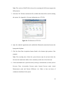
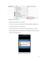
3. Select the CSV file that contains the 80% available data that will be used for training
the system. See Appendix A for more information on a CSV file.
Figure No. 3.9 Selection of CSV file
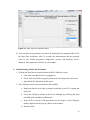
4. Open the Android Application and establish the Bluetooth connection between the
laptop and cell phone.
5. Click the Start Data Acquisition button found in the bottom right portion of the
program.
Note: The recording time of data for system forecast must be an hour before the
forecast time stated in the table to have consistency in the time of two forecasts.
6. Collect and tabulate the system forecast by having a column name (in order) such as
Forecast, Time, Accuweather Forecast (unit), System Forecast (unit), Actual
Measurement (unit) and Percent Difference (%). Make at least ten hours of
continuous simulation of the system.
35
Note: The collection of measurements for the two forecasts (system forecast and
Accuweather forecast) must be every hour and the actual measurement is collected in
the Accuweather site by clicking the Now tab in the same window for Hourly
Forecasts during the time stated in the forecast time.
7. Plot the system and Accuweather forecast and actual measurements to visually
represent the results of the three sets of parameters.
8. Compute the percentage difference to determine the accuracy of system forecast to
the Accuweather forecast and system forecast to actual measurements.
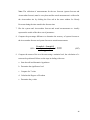
%PD =
|
|
(3.17)
9. Compare the means of the two forecasts using a statistical tool, the calculation of ttest must be performed. Below are the steps in dealing with t-test:
a. State the null and alternative hypotheses
b. Determine the significance level
c. Compute for T value
d. Calculate the Degrees of Freedom
e. Determine the p-value
36
Results and Discussion
3.4.1 Determining the Accuracy of the Measurement of the Device
Temperature:
Table No. 3.2 Tabulated Data for Temperature
TRIAL
1
2
3
4
5
6
7
8
9
10
Measured Value
(°C)
43.4320
42.8421
40.5400
37.8000
36.1126
34.6480
33.1840
32.6960
31.7290
29.2800
True Value
(°C)
43.5
42.7
40.5
38.0
35.9
34.7
32.9
32.6
31.5
29.0
Percentage Difference
(%)
0.1564%
0.3322%
0.0987%
0.0528%
0.5905%
0.1500%
0.8595%
0.2940%
0.7244%
0.9609%
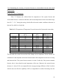
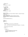
Table 3.2 shows the collected data in testing the accuracy of the temperature measurement of the
device to the digital thermometer. The use of blower allowed the temperature in the box to be
controlled. Based on Table 3.2, the two measurements produced almost the same value for every
trial resulting in small percentage difference. This indicates that the device can produce accurate
measurements of the temperature like the digital thermometer.
Temperature (˚C)
Temperature
True Value vs. Measured Value
50
40
30
20
10
0
Measured Value
(°C)
True Value (°C)
1
2
3
4
5 6 7
Trials
8
9 10
Figure No. 3.10 Temperature – True Value vs. Measured Value
37
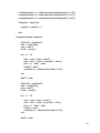
Relative Humidity:
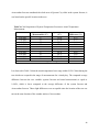
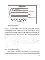
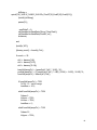
As shown in Table 3.3, most of the readings showed a 100% relative humidity. The relative
humidity is based on the location and on the condition of the atmosphere. A high percentage
relative humidity indicates that the air is holding the maximum water it can hold at the current
temperature and any additional moisture will result in condensation. If the measured relative
humidity is low, it indicates that the atmosphere in the area is dry and can hold more moisture at
that value of temperature. Results show that when the temperature decreases, the relative
humidity goes up due to the small amount of moisture that cooler air can hold for the current
temperature and vice versa (NASA, 2013).
Table No. 3.3 Tabulated Data for Relative Humidity
TRIAL
1
2
3
4
5
6
7
8
9
10
Date & Time
Aug 19, 2013
12:00 AM
3:00 AM
5:00 AM
11:00 AM
2:00 PM
5:00 PM
6:00 PM
7:00 PM
10:00 PM
11:00 PM
Measured Value
(%)
100
100
100
100
100
100
100
100
100
100
True Value
(%)
99
99
100
100
100
100
99
96
100
100
Percentage
Difference (%)
1.0050%
1.0050%
0%
0%
0%
0%
1.0050%
4.0816%
0%
0%
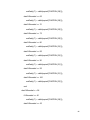
Figure 3.11 presents the differences between the measured and true values of humidity. These
differences are within the acceptable range of values since small differences are calculated. This
proves that the humidity sensor used to measure the parameter in the device produced almost
same performance in measuring humidity as that of the Accuweather. The Accuweather website
stated that it provides a commercially accepted measurement of certain parameters which can be
used for testing purposes.
38
Humidity (%)
Relative Humidity
True Value vs. Measured Value
120
100
80
60
40
20
0
Measured Value
(%)
True Value (%)
1 2 3 4 5 6 7 8 9 10
Trials
Figure No. 3.11 Relative Humidity – True Value vs. Measured Value
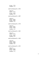
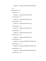
Pressure:
Atmospheric pressure is defined as the force per unit area exerted against a surface by the weight
of the air molecules above that surface (WW2010,2010). The measured and true value of
pressure change only in small part due to the fact that this parameter does not easily alter its
value unlike other parameters. The percentage difference in each trial is close to zero percent,
suggesting that the device can accurately assess the pressure in a given location.
Table No. 3.4 Tabulated Data for Pressure
TRIAL
1
2
3
4
5
6
7
8
9
10
Measured Value
(kPa)
100.9295
100.9297
100.9297
100.9300
100.9381
100.9381
100.9381
100.9382
1009382
100.9382
True Value
(kPa)
100.9
100.9
100.9
100.9
100.9
100.9
100.9
100.9
100.9
100.9
Percentage Difference
(kPa)
0.02923%
0.02943%
0.02943%
0.0297%
0.0378%
0.0378%
0.0378%
0.0379%
0.0379%
0.0379%
39
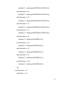
Figure 3.12 proved that the measured value and true value are almost equal and the percentage
acquired in the percent difference does not contribute significantly to the trend of the
measurement of pressure. A constant value of about 100.9 for air pressure was noted during the
time of the testing which indicates that precipitation is less likely. Otherwise, if the measured
pressure is lower, there is an indication that a low pressure system or front is approaching.
Pressure (kPa)
Pressure
True Value vs. Measured Value
120
100
80
60
40
20
0
Measured Value
(kPa)
True Value (kPa)
1 2 3 4 5 6 7 8 9 10
Trials
Figure No. 3.12 Pressure – True Value vs. Measured Value
40
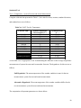
3.4.2 Determining the Accuracy of System Forecasts to Accuweather Forecasts and Actual
Measurements
Hourly Forecasts of Temperature
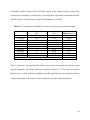
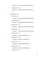
Table 3.5 illustrates the collected data for temperature of the system forecast and
Accuweather forecast. As shown in the table, the forecast temperatures in the Accuweather range
from 24 C° - 31 C° during the testing, which reflect the actual weather condition at that time in
Quezon City which is a cloudy day.
Table No. 3.5 Comparison of Temperature Forecast between the System and Accuweather
Forecast Time
2:00 PM
3:00 PM
4:00 PM
5:00 PM
6:00 PM
7:00 PM
8:00 PM
9:00 PM
10:00 PM
11:00 PM
Accuweather Forecast
System Forecast
(C° )
(C° )
29
26.86
29
27.22
29
27.18
31
27.18
29
27.08
28
26.86
26
26.78
24
26.71
26
26.60
26
26.54
Average Percentage Difference:
Percent
Difference (%)
7.66
6.33
6.48
13.13
6.85
4.16
2.96
10.69
2.28
2.06
6.26
The data under the system forecast show little changes on its temperature forecast because the
estimation of values depends on the actual measurement of the temperature on the area of testing
and historical data. The system forecast increases its value if and only if the present estimated
forecast value is lower than the actual temperature of the area. Otherwise, the system forecast
decreases. A value of 6.26 was computed for the average percentage difference of the 10 trials in
which it does not affect the capability of KF as an algorithm for weather forecasting since the
41
Accuweather forecast considered the whole area of Quezon City while in the system forecast, it
was based on the specific location in the area.
Table No. 3.6 Comparison of System Temperature Forecast to Actual Temperature
Measurement
Forecast Time
2:00 PM
3:00 PM
4:00 PM
5:00 PM
6:00 PM
7:00 PM
8:00 PM
9:00 PM
10:00 PM
11:00 PM
Actual Temperature
System Forecast
Measurement (C° )
(C° )
27
26.86
29
27.22
27
27.18
27
27.18
27
27.08
27
26.86
27
26.78
26
26.71
26
26.60
26
26.54
Average Percentage Difference:
Percent
Difference (%)
0.52
6.33
0.66
0.66
0.30
0.52
0.82
2.69
2.28
2.06
1.684
It is observed in Table 3.6 that the actual temperature has a range within 26-29 Celsius during the
test which was accepted in the range of measurements for a cloudy day. The computed average
difference between the two variables (system forecast and actual measurement) is equal to
1.684%, which is lower compared to the average difference of the system forecast and
Accuweather forecast. These slight differences were acceptable since the location of the test was
not on the same location of the weather station of Accuweather.
42
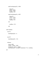
Temperature
35
Temperature (C° )
30
25
Accuweather
Forecast (C° )
20
15
System Forecast (C°
)
10
5
Actual Temperature
Measurement (C° )
0
Forecast Time
Figure No. 3.13 Temperature
Figure 3.13 presents the visual representation of the system forecast, and the Accuweather
forecast and, actual measurement. It shows that the system forecast is close to the actual
measurement at any given time during the time of testing compared to the Accuweather forecast.
It is observed that the time between 2:00 PM to 11:00 PM, the system forecast temperature (red
line) showed an increasing change in its value considering its previous value from the previous
hour. It is caused by the measured temperatures, which is essential in calculating the forecast as
discussed earlier in this chapter. However, the Accuweather forecast showed fluctuations in its
temperature forecast resulting to an observation that during the test, the system forecast values
were closer to the actual measurements.
Hourly Forecasts of Relative Humidity
Relative humidity is an important weather parameter used in forecasting weather.
Humidity indicates the possibility of dew, fog or precipitation. When the recorded measurement
43
of humidity is high, it makes people feel hotter outside in the summer because it reduces the
effectiveness of sweating to cool the body by preventing the evaporation of perspiration from the
skin. This effect is calculated in a heat index table (McEntee et. al.,2009)
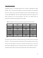
Table No. 3.7 Comparison of Humidity Forecast between the System and Accuweather
Forecast Time
2:00 PM
3:00 PM
4:00 PM
5:00 PM
6:00 PM
7:00 PM
8:00 PM
9:00 PM
10:00 PM
11:00 PM
Accuweather Forecast
System Forecast
(% )
(% )
68
88.11
66
73.23
71
90.09
64
89.25
69
85.58
75
92.87
79
91.42
93
96.89
90
97.17
84
98.45
Average Percent Difference:
Percent
Difference (%)
25.76
10.39
23.70
32.95
21.45
21.29
14.58
4.10
7.66
15.84
17.772
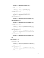
Table 3.7 shows the forecasts from two different sources: the Accuweather site and the system
using KF algorithm. The average difference calculated is equal to 17.772%, which is relatively
high. However, it did not affect the capability of the KF algorithm since, the study focused more
on the determination of the accuracy between system forecast and actual measurement.
44
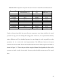
Table No. 3.8 Comparison of System Humidity Forecast to Actual Humidity Measurement
Forecast Time
2:00 PM
3:00 PM
4:00 PM
5:00 PM
6:00 PM
7:00 PM
8:00 PM
9:00 PM
10:00 PM
11:00 PM
Actual Humidity
System Forecast
Measurement (%)
(%)
88
88.11
69
73.23
94
90.09
88
89.25
83
85.58
88
92.87
88
91.42
94
96.89
94
97.17
94
98.45
Average Percent Difference:
Percent
Difference (%)
0.12
5.95
4.25
1.41
3.06
5.39
3.81
3.03
3.32
4.62
3.496
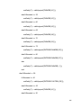
The system forecast and actual measurement for relative humidity were recorded and tabulated
as shown in Table 3.8. The percentage difference included in the table depicts how much the
system forecast differs from the actual data. Based on the calculation, small values of differences
were recorded which means that the system forecasts are almost equal to the actual
measurements at any given time. Moreover, the average percent difference recorded is equal to
3.496%, which was acceptable and the results proved that the Kalman filter can be applied as an
algorithm for weather forecasting. Figure 3.14 shows the differences between the system forecast
to the Accuweather forecast and actual measurements. It was easily observed that the system
forecast were almost closer to the actual value compared to the Accuweather forecast at any
given of time during the testing period.
45
Relative Humidity
120
Relative Humidity (%)
100
80
Accuweather
Forecast
60
System Forecast
40
Actual Humidity
Measurement (%)
20
0
Forecast Time
Figure No. 3.14 Relative Humidity
46
Hourly Forecasts of Pressure
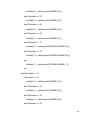
Atmospheric pressure is an important parameter that is essential in monitoring the weather
condition. Table 3.9 presents that the differences in hour-to-hour changes in the atmospheric
pressure are caused by the movement and development of pressure systems affecting the country
very often (MET ÉIREANN). These forecasts proved that the pressure did not change its value
quickly compared to the two previous parameters. Thus, there is no available forecast on
pressure for all weather forecast companies like Accuweather.
Table 3.9 Comparison of Pressure Forecast between the System and Accuweather
Forecast Time
2:00 PM
3:00 PM
4:00 PM
5:00 PM
6:00 PM
7:00 PM
8:00 PM
9:00 PM
10:00 PM
11:00 PM
Accuweather Forecast
System Forecast
(kPa)
(kPa)
101.3
100.79
101.2
100.82
101.1
100.80
101.0
100.80
101.0
100.84
101.1
100.85
101.1
100.89
101.2
100.92
101.3
100.92
101.3
100.94
Average Percentage Difference:
Percent
Difference (%)
0.50
0.38
0.30
0.20
0.16
0.25
0.21
0.28
0.38
0.36
0.302
The system forecast on pressure were almost equal to the Accuweather forecast as observed in
the table 3.9. The present measurement of the pressure affects the prognosis for the next hour.
Thus, there are small difference between the Accuweather and System Forecast. Also, the test
showed that the algorithm may reach a certain point wherein it will be difficult to converge or
estimates the present estimate value due to the consistent values in the measured parameters.
47
Table No. 3.10 Comparison of System Pressure Forecast to Actual Pressure Measurement
Forecast Time
2:00 PM
3:00 PM
4:00 PM
5:00 PM
6:00 PM
7:00 PM
8:00 PM
9:00 PM
10:00 PM
11:00 PM
Actual Pressure
System Forecast
Measurement (%)
(%)
101.2
100.79
101.1
100.82
101.0
100.80
101.0
100.80
101.1
100.84
101.1
100.85
101.2
100.89
101.3
100.92
101.3
100.92
101.3
100.94
Average Percentage Difference:
Percent
Difference (%)
0.41
0.28
0.20
0.20
0.26
0.25
0.31
0.38
0.38
0.36
0.303
Similar to the previous table, the system forecasts on pressure were almost similar to the actual
pressure for any given time during the testing period. In this test, it is expected that relatively
minor differences will be calculated pressure does not change its value as quickly as other
parameters do. As a result, this visual representation of the differences between the system
forecast to the Accuweather forecast and actual measurements were almost equal to each other as
shown in Figure 3.15. These data proved that using the Kalman filter algorithm, the forecast for
pressure are similar to what Accuweather forecasts produced and the measurement of the actual
data.
48
Pressure (kPa)
Pressure
101.4
101.3
101.2
101.1
101
100.9
100.8
100.7
100.6
100.5
Accuweather Forecast
(kPa)
System Forecast (kPa)
Actual Pressure
Measurement (kPa)
Forecast Time
Figure No. 3.15 Pressure
49
Statistical Tool
Test 1: Temperature – System Forecast and Actual Measurement
Using the collected data presented in Table 3.5, the value for mean, variance, standard deviation,
and standard error are as follows:
Table No. 3.11 T-Test for Temperature
Forecast Time
2:00 PM
3:00 PM
4:00 PM
5:00 PM
6:00 PM
7:00 PM
8:00 PM
9:00 PM
10:00 PM
11:00 PM
Mean
Standard Deviation
Standard Error Mean
Actual Temperature
Measurement (C° )
27
29
27
27
27
27
27
26
26
26
26.9
0.8756
0.277
System Forecast
(C° )
26.86
27.22
27.18
27.18
27.08
26.86
26.78
26.71
26.60
26.54
26.901
0.2505
0.079
A two-sided t-test is appropriate to use in determining the difference in the average temperature
measurements of system forecasts and Accuweather forecasts. The hypotheses for this test are as
follows:
Null Hypothesis: The mean temperature of the weather condition is same for the two
measurements: system forecast and actual measurements.
Alternative Hypothesis: The mean temperature of the weather condition differs for the
two measurements: system forecast and actual measurements.
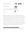
The computation of important parameters are shown below:
50
Standard Error of the Difference (se):
√
√
*
+
Degrees of Freedom (DF) :
(
)
(
)
95% Confidence Interval for the Difference: ( -0.6427 , 0.6407 )
̅
T- Value:
̅
√
P Value:
Observation: A two tailed unequal variance test was conducted to determine the difference of
the temperature forecast produced by the system and actual measurement. The result showed that
there was not a significant difference between the system forecast (M = 26.901; SD = 0.2505)
and the actual measurement (M = 26.9; SD = 0.8756); two sample t (10) = -0.0035, p= 0.9972.
The direction of the difference in the sample means is reflected by the sign (positive or negative)
of the t-value. At the 0.05 significance level and 95% confidence level, it turned out that the null
hypothesis is true so fail to reject the null hypothesis. The mean temperature of the weather
condition is same for the two measurements: system forecast and actual measurements.
Test 2: Relative Humidity – System Forecast and Actual Measurement
The value for mean, variance, standard deviation, and standard error for the two sources are as
follows:
51
Table No. 3.12 T-Test for Relative Humidity
Forecast Time
2:00 PM
3:00 PM
4:00 PM
5:00 PM
6:00 PM
7:00 PM
8:00 PM
9:00 PM
10:00 PM
11:00 PM
Mean
Standard Deviation
Standard Error Mean
Actual Humidity
Measurement (%)
88
69
94
88
83
88
88
94
94
94
88
7.6739
2.427
System Forecast
(%)
88.11
73.23
90.09
89.25
85.58
92.87
91.42
96.89
97.17
98.45
90.306
7.3372
2.32
The hypotheses for this test are as follows:
Null Hypothesis: The mean relative humidity of the weather condition is same for the
two measurements: system forecast and actual measurements.
Alternative Hypothesis: The mean relative humidity of the weather condition differs for
the two measurements: system forecast and actual measurements.
The computation of important parameters are shown below:
Standard Error of the Difference (se):
√
√
*
+
Degrees of Freedom (DF) :
(
)
(
)
95% Confidence Interval for the Difference: ( -9.3894 , 4.7774 )
̅
T- Value:
̅
√
52
P Value:
Observation: A two tailed unequal variance test was conducted to determine the difference of
the relative humidity forecast produced by the system and actual measurement. The result
showed that there was not a significant difference between the system forecast (M = 90.306; SD
= 7.3372) and the actual measurement (M = 88; SD = 7.6739); two sample t (17) = -0.6868,
p= 0.5014. The direction of the difference in the sample means is reflected by the sign (positive
or negative) of the t-value. At the 0.05 significance level and 95% confidence level, it turned out
that the null hypothesis is true so fail to reject the null hypothesis. The mean relative humidity of
the weather condition is same for the two measurements: system forecast and actual
measurements
Test 3: Pressure – System Forecast and Actual Measurement
The value for mean, variance, standard deviation, and standard error for the two sources are as
follows:
Table No. 3.14 T-Test for Pressure
Forecast Time
2:00 PM
3:00 PM
4:00 PM
5:00 PM
6:00 PM
7:00 PM
8:00 PM
9:00 PM
10:00 PM
11:00 PM
Mean
Standard Deviation
Standard Error Mean
Actual Pressure
Measurement (%)
101.2
101.1
101.0
101.0
101.1
101.1
101.2
101.3
101.3
101.3
101.16
0.1174
0.037
System Forecast
(%)
100.86
100.97
100.90
100.90
100.97
101.01
101.20
101.23
101.23
101.23
101.05
0.1546
0.049
53
The hypotheses for this test are as follows:
Null Hypothesis: The mean pressure of the weather condition is same for the two
measurements: system forecast and actual measurements.
Alternative Hypothesis: The mean pressure of the weather condition differs for the two
measurements: system forecast and actual measurements.
The computation of important parameters are shown below:
Standard Error of the Difference (se):
√
√
*
+
Degrees of Freedom (DF) :
(
)
(
)
95% Confidence Interval for the Difference: ( -0.0190 , 0.2390 )
̅
T- Value:
̅
√
P Value:
Observation: A two tailed unequal variance test was conducted to determine the difference of
the pressure forecast produced by the system and actual measurement. The result showed that
there was not a significant difference between the system forecast (M = 101.05; SD = 0.1546)
and the actual measurement (M = 101.16; SD = 0.1174); two sample t (18) = 1.7918, p=
0.0900. At the 0.05 significance level and 95% confidence level, it turned out that the null
hypothesis is true so fail to reject the null hypothesis. The mean pressure of the weather
condition is same for the two measurements: system forecast and actual measurements.
54
Conclusions
A measuring and monitoring device for weather parameters such as temperature, pressure
and, relative humidity is designed and implemented in this study. The objective is achieved by
using a sensor for each parameter and is integrated to the microcontroller. Such sensors are the
LM35 for temperature, capacitive humidity kit for humidity, and MPX114AP for measuring the
pressure. Zigbee technology is also included which allows the transmission of measurements
wirelessly from the device to the laptop or PC. Also, PIC16F877A microcontroller is used for
collecting and processing of the gathered measurements. Since the device is real time, it sends
measurements every 10 seconds.
The Kalman Filter Algorithm is proposed and applied by the researchers to provide
weather forecast. It is applied and implemented using MATLAB based on its equations to
perform the correction and prediction state. This algorithm uses two data, historical and present
data. The combination of the past and present information in Kalman filter produced possible
estimate of the parameters for the prediction of the next state of weather condition.
The program developed for Kalman Filter Algorithm required the system to be trained by
inputting the 80% available data sets or the historical data. These data are gathered in
Accuweather and presented in a CSV file format. The remaining 20% available data are used in
the validation of the system. A high percentage of available data are allocated in the historical
data in order to fully develop the system in the given set of measurements for each parameter.
The testing of the system is divided into two parts: determining the accuracy of
measurements of the device and the forecast produced by the system using KF algorithm. The
results of the first part of the test show that the sensors used for measuring temperature, pressure
and relative humidity produced almost the same measurements as the instruments used for
55
measuring the actual value of the said parameters. Small differences are recorded in the
percentage difference of the actual value to the experimental value for each trial in each
parameter which leads to a conclusion that the device is capable of measuring and monitoring
weather parameters in a specific location. The second part of the testing focused on determining
the accuracy of Kalman filter in forecasting. The calculation of percentage difference and use of
statistical tool such as t-test allowed the determination of the difference of the system forecast to
the Accuweather forecast and to the actual measurement. Based on the results, it showed that
both system forecasts and actual measurements are almost equal which implies that Kalman
Filter can be used as an algorithm for weather forecasting.
An application program is developed to provide access to the general public on the
predicted values by incorporating an Android application and text using GSM technology on the
system. The Android application allowed the person to monitor the changes on the weather
forecasts on their mobile phone. The Bluetooth has successfully allowed the transmission of data
wirelessly from the computer to mobile phone. On the other hand, in case of emergency, a
warning message through GSM technology is used in the system to inform the person. A
command button is displayed in the graphical user interface (GUI) of the MATLAB program
which allows the operator to control the sending of text messages for emergency purposes only.
56
References
Dhar S., et.al, "A Complete Simulation Of Intra Vehicle Link Through Best PossibleWireless
Network", IJCEE., vol. 2, no. 4, pp. 674, Aug. 2010
Esme
B.
(2009).
Kalman
Filter
for
Dummies
http://bilgin.esme.org/BitsBytes/KalmanFilterforDummies.aspx
[Online].
Available:
Faragher R. "Understanding the Basis of the Kalman Filter via a Simple and Intuitive
Derivation" [Lecture Notes]. Signal Processing Magazine, IEEE , vol.29, no.5, pp.128-132, Sept.
2012 doi: 10.1109/MSP.2012.2203621
Microchip PIC16F87XA 28/40/44-Pin Enhanced Flash Microcontrollers, Microchip Technology
Inc., USA, 2012
Mastro M. (2013). Financial Derivative and Energy Market Valuation. John Wiley & Sons, Inc.
DOI: 10.1002/9781118501788.ch7
NASA Official. (2013). Data Enhanced Investigations for Climate Change Education (DICCE)
Giovanni Help Page [Online]. Available: http://disc.sci.gsfc.nasa.gov/giovanni/additional/usersmanual/DICCE_Help
Rountree D.M. (2010). Paranormal Technology: Understanding the Science of Ghost Hunting.
iUniverse. 1663 Liberty Drive Bloomington, IN 4703
Scaringe R. P. (2007). Indoor Air Quality and Mold Remediation. Mainstream Engineering
Corporation, 200 Yellow Place, Rockledge, Florida 3295
Scheneider Electric Industries SAS. (2011). Zigbee - Setting Standards for Energy-Efficient
Control Networks. Volume 1 (1), 11-12
Taranovich S. (2011). Humidity Sensors and Signal Conditioning Choices. [Online]. Available:
http://www.digikey.com/us/en/techzone/sensors/resources/articles/humidity-sensors-and-signalconditioning-choices.html (Accessed: September 25, 2013)
The MathWorks Inc.(2013). MATLAB Product Description - The Language of Technical
Computing [Online]. Available: http://www.mathworks.com/help/matlab/learn_matlab/productdescription.html
WW2010 Department of Atmospheric Sciences. University of Illinois at Urbana-Champaign.
"Atmospheric
Pressure"
[Online].
Available:
http://ww2010.atmos.uiuc.
edu/(Gh)/guides/mtr/prs/def.rxml
57
Chapter 4
CONCLUSIONS
A measuring and monitoring device for weather parameters such as temperature, pressure
and, relative humidity is designed and implemented in this study. The objective is achieved by
using a sensor for each parameter and is integrated to the microcontroller. Such sensors are the
LM35 for temperature, capacitive humidity kit for humidity, and MPX114AP for measuring the
pressure. Zigbee technology is also included which allows the transmission of measurements
wirelessly from the device to the laptop or PC. Also, PIC16F877A microcontroller is used for
collecting and processing of the gathered measurements. Since the device is real time, it sends
measurements every 10 seconds.
The Kalman Filter Algorithm is proposed and applied by the researchers to provide
weather forecast. It is applied and implemented using MATLAB based on its equations to
perform the correction and prediction state. This algorithm uses two data, historical and present
data. The combination of the past and present information in Kalman filter produced possible
estimate of the parameters for the prediction of the next state of weather condition.
The program developed for Kalman Filter Algorithm required the system to be trained by
inputting the 80% available data sets or the historical data. These data are gathered in
Accuweather and presented in a CSV file format. The remaining 20% available data are used in
the validation of the system. A high percentage of available data are allocated in the historical
data in order to fully develop the system in the given set of measurements for each parameter.
The testing of the system is divided into two parts: determining the accuracy of
measurements of the device and the forecast produced by the system using KF algorithm. The
results of the first part of the test show that the sensors used for measuring temperature, pressure
58
and relative humidity produced almost the same measurements as the instruments used for
measuring the actual value of the said parameters. Small differences are recorded in the
percentage difference of the actual value to the experimental value for each trial in each
parameter which leads to a conclusion that the device is capable of measuring and monitoring
weather parameters in a specific location. The second part of the testing focused on determining
the accuracy of Kalman filter in forecasting. The calculation of percentage difference and use of
statistical tool such as t-test allowed the determination of the difference of the system forecast to
the Accuweather forecast and to the actual measurement. Based on the results, it showed that
both system forecasts and actual measurements are almost equal which implies that Kalman
Filter can be used as an algorithm for weather forecasting.
An application program is developed to provide access to the general public on the
predicted values by incorporating an Android application and text using GSM technology on the
system. The Android application allowed the person to monitor the changes on the weather
forecasts on their mobile phone. The Bluetooth has successfully allowed the transmission of data
wirelessly from the computer to mobile phone. On the other hand, in case of emergency, a
warning message through GSM technology is used in the system to inform the person. A
command button is displayed in the graphical user interface (GUI) of the MATLAB program
which allows the operator to control the sending of text messages for emergency purposes only.
59
Chapter 5
RECOMMENDATIONS
The study focused on the implementation and testing of Kalman filter as an algorithm for
predicting weather condition. It is proposed that the testing of the system must be performed and
exercised on the exact location where the weather station of the data to be compared is located.
This is to have a more appropriate observation and comparisons on the system forecast to the
forecast of the chosen weather station.
In Chapter 3 of this study, it is noted that the KF algorithm is a recursive algorithm which
denotes that the calculation of the present value is dependent upon the previous calculated value
of it. Thus, the system must have the capability to store the previous value for each parameter
used. It is reached solely by throwing the whole system turned on for the continuous simulation.
For the future researchers who will continue to improve this study, it is recommended that a
database must be implemented in MATLAB to achieve ease of usage of the system.
Furthermore, the device capability to send information efficiently and faster can be
achieved by embracing new technologies as a substitute for the components employed in this
study. Some technologies for wireless data communication can be used as a substitute for the
GSM technology and Bluetooth such as WI-Fi. The standard Zigbee used in the device can be
upgraded to a Pro Zigbee, which has more advantages like faster transmission of measured data
for the data logger purposes. This will allow the user to observe the changes easily occurred on
each parameter since the system exhibits real time.
60
REFERENCES
Annenberg Learner and Foundation. 2013. Weather What forces affect our weather?.[Online]. Available:
http://www.learner.org/interactives/weather/ forecasting2.html (Accessed: March 2, 2013)
Graham Hesketh, ―Kalman Filters for Fun‖, Information Engineering, Rolls-Royce Strategic Research
Center, Group, 2000
Greg Welch, Gary Bishop, "An Introduction to the Kalman Filter", University of North Carolina at
Chapel Hill Department of Computer Science, 2001
Grewal M. and Andrews A.P, ―Kalman Filtering: Theory and Practice using MATLAB, 3 rd edition, John
Wiley & Sons Inc., 2008.
Jean de DieuNiyigaba.VariationalKalman Filter.[Online]. Available: http://personal.lut.fi/98C0C551E3C9-4CB2-A0A0-78B5374C87C8/FinalDownload/DownloadId1868387BF6482526F6A1B6A1DECFFC31/98C0C551-E3C9-4CB2-A0A078B5374C87C8/wiki/lib/exe/fetch.php/en/technomathematics/time_series_research/start/variational_kalm
an_filter.pdf
Kleinbauer, R., ―Kalman Filtering Implementation with MatLab,‖ Field of Study Geodesy and
Geoinformatics at Universitat Stuttgart, Helsinki, 2004.
Lee Lerner, K. and Wilmoth Lerner, B., ―Other Forecasting Methods‖ in World of Earth Science. The
Gale Group, Inc., 2003.
Manolis Anadranistakis, et al. ―Correcting Temperature and Humidity Forecasts using Kalman Filtering:
Potential for Agricultural Protection in Northern Greece‖. Nevrokopi, Greece, 2004
McKemy D. et al. Climate Education for K-12: Instruments. [Online] Available: http://www.ncclimate.ncsu.edu/edu/k12/.instruments (Accessed: March 2, 2013)
Nilofer
Mehta,
―Kalman
Filtering
of
Sensor
Data‖
http://web.cs.dal.ca/~reilly/CSCI6609/seminars/sensors_kalman_filters.pdf
[Online].
Available:
Noordin K., Oon C. and M. Ismail. ―A Low-Cost Microcontroller-based Weather Monitoring System‖.
Department of Electrical Engineering, Faculty of Engineering, University of Malaya, 50603. Kuala
Lumpur, Malaysia.
Segaran, Toby, ―Programming Collective Intelligence: Building Smart Web 2.0 Applications,‖ O’Reilly,
2007.
Simeonov, I., Killifarev H. and Ilarionov R. , ―Embedded System for Short-term Weather Forecasting,‖
CompSysTech, 2006.
The Daily Weather Forecast. [Online]. Available: http://kidlat.pagasa.dost.gov.ph/genmet/pwf.html
Yu, X., Efe, M. and Kaynak O., ―A Backpropagation Learning Framework for Feedforward Neural
Networks,‖ Faculty of Informatics and Communication, Central Queensland University, Australia, 2001.
61
APPENDIX A
Operation’s Manual
1. System Requirement
 Operating System: Windows 7 64-bit
2. Installation Procedure
Installing the software for the drive:
1. Open the Other Software folder in the provided CD.
2. Double click the CH341SER64Bit.
3. A window will be displayed like as shown below.
Figure No. 3.16 Driver Setup(x64)
4. Click the Install button.
5. A prompt will be displayed telling that the drive is successfully completed.
62
Installing the MATLAB software:
1. Insert the CD for installing MATLAB.
2. Double click setup.
3. A window will be displayed similar to the figure below. See Figure 3.17.
Figure No. 3.17 MathWorks Installer
4. Choose Install manually without using the Internet. Then, click Next.
5. In the License Agreement, choose Yes. Then, click Next.
6. In the File Installation Key window, choose ―I have the File Installation for my
license:‖
Figure No. 3.18 File Installation Key Window
63
7. In order to get the installation key, open the crack folder in the CD. Open the
notepad file named ―install‖.
Figure No. 3.19 File Installation Key
8. Copy the file installation key on the space provided. Then, click Next.
9. Choose ―Typical‖. Click Next.
10. Specify the folder where you want to install MATLAB. Click Next.
Figure No. 3.20 Folder Selection
64
11. Click Install. The installation procedure will start.
Figure No. 3.21 Installation Confirmation
12. After installing, activate MATLAB and click Next. After that, click Finish.
Figure No. 3.22 Installation Complete
65
Installing the Android application of Kalman Filter:
1. Connect your cellphone to the PC or laptop via Bluetooth.
Note: Most laptops and desktops do have Bluetooth. If yours doesn’t, a USB
Bluetooth adapter can be used.
2. Enable Bluetooth on your cell phone.
3. Go to Control Panel under the Start Menu and then go to the Hardware and Sound.
From there, choose Devices and Printers and click Add a Bluetooth device as shown
in the Figure 3.23 below.
Figure No. 3.23 Add a Bluetooth Device
4. Scan for devices on your PC or laptop and choose your device name.
Note: Make sure that your Bluetooth status is discoverable in order for the computer
to detect your device.
5. Once your device is paired with your PC or laptop, transfer the Kalman. Ape file
provided to your cell phone.
Note: Open the Apps folder, and then go to Objects. Right-click on the Kalman.apk
file and then send to Bluetooth device. See Figure 3.24.
66
Figure No. 3.24 Kalman.apk
6. Open the Kalman.apk file on your cellphone.
Note: Be sure to allow your mobile phone in installing non-Market applications. Go
to Settings->Applications->Unknown sources.
7. A prompt will ask you to choose from the two options displayed in your mobile
phone to complete the action. Such options include Package installer and Verify and
Install. Choose Package Installer.
Figure No. 3.25 Package Installer
67
8. After that, the system will verify the installation of the application. Click the Install
button and wait until the installation is completed.
Figure No. 3.26 Kalman Installation
9. Two options will then be showed on your phone’s screen: Open or Done. Open
button must be selected to open the android application and Done button to exit.
Note: Once the android application is opened in your mobile phone, it will turn on
your Bluetooth connection to let the other devices (laptop or PC) to connect. Figure
3.27 shows the GUI of the android application.
68
Figure No. 3.27 Kalman GUI
Creating COM port for Bluetooth
1. Once your mobile phone is paired on the PC or laptop, find and click the Bluetooth
icon. Select the Open Settings to display the current settings of the Bluetooth on your
laptop or PC.
Figure No. 3.28 Opening the Bluetooth Settings
69
2. The Bluetooth Settings will appear as shown in Figure 3.29. Click the COM ports tab.
Figure No. 3.29 Bluetooth Settings Window
3. In the COM ports tab, click the Add button.
Figure No. 3.30 COM Ports
4. The Add COM port window will be displayed. Verify that the radio button for
Incoming (device initiates the connection) is selected. Then click OK button.
70
Figure No. 3.31 Add COM Port
5. A verification message will be displayed in the Taskbar informing that the device
driver software was installed successfully and the COM port for Bluetooth is
displayed. Then click OK in the Bluetooth Settings window.
Figure No. 3.32 Standard Serial over Bluetooth link
71
Note: This COM port will be used and declared in the MATLAB program for Weather
Prediction using Kalman Filter. Assign this port number in the COM port declaration of
the code.
Figure No. 3.33 Modified COM Port
3. User’s Manual
1. Connect the USB to serial port in the serial port of the device (the small one). See
figure below.
Figure No. 3.34 Zigbee Serial Connection
2. In the same device, connect the two USB cable to the USB port of the PC or laptop.
Be sure that the driver is installed properly. The red LED will blink to signify that it is
ready to use.
72
Figure No. 3.35 Complete Set-up of Zigbee
3. Plug the other device (the larger one). A red LED will light up first and then the green
LED will start to blink. Wait until the light of the green LED is steady which signifies
that the device is ready to use, otherwise it is in OFF mode. To turn it ON, switch the
toggle switch at the back of the device.
Figure No. 3.36 Device for Measuring Weather Parameters
73
4. Open the MATLAB -> Click File menu -> Click New -> Select GUI -> Select Open
Existing GUI then browse the Fig-File of the program. The program is provided on
the CD in the Wireless Weather folder.
Figure No. 3.37 Opening an Existing GUI file
5. A window will appear like the figure below.
74
Figure No. 3.38 .fig file
6. To open the M-file, right click the Start Data Acquisition button, then select View
Callbacks then Callback.
Figure No. 3.39 M-file
7. Click the Run button.
75
Figure No. 3.40 Run Button
8. Select a Raw Data CSV in order for the program to run.
Figure No. 3.41 Selecting Raw Data
Note: A CSV file consists of any number of records, separated by line breaks of
any kind; each record consists of fields, separated by some other character or
string, most commonly a literal comma or tab (Babylons’ English Dictionary).
9. The GUI is shown below.
76
Figure No. 3.42 .fig File for Kalman Filter
10. You can choose any parameter you want to be displayed in the graph provided. Click
the Start Data Acquisition. After 15 seconds, the measurements and the predicted
value for the weather parameters; temperature, pressure and humidity will be
displayed. Each parameter will have ten (10) samples.
4. Troubleshooting Guides and Procedures
1. Clicking the Start Data Acquisition button in MATLAB doesn’t work
a. First, make sure that the device is plugged in.
b. Check if the serial cable is properly connected to the laptop and to the device.
c. Open the MATLAB and the m-file again.
2. The COM port used in serial connection is not available
a. Make sure that the serial cable is properly connected to your PC or laptop and
the device.
b. Verify the COM port number in the Device Manager by following the steps
provided in the installation of Bluetooth.
c. In the m-file, locate the COM port number used. Change it to the COM port
number displayed in the pop-up window in the Taskbar.
d. Run the M-file.
77
3. No COM port number displayed in the Device Manager
a. Make sure that the serial cable is properly connected to your laptop and
device.
b. Reinstall the driver. See the Installation Procedure.
c. Reopen the MATLAB and rerun the m-file.
d. If same problem was encountered, the serial cable is defective. Try using
another serial cable then rerun the m-file.
4. The android application cannot connect to the program via Bluetooth connection or
there is an error occurred while making a connection
a. Quit the android application of Kalman Filter.
b. Restart the mobile phone.
c. Open the android application and reconnect it to the laptop or PC.
d. If the android application is still cannot connect to the laptop or PC, go to the
Bluetooth settings and to the COM Ports tab.
e. Remove the COM port number of the incoming device and add again another
COM port number of the incoming device.
f. Modify the COM port number in the MATLAB program for Kalman filter.
g. Reconnect again the android application to the laptop or PC.
5. The COM port number for Bluetooth connection is not available
a. Check the Bluetooth Settings for the COM port number of the incoming
device.
b. Check the COM port number declared in the MATLAB program.
c. If the COM port number is the same for the previous steps, rewrite again the
COM port number in the MATLAB program and save it.
d. Click the Run button in MATLAB.
5. Error Definitions
1. Unhandled internal error in guidefunc - The error below simply shows that the inputted
COM port number for the serial connection is not available.
78
Figure No. 3.43 Unhandled Internal Error
2. Error using serial/fopen (line 72) – the COM port used for the Bluetooth connection is
not available. The error shown in the figure below displays same port number for the
available and not available port.
Figure No. 3.44 Error on opening serial port
3. Error – the Bluetooth connection of the laptop or PC to the android application in
mobile phone is disconnected.
79
APPENDIX B
M-Files (Codes)
PIC16F877A
Device 16F877A
Declare Xtal = 20
Declare Adin_Res 10
Declare Adin_Tad FRC
Declare Adin_Stime 50
Declare
Declare
Declare
Declare
Hserial_Baud = 9600
Hserial_RCSTA = %10010000
Hserial_TXSTA = %00100100
Hserial_Clear True
Symbol gsmPW = PORTD.5
Symbol gsmIn = PORTD.7
Symbol gsmOut = PORTD.6
Symbol LED01 = PORTD.0
Dim aRead1 As Word
Dim aRead2 As Word
Dim aRead3 As Word
Dim
Dim
Dim
Dim
aReadTemp As Dword
gCtr As Word
uNum1[12] As Byte
myCom As Byte
Dim pTemp[9] As Byte, pPres[9] As Byte, pHum[9] As Byte
ADCON1 = $80
TRISA = $FF
TRISB = $FF
TRISC = $BF
TRISD = $9E
TRISE = $07
DelayMS 50
80
pTemp[8] = 0 : pPres[8] = 0 : pHum[8] = 0
GoSub subs_SMS_Init
HSerOut["U"]
While 1 = 1
HSerIn [Wait("U"), myCom]
Select Case myCom
Case "D"
aReadTemp = 0
For gCtr = 1 To 1000
aRead1 = ADIn 0
aReadTemp = aReadTemp + aRead1
DelayUS 5
Next gCtr
aReadTemp = aReadTemp / 1000
aRead1 = aReadTemp
aReadTemp = 0
For gCtr = 1 To 1000
aRead3 = ADIn 2
aReadTemp = aReadTemp + aRead3
DelayUS 5
Next gCtr
aReadTemp = aReadTemp / 1000
aRead3 = aReadTemp
aRead2 = Counter PORTD.2, 900
HSerOut ["ADC: ",Dec4 aRead3,32,Dec4 aRead1,32,Dec4 aRead2,13]
81
Case "S"
pHum\8]
HSerIn [Wait("_"), Str pTemp\8, Wait("_"), Str pPres\8, Wait("_"), Str
GoSub subs_SMS_Send
HSerOut["U"]
EndSelect
'DelayMS 1000
Wend
subs_SMS_Init:
gsmPW = 1
DelayMS 2500
gsmPW = 0
DelayMS 5000
LED01 = 1
SerOut gsmOut, 84, ["AT",13]
DelayMS 2000
LED01 = 0 : DelayMS 500 : LED01 = 1
SerOut gsmOut, 84, ["AT+CIURC=0",13]
SerIn gsmIn, 84, 1500, subs_SMS_InitFailed,[Wait("OK")]
DelayMS 500
LED01 = 0 : DelayMS 500 : LED01 = 1
SerOut gsmOut, 84, ["AT+CNMI=3,1,0,0,0",13]
SerIn gsmIn, 84, 1500, subs_SMS_InitFailed,[Wait("OK")]
DelayMS 500
LED01 = 0 : DelayMS 500 : LED01 = 1
82
SerOut gsmOut, 84, ["AT+CFUN=1",13]
SerIn gsmIn, 84, 1500, subs_SMS_InitFailed,[Wait("OK")]
DelayMS 500
LED01 = 0 : DelayMS 500 : LED01 = 1
SerOut gsmOut, 84, ["AT+CMGF=1",13]
SerIn gsmIn, 84, 1500, subs_SMS_InitFailed,[Wait("OK")]
DelayMS 500
LED01 = 0 : DelayMS 500 : LED01 = 1
SerOut gsmOut, 84, ["AT+CMEE=0",13]
SerIn gsmIn, 84, 1500, subs_SMS_InitFailed,[Wait("OK")]
DelayMS 500
LED01 = 0 : DelayMS 500 : LED01 = 1
SerOut gsmOut, 84, ["AT+CSDH=0",13]
SerIn gsmIn, 84, 1500, subs_SMS_InitFailed,[Wait("OK")]
DelayMS 500
LED01 = 0 : DelayMS 500 : LED01 = 1
SerOut gsmOut, 84, ["ATE1",13]
SerIn gsmIn, 84, 1500, subs_SMS_InitFailed,[Wait("OK")]
DelayMS 500
LED01 = 0 : DelayMS 500 : LED01 = 0
For gCtr = 10 To 1 Step -1
LED01 = ~LED01
DelayMS 500
Next gCtr
For gCtr = 0 To 10
uNum1[gCtr] = "0"
Next gCtr
83
uNum1[11] = 0
'retrieve admin number
SerOut gsmOut, 84, ["AT+CPBF=",34,"ADMIN",34,13]
SerIn gsmIn, 84, 3500, subs_SMS_InitFailed, [Wait("+CPBF:"),Wait(34),Str
uNum1\11,Wait("OK")]
DelayMS 2000
LED01 = 1
Return
subs_SMS_Send:
sj_SS_Start:
LED01 = 0
For gCtr = 1 To 3
LED01 = ~LED01
DelayMS 500
Next gCtr
LED01 = 1
SerOut gsmOut , 84, ["AT",13]
DelayMS 500
LED01 = 0 : DelayMS 500 : LED01 = 1
SerOut gsmOut , 84, ["AT",13]
DelayMS 500
LED01 = 0 : DelayMS 500 : LED01 = 1
SerOut gsmOut , 84, ["AT+CMGS=",34,Str uNum1\11,34,13]
84
DelayMS 500
LED01 = 0 : DelayMS 500 : LED01 = 1
SerOut
SerOut
SerOut
SerOut
gsmOut,
gsmOut,
gsmOut,
gsmOut,
84,
84,
84,
84,
["Data Results:",13]
["P.Temperature: ", Str pTemp\8,13]
["P.Pressure: ", Str pPres\8,13]
["P.Humidity: ", Str pHum\8,13]
LED01 = 0 : DelayMS 500 : LED01 = 1
SerOut gsmOut , 84, [26]
DelayMS 500
LED01 = 1
sj_SMS_Out:
Return
subs_SMS_InitFailed:
LED01 = 1
While 1 = 1
LED01 = ~LED01
DelayMS 250
Wend
Return
End
In programming the microcontroller, the researchers first define XTAL which serves as the
crystal oscillator of PIC16F877A. It is the oscillator that produces electrical oscillations at a
frequency determined by the physical characteristics of a piezoelectric quartz crystal (The
85
FreeDictionary). After that, they declared the following parameters: Adin_Res 10, Adin_Tad
FRC, and Adin_Stime 50 which signifies a 10-bit result required, FRC as a chosen oscillator
and allows 50µs sample time, respectively.
The next thing that must be implemented is to configure the following input ports declared as
TRISA, TRISB, TRISC, TRISD, and TRISE. After that, the microcontroller would be able to
read the measured data of the following sensors, temperature, pressure and humidity. Then, it
will output the measured values which will then be displayed in the data logger of the
MATLAB GUI.
86
MATLAB
function varargout = WWM(varargin)
gui_Singleton = 1;
gui_State = struct('gui_Name',
mfilename, ...
'gui_Singleton', gui_Singleton, ...
'gui_OpeningFcn', @WWM_OpeningFcn, ...
'gui_OutputFcn', @WWM_OutputFcn, ...
'gui_LayoutFcn', [] , ...
'gui_Callback', []);
if nargin && ischar(varargin{1})
gui_State.gui_Callback = str2func(varargin{1});
end
if nargout
[varargout{1:nargout}] = gui_mainfcn(gui_State, varargin{:});
else
gui_mainfcn(gui_State, varargin{:});
end
handles.output = hObject;
delete(instrfindall);
movegui(hObject,'center');
if(~isdeployed)
cd(fileparts(which(mfilename))); % From Brett
end
set(handles.figure1,'name','Weather Forecast Using Kalman Filter Algorithm');
guidata(hObject, handles);
global AcqFlag;
global grpFlag;
global sendDataF;
sampTotal = 10;
tempVal = zeros(1);
presVal = zeros(1);
humiVal = zeros(1);
%rowData = zeros(sampTotal,3);
sampCtr = 1;
87
grpFlag = 1;
[CSVPath, folder] = uigetfile('*.CSV*', 'Select Raw Data CSV:');
CSVPath = fullfile(folder, CSVPath);
rawData = csvread(CSVPath,1,0);
sDevT = 0.1;
sDevP = 0.1;
sDevH = 0.1;
DataT = rawData(:,1);
DataP = rawData(:,2);
DataH = rawData(:,3);
kRep = size(DataT);
PredT = zeros(kRep);
PredP = zeros(kRep);
PredH = zeros(kRep);
lastPT = 0;
lastPP = 0;
lastPH = 0;
aVar = 0;
pVar = 1;
for i = 1 : kRep
kVar = pVar / (pVar + sDevT);
aVar = aVar + (kVar * (DataT(i) - aVar));
pVar = (1 - kVar) * pVar;
PredT(i) = aVar;
end
lastPT = pVar;
aVar = 0;
pVar = 1;
88
for i = 1 : kRep
kVar = pVar / (pVar + sDevP);
aVar = aVar + (kVar * (DataP(i) - aVar));
pVar = (1 - kVar) * pVar;
PredP(i) = aVar;
end
lastPP = pVar;
aVar = 0;
pVar = 1;
for i = 1 : kRep
kVar = pVar / (pVar + sDevH);
aVar = aVar + (kVar * (DataH(i) - aVar));
pVar = (1 - kVar) * pVar;
PredH(i) = aVar;
end
lastPH = pVar;
h = subplot(1,1,1,'Parent',handles.pnlGrapher);
hold on;
%subplot(1,1);
plot(DataT,'b');
plot(PredT,'r');
legend('Actual Data','Predicted Data');
xlabel('Samples');
ylabel('Temperature (c)');
drawnow;
%axes(h);
%DataAcq Block------------------------------------------------------------s = serial('COM31',...
'BaudRate', 9600,...
'TimeOut',5,...
89
'Terminator',13);
fopen(s);
s.ReadAsyncMode = 'manual';
s2 = serial('COM33',...
'BaudRate', 9600,...
'TimeOut',5,...
'OutputBufferSize',1024,...
'Terminator',13);
fopen(s2);
s2.ReadAsyncMode = 'manual';
%format the table
colNames = {'Temperature','Pressure','Humidity', 'Predicted T', 'Predicted P','Predicted
H','Heat Index'};
colData = {0,0,0,0,0,0,0};
set(handles.tblDataLogs,'data',colData,'ColumnName',colNames);
set(handles.tblDataLogs, 'ColumnWidth', {80 80 80 80 80 80 120});
drawnow;
set(handles.btnGetData,'Enable','on');
AcqFlag = 0;
sendDataF = 0;
while 1 == 1
oras = clock;
myDate = datestr(oras,'mmmm dd, yyyy HH:MM:SS AM');
myTitle = sprintf('Weather Forecast Using Kalman Filter Algorithm - %s', myDate);
set(handles.figure1,'name',myTitle);
if AcqFlag == 1
if sendDataF == 1
set(handles.btnSendData,'String','Sending Data');
set(handles.btnSendData,'Enable','off');
drawnow;
90
btString =
sprintf('US_%08.2f_%08.2f_%08.2f\n',PredT(10),PredP(10),PredH(10));
fprintf(s,btString);
pause(10);
sendDataF = 0;
set(handles.btnSendData,'String','Send Data');
set(handles.btnSendData,'Enable','on');
drawnow;
end
fprintf(s,'UD');
[dummy,count] = fscanf(s,'%s');
if count >= 19
str1 = dummy(5:8);
str2 = dummy(9:12);
str3 = dummy(13:16);
tempVal(sampCtr) = (sscanf(str1,'%d') * 4.88) / 10;
presVal(sampCtr) = ((((sscanf(str2,'%d') * 4.89) / 5000) + 0.095) / 0.009)*2;
humiVal(sampCtr) = sscanf(str3,'%d');
if humiVal(sampCtr) > 7351
% RH < 0 - out of range
humBase = 101;
elseif humiVal(sampCtr) > 7224
%base 0
hUpper = 7351;
hLower = 7224;
humBase = 0;
elseif humiVal(sampCtr) > 7100
%base 10
hUpper = 7224;
91
hLower = 7110;
humBase = 10;
elseif humiVal(sampCtr) > 6976
%base 20
hUpper = 7110;
hLower = 6976;
humBase = 20;
elseif humiVal(sampCtr) > 6853
%base 30
hUpper = 6976;
hLower = 6853;
humBase = 30;
elseif humiVal(sampCtr) > 6728
%base 40
hUpper = 6853;
hLower = 6728;
humBase = 40;
elseif humiVal(sampCtr) > 6600
%base 50
hUpper = 6728;
hLower = 6600;
humBase = 50;
elseif humiVal(sampCtr) > 6468
%base 60
hUpper = 6600;
hLower = 6468;
humBase = 60;
elseif humiVal(sampCtr) > 6330
%base 70
hUpper = 6468;
hLower = 6330;
humBase = 70;
92
elseif humiVal(sampCtr) > 6186
%base 80
hUpper = 6330;
hLower = 6186;
humBase = 80;
elseif humiVal(sampCtr) > 6033
%base 90
hUpper = 6186;
hLower = 6033;
humBase = 90;
else
humBase = 100;
end
switch humBase
case 101
humiVal(sampCtr) = 0;
case 100
humiVal(sampCtr) = 100;
otherwise
freqH = 6660;
freqDiff = hUpper - freqH;
freqInterval = hUpper - hLower;
humiVal(sampCtr) = ((freqDiff / freqInterval) * 10) + humBase;
end
93
rowData(sampCtr,1) = cellstr(num2str(tempVal(sampCtr),'%.2f'));
rowData(sampCtr,2) = cellstr(num2str(presVal(sampCtr),'%.2f'));
rowData(sampCtr,3) = cellstr(num2str(humiVal(sampCtr),'%.2f'));
if sampCtr < sampTotal
sampCtr = sampCtr + 1;
else
%compute Kalman Predictions
[sRW,sCL] = size(PredT);
aVar = PredT(sRW);
pVar = lastPT;
PredT = zeros(1);
for i = 1 : 10
kVar = pVar / (pVar + sDevT);
aVar = aVar + (kVar * (tempVal(i) - aVar));
pVar = (1 - kVar) * pVar;
PredT(i) = aVar;
rowData(i,4) = cellstr(num2str(aVar,'%.2f'));
end
lastPT = pVar;
[sRW,sCL] = size(PredP);
aVar = PredP(sRW);
pVar = lastPP;
PredP = zeros(1);
for i = 1 : 10
kVar = pVar / (pVar + sDevT);
aVar = aVar + (kVar * (presVal(i) - aVar));
pVar = (1 - kVar) * pVar;
PredP(i) = aVar;
rowData(i,5) = cellstr(num2str(aVar,'%.2f'));
end
lastPP = pVar;
94
[sRW,sCL] = size(PredH);
aVar = PredH(sRW);
pVar = lastPH;
PredH = zeros(10);
for i = 1 : 10
kVar = pVar / (pVar + sDevT);
aVar = aVar + (kVar * (humiVal(i) - aVar));
pVar = (1 - kVar) * pVar;
PredH(i) = aVar;
rowData(i,6) = cellstr(num2str(aVar,'%.2f'));
end
lastPH = pVar;
%get Heat Index
for i = 1 : 10
tRounded = round(PredT(i));
hRounded = round(PredH(i));
if tRounded == 27
if hRounded == 40
rowData(i,7) = cellstr(sprintf('CAUTION (27)'));
elseif hRounded == 45
rowData(i,7) = cellstr(sprintf('CAUTION (27)'));
elseif hRounded == 50
rowData(i,7) = cellstr(sprintf('CAUTION (27)'));
elseif hRounded == 55
rowData(i,7) = cellstr(sprintf('CAUTION (28)'));
elseif hRounded == 60
95
rowData(i,7) = cellstr(sprintf('CAUTION (28)'));
elseif hRounded == 65
rowData(i,7) = cellstr(sprintf('CAUTION (28)'));
elseif hRounded == 70
rowData(i,7) = cellstr(sprintf('CAUTION (29)'));
elseif hRounded == 75
rowData(i,7) = cellstr(sprintf('CAUTION (29)'));
elseif hRounded == 80
rowData(i,7) = cellstr(sprintf('CAUTION (30)'));
elseif hRounded == 85
rowData(i,7) = cellstr(sprintf('CAUTION (30)'));
elseif hRounded == 90
rowData(i,7) = cellstr(sprintf('CAUTION (31)'));
elseif hRounded == 95
rowData(i,7) = cellstr(sprintf('CAUTION (31)'));
elseif hRounded == 100
rowData(i,7) = cellstr(sprintf('CAUTION (32)'));
end
elseif tRounded == 28
if hRounded == 40
rowData(i,7) = cellstr(sprintf('CAUTION (28)'));
elseif hRounded == 45
96
rowData(i,7) = cellstr(sprintf('CAUTION (28)'));
elseif hRounded == 50
rowData(i,7) = cellstr(sprintf('CAUTION (28)'));
elseif hRounded == 55
rowData(i,7) = cellstr(sprintf('CAUTION (29)'));
elseif hRounded == 60
rowData(i,7) = cellstr(sprintf('CAUTION (29)'));
elseif hRounded == 65
rowData(i,7) = cellstr(sprintf('CAUTION (30)'));
elseif hRounded == 70
rowData(i,7) = cellstr(sprintf('CAUTION (31)'));
elseif hRounded == 75
rowData(i,7) = cellstr(sprintf('CAUTION (31)'));
elseif hRounded == 80
rowData(i,7) = cellstr(sprintf('CAUTION (32)'));
elseif hRounded == 85
rowData(i,7) = cellstr(sprintf('EXTREME CAUTION (33)'));
elseif hRounded == 90
rowData(i,7) = cellstr(sprintf('EXTREME CAUTION (34)'));
elseif hRounded == 95
rowData(i,7) = cellstr(sprintf('EXTREME CAUTION (35)'));
elseif hRounded == 100
97
rowData(i,7) = cellstr(sprintf('EXTREME CAUTION (36)'));
end
elseif tRounded == 29
if hRounded == 40
rowData(i,7) = cellstr(sprintf('CAUTION (29)'));
elseif hRounded == 45
rowData(i,7) = cellstr(sprintf('CAUTION (29)'));
elseif hRounded == 50
rowData(i,7) = cellstr(sprintf('CAUTION (30)'));
elseif hRounded == 55
rowData(i,7) = cellstr(sprintf('CAUTION (30)'));
elseif hRounded == 60
rowData(i,7) = cellstr(sprintf('CAUTION (31)'));
elseif hRounded == 65
rowData(i,7) = cellstr(sprintf('CAUTION (32)'));
elseif hRounded == 70
rowData(i,7) = cellstr(sprintf('EXTREME CAUTION (33)'));
elseif hRounded == 75
rowData(i,7) = cellstr(sprintf('EXTREME CAUTION (34)'));
elseif hRounded == 80
rowData(i,7) = cellstr(sprintf('EXTREME CAUTION (35)'));
elseif hRounded == 85
98
rowData(i,7) = cellstr(sprintf('EXTREME CAUTION (36)'));
elseif hRounded == 90
rowData(i,7) = cellstr(sprintf('EXTREME CAUTION (37)'));
elseif hRounded == 95
rowData(i,7) = cellstr(sprintf('EXTREME CAUTION (38)'));
elseif hRounded == 100
rowData(i,7) = cellstr(sprintf('DANGER (40)'));
end
elseif tRounded == 30
if hRounded == 40
rowData(i,7) = cellstr(sprintf('CAUTION (30)'));
elseif hRounded == 45
rowData(i,7) = cellstr(sprintf('CAUTION (30)'));
elseif hRounded == 50
rowData(i,7) = cellstr(sprintf('CAUTION (31)'));
elseif hRounded == 55
rowData(i,7) = cellstr(sprintf('CAUTION (32)'));
elseif hRounded == 60
rowData(i,7) = cellstr(sprintf('EXTREME CAUTION (33)'));
elseif hRounded == 65
rowData(i,7) = cellstr(sprintf('EXTREME CAUTION (34)'));
elseif hRounded == 70
99
rowData(i,7) = cellstr(sprintf('EXTREME CAUTION (35)'));
elseif hRounded == 75
rowData(i,7) = cellstr(sprintf('EXTREME CAUTION (36)'));
elseif hRounded == 80
rowData(i,7) = cellstr(sprintf('EXTREME CAUTION (38)'));
elseif hRounded == 85
rowData(i,7) = cellstr(sprintf('EXTREME CAUTION (39)'));
elseif hRounded == 90
rowData(i,7) = cellstr(sprintf('DANGER (41)'));
elseif hRounded == 95
rowData(i,7) = cellstr(sprintf('DANGER (42)'));
elseif hRounded == 100
rowData(i,7) = cellstr(sprintf('DANGER (44)'));
end
elseif tRounded == 31
if hRounded == 40
rowData(i,7) = cellstr(sprintf('CAUTION (31)'));
elseif hRounded == 45
rowData(i,7) = cellstr(sprintf('CAUTION (32)'));
elseif hRounded == 50
rowData(i,7) = cellstr(sprintf('EXTREME CAUTION (33)'));
elseif hRounded == 55
100
rowData(i,7) = cellstr(sprintf('EXTREME CAUTION (34)'));
elseif hRounded == 60
rowData(i,7) = cellstr(sprintf('EXTREME CAUTION (35)'));
elseif hRounded == 65
rowData(i,7) = cellstr(sprintf('EXTREME CAUTION (36)'));
elseif hRounded == 70
rowData(i,7) = cellstr(sprintf('EXTREME CAUTION (38)'));
elseif hRounded == 75
rowData(i,7) = cellstr(sprintf('EXTREME CAUTION (39)'));
elseif hRounded == 80
rowData(i,7) = cellstr(sprintf('DANGER (41)'));
elseif hRounded == 85
rowData(i,7) = cellstr(sprintf('DANGER (43)'));
elseif hRounded == 90
rowData(i,7) = cellstr(sprintf('DANGER (45)'));
elseif hRounded == 95
rowData(i,7) = cellstr(sprintf('DANGER (47)'));
elseif hRounded == 100
rowData(i,7) = cellstr(sprintf('DANGER (49)'));
end
elseif tRounded == 32
if hRounded == 40
101
rowData(i,7) = cellstr(sprintf('CAUTION (32)'));
elseif hRounded == 45
rowData(i,7) = cellstr(sprintf('EXTREME CAUTION (33)'));
elseif hRounded == 50
rowData(i,7) = cellstr(sprintf('EXTREME CAUTION (34)'));
elseif hRounded == 55
rowData(i,7) = cellstr(sprintf('EXTREME CAUTION (36)'));
elseif hRounded == 60
rowData(i,7) = cellstr(sprintf('EXTREME CAUTION (37)'));
elseif hRounded == 65
rowData(i,7) = cellstr(sprintf('EXTREME CAUTION (39)'));
elseif hRounded == 70
rowData(i,7) = cellstr(sprintf('DANGER (40)'));
elseif hRounded == 75
rowData(i,7) = cellstr(sprintf('DANGER (42)'));
elseif hRounded == 80
rowData(i,7) = cellstr(sprintf('DANGER (44)'));
elseif hRounded == 85
rowData(i,7) = cellstr(sprintf('DANGER (47)'));
elseif hRounded == 90
rowData(i,7) = cellstr(sprintf('DANGER (49)'));
elseif hRounded == 95
102
rowData(i,7) = cellstr(sprintf('EXTREME DANGER (51)'));
elseif hRounded == 100
rowData(i,7) = cellstr(sprintf('EXTREME DANGER (54)'));
end
elseif tRounded == 33
if hRounded == 40
rowData(i,7) = cellstr(sprintf('EXTREME CAUTION (34)'));
elseif hRounded == 45
rowData(i,7) = cellstr(sprintf('EXTREME CAUTION (35)'));
elseif hRounded == 50
rowData(i,7) = cellstr(sprintf('EXTREME CAUTION (36)'));
elseif hRounded == 55
rowData(i,7) = cellstr(sprintf('EXTREME CAUTION (38)'));
elseif hRounded == 60
rowData(i,7) = cellstr(sprintf('DANGER (40)'));
elseif hRounded == 65
rowData(i,7) = cellstr(sprintf('DANGER (41)'));
elseif hRounded == 70
rowData(i,7) = cellstr(sprintf('DANGER (43)'));
elseif hRounded == 75
rowData(i,7) = cellstr(sprintf('DANGER (46)'));
elseif hRounded == 80
103
rowData(i,7) = cellstr(sprintf('DANGER (48)'));
elseif hRounded == 85
rowData(i,7) = cellstr(sprintf('DANGER (51)'));
elseif hRounded == 90
rowData(i,7) = cellstr(sprintf('EXTREME DANGER (54)'));
elseif hRounded == 95
rowData(i,7) = cellstr(sprintf('EXTREME DANGER (57)'));
elseif hRounded == 100
rowData(i,7) = cellstr(sprintf('EXTREME DANGER (-)'));
end
elseif tRounded == 34
if hRounded == 40
rowData(i,7) = cellstr(sprintf('EXTREME CAUTION (35)'));
elseif hRounded == 45
rowData(i,7) = cellstr(sprintf('EXTREME CAUTION (37)'));
elseif hRounded == 50
rowData(i,7) = cellstr(sprintf('EXTREME CAUTION (38)'));
elseif hRounded == 55
rowData(i,7) = cellstr(sprintf('DANGER (40)'));
elseif hRounded == 60
rowData(i,7) = cellstr(sprintf('DANGER (42)'));
elseif hRounded == 65
104
rowData(i,7) = cellstr(sprintf('DANGER (44)'));
elseif hRounded == 70
rowData(i,7) = cellstr(sprintf('DANGER (47)'));
elseif hRounded == 75
rowData(i,7) = cellstr(sprintf('DANGER (49)'));
elseif hRounded == 80
rowData(i,7) = cellstr(sprintf('EXTREME DANGER (52)'));
elseif hRounded == 85
rowData(i,7) = cellstr(sprintf('EXTREME DANGER (55)'));
elseif hRounded == 90
rowData(i,7) = cellstr(sprintf('EXTREME DANGER (-)'));
elseif hRounded == 95
rowData(i,7) = cellstr(sprintf('EXTREME DANGER (-)'));
elseif hRounded == 100
rowData(i,7) = cellstr(sprintf('EXTREME DANGER (54)'));
end
elseif tRounded == 35
if hRounded == 40
rowData(i,7) = cellstr(sprintf('EXTREME CAUTION (37)'));
elseif hRounded == 45
rowData(i,7) = cellstr(sprintf('EXTREME CAUTION (39)'));
elseif hRounded == 50
105
rowData(i,7) = cellstr(sprintf('DANGER (41)'));
elseif hRounded == 55
rowData(i,7) = cellstr(sprintf('DANGER (43)'));
elseif hRounded == 60
rowData(i,7) = cellstr(sprintf('DANGER (45)'));
elseif hRounded == 65
rowData(i,7) = cellstr(sprintf('DANGER (48)'));
elseif hRounded == 70
rowData(i,7) = cellstr(sprintf('DANGER (50)'));
elseif hRounded == 75
rowData(i,7) = cellstr(sprintf('EXTREME DANGER (53)'));
elseif hRounded == 80
rowData(i,7) = cellstr(sprintf('EXTREME DANGER (57)'));
else
rowData(i,7) = cellstr(sprintf('EXTREME DANGER (-)'));
end
elseif tRounded == 36
if hRounded == 40
rowData(i,7) = cellstr(sprintf('EXTREME CAUTION (39)'));
elseif hRounded == 45
rowData(i,7) = cellstr(sprintf('DANGER (41)'));
elseif hRounded == 50
106
rowData(i,7) = cellstr(sprintf('DANGER (43)'));
elseif hRounded == 55
rowData(i,7) = cellstr(sprintf('DANGER (46)'));
elseif hRounded == 60
rowData(i,7) = cellstr(sprintf('DANGER (48)'));
elseif hRounded == 65
rowData(i,7) = cellstr(sprintf('DANGER (51)'));
elseif hRounded == 70
rowData(i,7) = cellstr(sprintf('EXTREME DANGER (54)'));
elseif hRounded == 75
rowData(i,7) = cellstr(sprintf('EXTREME DANGER (58)'));
else
rowData(i,7) = cellstr(sprintf('EXTREME DANGER (-)'));
end
elseif tRounded == 37
if hRounded == 40
rowData(i,7) = cellstr(sprintf('DANGER (41)'));
elseif hRounded == 45
rowData(i,7) = cellstr(sprintf('DANGER (43)'));
elseif hRounded == 50
rowData(i,7) = cellstr(sprintf('DANGER (46)'));
elseif hRounded == 55
107
rowData(i,7) = cellstr(sprintf('DANGER (48)'));
elseif hRounded == 60
rowData(i,7) = cellstr(sprintf('DANGER (51)'));
elseif hRounded == 65
rowData(i,7) = cellstr(sprintf('EXTREME DANGER (55)'));
elseif hRounded == 70
rowData(i,7) = cellstr(sprintf('EXTREME DANGER (58)'));
else
rowData(i,7) = cellstr(sprintf('EXTREME DANGER (-)'));
end
elseif tRounded == 38
if hRounded == 40
rowData(i,7) = cellstr(sprintf('DANGER (43)'));
elseif hRounded == 45
rowData(i,7) = cellstr(sprintf('DANGER (46)'));
elseif hRounded == 50
rowData(i,7) = cellstr(sprintf('DANGER (49)'));
elseif hRounded == 55
rowData(i,7) = cellstr(sprintf('DANGER (52)'));
elseif hRounded == 60
rowData(i,7) = cellstr(sprintf('EXTREME DANGER (55)'));
elseif hRounded == 65
108
rowData(i,7) = cellstr(sprintf('EXTREME DANGER (59)'));
else
rowData(i,7) = cellstr(sprintf('EXTREME DANGER (-)'));
end
elseif tRounded == 39
if hRounded == 40
rowData(i,7) = cellstr(sprintf('DANGER (46)'));
elseif hRounded == 45
rowData(i,7) = cellstr(sprintf('DANGER (49)'));
elseif hRounded == 50
rowData(i,7) = cellstr(sprintf('DANGER (52)'));
elseif hRounded == 55
rowData(i,7) = cellstr(sprintf('EXTREME DANGER (55)'));
elseif hRounded == 60
rowData(i,7) = cellstr(sprintf('EXTREME DANGER (59)'));
else
rowData(i,7) = cellstr(sprintf('EXTREME DANGER (-)'));
end
elseif tRounded == 40
if hRounded == 40
rowData(i,7) = cellstr(sprintf('DANGER (48)'));
109
elseif hRounded == 45
rowData(i,7) = cellstr(sprintf('DANGER (51)'));
elseif hRounded == 50
rowData(i,7) = cellstr(sprintf('EXTREME DANGER (55)'));
elseif hRounded == 55
rowData(i,7) = cellstr(sprintf('EXTREME DANGER (59)'));
else
rowData(i,7) = cellstr(sprintf('EXTREME DANGER (-)'));
end
elseif tRounded == 41
if hRounded == 40
rowData(i,7) = cellstr(sprintf('DANGER (51)'));
elseif hRounded == 45
rowData(i,7) = cellstr(sprintf('EXTREME DANGER (54)'));
elseif hRounded == 50
rowData(i,7) = cellstr(sprintf('EXTREME DANGER (58)'));
else
rowData(i,7) = cellstr(sprintf('EXTREME DANGER (-)'));
end
elseif tRounded == 42
if hRounded == 40
110
rowData(i,7) = cellstr(sprintf('EXTREME DANGER (54)'));
elseif hRounded == 45
rowData(i,7) = cellstr(sprintf('EXTREME DANGER (57)'));
else
rowData(i,7) = cellstr(sprintf('EXTREME DANGER (-)'));
end
elseif tRounded == 43
if hRounded == 40
rowData(i,7) = cellstr(sprintf('EXTREME DANGER (57)'));
else
rowData(i,7) = cellstr(sprintf('EXTREME DANGER (-)'));
end
else
rowData(i,7) = cellstr(sprintf('UNDEFINED'));
end
end
switch grpFlag
case 1
subplot(1,1,1);
cla;
plot(tempVal,'b');
plot(PredT,'r');
111
legend('Actual Data','Predicted Data');
xlabel('Samples');
ylabel('Temperature (c)');
case 2
subplot(1,1,1);
cla;
plot(presVal,'b');
plot(PredP,'r');
legend('Actual Data','Predicted Data');
xlabel('Samples');
ylabel('Pressure (kPa)');
case 3
subplot(1,1,1);
cla;
plot(humiVal,'b');
plot(PredH,'r');
legend('Actual Data','Predicted Data');
xlabel('Samples');
ylabel('Humidity (%)');
end
grid on;
drawnow;
set(handles.btnSendData,'Enable','on');
btString =
sprintf('DATA_%08.2f_%08.2f_%08.2f\n',PredT(10),PredP(10),PredH(10));
fprintf(s2,btString);
colNames = {'Temperature','Pressure','Humidity','Predicted T','Predicted P',
'Predicted H','Heat Index'};
%colData = {tempVal(:,20);presVal(:,20);humiVal(:,20)};
colData = {rowData(:,:)};
set(handles.tblDataLogs,'data',rowData,'ColumnName',colNames);
tempVal = zeros(1);
presVal = zeros(1);
humiVal = zeros(1);
sampCtr = 1;
112
end
end
else
tempVal = zeros(1);
presVal = zeros(1);
humiVal = zeros(1);
subplot(1,1,1);
cla;
colNames = {'Temperature','Pressure','Humidity','Predicted T','Predicted
P','Predicted H','Heat Index'};
colData = [0,0,0,0,0,0,0];
set(handles.tblDataLogs,'data',colData,'ColumnName',colNames);
end
axes(h);
end
%DataAcq Block------------------------------------------------------------function varargout = WWM_OutputFcn(hObject, eventdata, handles)
varargout{1} = handles.output;
function btnGetData_Callback(hObject, eventdata, handles)
global AcqFlag;
if AcqFlag == 0
AcqFlag = 1;
set(handles.btnGetData,'String','Stop Data Acquisition');
else
AcqFlag = 0;
set(handles.btnGetData,'String','Start Data Acquisition');
end
function lstMode_Callback(hObject, eventdata, handles)
global grpFlag;
contents = cellstr(get(handles.lstMode,'String'));
113
selected = contents{get(handles.lstMode,'Value')};
if strcmp(selected,'Temperature') == 1
grpFlag = 1;
elseif strcmp(selected,'Pressure') == 1
grpFlag = 2;
elseif strcmp(selected,'Humidity') == 1
grpFlag = 3;
end
message = sprintf('%s - %d', selected, grpFlag);
set(handles.pnlGrapher,'Title',message);
function lstMode_CreateFcn(hObject, eventdata, handles)
if ispc && isequal(get(hObject,'BackgroundColor'),
get(0,'defaultUicontrolBackgroundColor'))
set(hObject,'BackgroundColor','white');
end
function btnSendData_Callback(hObject, eventdata, handles)
global sendDataF;
if sendDataF == 0
sendDataF = 1;
end
function pnlGrapher_ResizeFcn(hsObject, eventdata, handles)
114
ANDROID
Main Activity
#Region Module Attributes
#FullScreen: False
#IncludeTitle: True
#ApplicationLabel: Kalman
#VersionCode: 1
#VersionName:
#SupportedOrientations: unspecified
#CanInstallToExternalStorage: False
#End Region
'Activity module
Sub Process_Globals
Dim admin As BluetoothAdmin
Dim serial1 As Serial
Dim foundDevices As List
Type NameAndMac (Name As String, Mac As String)
Dim connectedDevice As NameAndMac
Dim strBuffer As String
Dim tempData() As String
Dim i As Int
Dim preTemp As String
Dim prePress As String
Dim preHumid As String
Dim Timer1 As Timer
End Sub
Sub Globals
Dim sf As StringFunctions
sf.Initialize
Dim Panel1 As Panel
Dim Label1 As Label
Dim Label2 As Label
Dim Label4 As Label
Dim Label6 As Label
Dim lblDateTime As Label
Dim lblHumidity As Label
Dim lblPressure As Label
115
Dim lblTemperature As Label
End Sub
Sub Activity_Create(FirstTime As Boolean)
Activity.Title ="kalman"
Activity.LoadLayout("kalman")
If FirstTime Then
serial1.Initialize("serial1")
admin.Initialize("admin")
End If
Timer1.Initialize("Timer1",1000)
Timer1.Enabled =True
Activity.AddMenuItem("Connect","ConnectBT")
'Activity.AddMenuItem("Test Data","TestData")
Activity.AddMenuItem("Quit","QuitApp")
DateTime.TimeFormat ="hh:mm:ss"
End Sub
Sub Activity_Resume
If admin.IsEnabled = False Then
If admin.Enable = False Then
ToastMessageShow("Error enabling Bluetooth adapter.", True)
Else
ToastMessageShow("Enabling Bluetooth adapter...", False)
'the StateChanged event will be soon raised
116
End If
Else
Admin_StateChanged(admin.STATE_ON, 0)
End If
End Sub
Sub Activity_Pause (UserClosed As Boolean)
End Sub
Sub Admin_StateChanged (NewState As Int, OldState As Int)
'btnConnectBT.Enabled = (NewState = admin.STATE_ON)
'btnAllowConnection.Enabled = btnSearchForDevices.Enabled
Log(NewState)
End Sub
Sub Serial1_Connected (Success As Boolean)
ProgressDialogHide
Log("connected: " & Success)
If Success = False Then
Log(LastException.Message)
ToastMessageShow("Error connecting: " & LastException.Message, True)
Else
StartService(BTService)
End If
End Sub
Sub Admin_DeviceFound (Name As String, MacAddress As String)
Log(Name & ":" & MacAddress)
Dim nm As NameAndMac
nm.Name = Name
nm.Mac = MacAddress
117
foundDevices.Add(nm)
ProgressDialogShow("Searching for devices (~ device found)...".Replace("~",
foundDevices.Size))
'ProgressDialogShow("Connecting device wait...")
End Sub
Sub Admin_DiscoveryFinished
ProgressDialogHide
If foundDevices.Size = 0 Then
ToastMessageShow("No device found.", True)
Else
Dim l As List
l.Initialize
For i = 0 To foundDevices.Size - 1
Dim nm As NameAndMac
nm = foundDevices.Get(i)
l.Add(nm.Name)
Next
Dim res As Int
res = InputList(l, "Choose device to connect", -1)
If res <> DialogResponse.CANCEL Then
connectedDevice = foundDevices.Get(res)
ProgressDialogShow("Trying to connect to: " &
connectedDevice.Name & " (" & connectedDevice.Mac & ")")
serial1.Connect(connectedDevice.Mac)
End If
'connectedDevice.Mac="00:12:07:12:47:31"
'serial1.Connect(connectedDevice.Mac)
End If
End Sub
Sub ConnectBT_Click()
foundDevices.Initialize
If admin.StartDiscovery
= False Then
ToastMessageShow("Error starting discovery process.", True)
Else
118
End If
ProgressDialogShow("Searching for devices...")
End Sub
Sub QuitApp_Click()
ExitApplication
End Sub
Sub NewMsgFromServiceAStream
'The received message comes from the global variable MsgReceived from
ServiceAStream
strBuffer=strBuffer & BTService.MsgReceived
If strBuffer.Contains("DATA") AND strBuffer.StartsWith("DATA")=False Then
'prepare prefix data
strBuffer="DATA_"
BTService.MsgReceived =""
Log(strBuffer)
Else If strBuffer.Contains("DATA_") AND strBuffer.StartsWith("DATA_") = True
Then 'Get Complete Data
If strBuffer.Contains("DATA_") AND strBuffer.EndsWith(Chr(13)) = True
Then
Log(strBuffer)
ParseData
strBuffer=""
End If
End If
End Sub
'Sub TestData_Click()
'
'DummyTest
'
'End Sub
Sub DummyTest
preTemp=Rnd(1,1000)
119
prePress=Rnd(1,1000)
preHumid=Rnd(1,1000)
strBuffer="DATA_" & preTemp & "_" & prePress & "_" & preHumid & "_" & Chr(13)
ParseData
End Sub
Sub ParseData
tempData=Regex.Split("_",strBuffer)
preTemp=tempData(1)
prePress=tempData(2)
preHumid=tempData(3)
lblTemperature.Text=preTemp
lblPressure.Text =prePress
lblHumidity.Text=preHumid
strBuffer=""
End Sub
Sub Timer1_Tick()
lblDateTime.Text="Date/Time:" & DateTime.Date(DateTime.Now) & "/" &
DateTime.Time(DateTime.Now)
End Sub
120