Download HIFI Observers` Manual

HIFI Observers' Manual
Update for Start of GT2 Observations
HERSCHEL-HSC-DOC-0784, version 2.3
31-March-2011
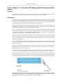
Cover image: A single sideband spectrum covering the whole of one subband
of HIFI towards the Orion nebula, superimposed on a Spitzer Space Telescope
colour composite of the region from IRAC and MIPS images (Credit: NASA).
HIFI Observers' Manual
:
Update for Start of GT2 Observations
Published version 2.3, 31-March-2011
Copyright © 2011
Revision History
Revision version 2.3
APM, DT
Update for changes made for the GT2 call including HSpot 5.3 updates.
Revision version 2.2
APM, DT
Update for changes made for the GT2 call
Revision version 2.1
APM, DT
Update for changes made starting OT1 observations
Revision version 2.0
APM, DT
Update for initial Open Time call (OT1)
Revision version 1.1
APM, DT
Update for initial Open Time Key Projects
Revision version 1.0
Initial version
APM, DT
Table of Contents
1. The HIFI Instrument Observer's Manual ........................................................................ 1
1.1. Purpose of this Document ................................................................................ 1
1.2. Preparing HIFI for Operations ........................................................................... 1
1.3. Acknowledgements ......................................................................................... 2
2. HIFI Instrument Description ........................................................................................ 3
2.1. Instrument and Concept ................................................................................... 3
2.1.1. What is HIFI? ...................................................................................... 3
2.1.2. How Does HIFI Work? ......................................................................... 3
2.2. Instrument Configuration .................................................................................. 5
2.3. HIFI Focal Plane Unit ..................................................................................... 6
2.3.1. The Common Optics Assembly ............................................................... 7
2.3.2. The Beam Combiner Assembly (Diplexer Unit) ......................................... 8
2.3.3. HIFI Mixers ........................................................................................ 9
2.3.4. The Focal Plane Chopper ..................................................................... 10
2.3.5. The Calibration Source Assembly .......................................................... 11
2.4. The HIFI Signal Chain ................................................................................... 11
2.5. HIFI Spectrometers ....................................................................................... 12
2.5.1. The Wide Band Spectrometer (WBS) ..................................................... 12
2.5.2. The High Resolution Spectrometer (HRS) ............................................... 13
3. HIFI Scientific Capabilities and Performance ................................................................ 15
3.1. What Science Is Possible With HIFI? ............................................................... 15
3.1.1. HIFI's Scientific Objectives .................................................................. 15
3.2. Primary Instrument Characteristics ................................................................... 16
3.3. General Instrument Description ........................................................................ 17
3.4. Available Spectrometer Setups ....................................................................... 18
3.4.1. Wide Band Spectrometers (WBSs) ......................................................... 18
3.4.2. High Resolution Spectrometers (HRSs) ................................................... 18
3.5. Mixer Performance ........................................................................................ 19
3.5.1. System Temperatures ........................................................................... 19
3.5.2. Tuning Ranges ................................................................................... 20
3.5.3. Sensitivity Variations Across the IF Band ................................................ 23
3.5.4. Overall Noise Performance ................................................................... 24
3.5.5. Mixer Stabilities ................................................................................. 25
4. Observing with HIFI ................................................................................................ 27
4.1. Introduction .................................................................................................. 27
4.2. The HIFI Observing Modes ............................................................................ 27
4.2.1. Modes of the Single Point AOT I .......................................................... 28
4.2.2. Modes of the Mapping AOT II .............................................................. 36
4.2.3. Modes of the Spectral Scan AOT III ...................................................... 41
4.3. Standing Wave Residuals after Calibration (Pipeline Level 2) ................................ 44
4.3.1. Bands 1-5 (SIS mixers) ........................................................................ 44
4.3.2. Position Switch, Frequency Switch and Load Chop modes .......................... 46
4.4. Bands 6-7 (HEB mixers) ................................................................................ 47
4.4.1. DBS Modes ....................................................................................... 47
4.4.2. Position Switch, Frequency Switch and Load Chop Modes .......................... 48
4.5. "Grouping" or "Clustering" of Observations ....................................................... 48
4.6. Solar System Target Modes ............................................................................ 48
5. HIFI Calibration ...................................................................................................... 49
5.1. Introduction: ................................................................................................. 49
5.2. The Intensity Calibration of HIFI ..................................................................... 49
5.2.1. Context ............................................................................................. 49
5.3. The HIFI Calibration Scheme .......................................................................... 49
5.3.1. Internal Load Calibrations .................................................................... 49
5.3.2. OFF calibration .................................................................................. 51
5.3.3. Differencing observations: .................................................................... 52
iv
HIFI Observers' Manual
5.3.4. Non-linearity: ..................................................................................... 52
5.3.5. Blank-sky contribution: ........................................................................ 52
5.3.6. Conversion between Antenna Temperature and Janskys: ............................. 52
5.4. The Frequency Calibration of HIFI: .................................................................. 52
5.4.1. Context: ............................................................................................ 53
5.4.2. Frequency accuracy: ............................................................................ 53
5.4.3. Determination of Frequency Calibration: ................................................. 53
5.4.4. Frequency resolution: .......................................................................... 53
5.4.5. Frequency and Velocity Verifications ..................................................... 54
5.4.6. Spurious Responses in HIFI .................................................................. 55
5.5. The Spatial Response Calibration of HIFI: ......................................................... 59
5.5.1. Context: ............................................................................................ 59
5.5.2. Beam Characteristics ........................................................................... 59
5.5.3. Chopper Calibration ............................................................................ 67
5.6. Mixer Side-band Ratio ................................................................................... 68
5.6.1. IF Spectrum Repeatability (Sideband Line Ratios) ..................................... 69
5.7. Summary: overall calibration of HIFI and error budget: ........................................ 71
5.7.1. Strategy summary: .............................................................................. 71
5.7.2. Error budget ...................................................................................... 71
6. Using HSpot to Create HIFI Observations ................................................................... 73
6.1. Overview .................................................................................................... 73
6.2. HSpot Components for Setting Up a HIFI Observation ......................................... 73
6.2.1. Working with A HIFI Pointed or Mapping Observation Template ................. 73
6.2.2. HIFI Spectral Scan AOT ...................................................................... 81
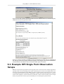
6.3. Example HIFI Single Point Observation Setups .................................................. 84
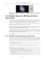
6.3.1. Example 1: Observing the [CII] line using Frequency Switch in a photodissociation region ........................................................................................... 85
6.3.2. Example 2: A Dual Beam Switch (DBS) mode AGB Observation ................. 91
6.4. Example Setup of a HIFI Mapping AOR ........................................................... 96
6.4.1. Example 3: Scan Mapping of the Spectral Lines CO(7-6) and CI(2-1) in the
Centre of M51 . .......................................................................................... 96
6.5. Example Setup of a HIFI Spectral Scan Observation .......................................... 100
6.5.1. Example 4: Spectral Survey of a Hot Core. ............................................ 100
7. Pipeline and Data Products Description ..................................................................... 103
7.1. Data to be Passed on to the User .................................................................... 103
7.2. Additional Observatory Meta Data .................................................................. 103
7.3. Example HIFI data products .......................................................................... 103
7.3.1. Level 0 products ............................................................................... 103
7.3.2. Level 1 products ............................................................................... 104
7.4. Pipeline Processing ...................................................................................... 105
7.4.1. WBS Pipeline Processing Steps ........................................................... 105
7.4.2. HRS Pipeline Processing Steps ............................................................ 106
7.5. Deconvolution Processing of Spectral Scan Data ............................................... 106
7.5.1. Solving the Deconvolution Problem ...................................................... 107
8. References: ........................................................................................................... 109
A. Change Log ......................................................................................................... 110
A.1. ................................................................................................................ 110
v
Chapter 1. The HIFI Instrument
Observer's Manual
1.1. Purpose of this Document
The HIFI (Heterodyne Instrument for the Far Infrared) observer's manual is intended to assist in using
the HIFI instrument on board ESA's Herschel Space Observatory. Documents on the detailed documents on design and operations are available from the Herschel Science Centre (HSC) and the HIFI
Instrument Control Centre at SRON, Groningen, The Netherlands (HIFI ICC -- who are responsible
for the safety and calibration of HIFI during operations).
Help and information on HIFI can be obtained by contacting the Herschel Science Centre at the following web address:
http://herschel.esac.esa.int
Follow the link on the page to the "Helpdesk" for problem enquiries.
This document contains overview information on instrument concept and design, its scientific performance and calibration. It also contains all user-relevant information on observing modes and Astronomical Observing Templates (AOTs) Examples of AOTs for HIFI are presented with their usage.
HIFI data from the Herschel Space Observatory are automatically processed at the HSC after the data
is received from the spacecraft. The standard processing - pipeline - is described here together with
a description of the data products. Both the raw and pipeline processed data are made available to
the user.
Finally, a brief mention is made of software tools that have been more specifically provided for the
kinds of sophisticated analysis that is likely to be needed for HIFI data reduction. These will available to the user through the Herschel Common Science System, which will be made available by the
Herschel Science Centre. It should be noted that all pipeline software modules are available to users
via installation of the Herschel Common Science System. Reprocessing of data can therefore be performed with pipeline, or adapted pipeline, scripts by users on their own workstations.
1.2. Preparing HIFI for Operations
In August 2009, a sequence of events triggered by a corruption of on-board memory lead to the loss
of the prime side electronics chain of HIFI. Since then, a significant effort has been made that has
enabled a full recovery of the instrument using its redundant side electronics.
The special circumstances of HIFI's switch to redundant side operations, and resuming with a compressed Performance Verification phase and accelerated Observing Mode release, has involved the
support of many others, together with the HIFI Calibration Scientists and Instrument Engineers. This
includes KP team apprentices who have been variously present at the HIFI ICC in the Fall of 2009
and during the performance verification phase starting end-January 2010, and also the HIFI software
development team who have been available at all times. AOT test planning has been done in consultation with the KP PIs coordinated by X. Tielens, Instrument P.I. F. Helmich, Project Manager P.
Roelfsema, and with the Mission Scientist J. Cernicharo. These persons should be acknowledged, as
having directly supported the flight qualification of HIFI as a science instrument.
AOT/Uplink Engineering Team: P. Morris (Caltech), M. Olberg (SRON/Chalmers), V. Ossenkopf
(U. Köln), C. Risacher (SRON), D. Teyssier (HSC/ESA).
Instrument Engineers and System Architects: P. Dieleman (SRON), K. Edwards (SRON), W. Jellema (SRON), A. de Jonge (SRON), W. Laauwen (SRON), J. Pearson (JPL).
1
The HIFI Instrument Observer's Manual
HIFI Calibration Scientists: I. Avruch (Kapteyn/SRON), A. Boogert (Caltech), C. Borys (Caltech),
J. Braine (U. Bordeaux), F. Herpin (U. Bordeaux), R. Higgins (U. Maynooth), S. Lord (Caltech), A.
Marston (HSC/ESA) C. McCoey (U. Waterloo), R. Moreno (Obs. Paris), M. Rengel (MPS)
HIFI Software Development Team: R. Assendorp (SRON), B. Delforge (SRON), A. Hoac (Caltech), D. Kester (SRON), A. Lorenzani (Obs. Acetri), M. Melchior (U. Appl. Sci. NW Switzerland),
W. Salomons (SRON), B. Thomas (SRON), E. Sanchez (CSIC), R. Shipman (SRON), Y. Poelman
(SRON), J. Xie (Caltech), P. Zaal (SRON)
HIFI KP student/postdoc visitors: E. DeBeck (U. Leuven), T. Bell (Caltech), N. Crockett (U. Michigan), P. Bjerkeli (Chalmers), P. Hily-Blant (Obs. Grenoble), M. Kama (U. Amsterdam), T. Kaminski
(CAMK), B. Larsson (Obs. Stockholm), B. Lefloch (Obs. Grenoble), R. Lombaert (U. Leuven), M.
de Luca (Obs. Paris), Z. Makai (U. Köln), M. Marseille (SRON), Z. Nagy (Kapteyn), Y. Okada (U.
Köln), S. Pacheco (Obs. Grenoble), D. Rabois (U. Toulouse), Frank Schlöder (U. Köln), S. Wang (U.
Michigan), M. van der Wiel (Kapteyn/SRON), M. Yabaki (U. Köln), U. Yildiz (U. Leiden)
HIFI KP PI Representatives to the ICC/AOT Team: E. Caux (U. Toulouse), E. van Dishoek (U.
Leiden), M. Gerin (Obs. Grenoble)
1.3. Acknowledgements
The HIFI instrument is the result of many years of work by a large group of dedicated people. It is
their efforts that have made it possible to create such a powerful heterodyne instrument for use in the
Herschel Space Observatory. We would first like to acknowledge their work.
The manual itself included help and inputs from a number of people. Particular help and contributions
to this manual have come from
• Anthony Marston (ESAC, editor), 31 March 2011.
• David Teyssier (ESAC)
• Patrick Morris (NHSC)
• Michael Olberg (Onsala)
• Volker Ossenkopf (U. Köln)
2
Chapter 2. HIFI Instrument
Description
2.1. Instrument and Concept
2.1.1. What is HIFI?
HIFI is the Heterodyne Instrument for the Far Infrared. It is designed to provide spectroscopy at high to
very high resolution over a frequency range of approximately 480-1250 and 1410-1910 GHz (625-240
and 213-157 microns). This frequency range is covered by 7 "mixer" bands, with dual horizontal and
vertical polarizations, which can be used one pair at a time (see Table 3.1 for detailed specification).
The mixers act as detectors that feed either, or both, the two spectrometers on HIFI. An instantaneous
frequency coverage of 2.4GHz is provided with the high frequency band 6 and 7 mixers, while for
bands 1 to 5 a frequency range of 4GHz is covered. The data is obtained as dual sideband data which
means that each channel of the spectrometers reacts to two frequencies (separated by 4.8 to 16 GHz)
of radiation at the same time (see Section 2.1.2 and Section 3.1). For many situations, this overlapping of frequencies is not a major problem and science signals are clearly distinguishable. However,
particularly for complex sources containing a high density of emission/absorption lines, this can lead
to problems with data interpretation. Deconvolution is therefore necessary for the data to create single sideband data. This is especially important for spectral scans covering large frequency ranges on
sources with many lines (see Chapter 6).
There are four spectrometers on board HIFI, two Wide-Band Acousto-Optical Spectrometers (WBS)
and two High Resolution Autocorrelation Spectrometers (HRS). One of each spectrometer type is
available for each polarization. They can be used either individually or in parallel. The Wide-Band
Spectrometers cover the full intermediate frequency bandwidth of 2.4GHz in the highest frequency
bands (bands 6 and 7) and 4GHz in all other bands. The High Resolution Spectrometers have variable
resolution with subbands sampling up to half the 4GHz intermediate frequency range. Subbands have
the flexibility of being placed anywhere within the 4GHz range.
2.1.2. How Does HIFI Work?
Sub-mm continuum radiation is best detected with bolometers, which act like thermometers, measuring the heat coming in and translating it to integrated intensities. Line radiation is much more difficult
to detect. There are no amplifiers available to amplify the weak sky signals at sub-millimeter wavelengths. For lower frequencies there are, however, good amplifiers available, which can be small, low
in energy consumption and weight. These are thus very suitable for a space observatory.
2.1.2.1. The Mixers
The solution is thus to bring the signal down in frequency, without losing its information content. This
is accomplished, through heterodyne techniques in which the sky signal is mixed with another signal
(Local Oscillator) very close to the frequency of interest. In performing such mixing of signals, the
resulting signal is of much lower frequency, while still having all the spectral detail of the original
sky-signal. Modern mixing devices such as SIS (semiconductor-insulator-semiconductor) mixers or
hot electron bolometer (HEB) mixers, not only perform the mixing but can also amplify the signal,
making them eminently suitable for instruments like HIFI.
Mixing: The mixers used by HIFI are at superconducting temperatures (the HEBs are on the border
of normal and superconducting). They are non-linear devices in that the current out is not directly
proportional to the voltage across them -- in fact their current-voltage curves have similarities to those
of diodes. This allows amplification of the mixed signals of the incoming radiation and an on-board
local oscillator. In particular, the "beat" frequency ( | fs - fLO | ) between each of the incoming source
frequencies, fs, and the single Local Oscillator frequency, fLO.
3
HIFI Instrument Description
Intermediate Frequency: The "beat" frequencies produce the so-called Intermediate Frequency (IF) of
the instrument. Further amplification is made of these intermediate frequencies and, for HIFI, filtering
allows the detection of IFs of 4 to 8GHz which is done in the HIFI spectrometers.
2.1.2.2. Double Sideband Data
In creating the intermediate frequency it should be noted that a given IF value (e.g., 5GHz) can be
obtained from a source frequency that is either 5GHz higher or 5GHz lower than the local oscillator
frequency. If we consider this for a range of incoming frequencies we can see that our spectrometer
measures two superimposed portions of an object's spectrum.
• The portion of the source spectrum 4 to 8GHz above the LO frequency. This will be in ascending
frequency order from fLO+4GHz to fLO+8GHz. This is the upper sideband (USB).
• The portion of the source spectrum 4 to 8GHz below the LO frequency. This will be in descending
frequency order from fLO-4GHz to fLO-8GHz. This is the lower sideband (LSB).
This superposition is illustrated in Figure 2.1.
Figure 2.1. Superposition of upper (red in double sideband view) and lower (blue in double sideband view)
sideband spectra in a portion of a single DSB spectrum crudely based on Orion cloud spectra taken at
807.0GHz.
Figure 2.2. Superposition of two separate DSB spectra in blue and red taken at 807.0 and 807.13 GHz
respectively. Note how the largest line from the lower sideband goes up in the IF band frequency when
the LO frequency is increased (compare with previous figure), while the other two lines from the upper
sideband go in the opposite direction. In all cases the frequency shift is 0.13GHZ, the same as the LO
frequency change between the two observations.
4
HIFI Instrument Description
2.1.2.3. Consequences of Double Sideband (DSB) Data
For a number of regions where a single strong line of known frequency is the subject of study, knowing
whether it is in the upper or lower sideband frequency range is easy to determine - and so it is easy
to assign the correct frequency to the spectrum scale.
Small LO shifts: However, for cases where it is not known a priori which spectral lines are in which
sideband the simplest way to determine this is by shifting the LO frequency. An increase in LO frequency will lead to USB features moving to lower IF frequencies and LSB features moving to higher IF
frequencies (see Figure 2.2). It then becomes clear which sideband (and frequency) the features are in.
Deconvolution: Even the above technique becomes impossible for regions where there is a high density of spectral features. In such cases, the chances become quite high that USB features and LSB
features will overlap. And the shifting of the LO may only lead to other feature overlaps. For this case
deconvolution techniques have been devised (see Chapter 7). These allow large regions of frequency
space to be sampled by many positionings of the LO frequency. A reconstruction of the spectrum
(single sideband, SSB) can then be made.
2.1.2.4. The HIFI Flux Units: Antenna Temperature
Sub-mm astronomy derives many of its units from radio astronomy. The standard unit for measuring
the power received is antenna temperature, TA, which is defined by:
kTA = power received per unit frequency
If the intensity is constant across the whole beam then the antenna temperature is equivalent to the
brightness temperature (the temperature a blackbody needs to be in order to see the observed intensity
at a given frequency).
This is a particularly convenient scale to use since flux calibration is made by comparison of the source
measurement with measurements of hot and cold blackbody loads internal to HIFI.
However, sources do not usually fill any of the HIFI beams and a correction, usually in the form of an
aperture efficiency, is needed. For more details on the calibration procedure see Chapter 5.
The main noise contribution for measurements is from to the instrument itself. This noise level is
referred to as the system temperature, Tsys
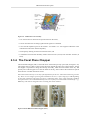
2.2. Instrument Configuration
Referring to Figure 2.3, HIFI has five (hardware) sub-systems: the Local Oscillator and Focal Plane
Sub- Systems; the Wide-Band and High-Resolution Spectrometers; and the Instrument Control Unit.
Within the Local Oscillator Sub-System, a tuneable, spectrally pure 24-36 GHz signal is generated
in the Local Oscillator Source Unit. This signal is then frequency-multiplied (upconverted) to 71-106
GHz, amplified, and further frequency-multiplied, by different factors for each of the LO chains, to
the desired RF frequency in the Local Oscillator Unit. The result is a spectrally pure LO signal with
a tuneable frequency and power level.
Fourteen multiplier chains cover 480-1910 GHz (625 - 157 microns), with two chains for each of
the seven Focal Plane Unit mixer channels. The chain feeding the lower frequencies of the band is
labelled "a" and for the higher frequencies is labelled "b" (leading to the naming of mixer bands as
1a, 1b, 2a etc.).
5
HIFI Instrument Description
Figure 2.3. General HIFI component diagram.
The local oscillator beams are fed into the Focal Plane Unit through 7 windows in the Herschel cryostat.
Within the Focal Plane Unit, the astronomical signal from the telescope is split into 7 beams. Each of
these signal beams is combined with its corresponding LO beam, and then split into 2 linearly polarized
beams that are focused into 2 mixer units. Each mixer unit generates an intermediate frequency (IF)
signal that is amplified prior to leaving the Focal Plane Unit.
The IF output signals from the Focal Plane Unit can be coupled into two IF spectrometers: the WideBand Spectrometer, a four-channel (subband) acousto-optical spectrometer (AOS) that samples the
4-8 GHz band at 1 MHz resolution; and the High-Resolution Spectrometer, a high-speed digital autocorrelator (ACS) that samples narrower portions of the IF band at resolutions up to 140 kHz.
Each of the spectrometers includes a warm control electronics unit. These four control units are, in
turn, commanded by a single Instrument Control Unit (ICU), which also interfaces with the satellite's
command and control system.
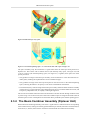
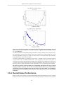
2.3. HIFI Focal Plane Unit
The HIFI Focal Plane Sub-System consists of three hardware units: the Focal Plane Unit (FPU, see
[1]), which is located on the optical bench in the Herschel cryostat and depicted in Figure 2.4 and
Figure 2.5; the Up-converter and 3-dB Coupler (described in Section 2.4) are contained in the satellite's
service module -- see the Observatory handbook for details on the service module; and the Focal Plane
Control Unit (FCU), also contained in the satellite's service module). Additionally, the critical signal
chain elements that together define the instrument's sensitivity (the mixers, isolators in bands 1 to 5,
and amplifiers, plus the IF up-converter used in Bands 6 and 7) together form the HIFI Signal Chain.
6
HIFI Instrument Description
Figure 2.4. HIFI Focal Plane Unit (FPU).
In practice, the HIFI signal chain is a virtual unit, since its elements are physically distributed throughout the FPU. The complexity of the FPU has necessitated a modular design in which the Focal Plane
Unit is divided into six major assemblies: the Common Optics Assembly; the Diplexer (beam combiner) Assembly; the Mixer Sub-Assemblies (of which there are 14); the second-stage IF amplifier
box; the Focal Plane Chopper; and the Calibration Source Assembly (see Figure 2.4).
Figure 2.5. Back side of the HIFI FPU.
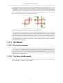
2.3.1. The Common Optics Assembly
The Common Optics Assembly, forms the basis of the FPU structure, and mounts directly on the
Herschel optical bench.
7
HIFI Instrument Description
Figure 2.6. HIFI telescope relay optics.
Figure 2.7. The channel splitting optics -- as seen from the side with respect to Figure 2.6.
The optics assembly relay the instrument's 7 signal beams from the telescope's focal plane into a
diplexer box. This is done with 6 common mirrors (the telescope relay optics, see Figure 2.6) and
7 sets of 3 mirrors (the channel-splitting optics, see Figure 2.7). Together, these optics have three
primary functions:
• They produce an image of the telescope secondary on the fourth mirror in the chain after the secondary (M6), enabling the implementation of a Focal Plane Chopper.
• They produce an image of the telescope focal plane on the first mirrors in the Channel-Splitting
Optics, allowing the beams to be split by seven mirrors with different orientations.
• In each channel, they create an image of the telescope secondary within the beam combiner assembly
(see Section 2.3.2). This image has a large Gaussian beam waist, to minimize diffraction losses, and
a frequency independent size, to simplify visible-light alignment.
The seven local oscillator beams from the Local Oscillator Unit enter the FPU through windows in the
cryostat. Using 7 sets of five mirrors, the Cold Local Oscillator Optics re-image the LO beam waists at
the FPU input to waists in the diplexer box that match those produced by the channel-splitting optics.
2.3.2. The Beam Combiner Assembly (Diplexer Unit)
Within the beam combining assembly, each of the 7 signal beams is combined with its corresponding
local oscillator beam, creating two linearly polarized beams per channel (referred to as Horizontal, H,
and Vertical, V, beams). Each of these 14 beams is then directed into a Mixer Sub-Assembly.
8
HIFI Instrument Description
At low frequencies, where significant LO powers are available, the combining is done with polarizing
beamsplitters. As seen in Figure 2.8, one beamsplitter is placed at the intersection of the LO and
signal beams, creating two mixed beams (one contains the horizontally polarized signal beam and the
vertically polarized LO beam, while the second contains the inverse). Each of the mixed beams then
hits a second beamsplitter, which is oriented to reflect 90% of the signal power and 10% of the LO
power (the remaining power is absorbed in a beam-dump).
Figure 2.8. Beamsplitter and diplexer mixing with sample diplexer unit.
At high frequencies, where LO power is scarcer, a Martin-Puplett diplexer is used for LO injection
(see Figure 2.8). As in the beamsplitter channels, the first beamsplitter creates two beams containing
LO and signal power in orthogonal polarizations. However, in this case, the second beamsplitter is
replaced with a polarizing Michelson interferometer that rotates the LO beam polarization relative to
that of the signal beam, creating a linearly polarized output. In this manner, the coupling of both the
LO and signal powers to the mixers is high (95%, or better), although diplexer scanning mechanisms
are needed for frequency tuning.
2.3.3. HIFI Mixers
2.3.3.1. Device Technologies
The mixers at the heart of the Focal Plane Unit largely determine the instrument's sensitivity. For this
reason, the mixer technologies used in each band have been selected to yield the best possible sensitivity. In particular, a range of Superconductor-Insulator-Superconductor (SIS) mixer technologies are
being used in the lowest 5 frequency bands (covering 480-1250 GHz; see Refs [2], [3], [4] and [5]),
while the top two bands (covering 1410-1910 GHz; see Refs [6], and [7]) incorporate Hot Electron
Bolometer mixers (HEB mixers).
2.3.3.2. The Mixer Sub-Assembly
Each of the 14 linearly polarized outputs from the diplexer/beam combiner box enters a Mixer SubAssembly (MSA -- see Figure 2.9) that includes:
9
HIFI Instrument Description
Figure 2.9. A HIFI mixer sub-assembly.
• a set of three mirrors that focus the optical beam into the mixer;
• a mixer unit where the incoming signal and LO signal are combined;
• a low-noise IF amplifier (plus two IF isolators - for bands 1 to 5 - that suppress reflections in the
cable between the mixer and the amplifier);
• low-frequency filtering for the mixers DC bias lines; and
• a mechanical structure that thermally isolates the mixer unit (at 2 K) from the FPU structure (at
10 K).
2.3.4. The Focal Plane Chopper
The Focal Plane Chopper (FPC) is the sixth mirror of the telescope relay optics (M6, see Figure 2.10).
The chopper mirror is able to rotate (in one direction) around the centre of its optical surface. Tilting
the chopper is equivalent to tilting the telescope secondary, which moves the beam on the sky. The
primary uses of the chopper are to steer the beam on the sky, and to redirect the instrument's optical
beam into the on-board calibration sources.
The beam switch on the sky is currently a fixed parameter for the user. The beam switch being 3' on the
sky. There are two chopper speed regimes available to the user, a "fast" chop (up to 4Hz depending
on the goal resolution, being faster for larger resolutions) and a "slow" chop (typically 0.125Hz if
all 4 spectrometers are used simultaneously, but twice as fast if two backends are switched off -- e.g.,
WBS only). The FPC is designed to have a settling time under 20msecs.
Figure 2.10. The HIFI Focal Plane Chopper (FPC).
10
HIFI Instrument Description
2.3.5. The Calibration Source Assembly
Mounted on the side of the Common Optics Assembly, the Calibration Source Assembly includes two
blackbody signal loads that are used to calibrate the instrument's sensitivity (the first is an absorber
at the FPU temperature around 10K, while the second is a lightweight blackbody cavity that can be
heated to 100K), plus mirrors that focus the FPU's optical beam into the loads. Temperature sensors
are available to read out the actual temperature of both calibration loads. The HIFI optical beam is
steered towards the calibration sources by the use of extreme positions of the Focal Plane Chopper.
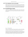
2.4. The HIFI Signal Chain
As seen in Figure 2.11, the HIFI Signal Chain includes the 14 Mixer Units, the First- and Second-Stage
Amplifiers (in the FPU), the Upconverter and 3-dB Coupler (which are located in the satellite's service
module), and the Isolators that are used to suppress reflections between the Mixer Units and the FirstStage Amplifiers.
Figure 2.11. The HIFI signal chain.
In Bands 1 to 5, each Signal Chain consists of a mixer, followed by two isolators, and two amplifiers.
For each polarization, the outputs of these 5 independent chains are combined, so that only two cables
are needed to carry the IF outputs from these 10 channels of the FPU to the service module.
The situation in Bands 6 and 7 is similar, except that isolators are not used (because they are not
available for the 2.4-4.8 GHz IF band that is needed for the HEB mixers). Thus, the second pair of IF
output cables from the FPU includes the combined outputs of the two polarizations of Band 6 and 7.
The other difference in the Band 6/7 Signal Chain is that an IF Up-converter is needed to transform
the 2.4-4.8 GHz output of the FPU to 8-5.6 GHz, for compatibility with the spectrometers.
11
HIFI Instrument Description
Within the "IF Up-converter" (in the service module), a 3-dB Coupler is also used to combine the
Bands 1-5 and 6-7 outputs, so that each "polarization" of the Wide-Band and High-Resolution Spectrometers is connected to all 7 bands by a single input cable (although a signal is only received from
the active band).
2.5. HIFI Spectrometers
The HIFI instrument provides an IF bandwidth of 4GHz in all bands except for band 6 and band 7
(1408-1908GHz) where only 2.4GHz bandwidth is available. To sample this bandwidth, HIFI has
4 spectrometers. A Wide Band Spectrometer (WBS) and High Resolution Spectrometer (HRS) are
available for each of the polarizations. All spectrometers can be used in parallel, although at fast data
rates it is necessary to reduce how much is readout and stored since, at the highest data rates, the
spectrometers provide data at a rate that is higher than the bandwidth available to HIFI on board the
spacecraft.
The WBS is an Acousto-Optical Spectrometer (AOS) able to cover the full IF range available (4GHz)
at a single resolution (1.1MHz). The HRS is an Auto-Correlator System (ACS) with several possible
resolutions from 0.125 to 1.00MHz but with a variable bandwidth that can cover only portions of
the available IF range. The HRS can be split up to allow the sampling of more than one part of the
available IF range.
In the following two subsections, we describe the main workings of the two spectrometer types available to HIFI.
2.5.1. The Wide Band Spectrometer (WBS)
The WBS is based on two (vertical and horizontal polarization) four channel Acousto-Optical Spectrometers (AOS; see [8]) and includes IF processing and data acquisition. To cover the 2 x 4-8 GHz (2
x 2.4-4.8GHz for bands 6 and 7) input signals from the FPU, two complete spectrometers (horizontal
+ vertical polarization) are used. For redundancy reasons both spectrometers are fully independent.
Each spectrometer receives a pre-amplified and filtered IF-signal (4-8 GHz). After further amplification in the WBS electronics, the signal is split into four channels which provide the input frequency
bands for the WBS optics (4 x 1.55-2.65 GHz; IF1 to IF4). The signal is further amplified and equalised
(using variable attenuators), to compensate for non-uniform gain of the system, before being sent to
two Bragg cells in the optics module of the WBS.
The other necessary input is to provide a frequency reference signal for the frequency calibration
of WBS spectra. This is done using a 10 MHz reference signal from the Local Oscillator Source
Unit (LSU), is fed into the WBS to provide a "comb" signal. The comb signal in the WBS, with
regular stable 100 MHz line spacing, can be connected for frequency calibration purposes or it can
be disabled to provide a zero level measurement of the AOSs. The zero allows allows more precise
system temperature measurements to be made.
In the optics section of the WBS, the pre-processed IF-signal from the mixers is analysed using the
acousto-optic technique. The IF-signal is fed into a Bragg cell via a transducer. The IF-signal then
generates an acoustic wave pattern in the Bragg cell crystal. A laser beam which enters the Bragg cell
is diffracted according to the acoustic wave pattern in the Bragg cell crystal. The diffracted laser light
is afterwards detected by four linear CCDs with 2048 pixels each and each covering approximately
1GHz bandwidth. Four vertically aligned Bragg cells and CCD chains are necessary to cover the full
4 GHz IF bandwidth of HIFI.
The WBE electronic section has 4 analogue line receivers for the 4 CCD video signals. These signals
are fed to 14 Bit analogue to digital converter with a conversion speed corresponding to less than 3
ms. The relatively high number of ADC-Bit is meant to keep differential non-linearity effects to a very
low level. Overall non-linearity in the WBS is very low, less than 1%..
Continuous data taking is possible without dead time during data transfer, as long as the integration
time is above 1 sec -- which is true for all standard operating modes of HIFI.
12
HIFI Instrument Description
Every 10 ms the collected photoelectrons in the CCD photodiodes are shifted into a register and
clocked out serially. After integration completion, the data can be transferred while a new integration
is started. Data is transmitted to the Instrument Control Unit (ICU) with 16 or 24 Bits through a serial
interface with 250 kHz clock rate which is synchronous with the CCD read-out clock. Housekeeping
data is provided through the same interface. A second serial interface is used for the command interface.
2.5.2. The High Resolution Spectrometer (HRS)
With the HRS, high resolution spectra are available from any part of the input IF bandwidth (4GHz, or
2.4GHz in band 6 or 7). The HRS is an Auto-Correlator Spectrometer (ACS) that can process simultaneously the 2 signals coming from each polarization of the FPU. It is composed of two identical units:
HRS-H and HRS-V. Each of which includes an IF processor, a Digital Autocorrelator Spectrometer
(ACS) and associated digital electronics, plus a DC/DC converter (not discussed here). The HRS provides capability to analyse 4 subbands per polarization, placed anywhere in the 2.4 or 4 GHz input
bands coming from the Focal Plane Unit (FPU). The two units of the HRS can be used to process
the same 4 sub-band frequency ranges in each of the two polarizations provided by the FPU, thereby
reducing the integration time and providing redundancy. Both units of the HRS operate at the same
time and it is possible to look at either IF with each of the HRS spectrometers.
2.5.2.1. Overview of the HRS Subsystem
In each HRS unit the ACS processes the signals coming from its associated IF (see [9]). Each 230
MHz band width input is digitized by a 2 bit / 3 level analogue to digital converter clocked at 490
MHz. The digital signals are analysed with a total of 4080 autocorrelation channels. It is possible to
configure the HRS to provide 4 standard modes of operation as given in Table 3.2. For example, in
its nominal resolution the HRS proves two sub-band spectra each of which have a bandwidth of 230
MHz, each of which is covered by 2040 channels and has a spectral resolution of 250kHz.
It is possible to set each sub-band frequency independently anywhere in the 4 GHz IF band range.
Two buffers are used, with selection synchronised with the chopper position by the ICU. The HRS
has a maximum chopping frequency of 5 Hz. The data can be accumulated in each buffer up to a
maximum of 1.95 seconds. The data readout duration is about 42 ms. Data can be read out from one
buffer while data accumulation occurs on the other.
2.5.2.2. Modes of HRS Operation -- Wide Band Mode
In the wide band mode all 4080 correlation channels of the ACS are used to analyse the 8 input signals.
As the input signals are adjacent two by two, 4 sub-bands of each of 460 MHz bandwidth can be
analysed in this mode. The four sub-bands can be independently placed anywhere in the IF bandwidth
range. It is possible to analyse almost the whole 4 GHz input IF bandwidth by selecting the same
polarization in the two HRS units and by setting the lose to have adjacent sub-bands.
In this mode, with a Hanning windowing of the correlation function, the spectral resolution is 1000
kHz. The total band-width per HRS unit is 2 GHz.
In each correlator ASIC one channel is dedicated to compute the analogue signal offset.
2.5.2.3. Modes of HRS Operation -- Low Resolution Mode
In the low resolution mode the 4080 correlation channels are used to analyse 4 of the 8 input signals
of 230 MHz band width each. The four sub-bands can be independently placed anywhere in the IF
bandwidth.
In this mode, with a Hanning windowing of the correlation function, the spectral resolution is 500
kHz. The total band-width per HRS unit is 1 GHz.
In each correlator ASIC one channel is dedicated to compute the analogue signal offset.
13
HIFI Instrument Description
2.5.2.4. Modes of HRS Operation -- Nominal Resolution Mode
In the nominal resolution mode the 4080 correlation channels are used to analyse 2 of the 8 input
signals of 230 MHz band width each. The two sub-bands can be independently placed anywhere in
the IF bandwidth range.
In this mode, with a Hanning windowing of the correlation function, the spectral resolution is 250
kHz. The total band-width per HRS unit is 460 MHz.
In each correlator ASIC one channel is dedicated to compute the analogue signal offset.
2.5.2.5. Modes of HRS Operation -- High Resolution Mode
In the high resolution mode the 4080 correlation channels are used to analyse 1 of the 8 input signals
of 230 MHz band width each. The sub-band can be placed anywhere in the IF bandwidth range.
In this mode, with a Hanning windowing of the correlation function, the spectral resolution is 125
kHz. The total band-width per HRS unit is 230 MHz.
In each correlator ASIC one channel is dedicated to compute the analogue signal offset.
14
Chapter 3. HIFI Scientific Capabilities
and Performance
The HIFI instrument has been designed to provide very high spectral resolution across a large range
of far-infrared and sub-millimetre wavelengths. A large fraction of the frequency range covered by
the instrument can not be observed from the ground.
In this chapter we discuss the range of science capabilities of the instrument.
3.1. What Science Is Possible With HIFI?
HIFI's very high spectral resolution coupled with its ability to observe thousands of molecular, atomic
and ionic lines at sub-millimeter wavelengths make it the instrument of choice to address many of
the key questions in modern astrophysics related to the cyclic interaction of stars and the interstellar
medium. A wide range of chemical and dynamical studies are possible using HIFI. However, the
original set of science objectives for the instrument are given in the following section.
3.1.1. HIFI's Scientific Objectives
At the outset of the mission, the major scientific objectives of the HIFI instrument are:
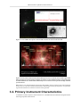
• to probe the physics, kinematics, and energetics of star forming regions through their cooling lines,
including H2O (see Figure 3.1);
• to survey the molecular inventory of the wide variety of regions that participate in the life-cycle
of stars and planets;
• to search for low-lying transitions of complex species (i.e. PAHs) and thus study the origin and
evolution of the molecular universe;
• to determine the out-gassing rate of comets through measurements of H2O and to study the distribution of H2O in the giant planets;
• to measure the mass-loss history of stars which regulates stellar evolution after the main sequence,
and dominates the gas and dust mass balance of the Interstellar Medium (ISM) -- see Figure 3.2;
• to measure the pressure of the interstellar gas throughout the Milky Way and resolve the problem
of the origin of the intense Galactic [CII] 158 micron emission measured by COBE;
• to determine the distribution of the 12C/13C and 14N/15N ratios in the Milky Way and other galaxies (to
constrain the parameters of the Big Bang and explore the nuclear processes that enrich the ISM); and
• to measure the far-infrared line spectra of nearby galaxies as templates for distant, possibly primordial galaxies.
15
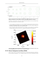
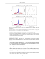
HIFI Scientific Capabilities and Performance
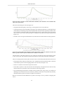
Figure 3.1. One of HIFI's first spectra. The 557 GHz water line as seen in Comet Garradd
Figure 3.2. Early Science Demonstration Phase HIFI spectral scan towards the Orion nebula region. Multiple LO settings were used to obtain a complete spectrum across the available frequency range of the whole
of a HIFI subband. The combined dual sideband spectra were deconvolved to provide the single sideband
spectrum shown.
HIFI achieves very high resolution spectroscopy that enables velocity structures also to be measured.
In this sense it is also an excellent instrument for determining accurate gas dynamics of a particular
region with resolutions of a fraction of a km/s easily possible.
3.2. Primary Instrument Characteristics
To fulfil the scientific objectives noted in Section 3.1, the HIFI instrument has been designed with the
following important characteristics:
16
HIFI Scientific Capabilities and Performance
• complete coverage of 480-1250 and 1410-1910 GHz (625-240 and 213-157 microns), to allow
multiples lines of important molecules, such as H2O, to be sampled, and to allow broad, unbiased
spectral surveys;
• a resolving power of up to 107, corresponding to a velocity resolution up to 0.03 km/s (requiring
a narrow local oscillator line-width and an Intermediate Frequency (IF) spectrometer -- measuring
the frequency difference between signal and local oscillator signals -- with a resolution of up to
125 kHz);
• a receiver sensitivity of 3-4 times the quantum limit, to make maximum use of the limited satellite
lifetime (requiring low-noise mixers and IF amplifiers);
• a large instantaneous band-width (4 GHz in each sideband) to increase spectral survey speeds, to
minimize the risk of spectral coverage gaps, and to observe broad features (requiring mixers, amplifiers, and a spectrometer with 4 GHz of IF bandwidth);
• dual-polarization operation to make maximum use of the energy collected by the HIFI optical beam;
and
• at least 10% calibration accuracy (with a goal of 3%)
NOTES:
1. The time needed to observe a weak spectral line scales inversely with the square of the receiver
noise temperature.
2. The bandwidth is only 2.4 GHz in Bands 6 and 7 (due to a bandwidth limitation in the state-of-theart HEB mixers that are used at these high frequencies).
3. For bands 5, 6 and 7, the receiver temperatures are rather 10-20 times the quantum limit.
3.3. General Instrument Description
The HIFI instrument provides continuous frequency coverage over the range 480-1250 GHz (625-240
microns) in five bands with approximately equal tuning range. An additional pair of bands provide
coverage of the frequency range 1410-1910 GHz (213-157 microns). The instrument operates at only
one local oscillator frequency at a time.
In all mixer bands two independent mixers receive both horizontal and vertical polarizations of the
astronomical signal, although in some cases reduced bandwidth or use of a single polarization is required to stay within the data rate available to the instrument.
The user has the choice of using only a single polarization if he/she chooses.
The first 5 mixer bands use SIS (superconductor-insulator-superconductor) mixers; bands 6 and 7, use
Hot-Electron Bolometers (HEBs).
The instantaneous bandwidth of the instrument will be 4 GHz. The frequency coverage of the instrument is summarised in Table 3.1.
17
HIFI Scientific Capabilities and Performance
Table 3.1. HIFI frequency coverage and band allocation. Note that the values presented are Local Oscillator
frequencies. Each band is further split in two ("a" and "b") due to the use of two Local Oscillator chains
for the lower and upper portions of the frequency range for each band. A further 8GHz is available at each
end of the frequency range due to the frequency placement of the upper and lower sidebands in HIFI in
bands 1 to 5. This is only a further 4.8GHz in bands 6 and 7.
Band
Mixer type
LO
freq.
Lower LO
freq.
Upper Beam
Size
IF Bandwidth
(HPBW)
1
SIS
488.1 GHz
628.4 GHz
39"
4.0 GHz
2
SIS
642.1 GHz
793.9 GHz
30"
4.0 GHz
3
SIS
807.1 GHz
952.9 GHz
25"
4.0 GHz
4
SIS
957.2 GHz
1113.8 GHz
21"
4.0 GHz
5
SIS
1116.2 GHz
1271.8 GHz
19"
4.0 GHz
6+7
HEB
1430.2 GHz
1901.8 GHz
13"
2.4 GHz
3.4. Available Spectrometer Setups
HIFI has four spectrometers, one Wide Band Spectrometer (WBS) and one High Resolution Spectrometer (HRS) per polarization. These may all be used simultaneously. When all spectrometers are
in use frame times are 4 seconds each. Shorter frame times are possible when only one type of spectrometer is used (1 or 2 seconds).
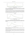
The high resolution spectroscopy modes available with HIFI are most useful for observing faint details and to separate adjacent spectral lines from each other. The contrast between higher and lower
resolution data is illustrated in Figure 3.3 which shows spectra for the Orion-Irc2 region.
Figure 3.3. Example of the use of high resolution spectroscopy in the Orion-Irc2 region.
3.4.1. Wide Band Spectrometers (WBSs)
The Wide Band Spectrometers have a single resolution (1.1MHz) with pixels of width around
0.54MHz (varies slightly across the IF bandwidth). A total contiguous IF bandwidth of 4GHz is covered by 4 linear CCDs that cover 1GHz bandwidth each. Precise frequency calibration is available via
an internal comb generation, supplying a signal providing a regular line spectrum with lines 100MHz
apart. Two buffers are available for source and reference spectra.
3.4.2. High Resolution Spectrometers (HRSs)
The High Resolution Spectrometers have configurations with a variable resolution that is user selectable (see Table 3.2). Between one and four subbands of 230MHz of 460MHz bandwidth can be
18
HIFI Scientific Capabilities and Performance
centred anywhere within the 4GHz intermediate frequency range made available to the spectrometers.
Frequency calibration comes from the internal local oscillator frequency settings for the spectrometer.
Two buffers are available for source and reference spectra.
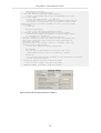
Table 3.2. List of HRS configurations available in each polarization
Mode
Number
of
bands per po- Number
larization
x lags
bandwidth
Spectral resoof Number of off- lution (kHz) - Channel spacset channels
Hanning type ing (kHz)
apodisation-.
High resolution 1 x 230MHz
1 x 4080
16
125
64
Nominal reso2 x 230MHz
lution
2 x 2040
16
250
125
Low resolution 4 x 230MHz
4 x 1020
16
500
250
16
1000
500
Wide resolu- 4 x 460MHz
4 x 510 (x2)
tion (band)
(x2)
3.5. Mixer Performance
Further information beyond what is provided here can be found on the Herschel Science Center's website for the AO release http://herschel.esac.esa.int/AOTsReleaseStatus.shtml. Please see this area for
more detailed information and any updates on HIFI instrument performance and AOTs. The calibration pages will contain up to date calibration information including system temperature vs IF for all
tuned LO frequencies (also see Section 3.5.2).
3.5.1. System Temperatures
Figure 3.4 summarises the current status of measured mixer performance in each of the HIFI mixer
bands. The values shown are the ones currently used in HSpot used in planning HIFI observations.
These values are good for the currently measured "best" polarization for each band. Some variation
in sensitivity does occur across the IF frequency band (see Section 3.5.3) and some deterioration of
sensitivity occurs towards band edges, notably for the situation where diplexers are used for beam
combining (bands 3, 4, 6 and 7).
At present, line selection in HSpot automatically places spectral lines at a good position for sensitivity, avoiding internal spectrometer boundaries (e.g., between 2 CCDs of the WBS spectrometer) and
bandwidth either side of the chosen line.
Observations from both horizontal and vertical polarizations may be combined, but system noise levels
typically vary for each of the bands and a reduction in observation noise by combining polarizations
is slightly less than square root of 2.
Detailed plots of the system sensitivity changes across all the bands are available from the Herschel Science Centre website in the HIFI instrument calibration area of http://herschel.esac.esa.int/
AOTsReleaseStatus.shtml.
19
HIFI Scientific Capabilities and Performance
Figure 3.4. Double sideband system system temperatures of HIFI mixers (bands 1 to 5 are SIS mixers, bands
6 and 7 are HEB mixers), as used in HSpot. System temperatures are based on in-flight measurements
using the internal calibrators of HIFI together with the H and V polarizations of the WBS spectrometer.
The institutions that created the different mixer subbands are indicated.
3.5.2. Tuning Ranges
In addition to certain known impure frequencies (see Section 5.4.6), the various HIFI LO chains have
frequency ranges in which they cannot provide enough output power in order to sufficiently pump the
mixers. The receiver noise temperature is very high in these ranges. Unlike the purity issues, however,
there is little improvement to be expected on the short term so these areas must be considered as
regions of low performance, over the spectral coverage currently achievable by HIFI.
While the border between sensitive and non-sensitive ranges is not abrupt and the noise degradation
is often gradual, the band edges are defined and set in HSpot to avoid frequencies where the mixers
are not even marginally pumped. Between the formal (HSpot) band limits, Users are able to recognize
LO frequencies which offer lower performances from the output of time estimation in HSpot: at the
requested LO frequency (Point and Map AOTs), the noise temperature is quoted in the Message window. The effect of higher noise temperature is to increase the observing time at a fixed noise goal
(entered by the User), or conversely to reduce the S/N ratio at a fixed observing time goal. It is always
worthwhile for the User to attempt to find a setting which minimizes the noise, where some flexibility
is allowed in the IF placement of the spectral line(s) of interest.
Note that system temperatures have been measured to a granularity of ~2 GHz, and therefore only
significant differences may be noticed when changing the LO frequency that switches the target line(s)
from one image band to the other.
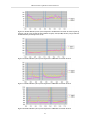
Figure 3.4 illustrates the overall distribution of the receiver noise temperatures as measured in flight.
All temperatures are the median DSB receiver temperatures over the full WBS bandwidth, in K. Frequencies are in GHz. There are two types of poor sensitivity ranges:
More detailed information for each of the bands is provided in Figure 3.5, Figure 3.6, Figure 3.7,
Figure 3.8, Figure 3.9, Figure 3.10, and Figure 3.11.
20
HIFI Scientific Capabilities and Performance
Figure 3.5. Double sideband system system temperatures of HIFI mixers in bands 1a and b. In plots up
to Figure 3.11 the x-axis provides the local oscillator frequency used (in GHz) and the y-axis provides the
double sideband system temperature (in K).
Figure 3.6. Double sideband system system temperatures of HIFI mixers in bands 2a and b.
Figure 3.7. Double sideband system system temperatures of HIFI mixers in bands 3a and b.
Figure 3.8. Double sideband system system temperatures of HIFI mixers in bands 4a and b.
21
HIFI Scientific Capabilities and Performance
Figure 3.9. Double sideband system system temperatures of HIFI mixers in bands 5a and b.
Figure 3.10. Double sideband system system temperatures of HIFI mixers in bands 6a and b.
Figure 3.11. Double sideband system system temperatures of HIFI mixers in bands 7a and b.
• Those with a marginally, but still pumped mixer. They show up as receiver temperatures of the order
of 2-3 times the average temperatures. These frequency areas are considered in the range offered in
HSpot, and will be scanned through during spectral scan measurements, usually with an integration
time doubled compared with other frequencies.
• Those where the mixer cannot be pump at all. Such ranges at band edges have been cut off from
the HSpot front-end frequency ranges so that no time is spent observing at those frequencies. When
those holes occur in the middle of a band, they are still offered to the User, and will be scanned
through during spectral scan, usually with an integration time doubled compared with other frequencies. However, at those frequencies, the data may have to be discarded for an optimum SSB
deconvolution. Only bands 4a, 4b and 6a are concerned by this situation. It should also be noted
that there can be sensitivity issues at the upper end of 7b (above 1898 GHz); despite having enough
LO power the tuning algorithm is not yet fully stable there.
22
HIFI Scientific Capabilities and Performance
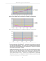
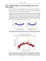
3.5.3. Sensitivity Variations Across the IF Band
The 2.4GHz (in bands 6 and 7) or 4GHz (all other bands) bandwidth of the spectra obtained out of the
instrument are known to have some variations in sensitivity.
Bands using beamsplitters. Here, the sensitivity variations are not particularly large across the band.
This is the case for bands 1, 2 and 5. But IF mismatch can occur at some specific frequencies, resulting
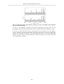
in narrow features of noise excess in the IF (see Figure 3.12).
Figure 3.12. Band 1b showing an IF mismatch at 7000 MHz. It is particularly noticable in the V polarization
at this LO frequency.
Bands using diplexers. In the diplexer bands 3, 4, 6 and 7, a substantial increase in system temperatures
and thus decrease in sensitivity occurs towards the edges of the IF bandpass. For Bands 3 and 4, the
IF bandpass span is 4 GHz (4 - 8 GHz), and the last 500 MHz at either side, between 4.0-4.5 GHz
and between 7.5-8.0 GHz, has a significant increase of baseline noise since the diplexer mechanism
introduces extra losses in these locations. Tsys can increase by up to 50-100% as compared to the
central part of the IF.
The high frequency bands 6 and 7. These bands also have diplexers with the characteristic U-shaped
sensitivity across the IF range. However, the nixer gain dependence over the IF leads to a systematic
rise in system temperatures (reduction in sensitivity) from the lower frequencies of the IF band to the
higher frequencies.
An illustration of the sensitivity change for band 4a is shown in Figure 3.13
23
HIFI Scientific Capabilities and Performance
Figure 3.13. Variation of IF sensitivity at 997.0 GHz in band 4a and 1478.0 GHz in band 6a that shows the
typical variation of system temperature across the IF band for a diplexer subband, including -- in band
6a -- for an HEB mixer.
An additional drawback is degraded stability performance (stronger standing waves and poorer baseline performance). Note that such stability issues can be mitigated by using Fast-DBS, but not the
sensitivity degradation. The option "1 GHz ref" can be used (i.e. un-ticked) to help with the stability
of the degraded part of the IF at band edges.
It is thus a recommendation to avoid placing lines in the last ~500 MHz on either end of the IF in Bands
3 and 4, and in the last ~250 MHz in Bands 6 and 7, when using modes of the Point or Map AOTs. In
cases where two lines are being targeted in the edges of the upper and lower sideband in a single AOR,
it is better to devise separate AORs for each line despite the additional 180 sec slew tax, since time is
not being saved in a single AOR when the noise and standing waves are impeding spectrum quality.
Note that spectral lines selected in HSpot are automatically placed in the best part of the IF
frequency band for sensitivity. The user can override this if he/she chooses (e.g. to allow further
spectral lines to become available in the same spectrum) by use of the slider or by inputting a
specific frequency in the frequency editor table for a given spectrometer (see the user manual
for details).
3.5.4. Overall Noise Performance
HSpot provides noise estimates on a single sideband (SSB) main-beam brightness scale for combined
H and V polarization spectra. Observations carried out during performance verification were analysed
24
HIFI Scientific Capabilities and Performance
in order to verify these predictions, which drive observing time at goal and maximum spectral resolutions entered in HSpot by the User. The 1 GHz reference option has almost always been used in
the noise predictions, which means that the baseline in only one WBS sub-band is considered for stability instead of the full IF, to take standing waves within that 1 GHz window into account. This is
recommended for most observing situations except, when lines are very broad (such as from external
galaxies or fast outflows).
Noise estimates from HSpot 5.0 have been found to be consistent with those actually observed using
the various HIFI observing modes.
3.5.4.1. Noise Performance in Spectral Scans
The noise in the Spectral Scans when measured before sideband deconvolution scales with [2 x redundancy]-1/2, to the single sideband (SSB) noise when the gains are equal (0.5). When the gains deviate
from this value, the deconvolution algorithm should model these as well and the same scaling should
apply. So far there are no indications of a departure away from 0.5.
Analysis of the Spectral Scans taken during performance verification indicate that the deconvolved
SSB root mean square (RMS) noise values are found to be in good agreement, but also sometimes
1.5 to 2 times higher than the HSpot predictions in Bands 1-5. Very preliminary deconvolution results
indicate that the HEB Bands 6 & 7 suggest an even higher SSB RMS noise - between 2-3 times more
than currently predicted by HSpot. Further work is ongoing and updates will be provided to users as
results are obtained.
Observers should keep in mind that the production of good SSB spectra is highly dependent on the
removal all artefacts: standing waves, spurs, and the removal of all continuum baselines (linear or nonlinear) prior to performing the deconvolution reduction step.
Note: When using the DBS reference mode of the spectral scan in bands 6 and 7 users should use the
fast DBS mode rather than normal (slow) chop speed mode.
3.5.5. Mixer Stabilities
Stability measurements have been made at several frequencies for each of the subbands in flight.
Results are now incorporated into the observing sequences produced by HSpot (see Table 3.3).
25
HIFI Scientific Capabilities and Performance
Table 3.3. Allan stability times of the HIFI instrument measured for different noise resolutions and reference bandwidths
Continuum stability time (secs)
Band
Spectroscopic stability time (secs)
Full backend
Full backend
1GHz bandwidth
1a
6.5
3.5
0.8
64.0
42.0
16.0
170.0
120.0
55.0
1b
6.5
3.6
0.8
46.0
30.0
10.0
150.0
99.0
37.0
2a
14.0
8.7
2.2
71.0
48.0
16.0
300.0
220.0
93.0
2b
7.1
3.6
1.0
35.0
19.0
6.2
160.0
88.0
29.0
3a
3.4
2.1
0.7
25.0
14.0
4.8
65.0
40.0
15.0
3b
6.5
5.0
1.5
65.0
50.0
15.0
250.0
200.0
72.0
4a
1.8
1.4
0.5
9.1
7.3
2.6
120.0
98.0
38.0
4b
7.8
3.1
0.6
59.0
26.0
6.5
240.0
120.0
36.0
5a
13.0
4.4
0.9
110.0
45.0
13.0
310.0
160.0
60.0
5b
12.0
4.3
0.9
82.0
39.0
13.0
210.0
120.0
55.0
6a
1.3
0.6
0.2
11.0
4.9
1.7
32.0
15.0
5.4
6b
2.8
0.8
0.2
42.0
15.0
4.4
91.0
43.0
17.0
7a
1.5
0.4
0.1
27.0
8.9
2.5
69.0
25.0
8.1
7b
0.3
0.1
0.0
12.0
3.8
1.1
33.0
10.0
3.0
The Allan stability measurement compares the instrumental drift with the radiometric noise. After one
Allan time, we find equal contributions from radiometric noise and drift noise to the total uncertainty to
the data. An optimum measurement cycle should last about 1/3 of the Allan time (for details, see [18]).
Table 3.3 lists some relevant stability times as a function of the HIFI band and the reference. As the
radiometric noise decreases, as occurs when binning multiple spectrometer channels for a coarser goal
resolution, we always find a decrease of the Allan time and the corresponding observation cycle when
increasing the goal resolution. When computing the total data uncertainty, different values are obtained
when one compares the total power level with the radiometric noise or only the line structure, removing
a zero-order baseline. Moreover, different values are obtained when we consider only structures on a
bandwidth of 1~GHz or over the full backend bandwidth. The first is applicable when an observation
is only directed towards a single narrow line while the latter one will be needed when observing very
broad lines that cover more than one WBS subband or when lines are needed to be located at edges
of the IF
The timing and sequencing of observations is based in large part on the listed stability times. Instrumental drifts over time lead to extra noise which can be mitigated by frequent measurements of a reference (see Chapter 4 where the different reference schemes available to HIFI are discussed). Observations requiring accurate measurement across the whole or large fractions of the IF bandwidth (e.g.,
broad lines due to rotation in observations of galaxies) are subject to faster drifts. This is taken into
account by HSpot when determining the optimum observing sequence for an observation and when
the timing scheme for 1GHz bandwidth is un-checked.
26
Chapter 4. Observing with HIFI
4.1. Introduction
For HIFI, three Astronomical Observing Templates (AOTs) are available:
• AOT I: Single Point, for observing science targets at one position on the sky;
• AOT II: Mapping, for covering extended regions;
• AOT III: Spectral Scanning, for surveying a single position on the sky over a continuous range
of frequencies selected within the same LO band by the user.
Each AOT can be used in a variety of different modes of operation, providing the widest range of
options for performing spectroscopic science observations in different astronomical that HIFI and
the Observatory will allow, in terms of reference measurements and calibration. In other words, the
three AOTs come with Observing Modes where the user may select from different calibration modes,
choosing the mode best suited to the observing situation and science goals.
The Observing Modes are available to the user through the HSpot observation planning tool available
in the Herschel Proposal Handling System.
The Observing Modes are described in the following sections, with typical usage examples and limitations, and steps for creating Astronomical Observing Requests (AORs) in HSpot, which represent
real observations.
Regardless of mode, however, users of HIFI should be aware of the following general condition:
• Only one LO band is planned to be operated at any one time, meaning that observations
requiring frequencies in different LO bands will always require separate AORs. AORs making
use of the same LO band can be scheduled together (e.g., via chaining), but the same scheduling
restrictions that apply to different instruments will also apply to AORs requiring differing LO bands.
For instance, it is currently not be possible to group or concatenate different instruments or, in HIFI's
case, different LO bands together, under most circumstances.
• Source integration times will be optimised according to the user's observing time goal or noise level
goal. Providing user input is discussed in Chapter 6, where specific examples for setting up HIFI
observations are given using the HSpot tool.
4.2. The HIFI Observing Modes
Observations created in one of the three AOTs will be performed in a number of different Observing
Modes, which differ mainly in the selection of the reference measurements during the course of observing. All observations consist of source measurements, reference measurements and a set of calibration measurements that will be used to fully calibrate the spectra in both frequency and intensity.
Observing mode design is intended to supply an optimum balance between observing efficiency and
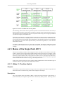
self-contained calibrations timed by instrumental performance and stability metrics. The currently designed Observing Modes and their relation to the AOTs is given in the following chart (Figure 4.1):
27
Observing with HIFI
Figure 4.1. Overview of available AOT observing modes.
The numbering scheme of the observing modes represents an association between the AOT class (in
Roman numerals) and four possible modes of reference treatment (Arabic numerals) that are foreseen.
The dual beam switch modes further split into two separate modes using a slow chopper speed (Mode
I-2) and a fast chopper speed (Mode I-2a).
Each Observing Mode uses a somewhat different scheme for the data processing including the intensity and frequency calibration depending on how the reference measurements are obtained while observing. Thus the noise level and the drift contribution to the total data uncertainty of the calibrated
data obtained from one of the AOTs depend critically on the Observing Mode (i.e., on the reference
measurement scheme).
To enable an educated selection of the AOT Observing Modes, the following subsections provide
descriptions of the scientific motives, typical usage, user options, data output, advantages and disadvantages.
4.2.1. Modes of the Single Point AOT I
There are four modes provided for observing point sources with HIFI. The best mode to choose depends on the kind of science being done and the situation of the target object. For example, a point
source well away from any diffuse cloud emission is likely to be best suited by a Dual Beam Switch
observation, where reference OFF source positions are taken close to the target object. However,
sources embedded within molecular clouds the use of a sky source for reference may not be possible
and an internal reference is better to use, e.g., a load chop observation.
In this section we describe the point source modes available for HIFI observations and indicate typical
situations in which a given point source mode may be chosen.
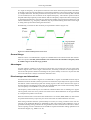
4.2.1.1. Mode I-1: Position Switch
Purpose:
Used to observe a point source (fixed or moving) in one or more spectral lines within a single IF band.
Allows the choice of a reference sky position within 2 degrees of the target.
Description:
This is the simplest Observing Mode for HIFI, in which the single pixel beam of the telescope is
pointed alternately at a target (ON) position then a reference sky (OFF) position. Observing is done
28
Observing with HIFI
at a single LO frequency, at the spectral resolution of the chosen back-end spectrometer. Data taken
at the OFF position provide the underlying system background that is removed in pipeline processing
by a simple subtraction. The OFF position is chosen by the user to be an area of the sky that is known
(or else assumed) to be free of emission at the requested frequency. The reference position must be
sampled sufficiently frequently so that detector drifts are adequately compensated. The switching rate
is calculated automatically in the AOT logic based on knowledge of the instrument stability time, and
internal calibrations (e.g., frequency calibration) may be performed during initial slews to the target
or during telescope movement during the observation.
Schematically, a timeline for this mode may be represented as follows (Figure 4.2):
Figure 4.2. Timeline of HIFI position switch AOT.
General Usage:
Ideal for sources in crowded fields or regions of extended emission for which accurate flux measurements are required. An OFF position which is free of emission at the selected LO frequency must
be within 2 degrees of the ON target position.
Advantages:
Accurate intensity calibration of the observed spectral line can be achieved if an area of the beam
within 2 degrees of the science target is emission-free, and timing constraints on the integrations at
the ON an OFF positions based on knowledge of the system stability are met in a way that the drift
term in the total noise is always less than the radiometric term.
Disadvantages and alternatives:
An emission-free area within 2 degrees of crowded fields or regions of extended emission may be
difficult to locate for the OFF (reference) position to be used. This is especially true for regions towards
the Galactic Centre and around popular star forming regions. If the closest emission-free region is
beyond 2 degrees, and mapping modes (AOT II) are undesirable, then a mode with load-chop (Mode
I-4) or frequency-switch (Mode I-3) may be more desirable.
The frequency switch mode may be more efficient if baseline effects such as standing wave ripples
can be ignored, in the case of very narrow lines where even a distorted baseline can be approximated
by a simple linear profile across the line.
If the astronomical source to be observed is smaller than 3 arc minutes, DBS (Mode I-2) observations
are preferred because they require only rare slews and contain an inherent baseline correction.
If the timing constraints from the system stability are not met, it is easily possible to arrive at an uncertainty of the calibrated data that is dominated by drift noise instead of the radiometric noise. In
general the resulting timing constraints do not guarantee accurate continuum level derivation. Observations requiring accurate continuum levels should be acquired with modes making optimum use of
the internal chopper (e.g., Mode I-2 or 2a).
29
Observing with HIFI
User Inputs:
Target (ON) and reference (OFF) positions, LO band and frequency, minimum and maximum goal
frequency resolution of the calibrated data, spectrometer usage, and total observing time or noise goal
at the lowest goal at the goal resolution.
Data Calibration:
The final spectra are based on the differences between neighbouring ON target and OFF reference
position measurements. Co-addition of (ON - OFF) provide the final 1D spectrum.
A zeroth order baseline may occassionally need to be subtracted when using this mode.
No explicit standing wave correction is needed.
Instrument tuning, frequency calibration, and measurements of the internal hot and cold loads will be
done during initial slew, and may be done during slews between ON and OFF positions depending
on slew length and rate.
The transformation into a brightness temperature scale is performed by dividing the difference measurement by the results from the load calibration measurements and multiplying by the corresponding
difference in the Rayleigh-Jeans temperatures of the hot and cold loads for the given LO band (loads
are measured during each observation).
The final translation into a beam temperature relies on the beam efficiency, as measured at the primary
calibration sources.
4.2.1.2. Mode I-2: Dual Beam Switch (DBS)
Purpose:
Used to observe a point source (fixed or moving) in one or more spectral lines or continuum within
a single IF band. Uses chopper to view fixed sky positions for reference, 3' either side of the target
position.
Description:
In this mode an internal mirror is used to provide the motion to a reference OFF position on the sky. The
reference OFF position is currently set to be 3 arc minutes from the ON target position, and is
not adjustable by the user. Moving the internal mirror changes the light path for the incoming waves,
subjecting the measurements to the possibility of residual standing waves, so moving the telescope
in such a way that the source appears in both chop positions is expected to completely eliminate the
impact of standing wave differences in the two light paths.
The low dead time in moving a small distance with the telescope and in the internal chopper motion
makes this mode more efficient than position switching (Mode I- 1). A diagram showing the telescope
and chopper positions is shown in Figure 4.3:
30
Observing with HIFI
Figure 4.3. HIFI Dual Beam Switch positions on the sky.
Two chopper speeds are available to the user, a slow chop mode with typically 0.125Hz chopper speed
(Mode I-2) and a fast chop DBS (Mode I-2a) with a frequencyup to 4Hz. The faster chop is intended
to compensate for instrumental drifts at low frequency resolutions that would otherwise (at the slow
chop rate) lead to baseline distortion and increased intensity uncertainties.
If accurate continuum level measurements are needed, e.g., for some absorption-line studies, then a
separate calibration scheme is selectable by the user to provide a stable continuum. Note that selection
of continuum stability timing in this mode can significantly reduce the efficiency of the observation, particularly at the highest frequencies in bands 6 and 7. A schematic timeline for Mode
I-2 appears in Figure 4.4:
Figure 4.4. Timeline of the HIFI Dual Beam Switch observing mode.
General Usage:
Point sources or slight extended (< 3' in diameter) objects that are not sitting within or near to extended
emission at the requested frequency.
Particularly useful for moderately distant to very distant extragalactic objects.
The fast chop mode (Mode I-2a) is expected to be used where accurate continuum or broad line (low
spectral resolution) measurements are required.
The initial results from comparing performances of the normal (or slow) chop DBS with FastDBS
modes indicate that the latter generally perform better with respect to correction for electrical standing
waves in bands 6 and 7. The recommendation at this time is to only use the FastDBS mode in the
HEB bands (bands 6 and 7).
31
Observing with HIFI
Advantages:
Accurate baseline removal with no trade-off with line intensity calibration accuracy by optical effects
(standing wave differences will cancel via dual chop motion). The internal chop measurements and
small telescope motions mean that the science target is viewed nearly 50 per cent of the time. This
is typically more efficient than the position switch method (Mode I-1). Fast chopping (Mode I-2a) is
best at lower spectral resolutions.
Disadvantages and alternatives:
Relative timing between the internal chopper and telescope nodding at all of HIFI's integration times
is crucial to avoid residual ripples, and the constraints cannot be tested and adjusted until the commissioning phase. Also, the direction of the chopper motion on the sky depends on the roll angle of the
spacecraft, which slowly changes on orbit. Thus the chopper motion is only predictable when fixing
the data and time of an observation, which is not advised in order to allow normal scheduling flexibility, meaning that the mode should be generally restricted to objects with a size below 3 arc minutes in
all directions. Otherwise the observations should use position switch, frequency switch or load chop
modes (Modes I-1, I-3, or I-4).
User Inputs:
Target (ON) position, chop rate (fast or normal), LO band and frequency, minimum and maximum
goal frequency resolution of the calibrated data, spectrometer usage, and total observing time or noise
limit at the lowest goal resolution.
It is possible to adjust the chopper speed via user inputs. When setting time estimates, the chopper
and dual-beam cycling speed is affected by the associated Allan time. For higher cycling use larger
goal resolutions, for which the Allan times are larger. This forces faster repetitions of the cycle. HSpot
messages available following time estimation indicate the achieved speed.
Data Calibration:
For the standard data reduction of dual beam switch observations the double difference has to be
computed between the counts in the two chop phases at one telescope position and the corresponding
difference for the second position. As two of the phases contain signal from the source, the total
radiometric signal to noise ratio of the calibrated data corresponds exactly to the value from one phase.
The mode thus has a maximum efficiency of 0.25 in the case of no dead times.
The double difference completely cancels out all standing wave contributions from the receiver noise
and from warm telescope components promising a perfect calibration of the underlying continuum or
a perfect zero-level baseline in case of sources with no continuum contribution. It also guarantees a
cancellation of all intensity drift effects that are purely linear within the corresponding cycle time.
An estimate of the total drift noise contribution can be obtained from the stability parameters of the
instrument measured in terms of an Allan variance spectrum. When all ON-OFF cycles are performed
with a sufficiently small period, it is guaranteed that the drift noise is small compared to the radiometric
noise of calibrated data.
The conversion into brightness temperatures is performed on the basis of the counts from the thermal
load measurements.
4.2.1.3. Mode I-3: Frequency Switch with optional OFF calibration
Purpose:
Used to observe a point source (fixed or moving) in one or more spectral lines within a single IF
band. Uses a switching between two LO frequencies for reference. Useful when no sky references
immediately near by. Can not be used for continuum measurements. It is highly recommended that
users always use an OFF reference position whenever possible with this mode.
32
Observing with HIFI
Description:
In this mode, following an observation at the requested frequency, the LO is adjusted by a generally
small amount (a frequency 'throw' as specified by the user) causing the spectral region sampled by
the spectrometers to likewise be adjusted by the same frequency throw. The frequency shift should be
chosen so that it is small enough that the lines of interest remain observable at the two LO frequencies
and that lines do not overlap from the two phases. Differencing of the two spectra can be used to
effectively remove the baseline. Since the second frequency position also contains lines of interest,
these appear as inverted lines in the difference measurement.
The mode is very efficient, since target emission lines are observed in both frequency positions. However, the system response is likely to differ between the two frequency settings and simple spectrum
arithmetic may not result in clean baseline removal, and may potentially leave significant ripples in
the difference spectrum. This should be mitigated by observing both frequencies also at an OFF sky
position at the same two frequencies.
The mode allows the user to specify a suitable OFF position, which should be free of emission/absorption line features. It is highly encouraged that an OFF position be employed by users of this mode
and good reason should be supplied in the proposal justification if no OFF position is to be used.
This is especially true for the diplexer Bands 3 and 4, in which the standing waves are not wellfitted by one or two sine waves of constant amplitude. Only if the User expects very strong lines
and is not concerned by the standing wave pattern in the surrounding baseline, or expects to be
able to fit the standing waves in IA when the lines are narrow, should the "no reference" option
be considered. This mode is more appealing for observations of complex astronomical environments,
where baseline removal cannot be accomplished with an immediately spatially available emission-free
reference OFF measurement, as compared to the position switching or DBS modes (Modes I-1 and
I-2). A schematic timeline of frequency switch measurements is shown in Figure 4.5:
Figure 4.5. Timeline for HIFI Frequency Switch observations.
General Usage:
Sources with relatively simple spectra, either extended or located in complex environments such that
region free of emission at the selected LO frequency cannot be defined with either 2 degrees (for
position switching) or 3 arc minutes (for DBS). Observations of giant HII regions and molecular clouds
in Galactic star-forming regions may rely extensively on this mode.
This mode is not recommended in HEB Bands 6 and 7, due to poor stability in terms of baseline
shapes, ripples, and artefacts that may not be treatable in IA such that S/N goals set by the User
in HSpot can ever be achieved, and may thus compromise the intended science goals. At this
time, the recommendation is to use the alternative Load Chop mode in the HEB bands.
Advantages:
A potentially very efficient mode, with the science target lines almost always being integrated on
during the observation and low dead time expected for retuning the LO repeatedly between requested
and offset frequencies. Expected to be good for baseline characterisation and removal in regions of
extended sub-mm emission.
33
Observing with HIFI
Disadvantages and alternatives:
System response differs between requested and offset frequencies. The differences in flight verify
that the scheme for observing a sky OFF position at the same frequencies to compensate for residual
standing waves in the ON target difference measurements is a very strong recommendation.
It should not be used for sources with rich spectra or very broad lines, which would make it impossible
to deconvolve the contribution of both phases from the difference spectrum, preventing any reliable
data reduction.
If these conditions cannot be met, and no emission-free region is nearby, or timing constraints in the
logic for this Observing Mode are too difficult, then the load chop mode with OFF calibration (Mode
I-4) is expected to be a better option.
User inputs:
Target (ON) position, optional reference (OFF) position, LO band and frequency, frequency throw
(see Table 4.1), minimum and maximum goal frequency resolution of the calibrated data, spectrometer
usage, and total observing time or noise limit at the lowest goal resolution.
Table 4.1. Frequency throw values available by HIFI subband. Frequency throws have been optimised
during early in-flight testing in each subband.
Band
Large negative (MHz)
Small negative (MHz)
Small positive (MHz)
Large positive (MHz)
1a
-288
-94
+94
+288
1b
-288
-94
+94
+288
2a
-288
-94
+94
+288
2b
-288
-94
+94
+288
3a
-288
-94
+94
+288
3b
-288
-94
+94
+288
4a
-288
-94
+94
+288
4b
-288
-94
+94
+288
5a
-300
-98
+98
+300
5b
-300
-98
+98
+300
6a
-192
-96
+96
+192
6b
-192
-96
+96
+192
7a
-192
-96
+96
+192
7b
-192
-96
+96
+192
Data Calibration:
Frequency-switched observations will be calibrated in two main steps:
• standard calibration resulting in a difference spectrum, and
• the coaddition of the contributions from both phases.
For the second step, several common software tools will be available to the user, but the result has to
be interpreted with care by the user based on available knowledge of the expected source spectrum.
It is in general not possible to generate a 'normal' spectrum representing only one frequency phase
from the difference spectrum. In the simplest approach, shift-and-subtract, the difference spectrum is
shifted relative to itself by the frequency switch step and subtracted, resulting in calibrated lines with
the best possible signal to noise ratio, but where each line is accompanied by 'ghost' lines with the
34
Observing with HIFI
opposite sign which cannot be easily removed. None of the more sophisticated methods are expected
to completely eliminate this problem. This can also be achieved via the "doFold" task in HIPE.
For the basic calibration of the difference spectrum (step 1), the difference of the measurement between
the two phases on the OFF position is subtracted from the ON source difference, but in contrast to the
load-chop mode, this double-difference is not taken from the pure spectrometer counts. Rather each
measurement is translated individually into a temperature scale by applying the load-calibration for
the corresponding frequency setting. Their mutual difference is computed only in the second step.
The double difference potentially cancels out all standing wave differences between the two phases,
but a perfect zero-level baseline is only obtained if the system response, as measured with the load
calibration measurements, agrees relatively well between the two frequency switch phases, which is
not guaranteed (or at least not quantified until flight).
The double difference also guarantees a cancellation of all intensity drift effects that are purely linear within the corresponding cycle time. However, additional spectral noise will result from the double-difference, and extra analysis time is likely to be required for the baseline calibration measurement, which will add to the noise in the calibrated data. This may represent a considerable overhead
if the goal frequency resolution of the observation is not much smaller than the resolution needed to
determine possible standing wave ripples in the system.
4.2.1.4. Mode I-4: Load Chop with optional OFF calibration
Purpose:
Used to observe a point source (fixed or moving) in one or more spectral lines within a single IF
band. Uses the internal loads for reference. It is highly recommended that users always use an OFF
reference position whenever possible with this mode.
Description:
In this reference scheme, an internal cold calibration source is used as a reference to correct short term
changes in instrument behaviour. The HIFI chopping mirror alternately looks at the target on the sky
and an internal source of radiation with a typical period of a few seconds. This is particularly useful
when there are no emission-free regions near the target that can be used as reference in either
position switch or dual beam switch modes (Modes I-1 and I-2) or where frequency switching
(Mode I-3) cannot be used due to the spectral complexity of the source.
Since the optical path differs between source and internal reference, a residual standing wave structure
may remain. Additional measurements of an OFF measurement of an emission-free region (chosen
by the user) can be used to reduce baseline ripple. Such a scheme is robust but has relatively high
dead times.
The total time spent on the OFF position depends on the frequency resolution needed to describe the
baseline ripple which may be considerably smaller than the integration time spent on the source.
The general timeline is illustrated by the following schematic picture (Figure 4.6):
Figure 4.6. Timeline for the HIFI load chop observing mode.
35
Observing with HIFI
General Usage:
Sources with a high density of emission/absorption lines that lie within extended emitting regions. Like
the Frequency Switch mode, Load Chop is recommended to be used only with the sky reference
option to obtain a spectrum at a User-selected line-free region (within 2 degrees of the science target)
for standing wave correction in the pipeline. This applies most strongly to Bands 3, 4, 6, and 7, and/
or in cases where lines may be too broad for interactive ripple fitting.
Advantages:
This is an efficient mode for measurements of sources in extended emission regions. With OFF reference, the mode can be used as a fall-back for observations that would normally use a position switch
but where the distance to the OFF position would require a slew time comparable to the total on source
integration time. With use of an OFF position, in principle, all pointed observations could be done
with this robust mode, at the expense of higher dead times.
Disadvantages and alternatives:
Generally inefficient with typically 1/3 to 1/4 of the total time spent on the actual science target (time
on the OFF position is less than that on the target). However, this is a mode which attempts to provide
robust calibration of data for the most spatially and spectrally complex targets in single pointing modes,
and therefore no further alternatives are offered.
User inputs:
Target (ON) position, optional reference (OFF) position, LO band and frequency, minimum and maximum goal frequency resolution of the calibrated data, spectrometer usage, and total observing time
or noise limit at the lowest goal resolution.
Data calibration:
The observing mode of load-chop observations with an OFF calibration is extremely robust with respect to calibration uncertainties, because it uses a double difference to determine the flux from the
astronomical source relative to the flux from the sky on the OFF position. The double difference completely cancels out all uncertainties in standing wave contributions from the receiver noise and from
warm telescope components, promising a perfect calibration of the underlying continuum or a perfect
zero-level baseline in case of sources with no continuum contribution.
The mode also guarantees a cancellation of all intensity drift effects that are purely linear within the
corresponding cycle time.
This robustness is, however, obtained at the cost of an increased spectral noise produced by the double-difference. If the period of standing waves in the system is equal to or less than the desired frequency resolution of the observations, the observing time has to be doubled to obtain the same signal-to-noise ratio as compared to observations without baseline calibration. Many observations will,
however, require a frequency resolution that is finer than the standing wave ripple so that the overhead
from the baseline calibration is smaller.
If the user chooses to opt out of the OFF reference measurement, then a residual baseline (including
ripple) is likely to remain and may require removal interactively by the user.
4.2.2. Modes of the Mapping AOT II
There are four mapping modes available to HIFI. The "On-the-Fly" observing mode takes data continuously as a source is scanned and can use a frequency switch reference, a load chop reference or a
sky reference, while a dual beam switch (DBS) raster map takes data at set points on a user-defined
grid. A variant of the DBS raster map, a small 5-point raster cross map was originally made available
but has now been discontinued.
36
Observing with HIFI
4.2.2.1. Mode II-1: On-the-fly (OTF) Maps with Position-Switch Reference
Purpose:
Used to observe an extended source (fixed or moving) in one or more spectral lines within a single IF
band. Allows the choice of a reference sky position within 2 degrees of the target.
Description:
The observing mode of OTF-maps with position-switch reference is in many cases the most efficient
observing mode for mapping observations with HIFI. Because one reference measurement can be used
for several source measurements and little time is lost to telescope motions without data integrations,
it can in principle approach an observing time efficiency of 100 per cent.
The system instability is taken into account here by the repeated observation of an OFF position which
is either free of emission or has a well known emission profile. The mode is relatively insensitive to
standing wave problems because only one optical path is used.
While the telescope scans any particular row of the map, permanent data readouts are made at regular
time intervals. The time intervals are set such that the telescope scan covers the width of a single point
in the output map (default is Nyquist sampling distance). The source integration is performed during
the whole scan except for very small breaks for the data readout.
After each row, the telescope motion changes its orientation so that the next row will be scanned in the
opposite direction. The integration of instrument data is stopped during these turns (taking serendipity
data might be possible, but this should not interfere with the optimum start and stop times for the
integration within each row).
After a period determined by the system stability time, the scanning of the map is interrupted for the
reference measurement on the OFF position. Reference measurements are only taken after an integral
number of scan legs.
Changes in the instrumental sensitivity are measured in the frame of a fourth loop using the known
difference in the radiation field between hot and the cold internal loads. This load calibration is performed during slews to the OFF position.
The efficiency of the mode profits from high scan velocities, the map will be typically observed in a
series of multiple coverages adding up to the required total integration time per source position.
The time line of the observation consists of motions of the telescope across the map and between
the map and the OFF position, integrations of the instrumental output during the different phases and
interleaving load calibration measurements. Figure 4.7 shows the timeline for the OTF mapping mode.
Figure 4.7. Timeline of the path on the sky for a HIFI OTF mapping mode. The green dots indicate regular
data readouts of the spectrometers. The OFF position is returned to at the end of an integer number of
scan legs. This is typically 1 or 2 except in the case of small OTF maps.
37
Observing with HIFI
In the example shown in Figure 4.7, the OFF position is visited three times within one coverage of
the whole map, after every two scanned lines. It is planned to always complete full scan lines before
an OFF observation. A series of subsequent coverages will be performed with one extra OFF measurement at the end of the observation guaranteeing a complete enclosing of the source observations
by OFF observations. The green dots symbolise the points where the spectrometers are read out. The
integration starts as soon as the telescope enters the blue area of the map. Note the change of the
scanning direction after each row.
For situations where an emission-free OFF position is not immediately available, the OTF scan with
load chop (scanning and comparing to frequent load measurements) or frequency switch (similarly,
scanning and switching frequency) may preferably be used. This is particularly useful for mapping
using bands 6 and 7, where the short stability times mean that significant drifts can occur during a
map scan leg. Continuous reference to the internal load during a scan leg (for example) can help
mitigate against such drifts and the increased associated with the drifts
Advantages:
On-the-Fly scanning should be considered the standard mode for astronomical mapping with HIFI. It
provides the most efficient mapping scheme for HIFI. Load chop and frequency switch versions can
be useful in complex regions and when stability times are short (e.g., in the HEB bands, 6 and 7).
Disadvantages and Alternatives:
Its use is problematic if no nearby position can be defined for an OFF position which is free of emission.
In this case it is often still possible and efficient to use an auxiliary nearby OFF position, the emission
of which is determined by a separate position-switch observation.
However, if the closest emission-free region is too distant from the area to be mapped, OTF modes
with frequency switch can be more efficient. The same holds in all cases where the scientific aim
of the observation does not require an accurate treatment of baseline effects, ignoring standing wave
ripples or other baseline distortions. This will be the case for observations of very narrow lines where
even a distorted baseline can be approximated by a simple linear profile across the line. In such cases
OTF maps with frequency switch can be more efficient, but not good for broader lines, where the load
chop version of OTF is better.
It will not be possible to determine the continuum level from OTF maps. If continuum mapping (for
a small region) is required then the DBS raster map should be used.
User inputs:
The user has the possibilities of rectangular map sizes, scan length (X) and cross-scan map size (Y).
The cross-step can be set at Nyquist sampling or one of a number of set cross-step sizes (in arc seconds).
The user is also asked for the position of an OFF reference source, which is mandatory.
Data calibration:
The reference for each scan map point is based on a combination of prior and following OFF position
measurements. Because of instrumental limitations with respect to data rates, the speed of the telescope motion, and the gain instabilities, it will not be possible to obtain an accurate determination of
the continuum level from observations in OTF-maps with position switch reference. The subtraction
of a zeroth order baseline should always be expected although the baseline itself does not need to be
calibrated as the same optical path is used for source and reference. Observations aiming at a determination of the continuum level have to rely on modes using the internal chopper such as the raster scan.
4.2.2.2. Mode II-2: Raster Maps with Dual Beam Switch
Purpose:
Used to observe a small an extended source (fixed or moving) in one or more spectral lines or continuum within a single IF band. Uses the fixed 3' sky reference positions either side of each raster
position which limits the effectively useful size of a raster.
38
Observing with HIFI
Description:
In this mode, a grid of positions are each measured using a dual beam switch method. The mode works
for each grid position in the same way as for the point source dual beam switch mode (see Mode I-2).
The beam switch samples sky at 3 arc minutes either side of each grid position, with a telescope
movement occurring between changes to the beam switch either side of the grid position. With this
setup, large maps would find the beam chopping into the field of view, so this is not a good mode for
doing large extended emission region mapping.
Advantages:
It is a good mode for situations where fast (chopping) references are needed, as may be the case
for band 6 and 7 measurements, or where continuum measurements are required for small extended
sources or point sources. In these cases, scanning measurements may take too long allowing drifts
to occur.
Disadvantages and Alternatives:
Not as efficient as OTF mapping and, with a beam switch of only 3 arc minutes, this is not a good
mode to use for large-scale maps.
Limited to 32x32 raster points in a single observation.
User inputs:
The user has the possibilities of rectangular map sizes, scan length (X) and cross-scan map size (Y).
The cross-step can be set at Nyquist sampling or one of a number of set cross-step sizes (in arc seconds).
Continuum timing (for accurate baseline measurements) and fast chopping are selectable.
Data calibration:
Each raster map position can be calibrated in the same way as single point dual beamswitch data (see
Section 4.2.1.2).
4.2.2.3. Mode II-2X: Cross Map with Dual Beam Switch (currently
unavailable)
Purpose:
Used to observe spectral lines or continuum in a point source for which the most accurate flux is needed
but for which the position or pointing inaccuracy could cause significant error in the measurement.
Uses sky references 3' either side of the target. Note that this mode is currently unavailable pending
a fix to its commanding -- it has had few science observation requests in the Key Project calls.
Description:
In this mode, a cross grid of set positions forming a 5-point cross are each measured using the dual
beam switch method. The separation of the cross positions is selectable as "pointing jitter" (to represent
the possible worst-case pointing error of the observatory, currently set at 3"), "Nyquist" (for Nyquist
sampling of the beam size for the chosen frequency), and "10", "20" or "40" arcseconds. The mode
works for each grid position in the same way as for the point source dual beam switch mode (see
Mode I-2).
The beam switch samples sky at 3 arc minutes either side of each grid position, with a telescope
movement occurring between changes to the beam switch either side of the grid position.
Advantages:
Can improve the accuracy of flux measurements for point sources for any cases where the pointing
error or known position is large compared to the beam size.
39
Observing with HIFI
Provides basic flux and spatial information on small extended sources.
Disadvantages and Alternatives:
Can not be used for large maps and not a good means for obtaining accurate total flux information for
extended sources. For accurate pointing and for objects with well known positions, some time is lost
since the telescope beam is slightly offset from the target position for each of the cross positions.
User inputs:
Continuum timing (for accurate baseline measurements) and fast chopping are also selectable.
Data calibration:
Each cross map position can be calibrated in the same way as single point dual beamswitch data (see
Section 4.2.1.2).
4.2.2.4. Mode II-3: OTF Maps with Frequency Switch
Description:
In this mode, a scan map is made across a source, during which frequency switching is introduced..
The mode works for each scan map position in the same way as for the point source frequency switch
mode (see Mode I-3).
Advantages:
It is a good mode for situations where fast (chopping) references are needed, as may be the case for
band 6 and 7 measurements. An efficient mode for mapping of extended line emission regions since
telescope slews to an OFF position are not necessary and the target grid positions are always being
measured (at slightly offset frequencies). Particularly useful for mapping large regions of line emission
where a DBS measurement (see Mode II-2) would have "contaminating" emission in the reference
beams.
Disadvantages and Alternatives:
The scheme has similar disadvantages to the single point frequency switch mode (see Section 4.2.1.3).
System response will almost certainly be different at the requested and offset frequencies in a way
which cannot be calculated from laboratory measurements. This may lead to residual standing waves.
User inputs:
The user has the possibilities of rectangular map sizes, scan length (X) and cross-scan map size (Y).
The cross-step can be set at Nyquist sampling or one of a number of set cross-step sizes (in arc seconds).
The frequency throw is selectable by the user.
Data calibration:
Each OTF map position can be calibrated in the same way as single point frequency switch data (see
Section 4.2.1.3).
4.2.2.5. Mode II-4: OTF Maps with Load Chop
Description:
In this mode, a scan map is made across a source, during which chopping against internal loads also
takes place. The mode works for each scan map position in the same way as for the point source load
chop mode (see Mode I-4).
40
Observing with HIFI
Advantages:
It is a good mode for situations where fast (chopping) references are needed, as may be the case for
band 6 and 7 measurements and for when frequency switching is made difficult by the density of
spectral lines or the expected existence of broad lines. It is an efficient mode for mapping of extended
line emission regions since telescope slews to an OFF position are not necessary and the target grid
positions are always being measured (at slightly offset frequencies). Particularly useful for mapping
large regions of line emission where a DBS measurement (see Mode II-2) would have "contaminating"
emission in the reference beams.
Disadvantages and Alternatives:
The scheme has similar disadvantages to the single point load chop mode (see Section 4.2.1.3). The
changing light path between observing loads as opposed to the sky can lead to residual standing waves.
User inputs:
The user has the possibilities of rectangular map sizes, scan length (X) and cross-scan map size (Y).
The cross-step can be set at Nyquist sampling or one of a number of set cross-step sizes (in arc seconds).
Data calibration:
Each OTF map position can be calibrated in the same way as single point load chop data (see Section 4.2.1.4).
4.2.3. Modes of the Spectral Scan AOT III
Spectral scans consist of a series of observations of a fixed single target at several frequencies using
the WBS as main backend. After data processing, the result of such an observation will be a continuous
single-sideband (SSB) spectrum for the selected position covering the selected frequency range. The
LO tuning will be advanced in small steps across a single LO band. From a data analysis standpoint,
the reduction to a SSB spectrum is most reliable when the number of frequency settings within the
instantaneous bandwidth of the instrument is high, i.e. the frequency coverage is redundant. This must
be balanced with the loss of observing efficiency imposed by the dead times associated with retuning to
each new LO frequency. For most sources, a reliable reduction of the line spectrum requires at least 5
frequency settings within the IF bandwidth, i.e. a redundancy of 4. The spacings between the different
LO frequencies have to contain a small random component to prevent harmonics which could occur
in the reduction of the multiple double-sideband measurements to a single sideband (SSB) spectrum
in a deconvolution process.
This mode can use either a frequency switch (FS) or dual beam switch (DBS) reference frame to
compensate for instrumental drifts.
4.2.3.1. Mode III-2: Dual Beam Switch Spectral Scan
Purpose:
Used to observe a point source (fixed or moving) over a large frequency range (> 20GHz) by the use
of multiple LO frequency settings during the observation. Uses the dual beam switch sky referencing
scheme, sky positions 3' either side of the target.
Description:
The use of DBS reference inherits all the advantages and restrictions from the single point dual beam
switch observing mode (Mode I-2). The combination of telescope and chopper motions follows the
same scheme and timing constraints as Mode I-2. This implies also that this spectral scan mode can
only be applied to astronomical sources that are smaller than the chop angle of 3 arc minutes. Each LO
41
Observing with HIFI
frequency is separately calibrated against the internal hot/cold loads of the instrument. Extra observing
time is spent at LO frequencies where the system temperature is significantly degraded with respect
to the rest of the LO subband being used.
The user may choose to do all or part of a spectral range within a given band.
NOTE: it is advised that the fast DBS chopping mode be used in association with bands 6 or 7 spectral
scans.
Advantages:
Fast chop and continuum timing options allow for continuum measurements which are not possible
with the frequency switch version of the spectral scan. Thus also the most useful for measuring absorption line strengths.
Disadvantages and Alternatives:
The scheme has similar restrictions to other dual beam switch (DBS) measurements. For extended
sources the chopped beam is likely to land in an emission region. Fast chop is required when the stability (Allan) times at the goal resolution of the system are less than 2 seconds. This reduces observing
efficiency.
User inputs:
The user has choice of frequency range within the mixer band frequency range chosen (partial or full
band). The user can choose a redundancy of between 2 and 12. Higher values increase the fidelity of
the final single sideband spectrum expected from the data reduction of the mode but also make the
mode less efficient. Fast chop and continuum timing for the DBS mode used are also available options.
Data calibration:
Data reduction consists of two parts: the calibration of the double sideband spectrum (see Section 4.2.1.2) and the deconvolution of the set of double sideband spectra into a single sideband spectrum. The calibration of the double sideband spectrum is identical to the calibration in the single point
with dual beam switch (see Section 4.2.1.2) applied for spectra taken at each LO setting
Sideband deconvolution is provided via a data software task provided within the HIPE software environment and takes place after each double sideband spectrum has been processed. More information
on the sideband deconvolution software are noted in Chapter 6.
No "ghost lines", symptoms of instabilities or insufficient sampling, have been found in any spectral
survey so far. When spectral artefacts and bad baselines are removed completely from the input prior
to using the deconvolution algorithm in post-processing, the deconvolution yields flat baselines with
neither ringing, nor any added repetitive noise structures.
4.2.3.2. Mode III-3: Frequency Switch Spectral Scan
Purpose:
Used to observe a point source (fixed or moving) over a large frequency range (typically > 20GHz) by
the use of multiple LO frequency settings during the observation. But can also be used to get smaller
ranges where the different LO settings allow the distinguishing of spectral features into upper and
lower sidebands. Uses frequency switching for reference.
Description:
This mode behaves in a similar fashion to the DBS version of mode III-2. The reference used is from
a nearby frequency, using a small step frequency away from each of the main steps that are taken
42
Observing with HIFI
every 0.5 to 1GHz. The mode inherits similar advantages and disadvantages to mode I-3. The pattern
of spatial and main frequency groupings is similar to mode III-2 (also see ???).
Advantages:
Most useful for line observations of objects that are in regions of extended emission. Since the object
is always being measured, it is a more efficient mode than mode III-2.
Disadvantages and Alternatives:
The scheme has similar disadvantages to the single point frequency switch mode (see Section 4.2.1.3).
System response will almost certainly be different at the requested and offset frequencies in a way
which cannot be calculated from laboratory measurements. This may lead to residual standing waves.
Continuum measurements can not be made with this mode without an OFF position measurement to
calibrate the baseline. Mode III-2 is preferable for measurements where the baseline continuum is
needed to be accurately measured.
User inputs:
The user has choice of frequency range within the mixer band frequency range chosen (partial or full
band). The user can choose a redundancy of between 2 and 12. Higher values increase the fidelity of
the final single sideband spectrum expected from the data reduction of the mode but also make the
mode less efficient. The frequency throw is also an input choice for the user.
Data calibration:
Data reduction consists of two parts: the calibration of the double sideband spectrum (see Section 4.2.1.3) and the deconvolution of the set of double sideband spectra into a single sideband spectrum. The calibration of the frequency switch spectra is identical to the calibration in the single point
with frequency switch (see Section 4.2.1.3). The load measurements for the bandpass calibration are
taken at exactly the same LO frequencies as the data.
Sideband deconvolution is provided via a data software task within the HIPE software environment
and must be run interactively by the user after each double sideband spectrum has been processed.
More information on the sideband deconvolution software is noted in Chapter 6.
4.2.3.3. Mode III-4: Spectral Scan with Load Chop
Purpose:
Used to observe a point source (fixed or moving) over a large frequency range (typically > 20GHz) by
the use of multiple LO frequency settings during the observation. But can also be used to get smaller
ranges where the different LO settings allow the distinguishing of spectral features into upper and
lower sidebands. Uses the internal HIFI loads for reference during the measurements.
Description:
This mode behaves in a similar fashion to the load chop single point mode I-4. The reference used is
from the internal cold load and measurements are for every LO frequency of the scan (typically every
0.5 to 1 GHz or so).e effects An OFF position should be used that can be up to 2 degrees away from
the target, where similar measurements can be made to allow a double-differencing that removes the
effects of light path differences of sky to mixer and sky to internal load. The mode inherits similar
advantages and disadvantages to mode I-4. The pattern of spatial and main frequency groupings is
similar to mode III-2 (also see ???).
Advantages:
Most useful for line observations of objects that are in regions of extended emission and where a
fast referencing scheme is preferred (e.g., using bands 6 and 7). Particularly useful for sources where
43
Observing with HIFI
there is expected to be high line complexity. The use of the OFF position is highly recommended for
removing standing waves.
Disadvantages and Alternatives:
The scheme has similar disadvantages to the single point load chop mode (see Section 4.2.1.4). The
light path difference of load-to-mixer and sky-to-mixer means that residual standing wave differences
typically remai. This can be mitigated with the use of a reference OFF position measurement which
is of an area free of emission. Continuum measurements can not be made with this mode without an
OFF position measurement to calibrate the baseline. Mode III-2 is preferable for measurements where
the baseline continuum is needed to be accurately measured.
User inputs:
The user has choice of frequency range within the mixer band frequency range chosen (partial or full
band). The user can choose a redundancy of between 2 and 12. Higher values increase the fidelity of the
final single sideband spectrum expected from the data reduction of the mode but also make the mode
less efficient. The position of the reference OFF is a choice of the user (within 2 degrees of the target).
Data calibration:
Data reduction follows that of the point load chop mode (see Section 4.2.1.4) for each LO frequency
used in the scan. This is followed by the deconvolution of the set of the calibrated double sideband
spectra into a single sideband spectrum.
Sideband deconvolution is provided via a data software task within the HIPE software environment
and must be run interactively by the user after each double sideband spectrum has been processed.
More information on the sideband deconvolution software is noted in Chapter 6.
4.3. Standing Wave Residuals after Calibration (Pipeline Level 2)
The HIFI pipelines are designed to correct for standing waves in the astronomical data using off-source
sky spectra taken in AORs using any of the observing modes that include OFF-source sky measurements, i.e., telescope nodding plus chopping with the internal M3 mirror using fixed throws on the sky
(the DBS modes), or else telescope nodding to a User-selected reference sky position (modes using
a position switch). Here we present a summary of residual standing waves in that remain following
standard pipeline processing (up to Level 2 products provided in the Herschel Science Archive, HSA).
The information is based on data taken with the Point AOTs that have all been reference-corrected in
the standard fashion. Frequency Switch and Load Chop observations have all included the sky reference option in HSpot (recommended). [Approximations can be made in IA for skipping this option
to a corresponding "No Ref" version as allowed in HSpot, by simply skipping the sky correction step
in the pipeline.]
Attempts to remove these waves in HIPE are also discussed. Because the wave characteristics differ
between bands with beam splitters and diplexers as well as between SIS and HEB mixers, they are
discussed separately. The conclusions are based on the limited dataset available from the HIFI performance verification phase.
4.3.1. Bands 1-5 (SIS mixers)
Bands 1-5 data taken in DBS mode generally do not show standing waves at Level 2. Exceptions are
sometimes observed, however, and in these cases the User can remove the waves with the sine wave
fitting task 'FitHifiFringe' in HIPE.
Two cases are shown below.
44
Observing with HIFI
• In Band 4b the diplexer causes a 650 MHz ripple. Figure 4.8 shows a sine wave fit (red) relative to
a baseline (green), automatically determined with the 'FitHifiFringe' routine.
• Strong continuum sources show the effect of ripples in the passband calibration. The periods are
typically in the 90-100 MHz range, and the amplitudes are at most 2% relative to the continuum.
See Figure 4.9 below for a case where 92 and 98 MHz since waves are present.
Figure 4.8. Standing wave residual at Level 2 in a DBS observation, with the fitted sine wave (red) relative
to a smoothed baseline (green)
Figure 4.9. Strong continuum source with two standing wave components at 92 and 98 MHz (red), relative
to the baseline (green).
45
Observing with HIFI
4.3.2. Position Switch, Frequency Switch and Load
Chop modes
Calibrated observations taken with the simple Position Switch, Frequency Switch (with OFF reference), or Load Chop (with OFF reference) modes in beamsplitter Bands 1, 2, and 5 also show clean
spectra. If any residual waves are present in the Level 2 products, they have the shape of pure sine
waves and can be subtracted using the 'FitHifiFringe' task in HIPE.
Observations in diplexer Bands 3 and 4 often show residual waves with larger amplitudes compared to
the DBS modes. Waves generated in the diplexer rooftop are not pure sine waves. Amplitudes increase
strongly toward the IF band edges. It is thus always advised to place the line of interest near the middle
of the IF band when possible, in WBS sub-bands 2 or 3. Although 'FitHifiFringe' only fits sine waves,
fits to the diplexer waves can be approximated using multiple sine waves, typically around 600 MHz.
The approximation is not as good at the IF band edges. Figure 4.10 and Figure 4.11 show examples
for Band 3b and 4b. Note that the baseline is strongly curved in both observations, and the user will
need to remove these separately in HIPE, using polynomial fitting.
Figure 4.10. Band 3b observation using Point Frequency Switch at Level 2 after sky subtraction (left) and
after interactive fringe fitting and removal (right). Note the poor edges in the IF spectrum on the right.
Figure 4.11. Band 4b observation using Point Frequency Switch, showing a strong residual standing wave
(black). Its period (~600 MHz) and increasing amplitude toward the band edges are those expected for
diplexer bands. It was fitted with a combination of sine waves using FitHifiFringe (green). The corrected
spectrum (red) still shows a strongly curved baseline that can be subtracted with a polynomial fit in HIPE.
46
Observing with HIFI
4.4. Bands 6-7 (HEB mixers)
The HEB mixers generate waves with characteristics that depend on the mixer current level, but since
there is a dependence on LO power which may not be stabilized (between ON and OFF spectra), both
electronic and optical standing wave residuals can be mixed together. Data taken with all observing
modes analyzed so far show residuals at Level 2, where the non-DBS modes tend to show larger and
more complex residuals.
4.4.1. DBS Modes
Bands 6-7 are less stable than bands 1-5, and Level 2 data occasionally show residual waves. Examples
are shown in Figure 4.12 for portions of Bands 6a and 7b. The latter was box-car smoothed by 5
channels.
Figure 4.12. Standing wave residuals in Bands 6a (left) and 7b (right).
These 'electronic' standing waves have periods of ~300 MHz, but they are not sine waves and 'FitHifiFringe' can only approximately remove them. A promising method ('current matching technique') is
being developed to remove these waves in the pipeline.
As for the presence of these waves the following general guidelines can be given:
• Band 6b is most stable and is least affected.
• FastDBS mode spectra tend to show weaker standing waves than 'slow chop' DBS mode spectra.
• In Band 7, spectra taken with the vertical polarization spectrometers tend to show stronger waves
than from the horizontal polarization. Sometimes this effect is very strong. See e.g., Figure 4.13.
Figure 4.13. Standing wave pattern in the Level 2 in Band 7a for WBS-V (red) and WBS-H (blue).
47
Observing with HIFI
4.4.2. Position Switch, Frequency Switch and Load
Chop Modes
Non-DBS observations show rather strong residuals in Level 2 spectra. An effort is under way to provide alternative processing of HEB band observations such that appropriate OFF spectra are selected
from a database of observations based on mixer current level (the 'current-matching' technique). This
approach should reduce the amplitudes of the residual standing waves considerably, but is currently
in development. Presently, the user may apply FitHifiFringe to remove the waves in Level 2 spectra.
This method has limitations, because the HEB waves are not pure sine waves: they disperse over the
IF band (i.e. their 'phase' changes). Figure 4.14 provides an example for HEB measurements using
the Point Load Chop mode. As can be seen, the line shape in the WBS-V and WBS-H spectra differ
somewhat after subtracting the sine-wave fit. This highlights another limitation of 'FitHifiFringe': for
broad lines covering much of the IF, insufficient surrounding baseline may be left to obtain accurate
sine wave fits. In addition, as for the diplexer bands, solutions are less accurate for lines close to the
IF band edge.
Figure 4.14. A Band 6a Point Load Chop observation showing residual waves after standard level 2 pipeline
processing (left), and after standing wave removal using FitHifiFringe (right). The fringe-corrected spectrum has been shifted and a small scaling applied along the intensity axis so that the H and V peaks agree.
4.5. "Grouping" or "Clustering" of Observations
At the present time, spatial clustering of targets into a single observation is NOT available for HIFI
observations.
A limited grouping of observations in a single band with a given setup but a limited number of frequencies is currently planned to be available at a later date.
4.6. Solar System Target Modes
All modes available for fixed targets (noted above) are available for moving targets also. One restriction on solar system targets is that fixed positions used as references can NOT be used. All OFF reference positions must be expressed as being relative to the target.
48
Chapter 5. HIFI Calibration
5.1. Introduction:
This chapter gives a general view of the calibration concepts chosen for the HIFI instrument. This
chapter is intended to provide an overview of how HIFI is calibrated the full details of which are
contained elsewhere but are referenced in this chapter.
Further calibration information of use to users will also continue to be placed in a calibration page
available via the Herschel Science Center wesbite at http://herschel.esac.esa.int.
The HIFI calibration approach can be broken down into three main areas:
• intensity calibration
• frequency calibration
• spatial response calibration
It is the combination of each of these three steps that provides the most accurately calibrated HIFI
spectrum (see summary in section Section 5.5). For each of these areas, a framework document has
been produced, describing in extensive details the calibration strategy and equations applying to HIFI.
In the following, we summarise the content of this framework.
5.2. The Intensity Calibration of HIFI
The framework for the intensity calibration description of Herschel/HIFI is given in [10]. This document defines the parameters at play in the intensity calibration approach and the various assumptions
allowing the simplification of the formalism. Here we provide an outline of the main components of
the HIFI calibration framework.
5.2.1. Context
In essence, the HIFI intensity calibration approach inherits from the chopper wheel method introduced
by Penzias and Burrus ([14]), which consists of relating backend counts of a differential (on-off)
source observation to the output of a hot (also called the chopper) stable temperature load compared
to that of a colder one (originally, the blank sky). Compared to this standard scheme, HIFI faces
the simplification that all contributions and instabilities from the atmosphere can be neglected. Also,
many of the approximations used by the standard approach are not valid for systems with large IF
frequencies, such as HIFI, and do not allow the high calibration accuracy required by HIFI to be
met. Moreover, they do not exploit the full capabilities of an instrument with two thermal loads for
calibrating the spectral bandpass. Finally, the standard calibration scheme contains no particular means
to treat standing waves (seen as "ripples" on the baseline of a spectrum) that are created by reflections
between the telescope structure and the receiver.
The HIFI intensity calibration uses a new calibration scheme for the planning and reduction of HIFI
observations that takes advantage of the lack of an atmosphere and corrects for the effects of standing
waves in the combined observations of lines and continuum with HIFI.
5.3. The HIFI Calibration Scheme
5.3.1. Internal Load Calibrations
Like most other heterodyne instruments, HIFI makes use of the two internal loads to provide the bandpass calibration (sensitivity) for each backend (spectrometer) channel and polarization. The effective
49
HIFI Calibration
radiation offered by these loads is corrected from the imperfect coupling of the mixer beam to the
load apertures. These couplings were measured on the ground during instrument level testing. The
instrument bandpass γrec and the receiver temperature Jrec obtained via the load measurements are
provided by Eq. (9) and (10) from [10].
The "l" superscript indicates that the bandpass and receiver temperatures are measured on the internal
loads.
In the above equations c indicates count rates measured on hot or cold loads, z a "zero frame" removal.
J's indicate the hot and cold load effective temperature measures -- as measured by temperature sensors
on the internal hot and cold loads, and ηh and ηc indicate the coupling of the beam to the hot and
cold loads.
At this stage of our calibration, we have made the following assumptions:
• the load coupling coefficients are similar in both side-bands. Load coupling for the hot and cold
loads was measured during on-ground testing. The coupling coefficients are very close to 1. Values
currently used in the pipeline are shown in Table 5.1.
• the standing wave pattern does not change between the two thermal loads. This is only partly true
since the optical path between the mixers and the respective loads will differ by about 10mm. Generally, the standing waves arising from the load surfaces are expected to be negligible enough to
show only as second order contributions. Actually the dominating error factor in bands 1 and 2
are such standing waves. For strong continuum sources, there is a strong beat between 92 and 98
MHz ripples from the loads appearing in the spectra. In the future there may be a user-selectable
alternative calibration scheme that would avoid introducing those standing waves from the loads
into the science data for, e.g., strong continuum sources.
• the side-band ratio are normalised, i.e. it does not define the ratio between the two side-bands, but
the ratio between the response in one side-band and the combined response in both side-band. Sideband ratios are measured on the ground and would provide a further correction to the spectrum
depending on whether the signal (emission-line(s) of interest) are in the upper or lower sideband
of the instrument (see Chapter 2).
50
HIFI Calibration
Table 5.1. Internal load couplings presently used
Band
Frequency (GHz)
ηh (H;V)
ηc (H;V)
1
480.0
0.991;0.992
0.959;0.97
1
640.0
0.991;0.992
0.98;0.983
2
640.0
0.993;0.988
0.993;0.996
2
800.0
0.993;0.988
0.993;0.996
3
800.0
0.996;0.992
0.988;0.987
3
960.0
0.996;0.982
0.988;0.987
4
960.0
0.997;0.994
0.995;0.996
4
1120.0
0.997;0.994
0.995;0.996
5
1120.0
0.987;0.985
0.993;0.996
5
1280.0
0.987;0.985
0.993;0.996
6
1420.0
0.994;0.992
0.982;0.984
6
1710.0
0.994;0.992
0.982;0.984
7
1420.0
0.998;0.985
0.97;0.973
7
1710.0
0.998;0.985
0.97;0.973
5.3.2. OFF calibration
In addition to the two internal load calibrations, HIFI will use the observation of blank sky to reveal
additional calibration information on the system. In contrast to ground-based observations where the
observation of a reference position free of emission would provide mainly information about the atmosphere, we can use such a measurement for a better characterisation of the instrument response
itself. In particular, measurements on blank sky help in deriving information about the difference in
standing wave patterns that are occur between the load measurement and the astronomical observation.
The idea behind this OFF measurement is that the full frequency resolution of HIFI is not necessary to
sufficiently sample the standing waves to be corrected in the system. Considering the typical optical
paths involved in the instrument, it is sufficient to measure the standing wave effect with a frequency
resolution of 10 MHz. Since we are smoothing our OFF measurements to a lower resolution some
reduction in the observing time is required for characterisation of the standing waves with sufficient
signal-to-noise.
For an accurate treatment of the standing wave effect, additional assumptions must be made on how
they contribute to the instrument response (standing wave model). Two other parameters add to the unknowns when considering OFF measurements: the telescope forward efficiency ηl, and the telescope
radiation JR,eff. All these effects are superposed in the OFF measurements. It is however reasonable to
assume that standing waves will appear as the variation across a band while the telescope contribution
will be identified as an average contribution over the band (see [10]).
So far we have considered three standing wave cases:
• standing wave contributing as additive terms to the receiver noise across the bandpass (e.g. sine
waves).
• standing wave changing the coupling to the telescope (via the forward efficiency).
• standing waves changing the overall gain. Such waves show up as enhanced spectral baseline ripples
against strong continuum sources such as planets.
The preference to one or other of these models is currently being investigated for different LO settings
and cases from the performance verification phase.
51
HIFI Calibration
5.3.3. Differencing observations:
To correct for instrument drift effects, the astronomical observations will use a differencing scheme
where the astronomical source and a reference are observed in an alternating sequence. HIFI uses
four basic approaches: total power (also called Position Switch), sky chop (also called Double Beam
Switch), load chop and frequency switch (see chapter on observing modes). Reference [10] gives some
examples of the equations obtained in various differencing schemes, and depending on the standing
wave model approach. In particular, it shows how both line and continuum contributions to the signal
can be separately treated. The continuum term only contains the radiation from the source and the
blank sky in its surrounding. The continuum radiation seen from the warm telescope structure cancels
out in all equations by means of the OFF calibration.
In essence, the OFF calibration combined to the differencing approach always provides a double difference. The double difference corrects for the standing waves in the baselines but from the point
of view of observational noise, ON and OFF measurements are equivalent. Thus the use of an OFF
calibration may be less efficient that total power measurements. This is depending on the system stability, which could offer the possibility to use one OFF calibration measurement for a series of source
measurement.
5.3.4. Non-linearity:
In all equations and references mentioned above, it has been assumed that the instrument response to
any radiation field is linear. Deviations from a linear behaviour are expected mainly in the IF branch
including the spectrometers. However from ground-based measurements, it was concluded that these
deviations are not significant (1% or less), and can in any case be measured and corrected in the data
processing.
5.3.5. Blank-sky contribution:
The main contribution from the blank sky comes from the dust emission in the Milky Way, which is
the brightest extended source of radiation in the considered wavelength region. For a typical Galactic
OFF position 4-5 degrees from the Galactic plane at 500 GHz, the continuum intensity corresponds
to 10-3 K, and thus is far from having any noticeable influence. In sky regions closer to the Galactic
plane, the continuum intensity increases but remains insignificant. Only in the direction of the Galactic
centre the continuum emission becomes no longer negligible. These numbers are based on the work
of Schlegel et al. ([15]) who obtained the spatial distribution of the dusty density and temperature
combining IRAS and DIRBE data.
5.3.6. Conversion between Antenna Temperature and
Janskys:
The HIFI calibrated product, as obtained from the pipeline, is provided in antenna temperature (TA).
To convert this to a source flux in Janskys requires some knowledge of the beam at the frequency
used. HIFI beam information is discussed in Section 5.5.2. The formula for conversion is:
S/TA = 326.9/ηA Jy/K
The value of ηA for each subband is listed in Table 5.5.
5.4. The Frequency Calibration of HIFI:
The framework for the frequency calibration description of Herschel/HIFI is given in [11]. This document presents the terminology related to this topic, and recalls the principles and parameters to consider for the HIFI frequency calibration. Some of these parameters have already been introduced in
the spectrometer description sections (see Chapter 2).
52
HIFI Calibration
5.4.1. Context:
In the frequency domain, the observations are smoothed by the effective instrument spectral response.
This response is the combination of several spectral element responses along the detection chain, principally the Local Oscillator (LO) and the respective spectrometers, having their own channel resolution profile.
5.4.2. Frequency accuracy:
There are different frequency conversions in the instrument. They are based on down and up-conversion performed by local oscillators (some being internal to the spectrometers) so their accuracy is directly related to these LO frequency accuracy. For HIFI, the Master LO has a frequency requirement
of 1 part in 107. In bands 6 and 7, the use of an up-converter adds another 50 kHz uncertainty in
the frequency scale. The HRS is directly locked to the Master LO ; the HRS itself has an additional
frequency accuracy of 5 kHz for the autocorrelator. For the WBS, the frequency scale is determined
with an internal signal locked to the Master LO. For this spectrometer there is an extra frequency
uncertainty of 100 kHz.
The overall HIFI frequency accuracy budget is summarised in Table 5.2.
Table 5.2. Frequency accuracy budget
Band
1
2
3
4
5
6
7
LO Freq. Acc. (kHz)
24
32
40
48
60
70.5
95.5
WBS Sys. Freq. Acc. (kHz)
120
130
140
150
160
220
250
HRS Sys. Freq. Acc. (kHz)
29
37
45
53
65
126
151
5.4.3. Determination of Frequency Calibration:
The objective of the RF frequency calibration is to assign a frequency to a given channel number of
the considered spectrometer. The techniques will differ for the WBS and the HRS:
5.4.3.1. WBS frequency calibration:
The WBS frequency calibration relies on the use of a COMB measurement providing narrow "emission" lines at known IF frequencies (between 3.9 and 8.1 GHz in steps of 100 MHz). The lines are fitted
and their positions in the channel scale are translated into a polynomial function giving frequency as
a function of pixel number. Note that the frequency scale obtained in such a way may not necessarily
be linear with channel number.
Averaging several WBS spectra requires regridding to a common frequency (or velocity) scale.
5.4.3.2. HRS frequency calibration:
Due to its digital nature, the HRS frequency calibration is in principle entirely reliant on the master LO.
The frequency conversion table is thus completely defined by the parameters and equation compiled
in [12].
5.4.4. Frequency resolution:
WBS frequency resolution: In the WBS, the channel size is in principle defined by the pixel size on
the CCD matrix sampling the data. However the frequency width sampled by this pixel is not necessarily regularly spaced as the diffraction angle created by the acoustic wave is not a linear function of
the Bragg cell length. For HIFI, the total bandwidth is 4 GHz, made of 7650 valid pixels. The spectral
resolution of each pixel is obtained via a COMB measurement which also used to derive the frequency
calibration. The number of channels between two peaks of the COMB (of known frequency separation) translates into the width of the resolution element.
53
HIFI Calibration
HRS frequency resolution: The HRS frequency resolution can be seen as a digital entity. In principle,
it is solely dependent on the sampling clock speed, on the lag window used (i.e. the apodisation,
generally Hanning windowing), and on the quantisation level.
The overall HIFI frequency resolution budget is summarised in Table 5.3.
Table 5.3. HIFI resolutions using the WBS and HRS in two of its modes.
Band
1
2
3
4
5
6
7
LO Freq. Resn. (MHz)
0.122
0.163
0.204
0.244
0.285
0.330
0.486
WBS Sys. Freq.
Resn. (MHz)
1.09
1.09
1.10
1.11
1.12
1.14
1.19
WBS Sys. Freq.
Resn. (km/s)
0.68
0.51
0.41
0.35
0.30
0.27
0.22
HRS (nominal res)
Sys. Freq. Resn. (MHz)
0.28
0.30
0.32
0.35
0.38
0.42
0.55
HRS (nominal res)
Sys. Freq. Resn. (km/s)
0.17
0.14
0.12
0.11
0.10
0.10
0.09
HRS (high res) Sys.
Freq. Resn. (MHz)
0.18
0.21
0.24
0.27
0.31
0.37
0.50
HRS (high res) Sys.
Freq. Resn. (km/s)
0.11
0.10
0.10
0.09
0.08
0.08
0.08
5.4.5. Frequency and Velocity Verifications
Summarizing, no serious problems have been found with the frequency and velocity calibration in the
HIFI pipeline processing of in-flight data. There are some issues which the User should be aware of
when interpreting the frequency scales on pipeline processed Level 2 spectra. Until these issues are
understood and fixed they will cause an error in the frequency scale of up to 2 km/s.
Some residual outstanding issues are:
• The Sun is used instead of the Solar System barycenter (SSBC) leading to < 0.020 km/s error in the
value of the Local Standard of Rest (LSR) used.
• In order to compute the spacecraft velocity, HCSS uses an imprecise velocity of the earth with
respect to the sun (and not the SSBC). This gives an error of ~< 1.5 km/s
• At present, the HIFI pipeline produces Level 2 spectra with frequency axis in the LSR frame, including Solar System Objects (SSOs). SSO spectra should be presented in their rest frame.
5.4.5.1. Frequency Consistency With Ground-based Measurements
Literature velocities have been compared with a set of HIFI line measurements, and in all cases found
good agreement given the uncertainties (e.g. different species, data S/N ratios).
When possible, a cross-comparison between modes and a check of the spectral line repeatability has
been made, e.g. using the CO 5-4 line towards o Ceti, also observed from ground by APEX. Agreement
between H and V and both spectrometers HRS and WBS has been verified, in terms of line centre
frequency and FWHM. Agreement in nominal, except for the centring of the line within the HRS
frequency bandwidth because of a difference in computing and adjusting the sub-band placement for
the spacecraft velocity, in different reference frames (LSR vs SSB). A solution to this problem is under
investigation; meanwhile the effects are significant only for the HRS when used in high resolution
mode in the high frequency bands.
54
HIFI Calibration
5.4.5.2. Multi-epoch Frequency Consistency
Observations of the same line and source at multiple epochs have also been compared, and the detected
line frequencies match. The longest check was for source LDN1157- B1, taken 186 days apart, and
the motion of the spacecraft is correctly removed to an accuracy of better than 0.5 MHz (0.3km/s).
This is illustrated in Figure 5.1.
Figure 5.1. Multi-epoch observations of the water line in the source LDN1157-B1 taken over a period of
more than 6 months.
5.4.5.3. Solar System Object Frequency Measurements
Observations of Comet Wild-2 were checked against the predictions of the Horizons ephemeris. The
Herschel-centric, Wild-2 apparent radial velocities were queried and interpolated to the time of observation. The pipelined datea at Level 2 has s frequency axis that is affected by the issues listed
above; but within HIPE one can easily use Horizons to predict the IF frequency of detection, using
an appropriate spacecraft ephemeris. The water lines are found to be within, at worst, 0.5 MHz of the
predicted frequency.
5.4.6. Spurious Responses in HIFI
HIFI, like all heterodyne receivers, suffers from spurious responses. These typically have their origin in
the local oscillator source unit where the local oscillator signal is generated, but this is not universally
the case. These 'spurs' can significantly degrade the quality of spectra, and therefore it has been prudent
to track and catalog these features in all HIFI data taken since pre-launch. This catalog has been
implemented in HSpot so Users can be warned if they tune the LO near the position of known spurs.
This is illustrated in Figure 5.2 where the spectrum obtained is compared to the warning now provided
in HSpot.
On top of these spurious signals, oscillations in the Local Oscillator multiplier chain can render the
mixer sensitive to more than only one frequency, resulting (in practice) in spectral ghosts from other
mixing products, and an improper intensity calibration of the targeted lines.
55
HIFI Calibration
Figure 5.2. On the left is the spectrum from the spectral survey at a frequency shown in the HSpot AOT
on the right. A strong spur is seen in the fourth WBS subband. In the HSpot window, the fourth subband
of the WBS in the upper sideband is shaded in purple and a warning is shown at the bottom of the HSpot
screen. The user may want to consider whether this is a good frequency setting for the observation and
should avoid placing lines of interest in the region of the fourth subband of the WBS.
5.4.6.1. Analysis of spurious responses in WBS
In general spur positions and strengths have remained similar between the prime and redundant sides,
and across over a year of data acquisition stretching back to pre-launch test activities.
The spurs that cause the most concern are the ones near important water lines.
5.4.6.2. Spurs in Band 1a
In 1a, a strong spur originally existed blueward of 548.7 GHz. This spur was very strong, saturating the
detector and rendering the entire 4GHz passband unusable. This is unfortunate, as it directly impacted
observations of the 557 GHz water line. There are very narrow (~500MHz) regions in LO tunings
where the spur seems well behaved and one could in principal take a relatively clean spectrum. However it is not clear how stable this 'safe zone' was over time. We previously recommended that users
try to use band 1b and place the water line in a lower sideband.
Recent improvements in the operation of HIFI have allowed this spur to now be removed and users
may now use this spectral region free of spurs (as of Herschel operational day OD474; see HIFI band
1a spurs).
Figure 5.3 illustrates the spurs around the water line in Band 1a prior to the improved operations in
late 2010.
Figure 5.3. Spectra taken from 2 different LO tunings in 1a. The grey plot is from a tuning of 549.3 GHz and
the spur wipes out not only the subband in which it resides (2), but the entire spectra due to the crosstalk. At
550.4 GHz however (yellow trace), the spectrum is well behaved aside from the spur in the second subband.
56
HIFI Calibration
5.4.6.3. Spurs in Band 4b
Water at 1113 GHz is occassionally corrupted by a spur that appears between LO tunings of 1090 GHz
and 1108 GHz. However unlike the band 1a spur, this one is very weak and sometimes disappears
altogether, likely due to changes in instrument temperature. It is illustrated in Figure 5.4.
It is still recommended to place this spur in a subband different from that of the water line. The position
of the spur in the IF as a function of LO is fit well by the following formula:
IF = 5064.9 - 44.3x - 0.6x2, where x = LO - 1090.498 GHz
Figure 5.4. Though band 4b spurs are strong compared to real lines, they are very narrow and do not seem
to affect the integrity of the spectra around them. This spectra was taken during PV at an LO setting of
1105.6 GHz.
5.4.6.4. Spurs Across Other Bands
Further analysis of spurs is ongoing based on observations taken during performance verification. A
summary of the table that HSpot uses to identify problem settings and warn users is provided here.
Users who need LO tunings in any of the affected ranges are encouraged to contact the helpdesk(s)
for advice.
Note that the ranges could be as much as 2GHz wider on each side of a spur due to the resolution of
the surveys from which these were determined.
• Band 1a: Weak spur at 542.3 GHz.
• Band 1b: No spur activity.
• Band 2a: Spurs at 700.0 GHz, and 712.0-718.0 GHz.
• Band 2b: Spurs at 772.0 GHz, and 776.0-788.0 GHz.
• Band 3a: Spur at 823.0 GHz.
• Band 3b: Spurs between 868.0-876.0 GHz, and 952.0-954.0 GHz.
• Band 4a: Spur at 967.0 GHz, and 1001.0-1003.0 GHz, and 1017.0 GHz.
• Band 4b: Spur between 1090-1108 GHz.
• Band 5a: Spurs between 1134-1136 GHz (from OD641, 13 February 2011).
• Band 6a: Spur at 1544.0 GHz
57
HIFI Calibration
• Band 6b/7a/7b: No firm conclusions yet.
5.4.6.5. Spectral Purity
There are several frequencies in HIFI where the Local Oscillator has been shown to produce more
than one frequency. In these cases, an observed spectrum will have some or all of the features from a
different unknown (and possibly unstable) other frequency. When this is the case the mixer gain at the
desired frequency will be unknown and it will not usually be possible to calibrate the flux accurately.
Most of the impure regions were fixed in the ILT, TV/TB and CoP test campaigns; however, several
frequencies remain to be addressed or cannot be addressed due to hardware safety considerations. The
known impure frequencies include:
• Band 1a: For data taken before OD474, LO frequencies above 550 GHz (extreme upper end of
tuning range).
• Band 2a: LO frequencies above 714 GHz (extreme upper end of tuning range).
• Band 3b: LO frequencies near (+/- 1GHz) 941 and 952 GHz.
• Band 4b: LO frequencies above 1114 GHz (extreme upper end of tuning range).
• Band 5a: LO frequencies near (+/- 2GHz) 1135 GHz. For data taken before OD642 (14 February
2011), there is also a known issue around (+/- 2GHz) 1206 GHz.
• Band 5b: LO frequencies below 1236 GHz and around (+/- 1GHz) 1255 GHz.
• Band 7a: LO frequencies between 1755 and 1759 GHz.
• Band7b: Currently there are no known remaining purity issues, but users should be aware that tunings at LO frequencies above 1899.8 GHz suffer from a sensitivity degradation by about a factor 2
(due to unavoidable mixer over-pumping). For most sources, this should be far enough for tunings
targeting the C+ line, where robust tuning is now achieved in most cases. Users should however be
aware that the tuning success in the upper end of band 7b can be influenced by the chain thermalization history, and the exact targeted LO frequency. So there could still be observations that will
not benefit from the best sensitivity, usually rendering the scientific data very difficult to exploit.
The scheduling implications are summarized as follows:
• Spectral Scans in Bands 3b, 4b and 5a may be carried out as is, and Users should inspect and possibly
discard the spectra taken at the unruly LO frequencies. This will imply some noise degradation after
the spectrum deconvolution.
• For Spectral Scans in Band 7a, the User is advised to split the frequency coverage into at least two
AORs which avoid the impure areas. As a consequence there will be a slight penalty due to the slew
time tax charged at each AOR, and the (temporary) degradation of the achieved noise at the edges
of the deconvolved spectra due to a coarser redundancy. Once the LO purity has been satisfactorily
established, the excluded regions can be scanned if needed. Presently this means that LO tunings
only over the following ranges are advised: Band 7a: [1701.2 - 1755] and [1759 - 1793.8] GHz .
[Note: Several SDP and PSP1 AORs in Band 7a were carried out over these impure ranges, prior
to this information being available].
• For observations in Band 7b requesting LO frequencies > 1899.8 GHz, there are currently no
scheduling restrictions, but Users must be aware of the lower performances that can result from the
tuning issues described above.
• For single frequencies (in AORs using the Point and Map AOTs) whenever possible, the main lines
of interest should be moved into the image bands if the new LO frequency falls in an area not
affected by purity issues. Otherwise, it is probably wise to put the observations on hold until the
chain is fixed in the targeted frequency area. [Note: this will not have been possible for the very
early SDP and PSP1 AORs which were scheduled before this information was available].
58
HIFI Calibration
5.4.6.6. Spurious response in the HRS
Spurs in WBS do not correspond to spurs in HRS. While the investigation of HRS spurs has not yet
been as detailed as in WBS, it is already clear that the spur in band 1a for instance does not impact the
HRS at all. Because spurs are found generally in spectral surveys, and since spectral surveys generally
do not have HRS data, a full catalog of HRS spurs has been slower to generate.
5.4.6.7. Treating Spurs in Software
Spurs are automatically flagged during pipeline processing, and ignored in subsequent processing. For
moderate spurs, this is generally sufficient. Strong spurs however, which corrupt entire subbands or
spectra, require an extra step of cleaning.
This is easy to do in software, and we have had excellent success in cleaning up spectral scans for
use by the deconvolution routine.
5.5. The Spatial Response Calibration of HIFI:
The framework for the spatial response description of Herschel/HIFI is given in [11]. This document
presents the terminology related to the topic, and estimates the telescope efficiencies and observations
needed to assess some of the spatial response parameters.
5.5.1. Context:
The intensity calibration approach described in the previous section, involving the measurement of
the instrument bandpass on hot and cold internal loads, this translates the backend counts to so-called
antenna temperatures (TA). This temperature scale (see e.g. [11], [16]) is antenna and instrument dependent.
There are two principal methods to derive antenna independent temperatures: either a very accurate
system model is needed, or observations of celestial calibrators whose brightness temperature distribution is well known. Celestial calibrators are generally used and for HIFI beam measurements have
been made using Mars:
• to derive telescope efficiencies
• to measure the half power beamwidth (HPBW) of the main beam, and to measure the beam profile,
i.e. to map the point spread function.
5.5.2. Beam Characteristics
5.5.2.1. Initial On-Ground Measurements
The in-flight assessment of the HIFI aperture was highly reliant on the very accurate measurements
performed on the ground during the Instrument-Level Test (ILT) campaign During these measurements, the aperture positions were measured with respect to a reference (alignment cube) belonging
to a common reference frame, but most importantly, the various bands were paired in clusters for
which the relative positioning was measured with an accuracy better than 0.7 arcsec on the sky (see
Figure 5.5).
59
HIFI Calibration
Figure 5.5. Projection of the beam intensity distribution onto the HIFI pick-up mirror (M3) as measured
during the Instrument-Level Tests. Band 1 is to the left on this diagram and band 7 to the right.
This legacy results allowed to starting the in-flight FPG measurements with only one aperture per
cluster. The measurements were done in two steps:
.
• A coarse mapping was performed over an area around the expected aperture location on the sky,
allowing for mis-pointing margins. For this, a sampling slightly worse than a Nyquist sampling was
used. Only one aperture per cluster was considered at a time.
• After correcting the offset measured from the coarse mapping, a finer mapping was repeated with
a smaller sampling and extent. This time, all 7 bands were measured (see e.g. Figure 5.6).
Figure 5.6. Example of Saturn measurements in band 6 (1625 GHz), used to determine the offsets of the
corresponding HIFI apertures on the observatory YZ plane (focal plane).
5.5.2.2. Beam Coalignment and Beam Width
offers for each receiver two polarisation channels that can be measured simultaneously. While they
provide a hardware redundancy to cover contingency failures, they can also be combined to decrease
60
HIFI Calibration
the noise level achieved in spectral measurements by a factor of 21/2. This assumes that both polarisations are looking at the same point on the sky. Because they correspond to two physically different
mixers and their associated optics, the co-alignment of the respective apertures on the sky adds a potential error.
Beam co-alignment was measured simultaneously with beam width using Mars map information collected in the respective polarisation channels. The results are summarized in Table 5.4. The co-alignment is found to be very good, and in perfect agreement with what was measured pre-launch. However, in order to mitigate the global pointing error when combining the two polarisations, it was decided to not favour any of the channels and rather use an synthetic aperture located in the centre of the
two polarisation beams. The resulting coupling losses in such an approach are limited, and listed in
Table 5.4. Users are also referred to the technical note on HIFI beams on the Herschel Science Centre
website at HIFI beam efficiencies.
Table 5.4. Beam coalignment results
F
FWHM
∆HVILT
∆HVFlight
Coupling loss
(GHz)
(")
Y;Z(")
Y;Z(")
(%)
1
480
44.2
-4.5;+1.5
-6.2;+2.2
0.8
2
640
33.1
-4.3;-1.5
-4.4;-1.3
0.7
3
800
26.5
-5.1;-4.3
-5.2;-3.5
1.9
4
960
22.1
-1.5;-2.2
-1.2;-3.3
0.9
5
1120
18.9
+1.5;+3.6
0.0;+2.8
0.8
6
1410
15.1
+0.7;0.0
+0.7;+0.3
0.1
7
1910
11.1
+0.7;-1.5
0.0;-1.0
0.2
Band
5.5.2.3. H and V Profiles
Contributing Sources To H and V Profile Disagreements
The agreement between H and V profiles of lines observed during PV has been investigated, with
particular attention paid to an outflow source, L1157-B1, which was originally observed in August
2009 and exhibited a deviation between the H and V line intensities of up to 20%. This source was reobserved twice during the second performance verification phase following the switch to redundant
side electronics. The levels of agreement (or disagreement) are important to characterize, since contributing factors may include any of telescope pointing, angular separation of the H and V beams on
the sky, possible intrinsic polarization of the source at the line frequencies of interest, and instrument
calibrations (different beam efficiencies or sideband gains) or power level output from the spectrometer back-ends.
The internal calibrations can account for up to 6-8% disagreement between H and V profiles, measured
as integrated fluxes. IF spectral repeatability of point sources show that H and V profiles are in good
agreement across bands 1, 2, 4 and 5 to within 3%.
The effect of pointing offsets between the two polarisations on line profiles in the case that the emission
is extended or has a strongly varying velocity structure is harder to quantify. The difference in pointing
for H and V polarizations are noted in Section 5.5.2.2.
Compact Sources
Line centres and line shapes are in excellent agreement between H and V profile among the AGB stars
observed during PV-2. In many cases, the V polarisation shows the stronger line but typically the peak
values of the H profiles fall within 7% of the peak in V.
One exception to this is NML Tau, which showed differences in the peaks of profiles of over 30%,
in some cases. Some of the profile discrepancies (e.g., obsid 1342190160 where the peak of the V
61
HIFI Calibration
profile was 1.275 times that of the H) can be attributed to data quality that suffers from when the line
is located at the band edge in a region of high system temperature (low sensitivity). In two other cases
it was found that there was a greater scatter of individual datasets at Level 1 in the pipeline processed
results about the mean in one polarisation (V) over the other, possibly reflecting varying power output
levels between H and V.
In certain cases this effect at Level 1 leads to an apparent shift in line centre in the V polarisation at
Level 2, but this could be remedied by removing outlier scans from the Level 1 data before averaging.
Beyond these cases, there remains a larger difference in H and V profiles than is expected from uncertainties in sideband gain or beam efficiency correction. In the spectrum Figure 5.7 of NML Tau the
peak in H is 74% of that in the V polarisation.
Figure 5.7. Line profile of NML Tau at 1108.5 GHz. H and V profiles in this observation differ by 26% at
the peak, rescaling so the peaks match show no difference in line shape
After simply scaling the H polarisation up it is seen that there is no mismatch in profile shape.
Extended Sources: LDN1157-B1 in detail
L1157 is a well-known Class 0 proto-star associated with an energetic outflow that displays shocked
structures along its length including a bow shock in the blue lobe. The velocity structure around the
source is also complicated by in falling and accreting material.
Observations in the blue lobe of L1157 were made in Band 1b in Spectral Scan DBS mode with
(1342181161) and without (13421811160) continuum optimization in August 2009. The two observations were well matched with each other but displayed a pronounced discrepancy in CO 5-4 H and
V profiles reaching up to 20% in the line wings. The profile discrepancy was still seen even after the
peak in the H polarisation was scaled up to align with that in V profile, with the V remaining stronger
in the wing.
L1157-B1 was observed again in Band 1b 186 days later in performance verification, using the
PointFastDBS mode with continuum optimization (1342190183) and in PointDBS without continuum optimisation (1342190184), and the latter observation repeated again in the same 40 days later
(1342192229). The roll angle of the telescope is ~180o with respect to the PV-1 observations. In all
cases the V polarisation displays a higher intensity line than the H. Figure 5.8 shows the H and V line
profiles for observations 1342181160 (160), 1342190184 (184), and 1342192229 (229), scaled so that
all the peaks (per observation and polarisation) align.
62
HIFI Calibration
Figure 5.8. H and V profiles for obsids 1342181160, 1342190184, and 1342192229, towards LDN1157-B1,
scaled so line peaks match.
There are several things to note from Figure 5.8:
• The polarisation discrepancy in the wing is in the opposite sense for 160 and 184.
• As the observations were performed 6 months apart, this could imply that there is some bright region
of the outflow contributing to the profile mismatch rather than an intrinsic polarisation effect. It can
be seen that the profile discrepancy has reduced with successive observations from approaching
30% in 160, to 10% in 184, until in 229 there is a difference in profile in the wing of only 4% (see
Figure 5.9).
• 184 has a lower noise goal resolution than 160, while 229 is free from emission in chop positions.
Figure 5.9. Fractional differences in H and V profiles approach 30% (160), 10% (184) and 4% (229). The
H and V profiles of 160 are plotted to illustrate the variation across the line.
The discrepancy at the peak of the line is very similar for 160 and 229, and is approximately 8% but
is only ~4% for 184. This could be an effect of the emission in the chop position (see next bullet).
There is a clear dip before the line peak in 184 (also seen in 1342190183) and a hint of the same in 160.
• Investigation of the reference positions at Level 1 of pipeline processing show that there is emission
in the reference position when chopping off the source for 184 (see Figure 5.10).
• There is no emission is the reference positions for 229.
• The H and V profiles in 184 and 160 show some discrepancy at frequencies below the line shift,
while 229 does not, this effect is due to the emission in the chop position.
• The contaminating emission does not affect the line profiles in the wing. There is no evidence of
differing levels of emission in the two reference positions, but this does not preclude the possibility
that both reference positions contain an equal level of emission.
However, this shows that the differences in profile in the wing are not a product of chopping into
source.
63
HIFI Calibration
Figure 5.10. Obsid 1342190184. Emission in chop position affecting On source profile. The contaminating
emission affects the line profile until just beyond the peak, and so has no influence on the discrepant H
and V profiles seen in the extended wing.
From the above, an investigation of the separate emission in the reference positions and ON source is
warranted. To do so, the observations were reprocessed, skipping the doRefSubtract and doOffSubtract
steps of the Level 1 pipeline. The reference and source measurements could then be investigated in
the ON and OFF positions. Figure 5.11 and Figure 5.12 show the H and V profiles derived from the
ON and OFF positions separately for the obsids 184 and 229, respectively. A profile difference can
be seen even in one polarisation between the two positions.
Figure 5.11. H and V profiles derived from ON and OFF positions separately for 1342190184. It is interesting to note that the V profile from the OFF position corresponds exactly with the H profile from the
ON position.
Figure 5.12. As for Figure 5.11 but for obsid 1342192229. The same behaviour is seen but the overall spread
in profiles is smaller than for 184.
One possible reason for this behaviour could be that there is some scatter in where HIFI points for each
integration due to shifts after telescope slews between the ON and OFF positions and as HIFI chops
between source and reference. Investigations indicate the pointings for each integration on source
for 184 have a spread of approx 2" (and is very similar for 229). This is of the level of the pointing
accuracy of the telescope.
This scatter in pointing (and perhaps in combination with velocity structures arising in shocked regions in outflows) could give rise to the difference in profiles seen between the ON and OFF positions.
64
HIFI Calibration
In support of this theory, the fractional difference in intensity relative to the mean intensity of each
integration for each polarisation are plotted in Figure 5.13 and Figure 5.14 for the OFF and ON positions respectively. A line profile is plotted in each case to show variation with position in the line.
If variations between individual integrations are affecting the profile in the wing then the fractional
difference should increase there.
Figure 5.13. (H-Haverage)/Haverage for the Off position for 1342190184.
Figure 5.14. (H-Hav)/Hav for the On position for 1342190184. The spread is greater at the low frequency
end of the line than for the Off position, this may be due to the emission in the chop position.
The fractional difference reaches (and even exceeds) 0.1 in the wing of the profile, compared with
<0.05 near the line peak. In band 1 the offset between the H and V beams is (-6.2", 2.2"). It seems
reasonable that if a scatter in pointings can give rise to a difference in one polarisation between ON
and OFF positions then this further difference in pointing in H and V could cause differences in H and
V profiles. Furthermore, if the chop direction was along the outflow, as was the case for 160 and 184
this could generate a significant difference in H and V in the wing of the profile.
Summary and Conclusions on Profile Differences With Polarization
Comparison of H and V profiles in compact sources show that the line profiles agree to within 7%,
which is within current calibration uncertainties. An exception to this is NML Tau, which shows
deviations of up to 30%.
Some of these discrepancies were found to be due to issues with the data such as poor line placement
or scatter in data at Level 1.
It is harder to disentangle the effects of extended emission and pointing offsets between the H and
V beams.
• Artificial polarisation effects can be created due to the H and V beam offset and can be particularly
affected in if there is a strong velocity structure associated with the observation.
• In the case that polarisation differences are of importance, care should be taken to avoid chopping
into emission.
When investigating differences in H and V profiles, it is helpful to go back to Level 1 data.
Polarization Science
To date, only two linear polarization scientific studies have been carried out on Herschel. The first
of these dealt with a star, representing a spatially unresolved source. The other involved an extended
65
HIFI Calibration
source. Both were carried out in band 1b, although similar results are expected in other bands. The
main factor to keep in mind is that the H and V receivers on Herschel are not precisely aligned. The
extent of this misalignment differs from band to band, but tends to be of the order of a few seconds of
arc. The misalignment values are known for each band and are listed in Table 5.4.
The following procedure has been followed:
• Procedure: When the polarization is to be measured at a specific point, the observation is carried out
with the point placed halfway between the two directions of receiver alignment. For point sources,
this casts the same amount of radiation on each channel and, to date, does not appear to lead to any
false polarization signals, at least at a level of accuracy of about 2%.
• For an extended source, however, beam misalignment and pointing leads to a different portion of
the source being imaged onto the H and V receivers. This expresses itself in the following way:
If the source is viewed at two epochs spaced precisely half a year apart, the portion of the scene
viewed by the H and V channels is reversed as the telescope views the source at a sky rotation
differing by 180 degrees on these two occasions. If the brighter part of the source is imaged onto the
V channel at the first epoch, it will be imaged onto the H channel at the second epoch. The source
will appear to be linearly polarized, but with the direction of polarization rotated by a relative angle
of 90 degrees on the two occasions. This "false" polarization distinguishes itself by this reversal of
polarization at half-year intervals. A genuinely polarized source produces a rotation in the direction
of polarization over a period of one quarter of a year, i.e. a rotation rate twice as fast as the change
in telescope rotation relative to the sky.
• The way to determine the direction of genuine polarization is to view a source at two of more
different epochs, along the telescope direction to rotate on the sky. This will yield the desired result,
and can also verify whether the observed polarization is real or "false". The real polarization yields
a full change in polarization direction over 1/4 year, the false polarization produces a change in
rotation direction over 1/2 a year. These two rates can be distinguished by viewing the source on
several successive occasions.
• The stability of the Herschel receivers appears to make this possible. Both the real and the "false"
polarization components have been detected with subband 1b and the system response did not appear
to change noticeably over the half year period over which the "false" polarization became evident
nor over the three week period over which the real polarization was being followed, over a sky
rotation angle of 30 degrees.
5.5.2.4. Beam Efficiencies
In order to complete the flux calibration of the HIFI receiver temperature, account must be taken of
the beam structure available in each band. Reference [11] gives the definition of the various efficiencies required to calibrate the spatial response of HIFI: the aperture efficiency (ηA), the main beam
efficiency (ηmb) and the forward efficiency (ηl).
Efficiencies measure all losses relative to maximum gain in the system.
• The aperture efficiency, ηA, measures the efficiency of the telescope to measure point sources or
its effective area compared to its geometric area.
• The main beam efficiency, ηmb indicates the fraction of power coming in the main Gaussian beam
of the telescope (rather than sidelobes), as compared to the total power.
• The forward efficiency , ηl, measures the fraction of radiation received from the forward hemisphere
of the beam to the total radiation received by the antenna.
Note that we have no obvious way to measure the forward efficiency since we cannot conduct
skydips in the same fashion as ground-based telescopes do. OFF calibrations, assuming a radiation
temperature for the telescope, can be used in flight (see Section 5.2).
66
HIFI Calibration
For HIFI the forward efficiency has the value 0.96.
In general, the antenna temperature measured at a given frequency for a source needs to be corrected
by either the aperture efficiency (point sources) or main beam efficiency (extended sources), divided
by the forward beam efficiency in order to provide final calibrated source flux values.
Beam profile and efficiency measurements have been made using Mars raster map measurements.
These show values that are similar to the theoretical values for the beam efficiency. The analysis of
this data has been done and is included in Table 5.5.
Beam efficiency values are used in the noise estimates from HSpot but are currently applied in the
standard pipeline processing of HIFI data (as of version 5.1 of HIPE/HCSS). Current values are included in Table 5.5 and the beam efficiency at frequencies in between those listed may be interpolated
from the values given.
NOTE: Prior to HIPE 5.1, the HIFI final processed spectra in level2 of the data were in Ta', not Ta*.
This means that to go to the main beam temperature, Tmb, users needed to divide by ηmb ONLY. In
HIPE 5.1, users have to multiply by ηl/ηmb in order to get to the main beam temperatures.
Table 5.5. HIFI beam efficiencies
Band
Freq. (GHz)
ηA
ηmb
Band 1a
480
0.676
0.756
Band 2a
640
0.673
0.752
Band 3a
800
0.669
0.748
Band 4a
960
0.664
0.742
Band 4a
1020
0.662
0.740
Band 4b
1114
0.659
0.736
Band 5a
1116
0.562
0.639
Band 5b
1272
0.557
0.637
Band 6a
1430
0.646
0.722
Band 6b
1600
0.637
0.712
Band 7a
1700
0.632
0.706
Band 7b
1800
0.626
0.700
Band 7b
1900
0.620
0.693
5.5.3. Chopper Calibration
In one of HIFI's most used observing modes (DBS), the internal chopper mirror is used to move the
beam to a reference Off position on the sky within 3 arc minutes away from the On-target position.
Since moving the internal mirror changes the light path for the incoming waves the possibility of
residual standing waves exists. By slewing the telescope so that the source appears alternatively in both
On and Off chopped positions, the impact of standing wave differences is eliminated to a first order.
The whole scheme assumes that there is a perfect match between the distance on the sky involved
between the two chopper positions, and the distance involved in the telescope slew. Since the FPG
measurements have been taken in the DBS mode, it is possible to create two separate maps corresponding to each telescope position, and therefore derive any offset between the source positions in
each coverage. This offset is used to recalibrate the exact telescope slew distance needed to match
the intrinsic chopper angle on the sky. This is particularly important since there is some curvature
involved when chopping away from the on-axis line-of-sight and this effect varies with the HIFI band.
Figure 5.15 illustrates this result, showing an excellent agreement between measured and theoretical
throws on the sky.
67
HIFI Calibration
Figure 5.15. Chopper throw distances on the sky. Upper curves: theoretical (diamonds) and measured
(squares) distances for a so-called half-throw, i.e. a chopper throw between the secondary (M2) centre and
one of the borders of M2. Lower curves: theoretical (triangles) and measured (crosses) distances for a socalled full-throw, i.e. a chopper throw between the two opposite borders of M2.
5.6. Mixer Side-band Ratio
HIFI uses dual side-band (DSB) mixers with a large IF (6 GHz) and a large simultaneous spectrometer
bandwidth (4 GHz). Spectral features are then likely to have a different gain response depending on
whether they are from the upper or lower side-band. The ratio of these gains is referred to as the
sideband gain ratio. For equal responses to upper and lower side-band frequencies, the side-band ratio
is 1 (or a normalized sideband gain ratio of 0.5). However, gain slopes lead to sideband gain ratios
deviating from unity - this is particularly true at some mixer band edges, or IF spectrum edges (where
the dual frequencies in the spectrum come from sky frequencies separated by up to 16 GHz)
The side-band ratio can not easily be measured in flight (although checks have been made across the
IF band) and was measured in the laboratory prior to flight using gas cell measurements. This also
requires a full understanding of the molecular gas that was surveyed. A full exploitation of the gas
cell measurements of a frequency survey of methanol lines has yet to be completed and the accuracy
is still relatively poor relative to calibration requirements (see Figure 5.16).
Figure 5.16. Measured side-band ratio from on-ground gas cell measurements
68
HIFI Calibration
Currently, the HIFI pipeline assumes a side-band gain ratio of 1 (or normalized value of 0.5 - as
compared to the figure).
5.6.1. IF Spectrum Repeatability (Sideband Line Ratios)
Specific tests have been carried out in the laboratory and on-orbit since the start of the Herschel mission, to assess the repeatability of spectral lines occurring at different IF frequencies in both upper
and lower sidebands. On orbit these tests have been done so far in beam splitter Bands 1b, 2a, and 5a,
and diplexer Band 4a, towards NGC7538 IRS 1 using strong CO lines. The frequency was gradually
changed so the line was stepped across the band to look for changes in intensity. Figure 5.17 shows
how this looks in the Band 1b engineering test, with all 15 spectra of the same CO 5-4 line over-plotted
in IF frequency in the upper sideband of the WBS-V. Figure 5.18 shows a similar example, taken from
a different source using a standard Spectral Scan in 1b on the H2O 110 - 101 557 GHz line.
All of the tests were done in DBS mode. The line signal is typically 10-20K and noise less than 0.2K,
resulting in a S/N ratio of over 100.
Figure 5.17. CO 5-4 for NGC 7538 IRS 1 with WBS-V, spaced across the upper sideband from an engineering Spectral Scan.
69
HIFI Calibration
Figure 5.18. Measurements of the 557 GHz water line at 8 positions in the LSB in WBS-V (upper) and
WBS-H (lower).
While the comparison between flight data and ground-based gas cell measurements is ongoing, the
following conclusions are reached for the bands without diplexers:
• Band 2a: the integrated line intensities vary by less than 1% around the average value.
• Band 5a: there is a slight USB/LSB line strength difference (3%). This is true for both polarizations.
The (H-V)/H intensity difference is also 3% on average; true for both sidebands. This could be due
to pointing offsets between the polarizations.
• Band 1b: similar to Band 2a.
For Band 4a, the only diplexer band tested so far, the sideband ratio test was carried out without
retuning the diplexer, and then the same test was redone but with retuning. The following conclusions
are reached:
• The observations without diplexer retuning show that in the unlikely event of a diplexer mistune, the
diplexer window significantly affects calibration. At least some of this variation can be eliminated
by recalibrating with the ratio of the noise levels at the frequency for which the diplexer is correctly
tuned. This should not happen for normal observing.
• The Standing Wave test showed no convincing effect -- the variation is less than +/- 2% and this
slight variation does not show a 650MHz period like the diplexer standing wave.
• With the diplexer retune, and only taking into account the scans preceding the sharp increase in
noise level, the CO 9-8 line seen in the LSB is a few SBR effect or rather due to the diplexer. All
of the variations seen are greater than identical spectra affected only by random noise at the RMS
noise level.
• The V polarization is systematically stronger than the H but the line profiles are different, suggesting
that at least part of the difference is due to a pointing offset.
70
HIFI Calibration
• The RMS noise was much greater when the CO line was in the LSB (high LO frequency) and this
was true for both polarizations.
A summary of these results is represented in Figure 5.19.
Figure 5.19. Peak intensity variation of spectral lines as measured at 8 or more positions in the IF, from
pedrformance verification Spectral Scans..
5.7. Summary: overall calibration of HIFI and
error budget:
5.7.1. Strategy summary:
The absolute intensity calibration is being derived from planetary observations (most especially Mars),
via the measurement of the telescope efficiencies. Once the efficiencies are known, and assuming they
do not change significantly with time, internal loads can be used as the day-to-day stable reference for
intensity calibration (transfer function). Differencing measurements for calibration sources are done
both ON source (source-reference) and on an OFF position (off-reference). It is the double difference
of these two modulated spectra that finally offers a correction of the baseline ripples (standing waves).
5.7.2. Error budget
The error budget indicates the total error for the HIFI calibration. It is dependent on the band (maybe
the frequency), on the observing mode and on the source observed. The budget includes both frequency
and intensity calibration. It also takes into account the uncertainty on the telescope pointing.
There are two types of error considered:
• Systematic Errors: they are described within the calibration framework (e.g. temperature sensor
on hot and cold loads). We presume multiple measurements will not improve these errors. There
are two ways to combine these error: linearly (pessimistic) or quadratically (uncorrelated errors).
The error budget for systematic errors are contained in Table 5.6. Note that line linearity has been
found to be a negligible error.
• random errors: the normal radiometric errors which are statistical in nature. Multiple observations
will reduce these errors. The cost is time.
71
HIFI Calibration
Table 5.6. Overall error budget.
Error source
Current
estimate
Error estimate
Overall error impact
Sideband ratio
0.5
1.5% (up
to 15% for
diplexer bands)
3.0 - 30%
Hot load coupling
1.00
1.2%
0.87%
Cold load coupling
1.00
1.0%
0.13%
Hot load temperature
100K
0.5K
0.54%
Cold load temperature
15K
0.5K
0.46%
Planetary model error
1.0%
1.0%
Beam Efficiencies
2 - 4% (higher
value in bands
4, 5 and 7)
2 - 4%
Pointing
0.6 - 5% (from
band 1a to
band 7b)
0.6 - 5%
1
72
Chapter 6. Using HSpot to Create
HIFI Observations
6.1. Overview
Within HSpot we have four modes of taking point sources (Dual Beam Switch (DBS) -- with fast or
slow chop, load chop -- with or without a reference OFF position, frequency switch -- with or without
a reference OFF position, and position switch), three modes of mapping ("On-the-fly" -- or scan -mapping with an OFF or frequency switch reference, and raster mapping using DBS).
Under mapping modes there is also the possibility of a fixed position 5-point cross designed to handle
small pointing or position inaccuracies to provide accurate flux measuremetns.
There is also a special mode for allowing large spectral coverage in a single observation -- the spectral
scan mode, which can use either a dual beam switch or frequency switch reference scheme.
It is also possible to set up the HIFI spectrometers so that multiple resolutions are available covering
several spectral lines in a single observation.
In this chapter we provide examples of how to set up some simple, and not so simple, observations that
cover point sources, mapping and spectral scans. The intent of this chapter is to illustrate the general
way in which to formulate HIFI AORs that are suitable for submission to the Herschel Science Centre
(HSC) as part of a proposal. Along the way a number of the features of the HSpot observation planning
software will be illustrated.
6.2. HSpot Components for Setting Up a HIFI
Observation
6.2.1. Working with A HIFI Pointed or Mapping Observation Template
In order to set up an observing request in HSpot, we start by working with an AOT (Astronomical
Observing Template). Such a template leads you through the possible choices for setting up HIFI so
that the final request (an Astronomical Observing Request -- AOR) contains all the necessary information for the correct frequencies to be measured on the sky by each of the spectrometers (and their
subbands) that are being used.
There are three types of AOTs.
• HIFI Pointed Observation
• HIFI Mapping Observation
• HIFI Spectral Scan
The HIFI Pointed and Mapping Observation setups have several similarities (except for the observing
mode choices) while the spectral scan mode is a special mode that allows for large frequency range
coverage within a single observation.
To choose one of the three AOTs, go to the "Observation" pulldown menu at the top of the main screen
that appears when HSpot is started up (see Figure 6.1).
73
Using HSpot to Create HIFI Observations
Figure 6.1. HSpot "Observation" menu on the "Observations" screen.
Pulling down to "HIFI Single Point..." or "HIFI Mapping..." starts up an AOT setup window. For
pointed and mapping observations this initial window looks similar (see Figure 6.2).
Figure 6.2. HIFI pointed observation AOT window.
6.2.1.1. Setting Up the Spectrometers to Use in Pointed and Mapping Observation Requests
The initial choice that the user needs to make is the mixer band that contains the frequency around
which observations are to be made. The pulldown menu under "Band" on the top left of the "Instrument
Settings" section of either the HIFI Pointed or Mapping AOT pages allows this choice. The frequency
range for the chosen band is displayed automatically below (see Figure 6.3).
74
Using HSpot to Create HIFI Observations
Figure 6.3. HIFI mixer band selection.
Since HIFI has very high spectral resolution (typically less than 1 km/s by default), the relative motion
between the spacecraft and the object being observed needs to be taken into account. A redshift or
optical/radio radial velocity can be input as part of the "Instrument Settings" section of the Pointed
or Mapping AOT page (see Figure 6.4). Use the pulldown menus to indicate the type of redshift and
the frame of reference being used. This will later alter the frequencies of the setup so that the wanted
spectral lines appear where they should within the spectrometer.
Figure 6.4. HIFI redshift selection.
There are a total of up to four spectrometers that can be used by HIFI in a single observation. Two
Wide Band Spectrometers (WBS) and two High Resolution Spectrometers (HRS), with one of each
available for each polarization. The user has several choices of spectrometer backends. The rule of
thumb is that the more spectrometers being used the slower the rate at which readouts can occur.
The HIFI software allows data to be taken at or near the limit of the data rates allowed by the system.
For all four spectrometers running at the same time this means a readout every 4 seconds or so. The
fastest readout rate in normal operating mode is once every second, which occurs for the choice of a
Half HRS spectrometer or in bands 6 and 7 for two WBS polarizations where the bandwidth is 2.4
rather than 4.0GHz.
The choices of spectrometer combinations available to the astronomer are:
• WBS and HRS -- all 4 spectrometers are used
• WBS only -- just the 2 WBS spectrometers are used, for when lower resolution data is sufficient.
• HRS only -- just the 2 HRS spectrometers are used, for when only high resolution data is wanted.
• Half HRS only -- only the HRS is used and half the subbands made available in each polarization
(see below for notes on the HRS subbands). This setup can be used when data needs to be taken
at a higher rate.
75
Using HSpot to Create HIFI Observations
The HRS is able to be used in modes with several different resolutions (see Chapter 2). These resolutions are available for any of the setups where the HRS is chosen in pointed or mapping observations.
The user has the choices given in Chapter 3, see Table 3.2.
Each of the two HRS spectrometers can be set, at the choice of the user (see Figure 6.5), to different
resolutions. NOTE that the highest possible resolution setting of the HRS is higher than is possible
from the system as a whole for band 3a and higher frequency bands.
Figure 6.5. HIFI HRS resolution choice.
Saving and loading of instrument and frequency settings (see following section for frequency
settings) can be achieved using the "Save instrument settings" and "Load instrument settings" buttons.
These allow the settings to be stored to a file on a local disk. The settings can then be used for other
targets, other HIFI AOTs or with AORs in another program.
6.2.1.2. Selecting the Frequency Settings for Pointed and Mapping Observations
Within the chosen mixer band frequency range we need to provide the local oscillator (LO) setup that
allows the observation of user-selected frequency regions. To choose these regions the user clicks on
the "Frequency Settings" button. This loads the "Frequencies" window (Figure 6.6) where we can add
the frequencies we want to work with.
To add a frequency setting click the "Add" button. This brings up the "Frequency Editor" window. A
setting that already exists can be modified. Select the frequency setting to modify by clicking on its
line description appearing in the "Frequencies" window and then clicking the "Modify" button -- the
"Frequency Window" pops up with the old setting in it which can now be modified.
Figure 6.6. HIFI Frequencies window
Frequency Editor
The Frequency Editor window contains much information (see Figure 6.7). From top to bottom we
have the following.
76
Using HSpot to Create HIFI Observations
Figure 6.7. HIFI Frequency editor with labeled components. Frequency setting can be done with sliders (at
top) or via the table (at bottom). A full description of the functionality available is available in the HSpot
User's Manual. The number of spectrometer settings depends on the selection -- in this case it is for WBS
& HRS being used simultaneously with HRS being used in its "nominal" resolution mode in band 1a.
• Rectangular (dark) blocks to top left and right representing the upper and lower sideband frequencies
seen by the WBS and each subband of the HRS
• The dark blocks associated with the HRS subbands are sliders which allows the setting of HRS
subband offsets within the IF frequency range available. Due to the dual sideband nature of the
instrument sliding one of these sliders causes the slider in the other sideband to move to illustrate
the two frequency ranges that this HRS subband now samples.
• Below these "blocks" is a scale which shows the frequency range in GHz. The frequencies being
sampled by each HRS subband and the WBS can be referenced against this scale. We can move
this along with the LO slider (see Figure 6.7) by click-and-drag with the mouse.
• Above the frequency scale appear lines of different colours that represent the positions (but not
strengths) of spectral lines at the frequencies currently showing. To see which lines these are click
on the line with the mouse (see Figure 6.8)
• The redshift being used is reported back to the user.
• A reset button to return to default frequency settings is available.
• At the bottom is a table that indicates the upper and lower sideband central frequencies being sampled by the current settings.
• In the table are pulldown menus that allow specific spectral lines in the chosen mixer band to be
placed at the best position within the spectrometer IF frequency range. Choose the line and its
transition (e.g. CS and 39-38). After the second pulldown selection the user will be asked if they
wish to move the LO setting. Saying "Yes" will place the requested line at the best position for
77
Using HSpot to Create HIFI Observations
the mixer band chosen, either in the upper or lower sideband depending on whether the "Upper
sideband" checkbox is ticked or not (Figure 6.9).
• NOTE: Care should be taken to make sure the HRS subbands stay within the available IF range
(edges of the subband slider range at top left and right).
Figure 6.8. Spectral line identification via mouse click. In this case the red line was clicked on showing it
to be a CI spectral line at the frequency 492.1607GHz.
Figure 6.9. In this example we see that on the CS 39-38 line has been chosen for the WBS, which is available
using mixer band 7b. A mouse click on another line in the resulting lower sideband window reveals there
is also an interesting water line nearby. Pulldown menus in the table on the HRS1 line have been used
to place this water line in the HRS1 subband. Note that the sideband checkbox next to the line/transition
menus is unchecked. NOTE: For band 6 or 7 measurements, the IF frequency bandwidth of the sidebands
is 2.4GHz rather than 4GHz.
78
Using HSpot to Create HIFI Observations
When the appropriate settings have been made the user clicks OK and this completes the frequency
settings. More information on the frequency editor and editing and inclusion of the lines that appear
in the planning tool can be found in the HSpot User's Manual.
6.2.1.3. Choosing the Observing Mode
Having setup the spectrometers and frequencies we wish to use, the observing modes can be chosen.
The observing modes are described in Chapter 4. Here we show how to select and setup the modes
in HSpot.
Point Source Modes
The HIFI Pointed observations AOT has at bottom centre a button for selection of the available pointed
observing modes. Clicking this button presents the user with the window shown in Figure 6.10.
In order to select the mode you wish to use you need only click on the appropriate tab.
The modes available are...
• Dual Beam Switch (DBS) -- options are the use of a fast chop (e.g., with bright sources) and
continuum timing when the level of the continuum needs to be accurately made.
• Position Switch -- this requires an OFF reference position which can be identified as an offset
position or an absolute position (see Figure 6.11). ONLY THE FORMER IS AVAILABLE FOR
MOVING TARGETS.
• Frequency Switch -- this requires a frequency throw input from the user. An OFF reference is
highly recommended for use with this mode. ONLY OFFSET POSITIONS ARE AVAILABLE
FOR MOVING TARGET REFERENCE POSITIONS.
• Load Chop -- an optional OFF reference position can be input.
Figure 6.10. HIFI pointed mode selection. The tab for the the dual beam switch mode has been clicked
to display what is in the figure.
79
Using HSpot to Create HIFI Observations
Figure 6.11. The position switch options available when clicking on the point switch tab. If the OFF position is to be given absolutely then the "by position" radio button should be selected. Clicking on "Choose
Position" then allows selection of a position in a similar way to target selection in HSpot.
Mapping Modes
To select a mapping observing mode click on the Mapping Mode Setting button at the bottom centre
of the mapping mode AOT window. Selecting the appropriate tab allows either raster or On-the-Fly
(scan) - using a OFF position reference mapping to be selected (see Figure 6.12).
Figure 6.12. HIFI mapping mode selection. Here, the "On-the-Fly" scan mapping tab has been selected
to show the options for the mode setup.
For either mapping setup the user requests an area of sky to be covered, the sampling (e.g., Nyquist
sampling) and an OFF reference position. The window for the raster map setting is shown in Figure 6.13.
80
Using HSpot to Create HIFI Observations
Figure 6.13. HIFI raster map setup.
6.2.2. HIFI Spectral Scan AOT
6.2.2.1. Setting up the Spectrometers and LO Frequencies For the
Scan
The HIFI spectral scan AOT is treated somewhat differently to the pointed and mapping AOTs. Since
we want a specific instrument setup (to take information efficiently across as wide a frequency range
as possible) the WBS is used. The WBS is to be stepped across a frequency range that the user requests.
The only limit to this frequency range is what is available to the chosen mixer band.
If data rates permit, the HRS may be run in a parallel mode, typically in high resolution mode, for
additional information. Users should NOT rely on HRS measurements being available for spectral
scan science measurements.
The main choices for the observer are the frequencies over which data is to be taken and whether the
data is to be taken using a frequency switch or dual beam switch mode. See Figure 6.14.
81
Using HSpot to Create HIFI Observations
Figure 6.14. The spectral scan AOT setup window.
One parameter choice that is peculiar to the spectral scan mode is the redundancy parameter. This
indicates the number of different frequency settings made for each 4GHz (or 2.4GHz in bands 6 and
7) available to the WBS spectrometer. With a higher redundancy a greater fidelity is possible in the
data processing stage, where a deconvolution algorithm is used to create a single sideband spectrum
from the many dual sideband measurements (see Chapter 7). However, with higher fidelity comes
less efficient observations and there is some cost in time. As a rule of thumb, higher redundancy (6
or more) is needed for sources that are expected to show a high density of spectral lines in the range
of frequencies being surveyed.
The available options for the dual beam switch and frequency switch modes are as for the point source
case.
6.2.2.2. Setting Up Time Estimator Goals
The time estimator setup button is at the bottom right of all HIFI observation AOT windows (The
user can get a time and noise estimate for selected data resolutions and a seed noise or goal time.
The resolutions can be put in velocity (km/s) or frequency (MHz) units. The choice is by a pulldown
82
Using HSpot to Create HIFI Observations
menu at the top of the time estimator screen. The time estimator can also have a goal to take a certain
time (the user puts in a seed value) or reach a certain noise level. The goal of "Time" (in seconds) or
"Noise" (in Kelvin) is also available as a pulldown menu at the top of the time estimator setup window
(see Figure 6.15).
Figure 6.15. The time estimator settings window with appropriate user values placed in the table cells.
An initial time (seed) estimate of 1200 seconds, a maximum resolution width of 10MHz and the highest
resolution (minimum resolution width) that the data is to be used at is given as 1.1MHz.
The resolution at which the data is expected to be used and the highest resolution needed for the data
can be input by clicking on the appropriate table cell and inputting a value. If there is a time goal, the
time the user expects to take for the observation is placed in the time cell of the time estimator table.
A similar situation exists for setting a noise goal (in Kelvin).
For users with narrower lines in particular, the 1 GHz reference should be checked. This is good for
most observations, in fact, but for broader lines this should be made to be unchecked. Referencing
is then done in such a way as to improve the overall stability across the band but additional time is
taken to reach a given noise goal.
Once the appropriate values have been input clicking OK stores the user values and will use these in
time/noise estimates.
6.2.2.3. Getting a Time and Noise Estimate
In order to get an accurate time estimate and associated noise is obtained by clicking the "Observation
Est..." button to bottom left of the pointed or mapping AOT window. The software calculates the most
efficient sequence of telescope/instrument operations that most closely fits the goal set. If the values
are okay to you then click OK and DONE on the main AOT window to complete the request.
Figure 6.16 shows the expected return information for an observation. A noise estimate for each subband is given and a precise time estimate. The time estimate is based on a sequence of ON (target)
- OFF (reference) measurements. Note that the observatory overhead (180 seconds in most cases) is
added to the total time estimate.
Further messages about the observation created (including the observation efficiency and time on
observatory/instrument calibration overheads) can be obtained from the "Show messages" button (see
Figure 6.17). These messages are automatically stored in the AOR file with the request information
when the AORs are stored to a file on disk.
83
Using HSpot to Create HIFI Observations
Figure 6.16. The time estimator returns information about the total time and noise (at both the frequency
resolutions chosen) for the given observation.
Figure 6.17. Sequence parameters (including on-off cycles and number of switch cycles) are available from
the "Messages" button. For chopper modes, the frequency of the chopper is also reported. Statistical information indicates the efficiency of the observation and time spent on overheads.
6.3. Example HIFI Single Point Observation
Setups
HIFI has several observing modes for observing point sources. The user's choice of observing mode is
typically based on some knowledge of the target. Isolated objects for which no extended emission can
be observed with Dual Beam Switch (DBS) or Frequency Switch modes, while point sources in areas
of extended emission that could cause contamination could be observed using load chop or position
switch modes (frequency switch could also be used here). Sources which are likely to have a high
density of spectral lines in their spectra should likely not use the Frequency Switch mode.
84
Using HSpot to Create HIFI Observations
More information on the HIFI single point observing modes and their relative merits are given in
Chapter 4 of this manual.
Two pointed observation examples are presented here. The first provides an example for the setup for
observing the [CII] line in a photodissociation region (PDR). The second example shows how may
water lines can be measured simultaneously in only two frequency settings of HIFI.
6.3.1. Example 1: Observing the [CII] line using Frequency Switch in a photodissociation region
In this example, we intend to observe a position Observation of C+ in a photo-dissociation region
(PDR) in the Orion Bar using HIFI's Frequency Switch pointed observation mode in a PDR. Both of
HIFI's spectrometers are to be used and both polarizations, making a total of 4 frames per readout.
Several resolutions are made possible with the HRS, we will use an intermediate frequency resolution.
NOTE: at the frequency of the C+ line, the highest resolution available with the HRS (high resolution
spectrometer) is not possible.
Frequencies to be observed:
A: C[II] @ 1900.5372 GHz
In order to make observations at this frequency using the frequency switch mode the following steps
should be taken to set up the AOR.
Figure 6.18. Target name resolution for example 1.
1. Run HSpot
2. Choose target: Targets Menu -> New Target
2.1 Enter target name: Orion Bar (or user input coordinates)
2.2 Resolve the name (using SIMBAD option and fixed target tab).
2.3 Once resolved, acknowledge source coordinate by clicking OK. The target
name and coordinates are displayed at the top of the AOT screen.
(see Figure 6.18)
3. Selecting spectral lines for display during setup
Frequency setting - preliminary
-> Prior to the setting up the observation it could be useful to
import spectral lines of interest for display in the frequency
editor. The C+ line is already available to you within a stored
set of default lines but some water lines, for example, may also be of
interest.
- On the "Lines" scroll menu choose either of the following:
* JPL or CDMS lines to query and import lines from those
catalogues
* "Manage Lines" in order to import personal lines into the
line list. Two options here:
Import a user-defined formatted line file clicking on
the Import button.
Add specific lines clicking on the Add button.
85
Using HSpot to Create HIFI Observations
4. Setup observations: Observation Menu -> HIFI single point
4.1 Setup A
Instrument setting
- mixer band scroll down menu: choose 7b (this covers the right
frequency range -- the frequency range for each HIFI mixer band is
displayed below the pulldown menu).
- Radial velocity scroll down menu: choose (e.g.) optical km/s
- Redshift: enter velocity of the Orion Bar => 10 km/s
- Frame: choose (in the present case) LSR (Local Standard of Rest)
- Spectrometer:
* Use pulldown menu to choose WBS and HRS
* E.g.: Separate setup for each polarization of HRS sub-band: NO
* HRS mode: e.g.: nominal resolution in both polarizations
(see Figure 6.19)
Frequency Setting Within the Mixer Band Chosen:
- Click on the "Set the observing Frequencies" button
-> the "Frequencies" window pops up
- Click on the "Add..." button
-> the "Frequency Editor" window pops up. This is where we indicate
the frequencies/spectral lines we want to observe.
- On the Frequency Selection table:
-> we will put the [CII] lines in the Upper Sideband (USB). This will
require a local oscillator (LO) frequency of around 1898GHz.
To obtain the correct settings....
* Go to the table at the bottom of the "Frequency Editor" window.
* Tick the Upper Sideband box in the same row
* On the first row, next to "WBS", use the the two scrolldown menus
to choose the line ([CII]) and its transition C+ line in the
line scroll down menu
-> you will be prompted as to whether you wish to change the
frequency to the new position. Answer "Yes".
The slider automatically moves to locate the chosen
line in the WBS band. The Local Oscillator frequency
becomes 1897.67 GHz.
See Figure 6.20.
* The [CII] line is NOT put in the centre of the upper sideband but
is placed towards a better position (in terms of sensitivity)
for the band chosen (band 7b).
* If you click on the brown and red lines shown on the frequency
scale you can see where the [CII] and CS(39-38) lines will appear in
the upper sideband.
* Check all the desired lines (targeted plus bonus lines)
are within both side-bands. If not, move the frequency
slider for the LO setting in order to do so. Avoid locating lines
in the middle of either WBS sub-band (area shown by dark rectangles
to top left and top right).
-> in the present case, CS(39-38) (in USB) and H2O(331-404) (in LSB)
are obtained for free (see Figure 6.21).
* Locate HRS sub-bands: e.g.:
HRS1 on H2O: un-tick "Upper Sideband"
since the line is only available in the lower sideband (top left).
Select H2O, then 331-404 from the two pulldown
menus.
HRS2 on CS 39-38 line: tick "Upper Sideband", select CS,
then 39-38 in the two pulldown menus.
* The final setup should appear as in
Figure 6.22.
* Click OK. This closes the "Frequency Editor" window.
- On the "Frequencies" window, click "Done". This closes the
window and returns you to the pointed AOR setup window.
Observing mode setting
- Click the "set the point mode" button from within the AOR setup window.
- We want to use the frequency switch mode. Therefore, select the
"Frequency Switch" tab.
- Select throw: Small and large positive or negative frequency throws
are available. These vary across the bands and are chosen for best
performance with standing waves in a given band. Small throws are
86
Using HSpot to Create HIFI Observations
around 80-100 MHz and large throws twice this.
- For these observations we may want to select an OFF-observation in
order to calibrate standing waves on the baseline: tick "Yes"
in the reference box.
-> enter position for OFF observation, e.g. an offset of +3 arcmin
in RA, or an OFF target position (RA/Dec). See
Figure 6.23.
- Click OK. This closes the window and the user is returned to the AOT
screen.
Time Estimator settings
- Here, we indicate how much time we want to spend on the observation
and/or what noise level we want to reach.
- Click the "set the times" button
-> The "Time Estimator Settings" button pops up
- Select your goal setting as a time or a noise level in the top pulldown
menu.
-> e.g. here "Time" (see Figure 6.24)
- Select whether your resolution settings will be given in MHz or km/s
via the second pulldown menu.
- Select the resolution of the observations (goal resolution) and
the highest resolution for which the data is likely to be used. To do
this, click on the appropriate cell in the time estimator table and
type in the value(s) wanted.
- Since we have selected a time goal, also fill in the time cell with
the requested time (at present, the default is 180 seconds),
e.g. 360 sec.
- This completes the time estimator setup. Click OK
Observation Estimates
- We have now completed our AOR. To get an accurate time estimate for
our request, click on the "Observation Estimates" button in the pointed
AOR window.
-> the "HIFI Observation Breakdown" pops up with the results which
includes the expected noise level and total observatory time cost
for the request.
- Use the "Show sequence parameters" -- which indicates how the
observation will be sequenced -- and/or "Show message" button -- which
also provides a breakdown of time taken for each slew and calibration.
- If the results look fine, click on OK in the HIFI pointed AOR window.
- If the results are not to your liking (noise not of sufficient level)
then open up the time estimator window again and adjust the time to
be spent on the observation. Repeat as often as you like, each
version overwrites the previous one.
- Once the results look reasonable, click OK on the bottom of the
HIFI pointed AOR window.
Add Comments
- if you want you can add comments to the AOR, such as notes on possible
observing date constraints, click on the "Add Comments button"
and fill in additional comments.
Visibility
- if you are interested in knowing when during the mission
that the AOR is visible then click on the "Visibility" button
-> visibility periods are shown in another window
-> Once all
Observation
the list of
(see Figure
this is done, click OK on the "HIFI single point
window: your AOR is ready and labelled and should appear in
observations currently being displayed on the main window
6.25).
87
Using HSpot to Create HIFI Observations
Figure 6.19. Instrument setup screen for Example 1.
Figure 6.20. Spectral line selection for Example 1. Clicking on the dark red line above the zoomed frequency scale shows that this is the position of the CS(39-38) line. The bright red line is at the position of
the [CII] line.
88
Using HSpot to Create HIFI Observations
Figure 6.21. The H2O(331-404) line is shown available under the dark area to top left.
Figure 6.22. Final frequency selection for Example 1 with [CII] position marked. Note that the [CII] line
is NOT at the centre of the sideband, this is due to the fact that there is slope to the sensitivity within the
IF for bands 6 and 7. The position shown is believed to be the best for sensitivity and coverage (see the
Chapter 3 for details).
89
Using HSpot to Create HIFI Observations
Figure 6.23. Selection of frequency switch with offset.
Figure 6.24. Setup of time estimate for the example observation.
Figure 6.25. Appearance of the final AOR on the "Observations" screen.
After having completed an AOR we may wish to see how the observation is projected on the sky
and whether any "contamination" may be associated any of the measurements. In order to do this,
the projected positions of the instrument bands can be displayed as overlays on images taken at other
wavelengths.
90
Using HSpot to Create HIFI Observations
An example for our current observation is to overlay the projected beam positions on MSX (Midcourse Space Experiment -- a mid-infrared imaging mission).
4. Visualise planned observations
4.1 Select the AOR of interest in the main "Observations" window
by clicking on the line in which it is contained -- this makes it the
"current" AOR.
4.2 From the Image scroll menu, select the image of interest, e.g. MSX
-> a plate of Orion Bar appears -- default is band A of MSX which is
data taken at 8 microns wavelength.
4.3 On the Overlays scroll menu, select "AORs on current image".
4.4 Click on "Current AOR"
-> the target visibility table pops up.
4.5 Choose a date when the target is visible, then click OK.
In the present case e.g. 2011 Sep 10, 00:00:00. Depending on date, such
things as chopper beam switch positions will change.
-> the point and the OFF position appear overlaid on the
MSX plate as blue circles.
(see Figure 6.26).
Figure 6.26. Observation overlaid on Band A MSX image (8 microns).
6.3.2. Example 2: A Dual Beam Switch (DBS) mode
AGB Observation
In this example we will set up two AORs to observe several water lines in the two sidebands of HIFI
at two separate frequencies (around 650 and 1717 GHz)for an AGB star (IRC+10216). There are
some other useful "bonus" lines that we could also cover in these frequency ranges. Since we are
covering a large frequency range and do not require very high resolution, we will use the Wide-Band
Spectrometer (WBS) only. This will provide observations with a default resolution of 1.1MHz. The
spectral lines we might expect to obtain are provided in the list below.
Frequency setups considered:
A: H2O 1(1,0)-1(0,1) ortho @ 658.009 GHz
H2O 9(7,3)-8(8,0) para @ 645.834 GHz
H2O 9(7,2)-8(8,1) ortho @ 645.906 GHz
[Bonus lines: H2-18O 1(1,0)-1(0,1), 6(3,4)-5(4,1)]
[ H2-17O 5(3,2)-4(4,1)
]
[ 13CO(6-5), C18O(6-5), SO2(22-22),..]
B: H2O 5(3,3)-6(0,6) para @ 1717.037 GHz
H2O 3(0,3)-2(1,2) ortho @ 1716.765 GHz
[Bonus lines: H2-17O 3(0,3)-2(1,2)
]
Since our AGB star is known to be in relatively isolated, with no potential contaminating sources
likely to appear in our OFF beam positions, we choose to use to Dual Beam Switch (DBS) mode.
91
Using HSpot to Create HIFI Observations
The following sequence indicates how we can set up such an observation.
1. Run HSpot
2. Choose target: Targets Menu -> New Target
2.1 Enter target name: IRC+10216
2.2 Resolve the name (using SIMBAD option and fixed target tab).
2.3 Once resolved, acknowledge source coordinate by clicking OK
3. Setup observations: Observation Menu -> HIFI single point
3.1 Setup A
Instrument setting (see Figure 6.27)
- mixer band scroll down menu: choose 2a
- Radial velocity scroll down menu: choose (e.g.) optical km/s
- Redshift: enter velocity of IRC+10216 => -26 km/s
- Frame: choose (in the present case) LSR
- Spectrometer: WBS only
Frequency setting - preliminary
-> Prior to the frequency setting, it could be useful to
import the lines of interest for display in the frequency
editor
- On the "Lines" scroll menu choose either of the following:
* JPL or CDMS lines to query and import lines from those
catalogues. For this example, we can add the ortho and para water
lines which have catalogue labels 18005 H2O and 18003 H2O
respectively in the JPL catalog. We will also use the 13CO
[catalogue number 29001 C-13-0] and H218O
lines in this example [catalogue number 20003 H20-18]. Make
sure to get the lines for ALL the frequencies you want.
* The user can also use "Manage Lines" in order to import personal
lines into the line list. The two options here are:
Import a user-defined formatted spectral line file clicking on
the Import button.
Add specific lines clicking on the Add button.
Frequency Setting
-> Once all desired lines have been imported in the line
list:
- Click on the "Set the observing Frequencies" button
-> the "Frequencies" window pops up
- Click on the "Add..." button
-> the "Frequency Editor" window pops up
- On the Frequency Selection table:
-> we will put the H2O lines on either sides of
an LO frequency of order 652 GHz, then adjust.
* select H2O line in the line scroll down menu
* Tick the Upper Sideband box
* select the corresponding transition of interest in USB,
in the present case the ortho H2O 1(1,0)-1(0,1) line
-> the slider automatically moves to locate the chosen
line slightly offset from the centre of the WBS band.
LOF becomes 652.26 GHz
(see Figure 6.28).
* Check all the desired lines (targeted plus bonus lines)
are within both side-bands. If not, move the frequency
sliders in order to do so. Avoid locating lines in the
middle of the WBS sub-band.
-> in the present case, the 13CO(6-5) -- shown in green here -and H2-18O(634-541)
lines lie towards the upper edge of the USB so we have to slide to a higher LOF:
653.45 GHz
(see Figure 6.29).
* Click OK
- On the "Frequencies" window, click "Done".
Observing mode setting
- Click the "set the point mode" button
- Select "Dual Beam Switch" tab. For these observations we
do not want to select fast chop or continuum measurements which are
most useful for very bright objects and very accurate continuum
92
Using HSpot to Create HIFI Observations
(rather than spectral line) measurements. Leave as default.
- Click OK
Time Estimator settings
- Click the "set the times" button
-> The "Time Estimator Settings" button pops up
- Select your estimate time in the corresponding scroll menu
-> e.g. here "Noise"
- Select the goal noise for the observation: e.g. 50 mK, and place in
the "noise" column for the time estimator.
- Since we are using the WBS only, the goal resolution minimum must
be 1.1 MHz or more. Change the minimum resolution to 1.1MHz.
- Click OK
Observation Estimates
- Click on the "Observation Estimates" button
-> the "HIFI Observation Breakdown" pops up with the results
- Use the "Show sequence parameters" or "Show message" button
to display more information.
- If you are happy with the results, click on OK.
Add Comments
- if you want you may add comments to the AOR, click on the
"Add Comments button" and fill in additional comments.
Visibility
- you can also obtain the dates when the AOR is visible and can
be scheduled by the observatory. Click on the "Visibility" button
-> visibility windows are shown in another window
-> Once all this is done, click OK on the "HIFI single point
Observation" window: your AOR is ready and labeled.
Figure 6.27. Instrument setup for Example 2.
93
Using HSpot to Create HIFI Observations
Figure 6.28. Frequency editor initial setup on water line.
Figure 6.29. Final setup of the frequency editor.
For the next frequency setting we will create a second AOR.
Select again "HIFI Single point" in the Observation scroll down menu.
3.2 Setup B
Instrument setting
- mixer band scroll down menu: choose 7a
- Radial velocity scroll down menu: choose (e.g.) optical km/s
- Redshift: enter velocity of IRC+10216 => -26 km/s
- Frame: choose (in the present case) LSR
- Spectrometer: WBS only
Frequency setting - preliminary
- Same as for setup A -- if you have not restarted HSpot in the
mean time, the line list you previously selected is still available
for this second frequency setting.
94
Using HSpot to Create HIFI Observations
Frequency Setting
-> Once all desired lines have been imported into the line
list:
- Click on the "Set the observing Frequencies" button
-> the "Frequencies" window pops up
- Click on the "Add..." button
-> the "Frequency Editor" window pops up
- On the Frequency Selection table:
-> we will put the H2O lines in the USB (LOF around 1714GHz)
* select H2O line in the line scroll down menu
* Tick the Upper Sideband box
* select the corresponding transition of interest in the USB,
in the present case the 5(3,3)-6(0,6)
-> the slider automatically moves to locate the chosen
line slightly offset from the centre of the WBS band.
LOF becomes 1714.30 GHz.
* Check all the desired lines (targeted plus bonus lines)
are within both side-bands. If not, move the frequency
sliders in order to do so. Avoid locating lines in the
middle of the WBS sub-band (see Figure 6.30).
-> in the present case, all lines of interest are in the USB.
* Click OK
- On the "Frequencies" window, click "Done".
Observing mode setting
- Click the "set the point mode" button
- Select "Dual Beam Switch" tab. For observations in band6,
we may want to select fast chop.
- Click OK
Time Estimator settings
- Same as for setup A, except the noise goal setting is 200mK instead of
50mK.
Observation Estimates
- Same as for setup A.
Add Comments
- Same as for setup A
Visibility
- Same as for setup A
Figure 6.30. Frequency editor setup for the second set of water lines.
95
Using HSpot to Create HIFI Observations
Once both AORs have been created we can look at each of them in terms of where the beams used
appear on the sky.
4. Visualise planned observations
4.1 Select the AORs of interest in the main "Observations" window -- use
"On" checkbox
4.2 On the Image scroll menu, select the image of interest, e.g. DSS, POSS1 red
-> a plate of IRC10216 appears
4.3 On the Overlays scroll menu, select "AORs on current image".
4.4 Click on "Checked AORs"
-> the target visibility table pops up.
4.5 Choose a date, then click OK. In the present case e.g. 2011 Apr 21,
00:00:00
-> the DBS point positions appear overlaid on the DSS plate
as circles with diameters of the same width as the beam. Blue
indicates target beam positions with green circles indicating the
chopped beam positions (see Figure 6.31).
Figure 6.31. Image overlay of the two dual beam switch AOR examples on a DSS image of the region. The
two chopped positions are shown in blue and green for the two phases of DBS mode. The target is marked
by a red square.
6.4. Example Setup of a HIFI Mapping AOR
HIFI has four modes for mapping, three that are variants of On-The-Fly mapping and a DBS raster
mode (which uses dual beam switch measurements at each of the points on a raster). Scan maps can
use a position reference OFF position or reference frequency (frequency switch) or the internal loads
as reference (load chop) in its calibration. The reference for the raster case is provided by the beam
switching.
6.4.1. Example 3: Scan Mapping of the Spectral Lines
CO(7-6) and CI(2-1) in the Centre of M51 .
In this example we will set up an AOR that will allow simultaneous mapping of the two spectral lines
of CO and atomic carbon (CO(7-6) and CI(2-1)). We will use HIFI's scan mapping mode referred to
as "On-the-Fly" (OTF) mapping. We will use a position reference. The frequencies of the lines for
our setup are given below.
Frequency setups considered:
A: CO @ 806.652 GHz
CI @ 809.343
[Note: "bonus" lines could be sought here]
The following procedure creates our M51 mapping AOR.
1. Run HSpot
2. Choose target: Targets Menu -> New Target
2.1 Enter target name: M51
2.2 Resolve the name (using SIMBAD option and fixed target tab).
Alternately, input coordinates of the target by hand.
2.3 Once resolved, acknowledge source coordinate by clicking OK
96
Using HSpot to Create HIFI Observations
3. Setup observations: Observation Menu -> HIFI single point
3.1 Setup A
Instrument setting (see Figure 6.32)
- mixer band scroll down menu: choose 3a
- Radial velocity scroll down menu: choose (e.g.) optical km/s
- Redshift: enter systemic velocity of M51 => 463 km/s
- Frame: choose (in the present case) LSR
- Spectrometers: WBS only
Frequency setting - preliminary
-> Prior to the frequency setting, it could be useful to
import the lines of interest for display in the frequency
editor
- On the "Lines" scroll menu choose either of the following:
* JPL or CDMS lines to query and import lines from those
catalogues
* "Manage Lines" in order to import personal lines into the
line list. There are two options here:
* Import a user-defined formatted line file clicking on
the Import button.
* Add specific lines clicking on the Add button.
Frequency Setting
-> Once all desired lines have been imported in the line
list:
- Click on the "Set the observing Frequencies" button
-> the "Frequencies" window pops up
- Click on the "Add..." button
-> the "Frequency Editor" window pops up
- On the Frequency Selection table:
-> we will put the CO and CI lines in the LSB (thus LOF
of order 813 GHz)
* select CO line in the line scroll down menu
* Tick the Upper Sideband box
* select the corresponding transition of interest in LSB,
in the present case the CO J=7-6 line.
-> the slider automatically moves to locate the chosen
line in the first half of the WBS band (lowest noise).
LOF becomes 811.21 GHz.
* Check all the desired lines (targeted plus bonus lines)
are within both side-bands. If not, move the frequency
sliders in order to do so. Avoid locating lines in the
middle of the WBS sub-band.
-> in the present case, we need to slide the LOF in order to locate
the CI line in the LSB as well. We end up with e.g. LOF 812.70 GHz
Note however that this could be just too short considering the total
line width of order 0.8 GHz (300 km/s) and thus the need for sufficient
flat baseline on either sides of the observed lines
(see Figure 6.33).
* Click OK
- On the "Frequencies" window, click "Done".
Observing mode setting
- Click the "set the mapping mode" button
- Select "On-The-Fly mapping" tab.
- Fill in map parameters:
* X = 3 arcmin
* Y = 3 arcmin [NOTE: Map sizes much larger than this take too long
for a single observation when Nyquist sampling is used
at the highest frequencies, which have the smallest
beam sizes on the sky]
* P.A. = 170 deg -- this is measured toward the east from north.
* Nyquist sampling: On.
- For these observations we HAVE
to select an OFF-observation position: The "Yes" checkbox is
automatically checked.
-> enter offset position for OFF observation: e.g. (10 arcmin,
0 arcmin) which provides a 10 arc minute RA offset from the
map/target centre that will be used as the reference OFF position.
- See Figure 6.34 for the final setup.
- Click OK
97
Using HSpot to Create HIFI Observations
Time Estimator settings
- Click the "set the times" button
-> The "Time Estimator Settings" button pops up
- Select your estimate time in the corresponding scroll menu
-> e.g. here "Time"
- Select the required time: e.g. 1800 sec.
- Choose the resolution of observations (highest needed and goal
resolution). In the present case we take both as being 10MHz
(note that the goal resolution minimum can not be less than 1.1MHz
for the WBS).
- Click OK
Observation Estimates
- Click on the "Observation Estimates" button
-> the "HIFI Observation Breakdown" pops up with the results
- Use the "Show sequence parameters" or "Show message" button
to display more information.
-> here in particular, we see the following message:
"The map contains 13 lines. This cannot be split efficiently into
equal scans of multiple lines." The total time yields 2268 sec
(including overheads).
This means that we may be able to ask for a slightly larger map,
and end up with a smaller time.
- If you agree with the results, click on OK.
Add Comments
- if you want to add comments to your AOR, click on the
"Add Comments button" and fill in additional comments.
Visibility
- you can check when the AOR is visible to the observatory by clicking
on the "Visibility" button
-> visibility windows are shown in separate window
-> Once all this is done, click OK on the "HIFI
Mapping" window: your AOR is ready and labeled.
Figure 6.32. Instrument settings prepared for example 3.
98
Using HSpot to Create HIFI Observations
Figure 6.33. Frequency editor setup for the M51 example. The slider has been used to adjust the LO setting
and allow the CI (2-1) to be within the lower sideband of the observations along with the CO (7-6) line
[light and dark green lines on the frequency scale at upper left].
Figure 6.34. Final mapping mode setup for example 3.
The following procedure allows you to visualise how and where this map will be oriented on the sky
for a given observing date.
4. Visualise planned observations
4.1 Select the M51 AOR in the main "Observations" window
4.2 On the Image scroll menu, select the image of interest, e.g.
the optical Digital Sky Survey (DSS).
-> a plate of M51 appears
4.3 On the Overlays scroll menu, select "AORs on current image".
4.4 Click on "Current AOR"
-> the target visibility table pops up.
4.5 Choose a date, then click OK. In the present case
e.g. 2011 May 7, 00:00:00
-> the map coverage and the OFF position appear overlaid on the DSS plate.
(see Figure 6.35)
99
Using HSpot to Create HIFI Observations
Figure 6.35. Overlay of example 3 on DSS image. The scan mapping is shown as a set of scan lines that
are overlapping (as should be the case for Nyquist map sampling). The OFF position is shown as a single
circle to the left.
6.5. Example Setup of a HIFI Spectral Scan
Observation
One of the most impressive capabilities of HIFI is its ability to cover a large range of frequency. A
spectral scan mode of observing has been developed to take advantage of this. In this mode, the local
oscillator frequency is stepped through a range of frequencies. A single request, providing a range of
frequencies, is made by the user and the detailed settings are calculated by the software.
In this setup only the Wide Band Spectrometer data is guaranteed to be obtained. The HRS may run
in a parallel serendipitous mode if the data rate limit is not exceeded.
This mode has been developed in association with a deconvolution algorithm (see Chapter 7) which
is able to take the double sideband data that HIFI obtains and produce a single sideband spectrum (see
Chapter 2 regarding single and double sideband data and HIFI).
There are three modes for doing spectral scans. A Dual Beam Switch (DBS), Frequency Switch or
Load Chop referencing mode may be used. For small sources less than 3 arc minutes across the DBS
mode can be used. Frequency switch and load chop modes can be used for sources inside extended
emission. Load chop is preferred for complex line sources.
In the following example, a hot core is to be surveyed using the spectral scan mode. The step-by-step
setup is illustrated.
6.5.1. Example 4: Spectral Survey of a Hot Core.
In this example we use the spectral scan AOT that allows wide frequency coverage on a single target.
In this case, our target is a hot core, IRAS16293-2422. Our spectral scan is to cover the frequency
range 488 to 620 GHz. These frequencies are covered by mixer bands 1a and 1b of HIFI. In order to
do this observation we will need to make two observing requests, one for band 1a and one for band 1b.
Frequency setups considered:
A: Complete band 1a coverage
B: Complete band 1b coverage
To setup up our observation do the following steps for the first AOR, the band 1a full coverage.
1. Run HSpot
2. Choose target: Targets Menu -> New Target
2.1 Enter target name: IRAS16293-2422
2.2 Resolve the name (using SIMBAD option and fixed target tab).
Alternately, you can input the coordinates directly.
2.3 Once resolved, acknowledge source coordinate by clicking OK
3. Setup observations: Observation Menu -> HIFI spectral scan
3.1 Setup A
Instrument setting
- mixer band scroll down menu: choose band 1a
- Range: full band -- we need to cover all of band 1a
100
Using HSpot to Create HIFI Observations
- Redundancy: 6 -- this indicates how many LO frequency settings
there will be within the 4GHz IF frequency range. So a setting of 6
indicates data taken every 750MHz. Higher redundancy produces higher
quality results but at the cost of more observing time.
- Both WBS polarizations are on -- the default
(see Figure 6.36)
Mode setting
- We will use the Dual Beam Switch reference mode.
- No fast chop, no continuum to be used.
Time Estimator settings
- Select estimate to be done with a time goal in the
corresponding scroll menu -> e.g. here "Time"
- Input the required time in the table below: e.g. 3000 sec. For a
spectral scan, a single scan can take a lot of observing time. If the
input user time is less than than the minimum time
possible for the request, then the returned value
observation time estimate is the minimum for the input
spectral scan settings.
Observation Estimates
- Click on the "Observation Estimates" button
-> the "HIFI Observation Breakdown" pops up with the results
-> we end up here with approximately 7607 seconds for a time
estimate, and a noise of 10 mK.
- Use the "Show sequence parameters" or "Show message" button
to display more information.
- If these results are alright then click on OK. If not, then change
the instrument settings and/or the time estimator settings appropriately.
Add Comments
- the user may add comments to the AOR (e.g., "This AOR forms part of
a survey of a hot core from 488 to 620 GHz"). To do this, click on
the "Add Comments button" and fill in additional comments text.
Visibility
- if you are interested in knowing when the AOR created
is visible to the observatory, click on the "Visibility" button
-> visibility windows are shown in another window
-> Once all this is done, click OK on the "HIFI single point
Observation" window: your AOR is ready and labeled and should appear
in the "Observations" window of HSpot.
101
Using HSpot to Create HIFI Observations
Figure 6.36. Filled in AOT for the example spectral scan observation.
In order to complete our survey we will also need to do a full spectral scan of the whole of band 1b.
The following shows how this can be done.
3.2 Setup B
Mode setting
- mixer band scroll down menu: choose band 1b
- Full Band
- Redundancy: 6 (as above -- for consistency)
- Both WBS (ditto)
- No fast chop, no continuum
Time Estimator settings
- Select your estimate time in the corresponding scroll menu
-> e.g. here "Time"
- Select the required time in the table below: e.g. 3000 sec.
Observation Estimates
- same as setup A
Add Comments
- same as setup A
Visibility
- same as setup A
-> Once all this is done, click OK on the "HIFI Spectral
Scan" window: your AOR is ready and labeled.
102
Chapter 7. Pipeline and Data
Products Description
7.1. Data to be Passed on to the User
All Herschel instrument data processing pipelines are designed to provide processing up to the point of
instrument artifact removal (level-1). Immediately available as products from the Herschel pipelines
for users are level-0 (raw) and level-1 data (processed). All data production and handling is done
within the Herschel Common Science System (HCSS) environment before placing the full pipeline
results into the Herschel Science Archive (HSA). Further processing of data is possible via the Data
Processing component of the HCSS or via export to other software systems by the user.
We provide here a minimal description of pipelines and data products. Significant documentation on
the pipelines, running pipelines interactively and analysing HIFI data using the HCSS are provided
when users download the HIPE software system. Substantial documentation is provided within the
download.
Users are recommended to use the web interface to obtain public data from the HSA to learn about
the structure and format of the data provided.
Level-0 data: Raw telemetry data as measured by the instrument, minimally manipulated and put into
the mission data base/archive, often sorted and corrected for small errors. Typically, readings are in
binary units versus detector pixel number.
Level-1 data: Detector readouts calibrated and converted to physical units, as much as possible instrument and observatory independent. In principle level-1 data processing can be done without human intervention. For HIFI these are individual spectral scans with detector readings as fluxes versus
wavelength. Telescope pointings are given in RA and DEC; the conversion from satellite pointing
data to RA and DEC is provided by ESA.
It should be noted that the user can run all the HIFI data pipelines interactively or in batch mode from
his/her own local computer system using the HCSS. This means that data reprocessing can be done
by the astronomer rather than needing to be requested from the Herschel Science Centre.
7.2. Additional Observatory Meta Data
Aside from the raw telemetry any HIFI data product will contain appropriate meta data describing
the raw data and adding information not contained in the data themselves. The data descriptive meta
data will describe e.g. the number of pixels in a spectrum, units along axes etc. Additional information
will be items like instrument set up used, integration time, observed source, processing steps applied
to the data.
Any set of HIFI data in the database is linked to other information on the observed object, the observer,
the program etc. This information is not stored in the HIFI data proper, but can be found by navigating
the Observation Context which the standard repository for a complete set of data associaated with an
observation. When exporting HIFI data to e.g. FITS, some relevant information from these associations is also copied into the FITS file.
7.3. Example HIFI data products
7.3.1. Level 0 products
The HIFI level 0 data frame products contain simple readout counts versus channel (pixel) number.
Examples of such products are shown in Figure 7.1 for typical HIFI calibration scans for the zero
103
Pipeline and Data Products Description
level, the WBS comb spectrum used for the frequency calibration and the internal hot and cold load
calibrators used to determine the intensity scale. In Figure 7.2 typical on-source and off-source signal
scans are shown.
Figure 7.1. Typical level 0 raw data for single dish sub-millimetre calibration scans.
Figure 7.2. Typical level 0 raw data for single dish sub-millimetre signal and reference source scans.
7.3.2. Level 1 products
In Figure 7.3 the calibrated scans corresponding to the data shown in Figure 7.2 are shown. These were
obtained by subtracting the reference from the source signal shown in Figure 7.2 and subsequently
applying an intensity and frequency calibration derived from calibration scans as shown in Figure 7.1.
Two panels are shown, corresponding to a signal and an image band calibration. Either of these two
calibrations is appropriate for a double sideband receiver. The astronomer will have to decide which of
the two (or both) should be used for scientific analysis. Figure 7.3 Typical narrow band single dish submillimetre level 1 calibrated scans. Figure 7.4 shows a set of calibrated scans for a single observation.
Clearly each scan has a different baseline and thus averaging cannot be done without correcting the
baseline shape or even discarding some scans. A typical HIFI level 1 product will contain such a set
of scans.
Figure 7.3. Typical level 1 calibrated scans from a single observation showing the different types of baseline
problems that can occur in individual scans.
In Figure 7.4 two of the scans of Figure 7.3 are shown with a velocity scale. The HIFI level 1 product
should contain all information needed to convert frequencies to velocities and vice versa.
104
Pipeline and Data Products Description
Figure 7.4. Same as Figure 7.3 now with velocity in stead of frequency scale.
In Figure 7.5 an example of level 1 frequency switch data is shown. In this observing mode the data
taken at a different frequency rather than at a different position is taken as reference to be subtracted.
As a result the spectral lines are seen in emission (here around -10 km/s) and 'absorption' (around
+15 km/s).
Figure 7.5. Typical single calibrated level 1 scan as obtained using frequency switch observations.
7.4. Pipeline Processing
All HIFI data that arrives at the Herschel Science Centre will be processed through standard pipelines
that are designed to take into account all known instrument properties in order to produce a fully
calibrated set of data. The following two sections indicate the basic processing steps that are expected
to be done for the Wide Band Spectrometer (WBS) and High Resolution Spectrometer (HRS).
7.4.1. WBS Pipeline Processing Steps
The following processing steps are performed, in modules, starting from raw HIFI data frames obtained
from either polarization using a WBS.
• 1. Bad pixels are corrected for.
• 2. Dark levels are subtracted from the 4 CCDs used in taking a single data frame, This is based on
the values of the first four un-illuminated channels of CCD.
• 3. Non-linearity of intensity scaling in WBS is removed
• 4. Zero frame subtraction. A zero second "bias" frame is removed.
• 5. Fitting of internal frequency comb with polynomial
• 6. Apply frequency fit to frames to provide channel frequency scaling
• 7. Apply attenuator setting correction
• 8. Apply hot/cold flux calibration
• 9. Subtract reference spectra (as needed)
• 10. Apply sideband gain correction (based on ground-based test information)
105
Pipeline and Data Products Description
• 11. Apply antenna temperature efficiency
The end product is a set of double sideband spectra for an observation with flux, measured as antenna
temperature, versus frequency.
An additional possible component to the pipeline is a module to remove known ripple structures from
the data.
7.4.2. HRS Pipeline Processing Steps
The following processing steps are performed, in modules, starting from raw HIFI data frames obtained
from either polarization using a HRS. Note that the data frames from the HRS are correlation functions.
• 1. Re-organize data into subbands, depending on the configuration. Output is the autocorrelation
functions re-organized in subbands.
• 2. Compute power and offset of the subband values
• 3. Remove bad channels
• 4. Normalize the raw correlation function. Normalizes by channel 0 so that the power is set to 1.
Output is a normalized autocorrelation function.
• 5. Apply a quantization distortion correction. Uses a calibration table to correct for the analogue to
digital quantization effects. Output is a corrected autocorrelation function.
• 6. Apply power correction. The signal power is corrected for non-linearity effects.
• 7. Apply window (default = Hanning smooth used)
• 8. Apply symmetrization to the autocorrelation functions
• 9. Apply FFT to place spectrum in frequency domain
• 10. Apply frequency scaling based on the HRS LO frequencies values to place appropriate frequency
information in the frame (placement within 4GHz IF frequency range.
• 11. Multiply the normalized spectrum (power=1) by the corrected power computed in 6.
• 12. Apply hot/cold flux calibration
• 13. Subtract reference spectra
• 14. Apply sideband gain correction (based on ground-based test information)
• 15. Apply antenna temperature efficiency
7.5. Deconvolution Processing of Spectral
Scan Data
To summarize the problem, since we have no sideband filter, whenever we take a spectrum with HIFI
we get the sum of two spectra: one with the frequency axis ascending, one with the frequency axis
descending. These spectra originate from the same general frequency regime, with their bandpass
centres separated by about 12 GHz for Bands (1-5), and about 72 GHz for Bands 6 and 7 around the
LO. For reference, at the top frequency of band VI (High), at 1900 GHz, 72 GHz is 1137 km/s.
Difficulties with overlapping sidebands will occur during line surveys. For example, the crowded
line regions of Sgr B2 and Orion are very rich in line information, but the molecular emission and
absorption lines will overlap and become blended. This is known from CSO observations ([17]) and
106
Pipeline and Data Products Description
others. Like HIFI, the CSO has no sideband filter. The capability to perform broad line surveys is one
forte of HIFI, and there will most likely be Legacy Programs using HIFI concentrating on line surveys
of rich molecular line regions. As to how many fainter regions will have rich or crowded line regions,
it is known that certain type galactic objects have such spectra, but this issue needs more study.
7.5.1. Solving the Deconvolution Problem
The problem can and has been solved ([17]). Since one of the two IF passbands is reversed, there are
multiple realizations of added spectra possible by shifting the LO in frequency a small amount within
the intermediate frequency bandwidth (4GHz). In other words, different sky frequencies are added
to different sky frequencies when the LO is shifted a bit, thus adding constraints to the problem by
adding redundancy (see Figure 7.6).
Figure 7.6. Redundant LO settings.
Figure 7.6 above illustrates this. Here the two sidebands are overlaid on the sky frequencies. The LO
has been placed at n(LO1), n(LO2), and n(LO3). By placing the LO in these positions, the point "x"
in the lower sideband is added variously to y1, y2, and y2. Likewise with each shift of the LO, y1 is
added to a different value in the lower side band, and likewise y2, and y3, making new paired sums. In
this way, constraints as to the details of the underlying sky spectrum are added with each LO setting.
With added constraints, the problem becomes an inversion or minimization problem. Generally speaking, a sky spectrum is sought in both the upper and lower sidebands that can reproduce as closely as
possible the double sideband observed spectra. Typically, this is done in a wide-band survey where
the LO is stepped over a range such that a frequency will appear multiple times in the two sidebands.
The optimal solution of the problem is the sky model that minimizes the error (the Chi-square) of the
difference between the observed double sideband spectra and predicted double sideband observations
based on the sky model. The more LO positions that are covered (with good S/N) the more strongly
the problem is constrained.
It is important to point out that with each new LO setting there is a new bit of sky frequency that is
covered and joins in the system of coupled linear equations (that is the sum of the upper and lower
side bands added pair-wise). It is always the case that the highest frequencies covered by the upper
sideband of the highest LO setting and the lowest frequencies covered by the lower sideband of the
lowest LO setting will only be observed once and only once combined in a sum. Since there are
unknowns at the extreme frequencies of the system, a unique solution cannot absolutely be reached
and a small (insignificant) periodic ripple may be seen in solutions that otherwise satisfy the system
of equations well.
Comito and Schilke ([17]) have implemented minimization methods, including the Maximum Entropy
Method (MEM) and the Levenberg-Marquardt Method to solve the problem, including the case of
crowded double sideband surveys of Orion observed with the CSO. These authors found that in the
case of well-constrained DSB data (i.e., data with high S/N and many LO settings such that each
frequency was combined with many others) an iterative Χ2 minimization was sufficient to solve the
problem and yield reliable single sideband results.
The MEM approach has been found to be useful with less redundantly sampled data sets. In this
approach, a maximum entropy term is maximized (such that the resulting solution has the least amount
of structure possible) while, at the same time, the χ2 residual is minimized. A pre-selected balance
between these two requirements is utilized. By only inserting as much structure into the solution as
the data warrant, MEM produces good results on weakly constrained data sets.
107
Pipeline and Data Products Description
Figure 7.7. MEM deconvolution with a small (n=1) and large (n=7) degree of redundancy using a simulation
with a known sky distribution.
In Figure 7.7, the redundancy is defined as the number of independent LO settings minus one. The
grey (MEM result) approaches the black line (correct sky spectrum) when the redundancy is high.
A user tool for general observers has been (and continues to be) developed for use within HIPE to
extract scientifically optimal data from HIFI spectral scan observations (see observing Modes III-2
and III-3). Deconvolution is available as a task within HIPE and is found to work well with HIFI data
although some data cleanup is generally needed, particularly when spurs occur in the data of spectral
scans at particular LO settings.
108
Chapter 8. References:
[1] Jackson, B. D., Wildeman, K. J., and Whyborn, N. D. on behalf of the HIFI Focal Plane Consortium, "The HIFI Focal Plane Unit", 2002, Proc. 13th International Symposium on Space Terahertz
Technology, pp. 339-348, 26-28 March 2002, Harvard University, Cambridge, Massachusetts, USA.
[2] Jackson, B. D., de Lange, G., Zijlstra, T., Kroug, M., Kooi, J. W., Stern, J. A. and Klapwijk, T.
M., "Low-noise 0.8-0.96- and 0.96-1.12-THz superconductor-insulator-superconductor mixers for the
Herschel Space Observatory," 2006, IEEE Trans. on Microwave Theory and Techniques, vol 54, no.
2, pp. 547-558
[3] Jackson, B. D., de Lange, G., Zijlstra, T., Kroug, M., Kooi, J. W., Stern, J. A. and Klapwijk, T.
M., "Niobium titanium nitride-based superconductor-insulator-superconductor mixers for low-noise
terahertz receivers", 2005, Journal of Applied Physics, vol 97, no. 11, pp. 113904-113912.
[4] Delorme, Y., Salez, M., Lecomt, B., Peron, I., Dauplay, F., Feret, A., Spatazza, J., Krieg,
J.-M., and Schuster, K., "Spacequalified SIS mixers for Herschel Space Observatory\222s\HIFI
band-1instrument", 2005, 16th Int.Symp.on Space THz Technology, Goteborg, Sweden (May 2-4
2005).
[5] Salez M., Delorme Y., Peron I., Lecomte B., Dauplay F., "A 30% bandwidth tunerless SIS mixer
of quantum-limited sensitivity for Herschel/HIFI band 1", 2002, SPIE Proc.Vol.4855, 2002 02
[6] Cherednichenko, S., Kroug, M., Khosropanah, P., Adam, A., Merkel, H., Kollberg, E., Loudkov,
D., Voronov, B., Gol'tsman, G., Huebers, H.-W., and Richter, H., "1.6 THz HEB mixer for far infrared
space telescope (Hershel)", 2002, Physica C, vol.372, pp.427-431.
[7] Cherednichenko, S., Drakinskiy, V., and Berg, T., "THz HEB heterodyne receivers for space and
ground based radio astronomy", 2005, Proc. Europ. Microwave Assoc., vol.1, no.3.
[8] Schieder, R., Siebertz, O., Gal, C., Olbrich, M., Schloeder, F., Bieber, R., Schmuelling, F., Tolls,
V., and Horn, J., "Toward Very Large Bandwidth with Acousto-Optical Spectrometers", 2002, SPIE
4855, 313-324.
[9] Belgacem, M., Ravera, L., Caux, E., Cais, P., and Cros, A., "The high resolution versatile digital
spectrometer of HIFI HSO", 2003, New Astronomy 9, 43.
[10] Ossenkopf, V., The intensity calibration framework for HIFI, 2003, ALMA Memo 442
[11] Kramer, C., "Spatial Response - Contribution to the framework document of the HIFI/Herschel
calibration group", HIFI/ICC/2003-30, version 1.8 (May 2006).
[12] HIFI ICC, "Frequency Calibration framework document," L3AB/HIFI/CAL/2003-02
[13] HIFI ICC, "HIFI Calibration Plan," LRM-ENS/HIFI/PL/2000-001
[14] Penzias A. A., Burrus C. A., 1973, ARA&A 11, 51.
[15] Schlegel D. J., et al., 1998, ApJ 500, 525
[16] Kutner M. L., Ulich B. L., 1981, ApJ 250, 341
[17] Comito, C., Schilke, P. S., 2002, A&A, 395, 357
[18] Ossenkopf, V., 2008, A&A, 495, 677
109
Appendix A. Change Log
Version 2.3 -- 31 March, 2011 (GT2 -- call opening update)
• Chapter 5 -- Updated information on spurs and representation in HSpot v5.3.
• Chapter 6 -- Complete update of screenshots and examples using HSpot v5.3.
Version 2.2 -- 20 January, 2011 (GT2 -- call opening)
• Chapter 3 -- Tsys plot updates for bands 4 (correction) and 5.
• Chapter 5 -- spur list updated in section 5.4.6.4.
• Chapter 5 -- additional spectral purity information in section 5.4.6 from original release note.
Version 2.1 -- 15 December, 2010 (AO1 -- start of observations)
• Beam profile updates in Table 5.4
• Beam efficiency measurements based on in-flight experience in Table 5.5
• Chapter 5 -- description of application of efficiencies in HIFI standard pipelines
• Chapter 5 -- updated section on spurs in band 1a, now removed in current HIFI operations
• Chapter 5 -- error budget table(s) updated.
Version 2.0 -- 20 May, 2010 (AO1)
• Substantial changes, mostly based on in-flight experience.
• Chapter 1 -- included some latest results
• Chapters 3 to 5 -- completely updated based on changes to observing modes and calibration information obtained in-flight.
• Chapter 6 -- changed figures to match changes in HSpot front end. Examples remained substantially
unaltered.
Version 1.1 -- 14 May, 2007
• Updated sensitivity figure 3.3 in section 3.4.1
Updated section 4.2.2.3 (on cross map) to include the mode changes recently incorporated -- availability of selectable cross step size.
Changed figure 6.2 to new HSpot front end
Updated section 6.2.1.1 to indicate new save and load facilities from instrument and frequency
settings for HIFI
Updated section 6.2.2.3 to include information on storage of time estimates in AOR files
Changed figures 6.19, 6.27 and 6.32 to show updated front end for HIFI HSpot instrument settings.
110