1
LIME Documentation
Release
Christian Brinch
August 21, 2015
Contents
1
LIME user manual
1.1 Introduction . . . . . .
1.2 Command line options .
1.3 Setting up models . . .
1.4 Model functions . . . .
1.5 Output from LIME . . .
1.6 Post-processing . . . . .
1.7 Ideas for LIME 2.0 . . .
1.8 Appendix: Bibliography
.
.
.
.
.
.
.
.
.
.
.
.
.
.
.
.
.
.
.
.
.
.
.
.
.
.
.
.
.
.
.
.
.
.
.
.
.
.
.
.
.
.
.
.
.
.
.
.
.
.
.
.
.
.
.
.
.
.
.
.
.
.
.
.
.
.
.
.
.
.
.
.
.
.
.
.
.
.
.
.
.
.
.
.
.
.
.
.
.
.
.
.
.
.
.
.
.
.
.
.
.
.
.
.
.
.
.
.
.
.
.
.
.
.
.
.
.
.
.
.
.
.
.
.
.
.
.
.
.
.
.
.
.
.
.
.
.
.
.
.
.
.
.
.
.
.
.
.
.
.
.
.
.
.
.
.
.
.
.
.
.
.
.
.
.
.
.
.
.
.
.
.
.
.
.
.
.
.
.
.
.
.
.
.
.
.
.
.
.
.
.
.
.
.
.
.
.
.
.
.
.
.
.
.
.
.
.
.
.
.
.
.
.
.
.
.
.
.
.
.
.
.
.
.
.
.
.
.
.
.
.
.
.
.
.
.
.
.
.
.
.
.
.
.
.
.
.
.
.
.
.
.
.
.
.
.
.
.
.
.
.
.
.
.
.
.
.
.
.
.
.
.
.
.
.
.
.
.
.
.
.
.
.
.
.
.
.
.
.
.
.
.
.
.
.
.
.
.
.
.
.
.
.
.
.
.
.
.
.
.
.
.
.
.
.
.
.
.
.
.
.
.
.
.
.
.
.
.
3
3
5
6
10
17
18
19
19
i
ii
LIME Documentation, Release
Contents:
Contents
1
LIME Documentation, Release
2
Contents
CHAPTER 1
LIME user manual
1.1 Introduction
1.1.1 Disclaimer
We, the authors and maintainers of LIME, do not guarantee that results given by LIME are correct, nor can we be held
responsible for erroneous results. We do not claim that LIME is perfect or free of bugs and therefore the user should
always take utmost care when drawing scientific conclusions based on results obtained with LIME. It is very important
that the user performs tests and sanity checks whenever working with the LIME code to make sure that the results are
reasonable and reliable. In particular, care needs to be taken when extending the runtime parameters into regimes for
which the code was not designed.
1.1.2 The LIME code
LIME (Line Modeling Engine) is an excitation and radiation transfer code that can be used to predict line and continuum radiation from an astronomical source model. The code uses unstructured 3D Delaunay grids for photon transport
and accelerated Lambda Iteration for population calculations.
LIME was developed for the purpose of predicting the emission signature of low-mass young stellar objects, including
molecular envelopes and protoplanetary disks. In principle the method should work for similar environments such as
(giant) molecular clouds, atmospheres around evolved stars, high mass stars, molecular outflows, etc. As opposed to
most other line radiation transfer codes which are constrained by cylindrical or spherical symmetry, LIME, being a
3D code, does not impose any such geometrical constraints. The main limitation therefore to what can be done with
LIME is the availability of input models.
LIME is distributed under a Gnu General Public License.
Any publication that contains results obtained with the LIME code should cite the publication Brinch & Hogerheijde,
A&A, 523, A25, 2010.
1.1.3 Development history
The initial LIME code was written by Christian Brinch between 2006 and 2010, with version 1.0 appearing in early
2010. LIME derives from the radiation transfer code RATRAN developed by Michiel R. Hogerheijde and Floris van
der Tak (Hogerhijde & van der Tak, 2000), although after several rewrites, the shared codebase is very small. The
photon transport method is a direct implementation of the SimpleX algorithm (Ritzerveld & Icke, 2006).
Subsequent to the creation of the package by Christian Brinch, contributors to LIME have included:
• Tuomas Lunttila
3
LIME Documentation, Release
• Sébastien Maret
• Marco Padovani
• Anika Schmiedeke
• Ian Stewart
• Mathieu Westphal
1.1.4 Obtaining LIME
The LIME code can be obtained from gitHub at https://github.com/lime-rt/lime. The available files include
the source code, this documentation, and an example model. The documentation can be read on line at
https://readthedocs.org/projects/lime/.
1.1.5 Requirements
LIME runs on any platform with an ANSI C compiler. Most modern operating systems are equipped with the GNU gcc
compiler, but if it is not already present, it can be obtained from the GNU website (http://www.gnu.org). Furthermore,
LIME needs a number of libraries to be present, including ncurses, GNU scientific Library (GSL), cfitsio, and qhull.
Please refer to the README file within the LimePackage for details on how to obtain and install these libraries on
various systems. Although it is not strictly needed for LIME to run, it is useful to have some kind of software that can
process FITS files (IDL, CASA, MIRIAD, etc.) in order to be able to extract science results from the model images.
There are no specific hardware requirements for LIME to run. A fast computer is recommended (>2 GHz) with a
reasonable amount of memory (>1 GB), but less will do as well. LIME can be run in multi-threaded (parallel) mode,
if several CPUs are available. It is also possible to run several instances of LIME simultaneously on a multi-processor
machine with enough memory.
1.1.6 Setting up LIME
LIME is compiled at run time, so there is no need to make any kind of pre-installation of the code. The only requirement for the code to run is that the path to lime script is in the PATH environment variable.
Note: Starting with LIME 1.5, sourcing the sourceme.bash or sourceme.bash (depending on your SHELL type) is not
needed anymore.
1.1.7 Running LIME
Once the PATH variable is set, LIME can be run from the command line
bash$ lime model.c
where model.c is the file containing the model (this file can have any name). This will cause the code to be compiled
and the terminal window should change and display the progress of the calculations. After completion, the user is
prompted to press a key which will bring the terminal window back. It is possible to run LIME in silent mode, that is,
without any output in the terminal window. This is done by setting the silent flag to 1 (the default setting is 0) in the
file LimePackage/src/lime.h. LIME also accepts several command line options.
4
Chapter 1. LIME user manual
LIME Documentation, Release
1.1.8 The inner workings of LIME
The first thing that happens after compilation is that LIME allocates memory for the grid and the molecular data based
on the parameter settings in the model file. All user defined settings are checked for sanity and in case there are
inconsistencies, LIME will abort with an error message. It then goes on to generate the grid (unless a predefined grid
is provided) by picking and evaluating random points until enough points have been chosen to form the grid. The grid
is then iteratively smoothed to avoid oddly-shaped Delaunay triangles. Because the grid needs to be re-triangulated at
each iteration, the smoothing process may take a while. After smoothing, a number of grid properties (e.g. velocity
splines) are pre-calculated for later use, and the grid is written to file.
When the grid is ready, LIME decides whether to calculate populations or not, depending on the user’s choice of
output images and LTE options (see chapter 2). If one or more non-LTE line images are asked for, LIME will proceed
to calculate the level populations. This too is an iterative process where the radiation field and the populations are
recalculated repeatedly. The radiation field is obtained by propagating photons through the grid, a fix number for each
grid point, and using the resulting radiation field, the code enters a minor iteration loop where a set of linear equations,
determining the statistical equilibrium, are iterated upon in order to converge upon a set of populations. This is done
for each grid point in turn. Once all the grid points has gotten new populations, the process is repeated.
When the solution has converged, the code will ray-trace the model to obtain an image. Ray-tracing is done for each
user- defined image in turn. At the end of the ray-tracing, FITS files will be written to the disk at the code will clean
up the memory and terminate.
1.2 Command line options
Note: Starting with LIME 1.5, command line options can be used to change LIME default behavior without editing
the source code.
LIME accepts several command line options:
-V
Display version information
-h
Display help message
-f
Use fast exponential computation. When this option is set, LIME uses a lookup-table replacement for the
exponential function, which however (due to cunning use of the properties of the function) returns a value with
full floating-point precision, indeed with better precision than that for much of the range. Use of this option
reduces the run time by 25%.
-n
Turn off ncurses messages. This is useful when running LIME in a non-interactive way.
-p nthreads
Run in parallel mode with nthreads. The default a single thread, i.e. serial execution.
Note: The number of threads may also be set with the par->nThreads parameter.
1.2. Command line options
5
LIME Documentation, Release
1.3 Setting up models
1.3.1 The model file
All basic setup of a model is done in a single file which we refer to as model.c (although it may be given any name).
Model.c is, as the name suggests, C source code which is compiled together with LIME at runtime, and therefore it
must conform to the ansi C standard. Setting up a model however, requires only little knowledge of the C programming
language. For an in- depth introduction to C the user is referred to “The C Programming Language 2nd ed.” by
Kernighan and Ritchie, and otherwise, numerous tutorials and introductions can be found on the Internet. The file
lime_cs.pdf, contained in the LimePackage directory, is a quick reference for setting up models for LIME. Please not
that all physical numbers in model.c should be given in SI-units.
In most common cases, everything about a model should be described within model.c. However, model.c can be set
up as a wrapper that will call other files containing parts of the model or even call external codes or subroutines.
Examples of such usage are given below in the section Advanced setup.
model.c should always begin with the following inclusion
#include "lime.h"
to make model.c aware of the global LIME variable structures. Other header files may be included in model.c if
needed, with the possible need of modifying the Makefile accordingly. Following the preprocessor commands, the
main model function should appear
void input(inputPars *, image *);
This function should contain the parameter and image settings.
1.3.2 Parameters
A structure named “par” is defined in lime.h. This structure contains all basic settings such as number of grid points,
model radius, input and output filenames, etc. Some of these parameters always need to be set by the user, while
others are optional with preset default values. There is an exception to this rule, namely when restarting LIME with
previously calculated populations. In that case, none of the non-optional parameters are required.
(double) par->radius (required)
This value sets the outer radius of the computational domain. It should be set large enough to cover the entire spatial
extend of the model. In particular, if a cylindrical input model is used (e.g., the input file for the RATRAN code) one
should not use the radius of the cylinder but rather the distance from the center to the corner of the (r,z)-plane.
(double) par->minScale (required)
minScale is the smallest scales sampled by the code. Structures smaller than minScale will not be sampled properly.
If one uses spherical sampling (see below) this number can also be though upon as the inner edge of the grid. This
number should not be set smaller than needed, because an undesirable large number of grid point will end up near the
center of the model.
(integer) par->pIntensity (required)
This number is the number of model grid points. The more grid points that are used, the longer the code will take to
run. Too few points however, will cause the model to be under-sampled with the risk of getting wrong results. Useful
numbers are between a few thousands up to about one hundred thousand.
(integer) par->sinkPoints (required)
6
Chapter 1. LIME user manual
LIME Documentation, Release
The sinkPoints are grid points that are distributed randomly at par->radius forming the surface of the model. As a
photon from within the model reaches a sink point it is said to escape and is not traced any longer. The number of sink
points is a user defined quantity since the exact number may affect the resulting image as well as the running time of
the code. One should choose a number that gives a surface density large enough not to cause artifacts in the image
and low enough not to slow down the gridding too much. Since this is model dependent, a global best value cannot be
given, but a useful range is between a few thousands and about ten thousand.
(integer) par->sampling (optional)
The sampling parameter takes value 0, 1 or 2. sampling=0 is used for uniform sampling in Log(radius) which is useful
for models with a central condensation (i.e., envelopes, disks), whereas sampling=1 is uniform sampling in x, y, and
z. The latter is useful for models with no central condensation (molecular clouds, galaxies, slab geometries).
The value sampling=2 was added because the routine for 0 was found not to generate grid points with exact spherical
rotational symmetry. The 2 setting implements this now properly; sampling=0 has, however, been retained for purposes
of backward compatibility. In practice there is little obvious difference between the outputs from 0 versus 2.
The default value is now sampling=2.
(double) par->tcmb (optional)
This parameter is the temperature of the cosmic microwave background. This parameter defaults to 2.725K which is
the value at zero redshift (i.e., the solar neighborhood). One should make sure to set this parameter properly when
calculating models at a redshift larger than zero: TCMB = 2.725(1+z) K. It should be noted that even though LIME can
now take the change in CMB temperature with increasing z into account, it does not (yet) take cosmological effects
into account when ray-tracing (such as stretching of the frequencies when using Jansky as unit). This is currently
under development.
(string) par->moldatfile[i] (optional)
Path to the i’th molecular data file. Molecular data files contains the energy states, Einstein coefficients, and collisional
rates which are needed by LIME to solve the excitation. These files need to conform to the standard of the LAMDA
database (http://www.strw.leidenuniv.nl/~moldata). Data files can be downloaded from the LAMDA database but from
LIME version 1.23, LIME can also download these files automatically. If a data file name is give that cannot be found
locally, LIME will try and download the file instead. When downloading data files, the filename can be give both with
and without the surname .dat (i.e., “co” or “co.dat”). moldatfile is an array so multiple data files can be used for a
single LIME run. There is no default value.
(string) par->dust (optional)
Path to a dust opacity table. This table should be a two column ascii file with wavelength in the first column and opacity
in the second column. Currently LIME uses the same tables as RATRAN from Ossenkopf and Henning (1994), and
so the wavelength should be given in microns (1e-6 meters) and the opacity in cm2/g. This is the only place in LIME
where SI units are not used. The moldatfile and dust parameters are optional in the sense that at least one of them
(or both) should be set. There is no default value. A future version of LIME will allow spatial variance of the dust
opacities, so that opacities can be given as function of x, y, and z.
(string) par->outputfile (optional)
This is the file name of the output file that contains the level populations. If this parameter is not set, LIME will not
output the populations. There is no default value.
(string) par->binoutputfile (optional)
This is the file name of the output file that contains the grid, populations, and molecular data in binary format. This
file is used to restart LIME with previously calculated populations. Once the populations have been calculated and the
binoutputfile has been written, LIME can re-ray-trace for a different set of image parameters without re-calculating
the populations. There is no default value.
1.3. Setting up models
7
LIME Documentation, Release
(string) par->restart (optional)
This is the file name of a binoutputfile that will be used to restart LIME. If this parameter is set, all other parameter
statements (except par->antialias; see below) will be ignored and can safely be left out of the model file. There is no
default value.
(string) par->gridfile (optional)
This is the file name of the output file that contains the grid. If this parameter is not set, LIME will not output the grid.
The grid file is written out as a VTK file. This is a formatted ascii file that can be read with a number of 3D visualizing
tools (Visualization Tool Kit, Paraview, and others). There is no default value.
(string) par->pregrid (optional)
A file containing an ascii table with predefined grid point positions. If this option is used, LIME will not generate its
own grid, but rather use the grid defined in this file. The file needs to contain all physical properties of the grid points,
i.e., density, temperature, abundance, velocity etc. There is no default value.
(integer) par->lte_only (optional)
If set, LIME performs an LTE calculation. Useful for quick checks. The default lte_only=0, i.e., full non-LTE
calculation.
(integer) par->blend (optional)
If set, LIME takes line blending into account, however, only if there are any overlapping lines among the transitions
found in the moldatfile(s). LIME will print a message on screen if it finds overlapping lines. Switching line blending
on will slow the code down considerably, in particular if there is more than one molecular data file. The default is
blend=0 (no line blending).
(integer) par->antialias (optional)
If set, LIME will anti-alias the output image. anti-alias can take the value of any positive integer, with the value
1 (default) being no anti-aliasing. Greater values correspond to stronger anti-aliasing. LIME uses stochastic supersampling anti- aliasing. This is very effective in minimizing artifacts in the image, but it also slows down the ray-tracer
by a factor equal to the value of antialias. This parameter is the only one that will not be ignored in case par->restart
is set.
(integer) par->polarization (optional)
If set, LIME will calculate the polarized continuum emission. This parameter only has an effect if LIME is set up to
do a continuum calculation only. The resulting image cube will have three channels containing the Stokes I, Q, and U.
In order for the polarization to work, a magnetic field needs to be defined (see below). When polarization is switched
on, LIME is identical to the DustPol code (Padovani et al., 2012).
(integer) par->nThreads (optional)
If set, LIME will perform the most time-consuming sections of its calculations in parallel, using the specified number
of threads. Serial operation is the default.
1.3.3 Images
LIME can output a number of images per run. The information about each image is contained in a structure array
called img. The images defined in the image array can be either line or continuum images or both. All definitions
of an image may be changed between images (i.e., distance, resolution, inclination, etc.) so that a number of images
with varying source distance or image resolution can be made in one go. In the following, i should be replaced by the
image number (0, 1, 2, ...)
8
Chapter 1. LIME user manual
LIME Documentation, Release
(integer) img[i]->pxls (required)
This is the number of pixels per spatial dimensions of the FITS file. The total amount of pixels in the image is thus the
square of this number.
(double) img[i]->imgres (required)
The image resolution or size of each pixel. This number is given in arc seconds. The image field of view is therefore
pxls x imgres.
(double) img[i]->theta (required)
Theta is the viewing angle (the angle between the model z axis and the ray-tracers line of sight). This number is given
in radians, not degrees, so that a face-on view (of models where this term is applicable) is 0 and edge-on view is 𝜋/2.
(double) img[i]->distance (required)
The source distance in meters. LIME knows the conversion between parsec, AU, and meters, so the distance can be
given as 100*pc, for example. If the source is located at a cosmological distance, this parameter is the luminosity
distance.
(integer) img[i]->unit (required)
The unit of the image. This variable can take values between 0 and 4. 0 for Kelvin, 1 for Jansky per pixel, 2 for SI
units, and 3 for Solar luminosity per pixel. The value 4 is a special option that will create an optical depth image cube
(dimensionless).
(string) img[i]->filename (required)
This variable is the name of the FITS file. It has no default value.
(double) img[i]->phi (optional)
Phi is an optional geometric parameter. Like theta, it should be given in radians between 0 and 2𝜋. Phi is the rotation
angle of the model (x,y)-plane around the z-axis. If the model is view face-on (so that the line of sight coincides with
the z-axis), phi corresponds to the position angle on the sky. The default value is 0.
(double) img[i]->source_vel (optional)
The source velocity is an optional parameter that gives the spectra a velocity offset. This parameter is useful when
comparing the model to an astronomical source with a known relative velocity.
(integer) img[i]->nchan (semi optional)
nchan is the number of velocity channels in a spectral image cube. See the note below for additional information.
(double) img[i]->velres (semi optional)
The velocity resolution of the spectral dimension of the FITS file (the width of a velocity channel). This number is
given in m/s. See the note below for additional information.
(integer) img[i]->trans (semi optional)
The transition number when ray-tracing line images. This number refers to the transition number in the molecular data
files. Contrary to the numbers in the data files, trans is zero-index, meaning that the first transition is labeled 0, the
second transition 1, and so on. For linear rotor molecules without fine structure transition in their data files (CO, CS,
HCN, etc.) the trans parameter is identified by the lower level of the transition. For example, for CO J=1-0 the trans
label would be zero and for CO J=6-5 the trans label would be 5. For molecules with a complex level configuration
(e.g., H2O), the user needs to refer to the datafile to find the correct label for a given transition. See the note below for
additional information.
1.3. Setting up models
9
LIME Documentation, Release
(double) img[i]->freq (semi optional)
Center frequency of the spectral axis in Hz. This parameter can be used for both line and continuum images. See the
note below for additional information.
(double) img[i]->bandwidth (semi optional)
With of the spectral axis in Hz. See the note below for additional information.
1.3.4 Note on semi-optional image parameters
The above parameters listed as semi optional determine what kind of image is produced (line or continuum). Only
certain combinations are permitted, however some of them have to be set. LIME decides to make a continuum image
if the parameter nchan is left unset. This will result in a single channel continuum image. In nchan is unset, the only
other parameter which is allowed to be set is freq, which, however, has to be set. In addition, the parameter par->dust
needs to be set as well, otherwise, LIME will produce an error. In order to produce a line image cube, either the
parameter nchan, velres, and trans or nchan, freq, and bandwidth should be set. Any other combination will produce
an error. For line images, at least one moldatfile should be provided and optionally a dust opacity table as well.
1.4 Model functions
The second part of the model.c file contains the actual model description. This is provided as seven subroutines: density, molecular abundance, temperature, systematic velocities, random velocities, magnetic field,
and gas-to-dust ratio. The user only needs to provide the functions that are relevant to a particular model,
e.g., for continuum images only, the user need not include the abundance function or any of the velocity functions. The magnetic field function needs only be included for continuum polarization images.
1.4.1 Density
The density
subroutine
contains
a
user-defined
description of
the 3D density
profile
of
the collision
partner(s).
void
density(double
density[0] =
density[1] =
...
density[n] =
}
x, double y, double z, double *density){
f(x,y,z);
f(x,y,z);
f(x,y,z);
LIME
can
deal
with
an
unlimited number
10
Chapter 1. LIME user manual
LIME Documentation, Release
of
collision
partners (n).
However,
LIME
will
produce
an
error if more
density profiles are given
in the density
subroutine
than there are
collision partners listed in
the molecular
data file. In
most cases, a
single density
profile
will
suffice. The
density
is
a
number
density, that
is, the number
of
collision
partners per
unit volume
(in cubic meters, not cubic
centimeters).
Please
note
that the current version
of
LIME
always takes
the abundance relative to the first collision partner. This is potentially a problem if the first collision partner is not the
total H2 density and the user will have to correct for this in the abundances (see below).
1.4.2 Molecular abundance
The abundance subroutine contains descriptions of the molecular abundance profiles of the input model. The number
of abundance profiles should match exactly the number of molecular data files defined in par->moldatfile.
void
abundance(double
abundance[0] =
abundance[1] =
...
abundance[n] =
}
x, double y, double z, double *abundance){
f(x,y,z);
f(x,y,z);
f(x,y,z);
The abundance is the fractional abundance with respect to the primary collision partner (density[0]) so that the molecular density of the first species is given by abundance[0] x density[0]. The abundances are dimensionless.
1.4. Model functions
11
LIME Documentation, Release
1.4.3 Temperature
The temperature subroutine contains the descriptions of the gas, and optionally, the dust temperature.
void
temperature(double x, double y, double z, double *temperature){
temperature[0] = f(x,y,z);
temperature[1] = f(x,y,z);
}
The entry 0 in the temperature array is the kinetic gas temperature. This value is required for LIME to run. The entry
1 is the optional dust temperature. Both are in Kelvin. If there is no explicit dust temperature given in the temperature
subroutine, LIME will assume that the dust temperature equals the gas temperature.
1.4.4 Random velocities
This subroutine contains a scalar field which describes the velocity dispersion of the random motions of the gas. This
number is the Doppler b-parameter which is the 1/e half-width of the line profile. The doppler subroutines differs from
the other model subroutines in the sense that the return type is a scalar, and not an array. The doppler b-parameter
should be given in m/s.
void
doppler(double x, double y, double z, double *doppler){
*doppler = f(x,y,z);
}
Because the return type is a scalar, the asterisk in front of the variable name needs to be present. doppler[0] does not
work.
1.4.5 Velocity field
The velocity field subroutine contains the systematic velocity field of the gas. The return type of this subroutine is a
three component vector, with components for the x, y, and z axis.
void
velocity(double
velocity[0] =
velocity[1] =
velocity[2] =
}
x, double y, double z, double *velocity){
f(x,y,z);
f(x,y,z);
f(x,y,z);
In the current version of LIME, splines are calculated based on the information in the velocity field function and
therefore this function is only called once. Hence, it need not be as optimized as in previous versions of LIME.
It is now feasible to use look-up tables for the velocity field as well. LIME will use a forth-order polynomial to
approximate the line-of-sight velocity field component. In case the par-pregrid option is set, LIME will use linear
interpolation between grid points.
1.4.6 Magnetic field
The magnetic field subroutine contains a description of the magnetic field. The return type of this subroutine is a three
component vector, with components for the x, y, and z axis. The magnetic field only has an effect for continuum
polarization calulations, that is, if par->polarization is set.
12
Chapter 1. LIME user manual
LIME Documentation, Release
void
magfield(double x, double y, double z, double *B){
B[0] = f(x,y,z);
B[1] = f(x,y,z);
B[2] = f(x,y,z);
}
1.4.7 Gas-to-dust ratio
Finally the gas-to-dust ratio is an optional function which the user can choose to include in the model.c file. If this
function is left out, LIME defaults to a dust-to-gas ratio of 100 everywhere. This number only has an effect if the
continuum is included in the calculations.
void
gasIIdust(double x, double y, double z, double *gtd){
*gtd = f(x,y,z);
}
1.4.8 Other settings
A number of additional settings can be found in the file LimePackage/src/lime.h. These settings should in general not
be changed by the user, unless there is an explicit need to do so. A few of them however, could be useful to some
users. The keyword silent which is by default set to zero can be set to one. This will cause LIME to run completely
silent with no output to the screen at all. This can be useful for running LIME in batch mode in the background.
Another number that might be of interest is NITERATIONS, by default set to 16. This is the number of major iteration
loops LIME will go through before ray-tracing. If the user is happy with the signal-to-noise achieved after fewer
iterations, this number can be lowered accordingly. Obviously, a higher number will cause LIME to go through more
iterations, which may be needed for models with slow convergence.
1.4.9 Advanced setup
Standard use of LIME requires the user to formulate the model in the model functions described above as either
an analytical expression or a look-up table of values. As input models increase in complexity however, analytical
descriptions may no longer be possible and with model dimensionality higher than one, look-up tables become difficult
to manage within the model.c functions. In the following we will explain how to use complex numerical models and
pre-gridded models as input for LIME.
1.4.10 Using numerical input models
Numerical input model can roughly be divided into two groups: those where the model properties are described as cell
averages and those where the model properties are described at cell nodes (see figure). In either case, LIME will send
a coordinate to the model functions and expect a value back. It is the up to the user to write an interface that will look
up the appropriate return value.
In the simplest case where the numerical model is described as cell averaged values, the user needs to loop through
the cells and find the cell in which the LIME point falls and return the value of that particular cell. In the case where
the model is described on cell nodes, the user must loop through the nodes to find the node which lies closest to the
LIME point and return that node value. This approach obviously limits the LIME model smoothness to the input
model resolution since all LIME points which falls with an input model grid cell (or within a certain distance from a
grid node) gets the same value. One way to get around this is to interpolate in the input grid, which in principle can
be done in either case, although this may be highly non-trivial if the model is described on unstructured grid nodes or
1.4. Model functions
13
LIME Documentation, Release
is of a dimensionality greater than one. An example of linear interpolation in a one dimensional table can be found in
the example model.c file below.
In the special case where the input model is described on unstructured grid nodes (e.g., Smoothed Particle Hydrodynamics simulations) the input grid can be used directly in LIME. This requires the user to set the par->pregrid
parameter.
If the user is more comfortable writing code in the FORTRAN language, it is possible to use the model subroutines
as wrappers to call FORTRAN functions which then carries out any necessary calculations and return the values to
model.c. This can be done the following way:
void
density(double x, double y, double z, double *density){
fortransub_(&x, &y, &z, &density[0]);
}
SUBROUTINE fortransub(x,y,z,temp)
DOUBLE x,y,z,temp
temp=f(x,y,z)
RETURN
END
In order for this to work the file containing the FORTRAN function needs to be compiled by a FORTRAN compiler and
the resulting object file needs to be linked with LIME. This only works if the linking is also done with the FORTRAN
compiler, so some modification to the Makefile is needed. Notice that the underscore after the name of the FORTRAN
subroutine in the C function call has to be present. Please note that the example above is untested and may need
modification in order to work.
If the input model file consist of a table of values, for instance as when using the output of another code as input for
LIME, the idea is look up the input grid point (or cell) which is closest to the LIME grid point in question (or for cell
based tables, the cell in which the LIME point falls). The way to deal with this is to make a column formatted ascii
file with the input model:
x_1 y_1 z_1
x_2 y_2 z_2
...
x_n y_n z_n
density_1
density_2
temperature_1
temperature_2
any_other_stuff_1
any_other_stuff_2
...
...
density_n
temperature_n
any_other_stuff_n
...
The idea is to find the i’th entry in that list where minimum((x_i-x)2+(y_i-y)2+(z_i-z)2) is true, or in other words
which entry in the list lies closest to a given LIME point (x,y,z). One way to solve this would be as follows (example
in pseudocode)
density(x,y,z){
mindist=very_large_number
open("model_input_file",read)
while not end-of-file{
read_one_line(x_i,y_i,z_i,density_i,...)
calculate distance from (x,y,z) to (x_i,y_i,z_i) == dist
if dist < mindist then {
mindist = dist
bestdensity = density_i
}
}
close(file)
return bestdensity
}
and similarly for the temperature and other properties. This is potentially a slow process, opening and closing a file
for every grid point. To speed up the process, it is useful to make the model columns available as arrays in model.c.
14
Chapter 1. LIME user manual
LIME Documentation, Release
This can be done by formatting the columns using proper C-syntax as arrays and putting them in a “header” file that
can be included in model.c
int size=numer_of_lines_in_model_file;
double model_x[size]={x1,x2,...,xn};
double model_y[size]={y1,y2,...,yn};
double model_z[size]={z1,z2,...,zn};
double model_density[size]={density1,density2,...,densityn};
...
The pseudocode example from above now reads:
density(x,y,z){
mindist=very_large_number
for i from 0 to size by 1
calculate distance from (x,y,z) to (model_x[i],model_y[i],model_z[i]) == dist
if dist < mindist then {
mindist = dist
bestdensity = model_densiy[i]
}
}
return bestdensity
}
1.4.11 RATRAN models as input for LIME
It is possible to use existing 1D or 2D model files from the RATRAN code in LIME. This is done with ratranInput()
subroutine. The .mdl file has to comply with the RATRAN standard and the header (everything above the @ sign) of
the file needs to be intact. The functions in model.c look like this
void
density(double x, double y, double z, double *density){
density[0]=ratranInput("model.mdl", "nh", x,y,z)*1e6;
}
and
void
teperature(double x, double y, double z, double *temperature){
temperature[0]=ratranInput("model.mdl", "te", x,y,z);
}
for the density and temperature respectively. Notice that the density is multiplied by 1e6 to convert the cgs units
from RATRAN into LIMEs SI units. The calls to the subroutine for the doppler velocity, systemic velocity, dust
temperature, and abundance are similar, using the appropriate keywords to identify the column in the RATRAN .mdl
file. Since RATRAN uses molecular density and not abundance, the abundance function should read
void
abundance(double x, double y, double z, double *abundance){
abundance[0]=ratranInput("model.mdl","nh",x,y,z)/ratranInput("model.mdl","nm", x,y,z);
}
Obviously it is possible to mix RATRAN input, that is, using different .mdl files for the different functions. All
parameters in model.c still need to be set, ie., par->radius, even though this information is contained in the RATRAN
header. If the RATRAN grid is not logarithmically spaced, it may be advantageous to set par->sampling=1.
1.4. Model functions
15
LIME Documentation, Release
1.4.12 Example model file
Here follows the model.c file that can be found in the example directory in the LimePackage. This model describes
a simple spherical envelope of HCO+ gas. The temperature is also one dimensional, but provided as a table of value.
The additional code in the temperature subroutine interpolates the values of the table. A constant molecular abundance
and Doppler b- parameter is used. The velocity field is described by a free-fall on radial trajectories toward a central
mass of one Solar mass. This example will produce a single image of the HCO+ J=4-3 line in the approximate distance
of the Taurus star forming region, using Kelvins as the unit.
#include "lime.h"
void
input(inputPars *par, image *img){
par->radius
= 2000*AU;
par->minScale
= 0.5*AU;
par->pIntensity
= 4000;
par->sinkPoints
= 3000;
par->dust
= "jena_thin_e6.tab";
par->moldatfile[0]
= "[email protected]";
par->outputfile
= "populations.pop";
par->binoutputfile
= "restart.pop";
par->gridfile
= "grid.vtk";
img[0].nchan
img[0].velres
img[0].trans
img[0].pxls
img[0].imgres
img[0].theta
img[0].distance
img[0].source_vel
img[0].unit
img[0].filename
=
=
=
=
=
=
=
=
=
=
60;
500.;
3;
100
0.1;
0.0;
140*PC;
0;
0;
"image0.fits";
}
void
density(double x, double y, double z, double *density){
double r;
r=sqrt(x*x+y*y+z*z);
density[0] = 1.5e6*pow(r/(300*AU),-1.5)*1e6;
}
void
temperature(double x, double y, double z, double *temperature){
int i,k,x0=0;
double r;
double temp[2][10] = {
{2.0e13, 5.0e13, 8.0e13, 1.1e14, 1.4e14, 1.7e14, 2.0e14, 2.3e14, 2.6e14, 2.9e14},
{44.777, 31.037, 25.718, 22.642, 20.560, 19.023, 17.826, 16.857, 16.050, 15.364}
};
r=sqrt(x*x+y*y+z*z);
if(r > temp[0][0] && r<temp[0][9]){
for(i=0;i<9;i++){
if(r>temp[0][i] && r<temp[0][i+1]) x0=i;
}
}
if(r<temp[0][0])
temperature[0]=temp[1][0];
16
Chapter 1. LIME user manual
LIME Documentation, Release
else if (r>temp[0][9])
temperature[0]=temp[1][9];
else
temperature[0]=temp[1][x0]+(r-temp[0][x0])*(temp[1][x0+1]-temp[1][x0])/(temp[0][x0+1]-temp[0][x0]
}
void
abundance(double x, double y, double z, double *abundance){
abundance[0] = 1.e-9;
}
void
doppler(double x, double y, double z, double *doppler){
*doppler = 200.;
}
void
velocity(double x, double y, double z, double *vel){
double R, phi,r,theta;
R=sqrt(x*x+y*y+z*z);
theta=atan2(sqrt(x*x+y*y),z);
phi=atan2(y,x);
r=-sqrt(2*6.67e-11*1.989e30/R);
vel[0]=r*sin(theta)*cos(phi);
vel[1]=r*sin(theta)*sin(phi);
vel[2]=r*cos(theta);
}
1.5 Output from LIME
Besides the FITS images, which are the main output, LIME produces other output that can be used not only for
diagnostics but also science results. This chapter describes the various output files and how to work with them.
1.5.1 The grid
Once the Delaunay grid has been created by LIME, a VTK file with the grid and grid properties are written (if the
parameter par->gridfile is set, see chapter 2). The VTK (Visualization Tool Kit) format is a formatted ascii file that are
used to handle geometrical objects, in our case an unstructured grid. VTK files can be read by several visualization
software packages. In particular we advocate the use of paraview (http://www.paraview.org) which is an open source
program available for several platforms.
The grid file contains the (x,y,z)-coordinate of each grid point, as well as a reference to the neighbors of each grid
point. From this information the Delaunay triangulation can be reconstructed. The file also holds three scalar fields
and a vector field for the H2 density, temperature, molecular density and the velocity field. Other properties could be
written out as well, but that will require the user to edit the write_VTK_unstructured_Points() function in grid.c.
Inspecting the grid using paraview can be a useful way to make sure that the model indeed behaves as expected. It
makes for impressive visualizations that can be included in presentations. However, paraview does a poor job when it
comes to publication quality plots.
1.5. Output from LIME
17
LIME Documentation, Release
1.5.2 Populations
The level populations are written out in a separate file if LIME is set up to calculate the level populations, that is, if at
least one molecular data file is defined in model.c (and if the parameter par->outputfile is set). Currently, LIME can
only write out populations from the first molecule (par->moldatfile[0]). The populations output file contains the x, y,
and z coordinates for each grid point as well as the H2 density, temperature, and molecular density besides the level
populations. Contrary to the grid file, it does not, however, contain information about the neighbors of the grid points
and therefore, the Delaunay triangulation cannot be reconstructed from this file (unless the points are re-triangulated
with qhull or a similar tool). The information in the population file allows the user to plot projections and slices of the
model properties including the populations. This is the best way to directly compare the LIME model and the result
of the excitation calculation with the results obtained by other codes. One particularly interesting property to plot is
the excitation temperature
(︂
)︂
𝑔𝑢
∆𝐸
𝑛𝑢
=
exp −
𝑛𝑙
𝑔𝑙
𝑘𝐵 𝑇𝑒𝑥
which is obtained from the level populations. u and l refers to the upper and lower level and g are the statistical
weights. Calculating the excitation temperature is the best way to check for masering in the model since the excitation
temperature turns negative in the case of population inversion. If, and only if, the gas is in local thermodynamic equilibrium (LTE) the excitation temperature equals the kinetic temperature, so plotting the ratio of kinetic gas temperature
to the excitation temperature gives a measure of the deviation from LTE.
1.5.3 Images
Image cubes are the main output from LIME. LIME produces model images in the FITS file format only.
1.6 Post-processing
In order to make direct comparisons between LIME models and observations, some kind of post-processing of the
images will be needed in almost all cases. In this chapter we will give some hints and tricks to how this can be done
using readily available software packages.
1.6.1 Convolution
In order to compare LIME results to single dish observations, the image cube needs to be convolved with a beam profile
that corresponds to the instrument beam at the frequency in question. Before convolving am image it is important to
make sure that the image is larger that the beam size and that the beam is resolved by the pixels (pixel size << beam
size). The reason that the image needs to be bigger that the beam is to avoid artificial edge effects at the corners of the
image. This is not very important if only the spectrum toward the center of the image is of interest, but if the image
is being used as a model of a single dish map, edge effects become important. In general, it is recommended that the
image is made large enough that the emission has dropped sufficiently close to zero at the edges of the image.
If the beam size is small, it may be an issue that the beam is not sufficiently resolved by pixels.This is important to
make sure that structures that are picked up by the telescope beam is sufficiently sampled by the ray-tracer in LIME.
In general it is a good idea to calculate the image in a considerably higher resolution than what is needed, because
artifacts in the image that are due to the randomness of the grid are then smoothed out. In order to compare a convolved
model spectrum to a single observed spectrum toward the source center, the spectrum at the center pixel should be
used without additional averaging of pixels.
When comparing model images to interferometric observations, there is no need to convolve the image with a beam
profile. In this case, model and data is compared in frequency space in which case the model image needs to be Fourier
transformed or in image space in which case the model should be sampled with the (u,v)-spacing from the dataset and
18
Chapter 1. LIME user manual
LIME Documentation, Release
inverted and cleaned using the same process as the observed data has gone through. When Fourier transforming the
model image, one should be careful to avoid aliasing effects that are caused by the regularity of the pixel grid. Such
effects are model dependent and difficult to prevent entirely. On the other hand, comparing the model to interferometric
data in image space is dangerous as well, because of the non-uniqueness of the de-convolved image.
Both convolution and Fourier transforming can be done using the MIRIAD tasks convolve and fft after converting the
FITS file into MIRIAD format using the MIRIAD task fits. Both convolution and Fourier transformation can be done
in IDL or Python.
1.6.2 Plotting the model
The LIME data cubes can be visualized in numerous ways, both in one and two dimensions. One dimensional plots
include the spectrum of a single pixel and the brightness profile along either spatial direction a a specific frequency or
summed over a range of frequencies. The two dimensional (contour) plots are images when done in the plane spanned
by the two spatial axis, and position-velocity (PV) diagrams when done in the frequency and any one of the spatial
axis.
When plotting images, it is often useful to sum over a range of frequencies. This results in, what is know as, moment
maps. These can be made to any order, but zero and first moments are most often used. The nth moment is defined as
∫︁ ∞
𝑛
𝜇𝑛 (𝑥, 𝑦) =
(𝑣 − 𝑣source ) 𝐼 (𝑥, 𝑦, 𝑧) 𝑑𝑣
−∞
Sometimes the first moment (and also higher order moments) is normalized by the zero moment.
1.7 Ideas for LIME 2.0
In the following we list a number of new features which are being considered for the next major release of LIME.
Users should feel free to contact the maintainers with suggestions, improvements, new functionalities or bugs needing
to be fixed.
• Line polarization
• Visibility output
• Tau images
• User-defined, function based grid sample weights
• Basecol/Vamdc support
• etc...
1.8 Appendix: Bibliography
• Brinch & Hogerheijde, A&A, 523, A25, 2010; see also http://www.nbi.dk/~brinch/lime.php
• Hogerheijde & van der Tak, A&A, 362,697, 2000
• Ritzerveld & Icke, PhysRevE, 74, 26704, 2006
• Ossenkopf & Henning, A&A, 291, 943, 1994
• Kernighan & Ritchie, “The C Programming Language 2nd ed.”, Prentice Hall, 1988, ISBN-13: 978-0131103627
• Padovani et al., A&A, 543, A16, 2012
1.7. Ideas for LIME 2.0
19
LIME Documentation, Release
20
Chapter 1. LIME user manual
Index
Symbols
-V
command line option, 5
-f
command line option, 5
-h
command line option, 5
-n
command line option, 5
-p nthreads
command line option, 5
C
command line option
-V, 5
-f, 5
-h, 5
-n, 5
-p nthreads, 5
21