Download CPW Photo Warehouse User Guide

that location will be included until at least 12:30 AM. However you could still have an
included detection at 12:01 AM if it’s from a different location.
There are two options for grouping your locations into zones. You can use study areas as
zones, or you can assign custom zones yourself. If you decide to assign your own be aware
that any location which isn’t assigned a zone will be omitted from the results, which can be
useful if you want to exclude a few locations. Press the button labeled “Edit Custom Zones”
to change which locations are assigned to each zone. Once you have your zones figured out
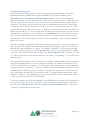
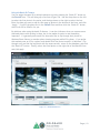
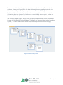
you can choose whether you want your results in decimal days (
) or radians
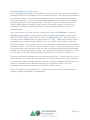
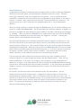
(decimal days*2π). The first step in analyzing your results in R is to convert to radians, so if
you plan on using OVERLAP you might as well export your data in radians and save a step.
In addition to the location filters you have the option to filter your results by date, based on a
hard cutoff (absolute) or date limits relative to the date each camera was set. All of the date
filters are independent, so you can specify an absolute start date with no end date or filter by
both absolute and relative dates. If you specify an absolute end date one day is added so that
photos are excluded starting at midnight the following day (meaning the end date is
inclusive). If you need to specify a date and time for the absolute end date field you should
subtract one day to achieve the correct cutoff. You can also include additional fields if you
like by checking any or all of the boxes in the “Additional Fields” section.
Exporting an activity query is similar to the process for occupancy queries, but the input file
option will create a comma-separated values file (.csv) with the settings in the header. To
import the data from this file into R use the read.csv command and make sure to specify that
the pound sign should be treated as a comment character, otherwise the settings will cause
an error. Your R code should look something like this:
library(overlap)
myData <- read.csv("C:/Users/DoeJ/MyQueryResults.csv",
comment.char = "#")
summary(myData)
spA <- subset(myData, Species == "Red Squirrel")
spB <- subset(myData, Species == "Snowshoe Hare")
spC <- subset(myData, Species == "American Marten")
overlapPlot(spA$Time, spB$Time)
overlapPlot(spA$Time, spC$Time)
overlapPlot(spB$Time, spC$Time)
If you export to a spreadsheet your settings and filters will be added to a separate sheet
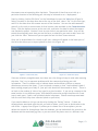
within the workbook. You can also open your query results in a new tab but you can’t save
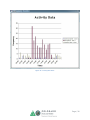
queries built with this form. Instead, you can preview your results in a snappy chart
(Figure 25 - only available when the output format is set to decimal days).
Page | 37