1
HAPTIC SURGICAL AID SYSTEM WITH MAGNETORHEOLOGICAL BRAKES
FOR DENTAL IMPLANTS
By
DORUK SENKAL
A dissertation/thesis submitted in partial fulfillment of
the requirements for the degree of
MASTER OF SCIENCE IN MECHANICAL ENGINEERING
WASHINGTON STATE UNIVERSITY
School of Engineering and Computer Science
DECEMBER 2009
To the Faculty of Washington State University:
The members of the Committee appointed to examine the
dissertation/thesis of DORUK SENKAL find it satisfactory and recommend that
it be accepted.
___________________________________
Hakan Gurocak, Ph.D., Chair
___________________________________
Xiaolin (Linda) Chen, Ph.D.
___________________________________
Wei Xue, Ph.D.
ii
ACKNOWLEDGMENT
I am deeply indepted to Dr. Hakan Gurocak, my thesis advisor, for his valuable
support through my Master’s studies. Not only he helped me through every step of the
research with his supervision and advice, but he also helped me with matters outside the
lab. I believe his guidance will be influential throughout the rest of my career.
I gratefully thank Dr. Ilhan Konukseven, my professor at the Middle East
Technical University, for pointing me in the right direction while I was working for my
Bachelor’s Degree.
I would also like to express my sincere gratitude to Troy Dunmire and Chad
Swanson for machining numerous intricate parts, and their helpful input during the
manufacturing phase of this project.
Finally, my sincere appreciation and thanks are due to my family for their
encouragement and continued support.
iii
HAPTIC SURGICAL AID SYSTEM WITH MAGNETORHEOLOGICAL BRAKES
FOR DENTAL IMPLANTS
Abstract
by Doruk Senkal, M.S.
Washington State University
December 2009
Chair: Hakan Gurocak
This research explored a passive haptic interface as a surgical aid tool for dental
implant surgery. The placement of a dental implant is critical since mistakes can lead to
permanent damage in the nerves controlling the lips, long lasting numbness and failure of the
implant and the crown on it. Haptic feedback to the surgeon in real time can decrease the
dependence on the surgeon’s skills and experience for accurate implant positioning and
increase the overall safety of the procedure. The device developed in this research is a
lightweight mechanism with weight compensation. Rotary magnetorheological (MR)-brakes
were custom designed for this application using the serpentine flux path concept. The resulting
MR Brakes were 33% smaller in diameter than the only commercially available brake yet
produces 2.7 times more torque at 10.9 Nm. Another contribution of the research was a ferrofluidic sealing technique which decreased the off-state torque. A spherical brake as a multiDOF actuator was also developed as a possible candidate for actuation of the wrist joint of the
haptic interface. To the best of our knowledge, our design is the first ever multi-DOF spherical
brake using MR fluid. The control system implemented the passive force manipulability
ellipsoid as an analytical tool for force rendering to follow rigid virtual walls with the passive
device. Usability experiments were conducted to drill holes with haptic feedback. The
maximum average positioning error was 2.88 mm along the x-axis. The errors along the y- and
z-axes were 1.9 mm and 1.16 mm, respectively. The results are on the same order of
magnitude as optical tracking systems and other dental robots, hence passive haptic devices can
be considered a viable alternative to active (servo controlled) haptic devices.
iv
TABLE OF CONTENTS
Page
ACKNOWLEDGEMENTS ............................................................................................. iii
ABSTRACT.................................................................................................................... iv
LIST OF TABLES ........................................................................................................ viii
LIST OF FIGURES ......................................................................................................... ix
CHAPTER
1. INTRODUCTION ................................................................................................ 1
1.1. Passive Haptic Interface ............................................................................... 5
1.1.1. MR Brakes ....................................................................................... 8
1.1.2. Spherical MR Brake ......................................................................... 9
2. PROBLEM STATEMENT AND SCOPE OF RESEARCH ................................ 10
2.1
Development of Compact and Powerful Rotary MR Brakes ....................... 10
2.2
Development of a Spherical MR Brake as a Potential Wrist Mechanism .... 11
2.3
Design of the First Prototype Dental robot.................................................. 12
2.4
Integration with the Virtual Reality Environment and Controller ................ 13
3. MR BRAKES ..................................................................................................... 14
3.1
Rotary MR Brake ....................................................................................... 14
3.1.1 Serpentine Flux Path....................................................................... 15
3.1.2 Ferro-fluidic Sealing ....................................................................... 18
3.2
Spherical MR Brake ................................................................................... 20
3.2.1 Force-feedback Joystick with MR spherical brake .......................... 27
3.2.1.1 Optical Position Measurement System ............................. 28
3.2.1.2 Force Measurement .......................................................... 31
3.2.1.3 Haptic Rendering and Control Architecture ...................... 31
v
4. PASSIVE HAPTIC INTERFACE FOR DENTAL IMPLANT SURGERY ......... 34
4.1
Passive Haptic Interface Design ................................................................. 34
4.2
Balancing ................................................................................................... 34
4.3
Prototype Implementation .......................................................................... 37
4.3.1 End Effector ................................................................................... 39
5. SOFTWARE DEVELOPMENT ......................................................................... 40
5.1
Control System .......................................................................................... 40
5.1.1 High-Level Controller .................................................................... 41
5.1.2 Low-Level Controller ..................................................................... 41
6. EXPERIMENTS AND RESULTS ...................................................................... 13
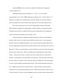
6.1 Rotary MR Brake Experiments ..................................................................... 44
6.1.1 Braking Torque .............................................................................. 45
6.1.2 Wall Collision ................................................................................ 45
6.1.3 Damping Experiment ...................................................................... 49
6.1.4 Coulomb Friction Experiment......................................................... 50
6.1.5 Transient Response ......................................................................... 51
6.1.6 Discussion ...................................................................................... 52
6.2 Spherical MR Brake Experiments ................................................................. 55
6.2.1 Braking Torque .............................................................................. 55
6.2.2 Wall Collision ................................................................................ 56
6.2.3 Transient Response ......................................................................... 58
6.2.4 Damping Simulation ....................................................................... 59
6.2.5 Coulomb Friction Simulation.......................................................... 60
6.2.6 Virtual Environment Simulation ..................................................... 61
6.2.7 Discussion ...................................................................................... 62
6.3
Passive Haptic Interface Experiments ......................................................... 65
vi
6.3.1 Virtual Wall Collision..................................................................... 65
6.3.2 Virtual Wall Following ................................................................... 66
6.3.2.1 Smooth Wall Display ....................................................... 67
6.3.2.2 Unsmooth Wall Display ................................................... 68
6.3.3 Drilling with Haptic Feedback ........................................................ 69
6.3.3.1 Objective .......................................................................... 69
6.3.3.2 Procedure ......................................................................... 69
6.3.3.3 Results ............................................................................. 71
6.3.3.4 Discussion ........................................................................ 72
7. CONCLUSIONS AND FUTURE RECOMMENDATIONS ............................... 74
BIBLIOGRAPHY .......................................................................................................... 77
APPENDIX
A. ASSEMBLY DRAWINGS ................................................................................. 82
B. SOFTWARE ...................................................................................................... 89
C SERVO AMPLIFIER CIRCUITS ..................................................................... 126
D USER MANUAL ............................................................................................. 127
vii
LIST OF TABLES
3.1
Theoretical braking torques for different Spherical MR Brake sizes ..................... 27
4.1
Denavit-Hartenberg parameters for passive haptic arm ......................................... 37
6.1
Results of haptic drilling experiment .................................................................... 71
7.1
Design Specifications of the Prototype MR Brake ................................................ 74
viii
LIST OF FIGURES
1.1
X-Ray image of two dental implants ........................................................................ 1
1.2
Mandibular canal with Mandibular Nerve ................................................................ 2
1.3
Computer milled surgical template and opto-electronic sensors ............................... 3
1.4
Passive Haptic Interface ........................................................................................... 5
1.5
Experiment setup for rotary MR brake ..................................................................... 6
1.6
Spherical MR brake ................................................................................................. 7
3.1
Braking torque in rotary MR brakes ....................................................................... 15
3.2
Serpentine magnetic flux path ................................................................................ 16
3.3
View of serpentine flux path using FEM analysis .................................................. 18
3.4
Ferro-fluidic sealing .............................................................................................. 19
3.5
MR spherical brake flux path ................................................................................. 21
3.6
Calculating cross-sectional area for the forward and return paths ........................... 23
3.7
Magnetic flux density at different azimuth angles .................................................. 24
3.8
Calculating torque about the “x” and “z” axes ........................................................ 25
3.9
Force feedback joystick ......................................................................................... 27
3.10 Optical triangulation system using IR sensors for position measurement ................ 28
3.11 Position and orientation of the optical sensors on the joystick handle ..................... 29
3.12 Control system architecture ................................................................................... 32
4.1
Passive haptic interface .......................................................................................... 34
4.2
Mass balancing ...................................................................................................... 35
4.3
Work volume of the haptic arm.............................................................................. 38
4.4
Handpiece.............................................................................................................. 39
5.1
Haptic arm with the PC Interface and Haptic Rendering ........................................ 40
ix
6.1
Experimental setup for rotary MR brake ................................................................ 44
6.2
Braking torque of rotary MR brake versus current ................................................. 45
6.3
Simulation of collision with a virtual without using the torque sensor. ................... 47
6.4
Simulation of collision with a virtual with the torque sensor .................................. 48
6.5
MR brake as damper in haptics .............................................................................. 49
6.6
MR brake representing Coulomb friction ............................................................... 50
6.7
Transient response and time constant of the MR brake ........................................... 51
6.8
Hysteretic braking torque of spherical MR brake versus current ............................. 55
6.9
Simulation of collision with a virtual wall .............................................................. 58
6.10 Transient response of spherical MR brake .............................................................. 59
6.11 Viscosity simulation with the MR spherical brake as a damper .............................. 60
6.12 Spherical MR brake simulating Coulomb friction along “x” axis ........................... 61
6.13 Virtual environment simulation for a manual gear shifter in an automobile ............ 62
6.14 Collision of the tip with a virtual wall .................................................................... 65
6.15 Smooth wall display .............................................................................................. 68
6.16 Unsmooth wall display .......................................................................................... 68
6.17 Usability experiments ............................................................................................ 70
6.18 Virtual environment for haptic hole placement....................................................... 71
x
CHAPTER 1
INTRODUCTION
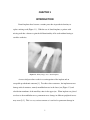
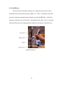
Dental implants have become a routine procedure in prosthetic dentistry to
replace missing teeth (Figure 1.1). With the use of dental implants, a patient with
missing teeth has a chance to gain the full functionality of his teeth without having to
sacrifice aesthetics.
Figure 1.1. X-Ray image of two dental implants.
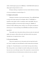
A successful procedure results in osseointegration of the implant and an
acceptable prosthodentic outcome [1]. To achieve these outcomes, the implant must not
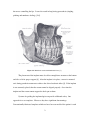
damage critical structures, namely mandibular nerve in the lower jaw (Figure 1.2) and
scheiderian membrane of the maxillary sinus in the upper jaw. When implants are placed
too close to the mandibular nerve, permanent nerve damage in different peripheral nerves
may occur [2, 3]. This is a very serious concern as it can lead to permanent damage in
1
the nerves controlling the lips. It can also result in long lasting paraesthesia (tingling,
pricking and numbness feeling). [2-6].
Figure 1.2. Mandibular canal with Mandibular Nerve [7]
The placement of the implant must also allow enough bone structure at the bottom
and sides of it for proper support [8]. After the implant is in place, a crown is mounted
on it during prosthetic treatment to achieve the desired aesthetic affect [9]. If the implant
is not accurately placed, then the crown cannot be aligned properly. Over time the
implant and the crown cannot support the loads put on them.
Systems for guiding the implantologist can provide additional safety. One
approach is to use templates. However, they have significant shortcomings.
Conventionally fabricated templates which are based on wax model of the patient’s teeth
2
structure do not take the thickness of the mucosa, topography of the underlying bone or
vital anatomical structures into consideration. In addition, limitations of current
fabrication techniques do not allow fabrication of a template that remains stable during
surgery [10]. Hence, they can only be used to optimize the position of the implants for
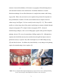
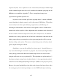
later prosthodontics treatment. For this reason methods that use templates based on
volume image data (Figure 1.3a) have recently been developed [11, 12]. These methods
usually use volume image data of the patient’s underlying jaw structure-obtained through
computer tomography (CT) or digital volume tomography (DVT). Advanced
manufacturing techniques, such as stereo-lithography, together with specialized implant
planning software [13] are used to manufacture drilling templates [14]. Although these
templates take the hidden anatomy into consideration and significant improvement in
placement accuracy is reported, they suffer from high costs of CAD/CAM processing
[15] and added lead time. In addition, they lack flexibility, as any change in the planning
requires the manufacturing of new templates [8].
(a)
(b)
Figure 1.3. (a) Computer milled surgical template [14]. (b) Opto-electronic sensors with light emitting
diodes on the hand-piece with Graphical User Interface of the system [16].
3
Another method for implant placement uses Image Guidance Implantology
systems (IGI) [17, 18]. These systems use optical sensors with light emitting diodes
(Figure 1.3b), attached to the hand-piece of the drill and to the patient to track their
relative positions. Combining this information with the volume data of the patient’s jaw
structure makes it possible to view the preoperative planning together with the drill
position in real-time. Using these systems intra-operative safety can be increased as
critical anatomic structures such as nerves can be avoided with the aid of the graphical
user interface from the system [16]. However, even with the help of the graphical user
interface, it is difficult to achieve proper position and angulation as random factors such
as trembling cannot be eliminated without the guidance of a mechanical system. Errors
as high as 1.23 ± 0.28 mm on average and a maximum of 1.87 ± 0.47 mm between the
planned position of the fiducial point marker have been reported [19]. For this reason,
the quality of the intervention is still largely dependent on the surgeon’s skills and
experience [1].
A surgical robot system for maxillofacial surgery [20] has been developed. With
this system the surgeon interactively programs the robot during the surgery after which
the robot performs the pre-programmed tasks. A haptic system for bone drilling has also
been developed [21]. This system uses a PHANToM Haptic Device [22] for “virtual”
bone drilling. The system was intended for training and not for actual surgery. The
average misalignment was reported to be less than 0.2 mm, indicating that the system is
potentially applicable to oral implant surgery. A robotic assistant for dental implantology
was built which used a robot arm and CT scans to hold a drill guide over a phantom jaw
[23, 24]. Deviations of approximately 1 to 2 mm were obtained using this system.
4
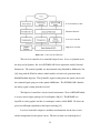
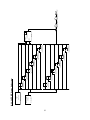
1.1 Passive Haptic Interface
Due to the complexity of the anatomic structure and the procedure, a surgical aid
system for dental implants is highly desirable to ensure the success of the procedure.
Such a system can decrease the dependence on surgeon’s skills and experience for
implant position accuracy, and increase the overall safety of the procedure. The system
would track the surgeon’s hand-piece and the patient to provide graphical user interface
and haptic feedback to the surgeon in real time to guide him during the operation.
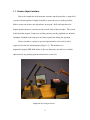
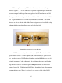
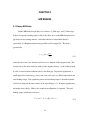
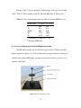
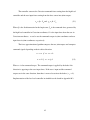
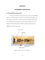
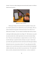
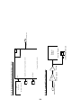
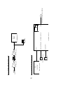
In this research we explored a passive haptic interface to be used in such a
surgical aid system for dental implants (Figure 1.4). The interface uses
magnetorheological (MR) fluid brakes as they are inherently safe and have excellent
characteristics in providing rigid interaction forces to the user.
Figure 1.4. Passive Haptic Interface
5
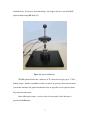
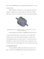
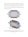
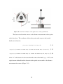
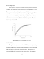
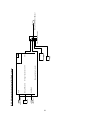
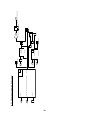
We developed a new rotary MR brake as the actuator for the dental haptic
interface (Figure 1.5). The new brake uses a serpentine magnetic flux path which leads
to a more compact brake design. Our prototype brake has 63.5 mm diameter and 10.9
Nm torque at 1.5 A current input. Another contribution of the research is a ferro-fluidic
seal. In general, MR brakes use O-rings to prevent leakage of the fluid. The O-Ring
increases the off-state friction of the brake. In our design we used a ferro-fluidic sealing
technique which reduced the off-state torque and sealed the fluid.
Figure 1.5. Experiment setup for rotary MR brake
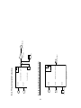
All MR actuators are single degree-of-freedom (DOF). The wrist joint of the
passive haptic interface is a 3 DOF spherical joint, with individual yaw, pitch and roll
axis. In order to create a 3-DOF spherical joint three rotational MR brakes are needed in
a gimbal arrangement. In this configuration, the resulting mechanism is usually rather
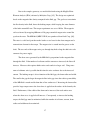
large. In this research we explored design of a MR spherical brake as a multi-DOF
actuator (Figure 1.6). Unlike the single-DOF brakes, the spherical brake allows motion
about any arbitrary axes. When it is activated, it can restrict or lock all three DOFs
6
simultaneously. To the best of our knowledge, our design is the first ever multi-DOF
spherical brake using MR fluid [25].
Figure 1.6. Spherical MR brake
The MR spherical brake has a diameter of 76.2 mm and can apply up to 3.7 Nm
braking torque. Another contribution of the research is an optical position measurement
system that eliminates the gimbal mechanisms that are typically used in spherical joints
for position measurement.
In the following sections, a review of the relevant studies in the literature is
provided for MR Brakes.
7
1.1.1 MR Brakes
MR brakes create braking torque by changing the viscosity of the MR fluid inside
the brake. In the inactive state the fluid has a viscosity similar to low-viscosity oil. Upon
activation with a magnetic flux, it changes to a thick consistency similar to peanut butter.
MR brakes are used in many applications including prosthetics, automotive, vibration
stabilization and haptics.
The MR brakes provide quick response with simple control. When used alone or
in combination with motors, MR brakes have been shown to provide realistic rigid virtual
object simulations in haptics applications [26-29]. However, to obtain significant braking
forces/torques, the brakes are required to be rather large and use high input current.
There is a commercially available MR brake by Lord Corporation [30]. This brake
(model RD-2087-01) has 96.6 mm diameter, 43.7 mm width and can provide 4 Nm
torque with 1.5 A current input. An MR brake was designed as a clutch for automotive
applications [31]. The clutch had 152 mm diameter and required 4 A to generate a
braking torque of 6.9 Nm. A single-disk MR brake was designed for haptic rendering
[32]. The brake had a diameter of about 80 mm. It was smaller than some of the other
examples in literature but could only provide 1.4 Nm torque in spite of the 4 A input
current. Another single-disk MR brake with about 130 mm diameter was designed and
experimentally tested [33]. This brake provided 1.4 Nm maximum braking torque at
0.75 A input current. To improve the performance of MR brakes a design optimization
method using Finite Element Analysis was proposed [34]. The method resulted in 25%
height reduction leading to a brake with 120 mm diameter and 38 mm height. At 5 A
input current the brake provided 4.25 Nm torque output.
8
1.1.2 Spherical MR Brake
A two-DOF joystick was developed for haptics applications [35]. The design
integrated two one-DOF MR disc brakes into a joystick using a gimbal mechanism. The
MR disc brakes had 78 mm diameter. The overall prototype joystick had a base of about
160 mm × 160 mm and provided up to 10 Nm braking force to the joystick handle.
Another multi-DOF device was designed using two groups of MR actuators to simulate
virtual forces in 2D [36]. The system used four MR rotary brakes each with 170 mm
diameter and 10 mm height. The overall system size was 630 mm × 540 mm × 970 mm.
The maximum output torque on the handle was 10 Nm. Two other multi-DOF devices
were reported that used electrorheological (ER) fluids. The first device used both clutch
and brake mechanisms to achieve active and passive force feedback [37]. The device
integrated four AC motors with a spherical ER joint at the center. The spherical joint
assembly had an estimated diameter of 110 mm. When the motors were included, the
system took up about 45 cm × 45 cm area. A complex controller was implemented
resulting in about 7 N force output on the joystick handle from the spherical joint. The
second device consisted of a metal sphere which was concentrically mounted in a metal
half sphere [38]. The gap between them was filled with ER fluid. The spherical joint had
102 mm diameter. At 2.8 kV/mm electric field strength, the device produced 1.2 Nm
output torque.
9
CHAPTER 2
PROBLEM STATEMENT AND SCOPE OF RESEARCH
The long term goal is to develop a dental robot to assist in oral implant surgery.
Development of a first prototype robot as an initial step towards this goal is the basis of
this research. The objective is to design a lightweight robot with passive actuators to
assess the advantages and limitations of such a design. The research contains four
phases:
2.1 Development of Compact and Powerful Rotary MR Brakes
A dental robot that would be placed in a dentist‘s office needs to be lightweight
and strong, as the surgeon already needs to work in a very limited work volume such as
the patient’s mouth cavity. Actuators are one of the primary components that affect the
size of a robot arm. Traditionally, DC-motors are used for controlling a haptic arm.
However DC-motors usually have rather small torque-to-size ratios. For that reason,
either very large motors need to be used or a very high reduction ratio needs to be
employed by using transmission mechanisms such as gears or pulleys. The transmission
elements add to the overall robot size as well as unwanted effects such as backlash,
deflection or slippage. As MR brakes usually have several orders of magnitude higher
torque to size ratios than DC-motors, a design that uses MR brakes with direct coupling
to the joint axis was chosen for the haptic interface.
To the best of our knowledge, there is only one commercially available rotary MR
brake in the market [31]. Although this brake provides comparably higher torque to same
10
sized DC-motors, it is a disc-type MR brake, along with many other MR brakes in the
literature. In this research we explored the design of new type of brake based on
serpentine flux path concept. Using this method we aimed to build compact yet high
torque drum-type MR brakes.
Another contribution of this research was in sealing of MR fluid inside the MR
brakes. Traditionally rubber seals are used to keep the MR fluid from leaking out.
Although this is a perfectly viable method for MR brakes that are used in applications
such as exercise equipment or automobile clutches, the friction created by such a sealing
method is highly undesirable in haptics applications. Any unwanted off-state friction
would reduce the back-drivability of the haptic device, effectively decreasing the realism
of the haptic feedback. In this reaserch we explored an alternative sealing method called
ferro-fluidic sealing. Ferro-fluidic seals are normally used for sealing the lubricants
inside rotating assemblies like gearboxes, bearings etc. By placing permanent ring
magnets at the two ends of the rotor shaft, we aimed to solidify the MR fluid inside the
end-caps and hence prevent rest of the fluid from leaking out.
2.2 Development of a Spherical MR Brake as a Potential Wrist Mechanism
In this first prototype, the commonly used pen-based haptic devices [21] were
taken as the basis. Hence, three joints were actuated with MR-brakes for creating the
haptic feedback and the remaining three joints at the wrist were left un-actuated to
provide motion in 6 DOF. In essence when the MR brakes are activated, the position of
the base of the hand-piece is constrained, whereas the orientation of the hand-piece is not.
In the future prototypes, the last 3 DOF need to be actuated if orientation also needs to be
11
constrained. This can be accomplished by using smaller MR brakes at the wrist.
However since rotary MR brakes are 1 DOF devices, a gimbal mechanism need to be
employed with 3 rotary MR brakes to create the spherical joint at the wrist. We explored
another alternative, by designing a spherical MR brake. The spherical brake allows
motion about any arbitrary axes. When it is activated, it restricts motion around all three
DOFs simultaneously. To the best of our knowledge, this is the first ever multi-DOF
spherical brake using MR fluid.
2.3 Design of the First Prototype Dental Robot
Our primary design goal is to provide haptic feedback to the surgeon through the
hand-piece. Such a system does not have the usual master-slave relationship of a
teleoperated system. In this case, they are collocated since the surgeon uses the handpiece as he/she normally would and haptic feedback is added to it. By eliminating the
need for a programmable robotic manipulator we aimed to obtain a high level of
transparency, which is much desired in surgical procedures.
For such a system to be useful in a dental implant surgery the system must be
lightweight. As the surgeon has to work inside the patient‘s mouth cavity, he/she has
very limited reach. A bulky design would seriously deteriorate the surgeon’s
performance. The system must also be safe. Due to the nature of the operation, any
malfunction in the surgical aid system might result in catastrophic results.
With these design requirements in mind, a passive haptic interface with MRbrakes has been designed. The MR-brakes have very high torque-to-size ratio [25, 39,
40], hence they are a very good choice for a lightweight design. Since MR-brakes are
12
passive devices they are inherently safe. They cannot add energy into the system, but can
only dissipate it. They have excellent wall collision characteristics enabling near rigid
interaction forces to be delivered to the hand-piece. They do not require sophisticated
controllers.
2.4 Integration with the virtual reality environment and controller
As in other pen-based haptic devices, the user interacts with the virtual
environment by grasping the hand-piece and moving it. The base of the hand-piece
(center of the gimbal mechanism at the wrist joint) is represented by a point in the virtual
environment. The device creates the haptic feedback by selectively locking the MR
brakes. The resulting resistance forces are used to render virtual surfaces.
As MR brakes can only apply forces opposing the user’s motion, traditional
control algorithms for haptics cannot be used for the control of MR-brakes. For this
reason a two-tiered control algorithm has been implemented in this research. First,
required output forces based on the position of the haptic arm are calculated using a
penalty based haptic renderer [41, 42]. Later these command forces are passed through a
force approximation algorithm to create the closest force output that can be obtained by
using MR brakes [43, 44]. This way haptic feedback of tasks such as wall following
could be approximated.
13
CHAPTER 3
MR BRAKES
3.1 Rotary MR Brake
Rotary MR brake designs have two varieties: (1) Disk type, and (2) Drum type.
In these designs the braking torque is due to the shear stress of the MR fluid placed in a
gap between two rotating surfaces. Often the behavior of controllable fluids is
represented as a Bingham plastic having variable yield strength [33]. The flow is
governed by:
τ = τ yd ( B ) + η
ω⋅r
h
(3.1)
where the first term is the dynamic yield stress as a function of the magnetic flux. The
second term is the shear strain rate with ω is the angular velocity, r is the radial position,
η is the viscous friction coefficient and h is the fluid gap. In practical applications, a
small torque due to friction (e.g. due to the seals) also exists as a third component in the
total braking torque. The significant portion of the braking torque is from the dynamic
yield stress acting on the outer surface of the rotor (Figure 3.1). In haptics applications,
the brakes rotate slowly. Hence, the second term in Equation 1 is ignored. The total
braking torque can then be written as:
T = 2π ⋅ r 2 ⋅ L ⋅ τ yd ( B ) + TCoulomb
14
(3.2)
where τyd(B) is the MR fluid shear stress as a function of magnetic flux and TCoulomb is the
mechanical friction.
While the MR brakes are widely used in a variety of applications from exercise
equipment to automobiles they are usually too bulky to be effectively used in haptics
applications. Also, the off-state friction is an issue in their usage in haptics applications.
Figure 3.1. Braking torque in rotary MR brakes is a function of the dynamic shear stress on the rotor
controlled by the magnetic flux.
In the existing designs only a limited area of MR fluid in the gap can be kept at
the required magnetic field strength to activate the fluid. Also, since magnetic field
strength is more or less inversely proportional to flux path cross-sectional area, the
maximum MR fluid gap that can be actuated is limited. As a result, the only options to
obtain high levels of torque are to increase the brake radius, coil windings and current.
All of these options lead to a bulky design due to the size of the coil and the disk or drum.
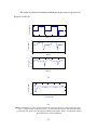
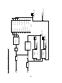
3.1.1 Serpentine Flux Path
To design an MR brake with higher torque without increasing the size of the
brake, more surface area of the MR fluid must be activated by the magnetic flux. We
15
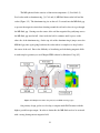
achieved this by creating a serpentine flux path. By strategically placing magnetically
conductive 1018 steel rings and non-conductive Aluminum rings it is possible to bend the
magnetic field and weave it through the MR fluid gap multiple times (Figure 3.2). This
led to a more compact brake design and enabled us to increase the braking torque without
increasing the size of the brake.
Bobbin wire
MR fluid gap
Figure 3.2. Serpentine magnetic flux path weaving through the drum and the outer shell (top). It enables
activation of more of the MR fluid for increased braking torque. MR fluid between the outer shell and
the rotor with the coil (bottom).
16
Due to the complex geometry, we modeled the brake using the MagNet Finite
Element Analysis (FEA) software by Infolytica Corp. [45]. The design was optimized
based on the magnetic flux density computed in the fluid gap. The goal was to maximize
the flux density in the fluid, hence the braking torque, while keeping the outer diameter
of the brake around 65 mm. The torque requirement was set at 10 Nm. The magnetic
coil was formed by wrapping 800 turns of 26-gauge enameled magnet wire around the
spool on the rotor. The MR fluid (MRF-132LD) was purchased from Lord Corp. [46].
The rotor is a solid steel part that works both as a steel core for the electromagnet and a
transmission element for the torque. The magnet wire is wound into the groove on the
shaft. The two ends of the magnet wire pass through tiny holes along the shaft axis to be
connected to power supply.
The shear stress generated by the MR fluid is proportional to the magnetic flux
through the fluid. If the number of coil turns and the current are increased, the flux will
increase. However, this requires thicker wires and results in a larger coil. Using more
turns of a thinner wire is possible but this time the wire overheats due to the increased
current. The braking torque is also a function of the fluid gap, the drum radius and width.
The smaller the gap the larger the magnetic flux in the gap since the relative permeability
of the MR fluid is much smaller than that of low-carbon steel. Increasing the drum radius
provides larger torque arm as the shear force is applied on the surface of the drum by the
fluid. Furthermore, if the width of the drum can be increased, the total surface area
where the shear stress is applied will increase. Consequently, to increase the braking
torque, the fluid gap must be minimized while the number of coil turns, current, drum
radius and width must be maximized.
17
After much iteration, the optimal design had a rotor with 52 mm radius, 47 mm
length and 0.25 mm fluid gap producing an average of 1.03 Tesla flux in the MR fluid
(Figure 3.3). Based on the manufacturer’s specifications for the MRF-132LD fluid, the
shear stress corresponding to the 1.03 Tesla flux was 55 kPa [46]. With these dimensions
and the shear stress value, the maximum braking torque output for an input of 1.5A
current was calculated as 10.83 Nm using equation 2. The Coulomb friction was ignored
since the design incorporates ball bearings reducing the mechanical friction between the
shaft and its housing down to negligible levels. This assumption was later validated in
experiments.
Figure 3.3. Quarter sectional view of the MR-Brake showing the serpentine magnetic flux using FEM
analysis.
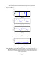
3.1.2 Ferro-fluidic Sealing
MR brakes usually employ an O-ring between the rotor and stator to seal the fluid
in. Although this is an effective mechanism to prevent fluid leakage, the O-Rings
increase the off-state friction of the MR brake. The off-state friction is an important
parameter for haptic applications. Furthermore, the MR fluid has been shown to be very
18
abrasive on the O-rings. In this research, we developed a novel sealing approach using
ferro-fluidic sealing assemblies on both sides of the brake shaft (Figure 3.4). The ferrofluidic sealing assemblies have three primary roles in the brake assembly: (1) Prevent the
leakage of the MR fluid, (2) hold the roller bearings necessary to keep the shaft in place,
and (3) connect the chassis to a stationary point via aluminum flanges.
Bearing
Magnet ring
Magnet ring
Flux path
Ferrofluidic Seal
Brake shaft
Ferrofluidic seal
Steel casing
Air gap
Figure 3.4. Ferro-fluidic sealing using a ring magnet (left). Ball bearing supports the rotor. Crosssectional view of the ferro-fluidic seal and the flux path (right).
These ferro-fluidic seals work by using the MR fluid itself as a sealing element.
Circular magnets placed at both ends produce magnetic flux paths that cross the gap
between the shaft and the chassis (Figure 3.4). The magnetic field increases the yield
stress of the MR fluid inside the gap, which builds a pressure differential that keeps the
MR fluid from leaking out. As there is no active contact between solid bodies this
approach helps decrease the off-state friction tremendously which is critical in haptic
displays.
19
3.2 Spherical MR Brake
Devices that use MR fluids have several advantages over devices with ER fluids.
Yield shear stress of MR fluids is much higher than ER fluids, this leads to higher torque
output. The ER fluids require potential differences as high as 3 kV in order to be
activated, whereas devices that use MR fluids have much lower voltage requirements
usually in the range of a few volts. This becomes even more important if the device is to
be used in environments, such as haptics, where human interaction will be present.
Failure in a 3 kV circuit can be very dangerous to the user.
A big challenge in designing devices that use MR fluids is routing the magnetic
flux path through the fluid while keeping the overall device size compact and the output
torque high. Both in ER and MR fluids the fields that are applied to the fluid must be
perpendicular to the fluid gap. This requirement is satisfied easily with ER devices as
applying a potential difference between any two surfaces would automatically create
electric fields perpendicular to those two surfaces hence also perpendicular to the ER
fluid in the gap. With MR brakes it is more difficult since a coil for an electromagnet
must be housed in the brake and the resulting flux path must be guided through the fluid
by carefully designing the magnetic circuit.
Previously we designed single DOF rotary, compact and powerful MR brakes
using a serpentine flux path concept [39, 40]. In this approach, aluminum and steel rings
were employed to weave the magnetic flux path through the MR fluid gap. This led to
activation of much more of the MR fluid in the same compact volume. The same concept
was adapted in the design of the MR spherical brake.
20
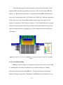
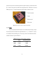
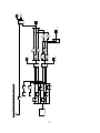
The MR spherical brake consists of four main components: (1) Steel ball, (2)
Steel socket with an aluminum ring, (3) Coil, and (4) MR fluid between the ball and the
socket (Figure 3.5). The aluminum ring sits on the coil. It extends into the MR fluid gap
to prevent the magnetic circuit from shorting around the coil and to force it to go through
the MR fluid gap. Starting near the center of the coil the magnetic flux path jumps across
the MR fluid gap into the ball. Once inside the ball, it continues until it passes to the
other side of the aluminum ring. On the top side of the aluminum ring it jumps across the
MR fluid gap once again going back into the socket where it completes its loop back to
the center of the coil. Due to the difficulty of visualizing and calculating magnetic fields
in such complex geometry we used Magnet FEM software by Infolytica Corp. [45].
Figure 3.5. MR Spherical brake flux path (left) and FEM modeling (right).
Our primary design goal was to develop a compact multi-DOF actuator with the
highest possible torque output. In order to obtain this, the MR fluid needs to be activated
with a strong, homogeneous magnetic field.
21
The size of the magnetically conductive parts was one of the parameters
conflicting with this requirement since reducing the cross-sectional area along the path of
the magnetic circuit has a negative effect on the amount of magnetic flux that can pass
through it. This phenomenon is also known as core saturation because the magnetic flux
density in a magnetic circuit is ultimately limited by the saturation point of the magnetic
material being used.
Another parameter that needed to be optimized was the homogeneity of the
magnetic field across the MR fluid gap. For our design, we aimed at obtaining 1 Tesla
throughout the MR fluid, which, according to manufacturer’s specifications, is very close
to the saturation point of the MR fluid (MRF-132LD from Lord Corp.) [46]. This helped
make maximum use of the MR fluid in the gap but it also required design of a wellbalanced magnetic circuit. An unbalanced magnetic circuit would cause the fluid to
saturate in one part of the brake while leading to insufficient magnetic flux densities at
other points. For this reason, the position of the aluminum ring along the MR fluid gap
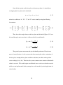
circumference is critical as it divides the surface area of the MR fluid gap to forward and
return paths (Figure 3.6) which determine the ratio of magnetic flux density along these
two surfaces. The magnetic flux Φ is the same at any point along the magnetic circuit:
Φ = Φ
(3.3)
In terms of magnetic flux density “B” and the surface area “A” through which the
flux flows, the same equation can be written as:
∙ = ∙ 22
(3.4)
The ring must be placed at a location where the resulting surface areas on both the
forward and return flux paths will allow equal flux densities on both sides. In other
words, the forward and return cross-sectional areas need to be equal. To find the location
of the aluminum ring the areas were computed as:
Figure 3.6. Calculating cross-sectional area for the forward and return paths.
2 ∙ ∙ sin ∙ = 2 ∙ ∙ sin ∙ (3.5)
2 − cos !"| = 2 − cos !"|
(3.6)
$ = cos%& '
&()*+ ,
(3.7)
where $ is the angle at which the aluminum ring is placed, - is the angle where the MR
Fluid gap ends and “r” is the radius of the sphere. Increasing - has a positive effect on
the torque output because of the increased MR fluid gap area, but at the same time it is a
limiting factor for the spherical MR Brake’s work volume since it reduces the motion
23
range of the handle attached to the ball. For this reason, first a moderate socket size of
- = 120 was selected. Then, $ = 75.5 was computed as the location for the
aluminum ring. Accuracy of this method was also verified using FEM. Thirteen data
points inside the MR Fluid gap were taken (Figure 3.7). At 1.5 Amps 1.14 ± 0.02 Tesla
was found throughout the MR Fluid gap. The flux density in the gap is fairly uniform as
a result of the strategic placement of the aluminum ring.
Figure 3.7. Magnetic flux density at different azimuth angles.
MR spherical brake can exert moments along all 3 axes, hence maximum torque
along each axis should be individually calculated. This is accomplished by integrating
the tangential component of yield stress along the ball surface for each axis. It should be
noted that because of the symmetry along “z” axis, maximum torque that can be exerted
along “x” and “y” axes will be equal.
24
Figure 3.8. Calculating torque about the “x” and “z” axes. is the azimuth angle, φ is in the horizontal
x-y plane.
Torque about the z-axis can be calculated by integrating shear stress on the sphere
from = 0 to = - (Figure 3.8). By taking advantage of the symmetry along the z-
axis, the moment arm can be written as: ∙ sin and the shear force on an infinitesimally
thick ring around the sphere can be written as: 3 ∙ 2 ∙ sin ∙ . Then the integral
becomes:
7
56 = ∙ sin ! ∙ 3 ∙ 2 ∙ ∙ sin !
7
9
+:; 9
56 = 3 ∙ 2 ∙ 8 ∙ "' − < ,=
(3.8)
(3.9)
Using a similar approach torque along the “x” and “y” axes can be
calculated. However the absence of symmetry along the “x”-axis makes it impossible to
use the above equation directly. Instead, the torque that can be created by the surface
25
area of the opening on the socket is subtracted from the torque that can be created by a
complete sphere:
5>,@ = 5ABCD
− 5CEF
(3.10)
5ABCD
can be calculated by using equation 8 with - = to cover the whole
surface area of the sphere:
5ABCD
= 3 ∙ ∙ 8
(3.11)
The torque that needs to be subtracted due to the opening can be calculated by a
double integration over the opening. The moment arm can be written as:
G ∙ cos ! + ∙ sin ∙ sin I! and shear stress at any point on the opening can be
written as: 3 ∙ ∙ sin ∙ I ∙ . Then, the double integral for the opening becomes:
J%7
5CEF = J
2 3 ∙ 8 ∙ sin ∙ Gcos ! + sin ∙ sin I! ∙ I ∙ (3.12)
Substituting into equation 9 gives:
J%7
5>,@ = 3 ∙ ∙ 8 − J
2 3 ∙ 8 ∙ sin ∙ Gcos ! + sin ∙ sin I! ∙ I ∙ (3.13)
For = 20.32LL and 3@ 1 5MNOP! = 55QRP for the fluid we used, the torque
values that can be exerted by the MR Spherical Brake are found as 56 = 3.66TL and
5>,@ = 3.28T. L .
26
Because of the 8 term in equation 12, braking torque scales up very well with
radius. Table 3.1 shows braking torques for spherical MR brakes at different sizes.
Table 3.1: Theoretical braking torques for different spherical MR brake sizes
Radius (mm)1
5
10
20.322
30
50
1
2
Tz (N.m)
0.06
0.44
3.66
11.79
54.59
Tx,y (N.m)
0.05
0.39
3.28
10.54
48.82
: Calculations are done at - = 120°
: Prototype MR Brake
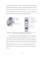
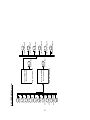
3.2.1 Force-feedback joystick with MR spherical brake
The MR spherical brake was used in the design of a force feedback joystick for
haptics applications (Figure 3.9). The joystick handle, equipped with force sensing, was
attached to the spherical MR-brake. An optical position measurement system was also
attached to the handle.
Figure 3.9. Force feedback joystick.
27
3.2.1.1 Optical Position Measurement System
Conventional spherical joints use encoders attached to three different axes of the
joint through a gimbal mechanism to measure the orientation [47]. Although this is a
viable approach, we explored another approach to meet the design goal of building a
compact system.
Three IR sensors by Sharp, Inc. were used to build an optical triangulation system
to measure the position of the joystick handle (Figure 3.10).
Figure 3.10. Optical triangulation system using IR sensors for position measurement.
The sensors measure distance by sending an infrared signal and receiving the
signal that bounces back from a surface. They have a range of 4 to 30 cm and generate
an analog signal corresponding to the measured distance. The sensors were placed in a
triangular arrangement angled slightly outward and facing down.
28
Figure 3.11. Position and orientation of the optical sensors on the joystick handle.
The data received from the sensors are the distance measurements to three points
on the base plane. The coordinates of these three points with respect to the joystick
handle can be found as:
W& , X& , Y& ! = Z + sin [ ∙ & , 0 , cos [ ∙ & !
W , X , Y ! = −cos 60° ∙ Z −cos 60° ∙ sin [ ∙ , sin 60° ∙ Z + sin 60° ∙ sin [ ∙ , cos [ ∙ !
(3.14)
(3.15)
W8 , X8 , Y8 ! = −cos 60° ∙ Z −cos 60° ∙ sin [ ∙ 8 , −sin 60° ∙ Z −sin 60° ∙ sin [ ∙ 8 , cos [ ∙ 8 ! (3.16)
where "Z" is the distance of each sensor from the centre of the handle, [ ([ = 30°) is the
angle between the handle and the direction of the optical sensors and is the distance
measurement for sensor ] (Figure 3.11).
29
Once the three points on the base plate are known, position of a virtual plane
overlapping the base plate can be calculated:
∙W+∙X+^∙Y+_ = 0
(3.17)
where the coefficients “A”, “B”, “C” and “D” can be found by using the following
determinants:
1
= `1
1
X&
X
X8
Y&
W&
Y ` = `W
W8
Y8
1 Y&
W&
1 Y ` ^ = `W
1 Y8
W8
X&
X
X8
W&
1
1` _ = − `W
W8
1
X&
X
X8
Y&
Y ` (3.18)
Y8
Then, the relative angles between the base plate and the handle (Figure 3.12) can
be found through a unit vector that is collinear with the joystick handle:
%b
,
(3.19)
%d
,
(3.20)
a> = sin%& '√de
(b e(f e
a@ = sin%& '√de
(b e (f e
The optical system can measure the joystick handle position in 3D as the user
moves it in any direction. As the system works by measuring the relative orientation of
the base plate, rotating the base plate would have absolutely no effect on the position
sensor readings d& , d , d8 !. Therefore, the system cannot measure rotation of the handle
about its own axis. This would require an additional sensor, such as an absolute encoder,
which was not implemented in this prototype due to the intended joystick application for
virtual reality.
30
3.2.1.2 Force Measurement
When passive actuators, like the MR spherical brake, are used in haptics
applications, it is necessary to measure the forces applied by the user in addition to
position measurements to control the behavior of the device. If only position is
measured, then the so called “sticky wall” [48] situation occurs where the joystick will
not release the brake as the user tries to pull away from a collision with a virtual object.
We built a simple load cell with two sets of strain gage full bridges to measure the
forces applied by the user on the handle. Although the spherical MR-brake is able to
generate moments in all three DOF, in this study we concentrated only on measurement
of the user forces in “x” and “y” directions. For the intended purpose of the prototype as
a haptic joystick the moment around the handle was neglected since it was not needed.
The load cell was made of aluminum and its design was optimized using finite element
analysis. The strain gages were connected to strain gage amplifiers (5B38-05) by Analog
Devices. The circuitry was interfaced to a data acquisition card (PCI-MIO-16E-4) by
National Instruments.
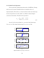
3.2.1.3 Haptic Rendering and Control Architecture
Virtual environments integrated with haptic devices typically run two processes.
The first process involves collision detection, haptic rendering and updating the graphics
in the virtual world with about 15-30 frames per second. The second process is the
control loop of the haptic device which usually runs at 1000 Hz. As shown in Figure
3.12, we implemented a two-layer control architecture consisting of a low-level and highlevel controller.
31
Force-feedback joystick
Hardware Interface
Low-level controller
High-level controller
Figure 3.12. Control system architecture.
The low-level controller is to control the haptic device. It uses a Q4 hardware-inthe-loop card by Quanser, Inc. and a PCI-MIO-16E-4 data acquisition card by National
Instruments. The control algorithm was implemented using Simulink by Mathworks, Inc.
[49] along with the WinCon software which enables real-time code generation from
Matlab/Simulink diagrams. The Q4 handles signals coming from the optical sensors and
the command signal going out to the spherical MR-brake. The PCI-MIO-16E-4 handles
the analog signals coming from the load-cell.
The high-level controller is for the virtual environment. We used H3DAPI which
is an open source haptics package by SenseGraphics AB [41]. The H3DAPI uses
OpenGL to render graphics and has its own haptics renderer called HAPI. We chose the
proxy-based Ruspini algorithm for the haptic rendering [42].
Low-level controller computes coordinate transformations for the force sensor
and the triangulation for the optical sensors. The data are then sent to the high-level
32
controller which generates the command force necessary to create the haptic sensation.
The command force is returned to the low-level controller which processed the command
signal and the force input from the user to compute the necessary braking torque signals.
This signal then goes to the spherical MR-brake through a current-controlled servo
amplifier. Details and implementation of the controller for the spherical MR brake can be
found in Appendix B.1 along with the Simulink/H3DAPI interface code in Appendix B.3.
33
CHAPTER 4
PASSIVE HAPTIC INTERFACE FOR DENTAL IMPLANT SURGERY
4.1 Passive Haptic Interface Design
The prototype consists of four components: (1) MR-brakes (2) Position sensors
(3) A 6-DOF force sensor and (4) Hand-piece for drilling (Figure 4.1). Pen-based haptic
devices [22] were taken as an example in the design of this first prototype. Hence, three
joints were actuated with MR-brakes for creating the haptic feedback and the remaining
three joints were left un-actuated at its wrist to provide motion in 6 DOF. CAD drawings
of the passive haptic interface can be found in Appendix A.
Figure 4.1. Passive haptic interface
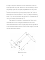
4.2 Balancing
The weight of the arm should not be felt by the surgeon to ensure transparency of
the system. Therefore, the arm was made out of lightweight components. Furthermore,
34
its weight was compensated. Since there are no active actuators in the system active
weight compensation is not possible. For this reason, static mass balancing was done by
using balancing weights and by strategically placing MR-brakes on the arm geometry.
The brakes were positioned close to the center of rotation of joints 2 and 3 in order to
minimize the inertia of the system (Figure 4.2). Brake 3 (at J3) together with balancing
weight “A” (݉ ) were used to balance the arm around joint 2 (J2). Balancing weight “B”
(݉ ) was used to balance the arm around joint 3 (J3).
Torque applied to J4 is transferred to J3 by mechanical links. Hence, it can be
assumed that joints J4 and J3 are overlapping and the link between ݉ and ݉ଶ is
connected to the link between ݉ସ and ݉ . Using this principle, the only weight that tries
to rotate the arm in the clockwise direction is m6. The rest of the weights try to rotate the
arm in the counter-clockwise direction.
Figure 4.2. Mass balancing
35
Since the weight of the hand-piece is relatively small mass balancing around the
un-actuated joints J4, J5 and J6 was neglected. Also, as the first joint axis is in the
direction of gravity, only joints 2 and 3 need to be balanced. The weight of the linkages
is transferred equally to the joints they are attached. Therefore, mass balancing can be
done by considering the joints as point masses.
For J3:
݀ ⋅ ݉ + ݀ଷ ⋅ ሺ݉ଷ + ݉ସ ሻ ⋅ cosሺߨ − ߚ ሻ = ሺ݀ ⋅ ݉ ሻ ⋅ cosሺߨ − ߚ ሻ
(4.1)
cosሺߨ − ߚ ሻ terms cancel out giving:
݀ ⋅ ݉ + ݀ଷ ⋅ ሺ݉ଷ + ݉ସ ሻ = ሺ݀ ⋅ ݉ ሻ
(4.2)
Since no position variables remain in equation 4.2, J3 can be statically balanced.
Similarly, for J2:
ሺ݀ଶ ⋅ ݉ଶ + ݀ ⋅ ݉ ሻ ⋅ cosሺߠሻ + ሺ݀ଶ ⋅ cosሺߠሻ + ݀ଷ ⋅ cosሺߨ − ߚ ሻሻ ⋅ ݉ଷ
+ ሺ݀ଶ ⋅ cosሺߠሻ + ݀ ⋅ cosሺߨ − ߚ ሻሻ ⋅ ݉ = ሺ݀ହ ⋅ cosሺߠሻሻ ⋅ ݉ହ
(4.3)
+ሺ݀ହ ⋅ cosሺߠሻ − ݀ଷ ⋅ cosሺߨ − ߚ ሻሻ ⋅ ݉ସ + ሺ݀ହ ⋅ cosሺߠሻ + ݀ ⋅ cosሺߨ − ߚ ሻሻ ⋅ ݉
Rearranging and substituting equation 4.1 into equation 4.3 cancels out the
cosሺߨ − ߚ ሻ term, leaving:
݀ଶ ⋅ ݉ଶ + ݀ ⋅ ݉ + dଶ ⋅ mଷ + dଶ ⋅ mୠ − dହ ⋅ mହ − dହ ⋅ mସ − dହ ⋅ m = 0
(4.4)
Since no position variables remain in equation 4.4, J2 can also be statically
balanced. It should be noted that gravitational constant “g” was omitted in all of the
above equations as it would cancel out in the end.
36
4.3 Prototype Implementation
Following the design principles of pen-based haptic devices [22], three joints
were actuated with MR-brakes for creating the haptic feedback, leaving the remaining
three joints un-actuated at the wrist to provide motion in 6 DOF. The links were made
out of carbon fiber tubing and aluminum caps to keep the mass of the system low. The
three un-actuated joints at the wrist were arranged such that the combined motion creates
a spherical joint at the tip. The wrist joints use 2 ball bearings each to reduce friction and
play. The brakes provide actuation and structural support for the remaining joints. They
were built with a pair of tapered roller bearings under pretension to minimize play.
Three 10-turn precision potentiometers were used at the actuated joints for
position sensing (Model 3509s-8-202 from Bourns, Inc. [50]). They were connected to
analog input ports of a Q4 hardware-in-the-loop interface card by Quanser, Inc. [51].
The manufacturing specifications for these potentiometers are 0.021% resolution with
0.5% linearity. The range of motion is 360° around J1, 70° around J2 and 170° around J3
with a maximum reach of approximately 0.86m. Table 4.1 shows the DenavitHartenberg parameters for the arm.
Table 4.1: Denavit-Hartenberg parameters for passive haptic arm
i
1
2
3
4
αi-1
0
-π/2
0
0
ai-1
0
0
0.411m
0
37
di
0
0
0.3814m
0
θi
θ1
θ2
θ3
0
The haptic arm has a range of motion of 360° around J1, 70° around J2 and 170°
around J3. With these ranges of motion, given link lengths and the interference from the
base plane the work volume of the arm can be constructed for the center of the wrist joint
(Figure 4.3). This gives a maximum reach of ~0.86m for the arm.
Figure 4.3. Work volume of the haptic arm
A 6-DOF load cell (Mini 45 from ATI Industrial [52]) was used for force sensing.
It is capable of sensing torques and moments in 3D. The sensor was placed at the base of
the wrist joint to measure the user input forces.
38
4.3.1 End Effector
The end-effector of the haptic interface uses a spherical joint at the wrist and a
small drill bit at the end of the hand-piece (Figure 4.4). The x-y-z coordinate of the drill
bit can be constrained using the haptic feedback created by the MR-brakes. In this first
prototype orientation was not constrained. An alignment plate with a sleeve was attached
onto the drill bit to provide angular guidance during user experiments (explained later).
Figure 4.4. Handpiece
39
CHAPTER 5
SOFTWARE DEVELOPMENT
5.1 Control System
The system was interfaced to a computer using a Q4 hardware-in-the-loop card by
Quanser, Inc. [51] and a PCI-MIO-16E-4 data acquisition card by National Instruments
[53] (Figure 5.1).
Figure 5.1. Haptic arm with the PC Interface and Haptic Rendering
The control algorithm was implemented using Simulink by Mathworks, Inc. [49]
along with the WinCon software which enables real-time code generation from
Matlab/Simulink diagrams. The Q4 handles signals coming from the position sensors
40
and the command signals going out to the MR-brakes. The PCI-MIO-16E-4 handles the
analog signals coming from the force sensor.
For haptic rendering, we implemented a two-layer control architecture consisting
of a low-level and high-level controller (Figure 5.1).
5.1.1 High-Level Controller
The high-level controller is for the virtual environment. We used H3DAPI which
is an open source haptics package by SenseGraphics AB [41]. The H3DAPI uses
OpenGL to render graphics and has its own haptics renderer called HAPI. The proxybased Ruspini algorithm was chosen for the haptic rendering [42]. H3DAPI was
interfaced to WinCon API using memory sharing to access I/O signals on the hardwarein-the-loop card. Code for interfacing between H3DAPI and simulink can be found in
Appendix B.3
The controller receives the position of the tip of the arm, renders the virtual world
graphics and computes collisions between the virtual objects and the tip to generate
command forces to be applied to the user’s hand.
5.1.2 Low-Level Controller
The low-level controller receives joint positions and force input data from the
user’s hand. It computes the forward kinematics and the Jacobian matrix for the haptic
arm (Figure 5.1). Forward kinematics is used to find the Cartesian position of the tip.
Then, the tip position is sent to the high-level controller which generates the command
force necessary to create the haptic sensation. The command force is returned to the lowlevel controller which uses the Jacobian matrix to calculate the necessary command
41
torque at the joints. User‘s input force is also converted into joint torques. Both the input
and the command torques need to be used to calculate the command signal going into the
MR brake servo-amplifiers (Appendix C). This is accomplished using a force
approximation algorithm explained next.
As passive devices can only apply forces opposing the user’s motion, traditional
control algorithms for haptics cannot be used for the control of MR-brakes. The problem
occurs mainly in tasks that require following a rigid surface (wall-following). In
following an ideal frictionless wall, the force vector applied to the user’s hand must be
normal to the surface regardless of the configuration of the mechanism or the direction of
the user’s motion. However, with passive devices, this is rarely the case. In situations
where the user is trying to push into the wall and slide on the surface at the same time the
braking torques that are preventing the user from penetrating into the wall also prevent
him from sliding on the surface. This creates a sticky feeling on the wall surface which
greatly degrades the haptic feedback.
Algorithms to overcome this problem have been proposed. A method that uses a
very narrow band along the virtual wall was proposed. By selectively locking the brakes
to keep the tip position inside this narrow band the haptic device was forced to move
along the wall surface in a zig-zag fashion [54]. This algorithm was implemented in a 5bar planar mechanism using electro-rheological brakes. A force approximation method
called “Passive Force Manipulability Ellipsoid Analysis” (FME) was also proposed [43, 44].
Because of its general applicability to the whole work volume of the haptic device and to
the existing proxy-based rendering techniques we chose FME for the haptic rendering.
42
The controller converts the Cartesian command force coming from the high-level
controller and the user input force coming from the force sensor into joint torques:
߬ௗ = ࡶࢀ ⋅ ܨௗ and ߬୦ = ࡶࢀ ⋅ ܨ
(5.1)
Where ࡶ is the Jacobian matrix for the haptic arm, ܨௗ is the command force generated by
the high-level controller in Cartesian coordinates, ܨ୦ is the input force from the user in
Cartesian coordinates. ߬ௗ and ߬ are the command torques in joint coordinates and user
input force in joint coordinates, respectively.
The force approximation algorithm compares the two joint torques and computes
command signals depending on their relative direction:
߬ = ߬ௗ ݂݅ ߬ௗ ⋅ ߬ < 0
߬ = 0 ݂݅ ߬ௗ ⋅ ߬ ≥ 0
(5.2)
Where ߬ is the command torque. The command torque is applied by the brake if its
direction is opposing to the users input force. If the user‘s input and the command
torques are in the same direction, then there is no need to activate the brakes ( ߬ = 0).
Implementation of the low-level controller in simulink can be found in Appendix B.2.
43
CHAPTER 6
EXPERIMENTS AND RESULTS
6.1 Rotary MR Brake Experiments
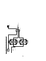
A test setup was constructed to identify the parameters of the prototype MR brake
(Figure 6.1). The setup consisted of a torque sensor (from Transducer Techniques, Inc.
[52]) attached to the brake chassis, a brush assembly to allow multiple rotations of the
shaft and a high precision potentiometer to measure position. Real time control was
implemented using a Quanser Q4 Series hardware-in-the-loop board connected to
SIMULINK via WinCon software [51].
Force sensor
MR Brake
Potentiometer
Brush assembly
Figure 6.1. Experimental setup for rotary MR brake.
44
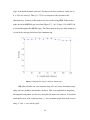
6.1.1 Braking Torque
In this experiment, the goal was to determine the braking torque as a function of
coil current. The current on the coil was increased by 0.1 A starting from zero to 1.5 A.
Then, the current was decreased using the same step size. The data from each step was
taken in 3 minute intervals to achieve consistency in readings. Figure 6.2 shows
torque/current curve for the full range of the braking torque. The minimum (off-state)
and maximum torque were found as 0.08 Nm and 10.9 Nm, respectively. This gives a
dynamic range of about 43 dB.
Figure 6.2. Braking torque of rotary MR brake versus current
6.1.2 Wall Collision
The experimental setup was converted into a 1-DOF haptic device by attaching a
lever arm to the MR Brake. The purpose of this experiment was to observe how well the
brake could simulate a collision with a virtual wall (surface). The control loop was
running at 1000 Hz with 1 A current for the brake during collision. The current was
45
turned on fully when collision occurred. The experiment was first conducted in two
modes: (1) without the torque sensor, and (2) with the torque, sensor to see the effect on
the haptic behavior. Algorithm for the wall collision experiment with the torque sensor is
as follows:
while simulation is running
if position is inside the wall and torque is towards the wall
activate brake in forward direction
else if readyToDemagnetize is true and brake is active
reset counter
set readyToDemagnetize to false
activate brake in reverse direction
else
deactivate brake
end if
if counter > demagnetizationDutation
set readyToDemagnetize to true
deactivate brake
end if
end while
46
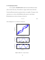
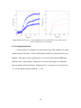
The results of virtual wall simulation without the torque sensor are presented in
Current (Amps)
Figure 6.3a and 6.3b.
1
0
-1
0
2
4
6
8
10
6
8
10
6
8
10
Time (s)
Torque (N/m)
5
0
-5
-10
0
2
4
Time (s)
Velocity (m/s)
2
0
-2
-4
0
2
4
Time (s)
(a)
Torque (N/m)
5
0
-5
-10
0
0.2
0.4
0.6
Position (rad)
0.8
1
(b)
Figure 6.3. Simulation of collision with a virtual wall located at position zero without using the torque
sensor. (a) Input current, torque and velocity. (b) Virtual wall at position 0. The lever arm is first
rotated away from position zero through approximately 0.95 radians. Then, it is rotated back towards
the virtual wall for collision simulation.
47
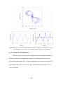
The results of virtual wall simulation with the torque sensor are presented in
Current (Amps)
Figure 6.4a and 6.4b.
1
0
-1
0
2
4
6
Time (s)
8
10
0
2
4
6
Time (s)
8
10
0
2
4
6
Time (s)
8
10
Torque (N/m)
5
0
Velocity (m/s)
-5
2
0
-2
Torque (N/m)
(a)
4
2
0
0
0.2
0.4
0.6
Position (rad)
0.8
1
(b)
Figure 6.4. Simulation of collision with a virtual wall located at position zero with the torque sensor. (a)
Input current, torque and velocity. (b) Virtual wall at position 0. The lever arm is first rotated away
from position zero through approximately 0.9 radians. Then, it is rotated back towards the virtual
wall for collision simulation.
48
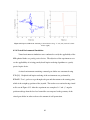
6.1.3 Damping Experiment
A servo amplifier (DR100EE20A8BDC-QD1 from Advanced Motion Controls
[55]) was added to the setup. This enabled us to supply variable current to the brake.
Closed loop PI current control was performed by the servo amplifier. The purpose of the
experiment was to see how well the MR brake could represent a virtual damper.
Relationship between velocity and torque was denoted as:
Τ = b ⋅ω
(6.1)
where damping ratio “b” was chosen as 1 Nm.s/rad.
6
Torque (N/m)
4
2
0
-2
-4
Velocity (rad/s)
Torque (N/m)
-6
-6
-4
-2
0
2
Velocity (rad/s)
4
6
5
0
-5
0
1
2
Time (s)
3
4
0
1
2
Time (s)
3
4
5
0
-5
Figure 6.5. MR brake as a damper in haptics.
49
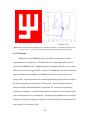
6.1.4 Coulomb Friction Experiment
We also explored the Coulomb friction characteristics of the MR brake. Karnopp
model was used to represent Coulomb friction due to its simplicity and ease of
implementation [56]. This model uses a velocity dead-band to define static friction range
instead of using absolute zero velocity which is very difficult to obtain with digital
systems due to discretization. The model can be represented as:
| ω |> ∆ω
Tdynamic ⋅ sgn(ω )
T friction =
max(Tstatic , Tapplied ) | ω |< ∆ω
(6.2)
where a 0.5 rad/s velocity-deadband ( ∆w ) was used and static friction torque
Velocity (rad/s)
Torque (N/m)
Torque (N/m)
Torque (N/m)
(Tstatic) was set at 5 Nm, dynamic friction torque (Tdynamic) was set at 3 Nm.
5
0
-5
-10
-5
0
Velocity (rad/s)
5
10
-10
-5
0
Velocity (rad/s)
5
10
5
0
-5
5
0
-5
0
1
2
Time (s)
3
4
0
1
2
Time (s)
3
4
10
0
-10
Figure 6.6. MR brake representing Coulomb friction.
50
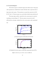
6.1.5 Transient Response
The transient response was obtained using the wall collision results. The purpose
of the experiment was to find the time constant of the brake and to explore the effect of
input current on the response. The experiment was repeated for current levels of 0.25,
0.5, 0.75 and 1A. Transient response was recorded after the initial contact with the wall.
The torque output resembles a typical first order system response in reaction to
step changes in current (Figure 6.7). The time constant was measured to be 60
milliseconds by overlaying a simulated first order system response on the experimental
data.
Torque (N.m)
8
6
4
2
0
0
0.2
0.4
Time (s)
0.6
0.8
(a) Transient response at 0.25A, 0.5A, 0.75A and 1A.
Torque (N.m)
8
6
4
2
0
0
0.2
0.4
Time (s)
0.6
0.8
(b) Simulated first-order response overlaid on the experimental data at 0.75A.
Figure 6.7. Transient response and time constant of the MR brake.
51
6.1.6 Discussion
Hysteresis behavior can be observed in the torque/current curves in figure 6.2.
This behavior is due to the magnetization of steel elements in the MR brake [57].
Magnetization in ferromagnetic elements does not relax back to zero even if the imposing
magnetic field is removed. Unfortunately, this behavior not only adversely affects the
controllability of the MR brake but also increases the off-state torque greatly. In our
experiments the residual magnetization kept the off-state torque at 1.05 Nm after
applying and removing 1.5A coil current. It caused unwanted off-state friction and
reduced the backdrivability of the brake. To overcome this problem the controller was
modified. At the instant the brake was turned off it was reactivated in the reverse
direction with a very short current impulse. An impulse with amplitude of 1A and 55 ms
duration (Current plot in Figure 6.3a and 6.4a) was found to be enough to collapse the
residual magnetic field reducing the off-state torque to 0.08 Nm from 1.05 Nm.
The effect of hysteresis is even more apparent in the damper experiment (Figure
6.5). This was mainly caused by the continuous nature of this experiment leaving no
time to apply current in the reverse direction in order to demagnetize the brake. As a
result, the system output two different torque outputs for a given velocity and also limited
the minimum amount of viscous torque that could be simulated with the system. Another
difficulty in this experiment was the time lag of the system having an adverse effect on
the simulation performance. Delays in discrete velocity calculations sometimes caused
incorrect torque outputs during acceleration and deceleration.
When the torque sensor was used, our experiments with the virtual wall
simulation produced a very crisp reaction force upon initial contact and very high rigidity
52
at the quasi-static contact with the wall (Figure 6.4). When the lever arm collided with
the virtual wall, the brake locked the position of the arm at zero radian. This created a
very rigid wall feeling. If the user tried to push the arm into the wall, the reaction torque
increased sharply (top vertical part of the curve in Figure 6.4b). When the lever was
pulled away from the wall, there was about 0.5 Nm torque acting in the reverse direction
as the separation occurred. Then, the brake turned off completely providing nearly zero
resistance. Most likely the time lag of the brake coupled with the delay in deactivating
the brake due to the demagnetization action caused the small initial torque in the reverse
direction. On the other hand, when the torque sensor was not used, the release action
from the wall had a “sticky” feeling (Figure 6.3b). This was due to the fact that the brake
was controlled only with position feedback. Once the wall penetration occurred, the
controller had no way of knowing the direction of the user input. As the user tried to pull
away from the wall, the release torque was almost as high as the maximum torque the
brake could apply (bottom vertical part of the curve in Figure 6.3b). This caused the
“sticky” wall feeling and also increased the observed velocities after the release since the
user had to pull the handle very hard to break away from the virtual wall.
It was found that the MR brake could simulate coulomb friction with good
accuracy. Although the mathematical model for such a simulation is rather simple, active
actuators (actuators that can add energy into the system) such as servo motors have great
difficulty in simulating discontinuous forces because of stability issues [56].
The transient response of the brake closely resembled first order system behavior
with a time constant of 60 ms. The experiment was repeated for different input currents
and it was found that input current had no effect on the time constant.
53
The 10.9 Nm maximum torque output obtained from the experiments was slightly
higher than the 10.83 Nm obtained from the calculations. This small deviation can be
attributed to mathematical simplifications, such as Bingham Plastic model, inherent
errors that were caused by finite element analysis of the magnetic field and neglecting
some physical effects such as Coulomb friction.
54
6.2 Spherical MR Brake Experiments
A series of experiments were conducted with two objectives in mind. First
objective was to identify the parameters of prototype spherical MR-brake and the second
objective was to test the applicability of the brake to a haptics environment.
6.2.1 Braking Torque
In this experiment, the goal was to determine the braking torque as a function of
coil current. The current on the coil was increased by 0.1 A starting from zero to 1.5 A.
Then, the current was decreased using the same step size. The data from each step was
taken in one minute intervals to achieve consistency in readings.
As shown in Figure 6.8, the minimum (off-state) and maximum torque were
found as 0.1 Nm and 3.7 Nm, respectively. This gives a dynamic range of about 31 dB.
Figure 6.8. Hysteretic braking torque of spherical MR brake versus current (Light gray: zero to 1.5 A,
dark gray: 1.5A to zero).
55
6.2.2 Wall Collision
A virtual wall was placed into the simulation environment. The purpose of this
experiment was to assess how well the brake could simulate collision with a virtual
surface (wall). A command force vector comes from the virtual environment and is
normal to the wall surface. An input vector comes from the force applied to the joystick
handle by the user indicating the intended motion. The control algorithm compares these
vectors. If the dot product of the vectors is negative, this means the user is trying to
penetrate the wall further and hence the brake is engaged. Furthermore, the controller
implements a demagnetization algorithm to flush out the residual magnetic field in the
brake after the joystick was pulled away from the wall.
56
The algorithm for the wall collision experiment is as follows:
while simulation is running do
if dotProduct(commandForce, userForce) < 0
(Condition for engaging the brake)
activate brake in forward direction
else if readyToDemagnetize is true and brake is active
(Condition for demagnetization)
reset counter
set readyToDemagnetize to false
activate brake in reverse direction
else
(Condition for deactivating the brake)
deactivate brake
end if
if counter > demagnetizationDutation
(Setting the demagnetization duration)
set readyToDemagnetize to true
deactivate brake
end if
end while loop
Where “commandForce” is the force vector from the virtual environment and
“userForce” is the input force obtained through the force sensor; “readyToDemagnetize”
and “demagnetizationDutation” are variables used for controlling the demagnetization.
57
To conduct the wall collision experiment the brake was driven at 1.5A current
using the Quanser board.
Figure 6.9. Simulation of collision with a virtual wall at position ߠ௫ = 0. The joystick handle is first
pulled away from position zero through approximately 0.45 radians. Then, it is pushed back towards
the virtual wall for the collision simulation.
6.2.3 Transient Response
The transient response was obtained using the wall collision simulation. The
purpose of the experiment was to find the time constant of the brake and to explore the
effect of input current on the response. The experiment was repeated for current levels of
0.5, 1 and 1.5A. Transient response was recorded after the initial contact with the wall.
First order system behavior was observed, time constant was found as 170ms for all 3
current levels (Figure 6.10).
58
Figure 6.10. Transient response of spherical MR-brake (left). Simulated first order system responses
used to estimate the time constant (right).
6.2.4 Damping Simulation
A linear analog servo amplifier was added to the setup. This enabled us to supply
variable current to the brake. Closed loop PI current control was performed by the servo
amplifier. The purpose of the experiment was to see how well the spherical MR-brake
could represent a virtual damper. Equation 6.1 was used for denoting the relationship
between angular velocity and torque. Damping ratio “b” was chosen as 1 N.m.s/rad and
“ ”ݓwas the angular velocity around the “y” axis.
59
Figure 6.11. Viscosity simulation with the MR spherical brake as a damper (top). Breakdown of torque
(left) and angular velocity around “y” axis (right) components of the viscosity simulation.
6.2.5 Coulomb Friction Simulation
The same setup as in the viscosity experiment was used to explore the ability of
the brake to simulate Coulomb friction (Figure 6.12). Karnopp model was used to
represent Coulomb friction [56]. Velocity-deadband (∆ )ݓwas selected as 0.3 rad/s and
static friction torque (Tstatic) was set at 2.5 Nm. The dynamic friction torque (Tdynamic)
was set at 0.5 Nm.
60
Figure 6.12. Spherical MR-brake simulating Coulomb friction along “x” axis (left), desired Coulomb
friction (right).
6.2.6 Virtual Environment Simulation
Virtual environment simulations were conducted to verify the applicabilty of the
MR spherical brake as a purely passive device. The objective of the experiment was to
see the applicability of existing penalty based haptic rendering algorithms to a purely
passive haptic device.
A virtual environment containing a manual gear shifter was constructed using
X3D [58]. Graphical and haptic rendering of the environment was performed by
H3DAPI. User’s goal was to go through each gear and then return to the starting point,
which is the straight up position of the joystick. The tracker was restricted using virtual
walls seen in Figure 6.13. After the experiment was completed “x” and “y” angular
position readings from the low level controller was compared to the geometry of the
virtual gear shifter in order to observe the amount of wall penetration.
61
Figure 6.13. Virtual environment simulation for a manual gear shifter in an automobile (left). Recorded
joystick positions as a user tries to shift gears with haptic feedback from the joystick (right).
6.2.7 Discussion
Similar to the rotary MR brake, hysteresis behavior can be observed in the
torque/current curves (Figure 6.8). This behavior is due to the magnetization of steel
elements in the MR brake [57]. Magnetization in ferromagnetic elements does not relax
back to zero even if the magnetic field is removed. Unfortunately, this behavior not only
adversely affects the controllability of the MR brake but also increases the off-state
torque greatly. In our experiments the residual magnetization kept the off-state torque at
0.3 Nm after applying and removing 1.5A coil current. It caused unwanted off-state
friction and reduced the backdrivability of the brake. To overcome this problem the
controller was modified. At the instant the brake was turned off it was reactivated in the
reverse direction with a very short impulse. An impulse with amplitude of 1A and 55 ms
duration was found to be enough to collapse the residual magnetic field reducing the offstate torque to 0.1 Nm from 0.3 Nm.
62
Spherical MR brake was also able to simulate Coulomb friction with good
accuracy (Figure 6.12).
Maximum torque that can be applied on “x” and “y” axes was found
experimentally to be 3.7 Nm. FEM simulations predicted it to be 3.28 Nm. The 11.4%
difference is probably due to friction forces from the O-Ring seal combined with the
increased contact force between the ball and socket due to the present magnetic field.
First order system response was observed during the activation of the brake.
Time constant was found to be approximately 170ms regardless of the applied current.
At higher torques there was visible deflection on the joystick handle and it might have
adversely affected the transient response of the system.
Virtual environment simulation using the manual gear shifter revealed that the
joystick could create very realistic contact with the virtual surfaces. Our experiments
with the virtual wall simulation produced a very crisp reaction force upon initial contact
and very high rigidity at the quasi-static contact with the wall (vertical part of the curve in
Figure 6.9). However several artifacts on force feedback were observed due to the purely
passive nature of the device. The most significant was the high friction on the virtual
surfaces. Since passive devices can only create forces against the user’s direction of
motion, it is impossible to create frictionless wall surfaces. After the initial contact with
the wall, if the user wanted to slide on the wall surface, the brake had to be kept engaged
in order to prevent further penetration into the wall. This resulted in friction forces that
were as high as contact forces on virtual surfaces. Another artifact was the problem
caused by noise in the optical positioning system. When the joystick was kept very close
to the wall surface, the noise in the positioning system caused the tracker to penetrate the
63
wall surface even though no motion was present in that direction. Since demagnetization
was performed after each wall collision to increase the backdrivability of the device, it
resulted in slight magnetization in the opposite direction or friction due to the combined
effect of the demagnetization pulses. This problem can be avoided in the future by using
a different positioning system or using optical sensors with better noise characteristics.
64
6.3 Passive Haptic Interface Experiments
Two set of experiments were conducted with the developed dental implant aid
system. The first set involved characterization of the device in displaying rigid virtual
objects. The second set involved analysis of the overall accuracy of manipulation tasks
with the system as a group of users tried to drill holes in polyurethane foam simulating
the dental implant surgery.
6.3.1 Virtual Wall Collision
(a)
(b)
(c)
Figure 6.14. Collision of the tip with a virtual wall.
65
Wall collision experiments were conducted for a very stiff wall (݇ = 10 ܰ/݉݉).
A wall surface was created at 0.8 m using H3DAPI (Figure 6.14). Starting at 0.9 m the
hand-piece of the haptic arm was moved towards the wall until the tip made contact with
the wall. As the tip was pressed into the wall, the force felt in the user’s hand increased
to about 15 N. Then, the contact with the wall was kept for about 1 second and the handpiece was moved away from the wall back to the 0.9 m position.
The results show very rigid wall collision with clean release. However, as it can
be seen on Figure (6.14) there is significant off-state friction. This off-state friction is
mainly due to magnetization of steel elements inside the MR brake leaving a residual
magnetic field over the MR fluid, hence higher off-state torques even when the current to
the brake is turned off. Previously, we were able to collapse the residual magnetic field
by giving a reverse current pulse to the brake (Figure 6.4a). This reduced the off-state
torque from about 10% of the full torque range down to about 1%. This result was
encouraging but had limitations. It is nearly impossible to implement this approach in
applications where the MR-brake needs to apply variable torque as an actuator. In the
duration of the reverse pulse the brakes cannot be engaged. Tasks such as wall following
become very difficult since they require continuous brake control.
6.3.2 Virtual Wall Following
Wall following experiments were conducted to analyze the haptic arm’s ability to
simulate moving over a virtual wall surface. A virtual environment containing flat walls
were created using H3DAPI. The experiment consisted of dragging the tracker (virtual
arm tip) along the virtual wall surface.
66
Because of the force approximation in the control system, the haptic arm showed
varying wall following performance at different locations in its work volume. If the
mechanism was at a configuration such that the force vector created by the haptic device
could be rendered normal to the virtual wall surface then frictionless walls could be
rendered. However if the mechanism was in a configuration such that the force vector
contained tangential and normal components, then the reality of the wall following task
suffered. This was because of the passive MR brakes on the haptic arm, which limited
the direction of the force vector to certain angles according to the wall and the user force
vector directions.
In order to demonstrate this phenomenon the experiment was conducted at two
different zones inside the work volume. In one zone the system could display smooth
walls while in the other it could not.
6.3.2.1 Smooth Wall Display
A vertical virtual wall with (݇ = 0.5 ܰ/݉݉) was created on y = -0.8 m plane.
The “y” and “z” coordinates of the wall following task can be seen in Figure 6.15.
67
(a)
(b)
Figure 6.15. Smooth wall display.
6.3.2.2 Unsmooth Wall Display
A horizontal virtual wall with (݇ = 0.5 ܰ/݉݉) was created on z = 0 plane. The
“y” and “z” coordinates of the wall following task can be seen in Figure 6.16.
(a)
(b)
Figure 6.16. Unsmooth wall display.
68
Figures 6.15b and 6.16b reveal a significant difference in the rendered wall
quality. Figure 6.15b shows a smooth wall surface -albeit slightly curved-, whereas
Figure 6.16b shows a “jagged” wall. Both of these shapes are the result of the force
approximation algorithm. For the smooth wall display, the controller renders the wall
almost frictionless by locking joint 2 at the same time releasing joints 1 & 3, resulting in
the arc seen in Figure 6.15a. For the unsmooth wall display the controller does almost
the same thing initially by locking joint 2 and releasing joints 1 & 3. However, the
resulting arc is not parallel to the wall surface (Figure 6.16a). When the user drags the
hand-piece along the wall surface, he/she is constrained on this arc, creating a much
desired –although artificial- pullback action, at the same time giving the wall its “jagged”
feeling.
6.3.3 Drilling with Haptic Feedback
6.3.3.1 Objective
The goal of this experiment was to analyze the overall accuracy of manipulation
tasks with the system. The experiment involved drilling holes in polyurethane foam
simulating the dental implant surgery. The hypothesis was that the passive haptic device
would result in positioning accuracies similar to or better than the accuracies of other
dental surgery systems.
6.3.3.2 Procedure
Twenty one users (18 male and 3 female) performed the usability experiment.
Each user first went through a training session where the experiment setup was
introduced. The users then performed a trial run where they placed holes at 3 different
69
locations. No data was collected during the trial run and the hole locations were different
than the actual experiment.
Figure 6.17. Usability experiments
Following the training, the real placement task was performed 3 times by each
user. The hole placement order was randomized to prevent any task learning. There was
no time constraint on the experiment. In between trials, the user was allowed to rest
his/her arm for one minute. Users were instructed to drill three holes with the assistance
of the haptic feedback coming from the device (Figure 6.17). Hole locations were guided
by virtual constraints that resembled angle brackets in the virtual environment (Figure
6.18). The corner of each virtual bracket was aligned with the axis of a hole. The users
moved the hand-piece to position the tracker (virtual tip) near a guide. After that, they
pressed the tracker against both walls of the virtual bracket and felt the haptic feedback in
their hand to locate the x and y positions of the hole. To successfully guide the drill bit
along the axis, the users had to keep the tracker in contact with the bracket through haptic
feedback in their hand as they moved the bit down towards the foam. The z-depth of the
holes was fixed by a horizontal virtual wall inside the foam. As the user continued to
70
penetrate the foam, the arm locked up when the required depth was reached by the drill
bit. A total of 3 holes had to be drilled for each placement task. The holes were located
50mm apart in an “L” shaped arrangement and the depth was limited at 4 mm.
Figure 6.18. Virtual environment for haptic hole placement
6.3.3.3 Results
After the experiment the hole locations were carefully measured using a caliper.
In each measurement deviation from actual dimensions ( = ݕ = ݔ50݉݉ & = ݖ4݉݉)
was calculated as the positioning error. The average error for each dimension and the
standard deviation are given in Table 6.1.
Table 6.1: Results of haptic drilling experiment
Error
Standard deviation
x-axis
2.88mm
2.51mm
y-axis
1.90mm
1.46mm
z-axis
1.16mm
0.94mm
71
6.3.3.4 Discussion
An image-guided implantology system had an average error of 1.23 ± 0.28 mm
and maximum error of 1.87 ± 0.47 mm [19]. Robot assistant systems report deviations of
1 - 2 mm [23, 24]. Our passive haptic system had errors below 2 mm for “y” and “z” axis
and a little below 3 mm for the “x” axis. These results are on the same order of
magnitude as the optical tracking system and other dental robots, hence passive haptic
devices have potential to be a viable alternative to active (servo controlled) haptic
devices.
Deflection was the primary cause for the errors. Although the haptic arm was
built with deflection in mind by using materials such as steel, aluminum and carbon fiber
as opposed to polymer based materials common in today’s haptic devices, main cause of
the errors was the deflection in the system. This became especially problematic in the xaxis direction as forces in this direction resulted in torsion of the mechanism out of the
plane of the parallel links in the mechanism. This resulted in the highest average error
among all three axes (2.88mm).
Another cause for the deviation –although not as significant as the first cause- was
the lack of pull back action on the virtual walls. This is possible with haptic devices with
active actuators such as motors. The passive actuators can only create resistance forces.
If the user penetrated into the wall by pressing too hard, the system had no way of
compensating for the error since it could not pull back the tip.
A final cause was the resistance force created by the foam due to the penetration
of the drill bit. Some users mistook the haptic feedback for limiting the “z” depth as the
resistance force of the foam and continued to press down looking for the haptic feedback
72
to stop. When the manipulator and the haptic master are the same device, haptic
feedback forces and reaction forces from the environment are bound to overlap. This
kind of effect would be more significant when drilling a more rigid object such as bone.
A viable solution would be to measure the reaction forces coming from the environment
and make necessary compensations in the haptic force feedback accordingly.
73
CHAPTER 7
CONCLUSIONS AND FUTURE RECOMMENDATIONS
A novel haptic interface with MR brakes for dental implant surgery has been
built. As part of this research, rotary MR brakes with high torque output have been
developed using the serpentine flux path technique. The design activates more surface
area of the MR fluid in a given volume by weaving the magnetic flux through the MR
fluid multiple times. Table 7.1 compares the design specifications of the rotary brake to a
commercially available MR brake.
Table 7.1: Design Specifications of the Rotary MR-Brake
Diameter (mm)
Length (mm)
Max. torque (Nm)
Max. off-state (Nm)
Max. current (A)
Time constant (ms)
Designed
MR-Brake
(RD-2087-01
by LORD Corp.)
63.5
89.7*
10.9
< 0.1
1.5
60
96.6
43.7
4.0
< 0.4
1.0
-
*Includes ferro-fluidic seal end caps (27.0 mm).
The prototype MR brake is about 2.7 times more powerful than the commercially
available RD-2087-01 rotary brake by Lord Corporation and about 33% smaller in
diameter. Furthermore, with 10.9 Nm torque output, it is more powerful than the closest
brake in the literature with 6.9 Nm torque [30] but only approximately half the diameter
and requires 62.5% less current.
Another contribution of the research was a ferro-fluidic seal which reduced the
74
friction that would normally occur due to using conventional O-rings. The off-state
friction was further reduced down to a negligible 0.08 Nm by applying a current pulse in
the reverse direction. This improved the backdrivability of the brake which is much
desired in haptics applications.
Current prototype is capable of rendering only 3-DOF (x-y-z position). In future
studies, additional MR brakes can be added to the wrist joint to control the orientation,
effectively building a 6-DOF haptic display. Potential solutions already exists where
MR-brakes as small as a U.S. quarter [40] were previously designed. Another solution,
which was explored in this research, is a spherical MR brake [25] that is capable of
locking all 3-DOF at once. To the best of our knowledge, this design is the first ever
multi-DOF spherical brake using MR fluid.
The prototype spherical MR brake has a diameter of 76.2 mm and can apply up to
3.7 Nm braking torque. Since the torque is proportional to the cube of the radius of the
steel ball, the brake can scale up very well. Using this design it is possible to make much
more powerful brakes without increasing the overall dimension of the brake significantly.
An optical position measurement system that eliminated the gimbal mechanisms
that are typically used in spherical joints for position measurement was also developed as
part of this research. However, the optical sensors turned out to be susceptible to noise
leading to inaccuracies in the position measurements. Another method is necessary to
measure the position of the steel ball in the brake.
Design options for the wrist joint using small rotary brakes or the spherical brake
can be explored in a future study.
75
Experiments to identify the characteristics of the haptic interface for dental
surgery have been conducted. Initial experiments show that passive haptic devices can be
viable alternatives to active haptic devices.
During the haptic drilling experiments deflection caused positioning errors despite
the rigid construction of the haptic arm. This is a challenging issue since the arm needs
to be lightweight and the application requires very strict positioning accuracy. In the
future we plan to explore options for closed loop position control using optical/magnetic
trackers and/or a mathematical model of the deflection in order to compensate for the
positioning error.
Passive haptic devices have advantages over active devices in terms of stability,
rigid wall collision and inherent safety. They suffer from lack of pull back action on the
virtual walls, unsmooth behavior at the wall surfaces and inability to compensate for
positioning errors. All of these shortcomings can be overcome by designing devices that
use hybrid passive-active actuators [26, 27, 56].
76
BIBLIOGRAPHY
[1]
Fortin, T., Isidori, M., Blanchet, E., Perriat, M., Bouchet, H. and Coudert, J. L. “An
image-guided system-Drilled surgical template and trephine guide pin to make
treatment of completely edentulous patients easier: A clinical report on immediate
loading.” Clinical Implant Dentistry and Related Research. 6(2). Pages: 11-119.
2004
[2]
Bartling, R., Freeman, K. & Kraut, R.A. “The incidence of altered sensation of the
mental nerve after mandibular implant placement.” Journal of Oral and
Maxillofacial Surgery 57: 1408–1412. 1999
[3]
Ellies, L.G. “Altered sensation following mandibular implant surgery: a
retrospective study.” Journal of Prosthetic Dentistry 68: 664–671. 1992
[4]
Serhal, C. B., Steenberghe, D., Quirynen, M. and Jacobs, R. “Localisation of the
mandibular canal using conventional spiral tomography: a human cadaver study.”
In Clinical Oral Implants Research. 12(3). Pages 230-236. 2001
[5]
Berberi, A., Le Breton, G., Mani, J., Woimant, H. & Nasseh, I. “Lingual paresthesia
following surgical placement of implants: report of a case.” International Journal of
Oral and Maxillofacial Implants 8: 580–582. 1993
[6]
Berglundh, T., Persson L. and Klinge B. “A systematic review of the incidence of
biological and technical complications in implant dentistry reported in prospective
longitudinal studies of at least 5 years.” Journal Of Clinical Periodontology. 29(3).
Pages: 197-212. 2002
[7]
Gray ‘s Anatomy. 20th US Edition. 1918
[8]
Brief, J., Edinger, D, Hassfeld, S, Eggers, G. “Accuracy of image-guided
implantology.” Clinical Oral Implants Research, Volume 16, Number 4, August
2005 , pp. 495-501(7)
[9]
Buser, D., Martin, W., Belser, U. C. “Optimizing esthetics for implant restorations
in the anterior maxilla: Anatomic and surgical considerations.” Int J Oral
Maxillofac Implants. 19(7). Pages: 43–61. 2004
[10] Lal, K., White, G. S., Moreaand, D. N., Wright, R. F. “Use of stereolithographic
templates for surgical and prosthodontic implant planning and placement.” Part I.
The Concept. Journal of Prosthodontics. 15(1). Pages 51-58. 2006
[11] SurgiGuide, Materialize Medical. Available: [Online] http://www.materialise.com
Accessed: October, 2009
[12] CompuSurge Template, Implant Logic Systems. Available: [Online]
http://www.ipr.ira.uka.de/compusurge/ Accessed: October, 2009
[13] Simplant, Materialize Medical. Available: [Online] http://www.materialise.com
Accessed: October, 2009
77
[14] Klein, M., Abrams, M. “Computer-guided surgery utilizing a computer-milled
surgical template.” Pract Proced Aesthet Dent. 2001 Mar;13(2):165-9
[15] Sarment, D. P., Sukovic, P., Clinthorne., N. “Accuracy of implant placement with a
stereolithographic surgical guide.” The International Journal of Oral &
Maxillofacial Implants. 18(4). 2003
[16] Ewers, R., Truppe, M., Reichwein, A., Wagner A. “Computer-aided navigation in
dental implantology: 7 years of clinical experience.” Journal of Oral and
Maxillofacial Surgery, Volume 62, Issue 3, Pages 329-334
[17] Robodent, Robodent GmbH. Available: [Online] http://www.robodent.com/
Accessed: October, 2009
[18] IGI Denx, Image Navigation Ltd. Available: [Online] http://www.denx.com/
Accessed: October, 2009
[19] Birkfellner, W., Solar, P., Gahleitner, A., Huber, K., Kainberger, F., Kettenbach, J.,
Homolka, P., Diemling, M., Watzek, G., Bergmann, H.. “In-vitro assessment of a
registration protocol for image guided implant dentistry.” Clin Oral Implants
Res.;12(1):69-78. 2001
[20] Lueth, T.C.; Hein, A.; Albrecht, J.; Demirtas, M.; Zachow, S.; Heissler, E.; Klein,
M.; Menneking, H.; Hommel, G.; Bier, J., "A surgical robot system for
maxillofacial surgery," Industrial Electronics Society, 1998. IECON '98.
Proceedings of the 24th Annual Conference of the IEEE , vol.4, no., pp.2470-2475
vol.4, 31 Aug-4 Sep 1998
[21] Kusumoto, N., Sohmura, T., Yamada, S., Wakabayashi, K., Nakamura, T., Yatani,
H. “Application of virtual reality force feedback haptic device for oral implant
surgery.” Clinical Oral Implants Research, 17(6), Pages 708-713, 2006
[22] PHANToM, Sensable Technologies, Inc. Available: [Online] www.sensable.com
Accessed: October, 2009
[23] Brief, J, Hassfeld, S, Redlich, T, et al. “Robot-assisted insertion of dental
implants—a clinical evaluation.” Lemke HU, Vannier MW, Inamura K, Farman A,
eds. Computer assisted radiology and surgery. Proceedings of the 14th International
Congress and Exhibition, 28 June–1 July 2000, San Francisco, CA. Amsterdam:
Elsevier, 2000: 932–937.
[24] Boesecke, R., Brief, J., Raczkowsky, J., Schorr, O., Daueber, S., Krempien, R.,
Treiber, M., Wetter, T., and Haßfeld, S. 2001. “Robot sssistant for dental
implantology.” In Proceedings of the 4th international Conference on Medical
Image Computing and Computer-Assisted intervention (October 14 - 17, 2001). W.
J. Niessen and M. A. Viergever, Eds. Lecture Notes In Computer Science, vol.
2208. Springer-Verlag, London, 1302-1303.
[25] Senkal, D. and Gurocak, H.B. 2009. “Spherical brake with MR fluid as multi degree
of freedom actuator for haptics”, Journal of Intelligent Material Systems and
Structures (In press).
78
[26] An, J. and Kwon, D.S.. “Five-bar linkage haptic device with DC motors and MR
brakes.” In Journal of Intelligent Materials Systems and Structures, 00:1-12, 2008.
[27] An, J. and Kwon, D.S. “Haptic experimentation on a hybrid active/passive force
feedback device.” In Proceedings of the IEEE Int. Conf. on Robotics and
Automation (Washington DC, May 2002).
[28] Nam, Y.J. and Park, M.K. “A hybrid haptic device for wide-ranged force reflection
and improved transparency.” In Proceedings of the Int. Conf. on Control,
Automation and Systems (Seoul, Korea, October 17-20, 2007).
[29] Reed, M. and Book, W. “Modeling and control of an improved dissipative passive
haptic display.” In Proceedings of the Int. Conf. on Robotics and Automation (New
Orleans, LA, April 2004).
[30] Carlson, J.D., Leroy, D.F., Holzheimer J.C., Prindle, D.R. and Marjoram R.H.
“Controllable Brake.” US Patent No.: 5,842,547 (December, 1998)
[31] Kavlicoglu, B., Gordaninejad, F., Evrensel, C., Cobanoglu, N., Liu, Y. and Fuchs,
A. “A high-torque magneto-rheological fluid clutch.” In Gregory S. Agnes editor,
Smart Structures and Materials 2002: Damping and Isolation, Proceedings of SPIE
(vol. 4867, 2002).
[32] Demersseman, R., Hafez M., Lemaire-Semail, B. and Clenet, S.
“Magnetorheological brake for haptic rendering.” In M. Ferre editor, Proceedings
of the EuroHaptics 2008 (Spain, 2008).
[33] Li, W.H. and Du., H. “Design and experimental evaluation of magnetorheological
brake.” In Int. Journal of Manufacturing Technology, vol. 21, pages 508-515, 2003.
[34] Nam, Y.J, Moon Y.J. and Park. M.K. “Performance improvement of a rotary MR
fluid actuator based on electromagnetic design.” In Journal of Intelligent Materials
Systems and Structures, vol. 19, pages 695-705, June 2008.
[35] Li, W.H., Liu, B., Kosasih, P.B. and Zhang, X.Z. 2007. “A 2-DOF MR actuator
joystick for virtual reality applications,” Sensors and Actuators A: Physical,
137(2):308-320.
[36] Yamaguchi, Y., Furusho, J., Kimura S. and Koyanagi K. 2005. “Development of
high-performance MR actuator and its application to 2-D force display,”
International Journal of Modern Physics B, 19,(7-9):1485-1491.
[37] Han, Y.M., Kang, P.S., Sung, K.G. and Choi, S.B. 2007. “Force feedback control of
a medical haptic master using an electrorheological fluid,” Journal of Intelligent
Material Systems and Structures, 18(12):1149-1154.
[38] Bose, H. and Berkemeier, H.J. 1999. “Haptic device working with an
electrorheological fluid,” Journal of Intelligent Material Systems and Structures,
10(9):714-717.
79
[39] Senkal, D. and Gurocak, H.B. 2009. "Compact MR-brake with serpentine flux path
for haptics applications," World Haptics 2009 - Third Joint EuroHaptics conference
and Symposium on Haptic Interfaces for Virtual Environment and Teleoperator
Systems, Salt Lake City, Utah, 91-96
[40] Blake, J. and Gurocak, H.B. 2009. “Haptic glove with MR brakes for virtual
reality,” IEEE/ASME Transactions on Mechatronics (In press).
[41] H3DAPI, Sensegraphics AB. Available: [Online] http://www.sensegraphics.com/
Accessed: October, 2009
[42] Ruspini, D. C., Kolarov, K. and Khatib, O. 1997. “The haptic display of complex
graphical environments,” Proceedings of the 24th Annual Conference on Computer
Graphics and interactive Techniques, ACM Press/Addison-Wesley Publishing Co.,
New York, NY, 345-352
[43] Cho, C., Kim, M. Song, J.B., “Direct control of a passive haptic device based on
passive force manipulability ellipsoid analysis”, International Journal of Control,
Automation and Systems. 2(2). Pages 238-246. 2004
[44] Cho, C., Song, J.B., Kim, M, Hwang, C.S., "Energy-based control of a passive
haptic device," Robotics and Automation, 2004. Proceedings. ICRA '04. 2004 IEEE
International Conference on , vol.1, no., pp. 292-297 Vol.1, 26 April-1 May 2004
[45] Infolytica Corp. [Online]. Available: http://www.infolytica.com/ Accessed:
October, 2009
[46] Lord Corp. [Online]. Available: http://www.lord.com/ Accessed: October, 2009
[47] Tsumaki, Y., Naruse, H., Nenchev, D.N. and Uchiyama, M. 1998. "Design of a
compact 6-DOF haptic interface," Proceedings of the 1998 IEEE International
Conference on Robotics & Automation, Leuven, Belgium, vol.3, 2580-2585
[48] Rosenberg, L. B. and Adelstein, B. D. 1993 “Perceptual decomposition of virtual
haptic surfaces,” Proceedings, IEEE Symposium on Research Frontiers in Virtual
Reality, IEEE Computer Society Press, Los Alamitos CA, 46-53
[49] MathWorks Inc. [Online]. Available: http://www.mathworks.com/
[50] Bourns, Inc. Available: [Online] http://www.bourns.com/ Accessed: October, 2009
[51] Quanser. Available: [Online] http://www.quanser.com/ Accessed: October, 2009
[52] ATI Industrial Automation, Inc.. Available: [Online] http://www.ati-ia.com/
Accessed: October, 2009
[53] National Instruments. Available: [Online] http://www.ni.com/ Accessed: October,
2009
[54] Sakaguchi, M.; Furusho, J.; Takesue, N., "Passive force display using ER brakes
and its control experiments," Virtual Reality, 2001. Proceedings. IEEE , vol., no.,
pp.7-12, 17-17 March, 2001
80
[55] Advanced Motion Controls. [Online]. Available: http://www.a-m-c.com Accessed:
October, 2009
[56] An J. and Kwon D.S., “Stability and Performance of Haptic Interfaces with
Active/Passive Actuators – Theory and Experiments.” In Int. Journal of Robotics
Research, vol. 25, no.11, pages 1121-1136, November, 2006
[57] Liu B.,Li WH., Kosasih P. B. and Zhang X. Z.. “Development of an MR-brakebased haptic device.” In Smart Materials and Structures. vol. 15, no 6, pages 19601966, 2006.
[58] Web3D Consortium. [Online]. Available: http://www.web3d.org/ Accessed:
October, 2009
81
APPENDIX A: ASSEMBLY DRAWINGS
82
83
84
85
86
87
88
APPENDIX B: SOFTWARE
89
90
Posi tionInput
v elocity X
v elocity Y
wallStateout
H3DAPIcommandOut
angleOut
Viscosity ControllerOutput
CoulomVontrollerOutput
demagnetizationControl ler
demagnetizationControllerOutput
CoulombFricti onController
v elocity Y
v elocity X
ViscosityController
v elocity Y
v elocity X
HighLevelController
positionY in
positionY
positionZ
positionXin
f orceXin
f orceY in
positionX
ForceSensor
ForceY
ForceX
Si mul ationNo
4
demagnetizedCommandOutput
demagnetizationControl ler1
commandInput
angleInput
B.1.1 Spherical Brake Simulink Diagram
B.1 SOFTWARE FOR SPHERICAL MR BRAKE
Simulation Selecti on
commandSignal
rawCommandSignal
91
ATI F/T Sensor
F/T output
ForceSensorNo
2
ForceSensorSwitch
Jacobian
y Output
ATIinput
xOutput
ForceY
ForceX
2
f orceX
SecondaryForceSensor
1
f orceY
B.1.1.1 Force Sensor Sub-system
forceXYvector
92
Windows Keyboard1
Is the
C
key pressed?
Analog Input
National Instruments
NIE ADC
Windows Keyboard
Is the
C
key pressed?
Gain1
-17
Gain
-15
B.1.1.2 SecondaryForceSensor Sub-system
Calibration
input
Calibration1
Calibration2
keyState
input
Calibration1
keyState
out
out
2
1
forceX
forceY
ForceX
ForceY
ForceVector
93
Analog Input FT
National Instruments
NIE ADC
Windows Keyboard
Is the
C
key pressed?
20
20
s+20
s+20
20
20
20
s+20
20
s+20
20
20
s+20
Di scretized
T ransfer Function12
Discretized
Transfer Function11
s+20
20
s+20
Di scretized
T ransfer Function5
Discretized
Transfer Function6
Discretized
Transfer Function10
Discretized
Transfer Function9
s+20
20
s+20
Discretized
Transfer Function4
Discretized
Transfer Function2
Discretized
Transfer Functi on8
Discreti zed
Transfer Functi on7
s+20
20
s+20
Discretized
Transfer Function3
Discreti zed
Transfer Functi on1
s+20
20
B.1.1.3 ATI F/T Sensor Sub-system
i nput
BiasFT
CalibrationFT 2 out
keyState
CalibrationMatrix
K*u
ScalingFactor
-K-
1
F/T output
94
AT Iinput
1
Jacobian
K*u
FTsensorRaw
B.1.1.4 Jacobian Subsystem
2
xOutput
1
yOutput
FTsensorJacobian
XGain
-1
YGain
-1
95
Integer Delay1
-50
Z
Integer Delay
-25
Z
Constant2
-1.1303
Analog Input1
Quanser
Q4 ADC
Gain6
1
Gain4
4
3
Math
Function
uv
Subtract
Gain7
Gain2
5.078
Gain1
20
d
positionX
s+25
25
velocityX
5
velocityX1
Worlds Most Primitive Haptic Device
Controller
-25
Z
2
Gain8
1
Gain5
4
3
positionZ
3
positionY
positionY1
Integer Delay3
-50
Z
1
positionX
positionX1
Integer Delay2
positionZ
TriangulationTransform positionY
Discretized
Transfer Function3
Sensor Distance
B.1.1.5 PositionInput Sub-System
25
Subtract1
Gain9
Discretized
Transfer Function1
s+25
25
Discretized
Transfer Function
s+25
Gain3
20
Discretized
Transfer Function2
s+25
25
velocityY
4
velocityY2
PositionVector
96
PowerupDel ay
YinYout
posi tionYi n
Xin Xout
3
posi tionXi n
4
Button1
0
writeTimeout
readTimeout
commandTorqueZ
commandTorqueY
commandTorqueX
commandForceZ
commandForceY
1
forceXin
2
forceYin
Pin5
commandForceX
H3DAPI
orientationRoll
orientationPitch
orientationY aw
v elocity Z
v elocity Y
v elocity X
positionZ
positionY
positionX
Pin4
90
B.1.1.6 HighLevelController Sub-system
outAngle
outCommand
outForceAbs
outWallState
Desi redForce
WallCol lissionHapti cControl ler
transitionAngle
wallAngl e
commandForceY
WallCol lissionHapti cControl ler
commandForceX
forceX
forceY
1
ForceAbs
wallStateout
3
angleOut
2
commandSignalRaw
H3DAPIcommandOut
97
Button1
orientationRoll
10
orientationPitch
9
orientationYaw
8
velocityZ
7
velocityY
6
velocityX
5
positionZ
4
positionY
3
positionX
2
1
B.1.1.7 H3DAPI Sub-system
Write Shared Memory
Quanser WRMEM
No handshaking
Read Shared Memory
Quanser RDMEM
No handshaking
writeTimeout
8
readTimeout
7
commandTorqueZ
6
commandTorqueY
5
commandTorqueX
4
commandForceZ
3
commandForceY
2
commandForceX
1
98
angleInput
1
duration
55
commandInput
2
inputAngle
demagnetDuration
Input
DemagnetizationController
DemagnetizationController1
B.1.1.8 demagnetizationController1 Sub-system
Pin3
0
Pin1
-1
selector
DemagnetizationSwitch
1
demagnetizedCommandOutput
99
velocityY
velocityX
ViscosityController
ViscosityController
Pin7
0
outVelocity
coulombThreshold
0.3
velocityY
2
velocityX
1
threshold
velocityY
velocityX
CoulombController
1
outVelocity
viscosityGain
2/2.5
CoulomVontrollerOutput
CoulombController outCommand
B.1.1.10 CoulombFrictionController Sub-system
velocityY
2
velocityX
1
B.1.1.9 ViscosityController Sub-system
1
ViscosityControllerOutput
100
55
inputCurrent
rawCommandSignal
1
ServoAmpGain
2.1850
Voltage
1
Analog Output
Quanser
Q4 DAC
pin0
1
demagnetizationControllerOutput
commandSignalOutput
DemagnetizationController
demagnetDuration DemagnetizationController
Input
B.1.1.12 commandSignal Sub-system
InputCurrent
1
duration
Windows Keyboard
Is the
L
key pressed?
B.1.1.11 demagnetizationController Sub-system
B.1.2 Spherical Brake Simulink Code
Calibration Block
Discrete update:
if(keyState[0] == 1){
xD[0] = input[0];
}
Output:
out[0] = xD[0];
BiasFT Block
Discrete update:
int i;
if(keyState[0] == 1){
for(i=0; i<6; i++){
xD[i] = input[i];
}
}
Output:
int i;
for(i=0; i<6; i++){
out[i] = xD[i];
}
TriangulationTransform Block
Discrete update:::
double x1, y1, z1, x2, y2, z2, x3, y3, z3, A, B, C, D, betaPrime;
x1 = 1.0625 + 0.5 * d[0];
y1 = 0;
z1 = 0.866 * d[0];
x2 = 1.0625*(-0.5) + (-0.5)*0.5*d[1];
y2 = 1.0625*(0.866) + (0.866)*0.5*d[1];
z2 = 0.8660*d[1];
x3 = 1.0625*(-0.5) + (-0.5)*0.5*d[2];
y3 = 1.0625*(-0.866) + (-0.866)*0.5*d[2];
z3 = 0.8660*d[2];
A
B
C
D
=
=
=
=
y2*z3 + y1*z2 + z1*y3 - x1*y2 x1*z3 + x2*z1 + x3*z1 - z1*x3 x1*y2 + x2*y3 + y1*x3 - y1*x2 (x1*y2*z3 + x2*y3*z1 + y1*z2*x3
z2*y3 - z3*y1;
z2*x1 - z3*x2;
y2*x3 - y3*x1;
- z1*y2*x3* - z2*y3*x1 - z3*y1*x2);
xD[0] = asin(-B/sqrt(A*A+B*B+C*C));
xD[1] = asin(-A/sqrt(A*A+B*B+C*C));
xD[2] = C/sqrt(A*A+B*B+C*C);
Output:
positionX[0] = xD[0];
101
positionY[0] = xD[1];
positionZ[0] = xD[2];
wallCollisionHapticController Block
Discrete update:::
double forceAngle;
int wallState;
forceAngle =
acos((commandForceX[0]*forceX[0]+commandForceY[0]*forceY[0])/pow((force
X[0]*forceX[0]+forceY[0]*forceY[0]),0.5)/pow((commandForceX[0]*commandF
orceX[0]+commandForceY[0]*commandForceY[0]),0.5))/3.141592653589793*180
;
if(forceAngle>=360){forceAngle = 360;}
if(forceAngle<=-360){forceAngle = -360;}
xD[1] = forceAngle;
xD[2] = pow((forceX[0]*forceX[0]+forceY[0]*forceY[0]),0.5);
if(abs(forceAngle)>wallAngle[0]+transitionAngle[0]){
xD[0] = 1;
wallState = 1;
}
else if(abs(forceAngle)>wallAngle[0] &&
(wallAngle[0]+transitionAngle[0])>abs(forceAngle)){
xD[0] = (abs(forceAngle)-wallAngle[0])/transitionAngle[0]*2.5;
wallState = 2;
}
else{
xD[0] = 0;
wallState = 0;
}
Output:
outCommand[0] = xD[0];
outAngle[0] = xD[1];
outForceAbs[0] = xD[2];
demagnetizationController1 Block
Discrete update:
xD[6]++;
xD[2]++;
if(Input[0]>0) {
xD[0] = 1;
xD[4] = 1;
xD[5] = 0;
}
else {
if(Input[0]==0 && xD[4]==1 && abs(inputAngle[0])<=45) {
xD[5] = 1;
xD[4] = 0;
xD[3] = xD[2];
}
}
102
if(xD[5] == 1) {
xD[0] = -1;
}
if((xD[2]-xD[3])>demagnetDuration[0] && Input[0]==0) {
xD[5] = 0;
xD[0] = 0;
}
Output:
if(xD[0]==1) {
selector[0] = 1;
}
else if(xD[0]==-1){
selector[0] = 2;
}
else if(xD[0]==0){
selector[0] = 3;
}
velocityController
Discrete update:::
xD[0] = 1 * velocityX[0];
Output:
outVelocity[0] = xD[0];
CoulombController Block
Discrete update:
if(pow((velocityX[0]*velocityX[0]+velocityY[0]*velocityY[0]),0.5)<=thre
shold[0])
{
xD[0] = 1.5;
}
else
{
xD[0] = 0.1;
}
Output:
outCommand[0] = xD[0];
demagnetizationController Block
Discrete update:::
xD[2]++;
if(Input[0]>0) {
xD[0] = 1;
xD[1] = 0;
}
else {
103
if(xD[4] ==
xD[3] =
xD[4] =
xD[1] =
}
xD[0] = 0;
1 && xD[0]==1) {
xD[2];
0;
1;
}
if((xD[2]-xD[3])>demagnetDuration[0] || xD[0]==1) {
xD[1] = 0;
xD[4] = 1;
}
Output::
if(xD[0]>0)
pin0[0]
}
else{
pin0[0]
}
if(xD[1] ==
pin0[0]
}
{
= inputCurrent[0];
= 0;
1) {
= -1*inputCurrent[0];
104
105
t3offset
0
t2offset
2.8
t1offset
0
a3
t3offset
t2offset
t1offset
a3input
0.4857750
a2
a2input
volts
0.48
PotentiometerConditi oning
PotentiometerOutput
Simulati onNo
2
PotsVol tage2Angle
PotsVol tage2Angle
J
T04out
theta
Jout
T04out
theta
Jputput
userTorque
HighLevelControllerHookUp
userForce
commandForceH3DAPI-XYZ
Jinput
userForce
commandForce
ForceApproximation
commandTorqueInput ForceApproximationCommandOutput
Jinput
torque
LatchingController
LatchingControllerCommandOutput
commandTorqueH3DAPI
T04input
B.2.1 Haptic Surgical Aid System Simulink Diagram
B.2 SOFTWARE FOR HAPTIC SURGICAL AID SYSTEM
SimulationSel ector
CommandOutput
CommandSignalIn
106
Pots
Quanser
Q4 ADC
DampingSelector
1
PotFilter6
s+5
5
PotFilter5
s+5
5
PotFilter4
s+5
5
PotFilter3
s+200
200
PotFilter2
s+200
200
PotFilter1
s+200
200
B.2.1.1 PotentiometerConditioning Sub-system
PositionDamping
PotentiometerOutput
1
Pots Raw
107
2.1850
Windows Keyboard
Is the
L
key pressed?
Input Curent
1.5
Demagnet Duration
55
inputCurrent
MR Brakes
Quanser
Q4 DAC
LatchingController2
LatchingController2
commandOut
demagnetDuration
Input
Voltage Saturation
VoltageScale
ServoConstant
1
B.2.1.3 LatchingController Sub-system
CommandSignalIn
1
B.2.1.2 CommandOutput Sub-system
output
LatchingControllerCommandOutput
1
108
1
threshold1
0
commandTorqueInput
3
torque
outCommand
PashaSimpleHapticControl lerwSelectiveBrakingwContForceApprox
threshold
commandT orqueX PashaSmplHapti cContwForceApprox
torqueX
B.2.1.4 ForceApproximation Sub-system
4
5
userForce
Fh
Fc
Fd
Product3
Inv
commandForce
Ji nput
2
commandwContFor1
CalculateAl pha
CalculateAl pha alpha
Product4
Matri x
Mul tiply
1
multipli er
al phaCompensati on
FMEselsect
1
Fc
FMEselector
Compensation
3/2
T orqueLookupT able
Product2
1
ForceApproximati onCommandOutput
109
Jinput
2
T04input
1
ReshapeJ
Reshape
Product1
Matrix
Multiply
Product
Matrix
Multiply
Jputput
2
ReshapeT04
Reshape
Xout
Zout
Y out
f orcesXY Z
1
5
commandTorques
commandTorqueH3DAPI
3
userTorque
jointTorques
PositionManipulation
PositionInput
ForceTransformation
R04
PositionSelector
UU(R,C)
B.2.1.5 HighLevelControllerHookup Sub-system
userForce
Button1
writeTimeout
readTimeout
commandTorqueZ
commandTorqueY
commandTorqueX
commandForceZ
commandForceY
commandForceX
H3DAPI
orientationRoll
orientationPitch
orientationY aw
v elocity Z
v elocity Y
v elocity X
positionZ
positionY
positionX
commandForceH3DAPI-XYZ
4
commandForceH3DAPI
110
Button1
orientationRoll
10
orientationPitch
9
orientationYaw
8
velocityZ
7
velocityY
6
velocityX
5
positionZ
4
positionY
3
positionX
2
1
B.2.1.6 H3DAPI Sub-system
Write Shared Memory
Quanser WRMEM
No handshaking
Read Shared Memory
Quanser RDMEM
No handshaking
writeTimeout
8
readTimeout
7
commandTorqueZ
6
commandTorqueY
5
commandTorqueX
4
commandForceZ
3
commandForceY
2
commandForceX
1
111
F/T output
R04
AT I F/T Sensor
1
s+50
s+50
50
s+50
ForceSmoothi ng5
s+50
50
ForceSmoothing2
ForceSmoothing4
ForceSmoothi ng3
s+50
50
Ry
50
InvRy
-C-
50
Inv
Rz
ForceSmoothing1
ForceSmoothing
s+50
50
Inv
InvRz
-C-
RotationSel ector
UU(R,C)
B.2.1.7 ForceTransformation Sub-system
1
MsignCorrZ
-1
MsignCorrX
-1
Fsi gnCorrY1
rawMomentsT ool
ProductMoments
Matrix
Multipl y
ProductForces
Matrix
Multipl y
rawForcesT ool
MsignCorrY
1
FsignCorrZ1
-1
FsignCorrX1
-1
-K-
rawMomentsT oolSi gnCorr
MzGai n
-K-
MyGai n
ForcesTool
Product4
Matri x
Mul tiply
forcesXYZ
1
ForcesXYZ
112
1
PositionInput
Zoffset
0
ZGain
1
2
Zout
YGain
0.784
XGain
0.8980
B.2.1.8 PositionManipulation Sub-system
Yoffset
(1-0.784)*0.6460
1
Yout
Xoffset
0.005
3
Xout
Position
B.2.2 Haptic Surgical Aid System Simulink Code
potsVoltage2Angle Block
Discrete update:
double
double
double
int i,
d1
a2
a3
d3
=
=
=
=
theta1, theta2, theta3, t1d, t2d, t3d;
T04[4][4], jacobian[3][3];
d1, a2, d3, a3;
j, n;
0;
a2input[0];
a3input[0];
0;
t1d = (volts[0]-4.412)*357.143-16+90+t1offset[0];
t2d = (volts[1]-5.805)*340.9+t2offset[0];
t3d = (volts[2]-4.6)*357.143+61+t3offset[0];
xD[0] = t1d;
xD[1] = t2d;
xD[2] = t3d;
theta1 = t1d*3.141592653589793/180;
theta2 = t2d*3.141592653589793/180;
theta3 = t3d*3.141592653589793/180;
T04[0][0]= cos(theta1)*cos(theta2)*cos(theta3)cos(theta1)*sin(theta2)*sin(theta3);
T04[0][1]= -cos(theta1)*cos(theta2)*sin(theta3)cos(theta1)*sin(theta2)*cos(theta3);
T04[0][2]= -sin(theta1);
T04[0][3]= (cos(theta1)*cos(theta2)*cos(theta3)cos(theta1)*sin(theta2)*sin(theta3))*a3+cos(theta1)*cos(theta2)*a2sin(theta1)*d3;
T04[1][0]=sin(theta1)*cos(theta2)*cos(theta3)sin(theta1)*sin(theta2)*sin(theta3);
T04[1][1]=-sin(theta1)*cos(theta2)*sin(theta3)sin(theta1)*sin(theta2)*cos(theta3);
T04[1][2]=cos(theta1);
T04[1][3]=(sin(theta1)*cos(theta2)*cos(theta3)sin(theta1)*sin(theta2)*sin(theta3))*a3+sin(theta1)*cos(theta2)*a2+cos(
theta1)*d3;
T04[2][0]= -sin(theta2)*cos(theta3)-cos(theta2)*sin(theta3);
T04[2][1]=sin(theta2)*sin(theta3)-cos(theta2)*cos(theta3);
T04[2][2]=0;
T04[2][3]=(-sin(theta2)*cos(theta3)-cos(theta2)*sin(theta3))*a3sin(theta2)*a2+d1;
T04[3][0]=0;
T04[3][1]=0;
T04[3][2]=0;
T04[3][3]=1;
jacobian[0][0] = -(sin(theta1)*cos(theta2)*cos(theta3)sin(theta1)*sin(theta2)*sin(theta3))*a3-sin(theta1)*cos(theta2)*a2cos(theta1)*d3;
jacobian[0][1] = cos(theta1)*((-sin(theta2)*cos(theta3)-
113
cos(theta2)*sin(theta3))*a3-sin(theta2)*a2);
jacobian[0][2] = cos(theta1)*(-sin(theta2)*cos(theta3)cos(theta2)*sin(theta3))*a3;
jacobian[1][0] = (cos(theta1)*cos(theta2)*cos(theta3)cos(theta1)*sin(theta2)*sin(theta3))*a3+cos(theta1)*cos(theta2)*a2sin(theta1)*d3;
jacobian[1][1] = sin(theta1)*((-sin(theta2)*cos(theta3)cos(theta2)*sin(theta3))*a3-sin(theta2)*a2);
jacobian[1][2] = sin(theta1)*(-sin(theta2)*cos(theta3)cos(theta2)*sin(theta3))*a3;
jacobian[2][0] = 0;
jacobian[2][1] = -sin(theta1)*((sin(theta1)*cos(theta2)*cos(theta3)sin(theta1)*sin(theta2)*sin(theta3))*a3+sin(theta1)*cos(theta2)*a2+cos(
theta1)*d3)-cos(theta1)*((cos(theta1)*cos(theta2)*cos(theta3)cos(theta1)*sin(theta2)*sin(theta3))*a3+cos(theta1)*cos(theta2)*a2sin(theta1)*d3);
jacobian[2][2] = -sin(theta1)*(sin(theta1)*cos(theta2)*cos(theta3)sin(theta1)*sin(theta2)*sin(theta3))*a3cos(theta1)*(cos(theta1)*cos(theta2)*cos(theta3)cos(theta1)*sin(theta2)*sin(theta3))*a3;
n = 3;
for(i=0; i<=3; i++){
for(j=0; j<=3; j++){
xD[n] = T04[j][i];
n++;
}
}
for(i=0; i<=2; i++){
for(j=0; j<=2; j++){
xD[n] = jacobian[i][j];
n++;
}
}
Output:
int i, m, l;
for(i=0;i<=2;i++){
theta[i] = xD[i];
}
for(m=3; m<=18; m++){
T04out[m-3] = xD[m];
}
for(m=19; m<=27; m++){
J[m-19] = xD[m];
}
LatchingController2 Block
Discrete update:
xD[2]++;
if(Input[0]>0) {
xD[0] = 1;
114
xD[1] = 0;
}
else {
if(xD[4] == 1 && xD[0]==1) {
xD[3] = xD[2];
xD[4] = 0;
xD[1] = 1;
}
xD[0] = 0;
}
if((xD[2]-xD[3])>demagnetDuration[0] || xD[0]==1) {
xD[1] = 0;
xD[4] = 1;
}
Output:
if(xD[0]>0) {
output[0] = inputCurrent[0];
output[1] = inputCurrent[0];
output[2] = inputCurrent[0];
}
else{
output[0] = 0;
output[1] = 0;
output[2] = 0;
}
if(xD[1] == 1) {
output[0] = -1*inputCurrent[0];
output[1] = -1*inputCurrent[0];
output[2] = -1*inputCurrent[0];
}
PashaSimpleHapticControllerwSelectiveBrakingwContForceApprox Block
Discrete update:
if(commandTorqueX[0]*torqueX[0] < threshold[0] && torqueX[0]!= 0){
xD[0] =
sqrt(pow((commandTorqueX[0]*torqueX[0]),2))/sqrt(torqueX[0]*torqueX[0])
;
}
else{
xD[0] = 0;
}
if(commandTorqueX[1]*torqueX[1] < threshold[0] && torqueX[1]!= 0){
xD[1] =
sqrt(pow((commandTorqueX[1]*torqueX[1]),2))/sqrt(torqueX[1]*torqueX[1])
;
}
else{
xD[1] = 0;
}
if(commandTorqueX[2]*torqueX[2] < threshold[0]
&& torqueX[2]!= 0){
xD[2] =
sqrt(pow((commandTorqueX[2]*torqueX[2]),2))/sqrt(torqueX[2]*torqueX[2])
;}
115
else{
xD[2] = 0;
}
Output:
outCommand[0] = xD[0];
outCommand[1] = xD[1];
outCommand[2] = xD[2];
CalculateAlpha Block
Discrete update:
if(Fh[0]*Fd[0]+Fh[1]*Fd[1]+Fh[2]*Fd[2]<0){
xD[0] = (Fh[0]*Fd[0]+Fh[1]*Fd[1]+Fh[2]*Fd[2])/(Fc[0]*Fd[0]+Fc[1]*Fd[1]+Fc[2]*Fd
[2]);
}
else{
xD[0] = 1;
}
Output:
alpha[0] = xD[0];
116
B.3 HAPI-WINCON HOOKUP CODE
B.3.1 WinconHapticsDevice.cpp
#include <HAPI/WinconHapticsDevice.h>
#if defined (HAVE_WINCONAPI)
using namespace HAPI;
namespace WinconHapticsDeviceInternal {
string libs_array[1] = {""};
list< string > wincon_device_libs(libs_array, libs_array + 1 );
}
HAPIHapticsDevice::HapticsDeviceRegistration
WinconHapticsDevice::device_registration(
"Wincon",
&(newInstance< WinconHapticsDevice >),
WinconHapticsDeviceInternal::wincon_device_libs
);
bool WinconHapticsDevice::initHapticsDevice( int _thread_frequency )
{
// initialize device, set success to true if
bool success = false;
cout << "Using Wincon Haptics Device!!!\n";
// Open shared memory: Haptics API
// open shmem to read: no handshaking
shmem_API_read = SHMEM_Create(_T("Wincon_Haptic_API_To_H3D"),
(DWORD)shmem_API_read_size, SHMEM_NO_HANDSHAKING);
// open shmem to write: no handshaking
shmem_API_write = SHMEM_Create(_T("Wincon_Haptic_API_From_H3D"),
(DWORD)shmem_API_write_size, SHMEM_NO_HANDSHAKING);
for (int i = 0; i < shmem_API_write_num_doubles; i++)
write_API_inputs[i] = 0.0;
if (SHMEM_Write(shmem_API_write, 0, (DWORD)shmem_API_write_size,
&write_API_inputs, (DWORD)api_integer_timeout))
{
device_id = 0;
success = true;
return success;
}
else
{
stringstream s;
s << "Error writing to Wincon Haptic API shared memory. "
<< "Warning: Failed to initialize Wincon haptic device. ";
setErrorMsg( s.str() );
setErrorMsg( s.str() );
success = false;
117
return success;
}
}
bool WinconHapticsDevice::releaseHapticsDevice()
{
// release all resources allocated in initHapticsDevice.
// disconnecting the device.
if (device_id != -1)
{
/// clean-up the shared memory
// reset 'checksum_api_w' in API shmem to 0
for (int i = 0; i < shmem_API_write_num_doubles; i++)
write_API_inputs[i] = 0.0;
if (!SHMEM_Write(shmem_API_write, 0,
(DWORD)shmem_API_write_size, &write_API_inputs,
(DWORD)api_integer_timeout))
{
stringstream s;
s << "Warning: Failed to reset the Wincon haptic device. ";
setErrorMsg( s.str() );
}
// reset the device_id
device_id = -1;
// do not free the shared memory
}
return true;
}
void WinconHapticsDevice::updateDeviceValues( DeviceValues &dv,
HAPITime dt )
{
HAPIHapticsDevice::updateDeviceValues( dv, dt );
if (device_id != -1)
{
// read the shared memory of the Wincon haptic API all at once
if (!SHMEM_Read(shmem_API_read, 0, (DWORD)shmem_API_read_size,
&API_outputs_read, (DWORD)api_integer_timeout))
{
stringstream s;
s << "Warning: Failed to update values from the Wincon
haptic device. ";
setErrorMsg( s.str() );
}
// current position in world coordinate frame
// Cartesian position and velocity in metres
dv.position = Vec3(API_outputs_read[0], API_outputs_read[1],
API_outputs_read[2]);
// current linear velocity in world coordinate frame (m/s)
dv.velocity = Vec3(API_outputs_read[3], API_outputs_read[4],
API_outputs_read[5]);
118
// Device Euler angles (yaw, pitch, roll) (radians)
Vec3 r( API_outputs_read[6], API_outputs_read[7],
API_outputs_read[8] );
dv.orientation = Rotation( r );
// bitmask for buttons. bit 0 is button 0, bit 1 button 1 and
so on.
// value of 1 indicates button pressed.
dv.button_status = API_outputs_read[9];
}
}
void WinconHapticsDevice::sendOutput( DeviceOutput &dv,
HAPITime dt )
{
if (device_id != -1)
{
// latest data from H3D loop, to send to the Wincon Haptics
API:
write_API_inputs[0] = dv.force.x;
// Fx
write_API_inputs[1] = dv.force.y;
// Fy
write_API_inputs[2] = dv.force.z;
// Fz
write_API_inputs[3] = dv.torque.x;
// Mx
write_API_inputs[4] = dv.torque.y;
// My
write_API_inputs[5] = dv.torque.z;
// Mz
if (!SHMEM_Write(shmem_API_write, 0,
(DWORD)shmem_API_write_size, &write_API_inputs,
(DWORD)api_integer_timeout))
{
stringstream s;
s << "Warning: Failed to send outputs to the Wincon haptic
device. ";
setErrorMsg( s.str() );
}
}
}
#endif // HAVE_WINCONAPI
B.3.2 WinconHapticsDevice.h
#if !defined (__WINCONHAPTICSDEVICE_H__)
#define __WINCONHAPTICSDEVICE_H__
#include <HAPI/HAPIHapticsDevice.h>
#if defined (HAVE_WINCONAPI)
#include <tchar.h>
#include <math.h>
#include "WinConInterface.h"
// Wincon shared memory
namespace HAPI {
119
class HAPI_API WinconHapticsDevice: public HAPIHapticsDevice {
public:
/// Constructor.
WinconHapticsDevice():device_id( -1 ){}
/// Destructor.
virtual ~WinconHapticsDevice() {}
/// Return the Wincon device device_id for this device.
inline int get_device_id()
{
return device_id;
}
/// Register this device to the haptics device database.
static HapticsDeviceRegistration device_registration;
/// Schedule the haptic device to be calibrated if the flag
argument is
/// true.
/// Do not schedule the haptic device to be calibrated if the flag
argument
/// is false.
void schedule_calibration( bool calibrate );
/// Send the calibration flag to the haptic device.
void send_calibration( );
/// If scheduled, run (or skip) the haptic device calibration
procedure
/// (i.e., reset of the encoders).
/// Block/wait until completed. Optional timeout argument.
void do_calibration( int timeout );
/// Enable (or disable) the haptic device power amplifiers.
void enable_amplifiers( bool enable );
/// Enable (or disable) the haptic device position watchdog.
void enable_position_watchdog( bool enable );
/// Set the Damping Gains.
void set_damping_gains( Vec3 gain );
/// Set the Stiffness Gains.
void set_stiffness_gains( Vec3 gain );
/// Set the Stiffness Position Setpoints.
void set_stiffness_position_setpoints( Vec3 position );
/// Return true is one of the "fatal errors" happened, false
otherwise.
/// A fatal error flag requires the user to restart his/her
application.
bool is_fatal_error();
/// Return true if the shmem checksum does enable the haptic device
power
120
/// amplifiers (i.e., if the shmem communication is still valid).
/// Return false otherwise. Used for monitoring.
bool does_checksum_enable();
/// Return true if the shmem read timeout watchdog does enable the
haptic
/// device power amplifiers
/// (i.e., if the shmem communication is still valid).
/// Return false otherwise. Used for monitoring.
bool does_write_timeout_enable();
/// Return true if the shmem write timeout watchdog does enable the
haptic
/// device power amplifiers
/// (i.e., if the shmem communication is still valid).
/// Return false otherwise. Used for monitoring.
bool does_read_timeout_enable();
protected:
/// Get the device values(position, orientation, etc. )
virtual void updateDeviceValues( DeviceValues &dv,
HAPITime dt );
/// Send forces and torques to render
virtual void sendOutput( DeviceOutput &dv,
HAPITime dt );
/// Initialize the haptics device. Use the HapticThread class in
Threads.h
/// as the thread for haptic rendering.
/// \param _thread_frequency is the desired haptic frequency.
/// 1000 is the maximum allowed frequency that can be specified.
Setting
/// this parameter to -1 means run as fast as possible. It is
recommended
/// to use the default value for most users.
virtual bool initHapticsDevice( int _thread_frequency = 1000 );
/// Releases all resources allocated in initHapticsDevice.
virtual bool releaseHapticsDevice();
/// The Wincon Haptic API device IDentification number for this
device.
int device_id;
/// shared memory handles
shmem_t
shmem_API_write;
shmem_t
shmem_API_read;
/// characteristics on Wincon Haptic API outputs
// number of doubles to read
const static int
shmem_API_read_num_doubles = 10;
// size in bytes of shared memory to read
const static DWORD shmem_API_read_size
=
shmem_API_read_num_doubles
* sizeof(double);
/// characteristics on Wincon Haptic API inputs
121
// number of doubles to write
const static int
shmem_API_write_num_doubles = 6;
// size in bytes of shared memory to write
const static DWORD shmem_API_write_size
=
shmem_API_write_num_doubles
* sizeof(double);
/// loop timing (ms)
const static int
api_update_dt_ms
= 1;
/// shmem timeout value (ms)
const static int
api_integer_timeout = (int)(1 *
api_update_dt_ms);
/// Wincon Haptic API data arrays
// contain the Wincon Haptic API inputs
double
write_API_inputs[ shmem_API_write_num_doubles ];
// contain the Wincon Haptic API outputs
double
API_outputs_read[ shmem_API_read_num_doubles ];
};
}
#endif
// HAVE_WINCONAPI
#endif
// __WINCONHAPTICSDEVICE_H__
B.3.3 AnyHapticsDevice.cpp
#include <HAPI/AnyHapticsDevice.h>
#include <sstream>
#include <H3DUtil/DynamicLibrary.h>
using namespace HAPI;
HAPIHapticsDevice::HapticsDeviceRegistration
AnyHapticsDevice::device_registration(
"Any",
&(newInstance< AnyHapticsDevice >),
list< string >()
);
bool AnyHapticsDevice::initHapticsDevice( int _thread_frequency ) {
hd.reset( NULL );
for( list< HapticsDeviceRegistration >::iterator i =
registered_devices->begin();
i != registered_devices->end(); i++ ) {
if( (*i).name != "Any" ) {
#ifdef WIN32
/// need to go through list of libs to see if it is even
/// possible to try to initialize the device.
cout << "Devices found: " + (*i).name + "\n";
bool all_libs_ok = true;
for( list< string >::iterator j = (*i).libs_to_support.begin();
j != (*i).libs_to_support.end();
j++ ) {
if( H3DUtil::DynamicLibrary::load( *j ) == NULL) {
all_libs_ok = true;
cout << "Haptic Device library failed. \n"; //
122
break;
}
}
if( all_libs_ok ) {
#endif
HAPIHapticsDevice *device = ((*i).create_func)();
if( device->initHapticsDevice( _thread_frequency ) ) {
hd.reset( device );
hd->device_state = HAPIHapticsDevice::INITIALIZED;
setup_haptic_rendering_callback = hd>setup_haptic_rendering_callback;
if( !setup_haptic_rendering_callback ) {
hd->haptic_rendering_callback_data = this;
}
if( hd->thread )
thread = hd->thread;
max_stiffness = hd->getMaxStiffness();
break;
} else {
delete device;
}
#ifdef WIN32
}
#endif
}
}
if( !hd.get() ) {
stringstream s;
s << "Could not init any haptics device. Make sure one is "
<< "connected properly. x " << ends;
setErrorMsg( s.str() );
return false;
} else {
return true;
}
}
B.3.4 AnyHapticsDevice.h
#ifndef __ANYHAPTICSDEVICE_H__
#define __ANYHAPTICSDEVICE_H__
#include <HAPI/HAPIHapticsDevice.h>
namespace HAPI {
class HAPI_API AnyHapticsDevice: public HAPIHapticsDevice {
public:
/// Constructor.
AnyHapticsDevice(){}
/// Destructor.
virtual ~AnyHapticsDevice() {}
/// Returns a pointer to the device that is actually used.
123
inline HAPIHapticsDevice *getActualHapticsDevice() {
return hd.get();
}
/// Enable the device. Positions can be read and force can be sent.
inline virtual ErrorCode enableDevice() {
ErrorCode e = HAPIHapticsDevice::enableDevice();
if(hd.get() ) hd->enableDevice();
return e;
}
/// Disable the device.
inline virtual ErrorCode disableDevice() {
ErrorCode e = HAPIHapticsDevice::disableDevice();
if(hd.get() ) hd->disableDevice();
return e;
}
/// Register this renderer to the haptics renderer database.
static HapticsDeviceRegistration device_registration;
protected:
/// Implementation of updateDeviceValues using the contained device
/// to get the values.
/// \param dv Contains values that should be updated.
/// \param dt Time since last call to this function.
virtual void updateDeviceValues( DeviceValues &dv, HAPITime dt ) {
if( hd.get() ) {
hd->updateDeviceValues( dv, dt );
// Needed to correctly calculate device velocity for devices
that
// base this on current_raw_device_values, for example
// FalconHapticsDevice
hd->current_raw_device_values = last_raw_device_values;
}
}
/// Implementation of sendOutput, calling sendOutput of the
contained
/// device.
/// \param dv Contains force values to send to the haptics device.
/// \param dt Time since last call to this function.
virtual void sendOutput( DeviceOutput &dv,
HAPITime dt ) {
if( hd.get() ) {
hd->output.force = output.force;
hd->output.torque = output.torque;
hd->sendOutput( dv, dt );
}
}
/// Calls initHapticsDevice of the contained device.
virtual bool initHapticsDevice( int _thread_frequency = 1000 );
/// Releases all resources allocated in initHapticsDevice.
virtual bool releaseHapticsDevice() {
if( hd.get() ) {
124
bool b = hd->releaseHapticsDevice();
hd.reset( NULL );
thread = NULL;
return b;
}
return true;
}
/// The haptics device actually used.
auto_ptr< HAPIHapticsDevice > hd;
};
}
#endif
125
APPENDIX C: SERVO AMPLIFIER CIRCUITS
126
APPENDIX D: USER MANUAL
1) Turn on the power supplies, make sure that power supply for the potentiometers is
set to 5V and the power supply for the MR brake servo amplifiers is set to 18V
respectively.
2) Switch the output of the power supplies to “on’ by pushing the “Output” button
on each power supply.
3) Start Matlab 2006b by clicking on Start > All Programs > Matlab > R2006b
4) Change the “Matlab working directory” to “…\Pasha”, which contains the model
files (Figure D.1).
5) Load the simulink model file “Pasha01.mdl” by double clicking on the file name
(Figure D.1).
Figure D.1: Matlab working directory and loading the model file
127
6) Compile the simulink diagram into real-time code by clicking on Wincon > Build
(Figure D.2).
7) Make sure that “Simulation No” constant is set to “2” (Figure D.2).
Figure D.2: Simulink diagram
8) Execute real-time code by clicking on “Start button” in “Wincon Server” (Figure
D.3).
Figure D.3: Wincon Server
9) Remove the force sensor bias by first holding the handpiece of the haptic arm
lightly and then pressing “L” key on the keyboard while simulink window is active.
128
10) Start “H3D Viewer” by clicking on Start > All Programs > H3DAPI >
H3Dviewer.
11) Open model file “DrillingReal.x3d” by clicking on File > Open File... in “H3D
Viewer” (Figure D.4).
Figure D.4: H3D Viewer with the model file loaded.
12) The simulation should now be running, adjust the calibration constants “a2”, “a3”,
“t1offset”, “t2offset” and “t3offset” if necessary.
129