1
USER MANUAL
Version 3.2.1
17.05.2013
Bank of Finland
PAYMENT AND
SETTLEMENT SYSTEM
SIMULATOR
Contents
1.
Introduction .................................................................................................. 4
1.1. General overview .................................................................................... 4
1.1.1. Input generation subsystem ......................................................... 5
1.1.2. Simulation execution subsystem ................................................. 6
1.1.3. Output analysing subsystem ....................................................... 6
1.2. Supported system structures and simulation examples ........................... 6
2
Installation .................................................................................................... 9
2.1. Hardware and software requirements ...................................................... 9
2.2. Installing a database server .................................................................... 10
2.2.1. Installing MySQL ..................................................................... 10
2.2.2. Installing MariaDB ................................................................... 15
2.2.3. Installing MS SQL-Server ........................................................ 19
2.3. Installing BoF-PSS2 .............................................................................. 30
2.4. Running the simulator with Microsoft’s SQL Server ........................... 35
2.5. Starting the BoF-PSS2 simulator .......................................................... 35
2.6. Starting and closing database server ..................................................... 36
2.7. Run time performance and start-up parameters .................................... 37
2.8. Changing the database connector .......................................................... 40
3
Operating the BoF-PSS2 simulator .......................................................... 42
3.1. Short description of BoF-PSS2 simulator use ....................................... 42
3.2. Main menu ............................................................................................. 42
3.2.1. Project ....................................................................................... 43
3.2.2. Main menu buttons ................................................................... 43
3.3. Working with projects ........................................................................... 44
3.3.1. Creating a new project .............................................................. 45
3.3.2. Modifying an old project .......................................................... 45
3.3.3. Project duplicates and backups ................................................. 46
3.3.4. Deleting projects ....................................................................... 47
3.4. Setting up a payment and settlement system ......................................... 48
3.4.1. Creating a new system data set ................................................. 49
3.4.2. Modifying an old system data set ............................................. 51
3.5. Importing data ....................................................................................... 51
3.5.1. Creating a new data set ............................................................. 54
3.5.2. Updating an old data set ............................................................ 55
3.5.3. Inserting data in an old data set................................................. 55
3.5.4. Stopping import ........................................................................ 56
3.5.5. Undoing import ......................................................................... 56
3.5.6. Errors in import ......................................................................... 56
3.6. Viewing input data ................................................................................ 57
3.7. Deleting input data ................................................................................ 57
3.8. Export input file..................................................................................... 58
3.9. Setting up simulation runs ..................................................................... 59
3.9.1. Creating a new simulation ID ................................................... 59
3.9.2. Modifying an old simulation ID ............................................... 60
3.9.3. Cross-checking data sets ........................................................... 61
BoF-PSS2 User Manual
1
3.9.4. Creating multi system simulations ............................................ 62
3.10. Executing simulations ......................................................................... 63
3.10.1. Creating a new simulation batch ............................................. 63
3.10.2. Modifying an old simulation batch ......................................... 64
3.10.3. Executing and stopping simulations ....................................... 64
3.10.4. Skip/execute cross-check ........................................................ 65
3.10.5. Errors in simulations ............................................................... 65
3.10.6. Viewing simulations logs ........................................................ 66
3.11. Analysing results ................................................................................. 66
3.11.1. System statistics reports .......................................................... 67
3.11.2. Account statistics reports ........................................................ 68
3.11.3. Bilateral limits statistics report ............................................... 68
3.11.4. System time series reports ...................................................... 70
3.11.5. Account time series reports ..................................................... 71
3.11.6. Bilateral limits time series report ............................................ 72
3.11.7. Creating a new comparison view at the system level ............. 73
3.11.8. Modifying an old comparison view at the system level ......... 73
3.11.9. Creating a new comparison view at the account level ............ 74
3.11.10. Modifying an old comparison view at the account level ...... 75
3.11.11. Deleting data from output tables ........................................... 75
3.11.12. Executing export ................................................................... 76
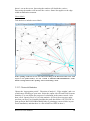
3.12. Network analysis ................................................................................. 76
3.12.1. Data selection .......................................................................... 77
3.12.2. Network Visualization ............................................................ 78
3.12.3. Network Statistics ................................................................... 79
3.12.4. Generate stochastic data .......................................................... 81
3.13. Operating the simulator via command-line ......................................... 81
4
Algorithms and user modules .................................................................... 83
4.1. Algorithms ............................................................................................. 83
4.1.1. Algorithms for RTGS systems .................................................. 93
4.1.2. Algorithms for CNS systems .................................................... 96
4.1.3. Algorithms in DNS systems...................................................... 98
4.1.4. Algorithms in DVP/PVP processing systems ......................... 100
4.1.5. Algorithms for systems with bilateral limits ........................... 101
4.2. Algorithms for special cases................................................................ 104
4.2.1. Receipt-reactive RTGS ........................................................... 104
4.2.2. Group codes for DVP linking multiple transactions ............... 107
4.3. System event handler algorithms (SEH) ............................................. 109
4.4. Time estimation algorithms (TEA) ..................................................... 109
4.5. User module interface ......................................................................... 110
4.5.1. Adding a user module ............................................................. 111
5
Data content and databases ..................................................................... 112
5.1. File directory structure ........................................................................ 112
5.2. About MySQL ..................................................................................... 113
5.2.1. MySQL Query Browser .......................................................... 114
5.2.2. MyODBC interface ................................................................. 115
5.2.3. Direct modifications of simulator database ............................ 115
BoF-PSS2 User Manual
2
5.3. Databases ............................................................................................. 116
5.3.1. Database structure ................................................................... 118
5.3.2. Database tables........................................................................ 119
5.3.3. Database table repairs ............................................................. 122
5.4. Data sets .............................................................................................. 122
5.5. Date format .......................................................................................... 123
5.6. Time format ......................................................................................... 124
5.7. Time transposition functionality ......................................................... 124
5.8. File template ........................................................................................ 125
5.9. Selection criteria .................................................................................. 126
5.10. About using Microsoft Excel with the simulator .............................. 126
6
Application screens................................................................................... 127
6.1. Main menu ........................................................................................... 127
6.2. Initial specifications ............................................................................ 128
6.3. User module definition ........................................................................ 128
6.4. System control data specification/modification .................................. 129
6.5. Import input file................................................................................... 129
6.6. View data sets ...................................................................................... 130
6.7. Delete data sets .................................................................................... 130
6.8. Export input file................................................................................... 131
6.9. Simulation configuration ..................................................................... 131
6.10. Simulation execution ......................................................................... 132
6.11. View simulation logs ......................................................................... 132
6.12. Basic statistics reports ....................................................................... 133
6.13. Account comparison .......................................................................... 133
6.14. System comparison............................................................................ 134
6.15. Delete output data .............................................................................. 134
6.16. Export output file............................................................................... 135
6.17. Network Analysis Toolbox ............................................................... 135
7
Technical documentation ......................................................................... 136
8
Troubleshooting guide ............................................................................. 136
9
Acknowledgements ................................................................................... 138
BoF-PSS2 User Manual
3
1. Introduction
The Bank of Finland Payment and Settlement System Simulator (BoF-PSS2), is
analysis software designed for payment and settlement system simulations. The
simulator can be used for studying liquidity needs and risks in payment and
settlement systems. Special situations, which are often difficult or impossible to
test in a real environment, can be simulated with this tool.
This document is the user manual of BoF-PSS2. It describes features
of the software and their use. It also provides overview of technical details of the
simulator and refers to other documentation, where more details can be found.
The manual is structured as follows.
Chapter 1 provides this introduction and describes general structure and
possible usages of BoF-PSS2.
Chapter 2 provides instructions for installation of BoF-PSS2 and necessary
third party software.
Chapter 3 presents the user interface of BoF-PSS2 and describes its
existing features.
Chapter 4 presents outline of algorithms, which are the building blocks
used in describing simulated payment systems.
Chapter 5 presents outline of data management and structure of the
database.
Chapter 6 provides screenshots of the graphical user interface.
Chapter 7 includes references to more detailed technical documentation of
the simulator.
Chapter 8 includes short troubleshooting guide
Chapter 9 lists acknowledgements of contributors, who have participated
in the development of the tool.
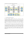
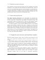
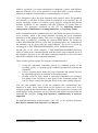
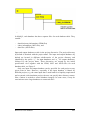
1.1. General overview
The BoF-PSS2 system structure contains three main subsystems:
a) Input generation subsystem
b) Simulation execution subsystem
c) Output analysing subsystem
BoF-PSS2 User Manual
4
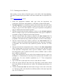
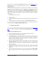
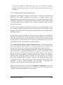
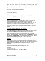
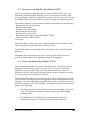
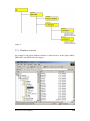
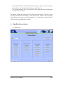
The architecture of the PSS2 program is pictured below:
1.1.1. Input generation subsystem
The input generation subsystem includes tools to import and validate
transaction data, participant data, as well as data on daily account balances and
credit limits. All data are stored in database files. The importer’s main task is to
check that the input data is formally valid and then transfer it into system database
structures. The correctness of the input data is vital. Account numbers or
identifiers in the transaction file must correspond to the account or participant
data.
All input data must be presented in CSV (comma separated values) format,
but it can be entered in a user-defined order. The input data can be edited by
exporting them from the input database as CSV files to Excel. They can then be
re-imported after the changes. (Current Excel versions can handle about 65,000
rows. If larger files need to be edited, other tools (e.g. Access or SAS) or direct
programming is usually needed. In rare situations, splitting tables in sub-tables
may be a suitable solution.) The simulator does not include a proprietary editor for
this purpose.
BoF-PSS2 User Manual
5
1.1.2. Simulation execution subsystem
The simulation execution subsystem includes tools for configuring and running
simulations. It also contains the actual simulation and settlement logic. It keeps a
log of all events and bookings and makes reports and statistics on simulation runs.
A control panel facility is available to set up and manage settlement structures,
configure settlement rules and launch, monitor and control simulation runs. The
simulator keeps a log file for the user of all simulations made.
1.1.3. Output analysing subsystem
The output analysing subsystem has the functionality for reporting basic
statistics for common result parameters. The output database contains the raw data
for the booking order of transactions and balances of settlement accounts. The
input database contains the transaction flow, while the output database contains
the settlement flow, i.e. settlement order and timing of submitted transactions.
An analyser program is used to generate additional reports. Users typically
perform many different simulations and want to compare the results of the
different runs. The analyser does some comparisons automatically, but additional
analyses may require exporting CSV files for use with tools such as Excel. It is
thus advisable to create a structure beforehand for simulation runs and determine
which results are to be stored in databases for further analysis. The databases can
become overly massive when transaction volumes are high and all transactionlevel events are retained in the databases.
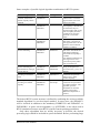
1.2. Supported system structures and simulation examples
BoF-PSS2 software supports a large variety of general system structures. It can
model most payment and settlement structures and processes found in real
systems.
The simulator supports real-time gross settlement (RTGS), continuous net
settlement (CNS) and deferred net settlement (DNS) systems. The processing
options for these systems are defined by selecting appropriate algorithms. For
example, QUE algorithms define how transactions are released from queues,
while PNS algorithms define when and how partial net settlement of queued
transactions will be invoked.
The simulator also has multi-system capabilities, whereby a large number of
interacting systems can be included in the same simulation (see chapter 3.9.4).
When transactions occur between systems, they are booked in separate
intersystem accounts. There are two types of intersystem transactions:
BoF-PSS2 User Manual
6
straightforward participant-to-participant transactions or system invoked injection
or settlement transactions between a main and ancillary system. In the
straightforward case, the sending system’s transaction data include a reference to
a receiving participant in another system. It is possible in ancillary systems to
define the end-of-day settlement system and accounts for each participant.
Intraday injections may also be defined. These transfer liquidity between the main
and ancillary system during the day according to participant needs.
Typical interacting system scenarios include:
–
–
–
Several independent RTGS systems constituting a network of systems, e.g.
TARGET,
A domestic payment system environment consisting of an RTGS system and
ancillary systems, e.g. a CNS and a DNS system settling in the RTGS system,
and
RTGS system settlement between an RTGS and a securities settlement
system.
The simulator also supports multi-currency and multi-asset processing, which
allows simulation of international payment systems and securities settlement
systems. Assets are treated as book-entry currencies. Payment-versus-payment
(PVP) and delivery-versus-payment (DVP) processing is supported. DVP/PVP
transaction pairs should be connected via a DVP/PVP-link code. In addition to
single intra-system DVP/PVP processing in RTGS or deferred net settlement
mode, the simulator also supports RTGS DVP/PVP settlement between real-time
systems.
The focal output factors in simulations are typically counterparty risk and
overall risk, liquidity consumption, settlement volumes, gridlock situations and
queuing time. Measures for these factors will be stored in the output database. In
what-if simulations, the input parameters are modified to distinguish effects on
output factors. The following input parameters are often used or modified in
simulations:
–
–
–
–
–
–
–
–
Input transaction flow (e.g. testing when a single counterparty or system has
problems),
Available liquidity,
Credit limit/debit cap restrictions,
Queuing and netting processes,
Participant behaviour due to e.g. new pricing patterns,
New settlement procedures, e.g. new algorithms,
Structural changes, e.g. the merging of several systems,
Changes in participant structure (e.g. introducing new participants, merging
old participants), and
BoF-PSS2 User Manual
7
–
New intersystem processes (e.g. a shift to RTGS-based DVP processing from
end-of-day batch processing).
Liquidity is introduced the simulations either by defining daily opening balances
and/or intraday credit limits. Liquidity can also be introduced via repotransactions and there are more alternatives available: introducing only the money
legs between the participants and the central bank account (with abundant limit),
introducing in DVP mode the money legs in the RTGS system and the asset legs
in a separate securities settlement system or having a special collateral account
(monetary value only) in the RTGS or securities settlement system.
Participant level risk management features can also be directly introduced in
simulations by using bilateral limits (bilateral debit caps). These can be defined at
bilateral and also at multilateral level separately from other liquidity
arrangements.
Simulations may use available data from current systems or fictional, but
representative, data. The simulator can be described as a deterministic model with
stochastic input.
Data for some examples are distributed with the simulator software, e.g. an
RTGS simulation, an RTGS system with an ancillary CNS or DNS system and a
real-time DVP securities settlement system. Some correct results are provided for
all examples as illustration of what can be obtained as simulation output. All
examples are available in two versions: with decimal commas and with decimal
points. The data for the examples and system descriptions are found in the
directories C:\BoF-PSS2\examples\DECIMAL_COMMA and
C:\BoF-PSS2\examples\DECIMAL_POINT.
BoF-PSS2 User Manual
8
2 Installation
Before using BoF-PSS2 software, you need to install the MySQL/MariaDB
database server. Instructions for this are given below.
Information on how to order and download the BoF-PSS2 program is posted
at www.bof.fi/sc/bof-pss.
2.1. Hardware and software requirements
Hardware
At least a PC Pentium 4 class processor with at least 1 GB of main memory is
recommended, even though the simulator can be run with less memory and a
slower processor. Sufficient main memory is essential for rapid execution of large
transaction volumes. At least 2 GB of main memory is recommended for large
simulations and 4 GB or more for very large simulations (>1,2 million
transactions and >1000 participants). Note that the 32-bit version of the Java
virtual machine is able to use only approximately 1.5 GB of memory. In order to
be able to allocate more memory than 1.5 GB to the Java virtual machine and the
simulator, 64-bit versions of the Java Runtime Environment and the simulator are
needed. Naturally the operating system also needs to be a 64-bit environment.
The BoF-PSS2 simulator can process massive transaction flows effectively
with adequate available main memory resources. The complexity of the
algorithms used and the selected output tables to be computed during the
simulations strongly influence the running times and memory usage of
simulations.
The BoF-PSS2 simulator keeps all transactions and other input data to be
processed during a simulation in the main memory. The amount of transactions is
the decisive factor in main memory use. When there are more transactions than
space in the main memory, system performance is likely to degrade strongly due
to necessary disk swaps. Even then, the simulator continues processing during
such circumstances until the limit of 1.5 GB is achieved for the 32-bit version.
Software
Windows XP/Vista/Windows 7
Microsoft Excel installed (required to open reports from the user interface)
MySQL/MariaDB/MS SQL-SERVER database server installed.
Sun Microsystem’s Java Runtime Environment (JRE) 1.7.0_09-b05 (distributed
and installed with the BoF-PSS2 program).
The BoF-PSS2 program should work with limitations in Linux, although this is
yet to be tested. Please contact the Bank of Finland if you are interested in running
the software in a Linux environment.
BoF-PSS2 User Manual
9
2.2. Installing a database server
The BoF-PSS2 program assumes that Microsoft Excel and either MySQL,
MariaDB or MSSQL Server are installed before the installation of the Simulator.
2.2.1. Installing MySQL
This chapter describes how to install MySQL database server, either one with
commercial or GPL license. Refer to the the next section if you prefer MariaDB.
The basic environment for the simulator is assumed to be a stand-alone PC or
a server in which the MySQL database is installed separately. If you employ a PC
or a server in which MySQL is already installed and used by other applications, it
is advisable to contact your in-house technical support persons or consult the
MySQL manual on multi-application parallel use.
MySQL versions tested with the simulator are 4.1 and 5.0. Installation
procedures of these two versions are identical. Necessary steps for the installation
of MySQL 5.0 are listed below. Newer versions of MySQL are not yet supported.
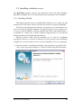
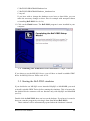
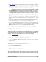
1. Extract the archive containing the MySQL setup program (e.g. mysql-classic5.0.83-win32.zip) and run Setup.exe. Click next in the Setup Wizard window.
BoF-PSS2 User Manual
10
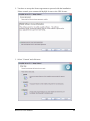
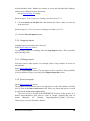
2. You have to accept the license agreement to proceed with the installation.
Please consult your commercial MySQL license or the GPL license.
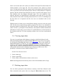
3. Select "Custom" and click next.
BoF-PSS2 User Manual
11
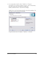
4. It is recommended to install to either C:\MySQL\ or C:\Program
Files\MySQL\. The simulator installation program is able to automatically
detect these folders and will configure the database.bat
database_shutdown.bat and C:\my.cnf files accordingly.
MySQL Server and Client Programs should be selected for installation. The
other items are not necessary for the simulator.
Using the default location for MySQL (C:\MySQL\ ) is advisable.
BoF-PSS2 User Manual
12
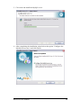
5. Click next and install the MySQL server.
6. After completing the installation wizard select the option "Configure the
MySQL Server now" and click Finish.
BoF-PSS2 User Manual
13
7. Select "Standard Configuration" and click next.
8. Unselect "Install As Windows Service" and select "Include Bin Directory in
Windows PATH".
BoF-PSS2 User Manual
14
9. Click next and execute, and the setup of MySQL is finished.
If you have problems, please consult the
http://dev.mysql.com/doc/refman/5.0/en/index.html.
MySQL
manual
at
2.2.2. Installing MariaDB
MariaDB database server offers a drop-in replacement functionality for MySQL.
It is built by some of the original authors of MySQL together with assistance of
free and open source software developers. MariaDB versions 5.2 and 5.3 (both
32bit and 64bit) are expected to work equally well as the commercial MySQL
software. Note that MariaDB version 5.5 does not yet work properly with current
release of BoF-PSS2.
Installation steps of the MariaDB database server:
1. Download the MariaDB installation utility corresponding to your
operation system from http://downloads.mariadb.org/mariadb/5.3/ . For
32-bit Windows the file name is of the format mariadb-5.3.7-win32.msi and
for 64-bit Windows it is of the format mariadb-5.3.7-winx64.msi.
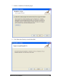
2. Double click the msi-installation file to start the installation and click Next
in the setup wizard window.
BoF-PSS2 User Manual
15
3. Accept the license to proceed with the installation and click Next.
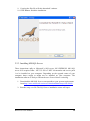
4. At the Custom Setup screen, select at least the MariaDB Server “Database
instance” and “Client Programs” to be installed. Install additional parts
according to your preference. The BoF-PSS2 setup will automatically
detect MariaDB installed in C:\MySQL though any location is acceptable.
BoF-PSS2 User Manual
16
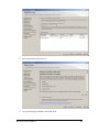
5. Untick the option “Modify password for database user ‘root’“.
6. Untick the “Install as service” option.
BoF-PSS2 User Manual
17
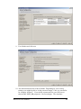
7. Enable or disable the Feedback plugin.
8. Click Next when Ready to install MariaDB.
BoF-PSS2 User Manual
18
9. Copying the files file will take about half a minute.
10. Click Next to finish the installation.
2.2.3. Installing MS SQL-Server
These instructions aplly to Microsoft’s SQL-server 2012.EXPRESS. MS SQL
server 2012 requires either .NET 3.5 SP1 or .NET 4 framworks and service pack
1 to be installed on your computer. Depending on the upgrade status of your
computer theses might or might not be installed on your computer. The
installation software is likely to inform the user if one of these is missing.
1. Download the MS-SQL Server correspondin to your system requirements
from http://www.microsoft.com/en-us/download/details.aspx?id=29062.
2. Run the setup .exe file The SQL Server installation center will open.
BoF-PSS2 User Manual
19
3. For a new installation select: New SQL Server stand-alone installation or
add features to an existing installation.
4. If your computer is connected to the internet, you might want to allow the
installer to get updates.
BoF-PSS2 User Manual
20
5. Select install new SQL-Server
6. Accept licensing conditions and click next
BoF-PSS2 User Manual
21
7. Select all features and click next.
8. Select Default instance. Set instance ID to MSSQLSERVER
BoF-PSS2 User Manual
22
9. Use defaults and click next
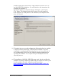
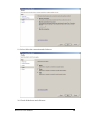
10. Set authentication mode to Mixed Mode. Depending on your security
settings you might be able to let the password empty, if not you can define
for example “bofpss2”. If you define a password here you will have to
edit the BoF-PSS2_DB.properties –file accordingly. The simulator
BoF-PSS2 User Manual
23
installer assumes the password to be empty and the user name to be “sa”
for SQL-SERVER installations. For more details see the instructions for
installing the simulator 2.3
Specify the SQL Server Administrator by clicking the “Add Current
User” button. The displayed name of the current user will most likely
differ from the one on the picture of the manual as your computers own
name will be used.
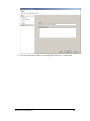
11. This guide does not cover the configuration of Reporting Services and this
is why the selection install only is selected in the example. If you feel
confortable in configuring the Reporting Services now, you can freely do
so. Note Reporting Services are not needed for running simulations nor
operating the simulator. It is a separate tool provided by Microsoft for
reporting purposes.
12. The installation of MS SQL-SERVER is now ready. In order to allow the
simulator to connect with the SQL-SERVER you will have to define a port
in to the windows Firewall. Instruction can be found from :
http://windows.microsoft.com/en-US/windows7/Open-a-port-inWindows-Firewall
BoF-PSS2 User Manual
24
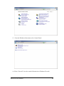
13. From the Windows Start menu select Control Panel
14. Write “Firewall” in to the search field and select Windows Firewall.
BoF-PSS2 User Manual
25
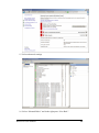
15. Select advanced settings
16. Select “Inbound Rules” and in the right pane “New Rule”.
BoF-PSS2 User Manual
26
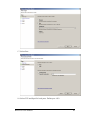
17. Select Port
18. Select TCP and Specific local ports. Define port 1433.
BoF-PSS2 User Manual
27
19. Select Allow the connection and click next
20. Check all the boxes and click next
BoF-PSS2 User Manual
28
21. Give the connection a name. For example SQL Port 1433. Click Finish.
BoF-PSS2 User Manual
29
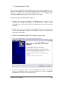
2.3. Installing BoF-PSS2
Here, we describe installing the BoF-PSS2 program using the installation wizard.
MySQL or MariaDB needs to be installed before starting the installation. You can
cancel the installation by clicking the Cancel button on the Wizard page.
Clicking the Back button brings you back to the previous page.
Installation steps of the BoF-PSS2 simulator:
1. Download the encrypted installation file delivery.exe to a folder of your
choosing, for example the Desktop or My Documents. Address of the
download page is provided by Bank of Finland after you have ordered the
simulator.
2. Double click on the .exe file you downloaded. Input the password you
received from the Bank of Finland. The installation file will be extracted and
stored in the same folder.
3. Double click extracted .exe file. The installation program starts
4. Click on the Next button. The license agreement appears.
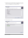
5. You have to accept the license before continuing the installation. If you can't
accept, the installation will be cancelled. Read the text, select I accept the
agreement and click then on the Next button.
BoF-PSS2 User Manual
30
6. Select the directory where the program will be installed. It is advisable to use
the default directory. Click on the Next button.
7. Don't change the default value if you want the Setup to create a folder for the
simulator in the Start Menu. If you want to use an existing folder, use Browse
BoF-PSS2 User Manual
31
to select the Start Menu folder in which you would like the Setup to create the
shortcuts for the simulator. Click the Next button.
8. Select Create a desktop icon if you want to create a shortcut icon on your
desktop. Select Create a Quick Launch icon and Setup creates an icon in the
Quick Launch menu. Click the Next button and the summary of the choices
appears.
BoF-PSS2 User Manual
32
9. On this page you see all selections made on previous pages. If you want to
change the selections, go back by clicking on the Back button. If you accept
selections, click the Install button. The installation will start.
10. Wait for the files to be copied.
BoF-PSS2 User Manual
33
11. Select the database server that you wish to use with BoF-PSS2 simulator, and
that you previously installed. The choice will affect the properties-file located
at C:\BoF-PSS2\PROGRAM\DBConnectors\BoF-PSS2_DB.properties. The
properties-file will by default specify Drizzle-connector for MySQL and
MariaDB, and Microsoft JDBC4 connector for MS SQL (See also 2.8
Changing the database connector on page 40). If you select MS SQL Server,
go to step 13 after clicking Next. Otherwise continue to step 12.
12. In case MySQL or MariaDB was selected, BoF-PSS2 will need to know
where its start-up files and databases are located. Specify the location of your
database server base and data folder. If you installed to C:\MySQL\ or
C:\Program Files\MySQL\ the fields should be filled automatically. Then,
click Next. If you can’t find these folders or some files inside these folders are
missing, make sure that MySQL/MariaDB was installed with “Client
programs” enabled in the Custom Setup screen (step 4 in MySQL/MariaDB
installation steps).
(The files affected by these path definitions are:
BoF-PSS2 User Manual
34
C:\BoF-PSS2\PROGRAM\Database.bat
C:\BoF-PSS2\PROGRAM\Database_shutdown.bat
C:\my.cnf
If you later wish to change the database server base or data folder, you can
make the necessary changes to these files for example with notepad without
re-installing BoF-PSS2. See ch 2.6)
13. Click on the Finish button. The BoF-PSS2 program is now installed in your
computer.
2.4. Running the simulator with Microsoft’s SQL Server
If you chose to use the MS SQL-Server, you will have to install a suitable JDBC
driver for MS SQL-Server. Please refer to 2.8.
2.5. Starting the BoF-PSS2 simulator
If you decided to use MS SQL-server instead of MySQL or MARIADB, you need
to install a suitable JDBC Driver before running the simulator. This is because the
the default Drizzle connector will not function only with MySQL and MariaDB
(see 2.8).
Double click the BoF-PSS2 short-cut icon on the desktop. If you haven’t created a
short-cut, start the program by selecting it from Start Menu (BoF-PSS2).
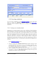
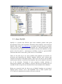
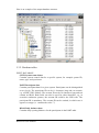
Three windows will be automatically opened when the simulator is started:
BoF-PSS2 User Manual
35
1. The start up.bat sequence window. This window shows information of
simulator status and e.g. displays error messages if there are problems
with connection to MySQL/MariaDB or in the java runtime environment.
Contents of this window are written to c:\BoF-PSS\Program\log.txt
2. The MySQL monitor window opens since the MySQL server is started
automatically.
3. Simulator application and user interface window itself.
When the simulator is installed, the system database (c:\BOFPSS2\PSS2_systemdb) is not yet created. When the simulator is started, it will
check if it can find the system database, if not it will create it. Later, if for a
reason or an other, the simulator will not be able to find the system database, it
will try to recreate it. The first session, equivalent to a situation when operating
with a blank system database with no projects defined, will require that you
specify a first project. The project information defines the location of databases
and reports, see 3.3 for details.
After stating a name for the project, (e.g. example1) click on the file fields and the
default values will appear. Save the project information by clicking on the "save
project modification" button. Return to the main menu and your simulator
installation is completed.
2.6. Starting and closing database server
The MySQL/MariaDB database monitor has to be up and running before
launching the simulator. This simulator’s startup.bat sequence automatically
launches and closes MySQL/MariaDB.
If the simulator was installed with MS SQL SERVER the rows for starting
databases are left out from the bat-files. MS SQL SERVER runs as a service on
the background and thus will not need to be started separately unless it has been
explicitly shut, when it would have to be started manually from Control Panel->
System and Security -> Administrative Tools -> Services
If you experience problems at these phase, it might be due to a missconfiguration.
Normally the simulator’s installation program will configure the necessary bat and
cnf files autoamtically. But you might want to check this. If you installed the
MySQL (or MariaDB) for example in c:/MyDB/ , the files should look like in the
following examples:
the C:/my.cnf file should include the following lines:
[mysqld]
BoF-PSS2 User Manual
36
basedir = D:/ MyDB /
datadir = D:/ MyDB/data/
C:\BOF-PSS2\PROGRAM\Database.bat
@echo off
title MySQL
echo on
"C:\MyDB\bin\mysqld-nt" --defaults-file=c:\my.cnf --console
exit
C:\BOF-PSS2\PROGRAM\Database_shutdown.bat
echo off
"C:\MyDB\bin\mysqladmin.exe" -u root shutdown
exit
Starting MySQL/MariaDB independently
MySQL/MariaDB are versatile database servers. You can find information about
them at www.mysql.com and mariadb.org.
MySQL databases created by the simulator can also be accessed directly for
exporting or importing data or performing minor changes in the databases (e.g.
delete unnecessary templates, projects or system names). Caution, however, is
needed when making direct modifications. Direct usage of MySQL is described in
more detail in 5.2.
2.7. Run time performance and start-up parameters
Run time performance of the simulator is largely dependent on the amount of
memory available for the simulator, MySQL/MariaDB database and the operating
system. In large simulations, insufficient or badly allocated memory leads to
paging, where hard disk is used as an extension for main memory.
The memory allocations for simulations are controlled with two parameter
files: one for the simulator and one for MySQL/MariaDB database. If you
experience lengthy run times or make changes to hardware configuration of your
simulator PC you might want to change these configurations to see if there is
some positive impact. Remember that also too large buffer reservations may slow
down processes if the memory being left for other applications is insufficient
BoF-PSS2 User Manual
37
Simulator start-up parameters
The simulator itself is a Java application and it is run in a Java virtual machine.
The parameters of Java are defined in the start-up script of simulator in file
C:\BoF-PSS2\PROGRAM\Start-up.bat. This file contains a code line starting the
Java virtual machine and setting, inter alia, the memory limits for it.
The code line starts with command "jre-1.7\bin\java" and continues with two
memory parameters: –Xms***m and –Xmx***m. Here –Xms sets the amount of
memory given for the simulator applications directly at start-up and –Xmx sets the
maximum amount of memory that can be given for the application. The asterisks
*** represent the amount of memory in megabytes.
The memory parameters of Java virtual machine in startup.bat are
automatically scaled by the installation program according to the amount of main
memory in the PC or server. The code lines in different setups are by default the
following:
1. "jre-1.7\bin\java –Xms64m –Xmx512m …
less of main memory
2. "jre-1.7\bin\java –Xms128m –Xmx512m …
3. "jre-1.7\bin\java –Xms192m –Xmx1024m …
4. "jre-1.7\bin\java –Xms256m –Xmx1408m …
" if the PC has 256MB or
" if … 512MB
" if … 768MB
" if … 1GB or more
If the amount of memory in simulator PC is decreased after installation or the
memory parameter values are too large for other reasons the simulator start-up is
cancelled and error message is displayed in the start-up window saying "Could
not reserve enough space for object heap". In this situation the -Xmx parameter in
the file BoF-PSS2\PROGRAM\Start-up.bat must be changed to a smaller value.
The currently used 32-bit Java Runtime Environment version 1.7 (since BoFPSS2 v3.2.1) is capable of using a maximum of 1.7 GB of memory. This
restriction is imposed by the limitations of the 32 -bit memory address space and
operating system architecture. 64-bit hardware, operating systems and Java
Runtime Environment allow a considerable increase, so that the limit of the
maximum memory will more likely be restricted by the hardware and the amount
of memory on the computer.
MySQL/MariaDB start-up parameters
Parameters for controlling MySQL/MariaDB database performance are given in
configuration file c:\my.cnf. Four versions of configuration files are included with
the simulator for different hardware configurations. These configuration files are
BoF-PSS2 User Manual
38
located at C:\Bof-PSS2\PROGRAM\. The installation program selects
automatically one of these files to be used and copies it to my.cnf according to the
amount of main memory in the PC or server. If a c:\my.cnf –file has been created
already earlier, it is renamed to my_old.cnf. Selection rules are the following:
1. MySim-256M.cnf if the PC has 256MB or less of main memory
2. MySim-512M.cnf if the PC has 512MB of main memory
3. MySim-768M.cnf if the PC has 768MB of main memory
4. MySim-1G.cnf if the PC has 1GB or more of main memory
The configuration files contain following parameters.
Wait_timeout is the number of seconds the database server waits for activity
on a open connection before closing it. To make sure that database connection
is not closed in very large and long lasting simulations this parameter is raised
from default 28800 (8 hours) to 3153600 (one year in seconds).
Key_buffer_size determines the cache size available for database table
indexes. This is the most important buffer in MySQL/MariaDB and the value
is recommended to be 25- 50% of main memory reserved for
MySQL/MariaDB.
Join_buffer_size determines the memory reserved for queries to multiple
tables. This could have approximately 5% of all memory reserved for
MySQL/MariaDB.
Read_buffer_size determines memory reserved for reading tables. This is
also recommended to be 5% of memory reserved for MySQL/MariaDB.
Sort_buffer_size is reserved for sorting tables. Recommended size also 5%.
Tmp_table_size determines the size of temporary table that can be held in
memory.
Recommended size 10-5% of all memory reserved for
MySQL/MariaDB.
Myisam_sort_buffer_size determines the memory reserved for sorting in
database maintenance and defragmentation functions. Size equalling 5-10% of
memory reserved for MySQL/MariaDB is adequate. Note however that this
parameter does not affect the run time performance of database.
Table_cache determines the number of tables that can be open
simultaneously. This is set to the number of tables in one simulator project and
does not need to be changed.
The values and combination of start-up parameters can be changed in the my.cnf
file. The configuration files provided with the simulator are modified versions of
configuration files found in the standard MySQL/MariaDB distribution. These are
located in c:\mysql directory with names like my-small.cnf and my-huge.cnf, and
can also be used to learn more about MySQL/MariaDB start-up commands. A
BoF-PSS2 User Manual
39
complete list of parameters and their definitions are available in the MySQL
manual (chapter 5.2.3).
2.8. Changing the database connector
A JDBC driver is a software component enabling a Java application to interact
with a database via the JDBC interface. The default JDBC driver used by BoFPSS2 is Drizzle JDBC, a BSD-licensed native java JDBC driver for Drizzle and
MySQL. The Drizzle database connector is located in C:\B oFPSS2\PROGRAM\DBConnectors \DrizzleJDBC.jar.
The user may wish to use another database connector. This can be done by
copying the corresponding jar-file to DBConnectors folder and editing the lines in
text file C:\B oF-PSS2\PROGRAM\DBConnectors\BoF-PSS2_DB.properties.
The default connector is defined by the lines:
DBConnectorFile=DrizzleJDBC.jar
JDBC_DRIVER=org.drizzle.jdbc.DrizzleDriver
DB_URL=jdbc:drizzle://localhost/
If you are eligible to use GPL software, you can download a GPL MySQL
connector from http://dev.mysql.com/downloads/connector/j/ . Similarly, if you
have a commercial license for the MySQL connector you can use your licensed
connector. Copy the corresponding driver file e.g. mysql-connector-java-5.1.21bin.jar
or
mysql-connector-java-commercial-5.1.7-bin.jar
to
C:\BoFPSS2\PROGRAM\DBConnectors. Then in BoF-PSS2_DB.properties file located
in the same folder, comment the default connector lines using “#” and define the
new connector according to the lines below:
If your connector file is mysql-connector-java-5.1.21-bin.jar
DBConnectorFile=mysql-connector-java-5.1.21-bin.jar
JDBC_DRIVER=com.mysql.jdbc.Driver
DB_URL=jdbc:mysql://localhost/
or if your connector file is mysql-connector-java-commercial-5.1.7-bin.jar
DBConnectorFile=mysql-connector-java-commercial-5.1.7-bin.jar
JDBC_DRIVER=com.mysql.jdbc.Driver
DB_URL=jdbc:mysql://localhost/
In practice, during the testing of the simulation we have observed no difference in
using different connectors. However, the BoF-PSS2 now includes the possibility
to use any JDBC-connector. In particular DrizzleJDBC and the GPL/commercial
MySQL connector are known to work with BoF-PSS2.
BoF-PSS2 User Manual
40
If you chose to use the MS SQL-Server, you will have to install a JDBC driver for
MS SQL-Server. We recommend to use MICROSOFT JDBC DRIVER 4.0 FOR
SQL SERVER. The driver can be found from Microsoft’s downloading center (
http://www.microsoft.com/en-us/download/details.aspx?id=11774 . The driver
should be copied to c:\BOF-PSS2\PROGRAM\DBConnectors\ ). The installation
program of the simulator configures the c:\BOFPSS2\PROGRAM\DBConnectors\BoF-PSS2_DB.properties file automatically to
function with this driver if the corresponding selection was made during the
installation. Still it is good to check that the connection strirngs of the properties
file do contain the same port, user name and passwords that you defined for the
MS SQL-SERVER before.
The file should have the following rows active (not preceded by #):
DBConnectorFile=sqljdbc4.jar
JDBC_DRIVER=com.microsoft.sqlserver.jdbc.SQLServerDriver
DB_URL=jdbc:sqlserver://127.0.0.1:1433;
DB_USERNAME=sa (depending on the defined user namewhen installing SQLServer)
DB_PASSWORD=
(If your securioty settings allowed you to let the
password undefined, else you should define the same password)
BoF-PSS2 User Manual
41
3 Operating the BoF-PSS2 simulator
This chapter describes BoF-PSS2 screens and how to use them.
3.1. Short description of BoF-PSS2 simulator use
The simulation process is normally divided into distinct phases.
You begin by specifying the systems you want to simulate. This includes
stating the system name, setting the open hours, and selecting the processing
logics and algorithms that are used in a system, see 3.4.
Next, you import input data for the system just specified into the input
database (participant names and transactions and optionally daily opening
balances, intraday credit limits and bilateral balances), see 3.5.
Once you have specified the system structure and input data, you configure
simulations in the Simulation configuration screen and cross-check data sets
belonging to the simulations, see 3.9.
Simulations are executed by accessing the Simulation execution screen, see
3.10. You can run one or more simulations at a time.
After running the simulations, you can export reports, compare simulations,
and delete or export output data, see 3.11. Reports can be saved in CSV files.
These files can be further analysed and processed outside the simulator.
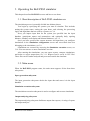
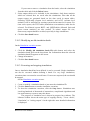
3.2. Main menu
When the BoF-PSS2 program starts, the main menu appears. Select from three
subsystems:
Input generation subsystem
The input generation subsystem checks the input data and stores it in the input
database
Simulation execution subsystem
The simulation execution subsystem is used to configure and execute simulations
Output analysing subsystem
The output analysing subsystem facilitates output data exports, viewing of reports
and output analyses.
BoF-PSS2 User Manual
42
Network analysis system
The network analysis system can be used to generate networks (graphs) from
input or output transaction data and then to calculate statistics from the generated
networks.
The user is directed to Initial specifications screen the first time the program
is run in order to establish the first project. This project becomes the default
project until new projects are defined. This will be prompted automatically during
the first session. Read more on projects below.
3.2.1. Project
Select a project from the drop-down list on the main menu. The default project is
the last selected project.
The simulator uses the definitions of the selected project until you select a
new project, see 3.3. A project can be changed only from the main menu.
Projects separate the input and output data of different simulation projects
(e.g. RTGS simulations from CNS simulations), allowing the same input data and
the input database to be used. Generally, it is advisable to use the default directory
layout.
3.2.2. Main menu buttons
The main menu provides access to sub-functions. The user must follow a logical
order in the simulation process. First, load the necessary input data, then define
the simulations to be executed, and finally set the results to be analysed. The
process is often iterative, which leads to new input data requirements and
additional simulations.
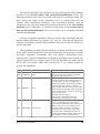
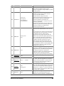
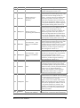
Screen / Button to open
Initial specifications
Purpose
You can add new projects and modify old ones
User module definitions You can define your own modules
You can import input data from files
Import input file
Define system data
You can update or create system data
View data sets
You can view information of all data sets
Delete data sets
You can delete data sets
Export input file
You can export input data into files
Simulation
You can cross-check data sets and configure a
BoF-PSS2 User Manual
43
configuration
simulation
Simulation execution
You can execute simulations
View simulation logs
You can view simulation logs
Basic statistics reports
You can view basic statistics reports of simulations
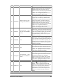
Account comparison
You can analyse simulations at the account level by
making comparisons
System comparison
You can analyse simulations at the system level by
making comparisons
Delete output data
You can delete output data
Export output file
You can export output data into files
Generate networks
You can generate network data from transaction
data in input or output databases.
Analyse networks
You can calculate certain statistics from the
generated network files.
Generate stochastic
data
Automatic generation of transaction and participant
data using a generation algorithm.
Help
You can open the help
Exit program
You can stop the program by clicking the Exit
program button
3.3. Working with projects
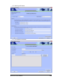
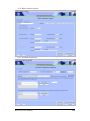
The Initial specifications screen opens, when you start the BoF-PSS2 program
for the first time.
Create a new project or modify old ones on this screen. The screen can be
opened later by clicking the Initial specifications button on the Main menu.
Each project has its own directory that carries the project name. The project
name can be up to eight characters long. Special characters should be avoided, but
underline (_) is acceptable. Under this directory following sub-directories are
created:
–
–
–
–
–
–
Input database directory,
Output database directory,
Default directory where input files are located,
Default directory where error lists are saved,
Default directory where output files are saved, and
Default directory where output reports are saved.
BoF-PSS2 User Manual
44
The location of each directory can be edited before creating the project. Default
directories for other than input and output database can also be edited for existing
projects.
The proposed default location of new project and all of its subfolfers can be
defined by editing DefaultProjectPath variable in c:\BoF-PSS2\PROGRAM\BoFPSS2.properties file.
You can change the default project on the Main menu.
The basic idea of project definitions is to separate the input and output databases
for different simulation projects. Especially the output database can become very
large if all simulations over a longer time are saved in the same database. The
simulations will be faster when databases are kept moderate in size. It will also be
easier to make back-ups, when databases are smaller.
3.3.1. Creating a new project
Projects can be created for different types of projects using different input data
and creating different output data. It is easy to destroy unnecessary data when it is
organised according to projects. This is especially useful when projects create
large databases and file directories.
On the Initial specifications screen:
1. Click the Create new project radio button and type in the name of the project
(up to eight characters). The program proposes input and output names and
default directories. You can change them, but be careful! For example, you
can name an existing database to share input data, but still keep the output
databases separate.
2. Click the Save project modification button. The project will be saved and
become vivible in the drop-down list in the Main menu.
If a project folder already exists with the corresponding name, the files,
including the database files, in the project folders will not be over written.
Only the necessary information according to the selections will be stored in
the PSS2_ systemDB.
3.3.2. Modifying an old project
On the Initial specifications screen:
BoF-PSS2 User Manual
45
1. Click the Modify old project radio button and choose a project from the
drop-down list. Information of the selected project is shown in the fields of
the screen.
2. Change the project information. Be especially careful when changing
database specifications.
3. Click the Save project modification button.
3.3.3. Project duplicates and backups
All data which is defined or created in a simulation project is stored in the folder
of this project. This makes it possible to easily backup and restore or duplicate
projects.
As an example a project with name "example1" on PC 1 is considered. Its folder
is located at C:\BoF-PSS\p_example1. Contents of this project can be transferred
to an another computer, PC 2, including all imported data, specified systems,
results from executed simulations and created reports in the following way:
1. In PC 2, which has BoF-PSS2 ready and installed, a new project is created
with same name as the copied: example1. The location of this project
folder is assumed to be D:\BoF-PSS\p_example1.
2. Simulator software is closed on both PC:s
3. The folder C:\BoF-PSS\p_example1 from the original PC is copied and
used to replace the folder D:\ BoF-PSS\p_example1 of the newly created
namesake project in the second PC.
After this the simulator can be started in PC 2 and the contents of example1project can be used and studied further as in PC 1.
Similarly backups can be made of simulation projects. The same procedure can
also be used for transferring only some parts of the projects such as input
database. The overall file and directory structure of the simulator is presented in
more detail in chapter 5.1.
NOTE! The major version number of the simulator in both computers has to be
the same. When changes in the database structure of BoF-PSS are made, the first
number in the version numbering is increased e.g. from version 1.2.0 to 2.0.0.
This makes it impossible to transfer databases by simply copying the files. Also,
the installed MySQL/MariaDB versions should be the same on both PC's.
BoF-PSS2 User Manual
46
3.3.4. Deleting projects
Projects that are no longer needed can be deleted to release disk space. This can
be done by using the delete project feature on the Initial Specifications screen by
selecting the relevant project from the old projects list and by prssing the Delete
Project button at the bottom right corner.
Projects can also be removed manually.Removing a project by simply deleting a
project folder and all of its contents, may lead to problems. Necessary steps for
deleting a project manually are described below, while instructions for direct use
of MySQL are given in chapter 5.2.
Note that there is also possibility to decrease the size of existing simulator
projects by deleting unnecessary input data or output results and by optimizing the
database respectively. This can be done simply with the simulator user interface,
see chapters 3.7 and 3.11.11.
For deleting a project with name "RemoveMe" do the following steps. Note that
the only project in existing BoF-PSS2 installation should not be deleted. If you
need to delete the only project, create a new empty project to remain as the default
project before proceding.
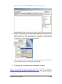
1. Close BoF-PSS2 and open preferred tool for directly editing MySQL
database. MySQL Query browser is used in these instructions (see chapter
5.2).
2. Select PSS2_systemdb by double clicking the database name in schemata
on the right.
3. Remove the line related to the project to be deleted from PROJ table. This
can be done e.g. by executing a query:
BoF-PSS2 User Manual
47
delete from proj where SP_PROJEID='name_of_the_project';
4. Delete the definitions of input and output databases of the project from
MySQL by right clicking the database name from schemata and selecting
"Drop Schema". In this example these are Schemas i_RemoveMe and
o_RemoveMe. Confirm deletion for each database.
5. After changes in database contents, the entire project folder can be deleted
from the simulator folder C:\BoF-PSS\P_RemoveMe.
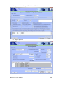
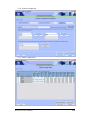
3.4. Setting up a payment and settlement system
Create a new system data set or modify an old system data set by accessing the
System control data specification/modification screen. The screen opens by
clicking the Define system data button on the Main menu. This screen is used to
BoF-PSS2 User Manual
48
define available system names and system data sets: settlement conventions and
algorithms for the systems. The use of parallel system data sets for the same
system facilitates simulations with the same transactions and participants, but
different processing patterns or methods.
The system control data specifications contain the basic system information for
each system to be simulated.
3.4.1. Creating a new system data set
On the System control data specification/modification screen:
1. Select correct system ID for the new system data set from drop down list. If
the desired system ID is not available, click Create new system ID radio
button and type in the system ID. It is recommended to use the name of the
real system under study as the system ID.
2. Click the Create new system data set radio button and type in the name of
the data set.
3. If you want to copy from an old system data set, click Copy from old system
data set button. When you select a system data set from the drop-down list,
information of the data set appears in the system data fields. You can change
this information. Delete old algorithms and introduce new algorithms or
change their parameter values.
4. System full name, system acronym and system description are optional
information
5. Opening and closing hours are mandatory. The cross-check function is
checking that the input data is within these limits. The values of open and
closing hours must be between 00:00 and 24:00. If the simulated system is
open over midnight, time transposition can be used. See chapter 5.7 Time
transposition functionality.
6. System type (RTGS, CNS or DNS) is mandatory and directs which
algorithms will be available in the potential algorithm window.
7. Transfer balances to next day can be used in multi-day simulations for
transferring the end-of-day balances to become the beginning-of-day balances
for the next day.
8. If the simulated system includes bilateral limits, the bilateral limits in use
option has to be selected. After this, algorithms designed for handling bilateral
limits will be available in step 11 of system definition. See 4.1.5 Algorithms
for systems with bilateral limits. This selection only affects the visiblilty of
the algorithms in the selection list.
BoF-PSS2 User Manual
49
9. Intraday credit availability requires a choice between three options. The
selection 'Credits according to limit table' requires an ICCL dataset
containing the intraday credit limits to be defined. 'No credits available'
indicates that only the liquidity on accounts is available. This means that only
a DBAL data set is needed. The last option 'credit available without limits'
indicates that overdrafts are freely available. This option can be used to find
out the upper bound of liquidity. Note that liquidity has to be provided in
some form, otherwise no transactions will settle.
10. Handling of unsettled transactions has four options. All unsettled
transactions will be kept in a special queue for unsettled transactions until the
end-of-day and the processing will be dependent on the selected option.
Transfer unsettled transactions to next day/settlement occasion will place
unsettled transactions back in the transaction queues to be settled later if
possible. Delete unsettled transactions (include in statistics) will remove the
transactions from queue but still include them in output statistics and reports.
Delete unsettled transactions (exclude from statistics) means that the unsettled
transactions will be removed from queue and also from all transaction level
statistics and most system and account level statistics. They will only be
included in aggregate transaction value and transaction count numbers in
system and account level statistics. Force end-of-day settlement will result in
bookings on the accounts irrespective of any credit limit violations. This can
lead to negative account balances at end of day. Forced end-of-day settlement
can be used to find out the minimum liquidity needed to settle all transactions
at least at the ends of the day. An account violation record (AVST) will be
written for every violating transaction.
11. Select the appropriate algorithms. Algorithms define the processing
methods. Entry ENT and END end-of-day algorithms are mandatory for all
systems. Select an algorithm and fill in its parameter values, when required.
Add it to the attached algorithms by clicking on the Add algorithm button.
See 4.1 Algorithms for details. Selected algorithms can be removed by
selecting the corresponding row on pressing the keyboard's delete button.
12. The version 3.0.0 allows the use of time estimation algorithms (TEA). A TEA
-algorithm can be associated to an algorithm and used to approximate the real
duration of given algorithm run. This allows replication of precesses where
settlement algorithms or processes are executed in parallel. A time estimation
algorithm can be added by double clicking the field after which the system
opens a new time estimation algorithm definition view. The public algorithms
which are available in the general 3.0.0 version of BoF-PSS2 do not currently
support time estimation, but this feature can be used in user modules. Support
for TEA will likely increase in the future according to demand.
13. Click the Save system data set button.
BoF-PSS2 User Manual
50
3.4.2. Modifying an old system data set
You may want to change the information in an old system data set, for example, if
there are errors in the first version.
1. Click Select existing system ID radio button and select the correct system ID
from drop down list
2. Click the Modify old system data set radio button and select the name of the
data set from the drop-down list. Information about the selected system data
set appears in the system data fields.
3. To change information, first delete old algorithm(s) and introduce new
algorithm(s) or change parameter values.
4. Click the Save system data set button.
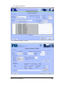
3.5. Importing data
You can import data from files to the input database by accessing the Import input
file screen. The screen opens by clicking on the Import input file button on the
Main menu.
You can import participant data, daily balances data, intraday credit limits data,
transaction data and bilateral credit limit data by means of this screen. System
data can be defined on the System control data specification/modification screen.
The input file has to be a text file, e.g. .txt or .csv. You also have to specify data
and decimal separators and date and time formats.
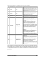
The different input data types/data tables are coded as follows:
–
–
–
–
–
PART contains participant and account data. This can be defined on
participant level only or alternatively on combined participant and account
level. In the latter case, the same participant may have multiple accounts, but
for each both the participant and account ID should be specified. This feature
can be used to define different omnibus accounts for clearing parties in a
securities settlement system.
DBAL contains the initial daily balances data of participants or accounts. It is
optional, and lacking processing, starts from zero balances the first day.
ICCL contains intraday credit limit changes of participants. It is also optional.
TRAN contains the transactions of a given system. There can also be
transactions pointing to other systems. This is done by defining the 'tosystem' field for transactions. The 'from-system' field must always contain the
same ID, which is defined as the system ID of the dataset.
BLIM contains the bilateral limits between pairs of participants. It is optional.
BoF-PSS2 User Manual
51
–
–
RSRV contains information on reservations. Reservations are used to reserve
a specific amount of the available liquidity to be used to settle some specific
type of transactions. Support for reservations is algorithm specific and for the
moment there are no built in algorithms in the generally available version of
BoF-PSS2 which support the use of reservations. Reservations data can be
used in own user modules. For the availability RSRV supporting algorithms
you should check with the simulator team. There can be many different
reservations defined for one account.
SYCD contains system control data. These data must be specified for each
system. This specification is done in the System control data specification –
screen, not by importing a dataset.
A system ID has to be defined for each imported data table. It is used when
searching and configuring data that belongs to the same system. System ID is
selected from a drop down list, which includes all system IDs that have been
defined in the system definition window, see chapter 3.4.
Multiple data sets can be used for running the simulations with varying input
data. This is facilitated by a data set ID specified for each data table. The input
database will thus contain parallel data sets with the same information, e.g.
different data sets for intraday credits to simulate a situation with varying
liquidity. There may also be different transaction flows depicting e.g. crisis
situations. To manage a large number of parallel data sets effectively, it is
important to create a consistent naming convention. The data set ID can be up to
eight characters long.
It is important to note that the input systems only check the data content at the
field level. Due to possibility of multiple parallel data sets, cross-checking can
only be performed after simulations are configured and parallel data sets selected.
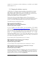
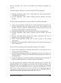
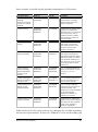
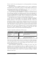
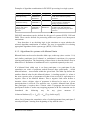
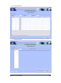
Templates are used for inputting data using CSV files. The templates
describe the data field order in the CSV files.
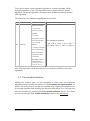
The templates specify in which order to input data fields are in the input CSV-file
(see example below).
BoF-PSS2 User Manual
52
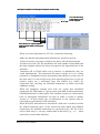
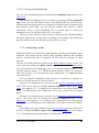
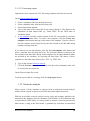
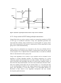
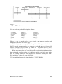
Example of CSV-file and Import template relationship
Two introductory
explanation rows
to be skipped
File column in input template
tells the data order in the input
CSV-file
When you create input data in a CSV file, consider the following:
–
–
–
–
–
–
Make sure that the data and decimal delimiters are specified correctly.
Values of currency can only be stated to two places after the decimal point.
All data rows in the CSV-file should have the same number of data fields and
the input template defines how these correspond to the input data base of the
simulator.
Transaction ID in TRAN tables can be numeric or alphabetical, they are
sorted alphabetically. The transaction ID must be unique as it is a sorting
parameter to distinguish between transactions that otherwise would occur in
the same order. It is also used as a key when reporting input errors. If you use
numeric values, use a sufficiently large first number (e.g. 10001) for
transaction files involving ten thousand transactions to assure successful
alphabetic sorting.
When the simulation contains more than one system and interlinked
transactions the TRAN data of a given system must hold all debit transactions
(FROM-transactions) of that system. The simulator operates on credit transfer
basis so intersystem transactions can only be made as credits to another
system (i.e. all direct debit type of transactions in real systems must be
converted to credit transfers in the simulator.)
When DVP/PVP transactions are introduced a link code is needed to define
the linked transaction pairs. If the system has both linked and unlinked
transactions, the unlinked transactions are specified in the CSV-file with a
null or blank entry i.e. an entry without data in that field (e.g. ;; or ; ; when
semicolon is used as data delimiter).
BoF-PSS2 User Manual
53
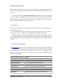
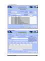
3.5.1. Creating a new data set
The creating of a new data set function stores a new table in the input database.
The table is defined by its given data set ID and contains data in a specified CSV
file.
On the Import input file screen:
1. Select the appropriate database table type from the drop-down list
(participant, transaction, daily balances, credit table or bilateral limit table).
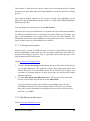
2. The data separator is a mark that separates data fields from each other in the
CSV file. The last selected separator is shown in the field. If you wish to
change it, type in a new data separator. Any type of separator is acceptable as
long as it differs from the decimal separator.
3. The last selected input decimal separator is shown in the decimal separator
field. To change it, type in a new decimal separator. Any type of separator is
acceptable as long as it differs from the data separator.
4. The last selected input date format is shown in the date format field. To
change it, select a new one from the drop-down list. Any type of separator is
acceptable. The dash does only symbol its position. See also 5.5 Date format.
5. The last selected input time format is shown in the time format field. To
change it, select a new format from the drop-down list. Any type of separator
is acceptable. The colon does only symbol its position. See also 5.6 Time
format.
6. The last selected time transposition value is shown in the time transposition
field. Transposition can be used to increase or decrease time and date values
in the input data. Transposition value is given in ±hhmm –format. In import
the transposition value is added to all time values (in DBAL values a whole
day is added or subtracted).
Using Time transposition can be useful if the simulated system is open over
midnight, i.e., if transactions for one day in the system do not fit inside a real
calendar day. For more detailed explanation see 5.7 Time transposition
functionality.
7. Type in the name of the input file or select it with ‘Browse’ button.
8. Select the system ID from drop down list. Only those system names which
have been defined for this project are visible. For defining system names, see
chapter 3.4.
9. Click the Create new data set radio button and type in the name of the data
set. The data set ID is the identifier for different tables of the same input data
type. See 5.4 Data sets.
BoF-PSS2 User Manual
54
10. A file template describes which columns in the file correspond to particular
fields in the database table. If you want to create a new template, click the
Create new template radio button and type in the template name. Type
ordinal numbers in the first column in the data table on the screen.
Templates are stored so that if you want to use an old template, click the
Use old template radio button and select a template from the drop-down list.
The selected template is shown in the first column of the data table. Again, a
consistent naming convention is helpful. Old templates can also be modified
after they are selected. The changes are saved when a modified template is
used.
11. Type in the Number of rows/records to skip at the beginning field the
number of rows at the beginning of the file not to be imported (e.g. header
rows).
12. Type in the Number of rows/records to skip at the end field the number of
rows at the end of the file not to be imported (e.g. summary rows).
13. Click the Execute import button. Rows from the file will be imported and
stored in the selected database table. You can control the number from the
Rows processed window, as well as the Rows with errors window.
Items 2-6 in the above list are together referred to as the data format defaults.
3.5.2. Updating an old data set
Updating an old data set will update the given fields defined by the template in the
specified data table for rows where the keys of the data table and the input CSV
file match. Other rows remain untouched. Key fields cannot be updated.
On the Import input file screen:
Perform steps 1–8 as in creating a new data set in chapter 3.5.1.
9. Click the Update old data set radio button and select a data set from the
drop-down list.
Perform steps 10–13 as in creating a new data set in 3.5.1.
12. Click the Execute import button.
3.5.3. Inserting data in an old data set
The inserting function provides the possibility to add rows into an existing data
table defined by the data set ID. Rows without matching keys are inserted into the
BoF-PSS2 User Manual
55
selected database table. Matches are treated as errors and discarded (the database
content is not changed in these situations).
On the Import input file screen:
Perform steps 1–8 as if you were creating a new data set in 3.5.1.
9. Click the Insert in old data set radio button and select a data set from the
drop-down list.
Perform steps 10–13 as if you were creating a new data set in 3.5.1.
12. Click the Execute import button.
3.5.4. Stopping import
Lengthy import processing can be aborted.
In the Import input file screen:
To stop import while it is running, click the Stop import button. This is possible
only with large files.
3.5.5. Undoing import
You may want to undo imports, for example, when a large number of errors are
encountered.
In the Import input file screen:
Click the Undo import button. The last import will be cancelled. This possibility
is only available as long as you stay on the Import input file screen.
3.5.6. Errors in import
On the Import input file screen:
The program checks that the data to be imported are valid. The number of faulty
rows is seen in the Rows with errors field. Errors are listed and may be viewed
by clicking the View error report button.
The error list file is located in the ERRORLIST directory of the project. It is
named ImportInputError_date_time.csv (date in format yymmdd and time in
format hhmmss), for example, ImportInputError_090407_121030.csv.
Unnecessary error lists should be deleted.
BoF-PSS2 User Manual
56
In the error list the row refers to the row number in the input file and the col to the
column number in the input file. The most common errors found are format
errors. For date and time fields the formats used in the imported file should be the
same as specified in the data format defaults. Numeric fields should be completely
numeric and the decimal sign should be the same as stated in the import screen.
The simulator does not support 'thousand' signs. The error 'duplicate entry'
indicates that there are duplicated key information in the input file e.g. two rows
with transaction data with coinciding transaction IDs. In case of coinciding keys
the first data row is imported and the next ones are discarded with an error
message.
Different kind of format errors and delimiter changes can arise when the input
CSV file has been exported from another program, like Excel. It is advisable to
check the content of exported CSV files with a software showing the true content
of the CSV file e.g. Notepad. Check delimiters, date and time formats and decimal
information, because there seems often to be small differences in these details if
the simulator and the CSV data exporting software have not been synchronized
earlier.
3.6. Viewing input data
You can view participant, daily balances, intraday credit limit, bilateral credit
limit and transaction data sets with the View data sets screen. This screen opens
by clicking the View data sets button on the Main menu. This is only suitable for
small and moderate size data sets. For transaction data only the first 10 000 rows
of data set will be shown. The export input file function is available to check
larger data sets. MySQL database can also be accessed and even modified directly
with suitable software such as MySQL Query Browser or MS Access. This
possibility is described in more detail in chapter 5.25.2.
On the View data sets screen:
1. Select a data type.
2. Select a system ID.
3. Select a data set ID and data is shown on the screen.
Note! Searching transaction data may take a while if the database table is large.
3.7. Deleting input data
You can delete participant, daily balances, intraday credit limit, bilateral credit
limit, transaction and system data sets using the Delete data sets screen. The
BoF-PSS2 User Manual
57
screen opens by clicking the Delete data sets button on the Main menu. The
Delete data sets screen is also helpful in giving a view of the data sets stored in
the input database.
The disk size of the input database is not decreased when data sets are deleted. For
that purpose the input database needs to be optimized or defragmented after the
deletion. This can be done by clicking the optimise input database button. For
large databases this can be a lengthy process. Optimization of database will also
improve the simulator performance if you have made large number of database
modifications.
On the Delete data sets screen:
1. Select data type.
2. Select system ID; all data sets of the given data type and system appear on the
screen.
3. Select the data sets to be deleted and click on the Delete data sets button.
4. If several data sets have been deleted and the disk size of simulator data needs
to be decreased, click optimise input database button.
3.8. Export input file
You can export data from the input database to files by accessing the Export input
file screen. The screen opens by clicking the Export input file button on the Main
menu.
On the Export input file screen:
1. Select the database table type to be exported from the drop-down list.
2. Select a data set ID from the drop-down list.
3. The data separator is a mark that separates data fields from each other in the
output CSV file. The last selected value is shown in the field. To change it
type in a new data separator. Any type of separator is acceptable as long as it
is different from the decimal separator.
4. The last selected decimal separator for the output CSV file is shown in the
decimal separator field. If you want to change it, type in a new decimal
separator. Any type of separator is acceptable as long as it is different from
the data separator.
5. The last selected date format for the output CSV file is shown in the date
format field. To change it, select a new one from the drop-down list. See also
chapter 5.5.
6. The last selected time format for the CSV file is shown in the time format
field. To change it, select a new one from the drop-down list. See also chapter
5.6.
BoF-PSS2 User Manual
58
7. The last selected time transposition value is shown in the time transposition
field. The transposition value is given in ±hhmm format. In export the
transposition value is subtracted from all time values (in DBAL values a
whole day is subtracted or added). This means there is no need to change the
sign of transposition value given in the input phase. For more detailed
explanation see 5.7 Time transposition functionality.
8. Type in the name of the output file. The default directory is INPUT.
9. Select the Create names of columns field when you want the names of the
columns to appear in the output file.
10. A file template describes which columns in the output file should correspond
with particular fields in the database table. To create a new template, click the
Create new template radio button and type in the name of the template. Type
ordinal numbers into the first column of the data table. If you leave empty
columns in the templates, these will appear as two adjacent separators in the
output file.
To use an old template, click the Use old template radio button and
select a template from the drop-down list. The selected template is shown in
the first column of the data table.
11. Type in selection criteria and select the parts of the table you want to export.
Selection criteria can be written for each data field.
12. Click the Execute export button. Data from the selected database table will
be exported to the output file. The number of rows appears in the Rows
processed window.
To abort export while it is running, click the Stop export button.
The selection criteria facilitates exports of subsets of the imported input tables eg
in order to edit some of the data with Excel.
3.9. Setting up simulation runs
You can create a new simulation ID, modify an old simulation ID or cross-check
data sets on the Simulation configuration screen. The screen opens by clicking
the Simulation configuration button on the Main menu.
3.9.1. Creating a new simulation ID
Each simulation must have a specific simulation ID of up to eight characters. Use
a consistent naming convention to avoid troubles.
On the Simulation configuration screen:
BoF-PSS2 User Manual
59
1. Click the Create new simulation ID radio button and type in the simulation
ID. If you want to copy from an old simulation, click the Copy from old
simulation ID button and select a simulation ID. Information from the old
simulation ID appears on the screen and can be changed.
2. Type in the name of the simulation and the description. These fields are
optional.
3. Select SUB submission algorithm from the drop-down list. Parameters of the
selected algorithm are shown in the Parameters box. Double click the box
and type in the parameter values.
4. The most important task is to select the systems and their data sets to be
included in the simulation. First select a system ID from the first drop-down
list. Next, select data sets from the other drop-down lists. System, transaction
and participant data sets are mandatory. Only systems with all mandatory data
sets available can be configured, i.e. are shown in the selection window.
Credit limit and daily balances data sets are optional. Add the selected values
of the drop-down lists to the table by pressing the Add/update data set
button.
If you want to change a row in the table, select the system ID from the
drop-down list, change the data sets you want and press the Add/update data
set button.
If you want to delete a row from the table, select it from the table and
click the Delete button.
5. Click the Save simulation ID button.
3.9.2. Modifying an old simulation ID
Old simulation IDs may need to be modified, for example, in the case of errors in
earlier specifications. When the simulation ID is modified, the old output data is
destroyed.
On the Simulation configuration screen:
1. Click the Modify old simulation ID radio button and select a simulation ID
from the drop-down list. Information about the selected simulation ID appears
on the screen.
2. Change information.
3. Click the Save simulation ID button.
BoF-PSS2 User Manual
60
3.9.3. Cross-checking data sets
Cross-checking verifies that the information in selected data tables (data sets) is
coherent, e.g. all accounts needed are available for booking transactions,
intraday-credit changes are within transaction dates and opening hours and initial
balances are within transaction days.
It is good practice to run a cross-check when a configuration is created.
During cross-check the number of errors found is shown. The progress of crosscheck is displayed by telling which simulation ID, system ID and data sets are
currently checked. The progress-bar window tells also, at suitable intervals, which
row in the first table is under processing by showing the transaction ID or
participant ID.
To stop a cross-check, press the Stop cross-check button.
If the cross-checking finds errors, they may be viewed by clicking the View
errors button. The error list file is located in the ERRORLIST directory of the
project. It is named SimulationConfigurationError_date_time.csv (date in format
yymmdd
and
time
in
format
hhmmss),
for
example
SimulationConfigurationError_090407_121030.csv. Unnecessary error lists
should be deleted.
The error list contains a reference to the incoherent input data record and
information about the missing relationship data. The dataset ID and a short
description will be shown for each error.
Typical cross-check errors are
- Date errors: the dates in DBAL, BLIM or ICCL tables are outside the
simulation dates, i.e. dates for which transactions are specified in the TRAN
table. Limits and balances should only be defined for those days which are
simulated.
- Time errors: the transaction introduction times specified in the TRAN table
are outside the opening hours of the simulated system, as defined in system
data.
- Participant errors: there are missing participants (or typing errors) in the
participant data. TRAN-PART refers to transactions with missing participants
in PART data, DBAL-PART refers to missing participant data for DBAL data
and ICCL-PART refers to missing participant data for ICCL data. For all
participants quoted in TRAN, ICCL, BLIM and DBAL records there must be
the corresponding participant in the PART data. If multiple systems or
accounts are defined, the participant is checked as a combination of the system
ID, participant ID and account ID.
BoF-PSS2 User Manual
61
-
Erroneous system ID's in TRAN data: if the from system id field is explicitly
defined, it should be the same as the ID of the system which this data set is
attached to.
3.9.4. Creating multi system simulations
Simulations with multiple interacting systems can be created and simulated with
BoF-PSS. This enables simulation and analysis of parallel systems with
independent processing logics, such as network of several RTGS systems such as
TARGET, combination of a RTGS system and an ancillary CNS or DNS system
or a RTGS payment system together with a securities settlement system working
with DVP processing.
In multi system simulations individual systems are set up independently one by
one: system definition and data imports are performed for each simulated system
separately. System ID field is used to collect together definitions and input data of
individual systems.
For transactions between systems the receiving system name has to be defined in
input data. Transactions are always included in transaction data set of that system,
where the from-participant of each transaction is located. The system names used
in input data (e.g. From-system and To-system in transactions) need to be the
same which are used as System IDs in system definition.
The transaction IDs must be unique simulation-wide, i.e. the transaction data
sets of the different systems cannot use same transaction IDs. Cross-check will
display reused IDs as errors of the second transaction data set that uses them.
An example of multi system simulation is provided in example2 material included
with the simulator (C:\BoF-PSS2\EXAMPLES). It presents a main RTGS system
and an ancillary CNS using the accounts in the RTGS system as the source of
liquidity. In the input data the "liquidity injections from system" and "liquidity
injections from participant"-fields are defined for each participant. In the input
data of this example the RTGS system is referred as "M" and the ancillary system
is referred with "K". These names have to be used also as System IDs in the
simulation. In multi system simulations, the cross-check is checking also
coherency of multi system transactions and used System IDs.
Multi system simulations are created in simulation configuration screen by
including all necessary systems one by one on their own rows. Screenshot from
example 2 simulation configuration is shown below.
BoF-PSS2 User Manual
62
3.10. Executing simulations
You can execute simulations on the Simulation execution screen. The screen
opens by clicking the Simulation execution button on the Main menu.
Simulations can be executed as single runs or in batches consisting of many
simulations.
3.10.1. Creating a new simulation batch
Simulations are executed in batches of one or more simulations. Stored simulation
batch information is convenient, particularly when a large number of simulations
need to be reprocessed. Output data is also defined with this screen. By creating
and saving a simulation batch, the selections made in this screen can be stored for
future use. Simulations can also be executed without saving the batch run
information (skip steps 1 and 4 below). When exiting the window, a warning will
be displayed of unsaved data. This does not refer to the output data you select to
include in simulations in step 3. It will always be stored when the simulations are
executed.
On the Simulation execution screen:
1. Click the Create new simulation batch ID radio button and type in the
simulation batch ID. If you want to copy an old simulation batch ID, select
the simulation batch ID from the drop-down list. Information about the
selected simulation batch ID appears on the screen.
2. Select a simulation ID from the drop-down list and add it to the simulation
batch table by clicking the Add simulation ID button. Repeat this step for all
simulations you want to execute in same batch.
BoF-PSS2 User Manual
63
If you want to remove a simulation from the batch, select the simulation
from the table and click the Delete button.
3. Select output tables to be included in the simulations. Only those statistics
which are selected here are saved after the simulations. Note that all the
output reports are generated based on the data saved in output tables.
Selecting SYLS-table (System level statistics) and ACST (account level
statistics) will be sufficient for creating system and account level reports. For
time series reports, the TEST-table (transaction event statistics) must also be
selected. For bilateral reports BIST- and QURE-tables (bilateral limit and
queue reason statistics) are also needed. To reduce output file size,
unnecessary output should be avoided, especially in large simulations.
4. Click the Save batch button.
3.10.2. Modifying an old simulation batch
On the Simulation execution screen:
1. Click the Modify old simulation batch ID radio button and select the
simulation batch ID from the drop-down list. Information about the selected
simulation batch ID appears on the screen.
2. Change information.
3. Click the Save batch button.
3.10.3. Executing and stopping simulations
Once a simulation batch has been defined, it can be executed. Single simulations
can also be executed without defining a batch. For very large simulations,
execution times can extend to several hours. If errors are suspected, the run should
be stopped.
On the Simulation execution screen:
1. Create or modify a simulation batch or just enter the simulation ID.
2. Click the Start button to start the simulation execution.
3. To abort the simulation execution, click the Stop button. Simulation runs
involving hundreds of thousands of transactions, complicated algorithms and
low main memory resources may take hours.
The progress of simulation run is shown in progress bar windows. The
leftmost window shows the main type of ongoing activity: "Cross- check",
"simulation" or "writing output". On the right side more detailed information
is displayed.
BoF-PSS2 User Manual
64
The contents of the progress bar during cross-check are described in
3.9.3. During simulation execution the simulation ID and current date and
time in the simulated environment are shown. Date and time formats in
progress bar are YYYY-MM-DD hh:mm:ss.000). In the beginning of each
simulation text "initializing" is shown instead of time during start-up period.
While writing output the time is replaced with the name of output table being
written.
For small simulations the easiest way is just to select the right simulation
ID, required output tables and click on the Start button. The batch option is
convenient when making a large number of simulations by changing for
example some parameters in the input data.
3.10.4. Skip/execute cross-check
Execute cross-check is the default value. It is advisable to cross-check the data in
the start of every simulation. However, a skip cross-check feature is introduced,
which can be used on user's risk. This is provided to speed up very large
simulations, where the cross-check is slow and when the user is sure that there are
no cross-check errors in the data (i.e. the same data-sets have been cross-checked
earlier).
Skip cross-check is selected by clicking on the radio button.
The risk is that there may still be a cross-check error in the data and the simulation
result will be unexpected. In fatal cases (e.g. missing participant ID in PART data)
the simulation will stop. In non-fatal cases (e.g. credit line for dates outside the
transaction dates) the results/statistics will be incorrect and unpredictable. Other
irregularities may also occur, because the cross-check has been designed to find
these kinds of errors.
3.10.5. Errors in simulations
On the Simulation execution screen:
View errors arising in the simulations by clicking the View error report button.
The error list file is located in the error list directory of the project. It is named
SimulationExecutionError_date_time.txt (date in format yymmdd and time in
format hhmmss), for example, SimulationExecutionError_090407_121030.csv.
Unnecessary error lists should be deleted.
BoF-PSS2 User Manual
65
3.10.6. Viewing simulations logs
You can view simulation logs by pressing View simulation logs button on the
Main menu.
Logs of all run simulations may be viewed by accessing the View simulation
logs screen. The log will indicate when each simulation ID was executed most
recently and what output tables were selected to be stored in this execution. In the
last columns of the table, you can find the number and values of settled
transactions. When a given simulation ID is executed again or reused the
information stored in simulation log will be overwritten.
The logs can be sorted to desired order by clicking on the column headings.
An arrow indicates the sorting order (ascending or descending). By clicking on
the same heading once more the sorting order will be reversed.
3.11. Analysing results
Simulation results are stored in the output database according to simulation output
selections. The output can be viewed using available statistics and reporting
features. All data can also be exported via CSV files for analyses in other
software.
You can view basic statistics reports on the Basic statistics reports screen. The
screen opens by clicking the Basic statistics reports button on the Main menu.
You may select from six report types, see 3.11.1 System statistics reports, 3.11.2
Account statistics reports, 3.11.3 Bilateral limits statistics report, 3.11.4 System
time series reports, 3.11.5 Account time series reports and 3.11.6 Bilateral limits
time series report.
You can compare simulations at the system or account level. Reports are
saved as CSV files and can be viewed in Excel.
System level comparisons are accessed via the System comparison analyser
screen. The screen opens by clicking System comparison button on the Main
menu. See chapters 3.11.7 Creating a new comparison view at the system level
and 3.11.8 Modifying an old comparison view at the system level for further
details.
Account level comparisons are accessed via the Account comparison analyser
screen. The screen opens by clicking the Account comparison button on the
Main menu. See chapters 3.11.9 Creating a new comparison view at the account
level and 3.11.10 Modifying an old comparison view at the account level further
details.
Delete data from output database on the Delete output data screen. The screen
opens by clicking the Delete output data button on the Main menu. See chapter
3.11.11 Deleting data from output tables for further details.
BoF-PSS2 User Manual
66
Export data from the output database on the Export output file screen. The
screen opens by clicking the Export output file button on the Main menu. See
chapter 3.11.12 Executing export for further details.
Reports can only be produced for data tables that have been stored in the
output database according to selections made in the execution phase.
3.11.1. System statistics reports
The system statistics report provides essential system level output data for the
simulation.
On the Basic statistics reports screen:
1.
2.
3.
4.
Select a simulation from the drop-down list.
Type in the name of the output file.
Select the System statistics report radio button.
Click the Save in csv-file or Save and open csv-file button. Both actions will
save the report as a CSV file; the Save and open csv-file will open the file in
Excel.
The report contains following columns.
Col
1
2
3
4
Name
Date
System
Tot bod balances
AVG Cred Lim
5
6
7
8
Value settl
Value unsettl
Number settl
Number unsettl
Description
Date of simulation format (YYYYMMDD)
ID of system.
Sum of the balances of each account at the beginning of the day
Time weighted average of the credit limits (field Y_AVGCRLIM from
SYLS)
Sum of the transaction values of settled transactions during the day
Sum of the transaction values of the unsettled transactions during the day.
Count of the settled transactions
Count of the unsettled transactions
Note that there might be some empty fields in the system statistics when the data
tables required for calculations have not been saved. Note also that in multicurrency simulations the account data will be added together on system level
although these might be in different currencies. The information can then only be
used to check that the total turnover is technically correct.
BoF-PSS2 User Manual
67
3.11.2. Account statistics reports
The account statistics report contains the basic statistics at account level for a
specified system. For multiple day simulations account statistics are presented for
each day in ascending order.
In the Basic statistics reports screen:
1.
2.
3.
4.
5.
Select a simulation from the drop-down list.
Type in the name of the output file (use a consistent naming convention).
Select the Account statistics report radio button.
Select a system ID from the drop-down list.
Click the Save in csv-file or Save and open csv-file button. Both actions will
save the report as a CSV file; the Save and open csv-file will open the file in
Excel.
The report contains following columns.
Col
1
3
4
5
6
7
8
9
10
Name
date
Participant
Account
Bod
Eod
Ave
Min
Max
Average cred lim
11
12
13
14
Value settl
Value unsettl
Number settl
Number unsettl
Description
Date of simulation format (YYYYMMDD)
ID of participant.
ID of account.
Balance at beginning of day
Balance at end of day
Time weighted balance during the day
Minimum balance during the day
Maximum balance during the day
Time weighted average of the credit limit (field A_AVGCRLIM from
ACST)
Sum of the transaction values of settled transactions during the day
Sum of the transaction values of the unsettled transactions during the day.
Count of the settled transactions
Count of the unsettled transactions
3.11.3. Bilateral limits statistics report
The bilateral limits statistics report can only be created for simulations where the
bilateral limits in use selection has been made in the system dataset. See 3.5.1.
This report shows basic statistics for each day and each bilateral pair of
participants or accounts. The values reported relate to that specific bilateral
connection i.e. just the data between two participants.
Note! This report can become huge if the number of participants/accounts in the
simulation is large.
BoF-PSS2 User Manual
68
To create the report, follow these steps in the Basic statistics reports screen:
1.
2.
3.
4.
5.
Select a simulation from the drop-down list.
Type in the name of the output file (use a consistent naming convention).
Select the Bilateral limits statistics report radio button.
Select a system ID from the drop-down list.
Click the Save in csv-file or Save and open csv-file button. Both actions will
save the report as a CSV file; the Save and open csv-file will open the file in
Excel.
The report contains following columns.
Col
1
2
3
4
5
6
7
8
9
10
11
12
13
14
15
16
17
18
19
20
21
22
23
24
25
26
Detailed name
Simulation date
System ID
Participant ID
Account ID
Receiving in system
Receiving participant
Receiving account
Value submitted
Value settled
Value unsettled
Value received
Number submitted
Number settled
Number unsettled
Number received
End-of-day balance
Description
Date of simulation format (YYYYMMDD)
ID of system.
ID of participant.
ID of account.
ID of receiving system
ID of receiving participant. *MULTILIMIT indicates multilateral limit.
ID of receiving account
The bilateral volume submitted.
The bilateral volume settled
The bilateral volume unsettled
The bilateral volume received
The bilateral number of submitted transactions
The bilateral number of settled transactions
The bilateral number of unsettled transactions
The bilateral number of received transactions
The day’s ending bilateral balance (a sending surplus is a negative
balance).
Average limit during the day. Average limit during the day calculated from the BLIM table
Minimum limit
Minimum limit during the day calculated from the BLIM table
Maximum limit
Maximum limit during the day calculated from the BLIM table.
Average balance during the
Average bilateral balance during the day (a sending surplus is a negative
day.
balance).
Minimum balance
Minimum bilateral balance during the day (a sending surplus is a
negative balance).
Maximum balance
Maximum bilateral balance during the day (a sending surplus is a
negative balance).
Maximum queue value
Maximum queue value during the day in this particular bilateral
relationship, sender's view i.e. the largest value in queue at any time.
Calculated based on TEST and QURE table. Only values of payments,
which have been queued due to bilateral limits, are reported here.
Number of queued
Number of queued transactions per day in this particular bilateral
transactions
relationship, sender's view. Calculated based on TEST and QURE table.
Only values of payments, which have been queued due to bilateral limits
are reported here.
Total value of queued
Total value of queued transactions per day in this particular bilateral
transactions
relationship, sender's view. Only values of payments, which have been
queued due to bilateral limits, are reported here.
Total time when limit
The total time during the simulation day when the bilateral limit has been
effective
effective (format hhhhmmss000, where 000 denotes milliseconds) i.e. the
time during which one or more transactions have been in the bilateral
BoF-PSS2 User Manual
69
queue in this particular bilateral relationship. Calculated based on TEST
and QURE table.
All values are calculated from the sending participant's/account's side. For
example, when net value of payments sent between participants B1 and B2 is 100,
that is B1 has paid 100 units more to B2 than it has received payments from B2,
the value of the bilateral End of day balance (column 16) on the row, that has B1
as the sending participant (column 3) and B2 as the receiving participant (column
6) is -100 and represents a sending surplus.
If receiving participant is reported as *MULTILIMIT, this means that values in
that row represent the net position of the current participant/account towards all
the others.
More information of using bilateral limits is presented in section 4.1.5 Algorithms
for systems with bilateral limits.
3.11.4. System time series reports
The system time series report gives the opportunity to derive system-level
balances and other numeric information for given points of time as time series are
based on equal intervals in minutes.
On the Basic statistics reports screen:
1. Select a simulation from the drop-down list.
2. Type in the name of the output file. The default output directory is
OUTPUT_REPORTS.
3. Select the System time series report radio button.
4. Select a system ID from the drop-down list.
5. Type in interval in minutes (1-60) into the edit box.
6. Click the Save in csv-file or Save and open csv-file button. Both actions will
save the report as a CSV file; the Save and open csv-file will open the file in
Excel.
The system time series report is calculated as the sum of the individual
participant/account time series. The report contains following fields:
Col
1
2
3
4
Detailed name
Simulation date
Beginning of period
End of period
Liquidity available
5
Value submitted
BoF-PSS2 User Manual
Description
Date of simulation. Presented according to date format defaults
Starting time of reported time series period
End time of time series period
Aggregate value of available liquidity of all participants/accounts in the
system. Recorded at the end moment of corresponding period.
Aggregate value of all transactions submitted in the system during the
period
70
6
7
Value settled
Value in queue
8
9
10
Number submitted
Number settled
Number in queue
11
Number of participants with
transactions in queue
Aggregate value of all transactions settled in the system during the period
Aggregate value of all transactions that were in the queue during the
period. It does not matter for how long transactions stayed in the queue.
Number of all transactions submitted in the system during the period
Number of all transactions settled in the system during the period
Number of all transactions that were in the queue during the period. It
does not matter for how long transactions stayed in the queue.
Number of participants in the system with one or more transactions in the
queue during the reported period.
3.11.5. Account time series reports
The account time series report gives the possibility to derive account balances and
other numeric information at given points of time as the time series are based on
equal intervals (in minutes).
In the Basic statistics reports screen:
1. Select a simulation from the drop-down list.
2. Type in the name of the output file. The default directory is
OUTPUT_REPORTS.
3. Select the Account time series report radio button.
4. Select a system ID from the drop-down list.
5. Type in interval in minutes (1-60) in the edit box.
6. Select an account ID from the drop-down list.
7. Click the Save in csv-file or Save and open csv-file button. Both actions will
save the report as a CSV file; the Save and open csv-file will open the file in
Excel.
The report contains following fields:
Col
1
2
3
4
5
Detailed name
Simulation date
Beginning of period
End of period
Balance
Credit limit
6
Liquidity available
7
Value submitted
8
Value settled
9
Value in queue
10
Number submitted
11
Number settled
BoF-PSS2 User Manual
Description
Date of simulation. Presented according to date format defaults
Starting time of reported time series period
End time of time series period
Participant / account balance at the end of corresponding period.
Credit limit value of the participant / account at the end of corresponding
period.
Value of available liquidity of the participant / account at the end of
corresponding period.
Aggregate value of all transactions submitted in the system during the
period by this participant / account.
Aggregate value of all transactions settled in the system during the period
by this participant / account.
Aggregate value of all transactions of this participant that were in the
queue during the period. It does not matter for how long transactions
stayed in the queue.
Number of transactions submitted in the system during the period by this
participant / account.
Number of transactions settled in the system during the period by this
participant / account.
71
12
Number in queue
Number of transactions of this participant that were in the queue during
the period. It does not matter for how long transactions stayed in the
queue.
3.11.6. Bilateral limits time series report
The bilateral limits time series report allows the user to derive statistics on the
bilateral positions between a given participant and all others at given points of
time as a time series. The reporting interval is given in minutes. This report will
be available only for simulation IDs in which the bilateral limits in use –selection
has been selected in system definition.
In the Basic statistics reports screen:
1. Select a simulation from the drop-down list.
2. Type in the name of the output file. The default directory is
OUTPUT_REPORTS.
3. Select the Bilateral limits time series report radio button.
4. Select a system ID from the drop-down list.
5. Type in interval in minutes (1-60) in the edit box.
6. Select participant / account ID from the drop-down list. This will be the from
account in the bilateral calculation reported.
7. Click the Save in csv-file or Save and open csv-file button. Both actions will
save the report as a CSV file; the Save and open csv-file will open the file in
Excel.
The report contains the bilateral limit and the current bilateral balance (end-of –
time slot), the number and value of submitted and settled transactions for this pair
of participants/accounts during the time slot as well as the number and value of
queued transactions. Only transactions queued for the reason of bilateral limits
will be reported
*MULTILIMIT as the receiving participant indicates multilateral values i.e. value
calculated as a sum over all receiving participants. Queue statistics reported under
*MULTILIMIT will include the transactions queued due to the multilateral limit.
Contents of this report are defined similarly as in the bilateral limits statistics
report. See 3.11.3. More information of using the bilateral limits is presented in
the section 4.1.5 Algorithms for systems with bilateral limits.
Note! This report can become huge if the number of participants/accounts in the
simulation is large.
BoF-PSS2 User Manual
72
3.11.7. Creating a new comparison view at the system level
Comparison views provide the opportunity to compare the output of different
simulations. Simulations and data fields must be defined to be compared. This
function can be used for reporting the results from different simulations as
columns in a common table. The percentage and absolute difference compared
with the first column/simulation can also be shown. Data are saved in CSV files
for further analysis. Comparable statistics include all fields, which are recorded in
system statistics output table (SYLS). For detailed definitions of the individual
indicators, see Description of BOF-PSS databases and files document.
On the System comparison analyser screen:
1. Select the Create new comparison view radio button and type the name of
the comparison view. To copy from an old comparison view, select a
comparison view from the drop-down list. Information of the selected
comparison view is shown on the screen.
2. Type in the name of the output file. The default directory is
OUTPUT_REPORTS.
3. If you want the differences from the first selected simulation to be displayed,
select the Show percentage or Show absolute check-box, or both.
4. Add simulations, systems and fields to the comparison report.
Adding: Select a value from the drop-down list and add it to the table by clicking
the Add to comparison button.
Deleting: Select the row to be deleted from the table and click the Delete button.
5. Click the Save in CSV file or Save in CSV file and open button. Both
actions save the report as a CSV file; the Save in CSV file and open action
also opens the report in Excel.
3.11.8. Modifying an old comparison view at the system level
On the System comparison analyser screen:
1. Select the Modify old comparison view radio button and select a comparison
view. Information about the selected comparison view is shown on the screen.
2. Type in the name of the output file.
BoF-PSS2 User Manual
73
3. To see the differences from the first selected simulation, select the Show
percentage or Show absolute check-box, or both.
4. If desired, change the comparison condition.
Adding: Select a value from the drop-down list and add it to the table by clicking
the Add to comparison button.
Deleting: Select the row to be deleted from the table and click the Delete button.
5. Click the Save in CSV file or Save in CSV file and open button. Both
actions will save the report to a CSV file; the Save in CSV file and open
action also opens the file in Excel.
3.11.9. Creating a new comparison view at the account level
The account comparison view compares output data at the account level. The list
of comparable statistics includes all fields, which are recorded in the account
statistics output table (ACST). For detailed definitions of the individual indicators,
see the Description of BOF-PSS databases and files document.
On the Account comparison analyser screen:
1. Select the Create new comparison view radio button and type the name of
the comparison view. If you wish to copy from an old comparison view, select
a comparison view from the drop-down list. Information about the selected
comparison view appears on the screen.
2. Type in the name of the output file.
3. If you want to display differences with the first selected simulation, select the
Show percentage or Show absolute check-box, or both.
4. Add simulations and fields to the comparison report. Select system ID from
the drop-down list.
Adding: Select a value from the drop-down list and add it to the table by clicking
the Add to comparison button.
Deleting: Select the row to be deleted from the table and click the Delete button.
5. Click the Save in CSV file or Save in CSV file and open button. Both
actions save the report as a CSV file; the Save in CSV file and open action
also opens the file in Excel.
BoF-PSS2 User Manual
74
3.11.10. Modifying an old comparison view at the account level
On the Account comparison analyser screen:
1. Select the Modify old comparison view radio button and select a comparison
view. Information of the selected comparison view is shown in the screen.
2. Type the name of the output file.
3. To see the differences from the first selected simulation, select the Show
percentage or Show absolute check-box, or both.
4. If desired, change the comparison condition.
Adding: Select a value from the drop-down list and add it to the table by clicking
the Add to comparison button.
Deleting: Select the row to be deleted from the table and click the Delete button.
5. Click the Save in CSV file or Save in CSV file and open button. Both
actions save the report as a CSV file; the Save in CSV file and open action
also opens the file in Excel.
3.11.11. Deleting data from output tables
The output database needs cleaning up from time to time. A good practice is to
delete unnecessary data as soon as possible. The disk size of the output database is
not decreased when data sets are deleted. For that purpose the database needs to
be optimized or defragmented after the deletion. This can be done by clicking the
optimise output database button. For large databases this can be a lengthy
process. Optimization of database will also improve the simulator performance if
you have made large number of database modifications.
On the Delete output data screen:
1. To delete an entire simulation, click the Remove entire simulation column as
selected. If you want to delete only output statistics, click the statistics tables
you wish to delete and select.
2. Click the Delete output data button.
3. If several data sets have been deleted and the disk size of output database
needs to be decreased, click optimize output database button.
BoF-PSS2 User Manual
75
3.11.12. Executing export
Output data can be exported in CSV files using templates and selection criteria.
On the Export output file screen:
1.
2.
3.
4.
Select a simulation ID from the drop-down list.
Select a database table from the drop-down list.
Select data format defaults.
Type in the name of the output file if you want to change it. The default is the
simulation id dash output table e.g. "Sim8-TEST" for the TEST-table of
simulation Sim8.
5. A file template describes which columns in the file correspond to particular
fields in the database table. To create a new template, click the Create new
template radio button and type in the name of the template. Type the order of
the data columns in the output file into the first column of the data table using
numbers starting from one.
If you want to use an old template, click the Use old template radio button and
select a template from the drop-down list. The selected template is shown in the
first column of the data table. Ready-made templates for all output database tables
are included in the simulator for exporting all data fields. The names of these
templates are the table name followed by -ALL e.g. TEST-ALL.
6. Type in the optional selection criteria.
7. Click the Execute export button. Data from the selected database table will
be exported to the output file.
On the Export output file screen:
To abort export while it is running, click the Stop export button.
3.12. Network analysis
Since version 3.3.0 the simulator is equipped with an improved network analysis
toolkit, which is based on the Java Universal Network/Graph Framework.
With the new toolkit, network analysis can be easily and instantly applied to the
transaction data imported into the simulator (TRAN table) or the transaction data
of a simulation (TEST table). It is also possible to analyse a network generated by
other means, as long as the data format is qualitatively equivalent to transaction
BoF-PSS2 User Manual
76
data and can be imported into the TRAN or TEST table by the import
functionality of the simulator or by other means e.g. direct use of SQL commands.
The network analysis toolkit can be used to create visualization of a network and
to calculate generally used network indicators
3.12.1. Data selection
Follow these steps to select the data used for network visualization and network
statistics. At this point the data should be present either as a TRAN table in in the
input database or TEST table in the output database.
Input data table / Output data table:
Select the ‘input data table’ or ‘output data table’. Select your SystemID and
DatasetID or SimulationID. When the latter is selected, the simulator
automatically fetches the data to ‘Begin date’,’End date’,’Begin time’ and ’End
time’ boxes. This can take a moment depending on the size of your data.
(If the dates and times will not appear, make sure that the data is in the correct
format.)
‘Begin date’,’End date’,’Begin time’ and ’End time’:
These dates and times affect the time window used in the visualization, and only
the date affects the date window used in network statistics calculation.
Dates and times should be entered in the same format as they appear in the
database tables TRAN/TEST. For dates this format is yyyymmdd. For times the
default format is hhmmss000000, where 000000 denotes microseconds. There is
some flexibility with the time format, less so with the date format.
SQL filter
It also possible to restrict the network to transactions according to any logical
combination of other fields in the TRAN/TEST table. The restriction will apply to
both network visualization and network statistics. Standard SQL syntax is
supported.
Examples of conditions that can be entered into SQL filter:
input data:
T_TRANVALU>1e6
T_TOPARTID=’Bank1’ OR T_FRPARTID=’Bank1’
T_TRANCLAS=1.2
output data:
BoF-PSS2 User Manual
77
E_TRANVALU>1e6
E_TOPARTID=’Bank1’ OR E_FRPARTID=’Bank1’
E_SETTSTAT=0
3.12.2. Network Visualization
Edge width (Gross value/net value/count) and Edge type (Directed/Undirected)
For the ‘Directed’ edge type the edges are arrows, for the ‘Undirected’ the edges
are line segments.
Gross value: (Directed) One edge is aggregated transaction volume in onedirection, and the width of the edge is proportional to the volume. (Undirected)
The edge is the sum of aggregated volume in both directions.
Net value: (Directed) One edge is bilaterally netted transaction volume between
two nodes, direction given by the direction of the net flow. (Undirected) Same as
directed but without the direction.
Vertex size
Gross throughput: The radius of each vertex is proportional to the sum of absolute
values of transaction in and out of the vertex.
Connections: The radius of each vertex is proportional to the number of
connections to other vertices.
Betweennes/Pagerank: The radius of a vertex is proportional to the centrality of
the vertex as defined by the indicator.
Vertex layout
Four different automatic layouts of vertices are supported. Circle layout arranges
the vertices around a circle in alphabetic or numeric order. Three other layouts
arrange the nodes based on the links between them. See the JUNG 2.0.1. API for
more information about different layouts:
http://jung.sourceforge.net/site/apidocs/edu/uci/ics/jung/algorithms/layout/packag
e-summary.html
Edge size normalization constant and Vertex size normalization constant
These optional constants can be used to scale up or down the width of edges or
size of vertices to please the eye, or in order to visualize different networks or the
same network at different times using equivalent scales so that the visual
differences can be directly compared.
For example, if the vertex size is according to throughput, the vertex size
normalization constant is a vertex throughput, for which the vertex size would be
BoF-PSS2 User Manual
78
about 1 cm on the screen. Increasing the number will shrink the vertices.
Decreasing the number will increase the vertices. Same idea applies to the edge
width normalization constant.
Vertex labels
Tick the box to include vertex labels.
In the "picking" mode the arrows are colored according to the direction of the arrow with
respect to the picked node(s). Use the "Switch to PICKING/TRANSFORMING" mode
button to change between the "picking" and "transforming" mode.
3.12.3. Network Statistics
Choose the ‘Aggregation period’, ‘Direction of analysis’, ‘Edge weights’ and a set
of indicators according to your taste. Select the output-xlsx-file and click Generate
Statistics. You can follow the progress of calculation in the status console. After
done, click ‘Open in Excel’ to view the statistics. (If Excel does not start, make
sure that you have Excel installed and that the path that follows “SET PATH” in
Start-up.bat in BoF-PSS2\PROGRAM folder is pointing to correct folder in your
Excel installation, and that there is a file called Excel.EXE in there.)
BoF-PSS2 User Manual
79
Aggregation Period (Day/Week/Month/Year)
Choose how frequently the statistical indicators are calculated.
Direction of Analysis (Inward/Outward/Undirected)
These settings can be used to adjust the network to which the indicators are
applied. Unless you absolutely know what you are doing, it is recommended to
used the standard ‘Outward’ direction.
Inward: Changes the direction of each arrow in the graph before calculating the
statistics.
Outward (recommended): Calculates the indicators using standard directed graph.
Undirected: Calculates the indicators using undirected graph.
Edge weights (None/Gross value/Net value)
These settings can be used to adjust the weights of the network to which the
indicators are applied much the same way as the ‘Edge width’can be chosen in the
visualization. Additionally, there is possibility to choose weight ‘None’, which
neglects any counts and volumes of transactions and is only concerned with
relations between the vertices. Indicators marked with * are affected by the
weights.
Indicators:
The toolbox supports a number of network indicators that are part of JUNG 2.0.1.
and a couple of additional indicators ‘Connectivity’,‘Eccentricity’ and
’Reciprocity’. Following is a short description of each indicator. Technical details
of indicators can be found in network literature and:
http://jung.sourceforge.net/site/apidocs/edu/uci/ics/jung/algorithms/scoring/packa
ge-summary.html
Barycenter (G): Inverse of sum of distances to other nodes.
Closeness(G): Inverse of average distance to other nodes.
Betweenness(G): How many shortest paths go through this node. If a shortest path
is not unique, the score is divided by the corresponding factor. For example, if
there are three shortest paths from A to F (say A->B->E, A->C->E and A->D->E)
and one unique shortest path from G to H: G->B->H, then node B gets score
1.3333333=0.3333333+1 .
Connectivity(L): Number of links divided by number of other nodes.
BoF-PSS2 User Manual
80
Clustering coefficient(G): Tells if the neighbours of this node tend to link with
each other.
Eccentricity(G): Distance to farthest node.
Eigenvector(G): Eigenvector centrality. (Pagerank with parameter 0)
In-degree/inflow*(L): Number of links or value (in the weighted case) that come
to this node. (Does not work for undirected networks.)
Out-degree/outflow*(L): Number of links or value (in the weighted case) that
leaves this node. (Does not work for undirected networks.)
Neighbors/throughput*(L): Number of neighbours connected to through directed
or undirected vertices. If same neighbour is connected both through in-edge and
out-edge, it is counted only once. In the weighted case this is the summed value to
this node plus the summed value from this node.
Reciprocity(L): How large proportion of this node’s neighbours are linked via
both incoming and outgoing links.
HITS*(G): Assigns two scores, a Hub score and an Authority score to each vertex
based on whether they are good ‘hubs’ or ‘authorities’. Takes in a parameter
between 0 and 1 similar to Pagerank (see below).
Pagerank*(G): PageRank is an eigenvector-based algorithm. The score for a given
vertex may be thought of as the fraction of time spent 'visiting' that vertex
(measured over all time) in a random walk over the vertices (following outgoing
edges from each vertex). PageRank modifies this random walk by adding to the
model a probability (specified to empty field next to Pagerank) of jumping to any
vertex. If alpha is 0, this is equivalent to the eigenvector centrality algorithm; if
alpha is 1, all vertices will receive the same score, the inverse of the number of
vertices in the network. Thus, alpha acts as a sort of score smoothing parameter.
3.12.4. Generate stochastic data
The simulator supports automatic generation of transaction and participant data.
Logic for data generation can be implemented as algorithms with algorithm type
DGA (Data generation algorithm). Own DGA algorithms can be included through
user module definition screen. In version 2.4.0, however, no such built in DGA
algorithm is yet included.
3.13. Operating the simulator via command-line
The command-line interface (CLI) of the simulator can be used to configure and
run simulations without starting the graphical user interface. It is useful when
large number of similar tasks needs to be performed. Example of such situation
BoF-PSS2 User Manual
81
could be repetition of a certain simulation for hundreds of times with different
data sets. With the CLI it is also possible to use the BoF-PSS2 via other software,
which is creating the simulated data or commanding the execution.
CLI is designed to cover the most frequently used repetitive tasks. The graphical
user interface is still used in tasks which are considered to be typically one off
actions. Examples of these are creation of new projects, setting the data format
defaults, definition of new templates and also definition of system data set
contents. The operations supported by the CLI are importing datasets,
configuration of simulations, executing simulations and exporting results.
In the command mode the simulator software is divided in two parts. First, there is
server software, which is the actual simulator executing the given commands
similarly as in the graphical mode. This server is displayed as a console window.
The server is started by executing the Start-up-SERVER.bat file located in
C:\BoF-PSS2\PROGRAM. The server must be running before any commands to
the simulator can be given with the script language. The server is closed by
executing the C:\BoF-PSS2\PROGRAM\PSS2_server_shutdown.bat file.
Second part is the client program, C:\BoF-PSS2\PROGRAM\BoF-PSS2.bat,
which is called in the command prompt with the actual script command given in
the argument. It passes on the individual command parameters to the server and
collects the feedback of the commands submitted.
There are three general options for using the command interface:
a. Giving the individual commands directly in command prompt of the
operating system, i.e. opening up the command prompt and executing the
command.
b. Using a program which forms the script commands and submits them to
the operating system to be executed in command prompt.
c. Writing a text file with a batch of sequential commands to be executed.
The launch of the execution is done again via the command prompt. The
text file can be created with Notepad, Excel or any other suitable program.
You can, and probably have to use the graphical and command-line user
interfaces in turns. Those tasks which are not repetitive are often easier to do
using the graphical interface and those that have to be repeated several time with
small changes in the parameters can be efficiently and rapidly executed using the
command-line interface. Using both interfaces simultaneously is however
impossible.
For detailed instructions and description of the CLI, see the separate document
BoF-PSS2 Command-Line Interface User Manual.
BoF-PSS2 User Manual
82
4 Algorithms and user modules
4.1. Algorithms
“Algorithms” is a common term applied to the simulator’s special settlement
functions such as splitting and netting. Common algorithms are provided as part
of the software, and users can also develop their own algorithm modules. The
interface for BoF-PSS2 algorithms and user-defined modules is the same.
The available algorithms are divided into the following main groups:
–
–
–
–
–
–
Submission algorithms (SUB) fetch the next transaction to be submitted for
processing.
The system event handler algorithms (SEH) can be used to bypass the default
event handling logics related to events (end of day, introduction of new
transaction, limit changes, Transaction expiry, …) occurring during a
simulation.
Entry algorithms (ENT) make the initial processing of each transaction.
Settlement algorithms (SET) call specified subalgorithms to settle queued
transactions. The SET algorithms self do not contain any logic to release
payments.
End-of-day algorithms (END) process the final steps during a day or
settlement cycle.
Time estimation algorithms (TEA) are used to estimate the real time used for
specific process. For example, a TEA algorithm can be used to induce a more
realistic delay due to the processing of a settlement algorithm. TEA is also
needed to simulate parallel processing of algorithms. To be able to use a TEAalgorithm, the parent algorithm must support TEA estimation.
The submission algorithm is only available at the simulation level. For every
simulation, a submission algorithm must be selected. Its task is to determine
which transaction is the next to be processed from all pending transactions in all
systems. All other algorithms are specified at system level. The submission
algorithm can be thought of as the process in which the bank decides, which is the
next transaction to submit for processing to any of the systems in the simulation.
This is the algorithm to modify if new behavioural patterns for banks are
introduced.
The other main algorithms are assigned on system level. For example, an RTGS
and net-settlement system can use different entry-algorithms in the same
simulation. For every system, the entry (ENT) and end-of-day (END) algorithms
BoF-PSS2 User Manual
83
must be specified. The system event handler and settlement algorithm are
optional.
The following sub-algorithms can be used with ENT entry algorithms:
Splitting algorithms (SPL) split a large transaction into sub-transactions
according to specific rules.
Injection algorithms (INJ) transfer liquidity between ancillary and main
systems.
The following sub-algorithms can be used with SET settlement algorithms:
Queue release algorithms (QUE) check and fetch individual transactions for
possible settlement from the waiting queue in the order defined in the
algorithm. They are useful for settling previously queued transactions once an
account or participant has received more liquidity.
Splitting algorithms (SPL) split transactions into smaller sub-transactions.
Injection algorithms (INJ) transfer liquidity between ancillary and main
systems.
Bilateral off-setting (BOS) checks and fetches transactions that can be
bilaterally off-set from the waiting queues.
Partial netting algorithms (PNS) seek to settle a group of the queued
transactions.
Multilateral netting algorithms (MNS) attempt to settle all queued transactions
in one netting event.
For special cases following separate algorithm categories are available:
Queue release algorithm for secondary queue (QU2) is used in special case of
receipt reactive gross settlement.
In simulations with bilateral limits own algorithms are used. See section 4.1.5
for more details. For example, the bilaterally queued payments are released by
QUB-algorithms.
Partial net settlement or bilateral offsetting of bilaterally queued payments is
handled by BBS-algorithms in simulations with bilateral limits.
For each payment and settlement system, there can only be one specific subalgorithm defined of each category in the current ENT and SET algorithms. This
means that the main algorithms will use the same splitting and injection
algorithms, if these are defined. The order in which the sub-algorithms are set in
the simulator control data specifications is important because sub-algorithms are
called from the main algorithms in the order they were set.
BoF-PSS2 User Manual
84
The specific algorithms are attached to the specified payment and settlement
systems on the System control data specification/modification screen. The
required parameter values are given at the same time as a parameter string. The
basic controls are made for the parameters, but it is essential that users are
cautious when introducing parameters. Any user-defined modules must be
introduced to the system by stating the initial specifications on the User module
definition screen. Thereafter, it is possible invoke them on the System control
data specification/modification screen in the same way as originally provided
modules and algorithms.
The time estimation algorithms (TEA) are tied to other algorithms and thus
defined slightly differently (see chapter 3.3.1 step 12). They provide function to
calculate an estimate to the time that would have been used in the real world by a
specific algorithm.
The algorithms provided with the simulator are shortly described in the table
below. More detailed definitions of the processing logics can be found in separate
document, Algorithm descriptions and user module development guide.
Descriptions of typical combinations of algorithms depending on the system type
can be found in the next chapters. Most of the sub-algorithms are used both for
RTGS and CNS systems while DNS systems have a very limited number of
specific sub-algorithms.
Type
Name
Parameters
SUB SUFIFOPR
None
ENT ENBASIC1
None
ENT ENFORURG Priority (0-9)
BoF-PSS2 User Manual
Description
Fetches the next transaction or system event
(among all systems) according to simulation
time, priority and transaction id.
Performs the basic entry processes on a
specified transaction.If the sending participant
has no transaction in queue, the algorithm
checks the possibilities for booking according
to available liquidity (balance + available
intraday credit), splits the transaction according
to defined splitting algorithm when needed and
passes the transaction or its parts for booking or
into the waiting queue.
ENBASIC1 does not support:
Bilateral limits, multilateral limits and
reservations are not taken into account.
Settles normal transactions according to normal
rules i.e. as ENBASIC1 but settles highly
urgent payments immediately irrespectively of
liquidity constraints on the sending account.
When the liquidity constraint is violated a
violation entry is written to the AVST-table.
The priority code is defining which level of
transactions should be treated as highly urgent
e.g. a parameter value of 7 indicates that
85
Type
Name
Parameters
ENT ENTDUAL1
Limit (0-9)
Priority(0-9)
Open (hhmmss)
Close (hhmmss)
BNT ENBILIM1
Priority code
(0-9)
END ENDRTGS1
None
END ENDCNS01
None
END ENDDNS01
time1, … , time40
BND ENDRBIL1
code,
starting time
SET SEBASIC1
None
BoF-PSS2 User Manual
Description
transactions with a priority value equal to 7 or
higher will be treated as highly urgent
payments. Algorithm is only available in RTGS
and CNS systems.
Entry algorithm for RTGS system with
secondary receipt reactive queue. (See ch.
4.2.14.2.1 for more details).
Performs the basic entry process for
transactions with equal or higher priority than
Limit-parameter and forced immediate
settlement regardless of all limits for
transactions with higher or equal priority than
the Priority-parameter.
Transactions with smaller priority than Limitparameter are placed in secondary queue QU2.
Open hours for QU2 are defined with
parameters Open and Close.
Performs the basic entry processes in
simulation with bilateral limits in use. See ch.
4.1.5.
For each transaction checks the possibilities for
booking and passes the transaction or its parts
for booking or into the waiting queue.
Transactions with a higher priority than the
defined will be treated as urgent payments and
will be processed irrespectively of bilateral
limits, but the bilateral limit balances will still
be updated. The other transactions will be
checked against the bilateral limits and will
only be booked if they pass both the bilateral
limit requirement and the overall liquidity/debit
cap requirement. Supports Credit cap limits
starting from version 3.1.0
Basic end of day algorithm of RTGS process.
Executes the settlement algorithm and specified
subalgorithms for one final time and performs
end of day procedures for transactions
remaining in queues. The settlement algorithm
is called for each remaining participant
separately passing the participant as parameter.
End of day/settlement cycle for CNS system
type.
End of day/settlement cycle for DNS system
type. Time, when the algorithm is executed is
defined with the parameters. At least one time
has to be given, while maximum number of
separate settlement runs is 40.
End of day algorithm for systems with bilateral
limits. The code parameter defines what should
be done with the remaining bilaterally queued
transactions (1 = delete, 2 = process as normal
payments) and the time parameter defines when
the release code is applied.
Calls specified subalgorithms to settle queued
payments. It is invoked each time a new
transaction is put into queues or liquidity has
86
Type
Name
Parameters
SET SETDUAL1
None
BET SEBILIM1
Priority code
(0-9)
QUE QUFIFOPR
None
QUE QUUSEDEF
None
QUE QUUSEDBP
None
BoF-PSS2 User Manual
Description
been transferred to an account with queued
transactions.
Used in simulations with secondary receipt
reactive queue (See ch. 4.2.1 for more details)
to call sub algorithms for settling payments in
queues. It is invoked each time a new
transaction is put into queues or liquidity has
been transferred to an account with queued
transactions.
For the normal primary RTGS-queue all normal
sub algorithms are available. QU2 algorithm is
used to release payments from the secondary
queue.
Calls specified subalgorithms to settle queued
payments. It is invoked each time a new
transaction is put into queues or liquidity has
been transferred to an account with queued
transactions. It invokes specified subalgorithms. Urgent transactions, higher than the
specified priority, will be processed without
regarding bilateral limits, while the other
transactions should fulfil limit requirements.
Only bilateral offsetting algorithms for bilateral
queues (BBS) are used for settling transactions
in bilateral queues.
All other algorithms are available for "normal"
transactions.
Releases individual transactions from waiting
queues upon arrival of additional liquidity in
priority and FIFO order.The exact behavior
depends on the calling algorithm. QUFIFOPR
performs FIFO on the set of transactions it
receives as parameter. The defaullt event
handler calls it account by account, which
means that it acts as an account wise FIFO
algorithm.
Releases transactions from waiting queues upon
arrival of additional liquidity in the order
defined by user defined fields 1and 2.
(T_USERCOD1...2) in ascending order and the
first code has the highest priority. This
facilitates free definition of queue order by
moving the right data to the user code fields
e.g. the size of transactions. Note that the User
code fields are of type VARCHAR(12) in order
to carry all kind of data and thereby sorted in
alphabetic ascending order, which means that
numeric values need to be same length in order
to be sorted correctly.
Releases transactions from waiting queues upon
arrival of additional liquidity in the order
defined by user defined fields 1and 2 by using
the bypass option. (T_USERCOD1...2) in
ascending order and the first code has the
highest priority. This facilitates free definition
of queue order by moving the right data to the
user code fields e.g. the size of transactions.
87
Type
Name
QU2 QURRFIPR
QUB QBFIFOPR
QUB QBBYPAFI
QUB QBUSEDEF
Description
Note that the User code fields are of type
VARCHAR(12) in order to carry all kind of
data and thereby sorted in alphabetic ascending
order, which means that numeric values need to
be same length in order to be sorted correctly.
In the bypass case transactions are processed in
priority and FIFO order with the exception that
if a transaction higher up in the queue cannot be
settled, it is bypassed and payments lower in
the queue are tested for settlement (in priority
or FIFO order) until no more settlable
transactions can be found.
Releases transactions from secondary queue in
priority FIFO order in receipt reactive gross
settlement simulations.
EOD parameter defines the processing logic of
secondary queue payments at the end of each
period: gross means transactions are moved
EOD ("gross" or "return")
into primary RTGS queue, return means
NewPriority (0-9, optional)
transactions are discarded (i.e. returned to
original sender).
In the former case transactions are given a new
uniform priority if NewPriority has a value.
Otherwise they retain their original priority.
(See ch. 4.2.1 for more details)
Releases transactions from bilateral waiting
queues, when bilateral limits are increased and
upon arrival of transactions from the
None
counterparty in priority and FIFO order.
Supports Credit cap limits starting from version
3.1.0
Releases transactions from bilateral waiting
queues, when bilateral limits are increased and
upon arrival of transactions from the
counterparty in priority and FIFO order with
the exception that if a transaction higher up in
None
the queue cannot be settled, it is bypassed and
payments lower in the queue are tested for
settlement (in priority or FIFO order) until no
more settlable transactions can be found.
Supports Credit cap limits starting from version
3.1.0
Releases transactions from bilateral waiting
queues, when bilateral limits are increased and
upon arrival of transactions from the
counterparty in the order defined by user
defined fields 1and 2. (T_USERCOD1...2) in
ascending order and the first code has the
highest priority. This facilitates free definition
None
of queue order by moving the right data to the
user code fields e.g. the size of transactions.
Note that the User code fields are of type
VARCHAR(12) in order to carry all kind of
data and thereby sorted in alphabetic ascending
order, which means that numeric values need to
be same length in order to be sorted correctly.
Supports Credit cap limits starting from version
BoF-PSS2 User Manual
Parameters
88
Type
Name
QUB QBUSEDBP
SPL SPMVALU1
SPL SPAVLIQ1
INJ
INVALUE1
INJ
INPERCE1
INJ
INJEXACT
Description
3.1.0
Releases transactions from bilateral waiting
queues, when bilateral limits are increased and
upon arrival of transactions from the
counterparty in the order defined by user
defined fields 1and 2 by using the bypass
option. (T_USERCOD1...2) in ascending order
and the first code has the highest priority. This
facilitates free definition of queue order by
moving the right data to the user code fields
e.g. the size of transactions. Note that the User
code fields are of type VARCHAR(12) in order
None
to carry all kind of data and thereby sorted in
alphabetic ascending order, which means that
numeric values need to be same length in order
to be sorted correctly. In the bypass case
transactions are processed in priority and FIFO
order with the exception that if a transaction
higher up in the queue cannot be settled, it is
bypassed and payments lower in the queue are
tested for settlement (in priority or FIFO order)
until no more settlable transactions can be
found. Supports Credit cap limits starting from
version 3.1.0
Splits transactions into sub-transactions
according to specified maximum transaction
Max. transaction value,
value. For example, if a max value of 500 is
positive amount with two
specified, a transaction of 1,350 is split into
decimals
sub-transactions of 500, 500 and 350, with 350
the last to be processed.
Splits transactions using available liquidity. For
example, when 450 units are available on the
None
account, a transaction of 1,350 is split into 450
and 900 of which the 450 is directly processed
and 900 remains in the waiting queue.
Injects liquidity to a participant/account when
required in given amounts defined with the
parameter value. The source of liquidity and
permission to perform injections are defined by
using the "Liquidity injections from system"
and "Liquidity injections from participant"
Positive value with two
fields in PART data.
decimals
When excess liquidity becomes available, the
injected liquidity is released and returned to the
source participant/account again in payments
with the same value defined in the parameter.
Typically liquidity injections can be used
between a main and ancillary payment system.
Injects an amount that corresponds to a given
Positive percentage (format
percentage of the credit limit available in the
100.00)
ancillary system.
Injects exactly the required value of liquidity
from the account defined in PART data.
None
Returns are also performed with exact amounts:
either according to what has been injected or
how much liquidity is available to return.
BoF-PSS2 User Manual
Parameters
89
Type
Name
Parameters
BOS BOBASIC1
None
BOS BOUSEDEF
None
BBS BBFIFOPC
None
BBS BBDEQUEC None
BoF-PSS2 User Manual
Description
Performs bilateral off-setting of waiting queues
in FIFO and priority order and using available
liquidity. The algorithm is performed after each
transaction queue entry and liquidity change, so
caution is needed with large transaction
volumes.
Because of the bilateral processing, the priority
FIFO rule can become bypassed on system
level in bilateral off-setting.
Performs bilateral off-setting of waiting queues
using available liquidity in the order defined by
user defined fields 1and 2. (T_USERCOD1...2)
in ascending order and the first code has the
highest priority. This facilitates free definition
of queue order by moving the right data to the
user code fields e.g. the size of transactions.
Note that the User code fields are of type
VARCHAR(12) in order to carry all kind of
data and thereby sorted in alphabetic ascending
order, which means that numeric values need to
be same length in order to be sorted correctly.
The algorithm is performed after each
transaction queue entry and liquidity change, so
caution is needed with large transaction
volumes.
Because of the bilateral processing, the priority
FIFO rule can become bypassed on system
level in bilateral off-setting.
Performs partial bilateral net offsetting of
bilaterally queued transactions in FIFO and
priority order by including transactions that can
be settled within the available bilateral limit.
The algorithm removes transactions one-by-one
in priority and time order (starts by removing
the most recent submitted transactions with the
lowest priority) for each participant pair. The
solution must fulfil the bilateral limit criteria
and the overall balance limitations. The
algorithm is performed after each transaction
queue entry, liquidity transfer and overall credit
and bilateral limit change, so caution is needed
with large transaction volumes.
Supports Credit cap limits starting from version
3.1.0
Performs partial bilateral net offsetting of
bilaterally queued transactions in user-defined
order (ascending user-defined field 1 and 2) by
including transactions that can be settled within
the available bilateral limit. The algorithm
removes transactions one-by-one in (starts by
removing the last based on user defined field 2
first and then field 1) for each participant pair.
The solution must fulfil the bilateral limit
criteria and the overall balance limitations. The
algorithm is performed after each transaction
queue entry, liquidity transfer and overall credit
and bilateral limit change, so caution is needed
90
Type
Name
Description
with large transaction volumes. Supports Credit
cap limits starting from version 3.1.0
Performs partial net offsetting of bilaterally
queued transactions in FIFO and priority order
at given time intervals during the day (in
Minutes interval (1minutes). A starting-time may be defined (the
BBS BBFIFOPI
60);starting- time
default starting time is when the system is
(hhmmss)
opened) The algorithm removes transactions
one-by-one for participants unable to settle to
see if a partial settlement is possible. Supports
Credit cap limits starting from version 3.1.0
Performs partial net offsetting of bilaterally
queued transactions in user-defined order at
given time intervals during the day (in
minutes). A starting-time can be defined (the
Minutes interval (1BBS BBDEQUEI
default staring-time is when the system is
60);starting-time (hhmmss)
opened). The algorithm removes transactions
one-by-one for participants unable to settle to
see if a partial settlement is possible. Supports
Credit cap limits starting from version 3.1.0
Performs partial net offsetting of bilaterally
queued transactions in FIFO and priority order
Time;time;time;…;time
at the specified times during the day. The
BBS BBFIFOPT
(max 12, 24 h HH:MM
algorithm removes transactions one-by-one for
format
participants unable to settle to see if a partial
settlement is possible. Supports Credit cap
limits starting from version 3.1.0
Performs partial net offsetting of bilaterally
queued transactions in user-defined order at the
Time;time;time;…;time
specified times during the day. The algorithm
BBS BBDEQUET (max 12, 24 h HH:MM
removes transactions one-by-one for
format
participants unable to settle to see if a partial
settlement is possible. Supports Credit cap
limits starting from version 3.1.0
Performs partial multilateral net settlement of
queued transactions in FIFO and priority order
by including transactions that can be settled
with available liquidity (the algorithm removes
PNS PNFIFOPC
None
transactions one-by-one for participants unable
to settle to see if a partial settlement is
possible). The algorithm is performed after
each transaction queue entry, so caution is
needed with large transaction volumes.
Performs partial multilateral net settlement of
queued transactions in defined order (ascending
user-defined field one and two and transaction
ID in the TRAN data) by including
transactions that can be settled with available
PNS PNDEQUEC None
liquidity (the algorithm removes transactions
one-by-one for participants unable to settle to
see if a partial settlement is possible). The
algorithm is performed after each transaction
queue entry, so caution is needed with large
transaction volumes.
Minutes interval (1-60);
Performs partial net settlement of queued
PNS PNFIFOPI
Starting time (hhmmss)
transactions at a given time interval during the
BoF-PSS2 User Manual
Parameters
91
Type
Name
Parameters
PNS PNDEQUEI
Minutes interval (1-60);
Starting time (hhmmss)
PNS PNFIFOPT
Time;time;time;…;time
(max 40 , 24 h HH:MM
format)
PNS PNFIFOPD
None
PNS PNDEQUED None
Time;time;time;…;time
PNS PNDEQUET (max 40, 24 h HH:MM
format
MNS MNSETTLC
None
MNS MNSETTLD None
BoF-PSS2 User Manual
Description
day (in minutes) in FIFO and priority order by
including transactions that can be settled with
available liquidity (the algorithm removes
transactions one-by-one for participants unable
to settle to see if a partial settlement is
possible). The starting-time parameter defines
when the first netting occasion occurs.
Performs partial multilateral net settlement of
queued transactions at the given time interval
during the day (in minutes) in defined order
(ascending user-defined field one and two and
transaction identifier in the TRAN data) by
including transactions that can be settled with
available liquidity (the algorithm removes
transactions one-by-one for participants unable
to settle to see if a partial settlement is
possible). The starting-time parameter defines
when the first netting occasion occurs.
Performs partial net settlement of queued
transactions at given times in FIFO and priority
order by including transactions that are possible
to settle with available liquidity (the algorithm
removes transactions one-by-one for
participants unable to settle to see if a partial
settlement is possible).
Performs partial net settlement of queued
transactions at given occasions in FIFO and
priority order by including transactions that are
possible to settle with available liquidity (the
algorithm removes transactions one-by-one for
participants unable to settle to see if a partial
settlement is possible).
Performs partial multilateral net settlement in
DNS systems based on ascending order of user
defined fields one and two and the transaction
identifier. The algorithm removes transactions
one-by-one for participants unable to settle to
see if a partial settlement is possible.
Performs partial net settlement of queued
transactions at defined occasions in defined
order (ascending user-defined field one and two
and transaction identifier) by including
transactions that can be settled with available
liquidity (the algorithm removes transactions
one-by-one for participants unable to settle to
see if a partial settlement is possible).
Performs total net settlement of all queued
transactions when sufficient liquidity is
available. Total net settlement implies that
settlement is only performed in cases where all
queues can be emptied (partial multilateral
settlement not accepted). The algorithm is
performed after each transaction queue entry,
so caution is needed with large transaction
volumes.
Performs total net settlement of all queued
92
Type
Name
Parameters
MNS MNSETTLI
Minutes interval (1-60);
Starting time (hhmmss)
MNS MNSETTLT
Time;time;time;…;time
(max 40, 24 h hhmmss
format
Description
transactions in deferred net settlement systems
(DNS) when sufficient liquidity is available.
Performs total net settlement of all queued
transactions when sufficient liquidity is
available at the given time interval during the
day (in minutes). The starting-time parameter
defines when the first netting occasion occurs.
Performs total net settlement of all queued
transactions when sufficient liquidity is
available at the defined times.
4.1.1. Algorithms for RTGS systems
Real-time Gross Settlement (RTGS) systems process transactions one-by-one in a
real-time environment using central bank accounts. Each transaction is booked,
queued or discarded as defined by the algorithms set for the system. The release
of queued transactions is determined using various settlement algorithms. The
user specifies the processing patterns by selecting algorithms and assigning
necessary parameters.
The main algorithms available for RTGS systems are the ENT algorithms
ENBASIC1 and ENFORURG, the END algorithm ENDRTGS1 and the SET
algorithm SEBASIC1. ENT and END algorithms should be chosen for all normal
RTGS simulations. If a system with a queuing facility is simulated, the
SEBASIC1 algorithm should also be selected.
The ENFORURG algorithm enables settlement of highly urgent payments
irrespectively of the liquidity constraints. When the balance restriction is violated
an account violation statistics entry is written in the AVST-table. The priority
parameter defines the urgency level of transaction that will be settled immediately
as highly urgent payments. The other transactions are regarded as normal
transactions, which follow the general rules for settlement. This makes it possible
to find out what the efficient liquidity need (lower bound) would be, if highly
urgent payments were settled at once and less urgent payments were settled eg by
the end of the day.
RTGS systems may incorporate payment-splitting and liquidity-injection subalgorithms. These are invoked by the ENT algorithm if they have been specified.
When a queuing facility is included, the SEBASIC1 algorithm invokes the
specified sub-algorithms in the order specified on the define system data screen to
settle queued transactions. SEBASIC1 will also invoke payment-splitting and
liquidity-injection when these have been specified.
Currently, the ENT and SET algorithms can only invoke a single subalgorithm of the same type (SPL, INJ, QUE, BOS, PNS or MNS), e.g. there can
only be one splitting algorithm in use for a given system. In principle, custom user
modules with the possibility of handling multiple sub-algorithms can be
BoF-PSS2 User Manual
93
developed to overcome this limitation. The different algorithm classes can be seen
to have partially overlapping functions, particularly related to queue
arrangements. This is because gridlock resolution algorithms such as PNS and
MNS are independent from QUE algorithms in the way they order the transactions
in the queues before processing. As an example it is possible to create a system
with QUE algorithm releasing individual transactions with priority FIFO logic and
PNS algorithm which follows user defined queue order in selecting the
transactions to be settled e.g. smallest first.
The table below shows examples of possible RTGS configurations using the
main and sub-algorithms. In all cases the basic submission algorithm, SUFIFOPR,
is used to submit payments in order based on time (earliest first), priority of the
transaction (descending order, i.e. highest priority first) and the transaction ID
(ascending order). When transactions in the simulation compete for the same time
slot, then the transaction with the highest priority is chosen. If there are still
several competing transactions, then the transaction ID order becomes the
determining factor. This means that in multisystem simulations the transactions in
the system containing the smallest transaction IDs will be executed first when
time and priority are the same.
BoF-PSS2 User Manual
94
Some examples of possible logical algorithm combinations in RTGS systems:
RTGS description
1. No queuing facility
available, transactions
without liquidity remain
unsettled
2. FIFO queuing
Main alg.
ENBASIC1
ENDRTGS1
Sub-alg.
ENBASIC1
ENDRTGS1
SEBASIC1
QUFIFOPR
3. Bypass FIFO queuing
ENBASIC1
ENDRTGS1
SEBASIC1
QUBYPAFI
4. FIFO queuing and
bilateral offsetting
ENBASIC1
ENDRTGS1
SEBASIC1
QUFIFOPR
BOBASIC1
5. FIFO queuing,
bilateral offsetting and
full multilateral netting at
a given interval
6. Queuing and splitting
according to maximum
value
ENBASIC1
ENDRTGS1
SEBASIC1
QUFIFOPR
BOBASIC1
MNSETTLI
ENBASIC1
ENDRTGS1
SEBASIC1
QUFIFOPR
SPMVALU1
7. Queuing and splitting
according to available
liquidity
ENBASIC1
ENDRTGS1
SEBASIC1
QUFIFOPR
SPAVLIQ1
Comments
Can be used with "credit
without limits" to find the
"upper bound" and "lower
bound" of liquidity.
Transactions are queued
when liquidity is insufficient
for settlement; they are
released in FIFO and priority
order as liquidity becomes
available from incoming
payments or extended
credits.
Same as 2, except that the
FIFO order is bypassed to
settle payments lower in the
queue for which sufficient
liquidity is available.
Transactions are queued in
FIFO order and settled also
with bilateral offsetting
when sufficient liquidity is
available.
Note: Bilateral offsetting can
cause bypasses in strict
system level priority FIFO
order of transactions.
As in 4, plus full multilateral
netting is attempted at a
given interval (e.g. every 10
minutes).
As in 2, but large
transactions are split into
smaller ones to better
circulate liquidity.
As in 2, but all unsettlable
transactions are split based
on available liquidity. This
algorithm gives the
benchmark for maximal
liquidity employment
(difficult to implement in
practice).
The desired RTGS system structure is defined by combining the various available
standard algorithms or user-developed modules. In most cases, the SEBASIC1
will be invoked in addition to the mandatory ENDRTGS1 and ENBASIC1 or
ENFORURG. A queue release algorithm, e.g. QUFIFOPR, is also often used in
RTGS simulations because most RTGS systems contain queuing possibilities.
Only those algorithms that are strictly necessary to describe the desired
processing logic should be included in system definition. Before performing large
BoF-PSS2 User Manual
95
scale simulations it is wise to validate the created model by testing the process
with simple examples with only few transactions so that the correct outcome for
the input can be verified from the output.
Note that there is no checking logic in the simulator to assess whether the
selected algorithm combination is rational. The user is responsible for selecting
appropriate algorithms among those applicable for RTGS simulations.
4.1.2. Algorithms for CNS systems
Continuous Net Settlement (CNS) systems are private systems that process
transactions one-by-one in a real-time environment. Transactions are booked on
private settlement accounts during the day. In most cases, these are settled with
central bank accounts at the end of the day and possibly more often. From the
simulator’s standpoint, RTGS and CNS systems are quite similar. However, CNS
systems offer the possibility for intraday liquidity swaps with an RTGS system
and the end-of-day settlement in an RTGS system.
Processing (booking, queuing and discarding) of transactions takes place as in
an RTGS system. The user specifies the processing patterns by selecting
algorithms and assigning necessary parameters. The algorithms available for CNS
systems are also the same as for RTGS systems.
When CNS systems are simulated separately (not as part of a multisystem
environment with a main RTGS system), the initial liquidity needed for the
processing can be introduced as:
–
–
–
initial balances representing liquidity reservations made on RTGS accounts,
credit limits representing the credit risk of the private settlement bank or the
system itself, and
liquidity transactions made from the special account of the settlement bank.
When the CNS system operates based on credit risks, the simulator calculates the
open positions for each participant.
The table below shows examples of possible CNS configurations using the
various main and sub-algorithms. In all cases, the submission algorithm,
SUFIFOPR, submits payments in time, priority and transaction ID order. If there
are transactions in single or several systems competing for the same time slot,
then the transaction with the highest priority is chosen. If there are still several
competing transactions, then the transaction ID order becomes the determining
factor. All systems are treated equally, so the priorities used in different systems
should be on the same scale if submission order is critical. Because transaction
ID's must be unique simulation-wide, you should use smaller IDs for "more
important" systems, as these IDs will be the final determining factor.
BoF-PSS2 User Manual
96
Some examples of possible logical algorithm combinations in CNS systems:
CNS description
Main alg.
Sub-alg.
Comments
1. No queuing facility
available,
transactions without
liquidity will remain
unsettled
ENBASIC1
ENDCNS01
2. FIFO queuing
ENBASIC1
ENDCNS01
SEBASIC1
QUFIFOPR
Transactions are queued when
liquidity is insufficient for
settlement; they are released in
FIFO and priority order as
liquidity becomes available
from incoming payments or
extended credits.
3. Bypass FIFO
queuing
ENBASIC1
ENDCNS01
SEBASIC1
QUBYPAFI
Same as 2, except that the
FIFO order is bypassed to
settle payments lower in the
queue for which enough
liquidity is available.
4. FIFO queuing and
bilateral offsetting
ENBASIC1
ENDCNS01
SEBASIC1
QUFIFOPR
BOBASIC1
Transactions are queued in
FIFO order and settled also
with bilateral offsetting when
sufficient liquidity is available
Note: Bilateral offsetting can
cause bypasses in strict system
level priority FIFO order of
transactions.
5. FIFO queuing,
bilateral offsetting
and full multilateral
netting at given
intervals
ENBASIC1
ENDCNS01
SEBASIC1
QUFIFOPR
BOBASIC1
MNSETTLI
As in 4, plus full multilateral
netting is attempted at a given
interval (e.g. every 10
minutes).
6. FIFO queuing and
splitting according to
maximum value
ENBASIC1
ENDCNS01
SEBASIC1
QUFIFOPR
SPMVALU1
As in 2, but large transactions
are split into smaller ones to
better circulate liquidity.
7. FIFO queuing and
splitting accord
available liquidity
ENBASIC1
ENDCNS01
SEBASIC1
QUFIFOPR
SPAVLIQ1
As in 2, but all unsettlable
transactions are split based on
available liquidity. This
algorithm gives the benchmark
for maximal liquidity
employment (difficult to
implement in practice).
8. FIFO queuing with
liquidity injections
ENBASIC1
ENDCNS01
SEBASIC1
QUFIFOPR
INVALUE1
Transactions are queued and
liquidity swaps are executed in
both directions with an RTGS
system, when liquidity is
needed or superfluous.
Can be used with "credit
without limits" to find the
"upper bound" and "lower
bound" of liquidity.
Define the desired CNS system structure by combining the available algorithms
and user-developed modules. In most case, SEBASIC1 is also invoked along with
BoF-PSS2 User Manual
97
the mandatory ENBASIC1 (or ENFORURG) and ENDCNS01. A queue release
algorithm (e.g. QUFIFOPR) is also used in most CNS simulations because most
CNS systems contain a queuing facility.
When simulations involve a CNS system interacting with an RTGS system, it
is important to provide in PART data the correct account information for end-ofday settlement and possible intraday liquidity swaps. For each account in CNS
system having possibility of liquidity swaps, the source system and source
account of liquidity must be defined. Similarly account on which the end of day
settlement is performed has to be defined for each CNS account with this feature.
The ENDCNS01 algorithm performs the end-of-day settlement bookings. These
may violate the liquidity restrictions in the RTGS system, so the user can select an
option that writes violations to an output table. One way of avoiding violations is
to use debit caps and reservations to keep the positions within acceptable limits. If
there is a partly or complete net settlement during or at the end of the settlement
cycle, the type of net settlement algorithm should be specified.
Only those algorithms that are strictly necessary to describe the desired
processing logic should be included in system definition. Before performing large
scale simulations it is wise to validate the created model by testing the process
with simple examples with only few transactions so that the correct outcome for
the input can be verified from the output.
Note that there is no checking logic in the simulator to assess whether the
selected algorithm combination is rational. The user is responsible for selecting
appropriate algorithms among those applicable for CNS simulations.
4.1.3. Algorithms in DNS systems
Deferred Net Settlement (DNS) systems settle transactions in batches at given
settlement occasions. Participants hold settlement accounts. Although the DNS
system uses batch settlement, the simulator process resembles the RTGS and CNS
processes to the extent that each transaction is processed in real-time according to
its submission time and is queued until the next settlement occasion. This
approach makes it possible to track the accumulation of credit risks when the
transactions are processed by participant and delivered as final to end customers.
The DNS processing also reports the queuing time.
Transactions are booked in DNS systems when sufficient liquidity is
available, i.e. the settlement accounts have a positive value or the debit cap (credit
limit) for the accounts has not been exceeded. Otherwise, transactions are
transferred to the next settlement occasion or discarded. No queue release
algorithms should be assigned for DNS systems as this makes the system work in
continuous mode. DNS systems use time-of-netting algorithms (PNS or MNS).
BoF-PSS2 User Manual
98
The user specifies the processing patterns by selecting algorithms and assigning
necessary parameters.
When DNS systems are simulated separately (not as a part of a multisystem
environment with a main RTGS system), the initial liquidity needed for the
processing can be introduced as initial balances or credit caps for each participant.
“Credit without limits” assigns open-ended credit caps.
DNS systems use the same entry algorithm ENBASIC1 as other systems, but
have a special END algorithm ENDDNS01 for defining the end-of-day occasion
and any intraday settlement cycles. DNS systems use very few sub-algorithms. A
set of deferred PNS algorithms (PNFIFOPD and PNEQUED) and a deferred MNS
algorithm (MNSETTLD) are available. These are performed at the end of each
specified settlement cycle. Payments can also be split according to value.
The table below shows examples of possible DNS configurations using the
different main and sub-algorithms. The submission algorithm, SUFIFOPR,
submits payments in time, priority and transaction ID order. If there are
transactions in single or several systems competing for the same time slot, then
the transaction with the highest priority is chosen. If there are still several
competing transactions, then the transaction ID order becomes the determining
factor. All systems are treated equally, so the priorities used in different systems
should be on the same scale if submission order is critical. Because transaction
ID's must be unique simulation-wide, you should use smaller IDs for "more
important" systems, as these IDs will be the final determining factor.
Examples of algorithm combinations in DNS systems:
DNS description
1. Full
multilateral
netting at given
occasions
2. Partial netting
at given occasions
Main alg.
ENBASIC1
ENDDNS01
Sub-alg.
MNSETTLD
Comments
Transactions are netted with full ("all or
nothing") multilateral netting at end of
the settlement cycle.
ENBASIC1
ENDDNS01
PNFIFOPD
Transactions are settled in FIFO order
within the given debit caps/liquidity
using partial net settlement.
Define the desired DNS system structure by combining the available algorithms
or user-developed modules. These are basically net settlement algorithms in DNS
systems. DNS systems can also include splitting and injection features. Queue
release algorithms should not be invoked.
Typical simulations regarding DNS are dividing the process into more
settlement cycles and checking the effects on liquidity and speed. This is
preferably done by dividing the transaction input data in separate slots e.g. by
using the export input data by selecting the time slots according to settlement
cycles. Each settlement cycle can then be run separately resulting in complete
statistics for each cycle.
BoF-PSS2 User Manual
99
In simulations where a DNS system is cooperating with an RTGS system it is
important to provide the correct account information for end-of-day settlement
and possible intraday liquidity swaps. The ENDDNS01 algorithm will perform
the end-of-day settlement bookings. Note that these may violate the liquidity
restrictions in the RTGS system. Violations are written to AVST output table, if
this output form is selected in simulation configuration phase.
Note that there is no checking logic in the simulator to assess whether the
selected algorithm combination is rational. The user is responsible for selecting
appropriate algorithms among those applicable for DNS simulations.
4.1.4. Algorithms in DVP/PVP processing systems
In delivery-versus-payment and payment-versus-payment (DVP/PVP) processing,
two transactions defined by the T_LINKCODE and T_LINKSYST are linked
together. Booking of linked transactions can only be done when both legs are
settlable. DVP/PVP transactions can be processed in separate dedicated DVP/PVP
systems or among normal one-legged transactions in traditional systems.
DVP/PVP transactions can also have their "legs" in different systems as defined
by the T_LINKSYST field. See also chapter 4.2.2 Group codes for DVP linking
multiple transactions.
Note that you always need to include a QUE-algorithm for DVP-processing,
because even if introduced at the same time the first transaction leg has always to
wait in queue for the submission of the other transaction leg even if it might be the
next transaction to be processed.
DVP/PVP limits the use of the available netting algorithms. Available
settlement algorithms function only on a single-system level and cannot be used
for linked transactions between different systems (e.g. netting can only be done
within one system at a time). There are also limitations for the algorithms applied
within one system. The user can design own user modules with complex DVPalgorithms to overcome these limitations.
For DVP/PVP within the same system, full multilateral settlement is
available. Partial net settlement algorithms are provided in such form that when a
leg is unsettlable, the other leg is also discarded. Otherwise, DVP/PVP functions
like PNS algorithms for normal one-legged transactions. However, the
"optimality" of such algorithm for DVP/PVP transactions has not been verified
and the results can be inconsistent (caution is needed; it is more a generalization
of the algorithm possibilities).
Splitting and bilateral offsetting is not possible for DVP/PVP transactions as
this would be difficult to introduce for the other leg. If defined, splitting and
offsetting are only performed for normal one-legged transactions.
BoF-PSS2 User Manual
100
Examples of algorithm combinations in DVP/PVP processing in a single system:
DVP/PVP processing
1. Straight-forward
RTGS processing
2. DNS based on full
multilateral netting
3. CNS system with
queuing and partial
netting at given
intervals
Main alg.
ENBASIC1
ENDRTGS1
SEBASIC1
ENBASIC1
ENDDNS01
Sub-alg.
QUEFIFOPR
ENBASIC1
ENDDNS01
SEBASIC1
QUEFIFOPR
MNSETTLI
MNSETTLD
Comments
Transactions are settled in FIFO
order when sufficient liquidity
available.
Transactions are netted with full
(“all or nothing”) multilateral
netting at given occasions.
Transactions are queued and settled
in FIFO order and multilateral
netting is performed at given time
intervals.
DVP/PVP transactions can be defined for all types of systems (RTGS, CNS and
DNS). These can be defined for processing within one system or as intersystem
transactions.
Note that there is no checking logic in the simulator to assess whether the
selected algorithm combination is rational. The user is responsible for selecting
appropriate algorithms for the system type (RTGS, CNS or DNS).
4.1.5. Algorithms for systems with bilateral limits
Bilateral limits can be used to describe debit caps, credit caps (since version 3.1.0)
and similar participant level bilateral or multilateral restrictions for payment
clearing and settlement. The functioning of these limits is described below first in
bilateral level. Definition of multilateral level is explained separately at the end.
If a bilateral limit (debit cap) is set from participant A to participant B, the
cumulative net value of payments settled between these participants – called
bilateral balance – must remain within the given limit. The debit cap defines the
smallest allowed value for this bilateral balance. A 'sending surplus' (i.e. when A
has sent a greater value of payments to B than it has received) is equivalent to a
negative value of the bilateral balance. Thus a negative limit value defines a
situation, where a higher value of payments is allowed to be sent to a given
participant than is received. The opposite case, a positive bilateral limit, means
that participant A requires that a certain value of payments has arrived from
participant B before it settles any outgoing payments to B.The constraint can be
formulated
the
following
way
for
any
given
moment
T:
where
denotes the cumulative value of settled payments from participant X
toward participant Y starting from beginning of day until the time t.
BoF-PSS2 User Manual
101
A bilateral credit cap defines similarly the upper limit for the bilateral balance
between A and B. Thus if A sets a credit cap against B, the incoming payments
from B to A are blocked if they lead to an increase of A’s bilateral balance over
the given credit cap. The constraint takes the following form:
The calculation of bilateral balance starts from zero from the beginning of each
simulated day, or from the moment when first bilateral limit is defined to the
given pair of participants. Thus bilateral positions are followed only for those
participant pairs where some constraints are also in place. No balances are
transferred to next day in multiday simulations.
Bilateral limits can be viewed from two perspectives depending on the type of
system under study:
In liquidity based systems (typically RTGS) the limits are defined by the
sender of payments. Here the sender can restrict the value of outgoing
payments in order to save liquidity. Limit can be set individually for each
bilateral pair of participants or multilaterally to limit the total net value of
liquidity flowing out from a given participant.
In credit based systems (typically CNS), the participant receiving
payments is actually setting the limits. These can be viewed as restrictions
for each sender's ability to send payments towards the receiver -limits for
the credit exposure the receiver is accepting. In this case, for example,
credit limit granted from participant A to B has to be implemented in the
simulator as bilateral debit cap limit in the opposite direction, from B to A.
This way it is correctly limiting the payments sent from B to A.
All bilateral limitsare set within the BLIM input table. The limits do not need to
be symmetric, i.e., limit from A to B does not need to be same as from B to A.
Bilateral limits are only in force for those participant pairs for which they are
explicitly specified. Debit caps are defined by setting a value to the
L_NEWVALUE field and credit caps are defined by setting a value in the
L_DBCVALUE field of the BLIM data table. either one or both values can be set
with one row of input data file. In such simulator projects, which are created with
older version than 3.1.0, such debit and credit cap values, which have same
participants and same time label, are necessary to be imported in one and same
row of data file. For more details see Descriptions of Databases and files.
Specified bilateral limits are valid until the simulation ends or the limit is
changed. Individual bilateral limits can be altered during the day and also
completely removed by placing a special value (0.99) in the input.
BoF-PSS2 User Manual
102
If a new value of bilateral limit is defined, which causes the already existing
bilateral balance to be infeasible, the limit change will still take place. The new
limit will block all payments, which would cause the situation to become still
worse. Thus violated debit cap does not prevent inflow of payments even if
bilateral position would remain below the defined limit still after the payment is
received. Similarly violated credit cap position does not prevent outgoing
payments.
In addition to bilateral limits, also multilateral intraday limits can be defined in
BLIM table by stating the receiving participant as *MULTILIMIT. This means
that net value of payments sent and received between specified
participant/account and all others has to remain within the given multilimit. The
difference between multilimit functionality and normal intraday credit limit is that
ICCL restriction can be affected by beginning of day balance of the participant
while multilimit only records and limits the total change of balance during the
day. Values for multilimit are given similarly as other bilateral limits i.e. negative
value indicates that sending surplus is allowed. Another way to describe the
difference is to note that ICCL data can be used to define actual liquidity for
participants, while BLIM data only defines limitations for the flow of existing
liquidity. Thus such simulation would not be able to settle any payments
regardless of the BLIM values, where only bilateral limits would be defined but
no liquidity would be given with DBAL or ICCL data or by granting of unlimited
credit in the system setup.
The bilateral limits can be applied to one part of the transaction flow. This is
carried out by giving a high priority for those transactions, which need to be
settled regardless of bilateral limits. All transactions that pass the bilateral limit
control have also to pass the general liquidity availability control i.e. general
credit limits may not be violated. High priority transactions, and those which have
no bilateral limits affecting them, are processed normally by the simulator. When
bilateral limits are violated because of high priority payments, change in the limit
value or forced settlement on payments (e.g. at the end of day) record is written to
account violation statistics.
Simulated systems with bilateral limits require their own bilateral algorithms.
These are filtered to be visible in the system control data specification window
when bilateral limits in use is selected. Bilateral algorithms are available for
RTGS and CNS systems. The behavioural rules related to bilateral limits are
algorithm specific and thus the exact specific behavioural details for each
algorithm must be checked from the algorithm specific descriptions. One example
BoF-PSS2 User Manual
103
of such rules is the special treatment of high priority payments. Some examples of
bilateral processing alternatives and algorithm combinations are given below.
Description of setup
1. Straight-forward
RTGS processing with
bilateral limits.
Bilateral limits given in
BLIM dataset.
2. CNS-processing with
user defined queue
order and bilateral
limits. High priority
transactions bypass
bilateral checks.
Main alg.
ENBILIM
ENDRBIL1
SEBILIM1
Sub-alg.
QBFIFOPR
ENBILIM(5)
ENDRBIL1
SEBILIM1
QBUSEDEF
Comments
Transactions are settled in FIFO order
when sufficient liquidity is available.
Besides normal tests for available
liquidity, transactions have to pass
bilateral limit tests.
Transactions are settled in user defined
order (i.e. ascending by user defined
input fields 1 and 2). Transactions with
high priority (i.e. smaller than given
parameter 5) are settled whenever
liquidity is sufficient. Others have to also
pass the bilateral limit tests.
Note: same algorithms apply in CNS as
in RTGS.
4.2. Algorithms for special cases
This chapter contains descriptions of different sets of algorithms that have been
developed for special cases. Often the settlement convention in question requires a
special set of algorithms to be selected, and these algorithms will probably not
function as intended in other combinations. A given set of algorithms need to be
used as described and if used in other combination great caution is needed.
Following special algorithm sets are described here:
- receipt-reactive RTGS in chapter 4.2.1
- DVP linking of multiple transactions i.e. Group code algorithms in chapter
4.2.2
4.2.1. Receipt-reactive RTGS
The general idea of the receipt-reactive RTGS convention is that the participants
can divert some part of the outgoing payment flow to a secondary queue. Using a
predetermined time period (e.g. one minute, one hour) to cumulate the amount of
incoming funds, this secondary queue releases payments whose amounts
aggregate up to, but do not exceed, this total amount of incoming funds. Figure 1
contains a visual presentation of the dynamics in the receipt reactive model for
two time periods.
This settlement convention is a type of liquidity management convention that
functions independently from a participant’s total liquidity balance. The
secondary receipt-reactive queue complements the higher priority RTGS payment
flow so that a participant’s total liquidity balance never goes down under the
starting balance because of the receipt-reactive queue’s handling of its lower
priority payments.
BoF-PSS2 User Manual
104
The receipt reactive model requires a set of three special algorithms: entry
algorithm ENT/ENTDUAL1, settlement algorithm SET/SETDUAL1 and queue
release algorithm for secondary queues QU2/QURRFIPR. A time period
parameter is introduced in the first of the user-defined fields in the participant
table (PART). This predetermines the amount of time during which incoming
funds will be cumulated for the purpose of allowing payment release from the
receipt-reactive queue. Note that there need to be a time period value for each
participant using this feature. If this value is zero or there is no period value given,
transactions for such participant stay in the secondary queue until it is closed.
The processing steps in the receipt reactive model can be described as follows
- in the entry phase the transactions can be divided into three streams:
- immediately forced settlement of payments with highly urgent priority
(i.e. settled even if these violate all limits),
- normal transactions for RTGS processing including the normal
primary queue and
- low priority payments for the secondary queue during the open hours
of the secondary queue
- in the settlement phase all normal RTGS algorithms can be called and in
addition a QU2 algorithm for releasing transactions from the secondary
queue
- in the queue release phase of the secondary queue the transactions which
fit the positive net balance of that given period will be settled in priority
and FIFO order,. The period in minutes can be defined separately for each
participant. At the end of the period the remaining transactions in the
secondary queue of that period can be moved up to the RTGS queue with
their original priority or by giving them a new uniform priority or
alternatively they can be discarded.
The entry algorithm ENTDUAL1 takes four parameters:
- Limit (0-9), which defines the value of priority required for entering the
normal RTGS process. Transactions with a lower priority than the limit
value are placed into the secondary queue.
- Priority (0-9) defines the minimum value of priority for highly urgent
payments. Transactions with equal or higher priority are settled
immediately even if they would violate any limit.
- Open (hhmmss) defines when the secondary queue is opened. All
transactions entered before this point in time are treated as normal RTGS
transactions.
- Close (hhmmss) defines when the secondary queue is closed. All
transactions entered after this point in time are treated as normal RTGS
transactions.
The SET algorithm SETDUAL1 takes no parameters, but can include a set of the
normal RTGS sub-algorithms such as QUBYPAFI (see for example SEBASIC1).
In addition, one QU2 algorithm can be specified for releasing transactions from
the secondary queue.
BoF-PSS2 User Manual
105
The QU2 queue releasing algorithm, QURRFIPR, releases transactions from the
secondary queue based on the period information provided in the P_USERCOD1
field of the PART table and it employs the following parameters:
- EOD ("gross" or "return"), which defines if unsettled secondary queue
transactions are moved to the RTGS queue – the "gross" case – or if
unsettled transactions are discarded i.e. returned to sender – the "return"
case.
- NewPriority (0:9) is optional. It defines the value of priority given to the
transactions moved via "gross" to the normal RTGS queue. If the
parameter has not any value, transactions are moved with their original
priorities.
The period parameter in the PART-table has an important function as it defines
how the open hours of the secondary queue can be divided into sub-periods. The
format for this parameter is hh:mm, for example 01:30. If incorrect format is used,
period of 60 minutes is assumed and an error message is shown in the console.
Within each sub-period the net received balance starts from zero and is calculated
such that outgoing payments released by the secondary receipt-reactive queue are
netted against all incoming payments. This net received balance must always be
greater than or equal to zero. Payments sent via the normal RTGS process by
certain participant do not affect the processing of payments in the secondary
queue of this particular participant: only amount of funds received and payments
sent from the secondary queue are relevant. For example if the period is defined to
be 30 minutes, a participant can settle as many secondary queue transactions in
FIFO order up to the aggregate amount of surplus received during the given 30
minute interval. This is not an end-of-period settlement, but payments can be
released from the receipt-reactive queue all time during the period so long as the
net received balance is non-negative. After the end of the period in our example
30 minutes, the net received balance is set to zero and the process begins again.
When the secondary queue closes by the end of the period, the EOD process will
determine how unsettled transactions are treated. When value of EOD parameter
is "gross", the transactions from secondary queue are moved to primary queue
with the NewPriority value and parameter value "return" will discard the
transactions. For example if OPEN is defined as 10:15:00, CLOSE as 15:30:00
and the period as 30 minutes, the receipt-reactive calculation periods will be
10:15-10:44:59, 10:45:00-11:14:59,…,15:15:00-15:30:00.
BoF-PSS2 User Manual
106
Balance
Release of queued
payment messages
Receipt of
Payment
bank i’s
balance
Release of queued
payment messages
RTGS payments
made by bank i
Open
Period 1
Receipt of
payment
Period 2
Close
Time
Figure 1 Dynamics of participant balance under receipt-reactive settlement
4.2.2. Group codes for DVP linking multiple transactions
Normal link codes are used to connect exactly two transactions together for DVP
or PVP type of conditional settlement. Group code algorithms generalise this
setup and allow arbitrary many transactions to be tied together in a group, where
none of the transactions in the group is settled unless all the transactions in that
group can be settled simultaneously.
Group codes for transactions are imported in the first user defined field of
transaction data. For each group the number of transactions in that specific group
is also required. This is imported also in transaction data, in second user defined
field of each transaction with a group code.
Group code algorithms were created as user modules and are included in the
simulator as normal algorithm modules. For linking transactions in a group
efficiently together they maintain their own data structure. This data structure is
used by all group code algorithms and thus it is stored in the simulator engine, in
first of the user object data handles reserved for user module data. Because of this,
other user modules which utilise the user defined fields 1 or 2 of transaction data
or the userObjectData1 handle in the engine should not be used together with
group code algorithms to avoid data conflicts. User ObjectData handles are
described in more detail in the algorithm descriptions and user module
development guide document.
BoF-PSS2 User Manual
107
Following algorithms are included in the group code modules:
Type
Name
SUB GCSUB
ENT GCENT1
QUE GCQUBF1
PNS GCQUBFI2
PNS
or
GCPNST
MNS
Parameters
Description
Performs normal submission algorithms tasks
in priority FIFO order and in addition creates
None
the data structure linking grouped transactions
together and includes all transactions with
group code in it.
Performs the basic entry processes of a
specified transaction. Group codes are taken
None
into account when direct settlement of
transactions at the entry is tried.
Performs queue release continuously in bypass
None
FIFO-logic taking into account the group codes.
This user module is implemented as PNS
algorithm but it acts like a QUE algorithm: it
releases from queue only individual
transactions or groups tied together with one
group code.
Algorithm is executed for the first time at
moment given with the optional second
parameter or at beginning of day and after that
at intervals given with the first parameter.
Interval (0-60)
Processing of the queue is performed in bypass
Starting time
FIFO mode: queue is ordered in Priority FIFO
(hhmmss, optional)
order, but if the first transaction cannot be
maxRound
settled, next one is tried and so on. When a
settlable transaction is found, the search loop is
continued instead of restarting from the first
transaction.
If settlable transactions are found during one
loop, new round is started. During one
execution of the algorithm the whole queue is
worked through at most as many times as
indicated with the third parameter maxRound.
This algorithm is not yet included in version
2.4.0 delivery.
Performs batch runs on designated moments to
settle a group of the queued payments with
Time;time;time;…;tim group codes. Implementation of this algorithm
e (max 40 , 24 h
will be provided, where total value of
HH:MM format)
transactions to be included in the group of
settled transactions is maximized.
Algorithm can be implemented as MNS so that
it can be used together with PNS-queue release
presented above.
SET algorithms and END algorithm from the normal RTGS algorithms should be
used together with GC-modules. Other sub algorithms should not be mixed with
GC-algorithms since these do not follow the conditions for settlement stated in the
group codes.
BoF-PSS2 User Manual
108
4.3. System event handler algorithms (SEH)
This is a special type of algorithms that are used to adjust the basic rules of a
simulated system. Rules here mean the way a system reacts to specific events
occurring during a simulation. Each payment system can have its own set of rules
according to which it reacts to different events occurring in a settlement process.
The events recognized by the simulator's default event handler are the following:
- Introduction of a new transaction
- Bilateral limit change
- Intraday Credit limit change
- Receipt reactive period start
- Receipt reactive period end
- Reaching the from time of a payment (PROCTYPE)
- Expiry of till time (PROCTYP2)
-End of day
The event handler contains also some common routines like the booking routine.
Thus it contains the logics that follow "booking events".
The SEH algorithm is optional and if one is defined it will override the default
behaviour.
Algorithms may also introduce new types of events, which will require new
processing logics which can be introduced using SEH algorithms.
4.4. Time estimation algorithms (TEA)
Time estimation algorithms are used to estimate the time, a specific process or
algorithm would have used in the real world. To do so, the time estimation
algorithms can use variables such as the amount of transactions, amount of
iterations, used CPU time and lot of other possible variables related to a specific
process for which time estimation is required.
The variables and parameters according to which a TEA -algorithm can calculate
a time estimate will only depend on the properties and the implementation of the
algorithm. Also the calling parent algorithm must be able to provide the required
dynamic parameters to the TEA-algorithm. The parameters used to estimate time
usage are the following:
Dynamic parameters are the parameters the parent algorithm will provide
to the TEA-algorithm. Dynamic parameter values are defined during
simulation runs.
Fixed parameters are defined in the system definition before the
simulation, and they are coefficients of the estimation function.
BoF-PSS2 User Manual
109
To be able to attach a time estimation algorithm to a parent algorithm, all the
dynamic parameters of the TEA-algorithm must be supported by the parent
algorithm. The parent algorithm can support more dynamic parameters than the
TEA-algorithm.
The following time estimation algorithmis are provided:
Type
Name
Parameters
Description
Dynamic parameters:
x = transaction
count in the parent
algorithm
y = account
(participant) count in
TEA TEALGO1
the parent algorithm
Time estimation function:
(e.g. in netting
b1 (a0 + a1 x + a2 y + a3 z + a4 x2 +
solution)
a5 y2 + a6 z2 + a7 x y + a8 y z + a9 x z)
z = actually used CPU
time in milliseconds
(varies, set relevant
coefficients as 0 for
environment
independent results)
Fixed parameters:
a9, a8, a7, a6, a5, a4,
a3, a2, a1, a0, b1
New TEA algorithms can be introduced as user modules similarly as any other
algorithms.
4.5. User module interface
Adding user modules gives you the possibility to create your own settlement
algorithms and processing conventions. See User module development guide for
details. The easiest way to develop user modules is by copying relevant parts from
an existing algorithm and inserting the desired modifications. You can add your
own user modules by accessing the User module definition screen. The screen
opens by clicking the User module definitions button on the Main menu.
BoF-PSS2 User Manual
110
4.5.1. Adding a user module
Before you can add a user module to the simulator, you first have to compile it
from the Java code file (.java) with a Java compiler to a class file (.class). You can
accomplish this with Sun's javac. The simulator's main JAR-file BoF-PSS2.jar
must be in included class path while compiling. For detailed instructions, see the
document BoF-PSS2 Algorithm Descriptions And User Module Development
Guide.
On the User module definition screen:
1.
2.
3.
4.
5.
Type in the name of the user module (max. 8 characters).
Click the Browse button and select the Java class file of the module.
Select a user module type from the drop-down list.
Select the system types this algorithm is available for (RTGS, CNS, DNS).
If the module can accept parameters in the system data definition stage, you
have to define the parameter names and types. Type in the name of the in the
edit box, and select a checking rule from the drop-down list. Add the
parameter and the checking rule for the user module by pressing the Add
parameter button. Repeat the procedure for each parameter required.
If you want to delete a parameter from the user module, select it from the
table and click the Delete parameter button.
6. Click the Save definition button. The algorithm should now be selectable in
the system data definition screen.
BoF-PSS2 User Manual
111
5 Data content and databases
5.1. File directory structure
The simulator has a file directory structure that is partly built by the setup
program and partly by the application based on users’ project specifications.
The setup program creates the following directories:
–
–
–
–
MODULES (contains built-in modules' / algorithms' code files),
PROGRAM (contains sub-directory JRE-1.7 for Java Run Environment,
necessary script files and the simulator proper BoF-PSS2.jar),
USERMODULES (for user defined modules), and
EXAMPLES (The file ex#_description.txt contains information about the
specific simulation example).
The application creates the directory PSS2_systemdb (for the system database)
when the first project is defined. It also creates a directory in the BoF-PSS2
directory for each project using its name preceded by P_ and the following subdirectories:
–
–
–
–
–
–
–
–
–
i_projectname (for the input database)
o_projectname (for the output database)
ERRORLIST (for error lists)
INPUT (for input files)
OUTPUT (for output files)
OUTPUT_REPORTS (for output reports)
NETWORKS (for generated networks)
NETWORK_REPORTS (for network analysis results)
TEMP for temporary storage (all files in TEMP can be destroyed when the
simulator is not in use)
If you are going to make a large number of simulations analysing different
aspects, it can be good to organise them in separate projects
Here is an example of a directory structure.
BoF-PSS2 User Manual
112
5.2. About MySQL
MySQL is a popular and efficient open source database product with good
documentation and a good reputation. Information about MySQL can be found on
MySQL AB's website www.mysql.com. An online reference manual is available
and it can also be downloaded from the MySQL site. Advanced simulator users
can make their own database retrieval procedures directly to the databases as SQL
queries. Also Java and C++ connectors are available, as well as a general ODBC
connector that can be used with e.g. MS Access or Visual Basic.
There are free and easy to use tools available with graphical user interface for
browsing and monitoring the MySQL database structure and viewing data
contents of the tables with simple queries. These tools can also be used to make
small manual editions or deletions in the database that can be helpful in advanced
use of the simulator. Examples of such operations include deletions of
unnecessary templates, user modules or projects. Because user friendly tools are
available for this, no special user interfaces have been included in the simulator.
Below two practical tools for direct use of MySQL database are presented:
MySQL Query browser (5.2.1) and MyODBC (5.2.2). Under separate topic
(5.2.3) there are instructions how these tools can be utilized.
BoF-PSS2 User Manual
113
The MySQL database of the simulator cannot be directly used while the simulator
is running. This is because all relevant tables are locked to ensure data integrity
during simulations. Thus it is necessary to close the simulator and start the
MySQL server before direct access is possible. The latter can be done by
executing the database.bat
script
provided with
the
simulator
(C:\BoF-PSS2\PROGRAM\Database.bat).
5.2.1. MySQL Query Browser
MySQL Query Browser is a free visual tool, which can be used to browse the
structure of a MySQL database and its data contents, and build and execute SQL
queries. Queries can also be generated graphically and contents of the databases
can be modified manually if necessary.
Information of the product and download sites can be found from MySQL pages:
http://dev.mysql.com/downloads/gui-tools/5.0.html
Query browser video tutorials are recommended as a quick start reference. For
example the Edit queries –tutorial shows how to make manual changes in table
contents, which can be necessary as simulator database maintenance work.
Instructions for these are given in chapter 5.2.3.
In order to use Query browser with simulator databases following things need to
be taken into account:
Direct access of database is impossible when simulator is running.
Closing the simulator closes also MySQL server, which needs to be
started by executing the C:\BoF-PSS2\PROGRAM\Database.bat
In the start-up window of Query Browser, use
o "localhost" as server host value
o 3306 as port value
o "root" as user name
o Or other settings according your own hardware setup (contact
your local IT personnel if proposed settings don't work)
Query browser can be used to build and execute SQL queries e.g. to export data
from simulator databases into files. Below some example queries are given.
Exporting MySQL tables are executed by the SELECT INTO OUTFILE
command.
BoF-PSS2 User Manual
114
For example, to export a MySQL table to a CSV file:
SELECT * INTO OUTFILE 'c/temp/partfile.csv' FIELDS TERMINATED
BY ';' FROM PART WHERE P_DATSETID='ds1';
Similarly, a query can be built in Query Browser and the result set can be
exported with menu functions after right clicking the result set.
5.2.2. MyODBC interface
MyODBC driver is a standard interface, which enables connections to MySQL
database from most database and analysis software working on Microsoft
Windows platform and using large data sets. Examples of applications that can be
connected are Access and SAS.
Information of the connector and download sites can be found on MySQL pages:
http://www.mysql.com/products/connector/
After installing the MyODBC, new data sources are defined from Windows
control panel / Administrative tools / Data sources. Own data source name needs
to be defined for each database, which is to be accessed from the third party
software.
Special instructions related to use of MS Access with MyODBC are found also in
MySQL reference manual:
http://dev.mysql.com/doc/refman/5.0/en/connector-odbc-examples-tools-withaccess.html
5.2.3. Direct modifications of simulator database
All features that a simulator user might want to have are not included in the
simulators graphical user interface. Some of these tasks can be performed by
directly accessing the MySQL database. These are mainly deletions of instances
that can be created in the simulator but not removed if they turn out to be useless
such as user modules or import templates. Below are listed some possible
maintenance tasks and how to perform them with Query Browser tool. For
assistance with Query browser see 5.2.1 or tutorials provided by MySQL.
Caution is always needed when direct modifications are made in the database.
Backup copies and use of graphical tool, such as MySQL Query Browser, which
shows visually the changes and allows undoing are recommended.
BoF-PSS2 User Manual
115
Task
Delete unused
import or output
templates
Delete user
modules
Delete an
unnecessary
project
How to do in Query Browser
- Open system database and
TEMP table
- Click "edit" from bottom
toolbar
- Right click the row with the
template to be deleted. First
column contains the template
names.
- Select "delete row" from the
menu
- Click "Apply changes" from
bottom toolbar
- Open system db and ALDE
table
- Select and delete the line with
name of the unused module in
the first column as was
explained above.
- Open System database and
PROJ table.
- Select and delete the line with
name of the unnecessary project
in the first column as was
explained above.
-The project folder has to be
deleted manually.
Notes
Example of Query browser
view is shown below.
Table contains also the
built in ALL- and
EMPTY-templates
User modules are in the
end of the table. Don’t
delete the references to
built in algorithms.
Do not delete project that
was active when simulator
was last time running.
If this is done,
SD_PROJEID field in
DEFA-table of system
database has to be also
manually altered before
simulator can start again.
5.3. Databases
The simulator uses MySQL databases located on the workstation. There are three
types of databases: system database, input database and output database. The
simulator has a common system database, which is created during the first session
with the program. The program creates the directory PSS2_systemdb in the
installation directory. Input and output databases are created automatically for
each project defined by the user.
C:\BoF-PSS2 is the default directory for the simulator, see Figure 1.
BoF-PSS2 User Manual
116
Figure 1.
In MySQL, each database has three separate files for each database table. They
contain:
–
–
–
data dictionary information (.FRM files)
index information (.MYI files), and
data files (.MYD files).
Input and output databases reside in the project directories. The project directory
by default is identical with the project name. The input and output databases by
default are located in different subdirectories of the project directory and
identified by the prefix “i_” for input databases and “o_” for output databases,
followed by the project name. These directories are created by the initial
specification view together with the .FRM, .MYI and .MYD files for each
database table, see Figure 2.
Only one input and output database can be specified for each project at any
given point in time. However, especially if the input database is shared by
different projects, e.g. the same input data is used both for a liquidity requirement
and a systemic risk simulation project, the user can specify other directory names.
Here, caution is needed to ensure database integrity. In some cases, it may be
convenient to store large databases on a network drive.
BoF-PSS2 User Manual
117
Figure 2.
5.3.1. Database structure
An example of the input database structure is shown below. In the right window,
FRM, MYI and MYD table files appear.
BoF-PSS2 User Manual
118
Here is an example of the output database structure.
5.3.2. Database tables
INPUT DATABASE
SYCD System control data
Contains system control data for a specific system, for example system ID,
name, type, and open hours.
PART Participant data
Contains participant data for a given system. Participants can be distinguished
at two levels. The participant ID can be 11 characters long and can contain,
e.g. a SWIFT BIC address. The account ID can be 34 characters long and can
contain an IBAN. Both fields can also be used for other identifiers, e.g. in
securities settlement systems, the account ID could be the ISIN code. The
participant ID is mandatory. The account ID can be omitted, in which case it
appears as empty (i.e. contains the value "").
DBAL Daily balances data
Contains daily opening balances for the participants in the PART table.
BoF-PSS2 User Manual
119
ICCL Intraday credit limits data
Contains information of original values and changes in intraday credit limits
for participants specified in the PART table.
TRAN Transaction data
Contains transaction data sets for participants set in the PART table related to
one system (or many systems when multiple systems are simulated).
BLIM Bilateral limits data
Contains information of the original value and changes of bilateral limit
values for given pairs of participants or accounts specified in PART table.
BLIM table can also be used to define multilateral limits i.e. limits for
transactions between one participant and all the others in simulated system.
RSRV Reservations table
This table is included in database of version 2.4 for future use. Yet no
functionalities are implemented, which would use this table.
SALG System algorithms
This table contains the algorithm definitions for the different systems.
OUTPUT DATABASE
SYLS System level statistics
Contains system level statistics of simulation runs.
ACST Account level statistics
Contains the general statistics per participant or account for a given day.
TEST Transaction event statistics
Contains the general statistics for actual transaction events for specific
simulation runs.
NEST Netting event statistics
Contains information of netting events in specific simulation runs. This is an
algorithm specific feature and will depend on the algorithm. The algorithm
must support this function to enable the recording of this statistic.
AVST Account violation statistics
Contains information of account violations in simulation runs.
BEST Booking event statistics
Contains information of bookings in simulation runs.
BoF-PSS2 User Manual
120
UNST Unsettled transactions statistics
Contains information about transactions that remained unsettled in
simulations.
SUST Submitted transactions statistics
Can be used to follow a user-made submission algorithm output (it, however,
duplicates transaction statistics).
QUST Queued transactions statistics
Contains general information of queued transactions of specified simulation
runs.
QURE Queue reason statistics
Contains information about the reason why individual transactions were
placed in the queue. Changes in the queuing reasons are also reported.
BIST Bilateral limits statistics
Contains end of day bilateral balances for each bilaterally limited pair of
participants or accounts defined in BLIM input data. The end of day bilateral
balance is recoded only for pairs that have a bilateral limit defined in the
BLIM dataset used in the simulation. Balances for multilateral limits are not
recorded.
CTST Comment transactions statistics
Contains event information on commented transactions of specified
simulation runs.
CCST Comment intraday credit statistics
Contains information of changes on commented intraday credit limits of
specified simulation runs.
BACO Basic comparison view
Contains template data of the comparison analysis report.
A description of the detailed content of the database tables can be found in the
separate document 'Descriptions of BoF-PSS2 Databases and Files', which can be
found on the website of the simulator.
BoF-PSS2 User Manual
121
5.3.3. Database table repairs
If the Simulator and MySQL are closed by the user while the software is writing
into some database table, the database can become corrupted. Typically this can
happen if the simulator seems to be stuck and the user closes it with "end task" in
Windows task manager.
As a result of corrupted database table the simulator won't start and in the start up
window, e.g. following error message can be presented "Can't open file:
'tablename.MYI'. <errno:144>"
This can be fixed by repair table command using e.g. MySQL Query Browser or
in command-line console if the previous is not available. For console view, run
C:\BoF-PSS\Program\Database.bat and after that C:\mysql\bin\mysql.exe. This
will start the database server and console view.
Assuming that input database table "TRAN" is corrupted in project "example1",
following commands are required.
use i_example1; (+ Enter)
repair table tran; (+ Enter)
For more details see MySQL manual.
5.4. Data sets
One input database can store many data sets for each type of input data. The
different data sets are stored in the same physical database table and are
distinguished by their data set ID. The user defines the data set ID separately for
each data table; it has no internal database relation with any other data set ID of
other database tables.
In the simulation execution phase, the user defines which specific data sets are
to be used in a specific simulation as described in the Figure 3. These are crosschecked to see that the information is coherent, e.g. all accounts or participants
can be found for the transactions, and all systems are specified the account or
participant to which the transaction data refer.
To manage a large number of parallel data sets, a consistent naming
convention is a good idea.
BoF-PSS2 User Manual
122
Figure 3.
5.5. Date format
You can select any of the following date formats:
yyyymmdd
yyyy-mm-dd
yyyy-m-d
yymmdd
yy-mm-dd
yy-m-d
ddmmyyyy
dd-mm-yyyy
d-m-yyyy
ddmmyy
dd-mm-yy
d-m-yy
mmddyyyy
mm-dd-yyyy
m-d-yyyy
mmddyy
mm-dd-yy
m-d-yy
Where d = day, m = month and y = year, a single d and m means that days and
months are stated with one or two digits.
The dash (-) separator only signifies the position of the separator in the input
file. The actual separator can be any character, e.g. the dd-mm-yyyy format will
correctly interpret May 15, 2003, no matter if it is written as 15-03-2003,
15.03.2003 or 15/03/2003. In export files, the separator will always be a dash (-).
When using dates where the year is defined by two digits, the simulator parses
them so that 20 years from today are in the future and 80 years before now in the
past. For example in the year 2009 digits 09-29 would refer to the years 20092029 and digits 30-08 to the years 1930-2008.
The internal data format in the input database is YYYYMMDD.
BoF-PSS2 User Manual
123
5.6. Time format
You can select from the following time formats:
hhmmss.ssssss
hhmmss.sss
hhmmss.ss
hhmmss.s
Hhmmss
Hhmm
hh:mm:ss.ssssss
hh:mm:ss.sss
hh:mm:ss.ss
hh:mm:ss.s
hh:mm:ss
hh:mm
Where h = hour, m=minute and s = second. The maximum accuracy (resolution)
is 1/1000000 second.
Hours are given according to the 24-hour system.
The separator colon (:) only signifies the position of the separator in the input
file. The separator can be any character. In output files, the separator is always a
colon, when specified.
5.7. Time transposition functionality
A number of systems apply a processing day stretching over midnight. Most often
processing for the next value day is started on the evening of the previous day.
Currently in the simulator opening and closing hours of systems must be within
same calendar day i.e. between 00:00 and 24:00. To circumvent this limitation
transposition of time values can be performed in order to get the input data to
match the simulator's 24 hour calendar day based timing.
Time transposition functionality can also be used for aligning systems working in
different time zones or data collected from different time zones into one (multi
system) simulation. In such case the original time labels of simultaneous
transactions from different time zones would be divergent. Caution is needed in
export and reporting of results of multi time zone simulations. Most secure
solution would be to use the results only in simulated "mean time".
The time transposition feature performs specified time/date conversions for the
data automatically. All information in the simulator and its databases will function
in a 24hrs framework (simulation time), but the input data and the output data will
be converted from/to actual timing. To have a clear terminology "simulation
time/data" refers to the time in databases always within the 24 hours of a given
day and "actual day/time" refers to the input data and output report data, which
can stretch over to two consecutive days, but is always in total within 24 hours.
BoF-PSS2 User Manual
124
Time transposition value is inserted in the data format default window during
import or export of data. It has the format ±hhmm, and can take values form
+23:59 to -23.59. A positive value will increase the time information in all input
time and date values. A negative value will decrease all time values respectively.
For example a value of +0400 means that a transaction with actual values (CSVfile with transactions data) of time 22:10 and day 20.2.2004 becomes 021000000
(hhmmss000) on 20040221 (YYYYMMDD) in the TRAN table in the input
database. A negative value will convert the timing in the same way but to an
earlier occasion.
Time transposition field in data format defaults functions in the same way as
others (decimal and data separators, date format etc), i.e. a selected value is in
force on all screens until it is changed. The default value for time/day conversion
is +00:00.
Time transposition is applied to all imported time and date fields. These include
for example TRAN-, ICCL- and BLIM-data. Processing of DBAL-values differs
from the other input data. For DBAL data any positive value in time transposition
means that all introduction days are moved to be one day later while any negative
value has no effect on DBAL days. This is because any positive value is assumed
to move the start of the simulations to the next day.
All reports will use the actual time/date format.
Note: Any algorithm parameters with time values have to be given in simulation
time. Time transposition is not applied on these. Also selection rules in export
must be done based on simulation time (see 5.9).
Note: The time transposition is just an input/output feature which will just
convert the information during import, export or report creation.
5.8. File template
A file template describes which columns in the CSV file correspond to particular
fields in the database table. For example, if you want to import a CSV file with
participant data to the PART table and the CSV file’s first column contains
participant ID and the second column the name of the participant, you define in
the import template "1" in the first row (P_PARTICID) and "2" in the third row
(P_FULLNAME). The other rows stay empty, if these are the only fields to
import.
BoF-PSS2 User Manual
125
Templates are saved in the TEMP (template) table in the SYSTEM database.
The input data tables PART (participant), DBAL (daily balances), ICCL (intraday
credit limits) and TRAN (transaction) have all their own templates.
Ready-made templates are provided in the simulator for all output database
tables for exporting all data fields. The names of these templates are the table
name followed by –ALL e.g. TEST-ALL.
Templates are updated when you change the information in them. If you want
to remove templates, you have to modify the MySQL database directly. For
instructions see 5.2.35.2.3.
5.9. Selection criteria
Selection criteria can be used for exporting a given part of an input or export data
table.
You can type selection limitations in rows corresponding to the
variables/fields in the database table.
If selection criteria are assigned to several variables, each assignment limits
the search, i.e. it operates on an ".AND." basis (e.g. in transaction data table a
selection T-TRANVALUE 10000 and T-FRPARTID=ABCBANK selects those
transactions over 10,000 in value and sent by ABCBANK).
If multiple criteria are given to the same variable, these are separated by a
semicolon (;). The equal (=) function always operates on an ".OR." basis (e.g. TFRSYSTID =POPS;=PMJ selects transactions from POPS or PMJ systems.)
Similarly, T-TRANVALUE >10000;=10000 exports the transactions equal or
above 10,000 in value. The larger than (>) and smaller than (<) signs also delimit
the selection to values between these values.
5.10. About using Microsoft Excel with the simulator
Microsoft Excel is a handy tool for editing simulator data, analysing simulation
output and creating reports and graphs.
The following facts are worth noting if you plan to use Excel with the BoFPSS2 simulator:
– Old Excel versions have a limit of 65,536 rows per worksheet. Excel 2007 can
handle 1,048,576 rows.
– Excel may produce additional rows and columns when saving a table as CSV
file (all rows and columns that have been active in the table during Excel
calculations will be saved in the CSV file, even though they are empty at the
time of saving).
– Large values may be distorted (less accuracy).
BoF-PSS2 User Manual
126
– Check that delimiters (decimal and data separators) and presentation formats
(date and time) are identical with simulator specifications.
– The actual content of CSV files stored by Excel can be checked with Notepad
or some other text editor.
The output reports and output CSV-files have not been edited. The idea is that
everyone can edit them according to own desires using Excel or other reporting
tools. When some reports are used frequently it is a good idea to read the output
CSV-files into a predefined Excel table.
6 Application screens
6.1. Main menu
BoF-PSS2 User Manual
127
6.2. Initial specifications
6.3. User module definition
BoF-PSS2 User Manual
128
6.4. System control data specification/modification
6.5. Import input file
BoF-PSS2 User Manual
129
6.6. View data sets
6.7. Delete data sets
BoF-PSS2 User Manual
130
6.8. Export input file
6.9. Simulation configuration
BoF-PSS2 User Manual
131
6.10. Simulation execution
6.11. View simulation logs
BoF-PSS2 User Manual
132
6.12. Basic statistics reports
6.13. Account comparison
BoF-PSS2 User Manual
133
6.14. System comparison
6.15. Delete output data
BoF-PSS2 User Manual
134
6.16. Export output file
6.17. Network Analysis Toolbox
BoF-PSS2 User Manual
135
7 Technical documentation
The following documents on BoF-PSS2 are available via the internet-site
http://www.bof.fi/sc/bof-pss:
–
–
–
–
–
–
–
–
This user manual
Simulator presentation and basic information
Database and file descriptions
BoF-PSS2 Command-Line Interface User Manual
Algorithm descriptions and user module development guide
Example data sets for different system setups and some correct output for
these
Step-by-step tutorial presenting the example 1
Javadoc documentation of the simulator application
Source codes for the available algorithms.
8 Troubleshooting guide
This chapter is designed to help users to find and eliminate problems when
employing the simulator.
It is a list of frequently encountered problems by the users. This list will be
updated based on user experiences. Please send you experiences to the email
address:
[email protected]
The updated guide will be posted on the web-site: www.bof.fi/sc/bof-pss and will
be distributed with any new version of the simulator. If you have used your
version already for some time, it might be good to check for the updated trouble
shooting guide on the internet.
No data sets to configure in the simulation configuration screen
You must Define system data in the Input Generation Subsystem before the
configuration screen can offer you data sets for the systems to simulate.
No settled transactions although simulations was run successfully
The system could be lacking liquidity. Check that you have granted enough
liquidity via initial balances or intraday credit limits (tables of free usage).
BoF-PSS2 User Manual
136
The liquidity could also be lacking due to date and/or time errors. Check via View
data sets that the date and time data for transactions, initial balances and intraday
credit limits are correct. Check also that the open hours of the system is correctly
specified (hhmm in 24 hour format) in the Define system data screen. Be
especially cautious if you have been using Excel for editing the data, because
Excel is often changing the date and time formats when writing to CSV files.
Check for instance with Notepad that the formats are in the correct format in the
input CSV files.
No transactions found and simulation terminated/done immediately
The simulator and MySQL perform well with most regional settings.
However, with some special regional settings control characters seem to be
converted and thereby corrupted. Please, try using some common regional
setting alternative (e.g. English UK or USA). Regional settings are changed in
the control panel section of Windows.
BoF-PSS2 User Manual
137
9 Acknowledgements
We would like to acknowledge the contribution made by the following
developers and contributors who have assisted in creating the BoF-PSS2 Payment
and Settlement Simulator
Developers/Contributors at Bank of Finland
The BoF-PSS2 simulator is the second payment and settlement simulator built by
the Bank of Finland. The first one was originally developed for internal use only,
but it expanded well outside the Finnish borders. The new version has been built
based on experience gathered from the first, but designed for international and
independent usage and includes more features than its predecessor did. BoF-PSS2
also has a technical design that is more efficient for large simulations.
Acknowledgement is also given to the persons from the Bank of Finland who
were involved in the first version, because without the first version there would
not have been a second one.
Virpi Andersson
tester of user interfaces and simulations of BoF-PSS2
Matti Hellqvist
Designer/developer/support of the BoF-PSS2 simulator from version 1.0.0
co-author of the reference manual and other user documents
Risto Koponen
project manager for the BoF-PSS1 simulation project
Kasperi Korpinen
Designer/developer/support of the BoF-PSS2 simulator from version 2.4.0
co-author of the reference manual and other user documents
Hannu Lampela
Technical advisor for BoF-PSS2
Harry Leinonen
adviser/designer of the BoF-PSS1 simulator
project manager for the BoF-PSS2 project
designer/developer of the BoF-PSS2 simulator
co-author of the reference manual and other user documents
Markus Penttilä
BoF-PSS2 User Manual
138
Designer / developer of the BoF-PSS2 simulator for the version 2.4.0
co-author of the reference manual and other user documents
Kati Salminen
testing and distribution of BoF-PSS2
Kimmo Soramäki
designer/developer/programmer of the BoF-PSS1 simulator
Kirsti Tanila
tester and user of BoF-PSS1 simulator
Eero Tölö
designer / developer of the BoF-PSS2 simulator for the version 3.2.0
co-author of the reference manual and other user documents
Petri Uusitalo
distribution design and organisation
Developers at MSG Software Oy
The development of the BoF-PSS2 simulator was contracted to MSG Software Oy
based on the specifications developed by the Bank of Finland. MSG personnel
will also support the software and develop new parts and features.
Maritta Halonen
user interface design
co-author of reference manual and data dictionary
testing
Markku Kilvio
Project manager, developer
Timo Koistinen
developer data import, export and statistical analysis/reports
Riku Peltokorpi
developer user interfaces and system data imports
Kai Rauha
developer output reports
Ville Ruoppi
BoF-PSS2 User Manual
139
lead developer, simulator engine and algorithms
system design
technical and algorithm documents
Leena Tyni
project manager
system/user interface design
testing
co-author of user documents
Developers/Contributors at the European Central Bank (ECB)
Special acknowledgement is given to the ECB for assigning resources for the
development of BoF-PSS2.
Kimmo Soramäki
specifications and design
testing of BoF-PSS2 simulator with the BoF-PSS1 simulator
co-author of user documents
alpha and beta testing
Sponsorship contributors
Special acknowledgement is given to Bank of Canada, the Bank of England and
the Federal Reserve Bank of New York for their sponsorship in developing
version 2.0.0 of the BoF-PSS2 simulator, which include such- new features as
bilateral limits, improved efficiency, enhanced database options and time
transposition possibility.
For version 2.1.0 of the simulator, special acknowledgement is given to Federal
Reserve Bank of New York. New features introduced in this version include the
RRGS algorithms.
For version 3.1.0 of the simulator, special acknowledgement is given to EBA
Clearing S.A.S. New features developed in co-operation with them include credit
cap functionalities of BoF-PSS2.
The sponsorship and cooperation of these contributors has made it possible to
distribute these features to the whole user community.
We are indebted to the following persons in the above mentioned organisations
Bank of Canada: Neville Arjani, Devin Ball, Lorraine Charbonneau, Allan
Crawford, Alejandro Garcia, Dinah Maclean, Darcey McVanel and Jeffrey Smith.
The Bank of England: Stephen Millard and George Speight
BoF-PSS2 User Manual
140
The Federal Reserve Bank (NY): Morten Bech, Kurt Johnson, James J.
McAndrews
Alpha/Beta testing and development contributors
The early BoF-PSS2 simulator version was distributed to other central banks as an
alpha and beta version. Important contributions in the form of new ideas, testing,
bug-finding etc have been received from following persons involved in alpha and
beta testing. Contribution to further development and bug fixes of the production
version is also acknowledged.
Bank of England: Paul Bedford, Stephen Millard and Jing Yang
Bank of Slovenia: Simon Anko
Bank of Thailand: Tanai Khiaonarong
Central Bank of Iceland: Rafn Arnason
Central Bank of the Republic of Turkey: Pinar Akan
European Central Bank: Peter Galos
Nationalbanken, Danmark: Kasper Sylvest Olsen
Singapore Monetary Authority: Wai Leong Lee
Sveriges Riksbank: Johan Pettersson
Bank of Canada: Darcey McVanel, Alejandro Garcia, Neville Arjani, Devin Ball,
Jeffrey Smith
De Nederlandsche Bank: Elisabeth Ledrut, Ronald Heijmans
BoF-PSS2 User Manual
141