1
SESAM
USER MANUAL
Wadam
Wave Analysis by Diffraction
and Morison Theory
DET NORSKE VERITAS
SESAM
USER MANUAL
DET NORSKE VERITAS
SESAM
User Manual
Wadam
Wave Analysis by Diffraction
and Morison Theory
January 2, 2010
Valid from program version 8.1
Developed and Marketed by
DET NORSKE VERITAS
DNV Software Report No.: 94-7100 / Revision8, January 22, 2010
Copyright © 2010 Det Norske Veritas
All rights reserved. No part of this book may be reproduced, in any form or by any means, without permission in
writing from the publisher.
Published by:
Det Norske Veritas
Veritasveien 1
N-1322 Høvik
Norway
Telephone:
Facsimile:
E-mail, sales:
E-mail, support:
Website:
+47 67 57 99 00
+47 67 57 72 72
[email protected]
[email protected]
www.dnv.com
If any person suffers loss or damage which is proved to have been caused by any negligent act or omission of Det Norske Veritas, then Det Norske Veritas shall pay compensation to such person for his proved
direct loss or damage. However, the compensation shall not exceed an amount equal to ten times the fee charged for the service in question, provided that the maximum compensation shall never exceed USD
2 millions. In this provision “Det Norske Veritas” shall mean the Foundation Det Norske Veritas as well as all its subsidiaries, directors, officers, employees, agents and any other acting on behalf of Det Norske
Veritas.
1
INTRODUCTION ............................................................................................................1-1
1.1
Wadam — Wave Analysis by Diffraction and Morison Theory ..................................................... 1-1
1.2
Wadam in the SESAM System........................................................................................................ 1-2
1.3
How to read this Manual.................................................................................................................. 1-4
1.4
Terminology and Notation............................................................................................................... 1-4
1.5
Status List ........................................................................................................................................ 1-5
1.6
Wadam Extensions .......................................................................................................................... 1-5
2
FEATURES OF WADAM ...............................................................................................2-1
2.1
Definition of Model Types in Wadam............................................................................................. 2-1
2.1.1
The Coordinate Systems.................................................................................................... 2-3
2.1.2
The Panel Model ............................................................................................................... 2-5
2.1.3
The Morison Model........................................................................................................... 2-7
2.1.4
The Dual Model............................................................................................................... 2-16
2.1.5
The Composite Model ..................................................................................................... 2-18
2.1.6
Single Super element Composite model ......................................................................... 2-19
2.1.7
Multi-Body Modelling .................................................................................................... 2-19
2.1.8
Mass Modelling............................................................................................................... 2-20
2.1.9
Structural Modelling........................................................................................................ 2-21
2.1.10 Free Surface Modelling ................................................................................................... 2-23
2.1.11 Load Case Numbering and Load Case Combinations..................................................... 2-24
2.2
Global Response Analysis ............................................................................................................. 2-27
2.2.1
General ............................................................................................................................ 2-27
2.2.2
Computation of Wave Loads........................................................................................... 2-27
2.2.3
The Global Response Results.......................................................................................... 2-28
2.3
The Calculation of Detailed Loads on a Structural Model ............................................................ 2-28
2.3.1
General ............................................................................................................................ 2-28
2.3.2
The Structural Load Types .............................................................................................. 2-29
2.3.3
Deterministic Loads ........................................................................................................ 2-29
2.3.4
Detailed Loads Transfer to a Model with Shell or Solid Elements................................. 2-29
2.3.5
Detailed Loads Transfer to a Model with Beam Elements ............................................. 2-30
2.4
Environmental Description ............................................................................................................ 2-30
2.4.1
Surface Waves................................................................................................................. 2-30
2.4.2
Current Profiles ............................................................................................................... 2-32
2.4.3
Water Depth .................................................................................................................... 2-33
2.5
Results Types Reported from Wadam ........................................................................................... 2-33
2.5.1
Units ................................................................................................................................ 2-33
2.5.2
Result Reference Point .................................................................................................... 2-34
2.5.3
Dimensioning of Results ................................................................................................. 2-34
2.5.4
Transfer Functions and Phase Definitions....................................................................... 2-35
2.5.5
2.5.6
2.5.7
2.5.8
2.5.9
2.5.10
2.5.11
2.5.12
2.5.13
2.5.14
2.5.15
2.5.16
2.5.17
2.5.18
2.5.19
2.5.20
Hydrostatic Restoring Results ......................................................................................... 2-36
Global Mass Matrix......................................................................................................... 2-37
Added Mass Matrix ......................................................................................................... 2-38
Damping Matrix .............................................................................................................. 2-38
Exciting Forces and Moments ......................................................................................... 2-38
Rigid Body Motion.......................................................................................................... 2-39
Second Order Mean Drift Forces .................................................................................... 2-39
Second Order Sum and Difference Frequency Results ................................................... 2-39
Fluid Kinematics ............................................................................................................. 2-39
Wave Drift Damping ....................................................................................................... 2-40
Distributed Hydrostatic Loads......................................................................................... 2-40
Distributed Hydrodynamic Loads ................................................................................... 2-41
Load Sum Reports ........................................................................................................... 2-42
Sectional Loads ............................................................................................................... 2-43
Roll Damping Coefficients.............................................................................................. 2-44
Global drag-coefficient for roll-damping ........................................................................ 2-45
2.6
Calculation Methods ...................................................................................................................... 2-46
2.6.1
Calculation of Wave Loads from Potential Theory......................................................... 2-46
2.6.2
Calculation of Wave Loads from Second Order Potential Theory.................................. 2-47
2.6.3
Removal of Irregular Frequencies ................................................................................... 2-47
2.6.4
Morison’s Equation ......................................................................................................... 2-47
2.6.5
The Equation of Motion .................................................................................................. 2-49
2.6.6
Calculation of Tank Pressures ......................................................................................... 2-50
2.6.7
Pressure Loads up to Free Surface .................................................................................. 2-50
2.6.8
Reduced pressure up to the free surface .......................................................................... 2-51
2.7
The Save-Restart System ............................................................................................................... 2-52
3
USER’S GUIDE TO WADAM........................................................................................ 3-1
3.1
Simple Examples ............................................................................................................................. 3-2
3.1.1
Motion Response of Floating Box..................................................................................... 3-2
3.1.2
Motion Response of Floating Box Tethered to the Sea-Bed............................................. 3-6
3.2
Engineering Application Examples ............................................................................................... 3-10
3.2.1
TLP Global Response Analysis....................................................................................... 3-12
3.2.2
TLP Load Transfer to a Shell Structural Model.............................................................. 3-16
3.2.3
TLP Load Transfer to Beam Element Model .................................................................. 3-20
3.2.4
Global Response of a Semi-Submersible using Dual Model .......................................... 3-24
3.2.5
Global Response for a Ship ............................................................................................. 3-28
4
EXECUTION OF WADAM ............................................................................................ 4-1
4.1
Program Environment...................................................................................................................... 4-1
4.1.1
Starting Prewad from Manager ......................................................................................... 4-3
4.1.2
Reading a Command Input File into Prewad and Running Wadam ................................. 4-3
4.1.3
The Input Files................................................................................................................... 4-4
4.1.4
4.1.5
Output Files ....................................................................................................................... 4-5
The Save-Restart File ........................................................................................................ 4-5
4.2
Program Requirements .................................................................................................................... 4-6
4.3
Program Limitations ........................................................................................................................ 4-6
4.4
Warnings and Error Messages ......................................................................................................... 4-6
5
PREWAD COMMAND DESCRIPTION.......................................................................5-1
CHANGE......................................................................................................................................... 5-2
DEFINE ........................................................................................................................................... 5-3
DEFINE CORRESPONDANCE..................................................................................................... 5-4
DEFINE ELEMENT........................................................................................................................ 5-5
DEFINE ENVIRONMENT............................................................................................................. 5-7
DEFINE ENVIRONMENT FREQUENCY-HEADING-PAIRS.................................................. 5-10
DEFINE ENVIRONMENT LINEARISING-WAVE-HEIGHT ................................................... 5-11
DEFINE ENVIRONMENT SURFACE-MODEL ........................................................................ 5-12
DEFINE ENVIRONMENT WAVE-SPECTRUM ....................................................................... 5-14
DEFINE GENERAL...................................................................................................................... 5-15
DEFINE GENERAL ANALYSIS-MODELS ............................................................................... 5-16
DEFINE GENERAL CONSTANTS ............................................................................................. 5-18
DEFINE GENERAL EXECUTION-DIRECTIVES ..................................................................... 5-19
DEFINE GENERAL EXECUTION-DIRECTIVES ANALYSIS-TYPE..................................... 5-20
DEFINE GENERAL EXECUTION-DIRECTIVES DETERMINISTIC-MORISON.................. 5-21
DEFINE GENERAL EXECUTION-DIRECTIVES DRAG-LINEARISATION......................... 5-22
DEFINE GENERAL EXECUTION-DIRECTIVES DRIFT-FORCES ........................................ 5-23
DEFINE GENERAL EXECUTION-DIRECTIVES FIXED-FLOATING................................... 5-24
DEFINE GENERAL EXECUTION-DIRECTIVES HORISONTAL-DRIFT.............................. 5-25
DEFINE GENERAL EXECUTION-DIRECTIVES MORISON-EQUATION............................ 5-26
DEFINE GENERAL EXECUTION-DIRECTIVES OUTPUT-FORMAT .................................. 5-27
DEFINE GENERAL EXECUTION-DIRECTIVES POTENTIAL-THEORY ............................ 5-28
DEFINE GENERAL EXECUTION-DIRECTIVES PRINT-SWITCH........................................ 5-30
DEFINE GENERAL EXECUTION-DIRECTIVES RESULT-FILES......................................... 5-31
DEFINE GENERAL EXECUTION-DIRECTIVES SAVE-RESTART ...................................... 5-35
DEFINE GENERAL EXECUTION-DIRECTIVES SECOND-ORDER-RESULTS .................. 5-36
DEFINE GENERAL EXECUTION-DIRECTIVES TOLERANCES .......................................... 5-38
DEFINE GENERAL EXECUTION-DIRECTIVES WAVE-DRIFT-DAMPING ....................... 5-39
DEFINE GENERAL GLOBAL-MATRICES............................................................................... 5-40
DEFINE GENERAL MULTI-BODY ........................................................................................... 5-43
DEFINE GENERAL MULTI-BODY MODELS.......................................................................... 5-44
DEFINE GENERAL MULTI-BODY STRUCTURE-IDENTIFICATION.................................. 5-46
DEFINE GENERAL OFFBODY-POINTS................................................................................... 5-47
DEFINE GENERAL PANEL-PRESSURE................................................................................... 5-48
DEFINE GENERAL ROLL-DAMPING-MODEL....................................................................... 5-49
DEFINE GENERAL SECTIONAL-LOADS................................................................................ 5-53
DEFINE GENERAL TANK-PRESSURE .................................................................................... 5-54
DEFINE GENERAL TEXT .......................................................................................................... 5-55
DEFINE HYDRODYNAMIC-PROPERTY ................................................................................. 5-56
DEFINE HYDRODYNAMIC-PROPERTY CONNECT ............................................................. 5-57
DEFINE HYDRODYNAMIC-PROPERTY SECTION ............................................................... 5-58
DEFINE HYDRODYNAMIC-PROPERTY SECTION ref 2D-MORISON-ELEMENT ............ 5-59
DEFINE HYDRODYNAMIC-PROPERTY SECTION ref 3D-MORISON-ELEMENT ............ 5-60
DEFINE HYDRODYNAMIC-PROPERTY SECTION ref ANCHOR-ELEMENT .................... 5-61
DEFINE HYDRODYNAMIC-PROPERTY SECTION ref DRY-ELEMENT ............................ 5-62
DEFINE HYDRODYNAMIC-PROPERTY SECTION ref POINT-MASS................................. 5-63
DEFINE HYDRODYNAMIC-PROPERTY SECTION ref PRESSURE-AREA-ELEMENT..... 5-64
DEFINE HYDRODYNAMIC-PROPERTY SECTION ref TLP-MOORING-ELEMENT ......... 5-65
DELETE ........................................................................................................................................ 5-66
EXIT .............................................................................................................................................. 5-67
HELP.............................................................................................................................................. 5-68
PRINT ............................................................................................................................................ 5-69
PRINT CORRESPONDANCE...................................................................................................... 5-70
PRINT ELEMENT ........................................................................................................................ 5-71
PRINT ENVIRONMENT.............................................................................................................. 5-72
PRINT GENERAL ........................................................................................................................ 5-73
PRINT HYDRODYNAMIC-PROPERTY.................................................................................... 5-75
READ............................................................................................................................................. 5-77
SET ................................................................................................................................................ 5-78
WRITE........................................................................................................................................... 5-80
#...................................................................................................................................................... 5-81
APPENDIX A TUTORIAL EXAMPLES............................................................................ A-1
A1
Motion Response of a Floating Box ............................................................................................... A-1
A2
Motion Response of a Floating box Tethered to the Sea Bottom ................................................... A-3
A 2.1 Preframe Input for the Morison Model (Tethers)............................................................. A-3
A 2.2
Input for the Structural Model......................................................................................... A-3
A 2.3 Presel Input for Assembling the Structural Model ........................................................... A-5
A3
The Wadam Print File List of Contents .......................................................................................... A-6
REFERENCES.................................................................................................. REFERENCES-1
APPENDIX B
THEORY ....................................................................................................... B-1
B1
Hydrostatic Forces .......................................................................................................................... B-1
B 1.1 Hydrostatic Coefficients................................................................................................... B-1
B2
Morison Element Formulations ...................................................................................................... B-2
B 2.1 The Anchor Element Formulation.................................................................................... B-2
B 2.2 The TLP Mooring Element Formulation.......................................................................... B-4
B3
Calculation Methods ....................................................................................................................... B-8
B 3.1 Linearisation of Roll Restoring ........................................................................................ B-8
B 3.2
B 3.3
B 3.4
B 3.5
Calculation of Line Loads .................................................................................................B-9
The Mapping of Loads from Panel Models to Finite Element Models.............................B-9
Calculation of Tank Pressures.........................................................................................B-11
Global drag-coefficient for roll .......................................................................................B-12
SESAM
Program version 8.1
Wadam
22-JAN-2010
1
INTRODUCTION
1.1
Wadam — Wave Analysis by Diffraction and Morison Theory
1-1
Wadam is a general analysis program for calculation of wave-structure interaction for fixed and floating
structures of arbitrary shape, e.g. semi-submersible platforms, tension-leg platforms, gravity-base structures
and ship hulls.
The analysis capabilities in Wadam comprise:
• Calculation of hydrostatic data and inertia properties
• Calculation of global responses including:
— First and second order wave exciting forces and moments
— Hydrodynamic added mass and damping
— First and second order rigid body motions
— Sectional forces and moments
— Steady drift forces and moments
— Wave drift damping coefficients
— Internal tank pressures
• Calculation of selected global responses of a multi-body system
• Automatic load transfer to a finite element model for subsequent structural analysis including:
— Inertia loads
— Line loads for structural beam element analysis
— Pressure loads for structural shell/solid element analysis
— Pressure loads up to the free surface
Wadam calculates loads using:
Wadam
1-2
SESAM
22-JAN-2010
Program version 8.1
• Morison’s equation for slender structures
• First and second order 3D potential theory for large volume structures
• Morison’s equation and potential theory when the structure comprises of both slender and large volume
parts. The forces at the slender part may optionally be calculated using the diffracted wave kinematics
calculated from the presence of the large volume part of the structure.
The Wadam results may be presented directly as complex transfer functions or converted to time domain
results for a specified sequence of phase angles of the incident wave. For fixed structures Morison’s equation may also be used with a time domain output option to calculate drag forces due to time independent
current.
The same analysis model may be applied to both the calculation of global responses in Wadam and the subsequent structural analysis. For shell and solid element models Wadam also provides automatic mapping of
pressure loads from a panel model to a differently meshed structural finite element model.
The 3D potential theory in Wadam is based directly on the Wamit program developed by Massachusetts
Institute of Technology Ref. /1/ and Ref. /2/.
1.2
Wadam in the SESAM System
Wadam is an integrated part of the SESAM suite of programs. It is tailored to calculate wave loads on models created by the SESAM preprocessors Patran-Pre, Prefem, Genie and Presel. The models are read by
Wadam from the Input Interface File (T-file). The Wadam analysis control data is generated by the Hydrodynamic design tool HydroD or by the Wadam preprocessor Prewad.
The results from the Wadam global response analysis may be stored on a Hydrodynamic Results Interface
File (G-file) for statistical postprocessing in Postresp. The loads mapped to structural finite elements may be
stored on the Loads Interface File (L-file) for a subsequent structural analysis in Sestra.
Figure 1.1 shows Wadam in the SESAM system. A detailed description of the input and output files is given
in Chapter 4.
SESAM
Program version 8.1
Wadam
22-JAN-2010
1.1
Figure 1.1 SESAM overview
1-3
Wadam
1-4
1.3
SESAM
22-JAN-2010
Program version 8.1
How to read this Manual
Chapter 2 FEATURES OF WADAM describes the problems Wadam can solve. Descriptions of models,
environment and results produced by Wadam are included.
Chapter 3 USER’S GUIDE TO WADAM presents tutorial examples. Each example includes a discussion of
the modelling, execution and results interpretation phases. Both simple examples and engineering applications are included.
Chapter 4 EXECUTION OF WADAM describes the input and output files of Wadam. The memory and disk
storage requirements are discussed together with some rules of thumb on execution time for different types
of analysis. Finally, the chapter lists the problem size limitations in Wadam.
Chapter 5 PREWAD COMMAND DESCRIPTION contains a detailed description of the input commands
available in Prewad for establishing the Wadam analysis control data.
Appendix A contains input and output for tutorial examples of Chapter 3.
Appendix B includes additional theory description for Wadam.
1.4
Terminology and Notation
Composite model
A hydro model consisting of a panel model and Morison model
representing separate parts of the structure. See Section 2.1.5.
Dual model
A hydro model consisting of a panel model and Morison model
representing the same part of the structure. See Section 2.1.4.
FE
Abbreviation for ‘finite element’ like in FE model
HydroD
The hydrodynamic design tool. This is a modern graphical tool
for modelling the input data to Wadam. Wadam is started directly from within this application.
Hydrodynamic Results Interface File
A file containing results from a global response analysis. This
file is termed G-file for short. The postprocessor Postresp performs statistical postprocessing of these results. See Section 2.2
and Section 4.1.4.
Hydro model
Hydrodynamic model. A model used for calculating hydrodynamic loads from potential theory and Morison’s equation. See
Section 2.1.
Hydro property
Hydrodynamic properties including added mass, drag coefficients, element diameters and anchor characteristics required
for calculating hydrodynamic loads.
Input Interface File
A file containing geometrical information of the structure (FE
model plus hydro model). This file is termed T-file for short.
See Section 4.1.3.
SESAM
Wadam
Program version 8.1
22-JAN-2010
1-5
Loads Interface File
A file containing loads for a subsequent structural analysis.
This file is termed L-file for short. See Section 4.1.4.
Prewad
Wadam’s interactive preprocessor
RSQ File
Wadam’s save-restart file named WADAM.RSQ; see Section
2.7 and Section 4.1.5.
S-file
A file containing information on the relation between load cases and wave frequencies. See Section 2.3.
swl
Abbreviation for still water level.
1.5
Status List
There exists for Wadam (as for all other SESAM programs) a Status List providing additional information.
This may be:
• Reasons for update (new version)
• New features
• Errors found and corrected
• Etc.
The most recently updated status lists can be accessed over the internet. Go to www.dnv.com/software and
select the Support tab. Then click on the "SESAM Status lists" entry. A user name and password is required
to access this site. These can be obtained from Software Support ([email protected]).
Alternatively you may use the program Status for looking up information in the Status List: In Manager
click
. Then give File | Read Status List and select Wadam. In the Status List Browser window narrow
the number of entries listed:
• Entries relevant to a specific version only
• Entries of a specific type, e.g. Reasons-for-Update
• Entries containing a given text string
Click the appropriate entry and read the information in a Print window.
1.6
Wadam Extensions
Wadam has the following extensions which require separate passwords:
2ORD
Calculation of second order sum- and difference- frequency transfer functions for bodies in
monochromatic and bi-chromatic incident waves.
NBOD
Calculation of first-order hydrodynamic analysis of multiple bodies.
Wadam
1-6
SESAM
22-JAN-2010
Program version 8.1
STRU
Transfer of hydrodynamic loads to structural finite element models with beam, shell and solid elements.
WDD
Computation of Wave Drift damping coefficients.
SESAM
Program version 8.1
2
Wadam
22-JAN-2010
2-1
FEATURES OF WADAM
This chapter describes the features of the Wadam program. The chapter is organised with Section 2.1
describing the modelling concepts adopted in Wadam. Thereafter, Section 2.2 and Section 2.2 describe the
two main analysis capabilities:
• Global response analysis for calculating rigid body type of results
• Detailed load calculation for transfers of finite element type of loads to a structural model
The environmental definition including both surface waves and current profiles is introduced in Section 2.4.
The description of the results produced by Wadam is included in Section 2.5. Basic calculation methods are
described in Section 2.6. Additional information on calculation methods is included in Appendix B.
2.1
Definition of Model Types in Wadam
The definition of models in Wadam includes three main model types: (1) the hydro model which is used to
calculate hydrodynamic forces, (2) the structural model where hydrodynamic and hydrostatic loads are represented as finite element loads and (3) the mass model. The mass model is relevant for floating structures
only and may be defined either as finite elements with mass properties or as a global mass matrix. The different model types, see Figure 2.1, are described in this section. Wadam reads the various models from Input
Interface Files generated by e.g. the SESAM preprocessors Patran-Pre, Prefem, Genie and Presel.
2.1
Figure 2.1 Overview of model types in Wadam
Wadam
2-2
SESAM
22-JAN-2010
Program version 8.1
The hydro model may, see Figure 2.1, consist of either:
• A panel model for calculation of hydrodynamic results from potential theory
• A Morison model for calculation of hydrodynamic loads from Morison’s equation
• A combination of a panel- and a Morison model — called a composite model. The composite model is
used when potential theory and Morison’s equation are applied to different parts of the hydro model.
• A combination of a panel- and a Morison model — called a dual model. The dual model is used when
both potential theory and Morison’s equation shall be applied to the same part of the hydro model. The
dual model must be used when pressure distribution from potential theory shall be transferred to a beam
structural model.
The legal combinations of panel and Morison models are shown in Figure 2.2.
2.2
Figure 2.2 Hydro model combinations
The element types interpreted by Wadam are listed in Table 2.1. Other element types present in the various
Wadam models will be neglected.
Table 2.1 Overview of SESAM element types interpreted in the various Wadam models
Type of element
Number
of nodes
Panel
model
Morison
model
Mass
model
Structural
model
√
√
√
Beam elements
Beam
2
Curved beam
3
Shell elements
√
SESAM
Program version 8.1
Wadam
22-JAN-2010
2-3
Table 2.1 Overview of SESAM element types interpreted in the various Wadam models
Number
of nodes
Panel
model
Mass
model
Structural
model
Triangular flat thin shell
3
√
√
√
Quadrilateral flat thin shell
4
√
√
√
Subparametric curved triangular thick shell
6
√
√
√
Subparametric curved quadrilateral thick shell
8
√
√
√
Multilayered curved triangular shell
6
√
√
√
Multilayered curved quadrilateral shell
8
√
√
√
Triangular prism
6
√
√
√
Linear hexahedron
8
√
√
√
Tetrahedron
4
√
√
√
Isoparametric triangular prism
15
√
√
√
Isoparametric hexahedron
20
√
√
√
Isoparametric tetrahedron
10
√
√
√
√
√
Type of element
Morison
model
Solid elements
Mass elements
One node mass element
2.1.1
1
The Coordinate Systems
Wadam uses three different coordinate systems for single-body hydro models:
• A global coordinate system
• An input coordinate system
• Local finite element coordinate systems
For multi-body hydro models a more general definition applies to the coordinate systems; see Section 2.1.7.
The global coordinate system, denoted (Xglo, Yglo, Zglo), is right handed with the origin in the still water
level. The Z-axis is normal to the still water level and the positive Z-axis is pointing upwards as shown in
the Figure 2.3 and Figure 2.4.
Note: The results refer to the global coordinate system. The origin is termed the result reference
point or the motion reference point.
Wadam
2-4
SESAM
22-JAN-2010
Program version 8.1
The input coordinate system, denoted (xinp, yinp, zinp), is the coordinate system in which the hydro model
and the structural model are defined. Wadam imposes the restriction that all input models, i.e. the panel,
Morison, mass and FE models must be modelled with the same input coordinate system. The coordinates of
the off-body points are given in the global coordinate system. The relation between the global coordinate
system and the input coordinate system is defined as follows:
• The origin of the input coordinate system must lie along the positive or negative Z-axis of the global
coordinate system. It may also coincide with the origin of the global coordinate system.
• A parameter is used to define the position of the origin of the input coordinate system relative to the origin of the global coordinate system. If the origin of the input coordinate system is below the still water
level then this parameter, called ZLOC, shall have a negative value.
• The x- and y-axes of the input coordinate system must be parallel with the x- and y-axes of the global
coordinate system and point in the same direction.
If the Hydrodynamic preprocessor HydroD is used, there are no constraints on the position or orientation of
the input coordinate system. The input coordinate system is then specified in relation to the global coordinate system by 3 translations and 3 Euler angles.
2.3
Figure 2.3 2D representation of a TLP hull with input coordinate system below the swl, ZLOC=-h
SESAM
Program version 8.1
Wadam
22-JAN-2010
2-5
2.4
Figure 2.4 2D representation of a semi-submersible with centre of gravity along the global z-axis,
ZLOC=-h
Local finite element coordinate systems are also used in the hydro model when this includes a Morison
model. These local coordinate systems are discussed in the sections where they are referred to.
2.1.2
The Panel Model
The panel model is used to calculate the hydrodynamic loads and responses from potential theory.
The panel model may be a single superelement or a hierarchy of superelements. It may describe either the
entire wet surface or it may take advantage of either one or two planes of symmetry of the wet surface. With
symmetry planes employed the computational effort to solve the potential problem is reduced both with
respect to CPU and disk space resources. When the panel model includes more than one body, see Section
2.1.7, there is the restriction that no planes of symmetry can be exploited.
The symmetry plane option requires that the basic part, i.e. the actually modelled part, is modelled on the
positive side of the symmetry planes as shown in Figure 2.5. Figure 2.7 also shows the basic part of a Tension Leg Platform (TLP) panel model.
Note: No panels are allowed in the symmetry plane(s).
2.5
Figure 2.5 Symmetry plane definitions
Wadam
2-6
SESAM
22-JAN-2010
Program version 8.1
The basic part of a panel model consists of quadrilateral or triangular panels representing the wet surfaces of
a body. The panel model is modelled in the Patran-Pre or Prefem preprocessor using standard finite elements. If more than one superelement is modelled the superelements must be assembled in Presel. The elements accepted in the panel model are defined in Table 2.1.
Note that panels are constructed by drawing straight line segments between the corner nodes of the finite
element sides. Therefore twisted panels are forced to be planar by projecting element corner nodes onto
panel vertices in the plane defined by the line segment midpoints.
The wet surface of a panel model is identified by defining a dummy load on the panel model in Patran-Pre
or Prefem. In Prefem this is achieved by applying a so-called HYDRO-PRESSURE load with load case
number one to all wet surfaces of the model. Panels will be generated for all element sides below the still
water level and above the sea bed where HYDRO-PRESSURE load is defined. The model may be verified
in Prefem by displaying the mesh on the wet surface and adding the HYDRO-PRESSURE load. The load is
illustrated by arrows pointing from the fluid onto the wet element sides. In Patran-Pre the corresponding
option is the Hydro, Element Uniform load.
Wadam will automatically adjust the wet element sides extending above the still water level into panels with
its uppermost edge and vertices in the still water level. Depending on the shape and orientation of the wet
element sides this may actually lead to either an adjustment or a division of a wet element side into new panels as shown by examples in Figure 2.6. This automatic algorithm is also used to adjust panels extending
below the sea-bed.
2.6
Figure 2.6 Panel adjustments at the still water level
The Wadam data check reports all the panels extracted from the input panel model noting specifically those
panels which have been adjusted or divided into two separate panels.
The modelling of a panel model with thick shell elements, which often is the case when the panel model is
defined as the wet surface of a structural model, may introduce significant deviations in the representation
of volume and area exposed to wave forces. It may be required to establish a separate panel model with
nodes on the outer surface of the thick shell structural model.
SESAM
Wadam
Program version 8.1
22-JAN-2010
2-7
2.7
Figure 2.7 The basic part of a TLP panel model
2.1.3
The Morison Model
The Morison model is used to calculate hydrodynamic loads based on Morison’s equation. In addition to
representing the complete or parts of the structure the Morison model is used to include external forces from
mooring lines and tethers in a hydro model. Furthermore, if hydrodynamic loads from potential theory, i.e.
pressure loads calculated on panels, shall be transferred to a beam structural model then the Morison model
is used as an intermediate step to define correspondence between panels and beam elements; see Section
2.1.4.
The Morison model is put together from a set of Morison elements. The Morison elements are based on 2
node beam elements and single nodes in a first level superelement generated by Patran-Pre, Prefem or
Genie. The Morison elements are actually defined by assigning hydrodynamic properties to nodes and beam
elements in HydroD or Prewad.
The different types of Morison elements available for calculation of hydrostatic and hydrodynamic effects
are:
• 2D Morison elements for calculation of hydrostatic and hydrodynamic loads on wet 2 node beam elements
• 3D Morison elements for calculation of hydrostatic and hydrodynamic loads in three directions in specific nodes
• Pressure area elements for calculation of hydrostatic and hydrodynamic loads at the ends of 2D Morison
elements
• Dry Morison elements for transfer of hydrostatic and hydrodynamic loads from potential theory to 2
node beam elements
• Point mass elements for modelling of additional nodal mass in specific nodes
Wadam
2-8
SESAM
22-JAN-2010
Program version 8.1
• Mooring and tether elements for calculation of additional restoring contributions in specific nodes
The inertia loads due to the mass of Morison elements may also be calculated. This option is available for all
elements except the mooring and tether elements.
Note: The Morison model must be modelled as one single first level superelement. No symmetry
plane options are available for the Morison model.
Figure 2.8 shows a beam model and Figure 2.9 the corresponding Morison model representation with 2D
Morison elements and pressure area elements. The modelling principles for establishing different types of
Morison elements are discussed in the following subsections.
2.8
Figure 2.8 2 node beam element model of a semi-submersible platform
SESAM
Program version 8.1
Wadam
22-JAN-2010
2-9
2.9
Figure 2.9 Morison model representation of a semi-submersible platform with 2D Morison elements
and pressure area elements
2D Morison Elements
A 2D Morison element is most conveniently defined as a 2 node beam element in a preprocessor and
assigned a section number to be matched by a hydro property section specified in HydroD or Prewad.
A 2D Morison element is used to include added mass and drag forces according to Morison’s equation; see
Section 2.6.4. It is also used to include hydrostatic restoring contributions.
The hydro property description for a 2D Morison element include added mass and viscous drag coefficients
in the two directions perpendicular to the longitudinal element axis. The hydrodynamic coefficients are
specified in a coordinate system local to each 2D Morison element; see Figure 2.12. In addition, the mass
per unit length and the diameter of the element is specified. The length and diameter may either be taken
from the preprocessor generated beam model or specified by HydroD or Prewad.
The section numbers play an important role in the analysis of a Morison model. The use of section numbers
to include different hydrodynamic effects in the Morison model should therefore be carefully planned
before section numbers are assigned to 2D beam elements in the preprocessor. E.g. if different drag and
inertia coefficients shall be used in different locations this should be reflected by the section definitions.
The hydrodynamic coefficients specified for a 2D Morison element apply to circular cross sections. For elements with non-circular cross-sections the hydrodynamic coefficients in the ξ and ζ directions are directly
related to an equivalent cross-sectional diameter. Wadam calculates this equivalent diameter as the circumscribing diameter shown for the examples in Figure 2.10.
Wadam
2-10
SESAM
22-JAN-2010
Program version 8.1
2.10
Equivalent diameter
Figure 2.10 Equivalent diameters for non-circular cross sections
The 2D Morison elements may be divided into sub-elements each of which may be assigned different hydro
property sections. The sub-elements may have equal or varying lengths.
Figure 2.11 shows three different locations of a Morison element with respect to the still water level. The
figure illustrates how Wadam automatically performs the subdivision of elements depending on whether
they intersect the still water level or not.
Figure 2.11 (a) shows an element with five sub-elements as specified in HydroD or Prewad. It has one node
on each side of the still water level. This element is first divided into five sub-elements. The sub-element
intersecting the still water level is further divided into two new sub-elements such that a sub-element border
lies in the still water level. The result is actually six sub-elements of which the first five receives hydro loads
and optionally inertia forces. The last sub-element will only receive inertia forces.
Figure 2.11 (b) shows elements with one node below and one in the still water level. Note that the sub-element numbering starts at the deepest node irrespective of which is the first and which is the second node
when defining the Morison element. This forced ordering of sub-element numbers is performed for all elements with one node below and the other either at or above the still water level. For completely submerged
or dry elements the sub-element division is straight forward, i.e. increasing sub-element numbers from the
first to the second node; see Figure 2.11 (c).
SESAM
Program version 8.1
Wadam
22-JAN-2010
2-11
2.11
Figure 2.11 The sub-element division of 2D Morison elements
The local coordinate system for a 2D Morison element (ξ, η, ζ) is defined as follows:
• The ξ-axis is normal to the element and parallel with the xy-plane of the input coordinate system.
• The η-axis points along the element from node N1 to node N2 where N1 is the first node defining the 2D
Morison element as shown in Figure 2.12 (a).
• The ζ-axis is the third axis in the right handed cartesian coordinate system defined by ξ and η.
• The ξ-axis is parallel with the xinp-axis if the η-axis is parallel with the zinp-axis; see Figure 2.12 (b).
In addition to the 2D Morison elements connected to 2 node beam elements defined by preprocessors 2D
Morison elements may also be defined directly by HydroD or Prewad. Such additional Morison elements
must however be related to existing nodes in the Morison model defined in a preprocessor. Additional Morison elements may be used to include specific load contributions in a global response analysis.
Note: The loads from additional 2D Morison elements will, however, not be transferred to loads in a
subsequent structural analysis thus resulting in load imbalances in the structural analysis.
Wadam
SESAM
2-12
22-JAN-2010
Program version 8.1
2.12
Figure 2.12 Local coordinate system of 2D and 3D Morison elements
3D Morison Elements
A 3D Morison element is defined in HydroD or Prewad and can only be connected to nodes in the Morison
model.
A 3D Morison element may be used to include loads which cannot be represented with a 2D Morison element in a hydro model. Drag forces and added mass forces in the longitudinal direction of a 2D Morison element are examples of forces that can be included with a 3D Morison element.
A 3D Morison element may be viewed as a submerged sphere which can receive both hydrostatic and
hydrodynamic loads. It will not contribute to the restoring matrix.
The hydro property description for a 3D Morison element includes added mass and viscous drag coefficients
in three directions together with a diameter of the submerged sphere.
The local coordinate system for a 3D Morison element (ξ, η, ζ) will by default coincide with the coordinate
system of the Morison model (xinp, yinp, zinp). If the local coordinate system shall be different from that of
the Morison model a guiding point defining the local η-axis must be specified. Figure 2.12 shows this with
node N1 being the 3D Morison element and node N2 being the guiding point. The ξ- and ζ-axes are defined
as described above for 2D Morison elements.
The forces on a 3D Morison element is acting at the node to which the 3D Morison element is connected.
Pressure Area Elements
A pressure area element is defined in HydroD or Prewad and connected to a node in the Morison model. The
node represents the centre of the circular pressure area element. The direction of the element is defined by a
guiding point and the area with diameter d as shown in Figure 2.13.
SESAM
Wadam
Program version 8.1
22-JAN-2010
2-13
2.13
Figure 2.13 The pressure area element definition
The pressure area element includes the hydrostatic and Froude-Krylov pressure force. (The Froude-Krylov
force is the force due to the undisturbed incoming wave.) The force is applied in node N1 in the direction of
the element normal, i.e. from N1 to the guiding point. The Froude-Krylov pressure force represents a simplified approximation to the correct pressure. Therefore 3D Morison elements must be used to include the
end effects of added mass and viscous damping.
The pressure area element has three main application areas. These are:
• Include normal pressure at submerged ends of a cylinder; see Figure 2.14 (a)
• Adjust (subtract) the pressure at intersection between cylinders; see Figure 2.14 (b)
• Include longitudinal forces due to varying cylinder diameters; see Figure 2.14 (c)
2.14
Figure 2.14 Application areas for the pressure area element
The use of pressure area elements in the dual and composite hydro model types requires some special attention. This is described in more detail in Section 2.1.4 and Section 2.1.5.
Dry Morison Elements
A dry Morison element is defined as a 2 node beam element with no assigned hydro properties. This is most
conveniently achieved by defining a beam element in the preprocessor with a section number not matching
any hydro property section number specified in HydroD or Prewad.
Wadam
2-14
SESAM
22-JAN-2010
Program version 8.1
A dry Morison element may be used to transfer panel pressures directly to 2 node beam elements in a structural model by means of the dual model; see Section 2.1.4. No calculation of hydrodynamic loads is performed on a dry Morison element.
A dry Morison element includes only the mass per unit length and the diameter of the element. A dry Morison element may alternatively be defined directly in HydroD or Prewad. The end nodes of the dry Morison
element must in this case be connected to nodes existing in the Morison model.
A dry Morison element specified directly in HydroD or Prewad is not part of a structural model. Therefore,
when the loads on a structural model are calculated, panel pressures connected to dry Morison elements
defined directly in HydroD or Prewad will not be mapped onto the structural model and load imbalance will
occur.
Point Mass Elements
A point mass element is defined in HydroD or Prewad and can only be connected to existing nodes in the
Morison model.
A point mass element may be used to include nodal masses in a Morison model whereby point masses
defined by the preprocessors are created as point mass elements in Wadam. (The point mass element numbers are generated automatically starting at element number 400,000.) The point mass section numbers are
generated in the range 1001 to 1999. Note that no other element or section numbers may coincide with those
automatically generated for the point mass elements.
The property description for a point mass element includes the mass of the node. The point mass elements
may alternatively be defined directly in HydroD or Prewad.
Note: Contrary to some of the other element types specified directly in HydroD or Prewad the nodal
loads from point mass elements will be mapped onto the structural model.
Mooring Elements
A mooring element is defined in HydroD or Prewad and can only be connected to nodes in the Morison
model. Appendix B 2.1 includes a detailed description of the mooring element formulation. The mooring
element is also termed anchor element.
A mooring element may be used to include external restoring forces from weightless mooring lines with linear stiffness characteristics.
The mooring elements are connected to nodes in the Morison model. The first connection node for the
mooring element is the guiding point, also termed the fairlead. The second connection point may be at a
windlass as shown in Figure 2.15 (a). The two mooring element connections may optionally be the same
node. The hydro properties of a mooring element include the element orientation, the pre-tension and the
restoring characteristics.
The element orientation includes two different angles; The angle αinc between the still water level and the
mooring line and the angle αx between the positive x-axis and the mooring line as shown in Figure 2.15 (b).
Note that the angle αinc ≤ π/2 with respect to the negative x-axis for nodes with x < 0.
The restoring contributions from the mooring elements are assembled into the body restoring matrix and
hence contribute to the rigid body motion. The rigid body motion computed yields dynamic restoring forces
SESAM
Program version 8.1
Wadam
22-JAN-2010
2-15
acting in the mooring element nodes. They are mapped onto the structural model as nodal loads. No nodal
moment loads are transferred to the structural model.
Note: Spring elements on the Input Interface File are neglected.
2.15
Figure 2.15 Mooring element definitions
TLP Mooring Elements
A TLP mooring element is defined in HydroD or Prewad and connected to nodes in the Morison model. It is
based on the formulation given in Ref. /5/. In addition Appendix B 2.2 summarises the description of the
TLP mooring element formulation.
A TLP mooring element may be used to include external restoring forces from a weightless tether with linear tether characteristics.
The hydro properties of a TLP mooring element include the length L of the tether, the pre-tension and the
elastic stiffness parameter λ. A horizontal offset position xoffset, yoffset may also be specified as shown in
Figure 2.16. Note that the tether length shall be the actual length at the offset position.
Wadam
2-16
SESAM
22-JAN-2010
Program version 8.1
2.16
Figure 2.16 The TLP mooring element
The restoring contributions from the TLP mooring elements are assembled into the body restoring matrix
and hence contribute to the rigid body motion. The rigid body motion computed yields dynamic restoring
forces acting in the mooring element nodes. They are mapped onto the structural model as nodal loads.
Note: No nodal moment loads are transferred to the structural model.
2.1.4
The Dual Model
The dual model is a hydro model where a panel model and a Morison model represents the same part of a
structure; see Figure 2.17. The basic idea with the dual model is that panel model with potential theory is
used to include the forces related to added mass and potential damping whereas the Morison model is used
to include the viscous drag forces.
2.17
Figure 2.17 A dual model with both a panel model and a Morison model representing a structure
SESAM
Program version 8.1
Wadam
22-JAN-2010
2-17
The dual model is mandatory when hydrodynamic loads from potential theory shall be used in the structural
analysis of a beam model.
In a dual model the hydrodynamic loads are always transferred from a panel model to a Morison model. The
viscous drag forces are calculated from Morison’s equation on the Morison model while the contributions
from potential theory are represented as loads on Morison sub-elements according to a panel-to-Morison
element correspondence defined by the user. Panel pressures may be transferred to loads on 2D Morison elements, 3D Morison elements, pressure area elements and dry Morison elements. For 2D Morison elements
the panel pressures are transferred specifically to each sub-element as shown in Figure 2.18.
The loads on Morison elements are transferred to a beam model as line loads for 2D Morison elements and
dry Morison elements. For the 3D Morison element and the pressure area element the loads are transferred
as nodal loads.
The hydrostatic load transferred to the structural model is computed from the Morison model including the
pressure area elements.
2.18
Figure 2.18 The correspondence between panels and a 2D Morison element
In a dual model all the panels must be connected to Morison elements. There may, however, be Morison elements in a dual model without connections to panels as shown in Figure 2.2.
Wadam
SESAM
2-18
22-JAN-2010
Program version 8.1
Note that no moment loads will be transferred to a Morison element from integration of panel pressures.
That is, the transfer of panel pressures will only be correct if the pressures integrated gives no resulting
moment with respect to the Morison element.
Pressure area elements must always be used to include end effects of Morison elements which are not part of
a dual model.
The panel model included in a dual model may utilise the standard symmetry plane options for panel models. In this case Wadam will map the panel pressures to the symmetric parts of the Morison model although
a correspondence is only specified for the basic part of the panel model. Figure 2.19 indicates the modelling
of a dual model which includes a two-plane symmetric panel model and a Morison model.
Note: It is not possible to have a correspondence from a panel to a beam which lies in a plane of symmetry.
2.19
Figure 2.19 Dual model with a two-plane symmetric panel model
2.1.5
The Composite Model
The composite model is a hydro model suitable for structures consisting of both slender and large volume
parts. The slender parts are represented with a Morison model and the large volume parts with a panel
model.
The hydrodynamic forces on a composite model are computed from potential theory for the panel model
and from Morison’s equation for the Morison model. The hydrodynamic exciting forces and matrices from
both theories are accumulated in the system of equation of motions for the composite model.
The wave kinematics applied in Morison’s equation may either be taken from the incident wave field. or it
may be specified to depend on the diffracted wave field generated from solving the diffraction problem for
the panel part of the composite model. Figure 2.20 shows a composite model where the risers, modelled
with 2D Morison elements, may optionally be exposed to loads from a diffracted wave field caused by the
shaft of the large volume structure.
With a composite model the pressure area element shall normally be included in the Morison model for all
wave lengths.
SESAM
Program version 8.1
Wadam
22-JAN-2010
2-19
2.20
Figure 2.20 Example of a composite model with a panel model and a non-overlapping Morison
model
2.1.6
Single Super element Composite model
From version 8.1-09 of Wadam, the beams receiving loads from the Morison model and the shells or solids
receiving loads from the panel model may be modelled in the same 1. level super element. The panel model
may then be defined separately, whereas the Morison model is the same super element as the structural
model. It is also possible to have the panel model, the Morison model and the structural model all in the
same super element.
2.1.7
Multi-Body Modelling
The hydrodynamic and mechanical interaction between a number of structures can be analysed with the
multi-body option. The hydrodynamic interaction is computed from the potential theory as applied for a single structure with the principal extension that the number of degrees of freedom is increased from 6 to 6N
where N is the number of structures. A stiffness coupling between structures cannot be described directly in
Wadam.
Each of the bodies may be represented with a hydro model and optionally a structural model and a mass
model. The bodies may be either fixed or floating.
A hierarchical set of coordinate systems is introduced in which the individual structures and their input
models are specified. The coordinate systems applied in a multi-body analysis are therefore different from
those of a single-body analysis; see Figure 2.21. The coordinate systems are defined as follows:
• The global coordinate system (Xglo, Yglo, Zglo) is a right handed cartesian coordinate system with its origin at the still water level and with the z-axis normal to the still water level and the positive z-axis pointing upwards.
• The individual body coordinate systems (xB, yB, zB) of each structure are specified relative to the global
coordinate system.
Wadam
SESAM
2-20
22-JAN-2010
Program version 8.1
• The input coordinate system (xinp, yinp, zinp) of each input model included in a body is specified relative
to the body coordinate system of that body.
The body independent coordinates are described in the global coordinate system, e.g. the fluid kinematics
evaluation points.
The coordinates related to a particular body are described in the corresponding body coordinate systems,
e.g. the result reference coordinate system.
The coordinates related to the individual input models are described in the input coordinate systems, e.g.
nodal coordinates of the input models.
2.21
Figure 2.21 The hierarchical coordinate system definition
2.1.8
Mass Modelling
Global mass information is required in Wadam for analysis of floating structures. The mass is used both in
the hydrostatic calculations to report imbalances between weight and buoyancy of the structure and in the
equation of motion.
Wadam provides two methods to establish global mass matrices:
• Direct input specification of a global mass matrix
• Assembling of a global mass matrix from a mass model (no utilisation of symmetry planes)
Wadam transfers accelerations to Loads Interface Files for subsequent structural analysis. A consistent calculation of inertia loads from these accelerations is ensured in Wadam and Sestra by access to the same
module for finite element mass generation.
For beam element models there is the alternative option to calculating inertia loads in Wadam and transferring the loads to the Loads Interface Files.
SESAM
Program version 8.1
Wadam
22-JAN-2010
2-21
The remaining part of this section describes the two methods for establishing global mass information.
Direct Input Specification of Global Mass Matrix
The direct input specification of a global mass matrix comprises giving the total mass of the structure
together with the centre of gravity, the gyration radii and the products of inertia. The centre of gravity is
specified with respect to the input coordinate system. The gyration radii and the products of inertia are specified with respect to the global coordinate system.
The direct input specification of a global mass matrix cannot be used together with the option to integrate
forces on sectional planes in the hydro model. This is because the global mass matrix does not include any
information of the mass distribution on the particular elements and hence the inertia force contributions
from these elements cannot be computed. As described below the option to generate the mass from a mass
model must be used to obtain these sectional forces.
Assembling of Global Mass Matrix from Mass Model
The mass model used in the assembling of a global mass matrix may be defined using one of two options:
• It may be defined using the global generate option which interprets a finite element model built from an
arbitrary superelement hierarchy. With this option mass contributions are assembled from the element
types defined in Table 2.1.
• It may be generated with the distributed mass option which only works with the Morison model. This
implies that the entire mass description must be represented in the Morison model. With the distributed
mass options contributions are assembled from the following types of Morison elements:
— 2D Morison elements
— 3D Morison elements
— Dry Morison elements
— Point mass elements
The assembling of a global mass matrix from a mass model must be used together with the option to integrate forces on sectional planes in the hydro model.
The mass model must be defined in the same coordinate system as used for the other input models. This is
described in more detail in Section 2.1.1.
The mass model may be identical to the structural model or it may be a completely different superelement
hierarchy.
2.1.9
Structural Modelling
Wadam may be used to calculate hydrostatic and hydrodynamic loads on a structural model; see also Section 2.3.
The structural model may be built from an arbitrary large superelement hierarchy. It may include any of the
finite element types defined in SESAM. However, only the finite element types listed in Table 2.1 will
receive hydrostatic and hydrodynamic loads.
Wadam
SESAM
2-22
22-JAN-2010
Program version 8.1
The finite elements which shall receive hydrostatic and hydrodynamic loads must be identified in the modelling phase. The technique to identify elements differs between beam elements and element types with surfaces (shells and volumes) as described in the two subsections below.
Nodal accelerations from rigid body motion will be calculated for all the nodes in a structural model.
If the structural model consists of more than one superelement a combination of loads from different
superelements is required in the superelement assembling performed in Presel. The combination of loads is
described in Section 2.1.11.
Loads on Superelements with Beams
The beam elements and nodes which shall receive hydrostatic and hydrodynamic loads from Wadam must
be included in a Morison model. The loads are transferred to the beam elements and nodes which are connected to Morison elements in HydroD or Prewad: see Section 2.3.5.
Note that both hydrostatic and hydrodynamic load contributions on free ends of beam elements require the
element ends to be closed with Morison pressure area elements as described in Section 2.1.3.
Note also that additional 2D Morison elements defined in HydroD or Prewad do not correspond to beam
elements in the structural model and hence cannot contribute to the structural loads. The additional Morison
elements should be used with care; They are a source to imbalances between the loads calculated in a global
response analysis and the element and nodal forces transferred to a structural model.
Loads on Superelements with Shell and Solid Elements
For shell and solid elements loads are transferred to the finite element sides which are identified as wet. The
so-called HYDRO-PRESSURE load option in Prefem (or Hydro, Element uniform load in Patran-Pre) is
used to identify the wet element sides. The definition of wet sides of the structural model is equivalent to the
definition of panels in the panel model; see Section 2.1.2. Wet element sides may be included in several
superelements of a structural model.
Wadam transfers pressure loads to both the external wet surface of a structural model and to the wet surfaces
of internal tanks. The dummy load case number of the HYDRO-PRESSURE load must be used to identify
which of the wet elements shall receive external and which shall receive internal HYDRO-PRESSURE
loads. The rules for this dummy load case numbering is the following:
External wet surface:
The HYDRO-PRESSURE load case number must be equal to one.
Internal wet surface:
The HYDRO-PRESSURE load case for the first internal wet surface (tank) must
be equal to two. Additional internal tanks are numbered consecutively with load
case number three assigned to tank number two and so on.
It is important in the definition of wet element sides that the direction of the pressure load is pointing from
the fluid towards the element side. For this purpose both Patran-Pre and Prefem provides an option to visualise the direction of the pressures defined on the finite element mesh. Figure 2.22 shows an idealised view
of the normal vectors pointing towards wet element sides. This load can also be visualized and verified in
HydroD.
SESAM
Wadam
Program version 8.1
22-JAN-2010
2-23
2.22
Figure 2.22 Idealised view of hydro pressures on structural element sides
The dummy HYDRO-PRESSURE load cases used to identify wet structural elements will not be in conflict
with load cases generated by Wadam or other load cases defined by the preprocessors.
2.1.10 Free Surface Modelling
The free surface model used in the second order sum- and difference- frequency force calculation in Wadam
may be generated by Patran-Pre or Prefem. It may optionally also be interpreted directly from the Wamit
version 5.3S free surface format, Ref. /2/.
The part of the free surface actually modelled by surface panels is defined by the radius of a circle as shown
in Figure 2.23. This so-called partitioning radius R must enclose the hydro model. It should be determined
according to the decaying rate of local waves. An appropriate approximation is R ~ O(h) for shallow water
and R ~ O(λ) for deep water. Here h is the water depth and λ>>h is the longest wave length involved. The
ratio h/λ may have to be substantially larger than 1 to achieve accuracy in deep water, Ref. /3/.
2.23
Figure 2.23 Free surface mesh
The free surface must be meshed with 4 node shell elements (no 3 node elements). The HYDRO-PRESSURE load case must point in the negative z-direction.
The free surface model shall have the same symmetry properties as the panel model.
Wadam
2-24
SESAM
22-JAN-2010
Program version 8.1
2.1.11 Load Case Numbering and Load Case Combinations
The default load case numbers LC generated by Wadam on the Loads Interface Files are given from the following equation.
LC = ( ( ( MM – 1 ) ⋅ NOK + ( LL – 1 ) ) ⋅ NPHA + IPHA ) ⋅ I ⋅ NSEL + ISEL
(2.1)
where:
MM
is the actual heading number
NOK
is the total number of frequencies
LL
is the actual frequency number
NPHA
is the number of phase angles if the time output option is specified, NPHA = 1 if complex
loads are generated
IPHA
is the actual phase angle number, IPHA = 1 if complex loads are generated
I
is zero for static load cases and one for dynamic load cases
NSEL
is the number of occurrences of the first level superelement in question
ISEL
is the actual occurrence number of the first level superelement in question
For a given first level superelement with complex loads Equation (2.1) will generate load case numbers 1
through NSEL as static load cases and load cases number NSEL+1 through NOK· NOH · (NSEL+1) as
dynamic load cases. Table 2.2 illustrates the correspondence between superelement occurrence and wave
frequency and heading angle.
The relation between superelement occurrence numbers in Wadam and the superelement index numbers in
Presel is important when performing load case combinations in Presel. This is discussed in Example 2.2.
For loads transferred to a structure modelled with shell or solid elements Wadam includes some options to
manipulate the generation of loads on the Loads Interface Files and the numbering of load cases. More specifically, for floating structures Wadam by default generates four different types of loads represented as
static and dynamic loads respectively. These are:
• Hydrostatic pressure and gravity summed together in the first global load case.
• Hydrodynamic pressure loads and nodal accelerations summed together for each combination of incident
wave frequency and heading angle into global load cases starting with load case number two.
For the case of load transfer from a panel model to a shell/solid model each of the four load types above may
optionally be either suppressed or divided into separate load cases. This is controlled from HydroD or Prewad.
For structural models consisting of one superelement only Wadam will by default generate a hydrostatic
load case for the still water condition and a sequence of hydrodynamic load cases, one for each specified
combination of wave frequency and wave direction. If deterministic load calculation is specified separate
SESAM
Wadam
Program version 8.1
22-JAN-2010
2-25
load cases are also created for each specified phase angle. The load cases generated by Wadam will be the
global load cases for single superelement structural models.
For structural models defined from a hierarchy of superelements the hydrostatic and hydrodynamic load
cases for each superelement will include the load cases for all the occurrences of each particular superelement. Equation (2.1) is used to assign the unique load case numbers for all occurrences of superelements.
Furthermore, for structural models defined from a hierarchy of superelements the load cases created by
Wadam for first level superelements are combined into new higher level load cases in Presel. The load case
combination is performed recursively, i.e. repeated for each new higher level superelement created in Presel.
At the structure level the load case combinations coincides with the global load cases. See also the SESAM
System Manual for a description of the assembling of superelement hierarchies and load combinations.
The term superelement occurrence number defines the actual location of a superelement in a superelement
hierarchy. The number is found by counting the occurrences of a superelement from left to right in a
superelement hierarchy (or from top and down in hierarchy as printed by Presel).
Two simple examples are included to describe the relation between global load case numbers and the load
case numbers generated by Wadam. In both examples the set of global loads include one static load case and
6 dynamic load cases defined as the combinations of three incident wave frequencies and two heading
angles.
Example 2.1
Load case numbering for a single superelement model
This example consists of a structural model built from one single superelement. Here the load case numbers
generated by Wadam directly coincides with the global load case numbers. Table 2.2 shows the correspondence between the global load case numbers and the wave frequency and heading combinations.
Table 2.2 Load case numbering for a single superelement structural models
Load case number (global = Wadam)
Load case description
1
Hydrostatic
2
β = 0°, ω = 0.0
3
β = 0°, ω = 0.1
4
β = 0°, ω = 0.2
5
β = 90°, ω = 0.0
6
β = 90°, ω = 0.1
7
β = 90°, ω = 0.2
Wadam
SESAM
2-26
22-JAN-2010
Example 2.2
Program version 8.1
Load case numbering for a model assembled in a superelement hierarchy
This example is a model consisting of a first level superelement, superelement number 10, used in two different positions in a two level superelement hierarchy. The top level superelement number is 100. Adopting
the terms used above there are two occurrences of the same first level superelement in this hierarchy. Figure
2.24 shows the superelement hierarchy.
2.24
Figure 2.24 Two-level superelement hierarchy with occurrence 1 and 2 of superelement 10 included
in superelement 100
Table 2.3 shows the correspondence between the global and Wadam generated load case numbers. The table
also includes the superelement occurrence numbers, a description of the separate load cases and the Presel
generated superelement index numbers.
Table 2.3 Load case numbering for a model assembled in a superelement hierarchy
Global load
case number
Wadam load
case number
Load case description
Occurrence of
superelement 10
Presel
index
1
1
static
1
1
1
2
static
2
2
2
3
β = 0°, ω = 0.0
1
1
2
4
β = 0°, ω = 0.0
2
2
3
5
β = 0°, ω = 0.1
1
1
3
6
β = 0°, ω = 0.1
2
2
4
7
β = 0°, ω = 0.2
1
1
4
8
β = 0°, ω = 0.2
2
2
5
9
β = 90°, ω = 0.0
1
1
5
10
β = 90°, ω = 0.0
2
2
6
11
β = 90°, ω = 0.1
1
1
6
12
β = 90°, ω = 0.1
2
2
7
13
β = 90°, ω = 0.2
1
1
7
14
β = 90°, ω = 0.2
2
2
SESAM
Program version 8.1
Wadam
22-JAN-2010
2-27
In this very simple example there is a one-to-one correspondence between occurrence numbers and Presel
index numbers. This one-to-one correspondence is not required. However, when the occurrence numbers
and the Presel indices do not match the load combination in Presel should be carefully performed to ensure
that the indices correspond to the correct occurrence numbers.
The one-to-one correspondence may be violated for particular choices of using the same first level superelement in several sub-hierarchies of a multi level superelement model.
2.2
Global Response Analysis
2.2.1
General
The global response feature in Wadam computes the response of fixed and floating structures due to wave
loads. Results computed are forces and response transfer functions assuming rigid bodies. Also global
matrix results data, sectional loads and off-body kinematics results may be produced. The results can be
transferred to the statistical postprocessor Postresp for graphics presentation and further results processing
through a Results Interface File.
The statistical postprocessing in Postresp consists of statistical analysis of transfer functions including calculation of response spectra and short and long term statistics. Postresp also includes the option to calculate
the equation of motion from the global matrices and exciting forces transferred from Wadam.
The global response analysis is performed for a system consisting of a hydro model and a mass model. The
latter is only required if the system is specified to be floating. Additional mooring and tether stiffness characteristics may also be provided for floating systems.
The hydro model may consist of either a panel model, a Morison model built from beam elements or a combination of these two model types. The hydro model represents different types of hydrostatic and hydrodynamic loads. The hydro model concept is described in detail in Section 2.1.
A mass model is required when the global response analysis includes calculation of motions. A mass model
may either be defined as a FE model where the mass of each finite element contributes to a 6 by 6 body
mass matrix, also termed the global mass matrix. Alternatively the mass model may be specified directly as
an input global mass matrix. The mass model is described in more detail in Section 2.1.8.
2.2.2
Computation of Wave Loads
Wadam calculates wave induced forces for a specified set of wave frequencies and heading angles by one of
the following three calculation methods:
• Morison’s equation applied to a Morison model
• The MacCamy-Fuchs formula applied to a Morison model
• The potential theory applied to a panel model
• A method in which Morison’s equation and the potential theory both are applied to compute hydrodynamic loads on the same hydro model. This calculation method restricts the hydro model to be built from
either:
Wadam
2-28
SESAM
22-JAN-2010
Program version 8.1
— Non-coupled Morison and panel models
This type of hydro model is termed a composite model and is described in Section 2.1.5. With the composite model the wave kinematics applied in Morison’s equation may optionally be modified to take
into account the diffracted wave field due to the presence of a panel part in the hydro model.
— A Morison model partly or completely coupled to a panel model
This type of hydro model is termed a dual model and is described in Section 2.1.4. The dual model
serves two purposes. It provides a mechanism to add viscous drag forces from Morison’s equation to
the damping terms calculated from potential theory. It also provides a mechanism to calculate hydrodynamic pressure loads on a panel model and to subsequently represent these loads as line loads on
beam elements in a structural model.
The motion responses for a hydro model is obtained by solving the equations of motion for a set of wave
frequencies and heading angles. The rigid body added mass, damping and restoring matrices used in the
equations of motion may be calculated by applying Morison’s equation, the potential theory or the composite method as described above. Except for frequency dependent added mass matrices these matrices may
alternatively be specified directly by the user.
2.2.3
The Global Response Results
The wave induced forces and moments and the motion responses calculated by Wadam are reported with
respect to a motion reference point which is located at the intersection between the still water level and a
vertical line through the common origin of the models used in the analysis. The coordinate systems in
Wadam are described in Section 2.1.1.
The results available from a global response analysis of a hydro model include transfer functions for:
• Wave exciting forces and moments
• Motion responses
• Sectional loads
• Rigid body matrices
• Off-body kinematics
• Surface elevations
Section 2.5 describes all these results types in more detail.
2.3
The Calculation of Detailed Loads on a Structural Model
2.3.1
General
The detailed load calculation feature provides a tool for automatically transferring wave loads from a hydrodynamic analysis into finite element loads for a structural analysis.
SESAM
Program version 8.1
Wadam
22-JAN-2010
2-29
Both hydrostatic and hydrodynamic loads on a structural model may be calculated. The results, which may
be both FE pressure loads and nodal loads, will be transferred to Loads Interface Files for subsequent linear
static or dynamic analysis in Sestra. Wadam also transfers environmental information and load case numbering information to Sestra on a separate file (the S-file). The latter is specifically required for a subsequent
stochastic fatigue analysis using Framework.
2.3.2
The Structural Load Types
Three different load types may be generated by Wadam and transferred to a structural model. These are:
• Hydrostatic loads with contributions from forces in the still water condition and pre-tension from mooring and tether systems
• Gravity load representing the weight of the structure
• Hydrodynamic loads with contributions from exciting forces from incident waves, forces from wave
induced motion and rigid body accelerations
Detailed descriptions of distributed loads are included in Section 2.5.15 and Section 2.5.16.
Wadam generates separate load case numbers for the hydrostatic load and for each of the hydrodynamic
loads, i.e. for each wave frequency and heading. These loads may be combined into new load cases with
Presel. The new combined load cases will be used during subsequent structural analysis and postprocessing.
Section 2.1.11 contains a more detailed description of load case numbering and load case combinations in
SESAM.
2.3.3
Deterministic Loads
Wadam also provides the option to report transfer functions for FE loads as deterministic loads (time
domain). That is loads represented for specified phase angles of incident waves with given wave amplitudes.
The deterministic results presentation may also be used together with the option to calculate the following
types of loads:
• Non-linear viscous drag forces from Morison’s equation for fixed structures.
• Pressure loads up to the instantaneous free surface, see Section 2.6.7.
• Time invariant current profiles added to the incident wave field in the calculation of forces by Morison’s
equation. See Section 2.4.2 for the description of current profiles in Wadam.
Note: Deterministic loads cannot be computed for a dual model.
2.3.4
Detailed Loads Transfer to a Model with Shell or Solid Elements
The transfer of detailed loads to a large volume structure modelled with shell or solid elements is performed
as follows:
Wadam
SESAM
2-30
22-JAN-2010
Program version 8.1
• The hydrostatic load at still water condition is calculated as normal pressures directly on the shell and
solid element surfaces defined as wet sides.
• The hydrodynamic pressure loads on shell or solid elements can only be obtained from a potential theory
calculation based on a panel model. The actual mapping of panel pressures into normal pressure loads in
a structural model is automatically performed by the algorithm described in Appendix B 3.3.
• Independent nodal loads require a Morison model to be used together with the panel model. More specifically, if loads from mooring lines and tethers shall be included in a structural system a Morison model
consisting of the connection nodes must be created.
2.3.5
Detailed Loads Transfer to a Model with Beam Elements
The transfer of loads to a slender structure, for example a jacket or a jackup, modelled with beam elements
is performed as follows:
• The hydrostatic load at the still water condition is represented as loads on beam elements and nodes in
the structural model.
• The hydrodynamic loads are calculated for the beam elements and nodes corresponding to the Morison
elements. The method of load calculation depends on the connection between the hydro model and the
structural model:
— If the hydro model is a Morison model then the hydrodynamic pressure loads obtained by Morison’s
equation are represented directly as line loads and nodal loads on the beam element model.
— If the hydro model is a panel model then the hydrodynamic loads are first calculated as panel pressures and then transferred to a Morison model according to a panel-to-Morison element correspondence. The Morison element loads are subsequently represented as line loads and nodal loads on the
beam element model.
2.4
Environmental Description
2.4.1
Surface Waves
The models in Wadam may when first order potential theory and Morison’s equation are applied be exposed
to planar and linear harmonic waves, i.e. waves described by the Airy wave theory. For the second order
option for the potential theory see Ref. /3/ for a detailed description of the theoretical background.
The incident waves may be specified by either wave lengths, wave angular frequencies or wave periods. The
direction of the incident waves are specified by the angle β between the positive x-axis and the propagating
direction as shown in Figure 2.25 (a).
The incident wave used in Wadam is defined as
η = Re [ Ae
i ( ωt – k ( x cos β + y sin β ) )
which alternatively may be written as
]
(2.2)
SESAM
Wadam
Program version 8.1
22-JAN-2010
η = A cos ( ωt – k ( x cos β + y sin β ) )
2-31
(2.3)
This represents a wave with its crest at the origin for t = 0 as shown in Figure 2.25 (b).
2.25
Figure 2.25 Surface wave definitions
The fluid velocity v = vxi + vyj + vzk and acceleration a = axi + ayj + azk for the incident waves are:
k cosh ( kz + kd )
v h = v x i + v y j = Aω --- ----------------------------------- cos ( ωt – k ⋅ x )
k sinh ( kd )
sinh ( kz – kd )
v z = – Aω ---------------------------------- sin ( ωt – k ⋅ x )
sinh ( kd )
2 k cosh ( kz + kd )
a h = – a x i + a y j = Aω --- ----------------------------------- sin ( ωt – k ⋅ x )
k sinh ( kd )
2 sinh ( kz
+ kd )
a z = – Aω ---------------------------------- cos ( ωt – k ⋅ x )
sinh ( kd )
where
d
Depth
k
Absolute value of wave number
ω
Wave angular frequency
A
Wave amplitude
x
= xi + yj — location in the x-y plane
k
= k (i cosβ + j sinβ) — two dimensional wave number
z
Vertical coordinate with z-axis upward, z = 0.0 at still water level
β
Direction of wave propagation
(2.4)
(2.5)
Wadam
2-32
SESAM
22-JAN-2010
Program version 8.1
The finite depth dispersion relation used in the above expressions is
2
ω = gk tanh ( kd )
(2.6)
The wave period is given by
2π
T = -----ω
(2.7)
and the wave length is
2ω
λ = ------k
(2.8)
For a more detailed description of linear wave theory see Ref. /8/.
The fluid kinematics above the still water level is obtained by constant extrapolation in Wadam.
2.4.2
Current Profiles
Wadam provides the option to specify time invariant current profiles for the calculation of deterministic
Morison element forces.
Note: The current can only be used for fixed structures.
The current profile may be specified at a set of positions along the z-axis of the global coordinate system.
Current values at intermediate z-positions are obtained by linear interpolation. The direction of the current
in the horizontal plane is specified at each positions.
2.26
Figure 2.26 Current profile definition
SESAM
Wadam
Program version 8.1
2.4.3
22-JAN-2010
2-33
Water Depth
Wadam provides the option to specify a water depth. The water depth is used in two different calculation
phases in the program:
• It is used in the processing of the panel model to remove all panels below the sea-bed.
• It is used in the calculation of Green’s functions for finite water depth.
2.5
Results Types Reported from Wadam
2.5.1
Units
When performing an analysis with SESAM the user must apply a set of consistent units. The same units
must be used in all programs throughout the analysis from modelling to results presentation.
The basis for determining a set of consistent units is the fundamental equation:
(2.9)
f = ma
In terms of the fundamental units of mass [M], length [L] and time [T] this equation may be written:
ML
F = -------2T
(2.10)
Force, stress, density, etc. are not fundamental units and must be derived in terms of the units of mass,
length and time. Whenever possible it is simplest to use S.I. units:
[L]
Length in meters (m)
[M]
Mass in kilograms (kg)
[T]
Time in seconds (s)
Force will then be in Newton (N):
kg m
1N = 1 ----------2
s
(2.11)
The units used in Wadam is controlled by the acceleration of gravity [L/T2] and the fluid density [M/L3]. All
other input data must be expressed in terms of these units. For example:
• Fluid kinematic viscosity: [L2/T]
• Fluid velocity: [L/T]
Wadam
SESAM
2-34
2.5.2
22-JAN-2010
Program version 8.1
Result Reference Point
For single-body structures the results from Wadam are reported with respect to a result reference point
which is coinciding with the origin of the global coordinate system; see Section 2.1.1. For multi-body structures there is one result reference point for each body coinciding with the body coordinate systems; see Section 2.1.7.
2.5.3
Dimensioning of Results
Wadam reports results on dimensionalised and non-dimensionalised form as follows:
• The Hydrodynamic Results Interface File contains dimensionalised results.
• The Loads Interface Files contain dimensionalised results.
• The Wadam print file contains both forms as follows:
— Chapters 2 and 5 contain dimensionalised results.
— Chapter 4 contains non-dimensionalised results.
The non-dimensionalising factor Dn specified in Table 2.4 and Table 2.5 may be used to obtain dimensionalised results Fd from the formula:
Fd = Dn Fn
(2.12)
where Fn is a non-dimensionalised result reported in chapter 4 in the Wadam print file. The factors used in
the tables are:
ρ
Density of the fluid
g
Acceleration of gravity
L
Characteristic length
V
Displaced volume of the body
A
Amplitude of the incoming wave, equal to one for harmonic results
Table 2.4 Dimensionalising factors for matrices
Dn
entryi,j
i=1-3, j=1-3
i=1-3, j=4-6
i=4-6, j=1-3
i=4-6, j=4-6
Inertia matrix
ρV
ρVL
ρVL2
Added mass matrix
ρV
ρVL
ρVL2
Result type
SESAM
Wadam
Program version 8.1
22-JAN-2010
2-35
Table 2.4 Dimensionalising factors for matrices
Dn
entryi,j
i=1-3, j=1-3
i=1-3, j=4-6
i=4-6, j=1-3
i=4-6, j=4-6
Damping matrix
ρVsqrt(g/L)
ρVsqrt(gL)
ρVLsqrt(gL)
Restoring matrix
ρVg/L
ρVg
ρVgL
Result type
Table 2.5 Dimensionalising factors for results
Dn
modei
i=1-3
j=4-6
ρVgA/L
ρVgA
A
A/L
Drift forces
ρgLA2
ρgL2A2
Sectional loads
ρVgA/L
ρVgA
Fluid pressures
ρgA
Fluid velocities
Asqrt(g/L)
Result type
Exciting forces
Motion
Fluid accelerations
ρgLA2
ρgL2A2
2nd order motions
A2/L
A2/L2
2nd order pressures
ρgA2/L
2nd order forces
2.5.4
Ag/L
Transfer Functions and Phase Definitions
The transfer functions in Wadam describe responses for bodies in harmonic waves. The reported responses
are normalised with respect to the incident wave amplitudes. With a transfer function H(ω,β) the corresponding time dependent response variable R(ω,β,t) can be expressed as
R ( ω, β, t ) = A Re [ H ( ( ω, β ) )e
iωt
]
(2.13)
where A is the amplitude of the incoming wave, ω is the frequency of the incoming wave, β describes the
direction of the incoming wave and t denotes time. The phase angle φ between the incident wave and the
time varying response is defined from
Wadam
SESAM
2-36
22-JAN-2010
R ( ω, β, t ) = A Re [ H ( ω, β ) e
i ( ωt + φ )
Program version 8.1
]
(2.14)
where |H| is the amplitude of the transfer function. The transfer function and the phase angle may be
expressed as
H = H Re + iH Im
and
H Im
φ = atan -------H Re
(2.15)
The time varying response can alternatively be expressed as
R ( ω, β, t ) = A [ H Re cos ωt – H Im sin ωt ]
(2.16)
The phase lead φ of the response relative to an incident wave with the wave crest at the origin of the global
coordinate system is shown in Figure 2.27.
2.27
Figure 2.27 Definition of phase between the response and the incident wave
2.5.5
Hydrostatic Restoring Results
Wadam calculates the hydrostatic restoring results from the hydro model. It is given with dimensions and
include:
• The sum of displaced volume of the panel and Morison part of the model
The total displaced volume is reported together with the separate contributions from the panel and Morison parts.
For the panel model the volume is reported from three different calculations, i.e. from summing up of control volumes in the three different directions. The reported total volume is taken as the median of the three
volumes (not mean but middle value of three values).
Note: If the separate control volumes are differing by a significant number this normally indicates
that the wet surface of the model is not properly defined.
SESAM
Program version 8.1
Wadam
22-JAN-2010
2-37
• The centre of buoyancy
• The water plane area
• The metacentric height
• The global hydrostatic restoring matrix assembled from both hull restoring and additional stiffness terms
The additional hydrostatic stiffness terms included in the hydro model may include contributions from:
• Risers, mooring lines or tethers represented with Morison mooring or tether elements
• Stiffness matrices specified directly on the analysis control data
For multi-body models the hydrostatic restoring matrix for each body is reported.
Note: By definition, the global hydrostatic restoring matrix from the dual part of a hydro model is
calculated from the panel model. The hydrostatic restoring from the Morison elements with no
panels connected are also assembled to the global hydrostatic restoring data.
Note: The global hydrostatic restoring calculation differs from the calculation of the hydrostatic
load case in a subsequent detailed load calculation. As described in Section 2.5.15 the hydrostatic loads on a structural beam model is calculated directly from the beam elements irrespective of any dual model. This definition requires a high degree of hydrostatic similarity between
a panel model and its dual beam model if consistency shall be preserved between Wadam and
a structural analysis in Sestra.
Note: In the hydrostatic restoring contribution from the Morison elements the local waterplane
moment for each Morison member is not included. This can cause errors if some of the beams
have a large diameter. The fix to this problem is to include this restoring contribution as an
additional restoring matrix.
2.5.6
Global Mass Matrix
A 6 by 6 mass inertia coefficient matrix is reported for each body. It is generated according to the input definition and hence may be calculated from either:
• The hydro model
• The structural model
• A specific mass model
• The input definition of an inertia mass matrix based on:
— Specifying the centre of gravity and the radii of gyration together with the total mass
— Specifying the 6 by 6 global mass matrix
Wadam
2-38
2.5.7
SESAM
22-JAN-2010
Program version 8.1
Added Mass Matrix
The 6 by 6 added mass matrix is reported for each separate body. The added mass interaction matrices
between any two bodies in a multi-body system are also reported. The added mass matrix is calculated
according to the type of the hydro model as follows:
• Frequency dependent added mass from potential theory
• Frequency independent added mass from Morison’s equation
For the composite hydro model the added mass at a given frequency is reported with both frequency
dependent and independent contributions.
2.5.8
Damping Matrix
The 6 by 6 damping matrix is reported for each separate body. The potential damping interaction matrices
between any two bodies in a multi-body system are also reported. The damping matrix is calculated according to the type of the hydro model as follows:
• Frequency dependent damping from potential theory
• Frequency independent linearised viscous damping from Morison’s equation
• HydroD or Prewad specified frequency dependent or frequency independent 6 by 6 damping matrices
For the composite hydro model type the damping for a given frequency is reported as both frequency
dependent and independent contributions.
2.5.9
Exciting Forces and Moments
The transfer functions for exciting forces and moments due to the incident waves are reported for each body
at all the combinations of frequencies and wave headings. The transfer functions for rigid body forces and
moments are calculated as follows:
• By integration of exciting forces from all types of Morison elements obtained from the linearised Morison’s equation
• By integration of pressures on all the panels obtained by solving the diffraction problem
• By applying the Haskind relation on the radiation potentials if no detailed panel pressures shall be calculated
For the dual and composite model types the exciting forces from the panel and Morison parts are reported
both separately and as the combination used in the subsequent analysis, e.g. in the equation of motion.
By selecting time domain output the above results will be reported as deterministic forces and moments at
specified phases of the incident waves with given wave amplitudes.
For fixed structures the deterministic Morison option may be used to include the following non-linear
effects in Morison’s equation:
SESAM
Program version 8.1
Wadam
22-JAN-2010
2-39
• Non-linear viscous drag formulation
• Time invariant current may be superimposed on the fluid velocities.
• Forces and moments may be calculated up to the free surface by constant extrapolation of the linear
wave profile.
2.5.10 Rigid Body Motion
The transfer functions for rigid body motion due to the incident waves are reported for each body for all the
combinations of wave frequencies and heading angles. The roll, pitch and yaw motions are reported in radians.
The equation of motion is assembled from the calculated global matrices and transfer functions as described
in the previous sections. The HydroD or Prewad specified damping and stiffness matrices will be added to
the otherwise calculated matrices.
By specifying the time domain output format the motions will be reported as deterministic motions at specified phases of the incident waves with given wave amplitudes.
2.5.11 Second Order Mean Drift Forces
The second order mean drift forces due to the linear incident waves are reported both on the print file and in
the Hydrodynamic Results Interface File. They are calculated by one of the following methods:
• Momentum conservation in the three horizontal degrees of freedom
• Pressure integration in all six degrees of freedom. This method will also give the mean drift forces on
each individual body in a multi-body analysis.
2.5.12 Second Order Sum and Difference Frequency Results
The transfer functions for sum and difference frequencies are reported in the print file and on the Hydrodynamic Results Interface File. The following second order results are available:
• The quadratic second order force
• The second order forces on the body by an indirect calculation method
• The second order forces on the body by a direct calculation method
• The second order pressure distribution on the body (only available in the print file)
• The second order wave elevation at specified points (only available in the Wamit output file format)
2.5.13 Fluid Kinematics
The transfer functions for pressure and particle velocity in specified points in the fluid is reported both on
the print file and in the Hydrodynamic Results Interface File. The fluid kinematics points are specified in the
fluid domain outside the hydro model. The fluid kinematics depends on the type of hydro model:
Wadam
2-40
SESAM
22-JAN-2010
Program version 8.1
• It is obtained from the incident undisturbed wave field if only Morison’s equation is applied.
• It is obtained from the diffracted wave field if the potential theory is applied to a fixed structure.
• It is obtained from the radiated and diffracted wave field if the potential theory is applied to a floating
structure.
By specifying the time domain output format the fluid kinematics will be reported as deterministic pressure
and velocities at specified phases of the incident waves with given wave amplitudes.
The surface elevation η in a radiated and diffracted wave field is obtained from potential theory as
p
η = -----ρg
(2.17)
where p is the non-dimensionalised pressure at the still water level.
2.5.14 Wave Drift Damping
The Wave Drift Damping describes the rate of change of the Mean Drift force with forward speed computed
at zero speed. The sign of this rate of change is in most cases negative, meaning that this will represent a
damping mechanism for the slow drift motion excited by the second-order difference frequency forces or
due to the interaction of the waves with a current.
The 3x3 Wave Drift Damping matrix (surge, sway, yaw) is reported in the Hydrodynamic Results Interface
File. This matrix is computed according to the methods described in Ref. /9/.
The computation of the wave drift damping requires a free surface mesh which is defined as input exactly
like the free surface mesh for second-order analysis. The mesh used in the Wave Drift Damping computations does, however, not need to have a circular outer boundary.
A Morison model can not be used if Wave Drift Damping is to be computed.
The iterative equation-solver for the potential-solution can not be applied if Wave Drift Damping is computed
2.5.15 Distributed Hydrostatic Loads
The hydrostatic loads on a structural model is calculated directly on the individual finite elements of the
model. It is represented on the Loads Interface Files as a real load case.
Structural Beam Models
For wet beam structural superelements the hydrostatic load case is represented as line loads on the beam
finite elements and as nodal loads on nodes receiving loads from 3D Morison elements and pressure area
elements. In addition, the pre-tension from Morison anchor and TLP elements are included as nodal loads in
the hydrostatic load case.
The gravity component of the static load is only included as direct loads if the mass model is specified as a
distributed mass model. When using other types of mass models the gravity acceleration only will be written
to the Loads Interface File.
SESAM
Program version 8.1
Wadam
22-JAN-2010
2-41
A general description of line loads on beam finite elements is included in Appendix B 3.2.
Note: Pressure Area Elements should always be defined at the end of vertical members such as the
legs on a semi-submersible.
Structural Shell or Solid Models
For wet surfaces of shell and solid elements in a structural model the hydrostatic loads are represented as
normal pressures. Because the hydrostatic pressure intensities are evaluated individually at the z-coordinate
of each node the normal pressure on wet element sides will have a variation in the z-direction as opposed to
the hydrodynamic loads which are constant over each element.
The gravity component of the static load is included by writing the acceleration of gravity to the Loads
Interface File.
2.5.16 Distributed Hydrodynamic Loads
The distributed hydrodynamic loads are calculated in a body fixed coordinate system and include the following contributions:
• Exciting forces from incident waves
• Forces from wave induced motion
• Fluctuating hydrostatic pressure forces due to the body motion
The distributed forces presented in the Wadam print file are:
• Transfer functions for pressures on the panels in the hydro model 1
• Transfer functions for forces acting at the centre of gravity for 2D Morison and dry Morison elements
• Transfer functions for nodal forces acting on nodes in the hydro model which are connected to the following Morison element types:
— 3D Morison elements
— Pressure area elements
— Mooring and TLP elements
— Point mass elements
The distributed loads transferred to the Loads Interface Files are:
• Transfer functions for normal pressures on the wet sides of shell and solid elements. The pressures are
constant over the elements. These loads originate from pressures at the centroid of panels according to
the mapping algorithm described in Appendix B 3.3. They include fluctuating hydrostatic pressure.
1. Not including fluctuating hydrostatic pressure.
Wadam
2-42
SESAM
22-JAN-2010
Program version 8.1
• Transfer functions for line loads on beam elements. These loads originate from forces at the centre of
gravity of 2D Morison sub-elements and dry Morison elements. The calculation of line loads on 2 node
beam elements is described in Appendix B 3.2.
• Transfer functions for loads at nodes which are connected to Morison elements
• An acceleration field acting on all the nodes in the structural model
• The inertia components are only included as loads if the mass model is specified as a distributed mass
model.
Wadam and the structural analysis program Sestra both employ the standard SESAM finite element library
to generate a mass representation. This implies that the connection between accelerations and inertia loads is
consistently handled in the two programs.
2.5.17 Load Sum Reports
Load sums are important tools to verify both the correctness of input models to Wadam and of the consistency between Wadam and subsequent structural analyses.
Wadam reports load sums on both the structural model and the hydro model in chapter 5.1 in the print file.
Note that these load sums are reported with dimensions.
• Load sums for the loads transferred to the structural beam model:
— The sum of hydrostatic loads transferred to a beam model is reported in the print file as static loads. It
includes the hydrostatic forces from each Morison type of element as follows:
• The buoyancy and pre-tension components from mooring and TLP elements are always included.
• The gravity components are only included if the mass model is specified as a distributed mass
model.
— The sum of hydrodynamic loads acting on the beam model is reported in the print file for each incident wave frequency and wave heading. It includes the hydrodynamic forces from each Morison type
of element as follows:
• The hydrodynamic pressure components acting on beams and nodes
• The inertia components are only included if the mass model is specified as a distributed mass
model.
• Load sums for the loads transferred to the structural shell/solid model:
— The sum of hydrostatic loads transferred to a shell/solid model is reported in the print file as static
loads. It includes the buoyancy of the structure.
— The sum of hydrodynamic pressure loads transferred to the shell and solid structural model is
reported in the print file for each incident wave frequency and wave heading. It includes the part of
the hydrodynamic loads actually transferred to normal pressure loads on shell and solid elements.
Note that this load sum does not include inertia loads.
— The sum of pressures and inertia loads acting on the structural model may be calculated from the Sestra data check where the accelerations transferred from Wadam are converted into inertia loads; see
Section 2.5.16.
• Load sums for the hydro model:
SESAM
Wadam
Program version 8.1
22-JAN-2010
2-43
— The sum of hydrodynamic forces acting on a panel model is reported in the print file for each incident
wave frequency and heading. It includes the pressures acting at the centroid of each panel in the
hydro model. Note that this load sum does not include inertia loads.
2.5.18 Sectional Loads
Wadam calculates sectional loads by integration of distributed forces on specified sides of given planes
intersecting a hydro model. The frequency dependent exciting and inertia forces are included in the integration. The sectional planes are specified in the input coordinate system and must be normal to one of the main
axes of the global coordinate system. A moment reference point is specified for each plane. Figure 2.28 displays a simple submerged beam model with a sectional plane xinp = 0. The moment reference point is
defined in the input coordinate system (xinp, yinp, zinp).
2.28
Figure 2.28 Sectional loads at a plane through x=0
The sectional loads are reported in the Wadam print file and on the Hydrodynamic Results Interface File as
complex transfer functions.
Still water sectional loads are reported on the Wadam print file.
The sectional loads are integrated with respect to a body fixed coordinate system. The sectional load on a
cut comes from the integration of F-ma over that part of the structure which is on the positive or negative
side of the cut. The components of the load are in the global system. This means that for the dynamic loads
the load computed by integration over the positive side and the load computed by integration over the negative side will be equal in magnitude, but have a phase difference of 180 degrees.
As an example we consider a ship cut at x=0 normal to the x-axis:
If integration over the positive side is specified the sectional load will be the force acting on the part of the
hull with x<0 from the part with x>0. This means that the static bouyancy force will give a positive vertical
shear force and a negative vertical bending moment. We will also find that the phase angle of the vertical
bending moment in a hogging situation is close to zero for long waves.
If integration over the negative side is specified the static bouyance force will give a positive vertical shear
force and a positive vertical bending moment. The phase angle for the vertical bending moment in a long
wave will be close to +/- 180 degrees.
The contributions to the sectional loads from different hydro models are computed as follows:
Wadam
2-44
SESAM
22-JAN-2010
Program version 8.1
• For Morison models the exciting and inertia forces, obtained at the centre of gravity of each Morison
sub-element on the specified side of the sectional plane, are included.
• For panel models the exciting forces at the centroid of each panel are included. The inertia forces are
included with respect to a centre of gravity calculated for the part of the model that is on the specified
side of the sectional plane.
For panel models the sectional loads from integrating the hydrostatic pressure loads on the panel model
are also reported in the print file (LIS-file).
• For dual models the forces represented at the centre of gravity of the Morison sub-elements are included.
This implies that the potential pressures transferred to the Morison sub-elements according to a correspondence list are included together with the viscous forces calculated directly on the Morison element.
Note: Sectional loads calculation should be used with care when global matrices are specified
directly as input to Wadam. This is because the global matrices do not provide the detailed
information required to integrate distributed force contributions.
In addition to the total sectional loads it is also possible to compute and write to the Global Results Interface
File (G-file) differnt parts of the sectional load. This includes sectional added mass matrix, sectional damping matrix, sectional body mass matrix and sectional excitation force. These quantities cannot be handled by
Postresp, but they may be read into DeepC.
To compute these sectional load details a modification of the Wadam*.FEM file must be done manually:
Open this file in an editor an find the card WADAMA1. (This is one of the first cards on the file.) Change
the 19th number on this card from 0 to 1.
2.5.19 Roll Damping Coefficients
Wadam calculates the roll damping coefficient B44 by including contributions from the following hydrodynamic effects:
• Potential damping from surface wave radiation
• Linearised viscous damping from eddy-making of the bilge keel
• Linearised viscous damping from skin-friction of the hull
• Linearised viscous damping from bilge keel
The potential damping effect is included in the radiation potentials and is defined within the regular linear
theory.
The linearised viscous roll damping effects from eddy-making due to the naked hull is computed based on
empirical data given by Tanaka, Ref. /6/, while the damping coefficient from skin-friction and eddy-making
from bilge keels are computed according to Kato, Ref. /7/. These originally non-linear viscous damping
contributions are linearised in order to be included in the harmonic equations of motion.
The potential damping and the skin friction contributions are calculated from a strip model which is automatically generated from a panel model. The other two effects are calculated from information about the
bilge keel.
SESAM
Wadam
Program version 8.1
22-JAN-2010
2-45
The viscous damping coefficient is generally defined as
*
B 44 = Kη 4
max
In Wadam the coefficient K is calculated approximately as a function of the wave-frequency, the hull form
and the bilge keel dimensions. The variable η 4max is the maximum expected roll angle.
When viscous roll damping is included in the equation of motion the roll angle amplitude is not known in
advance rather it is a part of the solution. Therefore, the user has to estimate the maximum expected roll
angle for each wave heading. The calculated transfer function for roll motion is compared with the maximum value specified for that heading. If the computed roll motion is ‘close’ to the specified angle then the
roll transfer function for that value is assumed to be ‘correct’. If the difference is not acceptable then another
η estimate must be made and the roll motion re-computed. Note, however, that the potential solution is independent of η. Hence the potential should be saved during the first computation and the program should be
submitted with a restart option during this iteration process. If the maximum roll angle is taken from short
term statistics (only one sea state) then Wadam can perform the iteration process automatically. If the maximum roll angle is taken from long term statistics then the iteration must be carried out manually.
It should be kept in mind that these coefficients are only valid within the range of tests and models used in
the experiments. Extrapolation outside this range should be performed with care.
The roll damping option in Wadam also includes a linearised roll restoring coefficient in the equation of
motion. The calculation of this coefficient is described in Appendix B 3.1.
Note: The Roll damping model can only be used for ship-like structures with symmetry about the
XZ-plane.
Note: The computation of the bilge keel damping breaks down when the bilge keel is very small. The
symptom is that the damping starts to increase when the width of the bilge keel decrease. The
exact limit is case dependent, but as an indication the width of the bilge keel should not be
smaller than 10cm.
2.5.20 Global drag-coefficient for roll-damping
A global coefficient for quadratic damping of the roll-motion can be given as user-specified input. This
makes it possible to use results from model-tests directly. The quadratic damping is linearized by stochastic
linearization. This way, model tests performed independent of sea-states can be used in connection with any
given sea-state valid for the actual location of the structure. The formulation of the method of stochastic linearization is explained in Appendix B 3.5.
Note: This kind of damping should not be combined with any other types of damping effects, except
the potential dampimg. In other words, the old roll-damping model, the Morison model or
user-specified linear damping are not to be combined with the global tortional drag.
Wadam
SESAM
2-46
22-JAN-2010
2.6
Calculation Methods
2.6.1
Calculation of Wave Loads from Potential Theory
Program version 8.1
The potential theory as described in Newman, Ref. /1/, is applied in Wadam to calculate first order radiation
and diffraction effects on large volume structures. The actual implementation is based on Wamit1, Ref. /2/,
which uses a 3D panel method to evaluate velocity potentials and hydrodynamic coefficients.
This implementation can be used for infinite and finite water depths and both single bodies and multiple
interacting bodies can be analysed. The flow is assumed to be ideal and time-harmonic. The free surface
condition is linearised for the first order potential theory while the non-linear free surface condition is
imposed for the second order potential theory computation. The radiation and diffraction velocity potentials
on the wet part of the body surface are determined from the solution of an integral equation obtained by
using Green’s theorem with the free surface source potentials as the Green’s functions. The source strengths
are evaluated based on the source distribution method using the same source potentials.
The integral equation is discretisised into a set of algebraic equations by approximating the body surface
with a number of plane quadrilateral panels. The source strengths are assumed to be constant over each
panel. Two, one or no planes of symmetry of the body geometry may be present. The solution of the algebraic equation system provides the strength of the sources on the panels. The equation system, which is
complex and indefinite, may be solved by a direct LU factorisation method or by an iterative method.
Boundary Value Problem Formulation
The assumption of potential flow allows defining the velocity flow as the gradient of the velocity potential
Φ that satisfies the Laplace equation
(2.18)
2
∇Φ = 0
in the fluid domain. The harmonic time dependence allows defining a complex velocity potential φ related
to Φ by
Φ = Re ( φe
iωt
(2.19)
)
where ω is the frequency of the incident wave and t is time. The associated boundary-value problem will be
expressed in terms of the complex velocity potential φ with the understanding that the product of all complex quantities with the factor eiωt applies. The linearised form of the free-surface condition is
φ z – Kφ = 0
z = 0
(2.20)
where K = ω2/g and g is the acceleration of gravity. The velocity potential of the incident wave is defined by
igA cosh ( kz + H ) – k ( x cos β + y sin β )
φ 0 = --------- --------------------------------- e
ω
cosh kH
(2.21)
where the wave number k is the real root of the dispersion relation and β is the angle between the direction
of propagation of the incident wave and the positive x-axis.
1. Wamit is a computer program developed by Massachusetts Institute of Technology.
SESAM
Wadam
Program version 8.1
22-JAN-2010
2-47
Linearisation of the problem permits decomposition of the velocity potential φ into the radiation and diffraction components:
φ = φR + φD
φ R = iω
∑
(2.22)
ξj φj
(2.23)
j = 1, 6
φR = φ0 + φ7
(2.24)
The constants ξj denote the complex amplitudes of the body oscillatory motion in its six rigid-body degrees
of freedom and φj the corresponding unit-amplitude radiation potentials. The velocity potential φ7 represents
the disturbance of the incident wave by the body fixed at its undisturbed position. The total diffraction
potential φD denotes the sum of φ7 and the incident wave potential.
On the undisturbed position of the body boundary the radiation and diffraction potentials are subject to the
conditions
φ jn = n j
(2.25)
φ Dn = 0
where (n1, n2, n3) = n and (n4, n5, n6) = r × n, r = (x, y, z). The unit vector n is normal to the body boundary
and points out of the fluid domain. The boundary value problem must be supplemented by a condition of
outgoing waves applied to the velocity potentials φj, j=1,...,7.
2.6.2
Calculation of Wave Loads from Second Order Potential Theory
The second order theory applied in Wadam is described in Ref. /3/ and Ref. /4/. Wadam calculates sum- and
difference-frequency components of the second order forces, moments and rigid body motions (Quadratic
Transfer Functions) in the presence of bi-chromatic and bi-directional waves.
2.6.3
Removal of Irregular Frequencies
Wadam provides an option to remove the irregular frequencies from the radiation-diffraction solution. This
method is based on a modified integral equation obtained by including a panel model of the internal water
plane. The panel model of the water plane is automatically created by Wadam.
2.6.4
Morison’s Equation
Morison’s equation is used in Wadam to calculate contributions to the equation of motion Equation (2.30)
and to calculate the detailed forces F acting on 2D Morison elements and 3D Morison elements. The form of
Morison’s equation used in this calculation is given in Equation (2.26) with the effect of relative motion
included.
2
2
F = ω ( M + ρV M C a )ξ – ω ρV M ( C a + I )x + iωB ( x – ξ ) + f c + f g + f b
Where:
(2.26)
Wadam
SESAM
2-48
22-JAN-2010
ω
Incident wave frequency
M
3 by 3 diagonal mass inertia matrix
Ca
3 by 3 diagonal added mass coefficient matrix
I
3 by 3 identity matrix
ρ
Density of water
VM
Displaced volume of the Morison element
B
Linearised viscous damping matrix expressed as
Program version 8.1
8
1
B = --- ρσC D ⋅ ------ V max
3π
2
CD
3 by 3 diagonal drag coefficient matrix
σ
Projected area of the Morison element
x
Complex amplitude of the incident wave field
ξ
Complex amplitude of the motion
fc
Fluctuating hydrostatic restoring force representing the first order restoring contributions integrated in the equation of motion
fg
Fluctuating gravity force representing the acceleration of gravity calculated in a coordinate
system fixed with the Morison model
fb
Fluctuating buoyancy force calculated in a coordinate system fixed with the Morison model
The linearised viscous damping matrix B in Morison’s equation (Equation (2.26)) is obtained from linearisation of the general viscous drag force FD expressed as
1
8
·
·
1
·
·
F D = --- ρσC D ( v – x ) v – x = --- ρσC D ------ V max ( v – x ) = B ( v – x )
2
3π
2
(2.27)
The term
8
------ V max
3π
(2.28)
is a standard result obtained by assuming equal work done at resonance by the non-linearised and the equivalent linear damping term. Vmax is a linearising velocity amplitude specified as input to Wadam. The one
and same Vmax is applied in the linearised drag force calculation for all the motion modes and for all the
incident wave frequencies.
SESAM
Wadam
Program version 8.1
22-JAN-2010
2-49
For deterministic analysis of fixed structures Morison’s equation is expressed on the form
· 1
F = ρV M ( 1 + C a )v + --- ρσC D v v
2
(2.29)
where time independent current may be included in v.
The contributions from Morison elements are calculated in the particular element local coordinate systems.
The contributions are transformed into the body coordinate system prior to the assembling of rigid body
quantities.
The wave kinematics in Equation (2.26) and Equation (2.29) may be taken from the incident wave field as
described in Section 2.4.1. Optionally the wave kinematics may also be taken from the diffracted wave field
calculated from potential theory.
2.6.5
The Equation of Motion
The equation of motion in Wadam is established for harmonic motion of rigid body systems expressed in the
global coordinate system.
By applying Newtons law and including the added mass, damping and exciting force contributions acting on
the panel and Morison parts of a hydro model the complex 6 by 1 motion vector X(ω,β) can be found from
the equation of motion
2
[ – ω ( M + A ( ω ) ) + iω ( B ( ω ) p + B v ) + C + C e ]X ( ω, β ) = F ( ω, β )
(2.30)
where
M
represents the 6 by 6 body inertia matrix
A(ω)
represents the 6 by 6 frequency dependent added mass matrix
B(ω)p
represents the 6 by 6 frequency dependent potential damping matrix
Bv
represents the 6 by 6 linearised viscous damping matrix
C
represents the 6 by 6 hydrostatic restoring matrix
Ce
represents the 6 by 6 external restoring matrix
F(ω,β)
is the 6 by 1 complex exciting force vector for frequency ω and incident wave heading angle
β
The eigenvalues λ and eigenvectors Φ of the rigid body system is obtained for a given incident wave frequency by solving the eigenvalue problem
[ – λ ( M + A ( ω ) ) + C ]Φ = 0
(2.31)
The natural periods of the rigid body system at a given incident wave frequency is expressed as
2π
T = ------λ
(2.32)
Wadam
2-50
2.6.6
SESAM
22-JAN-2010
Program version 8.1
Calculation of Tank Pressures
Wadam calculates by an approximate algorithm the harmonic pressure load on the wet finite element sides
in internal tanks.
The loads are calculated by applying a hydrostatic pressure distribution in the accelerated reference frame
fixed with respect to the tank. The pressure load is divided in a constant and an oscillating part and represented by separate load cases. The pressure gradient is given by
∇p = ρ ( g – a )
(2.33)
where g is the acceleration due to gravity, a is the complex acceleration of the mid-point of the tank and ρ is
the mass density of water. The gravity vector described in a coordinate system oscillating with the body has
a constant and an oscillating part. Accordingly, the pressure gradient described in the body-fixed coordinate
system has a constant part ρg and an oscillating (dynamic) or fluctuating part:
∇p f = ρ ( g f – a )
(2.34)
where gf is the fluctuating part of gravity. A detailed outlining of the tank pressure calculation is included in
Appendix B 3.4.
The tanks are modelled by assigning the HYDRO-PRESSURE load to those surfaces which are the walls of
the tanks. The number of the HYDRO-PRESSURE load will be the number of the tank. This numbering
must start at 2 since the HYDRO-PRESSURE with load case 1 is the external pressure. All surfaces with the
same HYDRO-PRESSURE number will be assumed by Wadam to be the same tank.
The filling of the tanks is controlled by assigning the hydro-pressure load only to the wet part of the tank
walls. No sloshing effects are included, i.e. the fluid is assumed to move like a rigid body.
Note: The mass of the tank fluid must be included in the mass model for Wadam. In the structural
(FE) model the inertia forces from the tank fluid are represented as pressure loads and should
therefore not be included in the structural mass.
2.6.7
Pressure Loads up to Free Surface
Wadam may be used to extrapolate to the free surface the panel pressures calculated by first order potential
theory (up to the still water level). Note that this implies that the dry finite elements below the still water
level will receive no loads when the free surface is below the still water level as shown in Figure 2.29. A
constant extrapolation, also called stretching, of pressures above the still water level is applied. This pressure extrapolation option depends on the amplitudes of the waves and hence this option is only available
when results in the time output format is specified.
Note that the pressures only will be received by the finite elements above the still water level defined as wet
in the structural model.
For a panel model this option is available for both fixed and floating structures, but the intersection of the
structure and the free surface must be vertical. If a Morison model is included the option is only available
for fixed structures.
SESAM
Wadam
Program version 8.1
22-JAN-2010
2-51
2.29
Figure 2.29 Constant extrapolation of panel pressures to the free surface
2.6.8
Reduced pressure up to the free surface
One of the "stretching" methods is the approach referred to as reduced loads. This is a kind of “meanstretching” applied in frequency domain.
In this procedure, the loads are multiplied with a linearly attenuated reduction factor in a zone between some
given distance below and above the still-water level. Below the still-water level, the reduction factor is
applied directly. Above the still-water level, the reduction factor is applied to the loads extrapolated from
just below (ideally at) the still-water level.
The loads are attenuated linearly down to zero as the level increases from still-water level and up to a given
amplitude. This amplitude is typically an extreme-level of the waves (eg a 20 year level). For an amplitude
A the pressure load on a panel with centroid at level zc above the still-water level zw are then:
P R = wP 0 ;
zw ≤ zc ≤ A
(2.35)
where P0 is the pressure at the panel-centroid nearest to still-water level approximately vertically below the
panel with centroid at zc and w is the linear attenuation factor defined by
A – ( zc – zw )
w = -----------------------------2A
(2.36)
The reduction is continued down below the still-water level, but is then applied to the pressure at the panel centroid:
P R = wP ( z c ) ;
A ≤ ( zc – zw ) < 0
(2.37)
where P(zc) is the pressure at the panel-centroid at zc. P(zc) and P0 are the standard pressure-calculations
from the boundary value problem bounded by the still-water level.
Wadam
2-52
2.7
SESAM
22-JAN-2010
Program version 8.1
The Save-Restart System
The save-restart option in Wadam provides a mechanism to store potentials from the solution of the radiation and diffraction problem from one Wadam run to the next. Hence, for a given model the radiation and
diffraction potentials for combinations of incident wave frequencies and heading angles need only be calculated once.
The save-restart file may be viewed as a database for the calculated potentials. That is, potentials for different combinations of frequencies and heading angles may be appended to the save-restart file from a
sequence of runs. Furthermore, Wadam may extract potentials for a subset of the frequencies and heading
angles stored on the file.
If the model is changed the save-restart database (Wadam.RSQ) must be deleted. Otherwise Wadam will not
run. Notice, however, that when Wadam is executed from HydroD this application allows for management
of multiple restart databases.
SESAM
Program version 8.1
3
Wadam
22-JAN-2010
3-1
USER’S GUIDE TO WADAM
This chapter describes how to use Wadam to analyse typical hydrodynamic problems involving fixed, floating and tethered structures. Simple tutorial examples as well as more real life engineering problems are presented. Some practical modelling guidance is also provided.
The examples cover the most common Wadam applications. They do not cover all program features or all
ways in which the program may be used.
Section 3.1 describes the following two simple examples:
• Motion response analysis of a floating box
• Motion response analysis of a tethered floating box with transfer of loads to a shell finite element model
of the box
For the simple examples of Section 3.1 descriptions are given together with the appropriate input commands
for Prewad. The preprocessor inputs required for establishing the models are included in Appendix A.
Section 3.2 describes three engineering application examples:
• Motion response analysis of a TLP with transfer of loads to a shell finite element model of the TLP hull
and deck
• Motion response analysis of a semi-submersible platform with transfer of loads to a 3D beam model of
the pontoons, columns, braces and deck
• Motion response analysis of a ship hull
Wadam
3-2
SESAM
22-JAN-2010
3.1
Simple Examples
3.1.1
Motion Response of Floating Box
Program version 8.1
The panel model representing the box is shown in Figure 3.1 (see the input in Appendix A 1). The box
dimensions are 90 by 90 metres with a draft of 40 metres. The box is freely floating. Since the box is double-symmetric the panel model need only represent the part of the box in the first quadrant. The arrows in
the figure pointing from the fluid onto the panel model defines the wet surface of the model. See also the
definition of wet surfaces in Section 2.1.2.
3.1
Figure 3.1 Prefem plot of the panel model representing a quarter of the box. Notice the arrows showing the direction of the HYDRO-PRESSURE load.
This example is a plain global analysis for a panel model. The Wizard for setting up the input for such an
analysis in HydroD is shown in Figure 3.2. Figure 3.3 shows the box model as it may be viewed in HydroD
with the HYDRO-PRESSURE load displayed. This picture shows a finer discretisation than the Prefem
model.
The Prewad input for motion response analysis of the freely floating box is presented below. Bold font highlights the commands as opposed to comments. If this input is found in a file with name Prewad_in.jnl then
start Prewad and Wadam from Manager as illustrated in Figure 3.4.
SESAM
Program version 8.1
Wadam
22-JAN-2010
3.2
Figure 3.2 HydroD wizard for the floating box example.
3.3
Figure 3.3 Display of HYDRO-PRESSURE load in HydroD.
3-3
Wadam
SESAM
3-4
22-JAN-2010
Program version 8.1
3.4
Check here to create Wadam
analysis control data
Figure 3.4 Starting Prewad and Wadam from SESAM Manager.
%
%
%
Define general information about the model
DEFINE
GENERAL
%
%
%
%
%
%
%
%
%
%
%
%
Specify the analysis models to be used for,
'mass model'
- Global Mass Matrix
'panel model'
- Superelement 1
'Morison model'
- Not needed in this example
For the 'user-specified' global mass matrix give
- coordinates of c.g. in input coord. syst.
- radii of gyration about global x- y- z-axes
- products of inertia about global x- y- z-axes
- total mass of box
ANALYSIS-MODELS
GLOBAL-MASS-MATRIX
MASS-MODEL
USER-SPECIFIED
0.
0. 29.38
33.04 32.09 32.92
0.
0. 0.
332.1E06
SINK-SOURCE 1
END
SESAM
Wadam
Program version 8.1
%
%
%
%
%
%
%
22-JAN-2010
Specify the constants
CONSTANTS
90.
%
%
%
%
%
%
%
%
%
%
%
%
%
-
3-5
characteristic length (90. metres)
mass density of water (1025. Kg * / m**3)
accn. due to gravity (9.81 m / sec**2)
linearising velocity (not relevant here)
z-location of input coord. system (-40.metres)
3 dummy values = 0. or > 0.
1025.
9.81
0.
-40.
0.
0.
0.
Specify the execution directives:
- analysis type is global motion response
- calculation of horizontal drift forces
- the model is a floating structure with
2-planes of symmetry YZ-XZ
yes, calculate eigenvalues for motions
- for potential solution (panel model)
use an iterative equation solution and
do not remove the irregular frequencies
- store motions results on file for further
postprocessing in e.g. Postresp
EXECUTION-DIRECTIVES
ANALYSIS-TYPE GLOBAL-RESPONSE
HORISONTAL-DRIFT YES
FIXED-FLOATING
FLOATING YZ-XZ-PLANE
YES
POTENTIAL-THEORY
EQUATION-SOLUTION
ITERATION
IRREGULAR-FREQUENCY
NO-REMOVAL
END
RESULT-FILES
GLOBAL-RESPONSE SIF
END
END
%
%
%
Give 3 lines of text to appear in output listing from Wadam
TEXT
' WADAM USER MANUAL - EXAMPLE 3.1A'
' Floating Box 90 x 90 metres and Draft 40 metres'
' Global motions response analysis'
END
%
%
%
%
%
%
Define the environmental data to be used for the motions response
- water depth (100 metres)
- wave-directions (0. and 45. degrees)
- wave periods (8. 10. 12. secs) with finite water depth
Wadam
3-6
SESAM
22-JAN-2010
Program version 8.1
ENVIRONMENT
WATER-DEPTH
100.
WAVE-DIRECTION
0.
45.
END
WAVE-PERIOD
8. FINITE
10. FINITE
12. FINITE
END
END
END
%
%
This file contains input data for Wadam.
3.1.2
Motion Response of Floating Box Tethered to the Sea-Bed
This section describe the motion response analysis of a tethered box with transfer of loads to a shell finite
element model of the same box.
The hydro model used in this example includes the panel model shown in Figure 3.1 and a Morison model
consisting of the tether nodes only. The Preframe input defining this Morison model is given in Appendix A
2.1. (Today this would be done in Patran-pre or Genie.)
The structural model receiving pressure loads is assembled in Presel. The structure is shown in Figure 3.5.
The springs correspond to the tethers included in the hydro model. The Prefem and Presel inputs for creating
the structural model are given in Appendix A 2.2 and Appendix A 2.3 respectively.
The Prewad input for this analysis is presented below. Note that compared with the commands for the freely
floating box this Prewad input includes a structural model definition and transfer of loads to a composite
model; see Section 2.1.5. Tether element characteristics are also specified and connected to nodes in the
Morison model. If this input is found in a file with name Prewad_in.jnl then start Prewad and Wadam from
Manager as illustrated in Figure 3.4.
The HydroD wizard for this example is shown in Figure 3.6. Since we now have a Morison model included
we select ‘Composite model’ and we tick off for inclusion of TLP elements.
SESAM
Wadam
Program version 8.1
22-JAN-2010
3-7
3.5
Figure 3.5 Structural model assembly of simple box model tethered to the sea-bed
%
%
%
Define general information about the model
DEFINE
GENERAL
%
%
%
%
%
%
%
%
%
%
%
%
%
%
%
%
%
%
%
%
Specify the analysis models to be used for:
'mass model' - Global mass-matrix generated from 'structural model'
'panel model' - Superelement No. 1
(1/4 Box)
'Morison model' - Superelement No. 2
(Tethers)
'structural model' - Superelement No. 21 (Box (3) + Tethers (2))
The 'Structural model' comprises:
T21
!
!
_____________________________
!
!
!
!
!
T3
T3
T3
T3
T2
Note :
T21 created by Presel
T3 models 1/4 of Box
T2 models the 4 Tethers
Structural model is also used as mass model
No mass is generated for the Tethers
ANALYSIS-MODELS
MASS-MODEL GLOBAL-MASS-MATRIX
STRUCTURAL-MODEL 21
MORISON-MODEL 2
SINK-SOURCE 1
END
%
GENERATE 21
Wadam
SESAM
3-8
%
%
%
%
%
%
%
22-JAN-2010
Specify the constants
-
CONSTANTS
90.
%
%
%
%
%
%
%
%
%
%
%
%
%
%
%
%
%
%
%
%
Program version 8.1
characteristic length
(metres)
mass density of water
(kg/m**3)
accn. due to gravity
(m/sec**2)
linearising velocity (not relevant here)
z-location of input coord. system (metres)
3 dummy values = 0. or > 0.
1025.
9.81
0.
-40.
0.
0.
0.
Specify the execution directives
- computed tolerances
- analysis type global motion response
- calculation of drift forces
- model is a floating structure with
2-planes of symmetry YZ-XZ
and, YES, calculate eigenvalues for rigid body
degrees of freedom
- for potential solution (panel model)
use an iterative solution
- do not remove irregular frequencies from solution
- normal amount of output in print file
- store motions results on file and
generate Loads interface file where
structural model is composite i.e.
shell + beam (in Morison superelement)
and, YES, store hydrostatic loadcase as
1st loadcase
EXECUTION-DIRECTIVES
TOLERANCES
COMPUTED-TOLERANCES 1.0 1.0 0.1 0.1
END
ANALYSIS-TYPE STRUCTURAL-LOADS
HORISONTAL-DRIFT YES
FIXED-FLOATING
FLOATING YZ-XZ-PLANE
YES
POTENTIAL-THEORY
EQUATION-SOLUTION ITERATION
IRREGULAR-FREQUENCY NO-REMOVAL
END
PRINT-SWITCH
NORMAL
RESULT-FILES
GLOBAL-RESPONSE SIF
STRUCTURAL-LOADS COMPOSITE-STR-MODEL YES
LOAD-TRANSFER-OPTION
FILE-FORMAT FORMATTED
OFFSET-IN-LOAD-CASE-NUMBERS AUTO
END
END
SESAM
Wadam
Program version 8.1
22-JAN-2010
3-9
END
%
TEXT
' WADAM USER MANUAL - EXAMPLE 3.1B'
' Tethered Floating Box 90 x 90 metres and Draft 40 metres'
' Global motions response analysis with transfer of loads'
END
%
%
%
%
%
%
Define the environmental data to be used for the motions response
- water depth (metres)
- wave-directions (degrees)
- wave periods, finite or infinite water depth
ENVIRONMENT
WATER-DEPTH
100.
WAVE-DIRECTION
0.
WAVE-PERIOD 8. FINITE
END
%
%
%
%
%
45.
10.
END
FINITE
12. FINITE
END
Define the input data for the 4-tethers
- element no.s and nodes no.s to which they attach
el no.1 to node no. 1, el no.2 to node no.2, etc.
ELEMENT
TLP-MOORING-ELEMENT
END
1
1
2
2
3
3
4
4
END
%
%
%
%
%
%
%
%
%
%
Define section types, one type for each different set of properties,
in this case all tethers have the same properties
-
length (metres)
pre-tension (N)
elastic stiffness (N/metre)
platform offset in x-direction
platform offset in y-direction
HYDRODYNAMIC-PROPERTY
SECTION 101
TLP-MOORING-ELEMENT
END
%
%
%
9.59E7
Connect section type no.101 to each of the four tethers
CONNECT
101
1
2
3
4
END
END
END
END
%
%
965.
This file contains input data for Wadam.
(metres)
(metres)
2.0E7
20. 20.
Wadam
3-10
SESAM
22-JAN-2010
Program version 8.1
3.6
Figure 3.6 HydroD wizard for the tethered box example (left) and the TLP example in Section 3.2
(right).
3.2
Engineering Application Examples
This section describes how Wadam may be applied for typical engineering problems. The examples have
been selected to demonstrate the main features of Wadam. They do not cover all options in the program. The
text for each example explains the options used in that specific example only.
The panel models shown in this section may be used as guidance during the modelling phase. It is however
important to create a panel model suitable for the type of analysis to be performed. A panel model that is
suitable for global response analysis is not necessarily acceptable for other types of analyses. This remark is
equally important for the structural model.
Section 3.2.1 through Section 3.2.3 show typical steps in the wave analysis of a tension leg platform (TLP)
type of structure and covers, in principle, all necessary analyses for calculation of first order wave loads on
the TLP. Section 3.2.4 and Section 3.2.5 cover typical wave load analysis for semi-submersible platforms
and ships. An overview of the various analysis types discussed in this chapter is included below.
• Global response calculations for a TLP; see Section 3.2.1
This analysis covers several aspects that are important for a TLP:
— Rigid body motions are calculated for all six degrees of freedom. These motions may be used to calculate displacements, velocities and accelerations for specified points in the structure. Such calculations are performed with the statistical postprocessor Postresp.
— Constant drift forces are calculated. They may be used to find the maximum offset positions by external programs.
SESAM
Program version 8.1
Wadam
22-JAN-2010
3-11
— Sectional forces are calculated for four sections. There is one vertical section in the centre of the platform and one close to the columns. The other horizontal sections are just above the pontoons and
below the topsides. The wave periods and headings that give maximum response in the structure are
selected on basis of these forces. It may, however, be difficult to select the worst waves only on the
basis of sectional forces. The use of simplified structural analysis may also be a valuable help for
selection of waves for a more detailed global analysis.
— Wave kinematics is calculated for points around the columns. These are used for calculation of the
wave up-welling around the columns and subsequent air gap calculations.
Potential theory is used for all the wave periods.
• Load transfer to a TLP shell structural model; see Section 3.2.2
This analysis shows how the loads calculated in Wadam are transferred to a structural shell model. The
ultimate limit state (ULS) capacity of the hull is checked in a subsequent structural analysis. All wave periods and headings selected in the global response calculation in Section 3.2.1 are combined with static
load cases in the capacity check. The transferred loads include hydrodynamic pressure loads, inertia loads
and tether reaction forces due to the rigid body motions. Hydrostatic loads are not transferred.
• Load transfer to a TLP beam element model; see Section 3.2.3
This is a typical fatigue analysis of the topsides where Wadam is used to calculate wave loads for many
wave periods and headings. Due to the large number of load cases from waves a simplified model of the
hull is used for the structural analysis. This model is calibrated against the shell structural model above.
The transferred loads include line loads from hydrodynamic pressures, inertia loads and tether reaction
forces due to the rigid body motions. Hydrostatic loads are not transferred. Potential theory is used for all
wave periods.
• Global response calculations for a dual model of a semi submersible; see Section 3.2.4
This analysis is basically equal to the analysis described in Section 3.2.1 except that it is only used for
selection of wave periods and headings. These are used in a subsequent structural analysis. Four similar
sections are used for sectional load calculation. One vertical section in the centre of the platform and one
close to the columns. One horizontal section is just above the pontoons and the other below the topsides.
Potential theory is used for low wave periods while Morison’s equation is used for higher wave periods
(wavelengths longer than 600 m). Morison’s equation is used in order to include viscous damping for the
heave eigenperiod of 21.5 seconds.
• Global response calculations for a ship; see Section 3.2.5
This analysis is used for two different purposes:
— Sectional forces are calculated for several sections along the ship. As the ship, in principle, is equal to
a beam with loads sectional forces may be used directly for dimensioning purposes within certain
limits. Combinations of the sectional force components are used to calculate stresses in various positions of the ship. It should however be remembered that this is a simplification. Structural analysis
should be used for more detailed stress calculations. The sectional forces combination is performed in
the statistical postprocessor Postresp.
— Based on the global responses acceleration components and combined accelerations in specified
points may be calculated in Postresp. This is of less importance for the tanker used in this example
but may be important for other types of ships or barges transporting heavy equipment.
For both alternatives the roll response is of major importance. Non-linear roll damping and restoring are
therefore included according to a linearising procedure. Potential theory is used for all wave periods. Forward speed is not allowed in Wadam and is consequently not included.
Wadam
3-12
SESAM
22-JAN-2010
Program version 8.1
The different steps in the analyses are described in the following sections. A short description of each analysis including examples of some analysis steps is presented. An extensive set of examples is enclosed in
Appendix A.
3.2.1
TLP Global Response Analysis
This example shows the use of Wadam in a typical global response analysis of a TLP. The analysis is mainly
used for selection of wave periods and headings to be used in the analysis described in Section 3.2. Potential
theory is used for all wave periods. The following calculations are performed in Wadam for this analysis.
The first two points are automatically calculated while the rest is chosen for this analysis.
• Hydrostatic calculation in which both the hydrostatic and inertial properties for the structure are calculated
• Calculation of hydrodynamic exciting forces, added mass, damping and global motion response for the
TLP
• Eigenvalue calculations for rigid body motions. One set of eigenvalues is calculated for each wave
period.
• Sectional forces in specified sections. These are used for selection of waves to be used in a structural
analysis.
• Calculation of constant drift forces and moments including the effect of motion. These are used in a succeeding analysis where the maximum offsets for the TLP are calculated.
• Calculation of fluid kinematics in specified points used for air gap and wave up welling analyses. The
fluid kinematics include the effect of radiation and reflection of waves from the TLP.
Preparation for this analysis in Wadam consists of the following steps:
• Creation of the panel model in Patran-Pre or Prefem. Symmetry of the structure is used and only one
quarter of the TLP is modelled.
• Creation of beam elements for the Morison model in Patran-Pre or Genie
• Transfer of Input Interface Files to the directory where the Wadam analysis is performed
• Definition of execution directives, additional elements, environmental properties, etc. in Prewad
A Morison model is used for inclusion of mass. The tether stiffness is, as required by Wadam, connected to
elements in the Morison model.
The TLP considered is a typical double symmetric structure with rectangular pontoons and circular columns. All tethers, three in each column, are connected to the TLP in the column bottom. Tether pre-tension
is equal for all tethers. A sketch of the TLP is shown in Figure 3.7.
SESAM
Wadam
Program version 8.1
22-JAN-2010
3-13
3.7
Figure 3.7 TLP geometry
Panel Model
The basic part of the panel model for the TLP is shown in Figure 3.8. Since the TLP is double symmetric
only one quarter of the panel model is modelled. The remaining parts of the model are generated in Wadam
by the yz-xz symmetry option.
3.8
Figure 3.8 Basic part of the TLP panel model from two view points
The basic part of the panel model is modelled as one first level superelement in Patran-Pre or Prefem. It is
required that it is modelled in quadrant one, that is with x, y ≥ 0. The input coordinate system is located at
the water level in the centre of the TLP.
The wet sides of the panel model are identified in Prefem by:
Wadam
3-14
SESAM
22-JAN-2010
Program version 8.1
• An inside-outside definition
That is, Wadam must know which side to calculate pressures on.
DEFINE POINT INS1 x-val y-val z-val END END
SET INSIDE wet surfaces POINT INS1 END END
• Hydrodynamic load definition on outside surfaces
PROPERTY LOAD 1 HYDRO-PRESSURE wet surfaces OUTSIDE OUTSIDE-SURFACE END END
The mesh density of the structure is important for the hydrodynamic loads. It is of importance that the mesh
density reflects the hydrodynamic pressure variation around the structure. In areas where the pressure variation is large element sizes should be small.
The following items should be remembered when modelling a panel model:
• The pressure variation as a function of draught is at a maximum close to the surface, i.e. small element
heights should be used close to the surface.
• The pressure variation is large close to the edges in the structure, i.e. element sizes normal to the edge
length should be small.
• The elements should be modelled as planar as possible. Elements which are too twisted should be
divided into smaller elements.
• Large changes in element size for neighbouring elements should be avoided.
• The largest element diagonal should be smaller than one quarter of the wave length for all wave periods
contributing significantly to the wave pressure at given locations.
It is also noted that the mesh refinement of a hydro model normally needs to be high if the mean drift forces
by pressure integration shall be obtained. This compared to the calculation of rigid body responses where
reliable results may be obtained with a considerably coarser mesh.
Morison Model
The Morison model is a beam element model; see Figure 3.9. The model consists of 2 node beam elements
and spring elements representing the tethers. These spring elements are neglected by Wadam and may actually be omitted in the Morison model for this analysis. Node masses are used to include the mass above the
still water level. Except for the mass distribution the same Morison model is used for all the analyses for the
TLP. This shows the similarity of the analyses. The same input coordinate system as for the panel model is
used. This is required by Wadam.
The Morison model is used to connect the tether elements specified in HydroD or Prewad. All additional
elements specified in Prewad must be connected to existing elements or nodes in the Morison model. The
tether elements are consequently connected to appropriate nodes in the Morison model.
The mass distribution used in the sectional force calculations is taken from the Morison model. It is therefore important that the distribution is correct.
SESAM
Program version 8.1
Wadam
22-JAN-2010
3-15
3.9
Figure 3.9 Morison model
Additional Elements
For this analysis the following additional elements are defined in Prewad:
• TLP mooring elements
The TLP mooring elements are specified for inclusion of tether stiffness. One element is specified for each
tether. The inclusion of stiffness for one tether in Prewad is defined as follows:
DEFINE ELEMENT TLP-MOORING-ELEMENT
% elno node1
11
131
END END
END
%--------------------------------------------------DEFINE HYDRODYNAMIC-PROPERTY SECTION
% ref
len
pre
stiff
xoff yoff
21 TLP-MOORING-ELEMENT 965.0 5.0E7 9.59E7 35.0 35.0
END END
END
%--------------------------------------------------DEFINE HYDRODYNAMIC-PROPERTY CONNECT
% ref elno
21
11
END
END
END
Check of Results
Several checks should be performed during a Wadam analysis. The following checks should as a minimum
be made after a global response analysis:
Wadam
3-16
SESAM
22-JAN-2010
Program version 8.1
• Error and warning messages
Wadam will give error or warning messages if the Prewad input data and the input models contain inconsistencies.
• Hydrostatic properties calculated on the model
All hydrostatic data are printed in the Wadam listing. These properties are more closely explained in Section 2.5.5.
• Mass properties
A summary of the mass calculations is given in the Wadam listing.
• Rigid body eigenperiods for the structure
The eigenperiods show whether Wadam has interpreted the stiffness and mass properties as expected and
is an extra check of these values.
• Transfer functions for exciting forces, added mass, damping and rigid body motions The transfer functions should generally not be too irregular. Large jumps in the transfer functions, especially for added
mass and potential damping, may be caused by too large wave period steps, the presence of irregular frequencies or numerical problems in Wadam. The irregular frequencies may usually be removed by the
removal of irregular frequency option. This option is specified in Prewad by the following command:
DEFINE GENERAL EXECUTION-DIRECTIVES POTENTIAL-THEORY
IRREGULAR-FREQUENCY REMOVE alpha
END
END
END
This feature should, however, be used with care as there is no alpha value that will remove the irregular
frequencies for all geometries. The selection of alpha must be based on trial and error. A key point is to
observe that the responses are not disturbed in a large frequency range for some ALPHA values. For most
geometries 0.2 has shown to be a good starting value. See Section 2.6.3 for further description.
3.2.2
TLP Load Transfer to a Shell Structural Model
Load transfer to a structural shell model for the TLP shown in Figure 3.7 is performed. The transferred loads
are used in a subsequent structural analysis and are together with other load cases used to check the capacity
of the hull.
The panel and Morison models used in this analysis are the same as those in Section 3.2.1 except that the
Morison model is without mass. Reference is therefore made to Section 3.2.1 for model descriptions and a
description of the additional elements.
The following calculations are performed in Wadam for this analysis. The first two tasks are automatically
calculated while the others are specified for this analysis.
• Hydrostatic calculation in which both the hydrostatic and inertial properties for the structure are calculated
• Calculation of hydrodynamic exciting forces, added mass, damping and global motion responses for the
TLP
• Eigenvalue calculations for rigid body motions. One set of eigenvalues is calculated for each wave
period.
SESAM
Program version 8.1
Wadam
22-JAN-2010
3-17
• Detailed load calculations and load transfer to a structural model. This includes:
— Rigid body accelerations and fluctuating gravity
— Pressure loads caused by waves, damping and added mass
— Tether reaction forces caused by rigid body motions of the TLP
Preparations for this analysis in Wadam consist of the following steps:
• Creation of the panel model with Patran-Pre or Prefem. Symmetry of the structure is used and only one
quarter of the TLP is modelled.
• Creation of beam elements for the Morison model with Patran-Pre or Genie.
• Creation of the structural model with Genie, Patran-Pre and Presel.
• Transfer of Input Interface Files to the directory where the Wadam analysis is performed.
• Definition of execution directives, additional elements, environmental properties, etc. in HydroD or Prewad.
Potential wave theory is used for all the wave periods and the panel model is thus used for calculation of all
wave loads. A Morison model is used to include the tether reaction loads transferred to the structural model.
Structural Model
The underwater part of the structural model is shown in Figure 3.10. The geometry assembly for the entire
structural model is shown in Figure 3.11.
3.10
Figure 3.10 The sub-sea part of the structural shell model
Wadam
SESAM
3-18
22-JAN-2010
Program version 8.1
3.11
Figure 3.11 The geometry assembly for the structural shell model
The model is built from first level superelements created in e.g. Patran-Pre and Genie and then built together
in the hierarchy shown in Figure 3.11. Both the geometry assembly and the description of load case numbers
is built using Presel. The load case number description includes wave loads from Wadam and loads defined
in the preprocessors. See Section 2.1.11 for further description.
Wet surfaces on the structural model are identified in Patran-Pre or Prefem by use of the same modelling
steps as for the panel model. See Section 2.1.9 for further description.
The structural model could also have been used as the hydro model for calculation of hydrodynamic loads.
Separate models are normally used to optimise panel dimensions and shapes as well as to minimise the
number of panels in the panel model.
Structural mass is distributed with a high degree of accuracy in the model. This is necessary in order to
include the inertia forces, transferred as nodal accelerations, in a proper way in the structural analysis.
Load Transfer
The following loads are transferred to the structural model:
• Hydrodynamic wave pressures
Pressure distribution from exciting forces, added mass and potential damping are transferred to each wet
element in the structural model.
• Inertia loads
Rigid body accelerations are transferred to all nodes in the structural model.
SESAM
Program version 8.1
Wadam
22-JAN-2010
3-19
• Tether reaction forces
The rigid body tether reaction forces are transferred to the nodes in the Morison model where the tether
elements are connected.
Loads are automatically transferred to the structural model in Wadam. Tether loads may, however, only be
transferred to nodes in a beam structural model corresponding to a Morison model. Such loads are consequently written to a composite structural model.
Wave exciting forces, added mass and damping are transferred to the structural model as pressure loads on
the elements with specified hydro-pressure. Inertia forces due to rigid body motions are transferred as nodal
accelerations to all the nodes in the structural model.
Tether reaction forces are transferred to the appropriate nodes in the Morison model. The Morison model
corresponds to a superelement in the structural model such that the tether reaction forces are transferred to
the structural model.
This load transfer is defined by the following commands:
DEFINE GENERAL EXECUTION-DIRECTIVES
%
stalo
STRUCTURAL-LOADS COMPOSITE-STR-MODEL NO
END
END
END
%-------------------------------------------------------------DEFINE GENERAL ANALYSIS-MODELS
MORISON-MODEL
100
STRUCTURAL-MODEL 301
END
END
END
The structural model contains several static load cases to be used in the dimensioning of the TLP. These load
cases are numbered in increasing order, starting at one, in the different first level superelements included in
the structural model. Subsequently, the wave load numbers start at the first idle load case number for each
first level superelement. Unformatted Loads Interface Files are used in the load transfer to the structural
analysis. This is specified in Prewad as follows:
DEFINE GENERAL EXECUTION-DIRECTIVES RESULT-FILES LOAD-TRANSFER-OPTION
OFFSET-IN-LOAD-CASE-NUMBER AUTOMATIC
FILE-FORMAT UNFORMATTED
END
END
END END END
Local load cases for all first level superelements are created. There are 40 global load cases in the analysis
(8 wave headings and 5 wave periods) but the number of local load cases is larger for superelements that are
repeated. For superelement 111 the total number of local load cases is 320 (8 occurrences each with 40 load
cases).
The loading on the elements and nodes in the structural model is written to Loads Interface Files used in the
structural analysis. One file containing all local wave load cases is written for each first level superelement.
In addition, an S-file is created containing input to Sestra about wave periods, headings and load cases. This
file, S301.FEM, must be located in the same physical directory as the Input Interface Files when the structural analysis is performed. The S-file is mandatory for the structural analysis only if information about
wave periods and headings is used in the postprocessing and could be omitted for this analysis.
• L100.FEM — Tether reaction forces due to rigid body motions for superelement 100 (Morison model)
• L111.FEM — Pressure loads and nodal accelerations for superelement 111 (Pontoon)
Wadam
3-20
SESAM
22-JAN-2010
Program version 8.1
• L112.FEM — Pressure loads and nodal accelerations for superelement 112 (Intersection area)
• L113.FEM — Pressure loads and nodal accelerations for superelement 113 (Lower part of the column)
• L114.FEM — Pressure loads and nodal accelerations for superelement 114 (Middle part of the column)
• L12*.FEM — Nodal accelerations for all other first level superelements
• S301.FEM — Input file for subsequent Sestra analysis
Check of Results
In addition to the checkpoints mentioned in Section 3.2.1 the following points should be checked in the
analysis to make sure that the results are reliable:
• Information about matching between elements in the panel model and the structural model
All wet elements in the structural model should receive wave pressure loads from the analysis. If the distance from one element in the structural model to the nearest element in the panel model or the difference
in orientation of the element normals is too large then Wadam will not transfer any loads to the element.
A warning will be given in the print file; see Appendix B 3.3. In such cases the tolerances specified in
Prewad, i.e. distol and angtol, should be increased. It is, however, important to be aware of the possible
problems when the tolerances are increased. The transferred pressures may not be correct for these elements and the load sums for the structural model and the panel model may not be satisfactory.
• Difference between calculated loads on the panel model and loads transferred to the structural model
The total pressure loads transferred from the panel model to the structural model are printed in the Wadam
listing. These load sums should be checked against the sum of calculated pressures on the panel model. A
large difference indicates that a new analysis should be performed changing either the tolerance, the panel
model or the structural model. The transfer of pressure loads from the panel model to the structural model
is described in detail in Appendix B 3.3.
• Load sums for the wave loads in the structural analysis
The sum of loads printed in the Wadam listing contains pressure loads on wet elements only. Inertia forces
are not included and thus the total load sums cannot be checked. The total load sums must therefore be
checked in the structural analysis. Since all loads are transferred from Wadam — including the tether restoring loads — the load sums for wave load cases should be close to zero in the structural analysis. Large
forces in the load sums indicate errors either in the load transfer or in the load combinations in Presel.
3.2.3
TLP Load Transfer to Beam Element Model
Load transfer to a structural beam model for the TLP shown in Figure 3.7 is performed. The transferred
loads are used in a subsequent structural analysis where fatigue damage is calculated for parts of the topside
structure. The beam element model is used to reduce CPU consumption and disk requirements.
The panel model is the same as in the previous examples. Reference is made to Section 2.1.2 for description
of the panel model and to Section 2.1.3 for a description of the additional elements.
The following calculations are performed in Wadam for this analysis. The first two tasks are automatically
calculated while the others are specified for this analysis.
SESAM
Program version 8.1
Wadam
22-JAN-2010
3-21
• Hydrostatic calculation in which both the hydrostatic and inertial properties for the structure are calculated
• Calculation of hydrodynamic exciting forces, added mass, damping and global motion response for the
TLP
• Eigenvalue calculations for rigid body motions. One set of eigenvalues is calculated for each wave
period.
• Detailed load calculations and load transfer to structural model. This includes:
— Nodal accelerations for all nodes in the structure
— Line loads on the beams corresponding to Morison elements. The loads are obtained from integration
of panel pressures in a dual model; see Section 2.1.4.
— Tether reaction forces caused by rigid body motions of the TLP
Preparations for this analysis in Wadam consist of the following steps:
• Creation of the panel model in Patran-Pre or Prefem. Symmetry of the structure is used and only one
quarter of the TLP is modelled.
• Creation of beam elements in Genie or Patran-Pre for the Morison and structural models
• Creation of the remaining part of the structural model in Genie and/or Patran-Pre and Presel
• Transfer of Input Interface Files to the directory where the Wadam analysis is performed
• Definition of execution directives, additional elements, environmental properties, etc. in HydroD or Prewad
• Definition of correspondence between panels in the panel model and elements in the Morison model for
transfer of integrated pressure loads
Potential wave theory is used for all wave periods and the panel model is thus used for calculation of all
wave loads. The mass from the structural model is used in the calculation of motions in Wadam.
Structural Model
The structural model is equal to the one used for load transfer to the shell element model, see Section 3.2.2,
except that the sub-sea part of the structure is substituted by the Morison model. One extra superelement is
also used to connect the Morison model to the rest of the structural model. This extra superelement is shown
in Figure 3.12. Figure 3.13 shows the geometry assembly for the structural model.
Wadam
3-22
SESAM
22-JAN-2010
Program version 8.1
3.12
Figure 3.12 (a) Extra superelement for connection of Morison model to the rest of the structural
model and (b) Example of use of the extra superelement
3.13
Figure 3.13 Geometry assembly for the TLP structural model
The model is built up from first level superelements created in Patran-Pre and Genie and then built together
in the hierarchy shown in Figure 3.13. Both the geometry assembly and the description of load case numbers is built up using Presel. As this is a fatigue analysis only wave loads from Wadam are included in the
load combinations. See Section 2.1.11 for further description.
Structural mass is distributed with a high degree of accuracy in the model. This is necessary in order to
include the inertia forces, transferred as nodal accelerations, in a proper way in the structural analysis.
In this analysis the same superelement represents the Morison model in the Wadam analysis and is a part of
the structural model. The structural spring stiffness defined in the tether attachment points are used as support conditions in the structural analysis. Such spring stiffness is disregarded by Wadam. Tether elements
are defined in Prewad to include the tether stiffness in the Wadam analysis.
SESAM
Program version 8.1
Wadam
22-JAN-2010
3-23
Morison Model
The Morison model is equal to the one used in Section 3.2.1 except that the point masses used to include
mass above the still water level is removed. This mass is now included in the structural model.
Unlike the global response calculations performed in Section 3.2.1 the structural stiffness of the Morison
model is now very important. This stiffness is modelled with 2 node beam and bar elements for columns and
pontoons respectively. The stiffness is calibrated against the shell element model in Section 3.2.2 to ensure
correct stiffness.
Load Transfer
The following loads are transferred to the structural model:
• Hydrodynamic wave pressures
Pressure forces are summed up from exciting forces, added mass and potential damping. It is transferred
as line load to each element specified in the correspondence command in Prewad.
• Inertia loads
Accelerations from rigid body motions are calculated for all nodes in the structural model.
• Tether reaction loads
The rigid body tether reaction forces are calculated on the Morison model. This means that the reactions
forces are written to the nodes specified in Prewad.
All wave induced loads are written to the structural model. The line loads are written to the Morison model.
The Morison model is now a part of the structural model defined in Presel and the load transfer is defined
through the following commands in Prewad:
DEFINE GENERAL EXECUTION-DIRECTIVES
%
anc addmass stalo
STRUCTURAL-LOADS BEAM-STR-MODEL
YES
NO
NO
END
END
END
%-------------------------------------------------------------DEFINE GENERAL ANALYSIS-MODELS STRUCTURAL-MODEL 302
END
END
END
The transfer of pressure loads from the panel model to the Morison model is not automatic. Correspondence
between panel model and Morison model must be defined through the following command in Prewad:
DEFINE CORRESPOND
% elno selno seltyp index
114
1
99
1
115
1
99
1
END
END
ssno1 ssno2 ssinc
GROUP 713
897
8
END
GROUP 714
898
8
END
Pressure loads on the panel model are summed up and applied as line loads on the corresponding elements
in the Morison model, i.e. no moments are transferred. It is thus important to specify load transfer to the correct elements in the Morison model.
Inertia loads are included as rigid body accelerations.
Wadam
3-24
SESAM
22-JAN-2010
Program version 8.1
Local load cases for all first level superelements are created starting on load case 1 (since no static load
cases are included). There are 160 global load cases in the analysis (8 wave headings and 20 wave periods).
The loading on the elements and nodes in the structural model is written to Loads Interface Files used in the
structural analysis. One file containing all local load cases is written for each superelement. In addition, the
S-file, S302.FEM, is created containing input to Sestra about wave periods, headings and load cases. This
file must be located in the same physical directory as the Input Interface Files when the structural analysis is
performed. If this file is not included in the structural analysis fatigue postprocessing cannot be performed.
• L100.FEM — Tether reaction loads due to rigid body motions, line loads from hydro pressure and nodal
accelerations for superelement 100 (Morison model)
• L101.FEM — Nodal accelerations for superelement 101 (‘Connection’ superelement)
• L12*.FEM — Nodal accelerations for all other first level superelements
• S302.FEM — Input file for subsequent Sestra analysis
3.2.4
Global Response of a Semi-Submersible using Dual Model
This example shows the use of Wadam in a typical global response calculation of a semi submersible. The
analysis is mainly used for selection of wave periods and headings to be used in analyses similar to the one
described in Section 3.2.2. The Morison model is used to include viscous damping for the heave eigenperiod
of 21.5 seconds.
The following calculations are performed in Wadam for this analysis. The first two tasks are automatically
calculated while the others are specified for this analysis.
• Hydrostatic calculation in which both the hydrostatic and inertial properties for the structure are calculated
• Calculation of hydrodynamic exciting forces, added mass, damping and global motion response for the
semi-submersible
• Eigenvalue calculations for rigid body motions. One set of eigenvalues is calculated for each wave
period.
• Sectional forces and moments in specified sections
Preparations for the analysis in Wadam include the following steps:
• Creation of a panel model in Patran-Pre/Prefem and Presel. Symmetry of the structure is used and only
one quarter of the semi-submersible is modelled.
• Creation of beam elements for the Morison model in Genie or Patran-Pre.
• Transfer of Input Interface Files to the directory where the Wadam analysis is performed
• Definition of execution directives, additional elements, environmental properties, etc. in Prewad
• Definition of correspondence between panels and Morison elements
SESAM
Program version 8.1
Wadam
22-JAN-2010
3-25
The mass is included as distributed mass on the Morison model.
The semi-submersible considered in this example is a typical double symmetric twin pontoon structure with
the connection between the pontoons and the deck consisting of four columns, two transverse braces and
four diagonal braces. The upper part of the structure consists of an upper and a lower deck and a derrick in
the middle of the upper deck. The geometry of the semi-submersible is shown in Figure 3.14.
A symmetrical mooring system is used with mooring lines connected at the fairlead and windlass of the
platform.
3.14
Figure 3.14 Geometry of the semi-submersible
Panel Model
The basic part of the panel model for the semi-submersible is modelled as two first level superelements in
Prefem and combined into a second level assembly in Presel. The superelements and the assembly are
shown in Figure 3.15. Since the semi-submersible is double symmetric only one quarter of the panel model
is modelled. The remaining parts of the model are generated in Wadam by reflection (mirroring) of the basic
part.
Wadam
3-26
SESAM
22-JAN-2010
Program version 8.1
3.15
Figure 3.15 Quarter of a double symmetric panel model for the semi-submersible
The element sizes for this model may seem very large at first glance. However, no waves with periods
below six seconds are assumed to give dimensioning stresses. Hence only higher periods are included in the
analysis. Thus the element size is acceptable for this analysis.
The mesh density of the structure is of major importance for the hydrodynamic loads. It is important that the
mesh density reflects the hydrodynamic pressure variation around the structure. In areas where the pressure
variation is high element size should be small. Reference is also made to Section 2.1.2 for modelling principles of panel models.
Morison Model
The Morison model is a beam element model created in Preframe; see Figure 3.16 (today Genie or PatranPre would have been used). The model consists of 2 node beam elements and point masses. Additional elements are defined in Prewad in order to include correct hydrostatic and hydrodynamic behaviour. The inclusion of these elements is described in Section 2.1.3.
The input coordinate system used is the same as for the panel model as required by Wadam.
Dry Morison elements are included to model the structural properties and weight of parts of the structure
above the still water level as well as other internal parts of the structure, e.g. the inside of the junction
between the columns and pontoons. No hydro properties will be defined for these elements. This means that
the section numbers used for dry and 2D Morison elements modelled in Genie or Patran-Pre, both represented by beam elements, must be different. This is the case even if the beam elements have identical structural properties.
SESAM
Wadam
Program version 8.1
22-JAN-2010
3-27
3.16
Figure 3.16 Beam elements of the Morison model
Additional Elements
Hydrodynamic properties for 2D Morison elements are together with the consecutive additional elements
defined in Prewad:
• The 2D Morison element
All beam elements in the Morison model that receive hydrodynamic loads are identified in Prewad. The
reference number (11 below) is the same as a section number specified in the Morison model. All the loads
are automatically transferred to the correct elements. Retained mass, termed dm below, means that the
mass defined on the Input Interface File will be used.
%
DEFINE HYDRODYNAMIC-PROPERTY SECTION
ref
stot
dia
dm
cksi
11 2D-MORISON-ELEMENT 1
7.4035 RETAINED 0.7
END
END
END
czeta
0.7
aksi
1.0
azeta
1.0
Retained mass means that the distributed mass on the Input Interface File will be used.
• The 3D Morison element
One 3D Morison element is defined at all ends of the pontoons. In this way the effect of added mass in the
longitudinal direction of the pontoons is included. The commands for inclusion of one 3D Morison element are shown below:
DEFINE ELEMENT 3D-MORISON-ELEMENT
elno node1
201
1
END END
END
%--------------------------------------------------DEFINE HYDRODYNAMIC-PROPERTY SECTION
% ref
dia
dm
drag
201 3D-MORISON-ELEMENT HYDRODYNAMIC 12.3608 0.0 0 0 0
END
END
END
%--------------------------------------------------%
addmass
0.7 0 0
x2 y2 z2
0 0 0
Wadam
3-28
%
SESAM
22-JAN-2010
Program version 8.1
DEFINE HYDRODYNAMIC-PROPERTY CONNECT
ref elno
201 201
END
END
END
• The pressure area element
A total of 72 pressure area elements are included to account for free ends, diameter changes and junctions
between beam elements. Since each pressure area element must have a unique point specifying the direction of the force there must be a separate set of hydro-properties for each element.
The Prewad definition for one element is shown below:
DEFINE ELEMENT PRESSURE-AREA-ELEMENT
elno node1 node2
601
1
1
END END
END
%--------------------------------------------------DEFINE HYDRODYNAMIC-PROPERTY SECTION
% ref
dia
601 PRESSURE-AREA-ELEMENT WAVE-LENGTH-DEPENDENT 9.885
END
END
END
%--------------------------------------------------DEFINE HYDRODYNAMIC-PROPERTY CONNECT
% ref elno
601 601
END
END
END
%
x2
27.36
y2
27.36
z2
0.0
• Anchor element
The mooring system consists of four anchor elements, one for each column. The fairlead is defined at the
bottom of the columns and windlass at the third node from the top of the column. The Prewad definition
for the element in the first quadrant is shown below:
DEFINE ELEMENT ANCHOR-ELEMENT
elno node1 node2
101
2
5
END END
END
%--------------------------------------------------DEFINE HYDRODYNAMIC-PROPERTY SECTION
% ref
angin angx force skh
skv
101 ANCHOR-ELEMENT 30.0
45.0
0.0 265.2 0.0
END END
END
%--------------------------------------------------DEFINE HYDRODYNAMIC-PROPERTY CONNECT
% ref elno
101 101
END
END
END
%
3.2.5
Global Response for a Ship
This example illustrates how Wadam may be used in a typical global response analysis for a ship with no
forward speed. This calculation is in principle equal to global response analysis for other types of structures.
SESAM
Wadam
Program version 8.1
22-JAN-2010
3-29
The two significant differences are the non-linear viscous roll damping and the corrections in restoring
forces due to the non-linear GZ-curve. Both effects are introduced in a linearised form.
The following calculations are performed in Wadam for this analysis. The first two tasks are automatically
calculated while the others are specified for this analysis.
• Hydrostatic calculation in which both the hydrostatic and inertial properties for the structure are calculated
• Calculation of hydrodynamic exciting forces, added mass, damping and global motion response for the
ship
• Eigenvalue calculations for rigid body motions. Added mass for the first wave period is used in the calculations.
• Calculation of sectional forces in specified sections
• Calculation of linearised viscous roll damping and restoring terms
Preparations for the analysis in Wadam consist of the following steps:
• Creation of the panel model in Patran-Pre/Prefem and Presel. Symmetry of the structure is exploited and
only one half of the ship is modelled.
• Creation of beam elements for the mass model in Genie or Patran-Pre.
• Transfer of Input Interface Files to the directory where the Wadam analysis is performed
• Definition of execution directives, damping models, environmental properties, etc. in HydroD or Prewad
The ship used in this example is a typical Aframax tanker with a 62.4 metre long bilge keel on each side.
Panel Model
The total panel model of the ship is shown in Figure 3.17. The basic part of the panel model consists of one
half only. The total model is generated in Wadam through reflection (mirroring) of the basic part.
3.17
Figure 3.17 Total panel model of the ship including reflected part
The basic part of the panel model is modelled as one first level superelement in Prefem. The coordinate system for the model is located at the water level above the centre of gravity of the ship. Modelling advice for
the panel model is given in Section 2.1.2.
Wadam
3-30
SESAM
22-JAN-2010
Program version 8.1
Mass Model
The mass model for the ship is shown in Figure 3.18. This is a global response calculation where the local
mass distribution is modelled in a manner adequate for the sectional force calculations. The mass is simply
modelled as transverse beams representing the mass of each section thereby ensuring that the roll radius of
gyration and metacentric heights are correct. Large additional masses are modelled with point masses.
3.18
Figure 3.18 Mass model for the ship
Roll Damping Model
For a ship or barge the roll motions will generally be much larger than for floating offshore structures. These
large roll motions increase the viscous damping significantly. The non-linear damping contributions are
therefore included in a linearised manner in Wadam; see Section 2.5.19. The non-linear behaviour of the roll
restoring is also linearised and included in the model. Reference is made to Appendix B 3.1 for further
description.
The following non-linear contributions are included in the model:
• Viscous damping from skin friction and eddy-making for the naked hull
This part of the viscous damping is included for all sections of the ship model as follows:
DEFINE GENERAL ROLL-DAMPING-MODEL
nos xoff
xbow
STRIP-MODEL 25 -113.412 -112.112 FP-TO-AP
%
bst bilgr sect
2.6 0.0
BOW-SECTION
.
.
...
12.0 1.8
MID-SECTION
(repeated for all 25 sections)
.
.
...
5.6 0.0
STERN-SECTION
END
END END
%
• Viscous damping and eddy making from the bilge keel.
The effect of the bilge keel is included in the following way:
DEFINE GENERAL ROLL-DAMPING-MODEL
xfr
bilgl bilgb
BILGE-KEEL -29.862 62.4 0.38
%
y
z
phi
19.85 13.67 0.0
%
SESAM
Wadam
Program version 8.1
.
END
22-JAN-2010
.
END
.
3-31
(repeated for all sections with bilge keel)
END
• Roll restoring from the GZ-curve
The roll restoring coefficient is modified on basis of the given GZ-curve as shown below:
DEFINE GENERAL ROLL-DAMPING-MODEL
%
%
GZ-CURVE
hang gz
0.0 0.0
5.0 0.212
.
.
END
END END
(repeated for all angles on the curve)
END
The non-linear contributions above are linearised according to the maximum expected roll angle for each
wave heading in the sea state considered. These roll angles are found from a sequence of analyses performed until convergence between input roll angles and computed extreme roll angles is achieved. Satisfactory convergence is analysis dependent but should at least be achieved when the error in the angle is less
than 0.1 degrees.
Check of Results
In addition to the checkpoints mentioned in Section 3.2.1 the following should be checked in a global
response analysis of a ship:
• Roll angles
The computed roll angles should be transferred to Postresp for statistical postprocessing. For the given sea
state considered the maximum roll angles should be equal to the roll angles given in the Prewad input.
Wadam
3-32
SESAM
22-JAN-2010
Program version 8.1
SESAM
Wadam
Program version 8.1
22-JAN-2010
4
EXECUTION OF WADAM
4.1
Program Environment
4-1
Wadam is a batch program. It may be started from Manager, from a command-window or from HydroD.
The input to Wadam is prepared by the Prewad or HydroD. Both these programs creates the Wadam analysis
control data file WADAMn.FEM as shown in Figure 4.1.
4.1
Figure 4.1 HydroD (or Prewad) -Wadam communication
Wadam
4-2
SESAM
22-JAN-2010
Program version 8.1
As depicted in Figure 4.1 the entire set of permanent files associated with a Wadam run is:
Analysis control data
Input Interface File
Print file
Loads Interface File
Hydrodynamic Results Interface File
Additional analysis control data for Sestra (S-file)
Save-restart file for velocity and source potentials
mandatory
mandatory
mandatory
optional
optional
optional
optional
input
input
output
output
output
output
input/output
In addition to the permanent files Wadam will generate a set of temporary files during the execution. These
files will be opened on the directory where the process is located unless specific assignments are provided in
the command procedures.
HydroD is normally started directly from a shortcut on the desktop. HydroD can also read Prewad-jnl files.
4.2
Figure 4.2 The HydroD GUI and the command for executing Wadam.
SESAM
Program version 8.1
4.1.1
Wadam
22-JAN-2010
4-3
Starting Prewad from Manager
Prewad is started from Manager by Model | Hydro Modelling Prewad. The Prewad window opens up in
which the interactive commands may be clicked in the column at the right or typed in the area at the bottom.
Commands may be abbreviated as long as they are unique.
The most practical way of using Prewad is often to edit a previously created Prewad input file and use this
as a command input file. This is described in Section 4.1.2.
4.1.2
Reading a Command Input File into Prewad and Running Wadam
In the Hydro Modelling window opening up when giving Model | Hydro Modelling Prewad in Manager
there is a box for specifying a Command input file; see Figure 4.3. By default this is set to None. Changing
this to File name a new box appears in which you may specify a Command input file that will be automatically read into Prewad once the program is started by clicking OK.
If the box Run interactively after command input file processing is checked Prewad will after processing
the input await interactive user input. You may then add more Prewad commands. Use the EXIT command
to leave Prewad. If your Command input file contains all input required there is no need to check this box.
Check the box Write dataset on exit if you want Prewad to create the Wadam analysis control data file.
This is normally what you want to do. The Dataset number may be used to distinguish separate Wadam
runs. If you only intend to perform a single Wadam analysis let it be 1.
Check the box Run wave load analysis after Prewad if you want to automatically start Wadam once Prewad has finished and written the Wadam analysis control data file. If you are uncertain as to whether your
Prewad input is correct you may leave this box unchecked. If you thereafter decide to run Wadam then give
Load | Wave Loading Wadam, select the proper Dataset and start the execution.
Note: If your Command input file constitutes the complete input then make sure the Database status
is set to New. You need to change Old to New if you previously have run Prewad in which case
there will exist a Prewad database causing the Database status to come up as Old.
Note: You may also read a Command input file from inside Prewad by using the SET COMMANDINPUT FILE command followed by the # command; see these.
Wadam
4-4
SESAM
22-JAN-2010
Program version 8.1
4.3
Figure 4.3 Manager and the Hydro Modelling window with Command input file specification
4.1.3
The Input Files
Analysis Control Data
The file WADAMn.FEM contains all the input data controlling the analysis to be performed by Wadam. The
file is generated by HydroD or Prewad. The input data are established based on the Prewad commands in
Chapter 5 of this manual or by HydroD.
Input Interface Files
The Input Interface Files contain the model to analyse. The files are established by the preprocessors. A
detailed description of the Input Interface File format may be found in the Input Interface File Description.
The Input Interface Files are formatted files.
There is one Input Interface File for each separate superelement. Wadam imposes the naming convention
that the Input Interface Files must exist in the default directory for the analysis and that there must be no
prefix for the Input Interface Files. That is, the Input Interface File names must be of the form
Tn.FEM
where the T identifies the file as an Input Interface File and n is the superelement number.
With the multi-body option there is no restriction on the file prefix. Hence, with the multi-body option the
Input Interface Files may be of the form
prefixTn.FEM
where the prefix is specified in Prewad.
SESAM
Wadam
Program version 8.1
4.1.4
22-JAN-2010
4-5
Output Files
Loads Interface File
The detailed finite element loads from Wadam will be stored in Loads Interface Files; see Section 2.1.9. The
Loads Interface Files are generated for the first level superelements only. The Loads Interface Files constitute a subset of the Input Interface File data types. The naming convention for Loads Interface Files is similar to that of the Input Interface Files except that the identifying letter T is replaced by an L. That is:
Ln.FEM
The Loads Interface Files are by default unformatted. They may optionally be specified as formatted. In
addition the utility program Waloco may convert between formatted and unformatted Loads Interface Files.
If the Loads Interface Files contain dynamic load cases in the frequency domain format an additional analysis control data file for the subsequent Sestra analysis is created. This is the S-file containing standard analysis control data for the Sestra analysis. The naming convention for the S-file is
Sn.FEM
where n is the superelement number of the top level superelement in the structural model.
Hydrodynamic Results Interface File
The Hydrodynamic Results Interface File is created if a global response analysis is performed in Wadam. It
contains transfer functions for rigid body responses together with transfer functions for off-body kinematics
and the rigid body matrices. The naming convention for the Hydrodynamic Results Interface File is
G1.SIF
for formatted sequential file
G1.SIU
for unformatted sequential file
G1.SIN
for Norsam direct access format
Print File
The print file contains major results information from a Wadam analysis. The full description of the result
types in the print file is included in Section 2.5 in this manual.
4.1.5
The Save-Restart File
The save-restart file contains the velocity and source potentials obtained from solving the radiation and diffraction problems. The save-restart file also contains hydro model data used in consistency checking when
the potentials are used in a restart run. The naming convention for the save-restart file is
Wadam.RSQ
The file is formatted.
Wadam
4-6
4.2
SESAM
22-JAN-2010
Program version 8.1
Program Requirements
The disk space requirements in Wadam depend on the type of analysis and of the input models. The execution time is dominated by the solution of the radiation and diffraction problems that is performed for each
incident wave frequency.
4.3
Program Limitations
Wadam imposes restrictions on the size of the hydro model analysis. The size of the structural model used in
the detailed load calculation is virtually unlimited.
The size dependent limitations are listed below. Note however that the limits may vary between different
installations. The actual list of limitations is printed in the status list and in section 1.2 in the Wadam print
file.
The limit values specified in the list below applies to the standard installation:
Geometry limitations:
Maximum number of panels (for the basic part of the model)
Maximum number of free surface panels (for the basic part of the model)
Maximum number of off-body points
Maximum number of nodes in the Morison model
Maximum number of elements in the Morison model
Maximum number of sub-elements in the Morison model when diffracted wave
kinematics is used in Morison’s equation
Maximum number of sub-elements in one Morison element
Maximum number of superelements in the Morison model
Maximum number of panels corresponding to one Morison sub-element
Maximum number of sections for sectional loads
Maximum number of bodies
Analysis limitations:
Maximum number of wave frequencies
Maximum number of wave headings
Maximum number of wave headings using Haskin’s relation
Maximum number of phase angles with the time output format
Maximum number of current profiles
Maximum number of levels in one current profile
4.4
15000
3000
2000
5000
5000
2000
5
1
99
25
15
60
36
36
14
1
30
Warnings and Error Messages
Warning and error messages may occur in the print file or on the job log file. Error messages will halt the
execution. Warnings are less serious and the execution will continue. However, the warnings may be a
SESAM
Program version 8.1
Wadam
22-JAN-2010
4-7
symptom of a more serious problem. Henceforth the program may abort with an error message at a later
stage in the program execution. In any case, warning messages should be carefully interpreted.
Warnings and Error Messages in the Print File
Problems and errors discovered during the check of analysis control data and the input models are reported
on the print file. The input data check includes:
• Check of analysis control data
• Check of input models including the balance between buoyancy and weight of the hydro model
Execution errors due to malfunctioning of a program procedure will result in a short message and a trace
back of all the calling procedures.
Wadam
4-8
SESAM
22-JAN-2010
Program version 8.1
SESAM
Program version 8.1
5
Wadam
22-JAN-2010
5-1
PREWAD COMMAND DESCRIPTION
The Wadam analysis is controlled by the analysis control data file WADAMn.FEM; see Section 4.1. This
fixed format file is created by the interactive program Prewad or by HydroD. This chapter describes the Prewad commands.
The hierarchical structure of the commands and numerical data is documented by use of tables. How to
interpret these tables is explained below. Examples are used to illustrate how the command structure may
diverge into multiple choices and converge to a single choice.
In the example below command A is followed by either of the commands B and C. Thereafter command D
is given. Legal alternatives are, therefore, A B D and A C D.
B
A
D
C
In the example below the three dots in the left-most column indicate that the command sequence is a continuation of a preceding command sequence. A block with any number of rows (in this case two) concluded by
the command END signifies that the rows may be repeated any number of times. The sequence is concluded
by END. Legal alternatives are for example A B C D E END and A D E B C B C END. The three dots in the
right-most column indicate that the command sequence is to be continued by another command sequence.
B C
... A D E ...
END
The characters A, B, C and D in the examples above represent parameters being COMMANDS (written in
upper case) and numbers (written in lower case). All numbers may be entered as real or integer values.
Note: The command END is generally used to end repetitive entering of data. Using double dot (..)
rather than END to terminate a command will, depending on at which level in the command it
is given, save or discard the data entered. Generally, if the data entered up to the double dot is
complete and self-contained the double dot will save the data. If in doubt it is always safest to
leave a command by entering the required number of END commands.
Note: Command alternatives in Prewad not documented here are obsolete.
Wadam
SESAM
5-2
22-JAN-2010
Program version 8.1
CHANGE
CORRESPONDANCE
ELEMENT
CHANGE
ENVIRONMENT
...
GENERAL
HYDRODYNAMIC-PROPERTY
END
PURPOSE:
The command changes previously given input.
For explanation of the parameters of this command see the corresponding alternatives in the DEFINE command.
SESAM
Program version 8.1
Wadam
22-JAN-2010
5-3
DEFINE
CORRESPONDANCE
ELEMENT
DEFINE
ENVIRONMENT
...
GENERAL
HYDRODYNAMIC-PROPERTY
END
PURPOSE:
The command specifies all Wadam analysis control data such as environmental properties, hydrodynamic
elements, hydrodynamic properties, connection between Morison elements defined by Prewad and hydrodynamic properties and correspondence between Morison and panel models.
Wadam
SESAM
5-4
22-JAN-2010
Program version 8.1
DEFINE CORRESPONDANCE
ssno
... CORRESPONDANCE
elno
selno
seltyp
index
GROUP
ssno1
ssno2 ssno3 ssinc
END
END
PURPOSE:
The command defines correspondence between elements in the Morison model and panels in the basic panel
model (correspondence for mirror images of panel model is handled automatically). This correspondence
will define a ‘dual’ part of the Morison model used when Morison and radiation-diffraction theory is combined and/or when radiation-diffraction pressures are to be transferred to a structural beam model.
Correspondence must be given for all basic panels.
PARAMETERS:
elno
External element number of 2D Morison, 3D Morison or pressure area element in the Morison model to which panels are linked.
selno
Sub-element number of present element in the Morison model. The sub-element selno may
be 0 when the element elno is a 2D Morison beam generated by a preprocessor or when the
element is a 3D Morison or pressure area element.
seltyp
Superelement number of the superelement in the panel model to which the current panels
ssno1 ssno2 ... belong.
index
Superelement occurrence of seltyp
ssno
External element number of a panel to be linked to the present element and sub-element in
the Morison model.
GROUP
A group of panels to be linked to the present element and sub-element in the Morison model.
ssno1
First panel number in the group
ssno2
Last panel number in the group
ssinc
Panel numbering step
Note: Only elements that are below the mean free surface can be included in the panel number list.
SESAM
Wadam
Program version 8.1
22-JAN-2010
5-5
DEFINE ELEMENT
2D-MORISON-ELEMENT
3D-MORISON-ELEMENT
ANCHOR-ELEMENT
...
ELEMENT
DRY-ELEMENT
...
POINT-MASS
PRESSURE-AREA-ELEMENT
TLP-MOORING-ELEMENT
END
...
elno
node1
node2
GROUP
elno1
elno2
elinc
n1el1
n2el1
noinc
END
PURPOSE:
The command defines additional Morison elements.
Note: Additional 2D Morison elements and dry elements should not be used when load transfer is
specified.
PARAMETERS:
2D-MORISON-ELEMENT
Define 2D Morison elements
3D-MORISON-ELEMENT
Define 3D Morison elements
ANCHOR-ELEMENT
Define anchor elements
DRY-ELEMENT
Define dry Morison elements
POINT-MASS
Define point masses
PRESSURE-AREA-ELEMENT
Define pressure area elements
TLP-MOORING-ELEMENT
Define TLP mooring elements for a tether system
elno
Element number of a single element
node1
Node number at one end of the element — fairlead of anchor
elements
Wadam
5-6
SESAM
22-JAN-2010
Program version 8.1
node2
Node number at the other end of the element, windlass of mooring elements. Not to be specified for 3D Morison, Point mass,
TLP mooring and Pressure area elements.
GROUP
A group of elements
elno1
First element number in the group
elno2
Last element number in the group
elinc
Step in the element numbering
n1el1
Node number at one end of the first element in the group
n2el1
Node number at the other end of the first element in the group
noinc
Incremental step for node selection. The next element (elno1 +
elinc) will have its nodes defined by (n1el1 + noinc) and (n2el1
+ noinc)
SESAM
Wadam
Program version 8.1
22-JAN-2010
5-7
DEFINE ENVIRONMENT
X-AXIS
CURRENT
WAVE-DIRECTION
FREQUENCY-HEADING-PAIRS
...
LINEARISING-WAVE-HEIGHT
...
SURFACE-MODEL
...
WATER-DEPTH
refno locz vel dir
END
depth
WAVE-AMPLITUDE
... ENVIRONMENT
...
WAVE-DIRECTION
amp
END
dir
END
WAVE-FREQUENCY
WAVE-LENGTH
FINITE
...
WAVE-PERIOD
length
INFINITE
WAVE-LENGTH-DEPENDENT
END
WAVE-SPECTRUM
...
WAVE-SPREADING-FUNC USER-DEFINED
weights
END
PURPOSE:
The command defines environmental data.
PARAMETERS:
CURRENT
A current profile used in Morison’s equation is specified. The
current velocities used are calculated by linear interpolation in
the table given by this command.
X-AXIS
The current direction will be given relative to the x-axis.
WAVE-DIRECTION
The current direction will be given relative to the wave direction.
refno
Reference number of the vertical position in the current profile.
Up to 30 values may be specified.
locz
Vertical position in the input coordinate system
Wadam
5-8
SESAM
22-JAN-2010
Program version 8.1
vel
Absolute value of current velocity at given vertical position
dir
Direction of current at given vertical position given in degrees
FREQUENCY-HEADING-PAIRS
Frequency heading pairs used in the computation of sum and
difference forces will be defined.
LINEARISING-WAVE-HEIGHT
Specification of wave linearisation curves
SURFACE-MODEL
Surface model will be defined.
WATER-DEPTH
Specification of water depth
depth
Water depth
WAVE-AMPLITUDE
Specification of wave amplitude used in the time domain output format
amp
Wave amplitude value
WAVE-DIRECTION
Specification of wave heading
dir
Wave heading in degrees. The angle between the positive xaxis of the global coordinate system and the direction of wave
propagation.
WAVE-LENGTH
Specification of wave lengths
WAVE-FREQUENCY
Specification of wave frequencies
WAVE-PERIOD
Specification of wave periods
length
Wave length, period or frequency
FINITE
Finite water depth is used for calculation of Green’s functions.
This option is recommended.
Note: FINITE / INFINITE must be given for all wave
lengths/frequencies/periods but the option specified
for the first one will be used for all.
INFINITE
Infinite water depth approximation used for calculation of
Green’s functions
Note: If INFINITE is specified a large value (at least
larger than the longest wave length) must be given
for the WATER-DEPTH.
WAVE-LENGTH-DEPENDENT
This option is no longer supported and will be substituted by
FINITE if used.
SESAM
Program version 8.1
Wadam
22-JAN-2010
5-9
WAVE-SPECTRUM
Specification of wave spectrum for each heading (wave direction)
WAVE-SPREADING
Specification of wave spreading
USER-DEFINED
User definition is currently the only option for specifying wave
spreading.
weights
Weights given one-by-one for all wave directions. The weights
must add up to 1. If at least one value is 1.0 then long crested
sea is assumed for all wave directions.
Note: Roll damping iteration requires long crested sea so
in this case at least on weight must be given as 1.0.
Wadam
SESAM
5-10
22-JAN-2010
Program version 8.1
DEFINE ENVIRONMENT FREQUENCY-HEADING-PAIRS
...
FREQUENCY-HEADING-PAIRS
SUM-FREQUENCIES
...
DIFFERENCE-FREQUENCIES
...
...
ALL-COMBINATIONS
SELECTED-COMBINATIONS
...
END
PURPOSE:
The command defines pairs of frequencies and headings for the computation of second-order sum and difference frequency forces.
PARAMETERS:
SUM-FREQUENCIES
Defining sum frequency combinations.
DIFFERENCE-FREQUENCIES
Defining difference frequency combinations.
ALL-COMBINATIONS
All the combinations of frequencies and headings specified
with the ENVIRONMENT WAVE-DIRECTION and WAVELENGTH commands will be used to define pairs of frequencies
and headings for sum and difference frequency forces.
SELECTED-COMBINATIONS
This option does not work.
NOTES:
If statistical postprocessing by Postresp is to be performed then both SUM-FREQUENCIES and DIFFERENCE-FREQUENCIES must be specified. Furthermore, the wave components specified (at least two) in
DEFINE ENVIRONMENT must be equally spaced with respect to frequencies.
SESAM
Wadam
Program version 8.1
22-JAN-2010
5-11
DEFINE ENVIRONMENT LINEARISING-WAVE-HEIGHT
...
LINEARISING-WAVE-HEIGHT nlin
For each wave direction give:
... tlin-1 hlin-1 tlin-2
hlin-2
...
...
tlin-nlin
hlin-nlin
PURPOSE:
This command must be used if the regular wave linearisation method is to be used. The linearising wave
periods and heights describe the curve in the T-H-space to be used for the drag force linearisation. The periods used in the motion analysis will be used to interpolate on this curve. The curves are given individually
for the wave directions.
For computing maximum motion response hlin will correspond to the maximum wave height according to
maximum steepness or Hmax-Tmax-contour curves. tlin and hlin must be given in pairs. For the next wave
direction enter a new sequence of tlin and hlin data. The same number of pairs (nlin) are used for all wave
directions.
PARAMETERS:
nlin
Number of points on the T-H-curves for all wave directions.
Maximum = 20.
tlin-1 tlin-2 ... tlin-nlin
tlin is the linearising wave period
hlin-1 hlin-2 ... hlin-nlin
hlin is the linearising wave height
Wadam
SESAM
5-12
22-JAN-2010
Program version 8.1
DEFINE ENVIRONMENT SURFACE-MODEL
...
SURFACE-MODEL
SIF
prefix
topsel
radius
ntcl
WAMIT filename
PURPOSE:
The command defines the surface model for the second order sum- and difference frequency computation.
The free surface model shall have the same symmetry properties as the panel model.
PARAMETERS:
SIF
The surface model is found on an Input Interface File.
prefix
File prefix or directory where the file(s) are stored.
topsel
Top superelement number of the surface model.
radius
Dimensional radius of the partition circle given in the same units as the model length unit.
ntcl
The total number of segments (panels) on the partition circle.
Note: The radius and ntcl parameters are dummy in the case of Wave Drift Damping.
WAMIT
The surface model is represented on the WAMIT free surface format described below.
filename
The name of the WAMIT free surface file (without the mandatory extension .FDF)
NOTES:
The WAMIT free surface format is defined as follows:
header
PARTR
NPF NTCL
NAL DELR NCIRE NGSP
VERX(1,1) VERX(2,1) VERX(3,1) VERX(4,1)
VERY(1,1) VERY(2,1) VERY(3,1) VERY(4,1)
:
VERX(1,NPF) VERX(2,NPF) VERX(3,NPF) VERX(4,NPF)
VERY(1,NPF) VERY(2,NPF) VERY(3,NPF) VERY(4,NPF)
PARTR is the dimensional radius R of the partition circle measured in the same units as the characteristic
length. The partition circle must enclose the body. It should be determined according to the decaying rate of
local waves. An appropriate approximation is R ~ O(h) (h is water depth) for shallow water and R ~ O(λ)
(λ=longest wavelength involved) for deep water (h>>λ). The actual constants of proportionality R/λ may
have to be substantially larger than one to achieve accuracy in deep water.
• NPF is the total number of panels on the free surface.
SESAM
Program version 8.1
Wadam
22-JAN-2010
• NTCL is the total number of segments (panels) on the partition circle.
• NAL is the number of annuli in intermediate region (may be 0)
• DELR is the radial increment for each annulus
• NCIRE is the number of nodes in the azimuthal integration in each annulus is 2NCIRE+1
• NGSP is the number of nodes in radial integration on each annulus
• VERX(K,I), K=1,4 is the dimensional x coordinate of the K-th vertex of the I-th panel
• VERY(K,I), K=1,4 is the dimensional y coordinate of the K-th vertex of the I-th panel
5-13
Wadam
SESAM
5-14
22-JAN-2010
Program version 8.1
DEFINE ENVIRONMENT WAVE-SPECTRUM
JONSWAP
...
WAVE-SPECTRUM PIERSON-MOSKOWITZ
TORSETHAUGEN
hs
tz-or-tp gam siga sigb
hs
tz
hs
tp
PURPOSE:
The command specifies the wave spectra to be used for the wave directions. The wave directions must
already have been defined (DEFINE ENVIRONMENT WAVE-DIRECTION). The spectra are given for the
directions one-by-one.
PARAMETERS:
JONSWAP
Use wave spectrum of type JONSWAP
PIERSON-MOSKOWITZ
Use wave spectrum of type Pierson-Moskowitz
TORSETHAUGEN
Use wave spectrum of type Torsethaugen
hs
Significant wave height
tz-or-tp
Relevant for JONSWAP spectrum only:
tz-or-tp > 0: Zero up-crossing wave period (tz = tz-or-tp)
tz-or-tp < 0: Peak spectral wave period (tp = |tz-or-tp|)
gam
Peak enhancement factor for JONSWAP
siga
Left width parameter for JONSWAP
sigb
Right width parameter for JONSWAP
tp
Peak spectral period for Torsethaugen
NOTES:
Either long- or short-crested waves may be used for roll motion. When short-crested wave are used only one
main wave direction can be run.
In a subsequent Postresp run the same wave spectra and spreadings must be used to obtain consistent results.
SESAM
Wadam
Program version 8.1
22-JAN-2010
DEFINE GENERAL
ANALYSIS-MODELS
CONSTANTS
EXECUTION-DIRECTIVES
GLOBAL-MATRICES
MULTI-BODY
...
GENERAL
OFFBODY-POINTS
...
PANEL-PRESSURE
ROLL-DAMPING-MODEL
SECTIONAL-LOADS
TANK-PRESSURE
TEXT
END
PURPOSE:
The command defines general parameters such as execution directives for Wadam.
5-15
Wadam
SESAM
5-16
22-JAN-2010
Program version 8.1
DEFINE GENERAL ANALYSIS-MODELS
DISTRIBUTED-MASS
MASS-MODEL
...
ANALYSIS-MODELS
GLOBAL-MASS-MATRIX
GENERATE
topsel
USER-SPECIFIED
MORISON-MODEL
topsel
SINK-SOURCE-MODEL
topsel
STRUCTURAL-MODEL
topsel
...
END
...
xg
yg
zg
xrad
yrad
zrad
xyrad
xzrad
yzrad
tmass
PURPOSE:
The command defines the various analysis models.
PARAMETERS:
MASS-MODEL
To specify the mass input information.
MORISON-MODEL
To specify the Morison model to be used.
SINK-SOURCE-MODEL
To specify the panel model to be used.
STRUCTURAL-MODEL
To specify the structural model to be used.
topsel
Top superelement number
DISTRIBUTED-MASS
A distributed mass formulation will be used. The mass distribution is defined by the Morison model.
GLOBAL-MASS-MATRIX
A global mass formulation will be used.
GENERATE
The global mass matrix will be generated by Wadam from the
mass model.
USER-SPECIFIED
The global mass matrix will be specified directly by the user.
xg
The x-coordinate of the centre of gravity in the input coordinate
system.
yg
The y-coordinate of the centre of gravity in the input coordinate
system.
zg
The z-coordinate of the centre of gravity in the input coordinate
system.
SESAM
Program version 8.1
Wadam
22-JAN-2010
5-17
xrad
Radius of gyration (square root of the moment of inertia divided by total mass) about an axis parallel with the input x-axis and
through the motion reference point.
yrad
Radius of gyration about an axis parallel with the input y-axis
and through the motion reference point.
zrad
Radius of gyration about an axis parallel with the input z-axis
and through the motion reference point.
xyrad
The negative of the specific product of inertia (The negative of
the product of inertia divided by total mass) about axis parallel
with the input x- and y-axis and through the motion reference
point.
xzrad
Negative specific product of inertia about axis parallel with the
input x- and z-axis and through the motion reference point.
yzrad
Negative specific product of inertia about axis parallel with the
input y- and z-axis and through the motion reference point.
tmass
Total mass of the body.
NOTES:
See also DEFINE GENERAL GLOBAL-MATRIX for definition of user specified global mass matrices.
Wadam
SESAM
5-18
22-JAN-2010
Program version 8.1
DEFINE GENERAL CONSTANTS
...
CONSTANTS cleng
rho
grav amp zloc vol1 ar1
vcb1
PURPOSE:
The command defines general constants used in the analysis.
PARAMETERS:
cleng
Characteristic length for the hydrodynamic model
rho
Density of sea water (in SI-units: 1025 kg/m3).
grav
Constant of gravity (in SI-units: 9.81 m/s2).
amp
Linearising velocity for the viscous drag. This should be a representative relative velocity between the structure and the fluid.
zloc
The z-coordinate of the origin of the input coordinate system. zloc is negative if the origin of
the input coordinate system is below still water level.
vol1
Not used. A dummy value must be given.
ar1
Not used. A dummy value must be given.
vcb1
Not used. A dummy value must be given.
SESAM
Wadam
Program version 8.1
22-JAN-2010
5-19
DEFINE GENERAL EXECUTION-DIRECTIVES
ANALYSIS-TYPE
DETERMINISTIC-MORISON
DRAG-LINEARISATION
DRIFT-FORCES
FIXED-FLOATING
HORISONTAL-DRIFT
MORISON-EQUATION
...
EXECUTION-DIRECTIVES
OUTPUT-FORMAT
POTENTIAL-THEORY
PRINT-SWITCH
RESULT-FILES
SAVE-RESTART
SECOND-ORDER-RESULTS
TOLERANCES
WAVE-DRIFT-DAMPING
END
PURPOSE:
The command defines control parameters for execution of Wadam.
...
Wadam
SESAM
5-20
22-JAN-2010
Program version 8.1
DEFINE GENERAL EXECUTION-DIRECTIVES ANALYSIS-TYPE
DATACHECK
...
ANALYSIS-TYPE GLOBAL-RESPONSE
STRUCTURAL-LOADS
PURPOSE:
The command defines the calculation type.
PARAMETERS:
DATACHECK
Only data check and hydrostatic calculation will be performed.
GLOBAL-RESPONSE
Global response calculation will be performed.
STRUCTURAL-LOADS
Global response and detailed load calculation will be performed.
SESAM
Wadam
Program version 8.1
22-JAN-2010
5-21
DEFINE GENERAL EXECUTION-DIRECTIVES DETERMINISTIC-MORISON
...
DETERMINISTIC-MORISON
DIFFRACTED-WAVE
...
INCIDENT-WAVE
...
...
NONLINEAR-DRAG
STILL-WATER-LEVEL
FINITE-WAVE-ELEVATION
LINEAR-DRAG
PURPOSE:
The command defines parameters for use in deterministic Morison calculation. This option is available with
the time domain output format.
PARAMETERS:
DIFFRACTED-WAVE
Velocity and acceleration due to the diffracted wave are used in
Morison’s equation. Radiation-diffraction theory must be used
for parts of the structure.
INCIDENT-WAVE
Velocity and acceleration due to the incident wave are used in
Morison’s equation.
LINEAR-DRAG
Linearised drag formulation is used in Morison’s equation with
the linearised velocity given and amp defined by the DEFINE
GENERAL CONSTANTS command.
NONLINEAR-DRAG
Non-linear drag formulation is used in Morison’s equation.
STILL-WATER-LEVEL
Loads will be calculated up to still water level.
FINITE-WAVE-ELEVATION
Loads will be calculated up to finite wave elevation.
Wadam
SESAM
5-22
22-JAN-2010
Program version 8.1
DEFINE GENERAL EXECUTION-DIRECTIVES DRAG-LINEARISATION
...
DRAG-LINEARISATION
durhr-trac rotc
maxit
PURPOSE:
This command is used for two different purposes:
Case 1: Drag linearisation.
This can be stochastic linearisation if combined with the commands DEFINE ENVIRONMENT WAVESPECTRUM and DEFINE ENVIRONMENT WAVE-SPREADING-FUNCTION or regular wave linearisation if combined with the command DEFINE ENVIRONMENT LINEARISING-WAVE-HEIGHT.
Case 2: Roll damping.
When used together with the command DEFINE GENERAL ROLL-DAMPING-MODEL the command is
used to specify that the roll angle iteration is to be performed. The maximum roll angle estimates (thmd values on DEFINE GENERAL ROLL-DAMPING-MODEL MAXIMUM-ROLL-ANGLE) are then used as
start values in the iteration process.
If this command is not specified it is assumed that the input thmd-values are used as estimates according to
the traditional method, hence no iteration will be performed.
PARAMETERS:
durhr-trac
When drag linearisation is applied to the roll damping model this parameter is the duration
of the sea state in hours (typically 3). It used to calculate the maximum roll angle from the
standard deviation as the most probable largest value assuming a Rayleigh distribution.
When drag linearisation is applied to the Morison model this parameter is the convergence
criterion for the translational modes.
rotc
Convergence criterion for the roll mode in case of roll damping model and for all angular
modes in case of Morison model. It is given in percentage of the consecutive error. Default
= 0.1 %.
maxit
Maximum number of iterations in the drag linearisation. Default = 10, maximum allowed =
19.
NOTES:
Since there is only room for one command of this type iterative drag-linearisation and roll damping cannot
be used in the same Wadam run.
SESAM
Wadam
Program version 8.1
22-JAN-2010
5-23
DEFINE GENERAL EXECUTION-DIRECTIVES DRIFT-FORCES
...
DRIFT-FORCES
YES
NO
PURPOSE:
The command defines whether second order mean drift forces in six degrees of freedom shall be calculated
or not. These forces are computed by pressure integration, hence this method may be used to compute the
drift forces on each body in a multi-body analysis.
PARAMETERS:
YES
Second order mean drift forces will be calculated.
NO
Second order mean drift forces will not be calculated.
NOTE:
Computation of drift forces by pressure integration requires a much finer discretisation to converge than the
computation of drift forces by far field integration (HORISONTAL-DRIFT). Also the CPU-cost for a given
discretisation increases by a factor of 2 when this option is included.
Wadam
SESAM
5-24
22-JAN-2010
Program version 8.1
DEFINE GENERAL EXECUTION-DIRECTIVES FIXED-FLOATING
XZ-PLANE
FIXED
...
YZ-PLANE
YZ-XZ-PLANE
NONE
FIXED-FLOATING
XZ-PLANE
FLOATING
YZ-PLANE
YZ-XZ-PLANE
NONE
YES
...
NO
PURPOSE:
The command specifies the structure to be fixed or floating as well as symmetry plane(s).
PARAMETERS:
FIXED
Fixed structure, only exciting and drift forces may be calculated.
FLOATING
Floating structure, added mass and damping is calculated and the equation of motion is solved. Answer YES or NO to whether natural periods (eigenvalues) for rigid body degrees of freedom shall be computed or not.
XZ-PLANE
The panel model has the xz-plane as its symmetry plane.
YZ-PLANE
The panel model has the yz-plane as its symmetry plane.
YZ-XZ-PLANE
The panel model has both the yz-plane and xz-plane as symmetry planes.
NONE
The panel model has no planes of symmetry.
NOTE:
No panel may have more than two nodes in the free surface or at the sea bed. In addition no panel must have
more than one node in a plane of symmetry.
SESAM
Wadam
Program version 8.1
22-JAN-2010
5-25
DEFINE GENERAL EXECUTION-DIRECTIVES HORISONTAL-DRIFT
...
HORISONTAL-DRIFT
YES
NO
PURPOSE:
The command defines whether second order mean horizontal drift forces shall be calculated or not. This
computation give the surge and sway force and yaw moment. The forces are computed by far field integration, hence in a multi-body case this will only give the total drift force on all bodies. If drift forces on individual bodies in a multi-body problem is wanted the similar command DRIFT-FORCES must be given.
PARAMETERS:
YES
Second order mean horizontal drift forces will be calculated.
NO
Second order mean horizontal drift forces will not be calculated.
Wadam
SESAM
5-26
22-JAN-2010
Program version 8.1
DEFINE GENERAL EXECUTION-DIRECTIVES MORISON-EQUATION
...
MORISON-EQUATION
...
PURPOSE:
This command is currently not in use.
SESAM
Program version 8.1
Wadam
22-JAN-2010
5-27
DEFINE GENERAL EXECUTION-DIRECTIVES OUTPUT-FORMAT
FREQUENCY-DOMAIN
...
OUTPUT-FORMAT
TIME-DOMAIN
phase
GROUP phf phl
inc
PURPOSE:
The command defines the domain in which the results from Wadam shall be given. This concerns both
results on the print file and loads on the Loads Interface File.
PARAMETERS:
FREQUENCY-DOMAIN
All results will be presented as complex values.
TIME-DOMAIN
All results will be presented as real values for a set of phase angles. When the TIME-DOMAIN format is specified wave amplitudes must be specified by the DEFINE ENVIRONMENT
WAVE-AMPLITUDE command.
phase
Phase angle(s) for which the results are given. Up to 8 phase angles may be specified. The specified phase angles will be used
for all wave directions.
GROUP
Phase angles given as a group. Using this option Wadam may
handle up to 14 phase angles in the same run.
phf
First phase angle in the group.
phl
Last phase angle in the group.
inc
Increment between the phase angles.
Wadam
SESAM
5-28
22-JAN-2010
Program version 8.1
DEFINE GENERAL EXECUTION-DIRECTIVES POTENTIAL-THEORY
EQUATION-SOLUTION
IRREGULAR-FREQUENCY
...
POTENTIAL-THEORY
LOGARITHM-SINGULARITY
NUMERICAL-INTEG-TYPE
PANEL-DIMENSION
DIRECT
ITERATION
NO-REMOVAL
REMOVE
alpha
NUMERICAL
ANALYTICAL
ONE-NODE-GAUSSIAN
FOUR-NODE-GAUSSIAN
AREA
MAXIMUM-DIAGONAL
END
PURPOSE:
The command defines execution directives for solving the radiation-diffraction problem in Wadam.
PARAMETERS:
EQUATION-SOLUTION
Specify in which way the equation system shall be solved.
DIRECT
Equation system solved by direct method. This is the recommended option when number of panels is less than 2000.
ITERATION
Equation system solved by iteration (default).
IRREGULAR-FREQUENCY
Specify whether irregular frequencies shall be removed or not.
NO-REMOVAL
Do not remove irregular frequencies (default).
REMOVE
Remove irregular frequencies.
alpha
Not used. A dummy value must be given.
LOGARITHM-SINGULARITY
Specify numerical or analytical integration of the logarithmic
singularities of the Green’s function.
NUMERICAL
Gauss quadrature is used (numerical integration) (default).
ANALYTICAL
The logarithmic singularities are integrated analytically.
NUMERICAL-INTEG-TYPE
Specify type of numerical integration of Green’s function and
its derivatives.
SESAM
Program version 8.1
Wadam
22-JAN-2010
5-29
ONE-NODE-GAUSSIAN
Single-node Gauss quadrature is used (default).
FOUR-NODE-GAUSSIAN
Four-node Gauss quadrature is used.
PANEL-DIMENSION
Specify the panel dimension to which the distance between the
panel centroids are compared in determining those pairs of panels where the above analytical integration is required.
AREA
Square root of the panel areas are used (default).
MAXIMUM-DIAGONAL
The maximum diagonal of the panels are used.
NOTES:
The direct solver is switched to a block-iterative solver if the number of panels is larger than the maximum
allowed in-core matrix size. This parameter is found as the fourth number on the WWAMOPT card in the
Wadam*.FEM file (last card on the file before IEND). The default value is 2000. If you have more than
2000 panels and a computer with sufficient memory consider increasing this number to some number larger
than the number of panels. The direct solver is quite competitive even for much more than 2000 panels. The
block-iterative solver is always slower than the fully iterative solver, but it is more robust.
The option IRREGULAR-FREQUENCY REMOVE will increase the number of panels since additional
panels on the ‘interior free surface’ is automatically added.
The AREA/MAXIMUM-DIAGONAL options are only relevant in combination with the ANALYTICAL
option. If the panels are very elongated we recommend to use ANALYTICAL + MAXIMUM-DAIGONAL.
This is always a more robust option, but gives a moderate increase in CPU-time.
Wadam
SESAM
5-30
22-JAN-2010
Program version 8.1
DEFINE GENERAL EXECUTION-DIRECTIVES PRINT-SWITCH
DUMP-OF-LOAD-DISTRIBUTION
DUMP-OF-LOAD-TRANSFER
...
PRINT-SWITCH
DUMP-OF-MODEL-DATA
MAXIMUM-PRINT
NO-EXTRA-PRINT
NORMAL-PRINT
PURPOSE:
The command sets Wadam print switches. Note that a print switch other than NO-EXTRA-PRINT and
NORMAL-PRINT may result in large output print files.
Note: The print switches are referred to as print level numbers in the table of contents of the Wadam
print file (Wadam#.LIS).
PARAMETERS:
DUMP-OF-LOAD-DISTRIBUTION
Detailed load distribution in addition to dump of model data
(level 3). In addition more load sums and details of the mass
distribution is printed.
DUMP-OF-LOAD-TRANSFER
Detailed loading on all elements in the Morison model in addition to the dump of load transfer (level 4)
DUMP-OF-MODEL-DATA
Detailed model data in addition to normal print (level 2)
MAXIMUM-PRINT
Maximum print value (level 5). This gives an extensive amount
of maintenance print relevant only for debugging purposes.
NO-EXTRA-PRINT
Minimum amount of print (level 0). This is the default. Almost
only results from the data check are printed.
NORMAL-PRINT
Normal amount of print (level 1). This is the most commonly
used level. This option includes print of hydrodynamic coefficients, rigid body motion and sectional loads.
SESAM
Wadam
Program version 8.1
22-JAN-2010
5-31
DEFINE GENERAL EXECUTION-DIRECTIVES RESULT-FILES
...
RESULT-FILES
...
NONE
GLOBAL-RESPONSE
SIF-FORMATTED
SIN-NORSAM
SIU-UNFORMATTED
FILE-FORMAT
GRAVITY-LOAD
HYDRO-DYNAMIC-LOAD
HYDRO-STATIC-LOAD
INERTIA-LOAD
...
LOAD-TRANSFER-OPT
INERTIA-RELIEF
FORMATTED
UNFORMATTED
lcn
NO-GRAVITY-LOAD
lcn
NO-DYNAMIC-LOAD
lcn
NO-STATIC-LOAD
lcn
NO-ACCELERATIONS
ON
OFF
NO-SYMMETRY
LOAD-SYMMERY
ONE-PLANE-SYM
XZ-PLANE
YZ-PLANE
TWO-PLANE-SYM
OFFSET-IN-LOAD-CASE-N
TANK-PRESSURE
WAVE-STRETCHING
ANTI
...
BOTH
SYMM
lcn
AUTOMATIC
ON
OFF
ON
OFF
END
STRUCTURAL-LOADS
END
BEAM-STRUCTURAL-MOD
anc
COMPOSITE-STRUCTURAL
stalo
SHELL-STRUCTURAL-MOD
stalo
add
stalo
Wadam
5-32
SESAM
22-JAN-2010
Program version 8.1
PURPOSE:
The command specifies which analysis results files to generate and their contents.
PARAMETERS:
GLOBAL-RESPONSE
Generation of a Hydrodynamic Results Interface File.
NONE
No Hydrodynamic Results Interface File will be generated.
SIF-FORMATTED
The global responses will be written to a sequential formatted
Hydrodynamic Results Interface File named Gn.SIF.
SIN-NORSAM
The global responses will be written to a direct access Hydrodynamic Results Interface File named Gn.SIN.
SIU-UNFORMATTED
The global responses will be written to a sequential unformatted Hydrodynamic Results Interface File named Gn.SIU.
LOAD-TRANSFER-OPTION
To specify load cases, load case options and format of the
Loads Interface Files. Except for FILE-FORMAT this option
can only be used for shell models.
FILE-FORMAT
Specify format of the Loads Interface File.
FORMATTED
The generated Loads Interface Files will be formatted.
UNFORMATTED
The generated Loads Interface Files will be unformatted.
GRAVITY-LOAD
Set load case number for the gravity load. It is not recommended to use this option.
lcn
Global load case number to start off each load type. If zero,
Wadam will set load cases numbers according to the type of
analysis which have been specified.
NO-GRAVITY-LOAD
The static load written to the Loads Interface File will not include gravity.
HYDRO-DYNAMIC-LOAD
Set start load case number for the hydrodynamic loads. It is not
recommended to use this option.
NO-DYNAMIC-LOAD
No hydrodynamic loads will be written to the Loads Interface
File.
HYDRO-STATIC-LOAD
Set load case number for the hydrostatic load. It is not recommended to use this option.
NO-STATIC-LOAD
No hydrostatic load will be written to the Loads Interface File.
INERTIA-LOAD
Set start load case number for the inertia loads. It is not recommended to use this option.
SESAM
Program version 8.1
Wadam
22-JAN-2010
5-33
NO-ACCELERATIONS
No inertia loads will be written to the Loads Interface File.
INERTIA-RELIEF
Switch inertia relief ON or OFF
LOAD-SYMMETRY
Specify type of symmetry.
NO-SYMMETRY
No symmetric or antisymmetric loads will be calculated.
ONE-PLANE-SYM
Symmetric and/or antisymmetric loads about the XZ- or YZPLANE
XZ-PLANE
XZ-plane symmetry will be generated.
YZ-PLANE
YZ-plane symmetry will be generated.
ANTI
Antisymmetric loads will be generated.
BOTH
Both symmetric and antisymmetric loads will be generated.
SYMM
Symmetric loads will be generated.
TWO-PLANE-SYM
Symmetric and/or antisymmetric load about both the XZ- and
the YZ-plane will be generated.
OFFSET-IN-LOAD-CASE-NUMBERS
Lowest load case number used by Wadam when generating
loads for the Loads Interface Files
AUTOMATIC
The load case numbers used by Wadam will start with the highest load case number found on each Input Interface File for
each superelement type of the structural model plus one. This
option cannot be used in connection with fatigue calculations
(the S-file will then not be created).
TANK-PRESSURE
Switch ON or OFF calculation of tank pressure when transferring pressures to the Loads Interface Files.
WAVE-STRETCHING
Switch ON or OFF calculation of wave pressures to finite water
surface by stretching when transferring pressures to the Loads
Interface Files. This option is valid only for time domain.
STRUCTURAL-LOAD
To specify generation of Loads Interface Files.
BEAM-STRUCTURAL-MODEL
Loads Interface Files (Ln.FEM) will be generated with loads on
a beam structural model.
anc
Answer YES or NO to whether the static and dynamic mooring
forces shall be included in the loads written to the Loads Interface File (default).
add
Answer YES or NO to writing added mass (from wet beams
and 3D Morison elements only) as separate inertia forces (for
structural dynamics) on the Loads Interface Files. Answer NO
involves that added mass is only included in added mass force.
Wadam
5-34
SESAM
22-JAN-2010
Program version 8.1
stalo
Answer YES or NO to writing both static and dynamic loads on
the Loads Interface Files. Answer NO involves that only dynamic loads are written.
COMPOSITE-STRUCTURAL-MODEL
Loads Interface Files (Ln.FEM) will be generated with loads on
a combined beam and shell/solid structural model. In this case
the shell/solid model is specified as the structural model. The
beam model is assumed identical to the Morison model.
SHELL-STRUCTURAL-MODEL
Loads Interface Files (Ln.FEM) will be generated with loads on
a shell/solid structural model.
SESAM
Wadam
Program version 8.1
22-JAN-2010
5-35
DEFINE GENERAL EXECUTION-DIRECTIVES SAVE-RESTART
AUTO-SAVE-RESTART
...
SAVE-RESTART
NO-SAVE-RESTART
RESTORE-POTENTIAL-SOLUTION
SAVE-POTENTIAL-SOLUTION
PURPOSE:
The command specifies use of save and restart facilities in Wadam.
PARAMETERS:
AUTO-SAVE-RESTART
Wadam will automatically restart and append new calculated
data to an existing save-file, otherwise Wadam will create a
new save-file.
NO-SAVE-RESTART
No saving, no restart, this is the default option.
RESTORE-POTENTIAL-SOLUTION
Restore the radiation-diffraction solution for the panel model.
SAVE-POTENTIAL-SOLUTION
Save the radiation-diffraction solution for the panel model.
Wadam
SESAM
5-36
22-JAN-2010
Program version 8.1
DEFINE GENERAL EXECUTION-DIRECTIVES SECOND-ORDER-RESULTS
...
EXECUTION-DIRECTIVES
SECOND-ORDER-RESULTS
MODES
...
dof1 dof2 dof3 dof4 dof5 dof6
QUADRATIC-SECOND-ORDER-FORCES
FORCE-BY-INDIRECT-METHOD
FORCE-BY-DIRECT-METHOD
...
PRESSURE-ON-BODY
PRESSURE-IN-FLUID
ON
...
OFF
WAVE-ELEVATION
NO-COMPUTATION
END
PURPOSE:
The command defines the second-order calculation types for the sum and/or difference frequencies defined
on the DEFINE ENVIRONMENT FREQUENCY-HEADING-PAIRS command.
PARAMETERS:
MODES
Specify which degrees of freedom shall be computed.
dof1 dof2 dof3 dof4 dof5 dof6
ON/OFF for each of the six degrees of freedom.
QUADRATIC-SECOND-ORDER-FORCES
Compute (ON) the quadratic second order forces.
FORCE-BY-DIRECT-METHOD
Compute (ON) second-order forces by direct
method.
FORCE-BY-INDIRECT-METHOD
Compute (ON) second-order forces by indirect
method.
Note:
Always use FORCE-BY-INDIRECTMETHOD ON when second-order results are wanted.
PRESSURE-ON-BODY
Compute (ON) second-order pressure on the body.
PRESSURE-IN-FLUID
Compute (ON) second-order pressure in the fluid
domain (output only in Wamit format).
WAVE-ELEVATION
Compute (ON) second-order wave elevation (output only in Wamit format).
SESAM
Program version 8.1
NO-COMPUTATION
Wadam
22-JAN-2010
5-37
Restriction: The program will currently compute
all MODES irrespective of the specifications in
this command.
Wadam
SESAM
5-38
22-JAN-2010
Program version 8.1
DEFINE GENERAL EXECUTION-DIRECTIVES TOLERANCES
...
TOLERANCES
COMPUTED-TOLERANCES
tolw1
CRITICAL-WAVE-LENGTH
wave
tolcg
distol
angtol
END
PURPOSE:
The command sets user defined tolerances for the analysis. distol and angtol are tolerances on geometrical
matching between elements of the shell/solid structural model and panels of the panel model. If exceeded by
the 25 closest panels no pressure load is transferred to the structural element in question.
PARAMETERS:
COMPUTED-TOLERANCES
Computed tolerances is used by Wadam in different internal
checks to verify the consistency of the input model and various
parameters.
tolwl
Tolerance on the computed z-coordinate of the water line as a
percentage of the characteristic length. If this tolerance is exceeded the program stops.
tolcg
Tolerance on the horizontal distances between the centre of
gravity and the centre of buoyancy (measured along the coordinate axes x and y) as a percentage of the characteristic length.
If this tolerance is exceeded the program stops.
distol
Marginal difference between the area of the panel and the area
of the triangles defined by the vertices of the panel model and
the geometric centre of the structural element surface (in percent of the panel area).
angtol
Maximum angle between the normal vectors of the panel model
and the structural element surface given in degrees.
CRITICAL-WAVE-LENGTH
This option does not function as initially planned (and as indicated by the option name). The given wave length must be larger than all given wave lengths.
wave
Wave length larger than all given wave lengths.
SESAM
Wadam
Program version 8.1
22-JAN-2010
5-39
DEFINE GENERAL EXECUTION-DIRECTIVES WAVE-DRIFT-DAMPING
...
WAVE-DRIFT-DAMPING
YES
NO
PURPOSE:
The command defines whether the 3x3 Wave Drift damping matrix (for the modes surge, sway and yaw)
shall be calculated or not.
PARAMETERS:
YES
Wave Drift damping matrix will be calculated.
NO
Wave Drift damping matrix will not be calculated (Default).
NOTES:
Wave Drift damping, like Drift forces, require a finer mesh for convergence than other global results.
Computation of Wave Drift damping requires a free surface model.
Wadam
SESAM
5-40
22-JAN-2010
Program version 8.1
DEFINE GENERAL GLOBAL-MATRICES
CRITICAL-DAMPING-MATRIX
delem
END
elem
wavlen
INDEPENDENT
...
GLOBAL-MATRICES
MASS-MATRIX
damp
END
DAMPING-MATRIX
ibody
frac
jbody
elem
damp
END
elem
mass
END
END
RESTORING-MATRIX
USE-OF-INPUT-MAT
elem
rest
END
DAMPING-MATRIX
ADD
OVERWRITE
END
END
PURPOSE:
The command defines additional global matrices to be used in Wadam. The matrices will be added to matrices calculated by Wadam, with a possible exception for the damping matrix where the user specifies
whether it is to be added to or replace the matrix computed by Wadam. If for instance mooring forces are
given through anchor elements and the user specifies a restoring matrix both will contribute to the total
restoring forces. The matrix is by default a zero matrix. The user must only specify those matrix elements
which are different from zero. There is no assumption of symmetry, so all non-zero elements must be specified on both side of the diagonal. The global matrices will not contribute to distributed loads and sectional
loads.
Additional or alternative global damping matrix based on the critical damping of the system in question may
be generated or the user may alternatively specify it directly. User specified damping matrices will be added
to the critical damping matrix.
Note that the specification of global-mass matrices is available for a multiple body system. If a single system shall be analysed this command may still be used. However giving body identification number equal to
1. Only the body mass matrices are available in a multi body system. Hence no mechanical coupling matrices between the bodies can be specified.
For body 2, 3 aso. in a multi-body system the MASS-MATRIX command is the only available way to specify the mass data.
SESAM
Program version 8.1
Wadam
22-JAN-2010
5-41
All matrices are to be given in the Body Coordinate system (see Section 2.1.7). For single body computations the Body Coordinate system is identical to the Global system.
PARAMETERS:
CRITICAL-DAMPING-MATRIX
Information related to generation of damping matrices based on
critical damping will be given.
delem
Diagonal element for which the fraction of critical damping
will be specified = 11,...,66 (only the diagonal entries may be
given).
frac
Fraction of critical damping of the degree of freedom in question. Default values are zero.
DAMPING-MATRIX
A damping matrix, frequency (wave length) dependent or not
will be given.
MASS-MATRIX
One mass matrix for each body may be specified.
RESTORING-MATRIX
A restoring matrix will be given.
INDEPENDENT
A frequency independent matrix is specified.
wavlen
Wave length/period/frequency for which a frequency dependent matrix will be specified. The wave length/period/frequency
must be specified by the DEFINE ENVIRONMENT command
beforehand.
elem
Selected element in the 6x6 matrix. This element number must
be given as 11, 12, 13, ... 16, 21, ... 66.
damp
Actual damping value for given element.
rest
Actual restoring value for given element.
ibody
Body identification of body number i.
jbody
Body identification of body number j.
mass
Actual mass for body no. i and body no. j for given element.
USE-OF-INPUT-MAT
The use of input global matrices will be specified. By default
the input matrices including any generated critical damping
matrices will be added to the corresponding matrices calculated
by Wadam.
ADD
The input matrices in question will be added to the corresponding matrices calculated by Wadam.
OVERWRITE
The input matrices in question will overwrite the corresponding
matrices calculated by Wadam.
Wadam
5-42
SESAM
22-JAN-2010
Program version 8.1
NOTES:
This command may create imbalance in the loads for a load transfer analysis. This may also lead to inaccurate or erroneous sectional loads due to lack of detailed information.
SESAM
Wadam
Program version 8.1
22-JAN-2010
5-43
DEFINE GENERAL MULTI-BODY
MODELS
...
MULTI-BODY
STRUCTURE-IDENTIFICATION
...
END
PURPOSE:
The command defines multiple body parameters. If any of this data is specified some of the single body
related data specified elsewhere will be neglected by Wadam.
These are:
• Sink-source (or panel) model specified using DEFINE GENERAL ANALYSIS-MODELS
• Symmetry plan definition using DEFINE GENERAL EXECUTION-DIRECTIVES
• Characteristic length using DEFINE GENERAL CONSTANT
• Calculation of sectional loads by using DEFINE GENERAL SECTIONAL-LOADS
Wadam
SESAM
5-44
22-JAN-2010
Program version 8.1
DEFINE GENERAL MULTI-BODY MODELS
XZ-PLANE
...
MODELS
body PANEL-MODEL direc
topsel
xm
ym
zm
delta
YZ-PLANE
YZ-XZ-PLANE
NONE
END
PURPOSE:
The command is used for two purposes:
• Definition of the analysis model for each body by their prefix and superelement number.
Presently only the panel models may have multiple body specification. The other analysis models shall be
specified using the DEFINE GENERAL ANALYSIS-MODELS command and the DEFINE GENERAL
GLOBAL-MATRICES MASS-MATRIX command.
• Reading of panel model from Wamit gdf-files. (Multi-body panel models cannot presently be interpreted
from the gdf format.)
Note that the definition of symmetry plane and zm will override equivalent information specified with
other Prewad commands. Furthermore, the WADAMn.FEM file created by Prewad must be manually edited by altering the third parameter (the fourth field counting the record name field) of the HYDMODID
record from 1. to 11.
PARAMETERS:
body
Body identification number. Note that the body numbers must be consecutively ordered.
In case of reading gdf-files this parameter must be 1.
PANEL-MODEL
Panel model used in the hydrodynamic analysis.
direc
File prefix, or directory where the file(s) are stored.
In case of reading gdf-file this is the file name of the Wamit gdf-file without the
.gdf extension.
topsel
Top superelement number.
In case of reading gdf-file this parameter is not used.
xm
X-coordinate of the origin of the input coordinate system given in the body coordinate system.
ym
Y-coordinate of the origin of the input coordinate system given in the body coordinate system.
SESAM
Program version 8.1
Wadam
22-JAN-2010
5-45
zm
Z-coordinate of the origin of the input coordinate system given in the body coordinate system.
delta
Angle between the input x-axis and the body x-axis in degrees. The angle is given
from the input x-axis to the body x-axis. Positive direction is counter-clockwise.
XZ-PLANE
The panel model has the xz-plane as its symmetry plane.
YZ-PLANE
The panel model has the yz-plane as its symmetry plane.
YZ-XZ-PLANE
The panel model has both the yz-plane and xz-plane as symmetry planes.
NONE
The panel model has no planes of symmetry.
Wadam
SESAM
5-46
22-JAN-2010
Program version 8.1
DEFINE GENERAL MULTI-BODY STRUCTURE-IDENTIFICATION
...
...
STRUCTURE-IDENTIFICATION
body cleng
xb
yb
zb delta
...
ORIGIN-OF-BODY
END
PURPOSE:
The command defines the structure dependent data for each body. These data are common for all different
models representing the structure.
PARAMETERS:
body
Body identification number. Note that the body numbers must be consecutively ordered.
cleng
Characteristic length of the body. Usually the largest horizontal distance between
2 points on the average immersed surface.
xb
X-coordinate of the origin of the body coordinate system given in the global coordinate system.
yb
Y-coordinate of the origin of the body coordinate system given in the global coordinate system.
zb
Z-coordinate of the origin of the body coordinate system given in the global coordinate system.
delta
Angle between the body x-axis and the global x-axis in degrees. The angle is given
from the body x-axis to the global x-axis. Positive direction is counter-clockwise.
ORIGIN-OF-BODY
The origin of the body coordinate system will be used as the results reference point.
SESAM
Wadam
Program version 8.1
22-JAN-2010
5-47
DEFINE GENERAL OFFBODY-POINTS
xcoor ycoor zcoor
...
OFFBODY-POINTS
END
SURFACE-MODEL
prefix
topsel
PURPOSE:
The command defines points in the fluid where wave kinematics shall be calculated. All points must be
given because no symmetry is taken into account.
PARAMETERS:
xcoor
The x-coordinate with respect to the global coordinate system of the point in the
fluid.
ycoor
The y-coordinate with respect to the global coordinate system of the point in the
fluid.
zcoor
The z-coordinate with respect to the global coordinate system of the point in the
fluid.
SURFACE-MODEL
The off-body points are given as nodes as part of a 4 node shell element model on
an Input Interface File.
prefix
File prefix or directory where the file is stored
topsel
The superelement number (which must be a single first level superelement)
NOTES:
The SURFACE-MODEL option must be used for animation of free surface elevation in Xtract. The SURFACE-MODEL option must not be used for Postresp.
The CHANGE command corresponding to this DEFINE command deviates in that there is an additional
parameter refno:
CHANGE GENERAL OFFBODY-POINTS refno xcoor ycoor zcoor
refno is the reference number of the offbody point to change (1, 2, 3, ...).
Wadam
SESAM
5-48
22-JAN-2010
Program version 8.1
DEFINE GENERAL PANEL-PRESSURE
ALL-ELEMENTS
INTERVAL
...
PANEL-PRESSURE
selno
index
ELEMENT-NUMBER
iel-first iel-last
step
iel
END
END
PURPOSE:
The command transfers computed pressures to the Hydrodynamic Results Interface File (G-file). (These
pressures can then be read as transfer functions and presented by Postresp.)
In Postresp the panel pressures are identified by the Wadam internal panel index and a reflection index.
The correspondence between the element data and the panel indices is printed on the Wadam print file if the
print switch is set to DUMP-OF-MODEL-DATA or higher.
PARAMETERS:
selno
Superelement number within the sink-source model
index
Superelement index of the given superelement
ALL-ELEMENTS
Pressures for all elements of the superelement will be written to the Hydrodynamic
Results Interface File (G-file).
INTERVAL
Pressures for all elements in a specified interval will be written to the Hydrodynamic Results Interface File (G-file).
iel-first
First element in interval
iel-last
Last element in interval
step
Increment in element number
ELEMENT-NUMBER
Pressures for a listed sequence of elements will be written to the Hydrodynamic
Results Interface File (G-file).
iel
List of element numbers closed by END
SESAM
Wadam
Program version 8.1
22-JAN-2010
5-49
DEFINE GENERAL ROLL-DAMPING-MODEL
...
ROLL-DAMPING-MODEL
BILGE-KEEL
GZ-CURVE
...
MAXIMUM-ROLL-ANGLE
STRIP-MODEL
WATER-PARAMETERS
...
xfr
bilgl
bilgb
y
z
phi
bst
bilgr
NONE
hang
gz
END
thmd
END
nos
xoff
LAMINAR
TURBULENT
xbow
FP-TO-AP
AP-TO-FP
sect
visc
END
PURPOSE:
The command defines a roll damping model based on ordinary strip theory.
Note: The roll damping model can only be applied when xz-symmetry is used.
Note: The y, z and phi parameters are repeated for each strip that is fully or partly intersected by the
bilge keel.
PARAMETERS:
BILGE-KEEL
Defining parameters for a bilge keel. The strip model must be
defined first. See note above on repetition of the y, z and phi parameters.
NONE
No bilge keel model specified.
xfr
X-coordinate of the front part of the bilge keel.
bilgl
Length of bilge keel along the ship.
bilgb
Beam (width) of bilge keel.
Note: Be careful with very small bilge keels, cf. Section
2.5.19.
y
Distance from centre line to bilge keel hull intersection point.
Wadam
5-50
SESAM
22-JAN-2010
Program version 8.1
z
Distance from mean water line to bilge keel hull intersection
point.
phi
Bilge keel angle in degrees. I.e. angle between the line from the
origin to the bilge keel hull intersection point and a line through
the web of the bilge keel (the sign is of no consequence as only
the cosine of the angle is used).
GZ-CURVE
GZ-curve data as input.
hang
Heel angle in degrees.
gz
Restoring moment arm in roll (GZ).
Note: Maximum number of points on GZ-curve is 50.
MAXIMUM-ROLL-ANGLE
Estimated maximum roll angle for each wave direction. The
number of angles and their sequence correspond to the wave directions previously defined. This option is mandatory for the
roll damping model.
thmd
Estimated maximum roll angle in degrees. It will be used to calculate a linearised viscous and eddy-making damping and will
therefore significantly affect the transfer functions at wavelengths close to resonance. The angle cannot be set to zero but
it may be set to a very low value (0.001) in which case all viscous effects are neglected. The chosen value of the angle may
strongly affect the calculation results if roll resonance occurs at
wavelengths at which appreciable wave energy is present.
STRIP-MODEL
Defining parameters for the strip model. Note that this must be
specified before defining a bilge keel model. The strips should
always be given from bow to stern meaning that for the FP-TOAP option the strips are given in the order of increasing x-value
while they are given in the order of decreasing x-value for APTO-FP option.
nos
Number of strips used in the roll damping calculations. Maximum is 25.
xoff
X-coordinate of fore perpendicular (FP) in global coordinate
system (dummy)
xbow
X-coordinate of the midpoint of the first strip
FP-TO-AP
X-axis positive from fore perpendicular (FP) to aft perpendicular (AP) (default)
AP-TO-FP
X-axis positive from aft perpendicular (AP) to fore perpendicular (FP)
bst
Length of each strip. This is repeated nos times.
SESAM
Program version 8.1
Wadam
22-JAN-2010
5-51
bilgr
Radius of a bilge at strip. This is repeated nos times.
sect
Parameter for eddy-making roll damping calculations. It is determined by the sectional area coefficient BOG/BS where BOG
is the distance from the bottom of the strip to a line through centre of gravity of the ship and parallel with the x-axis in the global coordinate system and BS is the beam of the strip at the
water-plane. (This is repeated nos times.)
sect can take the following:
BOW-SECTION: Apply the roll damping model for bow sections.
MID-SECTION: Apply the roll damping model for mid-sections.
STERN-SECTION: Apply the roll damping model for stern
sections.
OTHER-TYPE: To be used for all section types not defined by
the parameters for bow, midship and stern (there will be no roll
damping from this section).
NOT-SPECIFIED: The program will determine the section
type for this strip. If the section is in the forward ¼ of the ship
and BOG/BS > 1.2 the section is set as a BOW-SECTION. If
the section is in the back ¼ of the ship and BS/BOG > 1.0 the
section is set as a STERN-SECTION. If the section is in the
middle half of the length and the sectional area coefficient is
larger than 0.95 the section is set as a MID-SECTION. In other
cases no roll damping will be computed for the section.
Note: It may well be relevant to use the MID-SECTION
model for sections in the first and last quarter of
the length. In such cases the sections must be
explicitly defined as MID-SECTIONs. For barge
type vessels this type should be used for all sections.
Note: BOG is the distance from the bottom of the strip to
a line through the centre of gravity of the ship and
parallel with the x-axis.
Note: BS is the beam of the strip at the water-plane.
WATER-PARAMETERS
Water dependent parameters like viscosity and flow information.
LAMINAR-FLOW
Laminar flow around the hull (used when comparing calculation results and model tests performed with laminar flow
around the ship hull).
TURBULENT-FLOW
Turbulent flow around the hull (recommended).
Wadam
5-52
visc
SESAM
22-JAN-2010
Program version 8.1
Kinematic viscosity of water
NOTES:
The warning “Panels are not connected” in the Wadam print file means that the strips will not contribute to
the roll damping.
SESAM
Wadam
Program version 8.1
22-JAN-2010
5-53
DEFINE GENERAL SECTIONAL-LOADS
XY-PLANE
... SECTIONAL-LOADS
secno
YZ-PLANE ...
XZ-PLANE
POSITIVE-SIDE
NEGATIVE-SIDE
ax ay az
END
PURPOSE:
The command defines sectional planes where sectional loads will be calculated.
PARAMETERS:
secno
Section identification number.
XY-PLANE
The section is parallel with the xy-plane of the input coordinate system.
YZ-PLANE
The section is parallel with the yz-plane of the input coordinate system.
XZ-PLANE
The section is parallel with the xz-plane of the input coordinate system.
POSITIVE-SIDE
Sectional loads are calculated on the positive side of the sectional plane.
NEGATIVE-SIDE
Sectional loads are calculated on the negative side of the sectional plane.
ax
The x-coordinate with respect to the input coordinate system of a point in the sectional plane. This point defines the position of the sectional plane and of the axis
used for the calculation of the sectional moments. The moment axis are parallel
with the input axis.
ay
The y-coordinate of the point.
az
The z-coordinate of the point.
Wadam
SESAM
5-54
22-JAN-2010
Program version 8.1
DEFINE GENERAL TANK-PRESSURE
...
TANK-PRESSURE
ALL
rho_all
tank_i
rho_i
END
PURPOSE:
The command defines density of the fluid in the tanks.
PARAMETERS:
ALL
The density is the same in all tanks.
rho_all
The density of the fluid in all the tanks.
tank_i
Tank number. This is the same number as the load case number used in the definition of the Hydro - Element uniform/HYDRO-PRESSURE load cases.
rho_i
The density of the fluid in tank number tank_i.
NOTES:
To perform the actual load transfer of pressure in tanks the command
...RESULT-FILE LOAD-TRANSFER TANK-PRESSURE ON
must be given
SESAM
Wadam
Program version 8.1
22-JAN-2010
5-55
DEFINE GENERAL TEXT
...
TEXT
text
END
PURPOSE:
The command defines identification text strings for the analysis.
PARAMETERS:
text
Text given by the user to describe the analysis. Maximum 3 lines can be given. Enclose each
text line in apostrophes (' ') when spaces are used.
Wadam
5-56
SESAM
22-JAN-2010
Program version 8.1
DEFINE HYDRODYNAMIC-PROPERTY
CONNECT
...
HYDRODYNAMIC-PROPERTY
SECTION
...
END
PURPOSE:
The command defines sectional dependent hydrodynamic data of the Morison model and connects specified
section numbers to Morison elements defined in Prewad. The definition of the hydrodynamic properties will
also select 2 node beam elements given on the Input Interface File containing the Morison model as 2D
Morison elements. All other 2 node beam elements will become Dry Morison elements.
SESAM
Wadam
Program version 8.1
22-JAN-2010
5-57
DEFINE HYDRODYNAMIC-PROPERTY CONNECT
elno
ref
...
CONNECT
GROUP e1
e2
einc
rinc
er
END
GROUP
ref1
ref2
einc
END
PURPOSE:
The command connects additional Morison elements (defined in Prewad) with hydrodynamic properties.
PARAMETERS:
ref
Reference number of section to be connected.
elno
Element number of a single element.
GROUP
A group of elements and sections to be connected.
e1
First element number in the group.
e2
Last element number in the group.
einc
Step in the Element numbering.
ref1
First reference number in the group.
ref2
Last reference number in the group.
rinc
Step in the reference numbering.
er
First element in a group of elements to be coupled to a group of sections.
Wadam
SESAM
5-58
22-JAN-2010
Program version 8.1
DEFINE HYDRODYNAMIC-PROPERTY SECTION
2D-MORISON-ELEMENT
3D-MORISON-ELEMENT
ANCHOR-ELEMENT
...
SECTION
ref
DRY-ELEMENT
...
POINT-MASS
PRESSURE-AREA-ELEMENT
TLP-MOORING-ELEMENT
END
PURPOSE:
The command defines hydrodynamic properties for different element types.
Hydrodynamic properties are connected to sections. Each section is given a reference number.
PARAMETERS:
ref
Reference number of section. The reference number of sections to be connected to additional
elements defined in Prewad must be different from any cross-section reference numbers defined on the Input Interface File containing the Morison model.
SESAM
Wadam
Program version 8.1
22-JAN-2010
5-59
DEFINE HYDRODYNAMIC-PROPERTY SECTION ref 2D-MORISON-ELEMENT
...
2D-MORISON-ELEMENT stot
dia
RETAINED
...
dm
RETAINED
cksi czeta aksi
azeta
PURPOSE:
The command defines hydrodynamic properties for 2D Morison elements. Two-node beam elements on the
Input Interface File with cross section reference number equal to the hydrodynamic property section reference number ref are defined as 2D Morison elements. All other 2 node beam elements are defined as Dry
Morison elements with RETAINED mass pr. unit length.
All the sub-elements of a 2D Morison element will initially receive the same hydro properties.
To define a section containing sub-elements of varying length and/or properties the user must enter the
CHANGE command after specifying the hydrodynamic properties.
PARAMETERS:
stot
Total number of sub-elements.
RETAINED
The equivalent diameter or the distributed mass defined on the Input Interface File will be
used. Retained equivalent diameter may only be used for section type PIPE.
dia
Equivalent diameter.
dm
Distributed mass of element. Give mass per unit length.
cksi
Drag coefficient along the ξ-axis.
czeta
Drag coefficient along the ζ-axis.
aksi
Added mass coefficient along the ξ-axis.
azeta
Added mass coefficient along the ζ-axis.
NOTES:
The CHANGE command corresponding to this DEFINE command deviates in that there are two additional
parameters, selno and sl:
CHANGE HYDRODYNAMIC-PROPERTY SECTION ref 2D-MORISON-ELEMENT stot selno sl ...
selno and sl are the sub-element number and sub-element length, correspondingly.
Wadam
SESAM
5-60
22-JAN-2010
Program version 8.1
DEFINE HYDRODYNAMIC-PROPERTY SECTION ref 3D-MORISON-ELEMENT
BOTH
...
3D-MORISON-ELEMENT
HYDRODYNAMIC
...
HYDROSTATIC
...
dia dm
cksi czeta ceta
aksi azeta aeta
x2
y2 z2
PURPOSE:
The command defines hydrodynamic properties for 3D Morison elements.
PARAMETERS:
HYDROSTATIC
Only buoyancy force will be calculated.
HYDRODYNAMIC
Only wave exciting forces (inertia and drag) will be calculated.
BOTH
Both wave exciting forces and buoyancy force will be calculated.
dia
Equivalent diameter.
dm
Mass of element.
cksi
Drag coefficient along the ξ-axis.
czeta
Drag coefficient along the ζ-axis.
ceta
Drag coefficient along the η-axis.
aksi
Added mass coefficient along the ξ-axis.
azeta
Added mass coefficient along the ζ-axis.
aeta
Added mass coefficient along the η-axis.
x2
The x-coordinate of a guiding point for the local coordinate system. (Give zero if
the element coordinate system is parallel with the global coordinate system. See
Figure 2.12).
y2
The y-coordinate of the guiding point.
z2
The z-coordinate of the guiding pint.
SESAM
Wadam
Program version 8.1
22-JAN-2010
5-61
DEFINE HYDRODYNAMIC-PROPERTY SECTION ref ANCHOR-ELEMENT
...
ANCHOR-ELEMENT
angin
angx
force
skh
skv
PURPOSE:
The command defines hydrodynamic properties for mooring (anchor) elements. See Figure 2.15.
PARAMETERS:
angin
Angle in degrees between the mooring line and the water surface at fairlead.
angx
Angle in degrees between projection of mooring line onto the horizontal plane and the global
x-axis.
force
Static mooring line force (pre-tension) (unit: force).
skh
Spring constant for horizontal displacement of the structure (unit: force per length).
skv
Spring constant for vertical displacement of the structure (unit: force per length).
Wadam
SESAM
5-62
22-JAN-2010
Program version 8.1
DEFINE HYDRODYNAMIC-PROPERTY SECTION ref DRY-ELEMENT
...
DRY-ELEMENT
stot
dm
PURPOSE:
The command defines hydrodynamic properties for additional dry Morison elements.
Each section is given a reference number. Properties assigned to a given section may contain several subelements of equal length.
To define a section containing sub-elements of different lengths the user must enter the CHANGE command
after specifying the hydrodynamic properties.
PARAMETERS:
stot
Total number of sub-elements.
dm
Distributed mass of element specified in mass per unit length.
NOTES:
The CHANGE command corresponding to this DEFINE command deviates in that there are two additional
parameters, selno and sl:
CHANGE HYDRODYNAMIC-PROPERTY SECTION ref DRY-ELEMENT stot selno sl dm
selno and sl are the sub-element number and sub-element length, correspondingly.
SESAM
Wadam
Program version 8.1
22-JAN-2010
5-63
DEFINE HYDRODYNAMIC-PROPERTY SECTION ref POINT-MASS
...
POINT-MASS
dm
PURPOSE:
The command defines hydrodynamic properties for point mass elements. This will be additional to nodal
masses on the Input Interface File.
PARAMETERS:
dm
Mass of element
Wadam
5-64
SESAM
22-JAN-2010
Program version 8.1
DEFINE HYDRODYNAMIC-PROPERTY SECTION ref PRESSURE-AREA-ELEMENT
...
PRESSURE-AREA-ELEMENT
ALWAYS
WAVE-LENGTH-DEPENDENT
dia x2 y2
z2
PURPOSE:
The command defines hydrodynamic properties for pressure area elements.
PARAMETERS:
ALWAYS
Pressure area element always used.
WAVE-LENGTH-DEPENDENT
Pressure area element is not used for dynamic loading when the
wave length is less than or equal to the critical wave length.
dia
Equivalent diameter.
x2
The x-coordinate of the guiding point for the direction of the
pressure force on the pressure area element in the input coordinate system.
y2
The y-coordinate of the guiding point.
z2
The z-coordinate of the guiding point.
SESAM
Wadam
Program version 8.1
22-JAN-2010
5-65
DEFINE HYDRODYNAMIC-PROPERTY SECTION ref TLP-MOORING-ELEMENT
...
TLP-MOORING-ELEMENT
len
pre
stiff xoff
yoff
PURPOSE:
The command defines hydrodynamic properties for TLP mooring elements. See Figure 2.16.
PARAMETERS:
len
Length of the tethers.
pre
Pre-tension in the tethers (unit: force).
stiff
Elastic stiffness of the tethers per length of the tether (unit: force per length).
xoff
Offset of the platform in x-direction in the input coordinate system.
yoff
Offset of the platform in y-direction in the input coordinate system.
Wadam
5-66
SESAM
22-JAN-2010
Program version 8.1
DELETE
CORRESPONDANCE
ELEMENT
DELETE
ENVIRONMENT
...
GENERAL
HYDRODYNAMIC-PROPERTY
END
PURPOSE:
The command deletes previously given input.
For explanation of the parameters of this command see the corresponding alternatives in the DEFINE command.
SESAM
Program version 8.1
EXIT
EXIT
PURPOSE:
The command causes exit from Prewad.
Wadam
22-JAN-2010
5-67
Wadam
SESAM
5-68
22-JAN-2010
Program version 8.1
HELP
SUPPORT
HELP
GENERAL-SYNTAX
SPECIAL-KEYS
STATUS-LIST
PURPOSE:
The command provides information on subjects.
PARAMETERS:
SUPPORT
The telephone and telefax numbers and the Internet address for requesting support
is printed together with detailed information on the program version used. This information is of interest in connection with support requests. The information is
printed in the print window (line-mode window on Unix).
GENERAL-SYNTAX
Information on how to enter commands and text is provided. The information is
printed in the print window (line-mode window on Unix).
SPECIAL-KEYS
Information on some special keys is provided. The information is printed in the
print window (line-mode window on Unix).
STATUS-LIST
If the program is used in line-mode (Unix only) the Status List is printed on the
screen.
If the program is used in graphic input mode the Status program is started.
SESAM
Wadam
Program version 8.1
22-JAN-2010
5-69
PRINT
ALL
CORRESPONDANCE
...
DATASET
ELEMENT
PRINT
ENVIRONMENT
GENERAL
...
HYDRODYNAMIC-PROPERTY
OVERVIEW
END
PURPOSE:
The command prints selected information on the screen or to a file. The options are the same as for the
DEFINE command except for the three additional options ALL, DATASET and OVERVIEW that give status of the interactive run.
PARAMETERS:
ALL
This gives a print of all the data existing on the Prewad data base.
DATASET
This gives a list of available datasets on the Prewad data base and which one of these that is
current.
OVERVIEW
This gives a table containing a global overview of the different data available in the Prewad
data base and a summary of the data defined.
Wadam
SESAM
5-70
22-JAN-2010
Program version 8.1
PRINT CORRESPONDANCE
elno
...
CORRESPONDANCE
ALL
OVERVIEW
END
PURPOSE:
The command prints specified correspondence between elements in the Morison model and panels in the
panel model.
PARAMETERS:
elno
External element number of 2D Morison, 3D Morison or pressure area element in the Morison model to which panels are linked.
ALL
All specified correspondence will be printed.
OVERVIEW
A summary of the specified correspondence will be printed.
SESAM
Wadam
Program version 8.1
22-JAN-2010
5-71
PRINT ELEMENT
2D-MORISON-ELEMENT
3D-MORISON-ELEMENT
ALL
ANCHOR-ELEMENT
...
ELEMENT
DRY-ELEMENT
OVERVIEW
POINT-MASS
PRESSURE-AREA-ELEMENT
TLP-MOORING-ELEMENT
END
PURPOSE:
The command prints additional Morison elements.
PARAMETERS:
2D-MORISON-ELEMENT
Print 2D Morison elements.
3D-MORISON-ELEMENT
Print 3D Morison elements.
ALL
All additional defined elements will be printed.
ANCHOR-ELEMENT
Print mooring elements.
DRY-ELEMENT
Print dry Morison elements.
OVERVIEW
A summary of the additional defined elements will be printed.
POINT-MASS
Print point mass elements.
PRESSURE-AREA-ELEMENT
Print pressure area elements.
TLP-MOORING-ELEMENT
Print TLP mooring elements.
Wadam
SESAM
5-72
22-JAN-2010
Program version 8.1
PRINT ENVIRONMENT
ALL
CURRENT
FREQUENCY-HEADING-PAIRS
OVERVIEW
...
ENVIRONMENT
SURFACE-MODEL
WAVE-AMPLITUDE
WATER-DEPTH
WAVE-DIRECTION
WAVE-LENGTH
END
PURPOSE:
The command prints environmental data.
PARAMETERS:
ALL
All specified environmental data will be printed.
CURRENT
The current profile will be printed.
FREQUENCY-HEADING-PAIRS
Frequency heading pairs used in the computation of sum and
difference forces will be printed
OVERVIEW
A summary of the environmental data will be printed.
SURFACE-MODEL
Surface model defined will be printed.
WAVE-AMPLITUDE
All specified wave amplitudes will be printed.
WATER-DEPTH
Specified water depth will be printed.
WAVE-DIRECTION
All specified wave headings will be printed.
WAVE-LENGTH
All specified wave lengths will be printed. If wave period or
wave frequency is used as input this option will be WAVE-PERIOD or WAVE-FREQUENCY respectively.
SESAM
Wadam
Program version 8.1
22-JAN-2010
5-73
PRINT GENERAL
ALL
ANALYSIS-MODELS
CONSTANTS
EXECUTION-DIRECTIVES
CRITICAL-DAMPING
DAMPING-MATRIX
GLOBAL-MATRICES
MASS-MATRIX
RESTORING-MATRIX
END
...
MODELS
GENERAL
MULTI-BODY
ibody
PANEL-MODEL
END
STRUCTURE-IDENTIFICATION
ibody
END
END
OFFBODY-POINTS
OVERVIEW
ROLL-DAMPING-MODEL
SECTIONAL-LOADS
TANK-PRESSURE
TEXT
END
PURPOSE:
The command prints user specified general parameters or matrices.
PARAMETERS:
ALL
All specified general parameters will be printed.
ANALYSIS-MODELS
All analysis models specified will be printed.
CONSTANTS
All constants specified will be printed.
EXECUTION-DIRECTIVES
All execution directives specified will be printed.
Wadam
5-74
SESAM
22-JAN-2010
Program version 8.1
GLOBAL-MATRICES
Specified global matrices will be printed.
CRITICAL-DAMPING
The critical damping matrices will be printed.
DAMPING-MATRIX
All specified damping matrices will be printed.
MASS-MATRIX
All specified mass matrices will be printed.
RESTORING-MATRIX
The restoring matrix will be printed.
MULTI-BODY
Data connected to multiple bodies will be printed.
MODELS
Print specific analysis model connected to body.
ibody
Body identification of body number i.
PANEL-MODEL
Analysis model is a panel model.
STRUCTURE-IDENTIFICATION
Print structure dependent data for given body.
OFFBODY-POINTS
All off-body points will be printed.
OVERVIEW
A summary of the general parameters will be printed.
ROLL-DAMPING-MODEL
All data connected to a roll damping model based on strip theory will be printed.
SECTIONAL-LOADS
All specified sections will be printed.
TANK-PRESSURE
All specified tanks with given fluid density will be printed.
TEXT
All text strings specified will be printed.
SESAM
Wadam
Program version 8.1
22-JAN-2010
5-75
PRINT HYDRODYNAMIC-PROPERTY
ALL
2D-MORISON-ELEMENT
3D-MORISON-ELEMENT
ANCHOR-ELEMENT
CONNECT
...
DRY-ELEMENT
POINT-MASS
HYDRODYNAMIC
PRESSURE-AREA-ELEMENT
TLP-MOORING-ELEMENT
OVERVIEW
SECTION
ref
END
PURPOSE:
The command prints sectional dependent hydrodynamic data or connection between section numbers and
Morison elements.
PARAMETERS:
ALL
All specified sectional hydrodynamic properties will be printed.
CONNECT
Connection between section reference numbers and elements
will be printed.
2D-MORISON-ELEMENT
Print all connected 2D Morison elements.
3D-MORISON-ELEMENT
Print all connected 3D Morison elements.
ANCHOR-ELEMENT
Print all connected anchor elements.
DRY-ELEMENT
Print all connected dry Morison elements.
POINT-MASS
Print all connected point mass elements.
PRESSURE-AREA-ELEMENT
Print all connected pressure area elements.
TLP-MOORING-ELEMENT
Print all connected TLP mooring elements.
OVERVIEW
A summary of the sectional hydrodynamic properties will be
printed.
Wadam
5-76
SESAM
22-JAN-2010
SECTION
Section properties will be printed.
ref
Reference number of section.
Program version 8.1
SESAM
Wadam
Program version 8.1
22-JAN-2010
5-77
READ
READ
prefix number
PURPOSE:
The command reads an old Wadam analysis control data file and sets the specified dataset number as current. The file name must be prefixWADAMdataset-number.FEM where dataset-number is an integer. If the
dataset number already exists in the Prewad database then the Wadam analysis control data file must be
renamed (use another dataset-number). Alternatively, exit Prewad and re-enter creating a new database.
PARAMETERS:
prefix
File name prefix.
number
Dataset number of the Wadam analysis control data file.
Wadam
SESAM
5-78
22-JAN-2010
Program version 8.1
SET
COMMAND-INPUT-FILE
com-name
DATASET
number
MODEL-FILE
prefix
mod-name
DESTINATION
PRINT
OLD
FILE
SCREEN
LINEPRINTER
FILE
SET
NEW
NAME
print-name
E
FORMAT
F
G
PAGESIZE
FILE
SCREEN
lines
END
END
PURPOSE:
The command sets different parameters for print, batch execution and changing of command file, database
or dataset.
PARAMETERS:
COMMAND-INPUT-FILE
Open a command input file containing Prewad commands. The
# command is used to read a specified number of commands.
com-name
Name on the command input file. It must be different from the
command log and database files of Prewad.
DATASET
Switch to another dataset. The dataset number forms a part of
the analysis control data file name.
number
New dataset number.
MODEL-FILE
Close the current Prewad database (model) file and open another without exiting and re-entering the program. Identify the alternative database file by giving prefix and file name without
extension (mod-name). Use NEW for a currently non-existing
file (a new one will be opened) and OLD for a currently existing file.
SESAM
Program version 8.1
Wadam
22-JAN-2010
5-79
DESTINATION
The destination of the print may either be the SCREEN or a
FILE. Use SET PRINT FILE NAME to give the name of the
print file.
FILE
Set the NAME of the print file (print-name). Do not include the
extension. The full name of the print file will be printname.LIS.
Alternatively direct the print to an on-line printer (LINEPRINTER).
FORMAT
Set the format of numbers in the print. The letter refer to FORTRAN E, F and G formats. F is the default format.
PAGESIZE
Set the page size of the print to FILE or SCREEN in terms of
number of lines.
Wadam
SESAM
5-80
22-JAN-2010
Program version 8.1
WRITE
WRITE prefix
number
PURPOSE:
The command writes a new Wadam analysis control data file with a user defined dataset number. This integer number need not be the same as the current dataset number. The file will be named prefixWADAMdataset-number.FEM where dataset-number is the dataset number (an integer).
Note: Subject to proper setting when starting Prewad from Manager the Wadam analysis control
data is automatically written.
PARAMETERS:
prefix
File name prefix.
number
Dataset number of the Wadam analysis control data file.
SESAM
Wadam
Program version 8.1
22-JAN-2010
5-81
#
#
ncomnd
ALL
PURPOSE:
The command reads commands from the command input file. The command input file is opened by the
command SET COMMAND-INPUT-FILE. The command input file can either be a log file from a previous
run or a file prepared by a text editor.
The program will execute commands until either an end-of-file is detected, a ‘^Z’ is read from the file or the
specified number of commands have been read.
Exit from this command is carried out by typing either ‘..’ or ‘$’.
PARAMETERS:
ncomnd
Number of commands to be read from command input file. When the same command is repeated in the command input file the command lines will count as one command only.
ALL
Prewad will read and execute all commands available on the command input file.
Wadam
5-82
SESAM
22-JAN-2010
Program version 8.1
SESAM
Program version 8.1
APPENDIX A
Wadam
22-JAN-2010
A-1
TUTORIAL EXAMPLES
This appendix includes the preprocessor input for the simple examples described in Section 3.1. Also the
table of contents common for all Wadam print files is given for reference purposes.
A1
Motion Response of a Floating Box
This section presents the Prefem input for creating a quarter of the double-symmetric box model of Section
3.1.1.
%%%%%%%%%%%%%%%%%%%%%%%%%%%%%%%%%%%%%%%%%%%%%%%%%%%%%%%%%%%%%%%%%%%%%%%%%%%%%
%
%
Example 3.1.1
A Floating Box 90m x 90m at draft of 40m
%
Motions response analysis only
%
%
Output from - T1.FEM - will be used in Wadam
%
as the panel (sink-source) model
%%%%%%%%%%%%%%%%%%%%%%%%%%%%%%%%%%%%%%%%%%%%%%%%%%%%%%%%%%%%%%%%%%%%%%%%%%%%%
%
% Generate surfaces to form a 'box' 45 x 45 x 40 m, i.e. 1/4 of structure
%
GENERATE SURFACE A 1 2 1 5 1 2 1 5 1 2 1 4
CARTESIAN
0 0 0
45 0 0 END 0 45 0 END 0 0 40 END
%
% Remove unwanted sides of 'box' on x-z and y-z planes and the 'top'
%
DELETE GEOMETRY ( AS111 AT111 AU112 )
END
%
% Set the element type to be 4 node shell to represent each panel of
% the hydrodynamic model
%
SET ELEMENT-TYPE SURFACE ALL-SURFACES-INCLUDED SHELL-4NODES END
Wadam
A-2
SESAM
22-JAN-2010
Program version 8.1
END
%
%
%
Mesh all surfaces
MESH ALL
%
%
%
Set the inside surface of the panel elements to be inside the box
SET INSIDE A* POINT AP112
END
END
%
%
%
%
%
Define a loadcase 1 to be hydrodynamic pressure applied
to the OUTSIDE surface of all elements, i.e. the
wetted surface of the 1/4 floating box.
PROPERTY LOAD 1 HYDRO-PRESSURE ALL-SURFACES-INCLUDED OUTSIDE
OUTSIDE-SURFACE
END
END
%
%%%%%%%%%%%%%%%%%%%%%%%%%%%%%%%%%%%%%%%%%%%%%%%%%%%%%%%%%%%%%%%%%%%%%%%%%%%%%%%
%
E N D O F P R E F E M I N P U T
%%%%%%%%%%%%%%%%%%%%%%%%%%%%%%%%%%%%%%%%%%%%%%%%%%%%%%%%%%%%%%%%%%%%%%%%%%%%%%%
SESAM
Wadam
Program version 8.1
A2
22-JAN-2010
A-3
Motion Response of a Floating box Tethered to the Sea Bottom
This section presents the following:
• Preframe input for creating a Morison model (also represented in the structural model) consisting of four
nodes only
•
input for creating a quarter of the structural model
• Presel input for assembling the structural model
The Prewad input is given in Section 3.1.2. The Prefem input for creating the panel model is presented in
Appendix A 1.
A 2.1
Preframe Input for the Morison Model (Tethers)
%%%%%%%%%%%%%%%%%%%%%%%%%%%%%%%%%%%%%%%%%%%%%%%%%%%%%%%%%%%%%%%%%%%%%%%
%
%
MORISON MODEL FOR TETHERS
%
SUPERELEMENT No. 2
%
%%%%%%%%%%%%%%%%%%%%%%%%%%%%%%%%%%%%%%%%%%%%%%%%%%%%%%%%%%%%%%%%%%%%%%%
%
NODE 1 45.0 45.0 .0
2 45.0 -45.0 .0
3 -45.0 -45.0 .0
4 -45.0 45.0 .0
..
%
BOUNDARY SUPER SUPER SUPER SUPER SUPER SUPER GLOBAL ALL
%
PROPERTY MATERIAL 1 SPRING-TO-GROUND STIFFNESS 6 1.E06 .0 .0 .0 .0 .0
1.E06 .0 .0 .0 .0 1.E06 .0 .0 .0 1.E06 .0 .0 1.E06 .0 1.E06
..
%
ELEMENT SPRING-TO-GROUND-(GSPR)
1 1 GLOBAL 1
2 2 GLOBAL 1
3 3 GLOBAL 1
4 4 GLOBAL 1
END
END
A 2.2
%
%
%
%
%
Input for the Structural Model
EXAMPLE 3.1.2
-
A FLOATING BOX 90M X 90M AT DRAFT OF 40M
BOX TETHERED TO SEA-BED AT 4-CORNERS OF BOX
MOTIONS RESPONSE ANALYSIS AND TRANSFER OF LOADS
TO SHELL STRUCTURAL MODEL OF COMPLETE BOX
Wadam
SESAM
A-4
%
%
%
%
%
22-JAN-2010
Program version 8.1
STRUCTURAL MODEL FOR 1/4 OF BOX (WITH TOP)
SUPERELEMENT NO. 3
GENERATE SURFACES TO FORM A QUARTER OF THE 'BOX'
45 X 45 X 60 METRES
GENERATE SURFACE A 1 2 1 5 1 2 1 5 1 2 1 6
CARTESIAN
0 0 0
45 0 0 END 0 45 0 END 0 0 60 END
%
%
%
REMOVE UNWANTED SIDES OF 'BOX' ON X-Z AND Y-Z PLANES
DELETE GEOMETRY ( AS111 AT111 )
END
%
%
%
%
SET THE ELEMENT TYPE TO BE 4-NODE SHELL TO REPRESENT EACH PANEL OF
THE HYDRODYNAMIC MODEL
SET ELEMENT-TYPE SURFACE ALL-SURFACES-INCLUDED SHELL-4NODES END
END
%
%
%
MESH ALL SUFACES
MESH ALL
%
%
%
%
SET THE INSIDE SURFACE OF THE PANEL ELEMENTS TO BE INSIDE THE BOX
USING A POINT 'A' AT CENTRE OF BOX
DEFINE POINT A 0 0 30
SET INSIDE A* POINT A
END
END
%
%
%
%
%
%
END END
DEFINE YOUNGS MODULUS =
POISSONS RATIO =
DENSITY OF STEEL
THICKNESS OF ALL
2.1 X 10**11 N/M**2
0.3
= 7850. KG/M**3
SURFACES AS 0.1 M
PROPERTY MATERIAL ELAST ELASTIC .21E+12 .3 7850.0 .0 .0
END
THICKNESS ALL-SURFACES-INCLUDED 1.
END
END
CONNECT MATERIAL ELAST ALL-SURFACES-INCLUDED END
%
%
%
%
%
DEFINE 'DUMMY' LOADCASE NO. 1 TO TELL WADAM THAT ALL SURFACES
ARE TO BE LOADED WITH HYDRODYNAMIC PRESSURE (WHERE RELEVANT
I.E. BELOW STILL WATER LINE)
PROPERTY LOAD 1 HYDRO-PRESSURE ALL-SURFACES-INCLUDED OUTSIDE
OUTSIDE-SURFACE
END
SESAM
Program version 8.1
Wadam
22-JAN-2010
END
%
%
%
%
DEFINE SUPERNODES ON PLANES OF SYMMETRY AND AT CORNER WHERE
TETHER IS TO BE CONNECTED
PROPERTY BOUNDARY-CONDITION ( AI11& AJ11& AK121 AK211 )
SUPERNODE SUPERNODE SUPERNODE SUPERNODE SUPERNODE SUPERNODE
GLOBAL
AP221
SUPERNODE SUPERNODE SUPERNODE SUPERNODE SUPERNODE SUPERNODE
GLOBAL
END
END
A 2.3
%
%
%
Presel Input for Assembling the Structural Model
ASSEMBLY OF MODEL OF TETHERED BOX
Superelement NO. 21
READ
2
3
END
ASSEMBLY NEW 21
INCLUDE 3 NOPRINT-CHECK-INCLUDE
PERFORM-INCLUDE
3 ROTATE GLOBAL-AXIS Z-AXIS 90.0
NOPRINT-CHECK-INCLUDE
PERFORM-INCLUDE
3 ROTATE GLOBAL-AXIS Z-AXIS 180.0
NOPRINT-CHECK-INCLUDE
PERFORM-INCLUDE
3 ROTATE GLOBAL-AXIS Z-AXIS -90.0
NOPRINT-CHECK-INCLUDE
PERFORM-INCLUDE
2 NOPRINT-CHECK-INCLUDE
PERFORM-INCLUDE
END
A-5
Wadam
SESAM
A-6
A3
22-JAN-2010
Program version 8.1
The Wadam Print File List of Contents
The Wadam print file begins with a list of contents. This list of contents shows which data will be printed
depending on the chosen print switch (see DEFINE GENERAL EXECUTION-DIRECTIVES PRINTSWITCH). The list of contents which is common for all analyses is presented below for reference purposes.
CONTENTS OF THE WADAM LISTING:
-----------------------------PRINTED RESULTS
1.
2.
3.
FOR THE VARIOUS PRINT ALTERNATIVES:
.......
CONTENTS AND LIMITATIONS
1.1 CONTENTS OF THE WADAM LISTING............................
1.2 LIMITATIONS IN THIS VERSION OF WADAM.....................
DATA AND MODEL GENERATION
INPUT CARD DECK (IF BATCH CARD INPUT)....................
2.1 ANALYSIS CONTROL DATA INCLUDING
- EXECUTION DIRECTIVES...................................
- MODEL INFORMATION......................................
- TOLERANCES AND CRITICAL WAVE LENGTH....................
- CONSISTENCY OF ANALYSIS CONTROL DATA...................
2.2 DATA SPECIFYING THE MORISON MODEL INCLUDING..............
- INPUT INTERFACE FILES..................................
- DUMP OF INTERFACE FILES................................
- DUMP OF ELEMENT TRANSFORMATION MATRICES................
2.3 DATA SPECIFYING THE PANEL MODEL INCLUDING................
- INPUT INTERFACE FILES..................................
- DUMP OF INTERFACE FILES................................
2.4 DATA SPECIFYING THE MASS INPUT INFORMATION INCLUDING.....
- INPUT INTERFACE FILES..................................
- DUMP OF INTERFACE FILES................................
- DUMP OF MASS DATA......................................
2.5 DATA SPECIFYING THE RESTORING INPUT INFORMATION INCLUDING
- RESTORING DATA FOR EACH INDIVIDUAL INPUT MODEL.........
2.6 CHECK OF DATA ON SAVE FILE...............................
2.7 SUMMARY OF MODEL PROPERTIES..............................
2.8 ENVIRONMENTAL DATA.......................................
2.9 MORISON ELEMENT DATA.....................................
2.10 MORISON NODE DATA........................................
2.11 PANEL DATA FOR BASIC PART................................
2.12 PANELS AND MORISON ELEMENTS CORRESPONDANCE DATA..........
2.13 DEFINITION OF SECTIONS FOR SECTIONAL LOADS ..............
2.14 DATACHECK SUMMARY........................................
EXECUTION MESSAGES, SAVE/RESTART, VISCOUS FORCES
3.1 COMMENTS ON THE CALCULATION PERFORMANCE..................
3.2 GENERATION OF SAVE FILE..................................
3.3 DRAG FORCE LINEARISATION BY ITERATION....................
3.4 VISCOUS ROLL DAMPING MODEL...............................
0
1
3
4
5
X X X X
X X X X
X
X
X
X
X
X
X
X
X X X X
X X X X
X X X X
X X X X
X X X X
X X X X
X
X
X
X
X
X
X
2
X
X X
X X
X
X
X
X
X
X
X
X
X
X
X
X X
X X
X X
X
X
X
X
X X
X X
X
X
X
X
X
X
X
X
X
X
X
X
X
X
X
X
X X
X X X
X X X
X
X X X
X X X
X
X X X
X X X
X X X
X X X
X X X
X X X
X X X
X X X
X X X
X X X
X X X
X X X
X X X X X
X X X X X
X X X X X
X X X X X
X
X
X
X
SESAM
Program version 8.1
4.
5.
Wadam
22-JAN-2010
PRESENTATION OF RESULTS
4.1 EXPLANATION OF THE RESULTS...............................
4.2 STATIC RESULTS...........................................
4.3 GLOBAL HYDRODYNAMIC RESULTS INCLUDING
- FREQUENCY INDEPENDENT MATRICES.........................
- FREQUENCY DEPENDENT MATRICES...........................
- EIGEN SOLUTIONS........................................
- RESULTS FROM INDIVIDUAL THEORIES.......................
- TOTAL EXCITING FORCES..................................
- MOTIONS................................................
- DRIFT FORCES...........................................
- SUM OF DISTRIBUTED LOADS...............................
4.4 LOAD DISTRIBUTION ON THE MORISON MODEL...................
4.5 PRESSURE DISTRIBUTION ON THE PANEL MODEL.................
4.6 OFFBODY CALCULATIONS INCLUDING
- FLUID PRESSURE AT SPECIFIED POINTS.....................
- FLUID VELOCITIES AT SPECIFIED POINTS...................
4.7 SECTIONAL LOADS ON THE PANEL MODEL.......................
4.8 SECTIONAL LOADS ON THE MORISON MODEL.....................
4.8b SECTIONAL LOADS ON THE COMPOSITE MODEL...................
4.9 GLOBAL SECOND-ORDER FORCES...............................
4.10 SECOND-ORDER PANEL PRESSURE DISTRIBUTION.................
A-7
X X X X X
X X X X X
X
X
X
X
X
X
X
X X
X X
X X
X X
X
X
X X
X X
X X
X X
X X
X X
X X
X X
X X
X X
X
X
X
X
X
X
X
X
X
X
X
X
X
X
X
X
X
X
X
X
X
X
X
X
X
X
X
X
X
X
X
X
X
X
X
X
X
X
X
X
X X X X
X X
X X X X
X X X X
X X X X
X X X X
X
X
X
X
X
X
X
X
X
X
X
X
X
X
X
X
SUMMARY OF TIMING INFORMATION............................
X
X
X
X
X
X
SUMMARY OF FILE USAGE....................................
X
X
X
X
X
X
TRANSFER OF RESULTS FOR FURTHER ANALYSIS AND PRESENTATION
5.1 GENERATION OF LOADS INTERFACE FILES INCLUDING
- INPUT INTERFACE FILES..................................
- SUBELEMENT LOADS TRANSFERRED TO LOADS INTERFACE FILES..
- LOADCASE OVERVIEW......................................
- MATCHING INFORMATION FOR LOADS TO A SHELL/SOLID MODEL..
- SUM OF LOADS WRITTEN TO THE LOADS INTERFACE FILE.......
- SUM OF CALCULATED LOADS ON THE PANEL MODEL.............
5.2 GENERATION OF GLOBAL RESPONSE INTERFACE FILE.............
5.3 GENERATION OF GLOBAL RESPONSE FILE (NV1473)..............
X
X
X
X
X
X X X
X X X
Wadam
A-8
SESAM
22-JAN-2010
Program version 8.1
SESAM
Program version 8.1
Wadam
22-JAN-2010
REFERENCES-1
REFERENCES
1 Newman, J.N.
"Marine Hydrodynamics"
The MIT Press, 1977
2 WAMIT Users Manual, Version 5.3S
Department of Ocean Engineering, Massachusetts Institute of Technology
3 C.-H. Lee, J.N. Newman, M.-H. Kim & D.K.P Yue:
"The computation of second-order wave loads"
Published in the OMAE ’91 conference proceedings, Stavanger, Norway 1991
4 The Implementation of Second-order Force Computation in Wadam,
DNV Sesam Report No.: 93-7081, Rev. 0, Oct. 1993
5 M. H. Patel and E.J. Lynch:
"Coupled dynamics of tension buoyant platforms and mooring tethers"
Eng. Struct., Vol.5, October 1983
6 N. Tanaka:
"A Study on the Bilge Keel, Part 4. On the Eddy-Making Resistance to the Rolling of a Ship Hull"
Japan Soc. of Naval Arch., Vol. 109, 1960
7 H. Kato:
"Effect of Bilge Keels on the Rolling of Ships"
Memories of the defence Academy, Japan, Vol. IV, No. 3, pp. 369-384, 1966
8 Sarpkaya, T. and Isaacson M:
"Mechanics of Wave Forces on Offshore Structures"
Van Nostrand Reinhold Company, New York, 1981
9 Finne, S., Grue j. and Nestegård, A.:
"Prediction of the complete second-order Wave Drift Damping force for offshore structures"
Proceedings, ISOPE 2000, Seattle.
Wadam
REFERENCES-2
SESAM
22-JAN-2010
Program version 8.1
SESAM
Wadam
Program version 8.1
APPENDIX B
22-JAN-2010
THEORY
B1
Hydrostatic Forces
B 1.1
Hydrostatic Coefficients
Wadam calculates the non-zero coefficients Cij in the hydrostatic restoring matrix as follows:
C 33 = ρgS
C 43 = ρgS 2 = C 34
C 53 = – ρgS 1 = C 35
C 44 = ρg ( S 22 + V w z B ) – mgz G
C 54 = – ρgS 12 = C 45
C 46 = – ρgV w x B + mgx G
C 55 = ρg ( S 11 + V w z b ) – mgz G
C 56 = – ρgV w y B + mgy G
Here:
( x B, y B, z B )
is the centre of buoyancy
( x G, y G, z G )
is the centre of gravity
ρ
is the density of the fluid
B-1
Wadam
SESAM
B-2
22-JAN-2010
g
is the acceleration of gravity
Vw
is the volume of the wetted part of the body
S
is the water plane area
Si
=
∫S xi dS
Program version 8.1
i = 1, 2, …
0
Sij
=
∫S x i x j dS
i, j = 1, 2, …
0
S0 refers to the body in a static condition.
B2
Morison Element Formulations
B 2.1
The Anchor Element Formulation
The mooring stiffness matrices Km for each anchor element in a Morison model are described below. The
Km matrices are accumulated into the global restoring matrix for the rigid body equation of motion. Since
the Km matrices are established directly in the motion reference coordinate system, no transformations are
needed in the accumulation process.
SESAM
Wadam
Program version 8.1
22-JAN-2010
The non-zero terms in the matrix Km are defined as follows:
2
k 11 = S h cos α x
k 21 = S h cos α x sin α x
2
k 22 = S h sin α x
k 33 = S v
k 41 = k 31 y – k 21 z
k 51 = k 11 z – k 31 x
k 61 = k 21 x – k 11 y
k 42 = k 32 y – k 22 z
k 52 = k 21 z – k 32 x
k 62 = k 22 x – k 21 y
k 43 = k 33 y – k 32 z
k 53 = k 31 z – k 33 x
k 63 = k 32 x – k 31 y
k 44 = k 43 y – k 42 z + P z z + P y y
k 54 = k 14 z – k 43 x – P x y
,
k 45 = k 14 z – k 43 x – P y z
k 64 = k 24 x – k 41 y – P x z
,
k 46 = k 24 x – k 41 y – P z x
k 55 = k 51 z – k 53 x + P x x + P z z
k 65 = k 52 x – k 43 y – P y z
,
k 66 = k 62 x – k 61 y + P y y + P x x
where
k 56 = k 52 x – k 43 y – P z y
B-3
Wadam
SESAM
B-4
22-JAN-2010
Sh
is the horizontal spring constant
Sv
is the vertical spring constant
αx
is defined in Figure B.1
(x, y, z)
are the coordinates of the fairlead relative to the motion reference point
Px
is the x-component of the pre-tension
Py
is the y-component of the pre-tension
Pz
is the z-component of the pre-tension
Program version 8.1
The matrix is symmetric (kij = kji) except for the terms k54, k64 and k65.
Having solved the equation of motion xg represents the global motion of the rigid body system. The force
vector fg for each fairlead node, described in the result reference coordinate system, is then computed as
fg = –Km xg
(B.1)
B.1
Figure B.1 Anchor element definitions
B 2.2
The TLP Mooring Element Formulation
The mooring stiffness matrices Km for each TLP element in a Morison model are accumulated into the global restoring matrix for the rigid body equation of motion. The Km matrices are established directly in the
SESAM
Program version 8.1
Wadam
22-JAN-2010
B-5
motion reference coordinate system and hence no transformations are needed in the accumulation process.
The non-zero terms in the matrix Km are defined as follows:
T 2
2
k 11 = λcos α + --- sin α
L
T
k 21 = ⎛ λ – ---⎞ cos α cos β = k 12
⎝
L⎠
T 2
2
k 22 = λcos β + --- sin β
L
T
k 31 = ⎛ λ – ---⎞ cos α cos γ = k 13
⎝
L⎠
T
k 32 = ⎛ λ – ---⎞ cos β cos γ = k 23
⎝
L⎠
T 2
2
k 33 = λcos γ + --- sin γ
L
k 41 = k 31 y 2 – k 21 z 2 = k 14
k 51 = k 11 z 2 – k 31 x 2 = k 15
Wadam
SESAM
B-6
22-JAN-2010
k 61 = k 21 x 2 – k 11 y 2 = k 16
k 42 = k 32 y 2 – k 22 z 2 = k 24
k 52 = k 21 z 2 – k 32 x 2 = k 25
k 62 = k 22 x 2 – k 21 y 2 = k 26
k 43 = k 33 y 2 – k 32 z 2 = k 34
k 53 = k 31 z 2 – k 33 x 2 = k 35
k 63 = k 32 x 2 – k 31 y 2 = k 36
2
2
k 44 = k 33 y 2 – 2k 32 y 2 z 2 + k 22 z 2
2
k 54 = k 31 y 2 z 2 – k 21 z 2 – k 33 y 2 x 2 + k 32 x 2 z 2 – T x y
2
k 45 = k 31 y 2 z 2 – k 21 z 2 – k 33 y 2 x 2 + k 32 x 2 z 2 – T y x
2
k 64 = k 32 x 2 y 2 – k 31 y 2 – k 22 x 2 z 2 + k 21 y 2 z 2 – T x z
2
k 46 = k 32 x 2 y 2 – k 31 y 2 – k 22 x 2 z 2 + k 21 y 2 z 2 – T z x
2
2
k 55 = k 11 z 2 – 2k 31 x 2 z 2 + k 33 x 2 + T x x + T z z
2
k 65 = – k 11 y 2 z 2 + k 21 x 2 z 2 + k 13 x 2 y 2 – k 23 x 2 – T y z
2
k 56 = – k 11 y 2 z 2 + k 21 x 2 z 2 + k 13 x 2 y 2 – k 23 x 2 – T z y
2
2
k 66 = k 11 y 2 – 2k 21 x 2 y 2 + k 22 x 2 + T y y + T x x
where
Program version 8.1
SESAM
Wadam
Program version 8.1
22-JAN-2010
λ
is elastic stiffness (force per length)
T
is the constant pre-tension
L
is the specified tether length at a given offset position
Tx
is the x-component of the pre-tension
Ty
is the y-component of the pre-tension
Tz
is the z-component of the pre-tension
B-7
The matrix is symmetric (kij = kji) except for the terms k54, k64 and k65.
The direction cosines: cosα, cosβ and cosγ are defined as follows:
x2 – x1
cos α = ---------------L
y2 – y1
cos β = ---------------L
z2 – z1
cos γ = --------------L
The separate Km matrices for each TLP node are described with respect to the (x1, y1, z1) and (x2, y2, z2)
coordinates at the TLP node and the sea-bed, see Figure B.2.
B.2
Figure B.2 TLP element coordinates
Having solved the equation of motion, xg represents the global motion of the rigid body system. The force
vector fg for each TLP node, described in the result reference coordinate system, is then computed as
fg = –Km xg
(B.2)
Wadam
SESAM
B-8
22-JAN-2010
B3
Calculation Methods
B 3.1
Linearisation of Roll Restoring
Program version 8.1
The linear roll restoring moment is based on the initial metacentric height (GM) calculated from the model
geometry and specified mass properties and is only valid at small heeling angles. From hydrostatics calculations the GZ-curve is normally known also for large heeling angles. This information may be utilised in
Wadam by specifying the appropriate GZ-curve as input to Prewad. The restoring roll moment at an angle
η 4 = φ may be written as
M r ( φ ) = ρgVGZ ( φ )
where V is the submerged volume of the hull and GZ ( φ ) is the righting arm. The work performed by rotating the ship through an angle η4 from 0 to φ may be written as:
Wr =
φ
∫0
φ
M r ( v ) dv = ρgV ∫ GZ ( v ) dv = ρgVA r ( φ )
0
where Ar is the area under the righting arm curve as shown in Figure B.3.
B.3
(φ)
Figure B.3 Linearised Roll Restoring Moment from the GZ-curve
At small angles the restoring work may be expanded in a Taylor series giving
1
W ri = --- ρgVGZ i φ = ρgVA ri
2
SESAM
Wadam
Program version 8.1
22-JAN-2010
B-9
where GZ i , the initial moment arm, is related to GM T , the initial transverse metacentric height, as follows:
GZ i = GM T ⋅ η̂ 4
At large angles the linearised roll restoring coefficient is defined as:
C 44 = f ⋅ GM T
where the factor f is defined as the ratio between the area Ar under the GZ-curve from 0 to φ and the area Ari
below a straight line from 0 to φ with slope equal to GZ i ⁄ η̂ 4 = GM T :
Ar
2A r
2A r
Wr
f = -------- = ------- = --------------- = -----------------2W ri
A ri
GZ i η̂ 4
GM T η̂ 4
B 3.2
Calculation of Line Loads
The line load on a beam finite element is represented as a sequence of constant line load segments. Each
segment will automatically correspond to a sub-element of a 2D Morison element.
The load evaluated at the centre of gravity of each Morison sub-element is represented as constant load
intensities with x, y and z force components acting over the line segments. This is so both for hydrostatic
and hydrodynamic loads. The line loads produced by Wadam do not include any eccentricities which may
exist in the actual load. Figure B.4 shows the line load representation on a beam element with four line segments.
B.4
Figure B.4 Line loads in Wadam
B 3.3
The Mapping of Loads from Panel Models to Finite Element Models
The hydrodynamic pressure distribution on a panel model is described as a piece wise constant pressure variation. Each panel is represented with a constant pressure value which is calculated at its centroid. The mapping of loads from panels to finite elements is based on a minimal distance criteria between the centroids of
panels and structural finite elements. That is, each wetted side of a finite element will receive the constant
pressure of the closest panel while satisfying user specified distance and out-of-plane criteria.
Wadam
SESAM
B-10
22-JAN-2010
Program version 8.1
The mapping algorithm may be described as: For each element assign normal pressure from the closest
panel (centroid to centroid) provided that Equation (B.3) and Equation (B.3) are satisfied.
Figure B.5 visualises the mapping in a situation where the finite elements are smaller than the panels. The
points Cp and Cfe represent the panel and finite element centroids respectively. The shaded rectangular elements represent finite elements receiving pressure loads.
B.5
Figure B.5 The mapping of loads from panels to finite elements
The functionality of the user specified tolerance parameters DISTOL and ANGTOL, which controls the
mapping between panels and finite elements may be described as follows.
The panel with its centroid closest to the finite element centroid is a candidate as the source for pressure
transfer to a finite element if the formula
AΣ
DISTOL
-------------– 1 ≤ ---------------------100
A panel
(B.3)
is satisfied. Here A Σ is the sum of the four shaded triangles Si, i=1,2,3,4, shown in Figure B.6 (a) and Apanel
is the area of a candidate panel. If the nearest panel is not accepted by Equation (B.3) then the program will
check, in increasing order of centroid distance, all the 25 closest panels for a panel satisfying Equation
(B.3). No pressure load is transferred to the finite element for which Equation (B.3) is not satisfied.
Panels which satisfies Equation (B.3) will be accepted as a source for pressure transfer if the ANGTOL criteria
φ ≤ ANGTOL
is accepted. φ is defined by Figure B.6 (b). Both φ and ANGTOL are given in degrees.
(B.4)
SESAM
Wadam
Program version 8.1
22-JAN-2010
B-11
B.6
Figure B.6 The DISTOL and ANGTOL functionality
Wadam reports information from the actual mapping on the form (NDIST, NANG, NOPP) where NDIST
shows the number of the closest panels which has been checked against Equation (B.3) and NANG correspondingly shows the number of panels which has been checked against Equation (B.4). NOPP shows the
number of panels which has been checked against Equation (B.4) with the modification that φ is replaced by
φ + 180. NOPP is indicating that normal vectors of the panel and finite element are pointing in the opposite
direction.
The number of finite elements in the structural model with no matching panel is reported by Wadam.
B 3.4
Calculation of Tank Pressures
The loads are calculated by applying a hydrostatic pressure distribution in the accelerated reference frame
fixed with respect to the tank. The pressure load is divided in a constant and an oscillating part and represented by separate load cases. The pressure gradient is given by
∇p = ρ ( g – a )
(B.5)
where g is the acceleration due to gravity, a is the complex acceleration of the mid-point of the tank and ρ is
the mass density of water. The gravity vector described in a coordinate system oscillating with the body, has
a constant and an oscillating part. Accordingly, the pressure gradient described in the body-fixed coordinate
system has a constant part, ρg, and an oscillating or fluctuating part:
∇p f = ρ ( g f – a )
(B.6)
where gf is the fluctuating part of gravity.
The mid-point is taken as the centroid of the extreme coordinates of the tank. For a cubic tank the extreme
coordinates are the corners of the tank. If the tank is spherical, the extreme coordinates will be the corners in
a cube circumscribing the sphere. In both these cases the centroid of the corner points will coincide with the
centroid of the tank, but generally, for arbitrary geometrical shapes, it is an approximation.
The oscillating contribution to the total pressure is represented as a complex load case. The zero-level for
the pressure is the extreme-point of the tank where the real part of the total pressure has its minimum value.
This is actually approximately correct only for the phase equal to zero and can be a quite crude approxima-
Wadam
SESAM
B-12
22-JAN-2010
Program version 8.1
tion for other phases. If the pressure loads are applied for other phases, the user should therefore find the
minimum pressure value and subtract this from all the pressure loads on the tank for the given phase. That
way a correct reference level (zero-level) for the pressure will be obtained.
The pressure loads should preserve load balance. The total force from the fluid on the tank is given by
F =
∫S p n dS
(B.7)
where n is the unit normal vector pointing out of the tank and S is the surface inside the tank. By Gauss theorem we then have
F =
∫V ∇p dV
(B.8)
where V is the space inside the tank filled with fluid. Substituting for ∇p this gives
F = mf ( g – a )
(B.9)
mf is the mass of the fluid in the tank. Similarly, the total moment M on the tank can be seen to be given by
M = xf × F
(B.10)
where xf is the position of the centroid of the tank. This shows that the force and moment from the fluid is
balanced by the gravity force on the fluid and the inertia force and moments of the fluid. This is independent
of the reference level of the pressure. Provided an exact load integration and an exact centroid calculation,
the load balance will then be exact if the mass of the fluid is placed in the centroid of the tank in the mass
model.
B 3.5
Global drag-coefficient for roll
The quadratic roll-damping coefficient may be found in model-tests for given ship-hull types, independent
of sea-state.For the actual sea-state in which the ship is to be analysed, stochastic linearization of the quadratic damping may be performed. The quadratic drag in the roll-motion gives a contribution to the moment
about the x-axis on the form:
(2) · ·
F 44 = – B 44 η 4 η 4
(B.11)
(2 ))
(2) ·
·
where B 44 is the quadratic drag-coefficient and η 4 .is the velocity in roll. Substituting B 44 η 4 with a
(1 ))
linearized damping-coefficient B 44 , the error random process due to linearization is:
(2) · ·
(1) ·
e ( t ) = B 44 η 4 η – B 44 η 4
The requirement that the expectation-value of the squared error has a minimum is
(B.12)
SESAM
Wadam
Program version 8.1
(1)
B 44
22-JAN-2010
B-13
(2)
· 3
B 44 E ( η 4 )
= ----------------------------2 ·2
E ( η4 )
(B.13)
where E ( ) ) is the expectation operator.
Obviously:
·2
E ( η4 ) = σ
(B.14)
·
η4
·
·
Assuming η 4 is normally distributed, the half-normal distribution for η 4 gives
(B.15)
8 3
· 3
E ( η 4 ) = ------- σ ·
π η4
σ η·
where
mula for
4
(1)
B 44
(1)
B 44
·
is the standard-deviation of η 4 . Substituting the two expectation values above in the forgives the well-known relation for stochastic linearization of a quadratic drag-term:
3
(2) 8
B 44 ------- σ ·
8
π η4
- = ------- σ · B (442)
= ------------------------2
η4
π
σ·
(B.16)
η4
The equation of motion η 1, …η 6 , with the stochastically linearized roll-drag included, may be written:
(1)
·
·
·
M ij η j + b ij η j + B 44 δ ij η j + c ij η j = X i
(B.17)
Here, M ij is the sum of the body-mass matrix and added mass matrix. b ij is the potential damping and
c ij is the restoring. X i is the excitation-force. An initial estimate of η j for all wave-frequancies is
(1 ))
made, giving a corresponding estimate of the standard-deviation and thereby B 44 . Then an iteration process is run on η j until a reasonable agreement between the estimate of
σ
·
η4
from the previous and next
calculation of motion is obtained. The motion will then be correct in the least square sense.


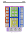

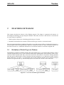
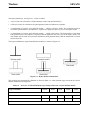
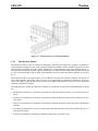
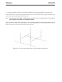
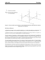
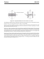
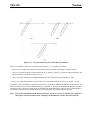
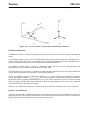
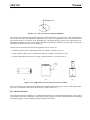
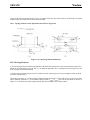
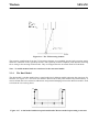
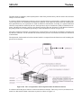
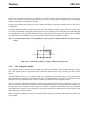

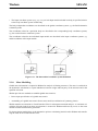
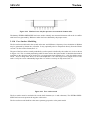
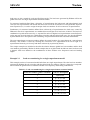
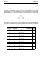

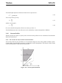
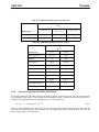
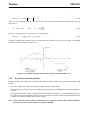

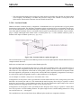


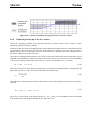

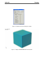
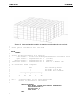
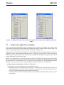


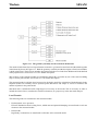
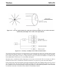
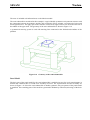

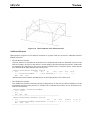
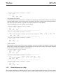


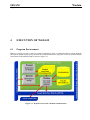
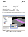

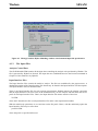


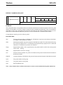
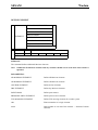


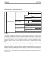


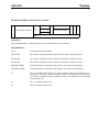


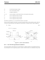
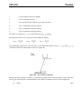
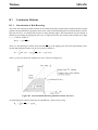


![CURSA [1ex] Catalogue and Table Manipulation](http://vs1.manualzilla.com/store/data/005911996_1-56034bbec42ed74359b0b23f04aae37f-150x150.png)