1
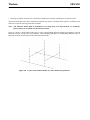
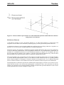
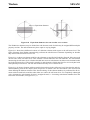
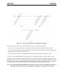
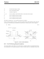
SESAM
Wadam
Program version 8.1
22-JAN-2010
2-47
Linearisation of the problem permits decomposition of the velocity potential φ into the radiation and diffraction components:
φ = φR + φD
φ R = iω
∑
(2.22)
ξj φj
(2.23)
j = 1, 6
φR = φ0 + φ7
(2.24)
The constants ξj denote the complex amplitudes of the body oscillatory motion in its six rigid-body degrees
of freedom and φj the corresponding unit-amplitude radiation potentials. The velocity potential φ7 represents
the disturbance of the incident wave by the body fixed at its undisturbed position. The total diffraction
potential φD denotes the sum of φ7 and the incident wave potential.
On the undisturbed position of the body boundary the radiation and diffraction potentials are subject to the
conditions
φ jn = n j
(2.25)
φ Dn = 0
where (n1, n2, n3) = n and (n4, n5, n6) = r × n, r = (x, y, z). The unit vector n is normal to the body boundary
and points out of the fluid domain. The boundary value problem must be supplemented by a condition of
outgoing waves applied to the velocity potentials φj, j=1,...,7.
2.6.2
Calculation of Wave Loads from Second Order Potential Theory
The second order theory applied in Wadam is described in Ref. /3/ and Ref. /4/. Wadam calculates sum- and
difference-frequency components of the second order forces, moments and rigid body motions (Quadratic
Transfer Functions) in the presence of bi-chromatic and bi-directional waves.
2.6.3
Removal of Irregular Frequencies
Wadam provides an option to remove the irregular frequencies from the radiation-diffraction solution. This
method is based on a modified integral equation obtained by including a panel model of the internal water
plane. The panel model of the water plane is automatically created by Wadam.
2.6.4
Morison’s Equation
Morison’s equation is used in Wadam to calculate contributions to the equation of motion Equation (2.30)
and to calculate the detailed forces F acting on 2D Morison elements and 3D Morison elements. The form of
Morison’s equation used in this calculation is given in Equation (2.26) with the effect of relative motion
included.
2
2
F = ω ( M + ρV M C a )ξ – ω ρV M ( C a + I )x + iωB ( x – ξ ) + f c + f g + f b
Where:
(2.26)


![CURSA [1ex] Catalogue and Table Manipulation](http://vs1.manualzilla.com/store/data/005911996_1-56034bbec42ed74359b0b23f04aae37f-150x150.png)