1
ZAKŁAD SYSTEMÓW ELEKTRONICZNYCH
ATLAS - SOLLICH
ul. Mjr. M. Słabego 2, 80-298 Gdańsk, Poland
tel./fax +48 58 349 66 77
www.atlas-sollich.pl
e-mail: [email protected]
OPERATING MANUAL
ATLAS 0531
ELECTROCHEMICAL UNIT & IMPEDANCE ANALYSER
GDAŃSK 2007
I. INTRODUCTION
ATLAS 0531 ELECTROCHEMICAL UNIT & IMPEDANCE ANALYSER is a precise
five-electrode device which provides measurements of chrono-volt-amperometric characteristics and
impedance spectrums of electrochemical samples.
ATLAS 0531 ELECTROCHEMICAL UNIT & IMPEDANCE ANALYSER is designed as a virtual
machine. This device is a measuring block that is portable and easy to install onto research station
connected via USB interface to a PC computer.
The device has built-in operating software which implements the programming function of the device
and cooperates with AtlasCorr05 PC software installed on a PC computer.
The computer is used both to program the parameters of measurement as well as to register the
results. The PC Computer records the measurement process and visualizes the currently received results.
There is the possibility to disconnect the PC computer after starting the measurement process and receive
the results at the end of this process.
II. THE CONSTRUCTION OF THE DEVICE
ATLAS 0531 EU&IA is made up of:
1. ATLAS 0531 ELECTROCHEMICAL UNIT
-
A five-electrode potentiostat-galvanostat equipped with a linear and step generator
2. ATLAS 0531 IMPEDANCE ANALYSER
-
This analyser provides the measurement of the impedance spectrum within the range of
100KHz to 100uHz
The two devices are built together in one case. It is possible to make this set in two stages.
The first stage is the ATLAS 0531 EU, and the second is the ATLAS 0531 IA, built into the same
case.
The ATLAS 0531 EU&IA is constructed as a compact, reliable, light metal package. It is covered with
solid powder spray which is highly resistant to mechanical effects as well as atmospheric conditions.
The parts necessary for the device are:
-
measurement cable for connection electrochemical cell to the device,
-
replacement test cell – “dummy cell”,
-
temperature sensor,
-
USB cable for communication with PC computer,
-
230 [V] Power cable.
2
III. FUNCTIONS OF THE DEVICE
III.1. Measured parameters
-
The current measurement of working electrode.
-
The potential measurement of working electrode.
-
The potential measurement of reference electrode.
-
The temperature measurement of a cell combined with chrono-volt-amperometric
measurement.
-
Measurement of two external parameters combined with the chrono-volt-amperometric
measurements.
-
The measurement of the impedance spectrum.
III.2. Chrono-volt-amperometric and impedance spectrum measurements
-
The measurement of the retrained potential.
-
The measurement of E(t) and Ipol(t) plots alongside a potentiostatic force.
-
The measurement of E(t) and Ipol(t) plots alongside linear or gradual changes of potential at
selected times of rising, and selected end potential values, combined with 1, 2 or 4 stages of
change.
-
The measurement of E(t) and Ipol(t) plots alongside abrupt changes of potential.
-
The measurement of E(t) and Ipol(t) plots alongside galvanostatic force.
-
The measurement of E(t) and Ipol(t) plots alongside linear or gradual changes of current at
selected times of rising, and selected end current values combined with 1,2 or 4 stages of
change.
-
The measurement of E(t) and Ipol(t) alongside abrupt changes of current.
-
The cyclical measurement of E(t) and Ipol(t) plots alongside the charge/discharge time at
selected current or potential or time values.
-
The measurement of the impedance spectrum:
- for static polarization potential,
- for changes in polarization potential.
-
The possibility of experiment termination after the fulfilment of some additional conditions, e.g.:
- exceeding the voltage or current ranges of a tested object,
- exceeding the voltage ranges of two external devices connected to the measurement
socket of the device,
- exceeding the maximum time of the experiment process.
-
The possibility of cyclical repetition of the experiment.
-
The ossibility of linking different types of experiments in one measurement process.
-
The possibility of visualizing every measured parameter on the plots.
3
-
The possibility of selecting plot axes.
-
The possibility of saving results to a file.
-
The possibility of measurement while in a disconnected PC computer state, and next receive
results after the end of the measurement process or later.
IV. TECHNICAL DATA
-
The maximum voltage of auxiliary electrode CE:
±18 [V]
-
The maximum current of measured electrode:
±1,024 [A]
-
The linear operation range of measured electrode:
±10,240 [V]
-
The maximum current measurement range:
1 [A]
-
The minimum current measurement range:
10 [nA]
-
The resolution of current measurement in range:
16 bits
-
The speed of voltage change in step generator:
1. in ±2[V] range ( step by 62,5[µV]):
1,25 [V/sec]
2. in ±4[V] range ( step by 125[µV]):
2,5 [V/sec]
3. in ±10[V] range ( step by 312,5[µV]):
-
10 [V/sec]
The speed of voltage changes in a linear generator:
1. minimum:
1 [µV/sec]
2. maximum:
100 [V/sec]
-
The maximum speed of voltmeter sampling
-
The frequency range of the impedance measurement:
1. minimum frequency of measurement:
20000 [1/sec]
100 [µHz]
2. maximum frequency of measurement:
-
The maximum amplitude of generator:
-
The impedance range
-
100 [KHz]
1000 [mV]
1. minimum value:
1 [Ω]
2. maximum value:
100[MΩ]
The maximum polarization potential of measured electrode
in impedance measurement time:
±4 [V]
-
The power supply:
230[V] ~ 48-60[Hz]
-
The case dimensions:
168 x 365 x 365 [mm]
4
V. OPERATION OF THE INSTRUMENT
Switch On the power supply by using the main I/O switch which is found on the front panel of the
device. The instrument should be switched for 10 minutes before starting the measurement process.
The following lights on the Atlas 0531 EU&IA should be lit: 1A, POT, OFF, STS1, POWER, OK and PC (if
USB cable is connected to the PC).
Run the AtlasCorr05.exe software according to the details in the chapter titled: SOFTWARE MANUAL.
V.1. Signalling lamps on the front panel:
POWER checklist group:
POWER – The state of being switched on,
OK – Checking of the power circuit inside the device.
STATUS group:
PRG 1 – Is lit when the measurement process has been started,
PRG 2 – Not in use,
BND 3…1 – Determines the type of “Slew Rate” set in binary form:
000 – 10V/µsec,
001 – 1V/µsec,
010 – 100mV/µsec,
011 – 10mV/µsec,
100 – 1mV/µsec,
STS 1 – Blinks while the device is being initialized, and stays lit after correct initialization,
STS 2 – Blinks while reading data from the memory card.
ANALYSER group – Relating to the module’s state for the impedance measurement:
READY – The impedance analyser is ready to work,
TEST – Not in use,
MEAS – The Impedance analyser during the time of measurement,
ERROR – An error occurred during the measurement process.
POTENTIOSTAT MODE group:
POT – Working in the potentiostatic mode,
GLV – Working in the galvanostatic mode,
5
ExD – Not in use,
Rohm – Not in use,
OFE – Not in use,
DUM – Not in use,
Est – The stationary potential measurement state,
WRK – The execution of a measurement experiment.
CURRENT RANGE group:
10uA … 1A – The current range used.
GENERATOR group:
LIN – The linear generator is on,
Up – An increasing slope is generated,
Down – A declining slope edge is generated,
ExtInp – Not in use,.
COM group:
RxD – Receiving data throw the device,
TxD – Transmitting data from the device,
PC – The USB connection to the computer is active.
V.2 Connection of measure cell
Circuit of measure cell connection is viewed on figure (Fig.V.1)
Correct ending of the cable is necessary condition for receiving correct results of the experiment. Correct
connection of cable is viewed in column circuits at the left side of the figure. Incorrect connection of the
cable viewed is in column at the right side of the figure and it is marked with the ring. The incorrect
connection of the cable is able to make obtaining of incorrect results of the measurement.
V.3 Separating of the measuring cell from outside electromagnetic interferences:
External electromagnetic interferences are the significant factor having impact of accuracy
measurement. There are disturbing interferences from 50 [Hz] power supply network, machines, electrical
devices and there are interferences from some kind of radio emitters and of generators. Impact of these
interferences is bigger with it the smaller measuring current value is on measured object. Biggest
impedance of the object means smaller current signal. There is the recognized method of the reduction of
interferences putting the measured object in Faraday's cage. Currently when the mobile phone is common
and present in the environment of the measured object, applying of Faraday's cage is indispensable
(Fig.V.2).
Connection circuit of sample cell is viewed on a figure.
Significant condition of correct use the cage is:
6
1. Connecting the cage to GROUND port of the device by the shortest cable as possible
2. Placement of the measure cell in space of the cage in such a way to minimise capacities
between a cell and sides of the cage (Cc-c name of the capacity on figure). The arrangement
of the cell is resulting in the rise of the large capacity directly on the basis of the cage between
the measuring cell and with the cage. This is able it to cause big measuring errors, especially
at measurements of impedance spectrum. And therefore it is recommending using of the
supports which will tolerate to locate the cell centrally in space of the cage.
7
Fig. V.1 Circuit of cell connection to 0531 device
8
Fig. V.2 Circuit of Faraday’s cage connection to 0531 device
9
VI SOFTWARE MANUAL
VI.1. The installation of drivers
First of all the drivers necessary for the communication of the device via USB should be installed.
The necessary drivers have been attached to the device software.
After connecting the device to the PC computer, the computer should detect the unidentified device,
and it should start the process of installation. The driver files path should be selected during the installation
process. The localization of the drivers is: D:\Drivers\ found on the attached CD.
VI.2. The configuration of PC settings
In order for the device to work properly, it is necessary to set certain properties in the computer
operation system. One need to start the icon labelled System in the Control panel (Fig. VI.1).
Fig. VI.1. PC configuration process
In the system properties click the tap Hardware and click Device manager.
10
New window will appear (Fig. VI.2):
Fig. VI.2. The selection of the configured device
Click USB Serial Port (COM) on the device to selected.
Fig. VI.3. The change of virtual serial port (COM) settings
Under the Port Settings tab the Advanced bar should be chosen. The settings in the new window (Fig
VI.4) should be changed:
Minimum Read Timeout (msec): 100
Minimum Write Timeout (msec): 100
11
Fig. VI.4. The correct values of the bars on the panel
Accept changes by pressing OK.
VI.3. Software installation
The next stage is the software installation for the potentiostat operation. On the attached CD in the
“\install” directory run the setup.exe file. Select the destination directory path while installing the program.
After installation process is complete the new program AtlasCorr05 will appear.
VI.4. Starting the measurement
After double clicking the icon the program starts. On the monitor’s screen a panel appears which
informs you if was communication with the device successful or unsuccessful (Fig. VI.5):
Fig. VI.5. Information about the correctness of transmission
12
After clicking OK the proper program panel appears (Fig. VI.6):
Fig. VI.6. Front program panel
To start the measurement process, a list of experiments and their details should be defined.
Click the Program option on the menu strip and then New program (Fig. VI.7).
Fig. VI.7. The stage of forming the list of experiments
13
A new window then appears (Fig. VI.8):
Fig. VI.8. The program window after clicking on the New program option
The front panel describes the device’s parameters such as the current or voltage ranges and the like. The
details of this panel are described in an other part of this manual. The default settings in most cases are
sufficient for starting the measurement process. Therefore the OK button should be clicked without any
changes of settings. Next, the new experiments have to be added to the list of experiments
(Fig. VI.9):
Fig. VI.9. Process of adding new experiment
In the new panel, the type of the experiment should be selected (Fig. VI.10) e.g.: Potentiodynamic 1 step.
14
Fig. VI.10. Selecting of experiment type
Each type of experiment has been described in another part of this manual. After selecting the
experiment, click the OK button to confirm.
A new panel appears as a result (Fig. VI.11). On this panel, detailed properties of an experiment
should be defined, such as the beginning potential, the end potential, the rate of increase, termination
conditions and many more. More detailed description is in the following chapters.
Fig. VI.11. The edition of experiment details
15
It is necessary to give a filename in order to save(Select File control) the results of an experiment,
the values of potential (Et, E2 potential), the delay between the changing processes of potential (Time t1,
t2), the rising/falling rate (Scan Rate). To observe results on the plots during the measurement time, the
types of plots should be defined. By clicking on Axes X and Axes Y we select the type of data on the X
and Y axes. The Add Plot bar adds the defined plot to the “Types of Plots to View” window showing plots to
view during measurement time. As an example a defined panel is shown below (Fig. VI.12):
Fig. VI.12. An example of an experiment panel filled in
After the details are determined, the settings should be confirmed by pressing OK. In the list of experiments
a new line appears with the type, description and name of the experiment file (Fig. VI.13):
Fig. VI.13. An element of a list of experiments
16
New experiments can be added in a similar way (Fig. VI.14):
Fig. VI.14. Elements of a list of experiments
In order to save all measurement data in one file, the checking box Save all data in one file should be
selected.
In order to start the measurement process, the Run Process bar should be clicked found at the in the left
bottom corner of the panel (Fig. VI.15):
Fig. VI.15. The view of the Run Process bar on the Program panel
A new panel appears on the screen after starting the measurement (Fig. VI.16):
Fig. VI.16. The process of viewing measurement results
17
New values of samples are added to the table during the process. If any plots were added to the
experiment then they will be displayed as well (Fig. VI.17):
Fig. VI.17. The process of plotting the graph
The values of samples are saved onto the file that was defined under the experiment details. The
measurement process can be terminated by pressing the Stop Process bar on the Test Result panel.
VI.5. The experiment details
The user can select from the following types of experiments:
- Cell Disconnect
- Open Circuit
- Potentiostatic
- Potentiodynamic 1 step
- Linear Polarization 2 step
- Potentiodynamic 3 step
- Galvanostatic
- Galvanostatic 2 step
- Galvanodynamic 1 step
- Galvanodynamic 2 step
- Impedance spectrum
18
Cell Disconnect – A delay before starting the experiment.
Open Circuit – A potential measurement on connectors in a free potential state of object.
Potentiostatic – A potential and current measurement by one forcing potential.
Potentiodynamic 1 step – A potential and current measurement by a linear change of forcing potential.
Linear Polarization 2 step – A potential and current measurement by linear change of forcing potential.
The values of potentials are selected in differential ways in relation to the initial value
Potentiodynamic 3 step – A potential and current measurement by linear change of forcing potential. In
this four different values of potential may be defined, which should then be achieved during the experiment.
Galvanostatic – A potential and current measurement during a constant forcing current.
Galvanostatic 2 steps – A potential and current measurement at two defined constant current values.
Galvanostatic 1 step – A potential and current measurement alongside a linear current change.
Galvanostatic 3 step – A potential and current measurement alongside a linear change of current. Four
values of current may be defined which should then be achieved during the experiment.
Impedance spectrum – The impedance spectrum measurement for a given potential.
19
VI.6.1. Cell Disconnect (Fig. VI.18):
Fig. VI.18. Cell Disconnect a panel describing experiment details
Conditions of Termination:
Time – The maximum amount of time for the experiment.
Setup Device:
Default settings – Default settings of the device,
Custom settings – User settings.
Data File:
Select File – Selection of a file in order to save the results of the experiment,
Data Output File – Name of the data file with its directory path.
OK – Accepting the experiment details.
Cancel – Cancelling the defined experiment details.
20
VI.6.2. Open Circuit (Fig. VI.19):
Fig. VI.19. Open Circuit a panel describing the experiment details
Scan Definition:
Initial delay t1 – The amount of time of an experiment.
Conditions of Termination:
Time – The maximum time for the experiment,
Voltage [V] – The minimum and maximum values of potential in the experiment,
Uext1 – The minimum and maximum value of voltage read from an external sensor (for example:
temperature sensor, humidity sensor),
Uext2 – The minimum and maximum value of voltage read from an external sensor (for example:
temperature sensor, humidity sensor).
Type of Data Acquisition (A way of collecting measurement samples):
Fixed Rate – Constant sampling frequency,
Delta – E – Sampling by a selected change of potential,
Delta – I – Sampling by a selected change of current.
21
Graph:
Axes X – The type of data on X axis,
Axes Y – The type of data on Y axis,
Add Plot – Adding a plot type to view during the experiment,
Remove – Removing a plot type from view during the experiment,
Types of plots to view – Plot types visible during the experiment.
Setup Device:
Default settings – Device default settings,
Custom settings – User settings.
Data File:
Select File – The selection of a file in order to save experiment results,
Data Output File – The name of the file with its directory path.
OK – Accepting the experiment details.
Cancel – Cancelling the defined experiment details.
22
VI.6.3. Potentiostatic (Fig. VI.20):
Fig. VI.20. Potentiostatic a panel describing the experiment details
Scan Definition:
Potential E1 [V] – The value of forced potential
Conditions of Termination:
Time – The maximum amount of time for the experiment
Voltage [V] – The minimum and maximum value of potential that may appear in the experiment
Current [A] – The minimum and maximum value of current that may appear in the experiment
Uext1 – The minimum and maximum value of voltage read from an external sensor (for example:
temperature sensor, humidity sensor)
Uext2 – The minimum and maximum value of voltage read from an external sensor (for example:
temperature sensor, humidity sensor)
23
Type of Data Acquisition (A way of collecting measurement samples):
Fixed Rate – The constant frequency of sampling,
Delta – E – Sampling by a selected change of potential,
Delta – I – Sampling by a selected change of current.
Graph: (Plots)
Axes X – The type of data on X axis,
Axes Y – The type of data on Y axis,
Add Plot – Adding a plot type to view during an experiment,
Remove – Removing a plot type from view during an experiment,
Types of plots to view – Plot types visible during an experiment.
Setup Device:
Default settings – Default settings of the device,
Custom settings – User settings.
Data File:
Select File – Selecting a file in order to save results,
Data Output File – The name of the file with its directory path.
OK – Accepting the experiment details.
Cancel – Cancelling the defined details of an experiment.
24
VI.6.5. Potentiodynamic 1 step (Fig. VI.21):
Fig. VI.21. Potentiodynamic 1 step - a panel describing the experiment details
Scan Definition:
Potential E1 [V] – The initial value of potential,
Time t1 – The amount of time for the E1 potential,
Scan Rate (SR1) – The rate of potential increasing/declining,
Potential E2 [V] – The final value of potential,
Time t2 – The amount of time for the E2 potential.
Conditions of Termination:
Time – The maximum amount of time for an experiment,
Voltage [V] – The minimum and maximum value of potential for an experiment,
Current [A] – The minimum and maximum current value for an experiment,
Uext1 – The minimum and maximum value of voltage read from an external sensor (for example:
temperature sensor, humidity sensor),
Uext2 – The minimum and maximum value of voltage read from an external sensor (for example.
temperature sensor, humidity sensor).
25
Type of Data Acquisition (A way of collecting measurement samples):
Fixed Rate – The constant frequency of sampling,
Delta – E – Sampling by a selected change of potential.
Delta – I – Sampling by a selected change of current.
Graph:
Axes X – The type of data on X axis,
Axes Y – The type of data on Y axis,
Add Plot – Adding a plot type to view during an experiment,
Remove – Removing a plot type from viewing during an experiment,
Types of plots to view – Plot types viewed during an experiment.
Setup Device:
Default settings – Default settings of the device,
Custom settings – User settings.
Data File:
Select File – Selecting a file in order to save results,
Data Output File – The name of the file with its directory path.
OK – Accepting the experiment details.
Cancel – Cancelling the defined details of an experiment.
26
VI.6.6. Linear Polarization 2 step (Fig. VI.22):
Fig. VI.22. Linear Polarization 2 steps – a panel describing the experiment details
Scan Definition:
Potential E1 [V] – The initial value of potential –stationary potential is always measured after the
t1 time and before starting the polarization of a sample,
Time t1 – The measurement time of stationary potential E1 - the sample isn’t polarized, only
clamps are connected to the potential measurement,
dE1 [V] – Difference between initial value of potential E1 in relation to its minimum value in the
cycle,
Scan Rate (SR1) – The rate of increasing/declining dE1 potential,
dE2 [V] – The difference between the maximum value of potential in the cycle in relation to its
initial value E1,
Scan Rate (SR2) – The rate of increasing/declining dE2 potential,
No. of Cycles – Number of repetitions in a defined sequence.
Conditions of Termination:
Time – The maximum amount of time for an experiment,
27
Voltage [V] – The minimum and maximum value of potential for an experiment,
Current [A] – The minimum and maximum current value for an experiment,
Ipol [A] – The minimum and maximum value of current that can appear in an experiment,
Uext1 – The minimum and maximum value of voltage read from an external sensor (for example:
temperature sensor, humidity sensor),
Uext2 – The minimum and maximum value of voltage read from an external sensor (for example:
temperature sensor, humidity sensor).
Type of Data Acquisition (A way of collecting measurement samples):
Fixed Rate – The constant frequency of sampling,
Delta – E – Sampling by a selected change of potential,
Delta – I – Sampling by a selected change of current.
Graph:
Axes X – The type of data on X axis,
Axes Y – The type of data on Y axis,
Add Plot – Adding a plot type to view during a time of measurement,
Remove – Removing a plot type from viewing during an experiment,
Types of plots to view – Plot types viewed during an experiment.
Setup Device:
Default settings – Default settings of the device,
Custom settings – User settings.
Data File:
Select File – Selecting a file in order to save results,
Data Output File – The name of the file with its directory path.
OK – Accepting the experiment details.
Cancel – Cancelling the defined details of an experiment.
28
VI.6.7. Potentiodynamic 3 steps (Fig. VI.23):
Fig. VI.23. Potentiodynamic 3 steps – a panel describing experiment details
Scan Definition:
Potential E1 [V] – The initial value of potential,
Time t1 – The amount of time of E1 potential,
Scan Rate(SR1) – The rate of increasing/declining potential,
Potential E2 [V] – The value of E2 potential,
Time t2 – The amount of time of E2 potential,
Use – Switching on the Use will allow the following steps, 3 and 4, to be performed,
Scan Rate (SR2) – The rate of increasing/declining potential,
Potential E3 [V] – The value of E3 potential,
Time t3 – The amount of time of E3 potential,
Use – Switching on the Use option allows step 4 to be performed,
Scan Rate (SR3) – The rate of increasing/declining potential,
Potential E4 [V] – The value of E4 potential,
Time t4 – The amount of time of E4 potential,
No. of Cycles – The number of repetitions in a defined sequence.
29
Conditions of Termination:
Time – The maximum amount of time for an experiment,
Voltage [V] – The minimum and maximum value of potential for an experiment,
Current [A] – The minimum and maximum current value for an experiment,
Uext1 – The minimum and maximum value of voltage read from an external sensor (for example:
temperature sensor, humidity sensor),
Uext2 – The minimum and maximum value of voltage read from an external sensor (for example:
temperature sensor, humidity sensor)
Type of Data Acquisition (A way of collecting measurement samples):
Fixed Rate – the constant frequency of sampling,
Delta – E – Sampling by a selected change of potential,
Delta – I – Sampling by a selected change of current.
Graph:
Axes X – The type of data on X axis,
Axes Y – The type of data on Y axis,
Add Plot – Adding a plot type to view during an experiment,
Remove – Removing a plot type from viewing during an experiment,
Types of plots to view – Plot types viewed during an experiment.
Setup Device:
Default settings – Default settings of the device,
Custom settings – User settings.
Data File:
Select File – Selecting a file in order to save results,
Data Output File – The name of the file with its directory path.
OK – Accepting the experiment details.
Cancel – Cancelling the defined details of an experiment.
30
VI.6.8. Galvanostatic (Fig. VI.24):
Fig. VI.24. Galvanostatic – a panel describing the experiment details
Scan Definition:
Ipol1 [A] – The value of a forced current.
Conditions of Termination:
Time – The maximum amount of time for an experiment,
Voltage [V] – The minimum and maximum value of potential for an experiment,
Current [A] – The minimum and maximum current value for an experiment,
Uext1 – The minimum and maximum value of voltage read from an external sensor (for example:
temperature sensor, humidity sensor),
Uext2 – The minimum and maximum value of voltage read from an external sensor (for example:
temperature sensor, humidity sensor).
31
Type of Data Acquisition (A way of collecting measurement samples):
Fixed Rate – The constant frequency of sampling,
Delta – E – Sampling by a selected change of potential,
Delta – I – Sampling by a selected change of current.
Graph:
Axes X – The type of data on X axis,
Axes Y – The type of data on Y axis,
Add Plot – Adding a of plot type to view during an experiment,
Remove – Removing a plot type from viewing during an experiment,
Types of plots to view – Plot types viewed during an experiment.
Setup Device:
Default settings – Default settings of the device,
Custom settings – User settings.
Data File:
Select File – Selecting a file in order to save results,
Data Output File – The name of the file with its directory path.
OK – Accepting the experiment details.
Cancel – Cancelling the defined details of an experiment.
32
VI.6.9. Galvanostatic 2 steps (Fig. VI.24B):
Fig. VI.24B. Galvanostatic 2 steps – a panel describing the experiment details
Scan Definition:
t1 – The time from the beginning of the experiment to the achieving of the forced current value I1.
If that time is shorter than 5 seconds then the polarization current value is set at 0,00[A] and a CE
electrode is connected to the object. If the time is longer than 5 seconds then the current value is
set at 0,00[A] and the CE electrode is disconnected from the object.
I1 [A] – The value of a forced current.
t2-max – The maximum amount of time for the I1 current value.
Ew1off[V] – The value of Ew potential in which the termination of forcing current I1 happens.
End for:
Ew>Ew1off – The I1 forcing is terminated if the Ew voltage reaches a grater value
than the Ew1offvoltage,
Ew<Ew1off – The I1 forcing is terminated if the Ew voltage reaches a lower value
than theEw1off voltage.
t3 – The delay time between the end of I1 forcing and the beginning of I2 forcing. If this time is
shorter than 5 seconds then the polarization current value is set at 0,00[A] and the CE
electrode is not disconnected from the object. If the delay time is longer than 5 seconds
then the polarization current value is set at 0,00[A] and the CE electrode is disconnected
33
from the object.
I2 [A] – The value of a forced current.
t4-max – The maximum amount of time of forcing by a current with a value of I2.
Ew2off[V] – The value of Ew potential at which the termination of the I2 current forcing happens.
End for: Ew>Ew2off – the I2 forcing is terminated if the Ew voltage exceeds the Ew2off value
Ew<Ew2off – the I2 forcing is terminated if the Ew voltage is less than the Ew2off
value.
Use – Activation of the termination condition after exceeding a specified Ew value.
No. of Cycles – The number of repetitions in a defined sequence.
Conditions of Termination:
Time – The maximum amount of time for an experiment,
Voltage [V] – The minimum and maximum value of potential for an experiment,
Current [A] – The minimum and maximum current value for an experiment,
Uext1 – The minimum and maximum value of voltage read from an external sensor (for example:
temperature sensor, humidity sensor),
Uext2 – The minimum and maximum value of voltage read from an external sensor (for example:
temperature sensor, humidity sensor).
Type of Data Acquisition (A way of collecting measurement samples):
Fixed Rate – The constant frequency of sampling,
Delta – E – Sampling by a selected change of potential,
Delta – I – Sampling by a selected change of current,
Graph:
Axes X – The type of data on X axis,
Axes Y – The type of data on Y axis,
Add Plot – Adding a plot type to view during an experiment,
Remove – Removing a plot type from viewing during an experiment,
Types of plots to view – plot types viewed during an experiment.
Setup Device:
Default settings – Default settings of the device,
Custom settings – User settings.
Data File:
Select File – Selecting a file in order to save results,
Data Output File – The name of the file with its directory path.
OK – Accepting the experiment details
Cancel – Cancelling the defined details of an experiment
34
VI.6.10. Galvanodynamic 1 step (Fig. VI.25):
Fig. VI.25. Galvanodynamic 1 step a panel describing the experiment details
Scan Definition:
Ipol1 [A] – The initial current value,
Time t1 – The amount of time of the I1 current,
Scan Rate (SR1) – The rate of current increase/decrease,
Ipol2 [A] – The final value of the current,
Time t2 – The amount of time of the I2 current.
Conditions of Termination:
Time – The maximum amount of time for an experiment,
Voltage [V] – The minimum and maximum value of potential for an experiment,
Current [A] – The minimum and maximum value of current for an experiment,
Ipol [A] – The minimum and maximum value of current that can appear in an experiment
Uext1 – The minimum and maximum value of voltage read from an external sensor (for example:
temperature sensor, humidity sensor),
Uext2 – The minimum and maximum value of voltage read from an external sensor (for example:
temperature sensor, humidity sensor).
35
Type of Data Acquisition (A way of collecting measurement samples):
Fixed Rate – The constant frequency of sampling,
Delta – E – Sampling by a selected change of potential,
Delta – I – Sampling by a selected change of current.
Graph:
Axes X – The type of data on X axis,
Axes Y – The type of data on Y axis,
Add Plot – Adding a plot type to view during an experiment,
Remove – Removing a plot type from viewing during an experiment,
Types of plots to view – The plot types viewed during an experiment.
Setup Device:
Default settings – Default settings of the device,
Custom settings – User settings.
Data File:
Select File – Selecting a file in order to save results,
Data Output File – The name of the file with its directory path.
OK – Accepting the experiment details.
Cancel – Cancelling the defined details of an experiment.
36
VI.6.11. Galvanodynamic 3 steps (Fig. VI.26):
Fig. VI.26. Galvanodynamic 3 steps. A panel describing the experiment details
Scan Definition:
Ipol1 [A] – The initial value of current,
Time t1 – The amount of time of the I1 current,
Scan Rate (SR1) – The rate of increasing/declining current,
Ipol2 [A] – The value of the I2 current,
Time t2 – The amount of time of the I2 current,
Scan Rate (SR2) – The increasing/decreasing rate of the current,
Ipol3 [A] – The value of the I3 current,
Time t3 – The amount of time of the I3 current,
Scan Rate (SR3) – The rate of increasing/decreasing current,
Ipol4 [A] – The value of the I4 current,
Time t4 – The amount of time of the I4 current,
No. of Cycles – The number of repetitions in a defined sequence.
37
Conditions of Termination:
Time – The maximum amount of time for an experiment,
Voltage [V] – The minimum and maximum value of potential for an experiment,
Current [A] – The minimum and maximum value of current for an experiment,
Uext1 – The minimum and maximum value of voltage read from an external sensor (for example:
temperature sensor, humidity sensor),
Uext2 – The minimum and maximum value of voltage read from an external sensor (for example:
temperature sensor, humidity sensor).
Type of Data Acquisition (A way of collecting measurement samples):
Fixed Rate – The constant frequency of sampling,
Delta – E – Sampling by a selected change of potential,
Delta – I – Sampling by a selected change of current.
Graph:
Axes X – The type of data on X axis,
Axes Y – The type of data on Y axis,
Add Plot – Adding a plot type to view during an experiment,
Remove – Removing of plot type from viewing during an experiment.
Types of plots to view – The plot types viewed during an experiment.
Setup Device:
Default settings – Default settings of the device,
Custom settings – User settings.
Data File:
Select File – Selecting a file in order to save results,
Data Output File – The name of the file with its directory path.
OK – Accepting the experiment details.
Cancel – Cancelling the defined details of the experiment.
38
VI.6.12. Impedance spectrum (Fig. VI.27):
Fig. VI.27. Impedance sweep frequency. A panel describing the experiment details
Scan Definition:
Potential E1 [V] – The potential offset,
Time t1 – The delay in starting the potential,
AC Amplitude [mV] – The amplitude of measurement signal,
Initial Frequency [Hz],
Final Frequency 1 [Hz] – The final frequency of the first interval,
Final Frequency 2 [Hz] – The final frequency of the second interval,
Final Frequency 3 [Hz] – The final frequency of the third interval,
Final Frequency 4 [Hz] – The final frequency of the fourth interval.
Points/dek: - The number of points for a decade in a specified frequency interval.
Type of Scale: – Selecting frequency in a logarithmic or decade scale.
Use – Switch on/off a specified frequency interval.
39
Conditions of Termination:
Time – The maximum amount of time for an experiment,
Voltage [V] – The minimum and maximum value of potential for an experiment,
Current [A] – The minimum and maximum value of current for an experiment,
Uext1 – The minimum and maximum value of voltage read from an external sensor (for example:
temperature sensor, humidity sensor),
Uext2 – The minimum and maximum value of voltage read from an external sensor (for example:
temperature sensor, humidity sensor).
Type of Data Acquisition (A way of collecting measurement samples):
Fixed Rate – The constant frequency of sampling,
Delta – E – Sampling by a selected change of potential,
Delta – I – Sampling by a selected change of current.
Graph:
Axes X – The type of data on X axis,
Axes Y – The type of data on Y axis,
Add Plot – Adding a plot type to view during an experiment,
Remove – Removing a plot type from viewing during an experiment.
Types of plots to view – The plot types viewed during an experiment.
Setup Device:
Default settings – Default settings of the device,
Custom settings – User settings.
Data File:
Select File – Selecting a file in order to save results,
Data Output File – The name of the file with its directory path.
OK – Accepting the experiment details.
Cancel – Cancelling the defined details of an experiment.
40
VI.7. The device setup (Fig. VI.30):
The details of the device setup that it will work with, should be defined when the experiment
parameters are determined. The device options panel appears after selecting Program->New Program
from the menu. (Fig. VI.27).
Fig. VI.28. One of the ways of selecting the panel with device options
After selecting this element the panel with so called, global options appears. The global option panel
settings will be used if in the options of any experiment the Default Settings options will be chosen. Global
settings also can later be changed by selecting the Options->Pstat/Gstat setup in an another panel as
well. (Fig. VI.29):
Fig. VI.29. The method of selecting a panel with device options
As a result of this operation a new panel opens (Fig. VI.30)
Current range – The range between the minimum and maximum current value.
Potential range – The range between the minimum and maximum voltage value.
Pstat – The maximum increasing speed of the generator signal.
I – Turning on/off the current measurement.
Ew – Turning on/off the Ew voltage measurement.
Ece – Turning on/off the Ece voltage measurement.
Tmp – Turning on/off the Tmp voltage measurement.
Uext – Turning on/off the Uext1 voltage measurement.
Uext2 – Turning on/off the Uext2 voltage measurement.
Slew Rate – The degree of smoothing out the steps in a digital generator (Fig. VI.31, VI.32).
Sweep Generator – A linear/digital type of generator (Fig. VI.31, VI.32, VI.33).
41
Fig. VI.30. A panel with definitions of device options
Fig. VI.31. An example of a signal from a digital generator (Slew Rate: 10[V/µsec])
42
Fig. VI.32. An example of a signal from a digital generator (Slew Rate: 1[mV/µs])
Fig. VI.33. An example of a signal from a linear generator
43
Controls:
Save as default – Save the actual parameters and use them in the next running of the program.
OK – Accept changes.
Cancel – Cancel changes.
VI.8. Plots
The results of measurements can be viewed on plots. The types of plots should be defined in the
details of the experiments (VI.IV.). Panels of defined plots will appear on the screen after starting the
measurement process (Fig. VI.34). A blue mark can be used to enable the observance of measurement
value points very precisely. The Yellow and pink lines are used to select areas of the plot that can be
enlarged for precise observation.
Fig. VI.34. An example panel of a plot
Y Log Scale , X Log Scale – Selecting a scale (logarithmic/decimal).
Y Grid, X Grid – Displaying a grid on the plot or not displaying a grid
Zoom Plot – Enlarging a part of the plot. The enlarged area is selected by a line (yellow and pink) formed
on the plot
Default View – An overall view of the measurement.
Print – Printing the plot.
X-coordinate, Y-coordinate – Coordinates of the blue mark.
Exit – Closing the plot.
44
VI.9. Receiving data from the internal memory of the device
All data can be read from the internal memory after the measurement has been made. This is
especially significant in a situation when the computer was switched off during the time of the
measurement. After the end of measurement it is possible to read these data at a time that is convenient
for the user. In order to do this use the Get flash data option from the Program menu
(Fig. VI.35):
Fig. VI.35. The reading data from the device memory
A filename should be selected in the next panel to record data for first executed experiment.
The „_X” element will be added to the end of a filename for the following experiments. The „X”
element is the number of the experiment (Fig. VI.36):
Fig. VI.36. Selecting the file to record data
45
After the file has been selected the process of receiving the data from the device and saving the data
on the PC computer begins (Fig. VI.37):
Fig. VI.37. The process of receiving data from the device
VI.10.The conversion of impedance results to a compatible format with the analysis application program „gl_ident”
The program enables the conversion of impedance measurement results format to be compatible
with the impedance objects analyse program: gl_ident.exe (Fig. VI.38):
Fig. VI.38.The impedance results conversion process
46
Fig. VI.39.The file conversion panel
Select – Selecting the file to be converted.
Export – Running the conversion process of the file.
Exit – Closing the panel.
VI.11. The conversion of impedance results to a format compatible with the analysis application –
program “Boukamp”
This program enables the conversion of impedance measurement results to a format that is
compatible with the impedance objects analysis program: impedance data table. This impedance table
consists of three columns. One is frequency, the second one is ReZ and the last is ImZ (Fig. VI.40):
Fig. VI.40.The impedance results conversion process
Fig. VI.41.The file conversion panel
Select – Selecting the file to be converted.
Export – Running the conversion process of the file
Exit – Closing the panel.
47
VI.12. Reseting the device
If for of any reason it happens that a program is started while the device is busy e.g. with
measurement, in order to start a new measurement process it is necessary to reset the device first (Fig.
VI.42):
Fig. VI.42. Resetting the device
48