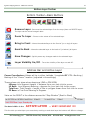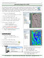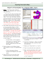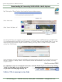
Download 2015 ADMS User Manual

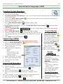
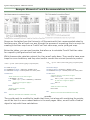
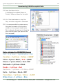
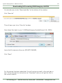
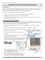
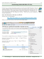
Ag Data Mapping Solu on - ADMS User Manual
1
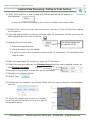
“The”
Ag
Data
Mapping
Solution
Soil Sampling
Fertilizing
Seeding
Drainage
2015 User Manual
GK Technology, Inc. - 204 Fi h Street East, Halstad, MN - 855-458-3244 - www.gktechinc.com
Ag Data Mapping Solu on - ADMS User Manual
3
Contents
File Storage & Structure Layout ....................................................................................... 8
Getting Started with Ag Data Mapping Solution .......................................................... 9
Settings ................................................................................................................. 10-17
Window Dock Settings ....................................................................................... 18-20
Toolbars
Top Toolbar—Map Toolbar .................................................................................. 21-22
Bottom Toolbar—Drawings / Surfaces /Web Layers/ Multi-Band Images ................. 23-28
Drawing Tools (Polygons, Lines & Points) ......................................................................... 29
Extracting Drawing Layers from a Mass Collection ................................................. 30-32
Hand Drawing—Boundaries .................................................................................... 33
Merging Boundaries (Poly-Polygons) ........................................................................ 34
Hand Drawing—Lines & Points ................................................................................ 35
Hand Drawing—Multi-Points .................................................................................... 36
Collect with GPS Using Ag Data Mapping Solution (Map Window) ................................. 37
Decomposing a Poly-Polygon ................................................................................... 38
Moving Vertices & Moving Points ............................................................................. 39
MY NOTES ............................................................................................................. 40-41
Quick Notes for Satellite Imagery ................................................................................... 42
Creating Zones from Imagery
Creating Grower, Farm, Field................................................................................... 43
Creating Boundaries ............................................................................................... 44
Draw a Field Boundary .................................................................................. 45
Save Boundary from a CLU ............................................................................ 46
Creating Boundary From Mass Collection .................................................... 47-48
Extract TIFF Image From NAIP ................................................................................ 49
Extract Images From Web Layers ....................................................................... 50-55
Creating Guide Lines for Image Extraction ................................................................ 56
Automated Zone Creation .................................................................................. 57-58
Manual Image Extraction ................................................................................... 59-61
Inverting Image Values .......................................................................................... 62
Correlation Matrix ............................................................................................. 63-64
Merging Images (Avg of All Layers) ......................................................................... 65
Coloring and Prepping - Surfaces ........................................................................ 66-67
Manual Zone Creation ....................................................................................... 68-69
Thematic Raster Settings ........................................................................................ 70
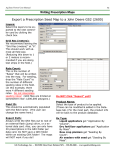
Creating Nutrient Layers—(Prescriptions)
Creating Fertilizer Products .................................................................................... 71
Creating Prescription Maps ..................................................................................... 72
GK Technology, Inc. - 204 Fi h Street East, Halstad, MN - 855-458-3244 - www.gktechinc.com
Ag Data Mapping Solu on - ADMS User Manual
4
Contents
Creating Prescription Maps—Manually....................................................................... 73
Common Name Mapping Database ........................................................................... 74
Color Layers By Theme ...................................................................................... 75-79
Creating Nutrient Layers - Manually ......................................................................... 80
Creating Prescription Maps - Manually ...................................................................... 81
Using CSV - XLS Soil Test Results ....................................................................... 82-86
Using CSV - XLS Soil Test Results Phosphorous Conversion ........................... 83-84
Using Blend Groups ................................................................................................ 87
Enforcing Min and Max Rates ................................................................................... 88
Creating a ModArea or Check Strip & Editing Raster Values ................................... 89-90
Creating Yield Goal Map—Adjusting Range ........................................................... 91-93
Creating Yield Goal Map—Assigning New Values ................................................... 93-94
MY NOTES .................................................................................................................. 95
Quick Notes for Grid Sampling........................................................................................ 96
Grid Sampling
Setting up a Grid ........................................................................................... 97-100
Labeling Grid Points ............................................................................................ 101
Moving Grid Points .............................................................................................. 102
Creating Custom Grid Points ......................................................................... 103-107
Creating Nutrient Layers ............................................................................... 108-114
Creating Nutrient Layers Phosphorous Conversion ................................... 110-111
Common Name Mapping .............................................................................. 113
Printing Grid Nutrient Layers ......................................................................... 115-117
Using Scripts to Write Prescriptions ................................................................ 118-120
Sampling Methods ....................................................................................... 121-122
MY NOTES ................................................................................................................ 123
Making a Test Prescription .................................................................................... 124-126
Exporting Prescription Maps
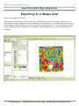
Shape Grid—Export Overview… ............................................................................. 127
Shape Grid—Supported Controllers… ............................................................... 128-132
Shape Contours—Export Process ........................................................................... 133
FODM Device—Export Overview ...................................................................... 134-136
FODM Device—Supported Controllers .............................................................. 137-142
Topcon X20 / Zynx ....................................................................................... 143-144
John Deere GRX—2600 & 2630 Controller ............................................................... 145
MY NOTES ................................................................................................................ 146
Printing (Batch / Multi / Bitmap) ........................................................................... 147-150
Exporting Files as KMZ for Google Earth™ .............................................................. 151-152
Exporting Files as KML for Google Earth™ .............................................................. 153-154
GK Technology, Inc. - 204 Fi h Street East, Halstad, MN - 855-458-3244 - www.gktechinc.com
Ag Data Mapping Solu on - ADMS User Manual
5
Contents
Quick Notes for Topography RTK .................................................................................. 155
Quick Notes for Topography LIDAR ............................................................................... 156
Creating Topography & Watersheds .............................................................................. 157
Importing Data .................................................................................................... 158
Adjusting Levels between Multiple “Point” .shp Files ................................................. 159
Merge .shp files with Z Adjust ........................................................................ 160-161
Merge All Visible .shp files ..................................................................................... 162
Cleaning Elevation SHP - Database ....................................................................... 163
Creating the Topography Map................................................................................ 164
Grid the Points ........................................................................................... 165
Select the Boundary .................................................................................... 166
Cropping the Grid to a Boundary .................................................................. 167
Processing LIDAR LAS Files ............................................................................ 168-171
Registering LAZ Extractor ............................................................................ 169
Running the Watershed Modeling Routine ............................................................... 172
Apply the Point Offset.................................................................................... 173-175
Re-Project the Raster ........................................................................................... 176
LiDAR-RTK Merge ........................................................................................ 177-181
MY NOTES ................................................................................................................ 182
Quick Notes for Drainage Planning ......................................................................... 183-184
Creating Tile Plans
Overview of Tile Planning and Project.. ............................................................ 185-186
Creating Outlet Points .......................................................................................... 187
Adjusting Elevation With Mod Area ......................................................................... 188
Merge Topography.grd files ................................................................................... 189
Creating Tile Plan - Setbacks (Buffer Select Items) .................................................. 190
Designing Mains .................................................................................................. 191
Adding Main Depth Points .............................................................................. 192-193
Pattern Design & Guide Lines ................................................................................ 194
Calculating Tile Size ............................................................................................. 195
Drawing Tile Plan ................................................................................................. 196
Exporting Tile Plan to AGPS Pipe Pro .............................................................. 197-200
Processing Yield Data
Processing through Yield Editor....................................................................... 201-204
Processing KB / GK Yield Data ........................................................................ 205-210
Cleaning Yield In ADMS ................................................................................. 209-211
Normalizing & Merging Yield ........................................................................... 212-213
Yield—Create Grid From Polygon ............................................................................ 214
Yield—Create Grid From Points .............................................................................. 215
Yield to layer merge Script for holes ....................................................................... 216
Processing Yield Data to Net Profit Map .................................................................. 217
GK Technology, Inc. - 204 Fi h Street East, Halstad, MN - 855-458-3244 - www.gktechinc.com
Ag Data Mapping Solu on - ADMS User Manual
6
Contents
Processing Veris Data
Importing & Surfacing Veris DAT Files .............................................................. 218-219
Query Tools ......................................................................................................... 220-221
Summarize Another Layer ..................................................................................... 222-224
Advanced Scripting
Getting Started with Map Math .............................................................................. 225
What is a Null Value? & Declaring and Using Variables ...................................... 226-227
Introduction to Functions, Object, Enumerations and Collections ......................... 228-229
Raster Object and the Rasters Collection ................................................................ 230
Example: Minnesota P & K Recommendation for Corn .............................................. 231
Opening a Script Editor in Excel 2007 & 2003 ................................................... 232-233
P & K Continued—Introducing—Select Case ...................................................... 234-235
Script Functions, Using Functions, Map Math Controls ...................................... 236-2237
System.Math Functions ........................................................................................ 238
Using GK Created Scripts................................................................................ 239-242
Quick Notes for GPS
In Field General .................................................................................................... 243
In Field Quick Mark Points ...................................................................................... 244
In Field Lines & Boundaries .................................................................................... 245
Setup Instructions ................................................................................................. 246
GK—VR Control Quick Start Guide .......................................................................... 247-248
Run ADMS as Administrator ......................................................................................... 249
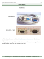
Veris Logging
Hardware Setup .................................................................................................. 250
Cables................................................................................................................ 251
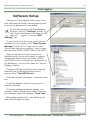
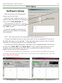
Software Setup ............................................................................................. 252-253
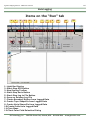
“Run” Tab Items .................................................................................................. 254
Downloading USDA Geospatial Data........................................................................ 255-259
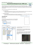
Setting Up Web Based Background Layers (WMS) .................................................... 260-262
Downloading and Processing USGS Imagery (GLOVIS)
Downloading Imagery .................................................................................... 263-268
Landsat Data Processing....................................................................................... 269
Landsat Data Processing - Merging Images ............................................................. 270
Landsat Data Processing - Cutting Images by Shape File .................................... 271-273
Landsat Data Processing - Cutting to Trade Territory ......................................... 274-275
Using Satshot Website for Downloading Imagery ...................................................... 276-279
GK Technology, Inc. - 204 Fi h Street East, Halstad, MN - 855-458-3244 - www.gktechinc.com
Ag Data Mapping Solu on - ADMS User Manual
7
Contents
Downloading LIDAR Data
International Water Institute ........................................................................... 280-281
ND LIDAR Dissemination ................................................................................ 282-284
ND LIDAR Dissemination Using FileZilla ................................................... 285-286
Minnesota DNR FTP Download ......................................................................... 287-289
Iowa LIDAR Data ........................................................................................... 290-291
Downloading & Processing USGS LIDAR - Earth Explorer ........................................... 292-295
LIDAR—LAS Catalog Creation (LAS & LAZ) .................................................................... 296
MY NOTES ................................................................................................................ 297
Glossary
GIS Terms ................................................................................................... 298-301
GK Technology, Inc. - 204 Fi h Street East, Halstad, MN - 855-458-3244 - www.gktechinc.com
Ag Data Mapping Solu on - ADMS User Manual
8
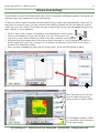
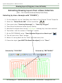
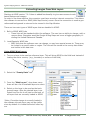
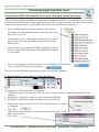
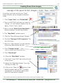
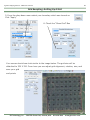
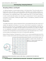
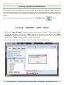
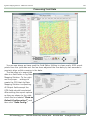
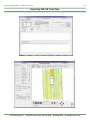
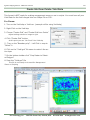
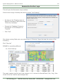
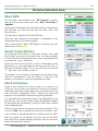
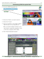
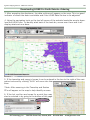
File Storage & Structure Layout
When you open up ADMS you will find that
every window has Grower-Farm-Field as drop
downs in the upper left corner. This is how to
select the field and files to be used. Also, the
names located in these drop downs are going
to print on the side of most of the maps. Ag
Data Mapping Solution software is based on a
very simple folder file format. When you go to
Windows Explorer to look at your files and
folders, the names displayed on the folders in
the “GKData” folder are the same seen in Ag
Data Mapping Solution. You can name, rename
and create folders in either ADMS or Windows
Explorer (you may get errors in both windows
if you have files open in the folders you are renaming).
Below is an example of how to build the file
structure. If you are a farm with only one (1)
entity, then use this structure: (ex. Grower“Johnson Bros Inc” & “Farm-Johnson Bros Inc”
then your Fields). Take note of Field “Sec 32
NE Qtr”; it is populated with folders of years.
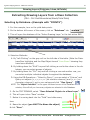
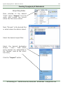
At the end of each year, place all your data into a completed year folder. Using some sort of
Ag Data Mapping Solution
file structure similar to the “2004” example
(Application, Imagery, Yield and Topography
folders). If “Topography” data is only collected every few years, you may want to move
that up one level to be stored in the “Field”
folder. Only create folders for information
that is there, having an empty “Topography”
folder stored in a “Year” folder can be confusing. It may make you think data was collected that year when it really was NOT. If the
field is farmed as one field year-in and yearout, the “Boundary” file should stay in the
“Field” folder. If the field is farmed differently
every year, then the “Boundary” should be
stored in the “Year” folder. As each project is
finished throughout the year, go ahead and
create a folder, ex. “Application Maps”. Then
at the end of the year, create a “2007” folder
and move the “Application”, “Yield” and
“Topography” folders into the “Year” folder.
This will make for quicker and more efficient
use of ADMS. It also makes it easier to know
where all the files are from year to year.
Windows Explorer
GK Technology, Inc. - 204 Fi h Street East, Halstad, MN - 855-458-3244 - www.gktechinc.com
Ag Data Mapping Solu on - ADMS User Manual
9
Getting Started With Ag Data Mapping Solution
To get started with Ag Data Mapping Solution, you need to have some base data in place to
work with. You will need some “Properly” geo-referenced piece of data. Meaning that the
data sets are in either Latitude / Longitude or UTM projections system using WGS84 or
NAD83.
TO GET STARTED YOU NEED AT LEAST 1 OF THESE ITEMS
County Data set for the area you are working (County Data—tab)
NAIP images (USDA-Geospatial)
DRG images (USDA-Geospatial)
Soils Maps (USDA-Geospatial)
Townships & Sections Maps (USDA-Geospatial)
Roads, Railroads & Water ways (TIGER Data)
Data Set to build Maps—need one or more of these (more is usually better)
Satellite / Aerial Imagery (Imagery—tab)
Images USGS
Images UMAC
Topography from LIDAR
Other Imagery sources
NAIP Images (County Data—tab)
Yield data (Raw Data card or .shp files) (Field Data—tab)
Veris data (Raw Data card or .shp files) (Field Data—tab)
Topography from RTK (Raw Data card or .shp files) (Field Data—tab)
Below is a “Rough Outline” of the Process to use this data in the field.
Build - Client / Farm / Field structure in ADMS
Draw <> Collect <> Extract <> Import - Field Boundary
For VRT Mapping
Create Management Zones or Sample
Grids
For Topography Mapping
Import & Process topography data
Inspect topography accuracy / outlets
Soil Sample
Process watersheds / contours
Set application rates
Create surface / tile drainage plan
Enter application values (create prescriptions)
Create background data sets for controller or infield display
Write prescription to controller
Print “Hard copy” map with total LBS of
product
Print “Hard copy” map for taking notes &
taking to the field
GK Technology, Inc. - 204 Fi h Street East, Halstad, MN - 855-458-3244 - www.gktechinc.com
Ag Data Mapping Solu on - ADMS User Manual
10
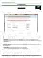
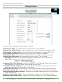
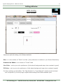
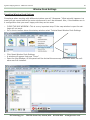
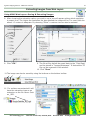
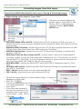
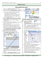
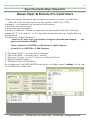
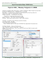
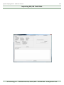
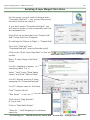
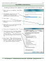
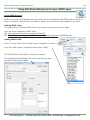
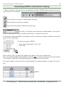
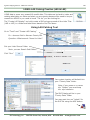
Settings Window
Data Storage
These next pages will walk you through the base settings for ADMS.
Use the “Browse” button to set the location where the software will look for the different data sets.
Software DEFAULTS are shown above.
Root Data = Grower / Farm / Field data sets and the location of many operating files (color tables, templates, blend groups, scripts and base operating database).
County Data = Location where you store data relative to your County or Region. This data may be
roads, sections, townships, soils or county wide images (NAIP). Mostly data downloaded from USDA GeoSpatial website.
Imagery Data = Location where you store satellite imagery scenes and wide area topography data.
Pocket PC Data Folder = Location where you would have folders for GK Pocket Field Recs or Pocket VR
mobile platforms.
Operator Name = users name used for tracking processed data.
NOTE: The name and spaces must be less that 12 characters long.
The beauty of ADMS is the ability to run and utilize data sets off of USB devices and your Local disk drives.
Example would be leaving all you Root Data (grower data) on the “C:” drive and running all your County Data off a USB device “D:” or a “Mapped Network Drive”
NOTE: Read / Write speeds may be GREATLY reduced depending on the speed of your device.
GK Technology, Inc. - 204 Fi h Street East, Halstad, MN - 855-458-3244 - www.gktechinc.com
Ag Data Mapping Solu on - ADMS User Manual
11
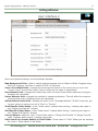
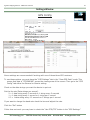
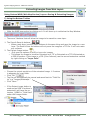
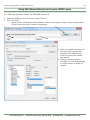
Settings Window
User Interface
Above are optional settings, not the software defaults.
Default Color Table—color table used for most functions in the software.
Default Color Table (Zones) - color table used only in Auto Zone & Extract Image to Zone
Default Units for New Layers—Units that will be used as default in creating “GRD” files
Process PFR_LOG Files as—Method by which “App Log” GPS data is collected
Default Point Style—Is the shape of “Data Points” (circle / square / triangle/cross-hair)
Default Point Scale Mode—the explanation below will using “5” as the value
Pixel Scale—zooming in and out on a data point it would always be 5 “PIXELS” wide
World Scale—data points would be “5” “Feet” wide
Zoom in = points getting larger
Zoom out = points getting smaller
Boundary Effect Filter Distance—how many “METERS” in the “Boundary Effect Filter reaches.
Only applies to use in Auto Zone & Extract Image to Zone tools
Print Map to Bitmap Multiplier—1 = 1to1 ratio to the pixels on the PC display screen. 2 will
double the resolution making the files 4 times larger.
Default Pixel Point Size—set the points to “Pixel” size attached to Default Point Scale Mode
Default World Point Size— set the points to “Foot” size attached to Default Point Scale Mode
Default Image Resolution (Meters) - Resolution of surfaces created using Auto Zone & Extract
Image to Zone tools.
Minimum Profile Depth (Feet) - Depth of the Yellow to Green line in “Drainage Window”
Maximum Profile Depth (Feet) - Depth of the Green to Orange line in the “Drainage Window”
GK Technology, Inc. - 204 Fi h Street East, Halstad, MN - 855-458-3244 - www.gktechinc.com
Ag Data Mapping Solu on - ADMS User Manual
12
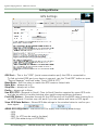
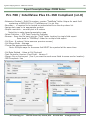
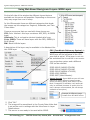
Settings Window
User Interface 2
Above are optional settings, not the software defaults.
Map Background Color—Able to switch map background color to Black or White. Suggest using
white for mapping, the black is useful for GPS—in field use.
Cursor Coordinate Units—changes the values at the bottom of the screen as you move the
“mouse cursor” around the screen. (has no effect on the maps or projections)
Area Measure Unit—changes the method by which the area of the surface and area of polygon
drawings are calculated.
Linear Measure Unit—changes the method of measuring distance. This will effect the measure
tools and how lines in drawing layers are calculated.
Above/Below Grade Units—changes the units in the “Drainage Window” “Profile” area only, giving you option of seeing your cut in “Feet” or “Inches”.
Zone Results Folder Name—is the “folder name” created when writing / creating new maps in
the “Merge Zone Results” window
Grid Results Folder Name—is the “folder name” created when writing / creating new maps in
the “Merge Grid Results” window
Current Season—adds the “year” to the folder name in “Merge Grid Results” & “Merge Zone Results” windows when writing / creating new maps.
Start Search for Sample Results in Field Folder—Check=start in “Field” folder you are working
No check = Start search in last folder
GK Technology, Inc. - 204 Fi h Street East, Halstad, MN - 855-458-3244 - www.gktechinc.com
Ag Data Mapping Solu on - ADMS User Manual
13
Settings Window
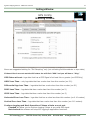
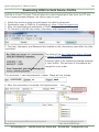
GPS Settings
GPS Port— This is the “COM” (serial communication port) the GPS is connected to.
To find out what COM port your device is connect, use the “Find GPS” button or open
“Device Manager” and look under “Ports (COM & LPT)”
Baud Rate— Set this value to match the GPS receiver output rate
Data Bits— always set to 8
Stop Bits— always set to One
Parity— always set to None
Use RTS/CTS—(Request to Send / Clear to Send) function required by some GPS units
and can be useful in trouble shooting other serial communications problems.
Find GPS Button— Searches through all the COM ports & all the BAUD rates looking for a
valid GPS signal. Function may not work if you are indoors and have no GPS signal.
View GPS Data Button— Shows GPS data strings in the window below to confirm you
have signal.
ADMS GPS REQUIRES— the source GPS to supply the following data strings
- GGA
- GSA
- RMC (or VTG can be used in its place)
- GST (this data string is OPTIONAL)
GK Technology, Inc. - 204 Fi h Street East, Halstad, MN - 855-458-3244 - www.gktechinc.com
Ag Data Mapping Solu on - ADMS User Manual
14
Settings Window
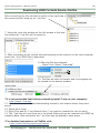
GPS Config
Warning Criteria
Above are suggested setting for “Soil Sampling” only (not collecting field boundaries or topo data)
If these Criteria are not met the GPS status bar will flash “RED” and you will hear a “Ding”
GPS Status at Least—logs data that has a GPS Signal of at least this or greater (ex-GPS Only)
HDOP Less Than— only logs data that has a value less than this number (ex-3.0)
Differential Age Less Than— logs data that has a value less than this number (ex-30)
PDOP Less Than— logs data that has a value less than this number (ex-3)
VDOP Less Than— logs data that has a value less than this number (ex-3)
Horizontal Error Less Than— logs data that has a value less than this number (ex-0.10 meters)
Vertical Error Less Than— logs data that has a value less than this number (ex-0.10 meters)
Continue Logging and Mark Operations if these criteria are not met.
Checked will allow you to continue logging if there is any valid GPS signal.
Not checked the software will stop ALL logging & application functions.
GK Technology, Inc. - 204 Fi h Street East, Halstad, MN - 855-458-3244 - www.gktechinc.com
Ag Data Mapping Solu on - ADMS User Manual
15
Settings Window
GPS Config
GPS Cursor
Above are optional setting, not software defaults.
Size—is in the number of “Pixels” not feet. (size preference is relative to your Screen Resolution)
Outside Line Width—is in number of “Pixels” wide
Line Color— set to your color preference. (think about background map colors-contrast is good)
Fill Color— set to your color preference. (think about background map colors-contrast is good)
For these settings to take affect. The “Map Window” or “Log & Sample” window must be closed
and re-opened if you are trying to adjust these settings with these windows open.
GK Technology, Inc. - 204 Fi h Street East, Halstad, MN - 855-458-3244 - www.gktechinc.com
Ag Data Mapping Solu on - ADMS User Manual
16
Settings Window
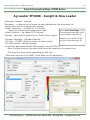
GPS Config
Above settings are recommended if working with one of these three GPS receivers.
To use these options you must have the “GSP Settings” tab in the “View GPS Data” mode. This
means that data is “STREAMING” across the viewing area of the screen. Then go to the “GPS
Config” tab either the General or Garmin setting.
Check on the data strings you want the device to put out.
Set the Hz rate (Data strings per second)
2 = 1 data string every 2 seconds or 1 string every 2 seconds
1 = 1 data string every 1 second or 1 string per 1 second
0.2 = 1 data string every 0.2 seconds or 5 strings per 1 second
If you want to change the baud rate check the box and adjust the rate.
Click the “Set” button
If this does not work you may have to check the “Use RTS/CTS” button in the “GPS Settings”
GK Technology, Inc. - 204 Fi h Street East, Halstad, MN - 855-458-3244 - www.gktechinc.com
Ag Data Mapping Solu on - ADMS User Manual
17
Settings Window
UTM Zone
Choose the correct zone for where you are working. One of the major drivers for what UTM you
use is the FSA—NAIP imagery. We suggest setting your UTM to match what the Government
has assigned for the Imagery. If you are in an area where there is no NAIP imagery, use the
UTM zone of the Landsat data that best fits your area. Questions here please contact your support staff at GK Technology Inc.
UTM—Acronym for “Universal Transverse Mercator”. A projected coordinate system that divides
the world into 60 north and south zones, 6 degrees wide. This is what everything is projected in
within the software. Being in the correct UTM zone is critical to ensure the location is accurate.
Other Notes on Projection and Units for ADMS.
ADMS supports Vector data (SHP) files in UTM or LAT/LON coordinate systems. All images coming in must be in UTM coordinate system. ALL UTM objects must have the units in METERS (for
Northing / Easting).
GK Technology, Inc. - 204 Fi h Street East, Halstad, MN - 855-458-3244 - www.gktechinc.com
Ag Data Mapping Solu on - ADMS User Manual
18
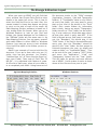
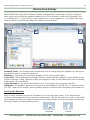
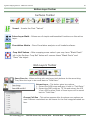
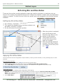
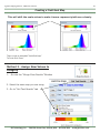
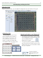
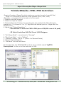
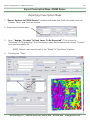
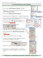
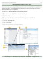
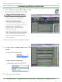
Window Dock Settings
Within ADMS there are many different window configurations. Depending on which unlock you
have there may be different panels available to you. At a minimum there will be Drawing Tools
(1.), Statistics (2.), Layer Info(3.), Layer Selection (4.), and Database (5.). By default the Layer
Selection panel is pinned open when the software first is started.
1.
3.
4.
2.
5.
Drawing Tools— The drawing tools window has tools to merge polygons together to create polypolygons as interior or exterior polygons.
Statistics—This panel will show layer statistics of the active surface layer.
Layer Info—This breaks apart the layers that are loaded into the software in three different categories: Drawings in Map, Surfaces in Map, and Images in Map. In this panel layers can be cleared,
made active, and re-ordered.
Layer Selection—This panel has the data tree in it along with the query tool and GPS.
Database—The database gives the user access to the database in a SHP file, or a attribute table
in a CSV. Data can be queried, sorted, added, deleted, and have math operations performed on it.
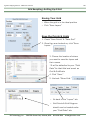
Docking the Windows
Each of these windows will have a thumbtack icon in the top right corner. If the thumbtack is
clicked on the window will be permanently docked open. This can be useful for certain types of data processing and allow for easier access to some of the toolbars. Once pinned open the map window and toolbars will automatically resize.
Unpinned
Pinned
GK Technology, Inc. - 204 Fi h Street East, Halstad, MN - 855-458-3244 - www.gktechinc.com
Ag Data Mapping Solu on - ADMS User Manual
19
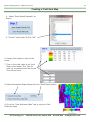
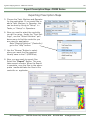
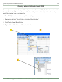
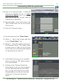
Window Dock Settings
These panels can also be docked inside each other or moved to a different location. This gives the
software users may options to fit their preferences.
To dock or move a panel first open and pin everything you want open permanently. Next click on
the panel you wish to move. For this example the statistics window will be used and get docked
under the Layer Info Panel. This allows the user to see all the layers that are loaded and allow for
easy visibility to layer statistics.
•
•
•
•
•
Click on Layer Info to open it followed by the thumbtack to dock it open.
Click on the Statistics to open the window over top of the Layer Info.
Left click on the window header to make a four way crosshair cursor appear.
Hold and drag the window out of the side to where you want it. In this example will want to
dock it under the Layer Info so drag it to the bottom of layer info. Once there it will show a
preview of it snapping in place.
Once you see it snapping in place let go of the cursor. It will then be docked in place.
After docking now all the layers are visible that are currently turned on within ADMS.
The histogram is easily visible
for the surface layer turned on
in the map window.
GK Technology, Inc. - 204 Fi h Street East, Halstad, MN - 855-458-3244 - www.gktechinc.com
Ag Data Mapping Solu on - ADMS User Manual
20
Window Dock Settings
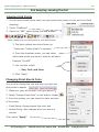
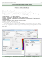
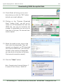
Resetting Window Dock Settings
Sometimes when working with different windows one will “disappear.” What actually happens is a
panel will get moved behind the main window and it can’t be accessed. Also, if the windows are in
a configuration that you aren’t happy with they can be reset.
•
•
•
•
•
CLOSE THE MAP WINDOW—This is a very important step. If the map window is open the settings will not work.
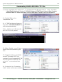
Go to the to toolbar above the startup window select Tools ► Reset Window Dock Settings
Click Reset Window Dock Settings
A window will appear that says “Done.”
Open the Map Window. All the panels will be docked the same way they were when the software was first installed.
GK Technology, Inc. - 204 Fi h Street East, Halstad, MN - 855-458-3244 - www.gktechinc.com
Ag Data Mapping Solu on - ADMS User Manual
21
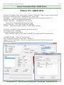
Top Map Toolbar
Map Window Toolbar
Zoom to Project Extents
- Zooms out to the full extent of all the layers that are
open.
Zoom to Rectangle
- Zooms to the user drawn rectangle on the map.
Zoom In – Re-centers the image to wherever you "Left Click" and zooms in on that area
("Right Click" to turn off tool).
Zoom Out –
Re-centers the image to wherever you "Left Click" and zooms out on that
area ("Right Click" to turn off tool).
Move
- "Left Click", hold down and drag on the map - when you release the "Left Mouse
Button", your image will move ("Right Click" to turn off tool).
Tape Measure -
Allows you to find distances and heading by left clicking around your
screen.
Print
- Takes you directly to the "Print Map" function.
GK Technology, Inc. - 204 Fi h Street East, Halstad, MN - 855-458-3244 - www.gktechinc.com
Ag Data Mapping Solu on - ADMS User Manual
22
Top Map Toolbar
Map Window Toolbar
Select Mode: Replace - Sets the mode of selection to add a single object for all the
select tools, allowing selection of a single item (of Active-”Drawing Layer”).
Select Mode: Add - Sets the mode of selection to add multiple objects for all the
select tools, allowing you to add multiple selections (of Active-”Drawing Layer”).
Select Mode: Subtract
- Sets the mode of selection to remove multiple objects for
all the select tools, allowing removal of multiple selections (of Active-”Drawing Layer”).
Clear Selection - Clears all the selected items (of Active-”Drawing Layer”)
Selected Objects - Shows you how many objects you have “Selected” in your
Drawing Layer.
Select With Click - Allows selection of a single item in the active layer, must choose
the "Select With Click" button for every object (of Active-”Drawing Layer”)..
Select By Rectangle
- Allows selection of multiple Points, Lines and Polygons by
drawing a “Rectangle” around them or intersecting with object (of Active-”Drawing Layer”)..
Select By Polygon - Allows selection of multiple Points, Lines and Polygons by drawing a “Polygon” around them or intersecting with object (of Active-”Drawing Layer”)..
Save Selected Objects to New Layer - Once you have selected your Points,
Lines and Polygons from a layer, you can "Save" these items to a newly named layer.
Multi Layer Map Math
- Opens a new page in which you can write scripts to perform
different functions and apply algorithms on your selected layers.
Multiple Output Map Math - Consultants only option. Opens a new page in which
you can write scripts to perform different functions and apply algorithms on you selected layers. This function will allow you to create “Multiple Output maps” in one click from a script.
Quick Math - Consultants only option. Allows scripts to be quickly run from a dropdown
menu that have previously been saved as a DLL.
GK Technology, Inc. - 204 Fi h Street East, Halstad, MN - 855-458-3244 - www.gktechinc.com
Ag Data Mapping Solu on - ADMS User Manual
23
Bottom Layer Toolbar
Bottom Toolbar—Basic Buttons
Remove Layer - Removes the selected layer from the map (does not DELETE layer).
The layer can be turned on again later.
Zoom To Layer - Zooms to the extent of the selected layer.
Bring to Front
Send to Back
- Moves the selected layer to the front of (or on top) all layers.
- Moves the selected layer to the back of (or bottom) all layers.
Save Changes
- Quickly saves any changes made to the selected layer.
Layer Visibility On/Off -
Turns the visibility of the layer on and off.
Address Bar and Active Layer
Cursor Coordinates—Values will be in either Latitude / Longitude
Easting of the “Cursor” location (adjusted in the settings)
or
UTM—Northing /
These values only show when drawing a LINE or POLYGON
LSLeng: Line Segment Length = distance from your last click to cursor.
LS Bear: Line Segment Bearing = degrees for your last click to the cursor
Total Len: Total Length = length of line or polygon drawn from first click to cursor
FP Bear: is First Point Bearing in Degrees
Value on the RIGHT is the distance across the “Map Window” (East to West)
The data in RED—is the
ACTIVE LAYER
— VERY IMORTANT !!!!!
This line tells you what layer you are actively working on and what layer the buttons will affect or change.
GK Technology, Inc. - 204 Fi h Street East, Halstad, MN - 855-458-3244 - www.gktechinc.com
Ag Data Mapping Solu on - ADMS User Manual
24
Bottom Layer Toolbar
Drawings Buttons
Change Draw Style
- Changes the line and point attributes (color, sizes and fill).
Thematic Draw Settings
- Opens a new window which allows the user to change color
themes, adjust the number of color ranges, view statistics of the color ranges, and fill and size the
points and lines.
Change Label Settings - Allows the user to view data from the objects data table in the
viewing window as a label. Also allows label size, font, and color adjustment.
or
or
Draw New Object - Once selected, you may draw a polygon, line or
point (left clicking to draw and right clicking to end lines and polygons.
Decompose a selected PolyPolygon to its Component Polygons - To
use this button “select” a PolyPolygon then click the button. Suggest doing a “Save As” and rename
the drawing layer. This will save the Polygon in it’s component state.
Move Vertices of Selected Object - Is a TOGGLE on/off button that allows you to
move the Vertices of Polygons and Lines. Object must be “selected” before using this button.
Draw a Circle - Once selected, left click and hold down in the center of the object and drag
to the desired diameter and release to create a circle polygon.
Drawing Properties
- Double clicking on an object, opens the properties of that
item.
Intra-Layer Math
- Allows use of simple mathematical functions on a column of the data
base.
Delete Selected Objects
- Once an object of this layer is selected, this will delete the
selected objects. Changes must be saved to be made permanent.
GK Technology, Inc. - 204 Fi h Street East, Halstad, MN - 855-458-3244 - www.gktechinc.com
Ag Data Mapping Solu on - ADMS User Manual
25
Bottom Layer Toolbar
Surfaces Toolbar
Change Color Theme - Changes the color pallet used on the selected layer.
Thematic Color - Opens a window to view image statistics, adjust color
themes, number of zones, and adjust zone sizes automatically or manually.
Load Fixed Thematic Table - Applies a color theme that has been previously
created to active layer.
Smoothing Filter - Combines pixels of the image creating a smoother image.
Fill Filter - Fills null values in and around the image by stretching or copying
the value of the nearest pixel.
Apply mod to Selected Polygon - Allows use of simple mathematical functions on selected layers using a combination of Polygons with Raster.
Trim End Values - Allows the change or deletion of values above, or below, a
given value (making all the removed values equal to the trim value). Deleted
values create a hole that will need to be filled.
Surface Properties - Tools to change “Units” and adjust the Geo Reference
and Resolution of the Surface.
Crop Raster to Selected Polygon - To use this tool, FIRST SELECT A POLYGON. Once the polygon is selected and you have reselected the surface layer
you want to cut to, this button will remove all the image outside of the selected
polygon. (“Just this Layer” Don’t forget to SAVE or SAVE AS!) (“All Visible” cuts
all loaded surfaces and AUTO SAVES — BE CAREFUL)
Reduce Boundary Effect - Will go around the field boundary looking in X—
Meters and stretch that value over the selected distance.
GK Technology, Inc. - 204 Fi h Street East, Halstad, MN - 855-458-3244 - www.gktechinc.com
Ag Data Mapping Solu on - ADMS User Manual
26
Bottom Layer Toolbar
Surfaces Toolbar
Invert - Inverts the Pixel “Values”
Intra-Layer Math - Allows use of simple mathematical functions on the active
layer.
Correlation Matrix - Runs Correlation analysis on all loaded surfaces.
Crop Null Values - After cropping some raster's you may have “Blank Pixels”
left in the Surface. Crop Null Values will remove these “Blank Pixels” and
“Save” the object.
Web Layers Toolbar
Save/Save As - When working with web layers both buttons do the same thing.
They allow the layer to be saved back to “Field Data.”
Extract Layer - This button gives two options.
1. Extract the RGB image and save it back to “Field Data.”
2. Extract the RBG image as TIF file and extract the VIS
VI as a GRD surface. Both of these layers will be saved
back to “Field Data.”
Choose Cell Size - This option appears after the above save options are
used. Different resolutions can be chosen for the final image/extracted surface.
GK Technology, Inc. - 204 Fi h Street East, Halstad, MN - 855-458-3244 - www.gktechinc.com
Ag Data Mapping Solu on - ADMS User Manual
27
Bottom Layer Toolbar
Multi-Band Image Buttons (TIF & BMP)
Multi-Band Image (SID & JP2)
Image Properties - Allows the geo-referencing of an image to be adjusted.
Multi-Band Layer Display - Select which bands of light and what order they
are displayed.
Equalize Image Display - Lighten or equalize the bands of light being displayed.
Reset Color Adjustment - Move the color bands back to their original settings.
Darken - Adjusts the brightness of the displayed image darker.
Brighten - Adjusts the brightness of the displayed image brighter.
Single Band Extraction - Lets individual bands be extracted from an image.
These are the bands that are adjusted in the “Multi-Band Layer Display”
Visual Index - Applies different vegetative indices depending on the type of
image and bands available. For RGB images the option will be “RGB VI” (Red,
Green, Blue Vegetative Index). If the image is CIR or has an inferred band
there will be a RNDVI and GNDVI option.
Extract From SID/JP2 – *This is a consultants package only option. To use
this button, must SELECT a boundary first. This button will give a list of different extraction types and after extraction they will be saved back to “Field Data.” This button eliminates the need to extract a TIF from SID/JP2 first.
GK Technology, Inc. - 204 Fi h Street East, Halstad, MN - 855-458-3244 - www.gktechinc.com
Ag Data Mapping Solu on - ADMS User Manual
28
Bottom Layer Toolbar
Images
-
Re-Sample Display Modes
Both images and surfaces can have their appearance adjusted by changing the re-sample
modes on the bottom toolbar. This affects only how the data is displayed and does not
affect processing.
NNeighbor—Selects the value of the nearest point and does not consider the value of neighboring cells
Bilinear—Linear interpolation is done in one direction and then again in another direction
Cubic—Takes 16 pixels into account and generally has a smoother appearance than Bilinear or NNeighbor
interpolation
Transparency Settings
Both Images and surfaces can have their transparency adjusted for visual purposes.
The number is in a Percentage (%).
*Note: Windows 7 there are issues with the transparency settings for surfaces. Therefore, if layering with
an image the image should be brought to the front and it’s transparency should be adjusted.
GK Technology, Inc. - 204 Fi h Street East, Halstad, MN - 855-458-3244 - www.gktechinc.com
Ag Data Mapping Solu on - ADMS User Manual
29
Drawing Layers (Polygons, Lines, & Points)
In Ag Data Mapping Solution, there are 4 ways to create/add Drawing Layer Data. Drawing Layer Data can consist of Boundaries, A-B Lines, Tile Lines,
Sample Points, Sample Grids, As Applied Maps, some Application Maps &
many more files. All the below examples are using the “Map Window”. Some
other windows may not have the same functionality.
1. Import from Another Source
2. Extract Drawing Layers from a Mass Collection
(FSA-CLU Field Boundaries/Roads/Yield Data)
3. GK Drawing Tools-Hand Drawing
4. Collect with GPS Using Ag Data Mapping Solution
- Importing from Another Source
Polygons (boundaries), lines and points that have been collected using
another source such as a tractor, pickup, ATV or hand drawn (in other software), all of these would be coming from a different software package. If
these files are coming from another software package, export the files out
as Shapefiles (.shp) and save them into the appropriate Grower / Farm /
Field (C:/GKData/xxx/xxx/xxx). If you are copying these Shapefiles, make
sure you get all the extensions of the shape file (Min requirement .shp, .shx
& .dbf). Paste them in to the appropriate Grower / Farm / Field
(C:/GKData/xxx/xxx/xxx). ADMS does handle “Imports” from certain
sources. Generally, you need to have the original data cards from the equipment. Find out by clicking on the “Import” tab while using “Map Window”.
GK Technology, Inc. - 204 Fi h Street East, Halstad, MN - 855-458-3244 - www.gktechinc.com
Ag Data Mapping Solu on - ADMS User Manual
30
Drawing Layers (Polygons, Lines, & Points)
Extracting Drawing Layers from a Mass Collection
(FSA - CLU Field Boundaries/Roads/Yield Data)
To use this function you must “SELECT” the Drawing object you want to “SAVE” or
“CREATE”
There are three ways of selecting these objects. To use them you must first turn on
the drawing layer that contains the objects to be saved (CLU-Yield Data-Roads-Topo
Data). Key to this process is watching your “ACTIVE LAYER on the Bottom Toolbar”
1. Select by Click—Simply left clicking on or in the object
2. Selecting by Area—Basically drawing a boundary around the object.
3. Selecting by Database—Using the “Database” tab and choosing the object out of
the dataset.
The next examples will explain these functions.
-Selecting by Click—(Example with “POLYGONS”)
1. For this example, turn on FSA (CLU) field boundaries (Multiple SHP file Object).
2. Select “Select Mode Replace”
& “Select with Click”
on the top toolbar.
** Note: This is selected by default when software starts **
3. “Left Click” inside the Polygon (Boundary) you want. By holding down the “Ctrl” key
you can select multiple objects.
4. Note that the Polygons have turned “Lime Green” showing they have been selected.
5. Top toolbar -note number of
“Selected:” objects
6. On the TOP TOOLBAR, select
“Save Selected Objects to a
New Layer”.
7. This will open into a “Save” window.
8. Notice it is saving back into your
“Field” level data every time.
9. Name the object & click “Save”.
GK Technology, Inc. - 204 Fi h Street East, Halstad, MN - 855-458-3244 - www.gktechinc.com
Ag Data Mapping Solu on - ADMS User Manual
31
Drawing Layers (Polygons, Lines, & Points)
Extracting Drawing Layers from a Mass Collection
(FSA - CLU Field Boundaries/Roads/Yield Data)
Selecting by Area—Example with “POINTS”)
1. For this example, turn on Yield Data, Veris Data or Topo Data as “Points” Shape file.
2. Select the “Select Mode Add” off the top toolbar.
3. Then select either “Select by Rectangle” or “Select by Polygon”
4. Then follow the directions below the top Toolbar.
5. Note that the objects have turned “Lime Green” showing they have been selected.
6. Top toolbar -note the number of “Selected:” objects.
7. On the TOP TOOLBAR, select “Save Selected Objects to a New Layer”.
8. This will open into a “Save” window.
9. Notice it is saving back into the “Field” level data every time.
10. Name the object (you MUST Re-Name the object) & click “Save”.
Selected by “POLYGON”
Selected by “RECTANGLE”
GK Technology, Inc. - 204 Fi h Street East, Halstad, MN - 855-458-3244 - www.gktechinc.com
Ag Data Mapping Solu on - ADMS User Manual
Drawing Layers (Polygons, Lines, & Points)
Extracting Drawing Layers from a Mass Collection
(FSA - CLU Field Boundaries/Roads/Yield Data)
Selecting by Database—(Example with “POINTS”)
1. For this example, turn on the yield data points.
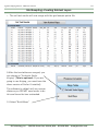
2. On the bottom left corner of the screen, click on ”Database” tab.
3. This will open the database of the “Active Drawing Layer” or the last active SHP.
4. Selection Methods :
A. By “Left Clicking” on the gray cell on the left side of the table. (Note the Database Row highlights and the Map Object turned “Lime Green” showing they
have been selected).
B. By holding down the “Shift” key and left clicking a row further down in the database, you can select groups of objects.
C. By holding down the “Ctrl” key and left clicking a row and another row, you
can select multiple individual objects throughout the database.
D. Using the DB Operations : “Select by Query”, you can select a “Column” and
Query out objects (>,<,=,>=,<= (on numeric columns)) and (=,<> (on
character columns)), put in your values and click “Run Query”.
NOTE: The “Object Selected:” in the upper left hand corner of the Database
window, this will tell you how many objects are selected in the Database.
5. On the TOP TOOLBAR, select “Save Selected Objects to a New Layer”.
6. This will open into a “Save” window.
7. Notice it is saving back into the “Field” level data every
time.
8. Name the object (you MUST Re-Name the object)
& click “Save”.
GK Technology, Inc. - 204 Fi h Street East, Halstad, MN - 855-458-3244 - www.gktechinc.com
32
Ag Data Mapping Solu on - ADMS User Manual
33
Drawing Layers (Polygons, Lines, & Points)
GK Drawing Tools - Hand Drawing (Polygons)
•
•
Using the hand drawing tools, you will need to have a “Layer” turned on that you can
Trace, or Mark, on top of for geo-referencing purposes. (Accurate, high quality data is
needed).
Look at drawing Polygons & Merging Interior / Exterior Polygons (Poly-Polygons)
- Polygons (Drawing—Field Boundaries)
1. Hand Drawn is done using either field collected data points or 1-3 meter aerial-images.
Both giving geo-referenced data to trace.
2. Zoom into the field as close enough to see and draw all details.
3. At the bottom of the “Data Tree” Select “Create New Layer From Template”.
4. Select “Boundary” from the template list.
5. In the “Data Tree” check the “Boundary.shp”.
Note: ACTIVE LAYER—Below the Map Window — Field:Name
Layer:Boundary.shp
6. On the “Bottom Toolbar” click on the “Draw New Object” button .
7. In the map window area, follow the instructions at the top of the “Map Window”
Drawing Tool Selected, Left Click each Point, to Define the New Object, Right Click to Finish
Note: if you make a mistake while drawing—Hold Down the “Alt” - Key and “Left Click” to undo last
point.
8. “Right Click” to finish the Polygon.
9. If there is a second & third boundary (interior or exterior) repeat 6—8.
The next page will create the “interior—exterior” polygons
10. Once finished drawing the “Boundary”, click ”Save” on the bottom tool bar.
GK Technology, Inc. - 204 Fi h Street East, Halstad, MN - 855-458-3244 - www.gktechinc.com
Ag Data Mapping Solu on - ADMS User Manual
Drawing Layers (Polygons, Lines, & Points)
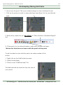
GK Drawing Tools - Merging Boundaries
Exterior / Interior
Polygons (Creating Poly-Polygon)
1. Turn on your Multiple Polygon Boundary.
2. Open the “Database” tab (lower left corner).
3. Click on the row tabs in the “Database” that contain exterior polygons, this will highlight the whole row and the object will highlight
“Lime Green” in the map window.
4. Click on the “Drawing Tools” tab on the Right side.
5. Click “Add Selected Polygons” in the “Exterior Polygons” area. (If
incorrect objects selected, click “Clear Polygon Collections”).
6. Click on the row tabs in the “Database” that contain interior polygons, this will highlight the whole row and the object will highlight
“Lime Green” in the map window.
7. Click the “Add Selected Polygons” in the “Interior Polygons” area.
8. If you select the incorrect object, click “Clear Polygon Collections”.
9. Once the “Multi-Polygon Builder” windows are populated correctly. Go to the “Destination Layer” drop down and Select the SHP location you want to save the “Merged Boundary” (poly-polygon). Note:
you may want to save the new object to a “NEW LAYER”
10. With the correct Layer, click “Merge Interior and Exterior Polygons to
Poly Polygon” in “Exterior Polygons”
area.
11.Notice the “Database” has gone to just
ONE object in the table.
12.IT IS VERY IMPORTANT THAT
THESE OBJECTS ARE DRAWN &
LISTED CORRECTLY.
13.If all is correct, click ”Save” under the
“Draw Polygons” area.
Note: The “Save” is a Save As
process so you will have the
option to “Re-Name”
GK Technology, Inc. - 204 Fi h Street East, Halstad, MN - 855-458-3244 - www.gktechinc.com
34
Ag Data Mapping Solu on - ADMS User Manual
Drawing Layers (Polygons, Lines, & Points)
GK Drawing Tools - Hand Drawing (Lines & Points)
- Lines
1. Typically, we like to draw this data off of either field collected data points or 1-3
meter ortho-images (Geo-Referenced very well).
2. Zoom into the field as close as possible (all parts of the field must be visible).
3. At the bottom of the “Data Tree” Select “Create New Layer From Template”.
4. Select “Tile Line” from the list.
5. Check the “Tile Line”.
6. Click on the “Draw a New Object” button on the “Bottom Toolbar”
7. In the Map Window area, follow the instructions at the top.
Drawing Tool Selected, Left Click each Point, to Define the New Object, Right Click
to Finish
Note: if you make a mistake while drawing—Hold Down the “Alt - Key” and “Left
Click” to undo last point.
8. For the Polygon & Line tool, “Right Click” to finish the object.
9. Repeat the previous 3 steps adding all the lines you need.
10. Click ”Save” on the “Bottom Toolbar”.
- Points (Single Point Drop)
1. Typically we like to draw this data off of either field collected data points or 1-3
meter ortho-images (Geo-Referenced very well).
2. Zoom into the field as close as possible (normally want to see the whole field).
3. At the bottom of the “Data Tree” Select “Create New Layer From Template”.
4. Select “Sample Points” from the list.
5. Check the “Sample Points”.
6. Click on the “Draw a New Object” button on the “Bottom Toolbar”
7. Left click where the point is to be placed.
8. Repeat the previous 2 steps adding all the points you need.
9. Click ”Save” on the “Bottom Toolbar”.
GK Technology, Inc. - 204 Fi h Street East, Halstad, MN - 855-458-3244 - www.gktechinc.com
35
Ag Data Mapping Solu on - ADMS User Manual
36
Drawing Layers (Polygons, Lines, & Points)
GK Drawing Tools - Hand Drawing (Multi-Point)
- Points (Draw Multiple points)
There are time you may want to mark many points on a field. In these cases you will NEED to have a
“Surface.grd” or “Surface.bmp” built for the field. In this example “Zones ID.grd”
1.
2.
3.
4.
5.
6.
Select your Grower / Farm / Field
Check on the Surface.grd (ex. Zones ID.grd) (This tool will NOT work without a SURFACE Checked)
At the bottom of the “Data Tree” Select “Create New Layer From Template”.
Select “Sample Points” from the list.
Check the “SamplePoints.shp” in the “Data Tree”
Click “Multi Point Draw Tool” on the bottom toolbar below your map window. (this is a toggle on/off)
7. Click out the points in the order you would want them sampled and in the spot you want sampled.
8. When you are finished deselect the “Multi Point Draw Tool” your new points will automatically save.
9. You now should have your custom points that look similar to the image below.
10. Once finished click “Save” on the bottom toolbar.
GK Technology, Inc. - 204 Fi h Street East, Halstad, MN - 855-458-3244 - www.gktechinc.com
Ag Data Mapping Solu on - ADMS User Manual
37
Drawing Layers (Polygons, Lines, & Points)
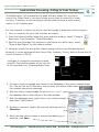
Collect with GPS Using Ag Data Mapping Solution (Map Window)
1. Turn on all layers you want to view for background maps
2. Check on “EXISTING” “Boundary” or “Ditch Line” or “Sample Point” if you want to add
to Existing data.
- Connect GPS
1. Go to the “GPS Mark” tab.
2. Click “Connect GPS”.
3. For Topography collection, check “Start Logging”.
NOTE: if “Logging” is “ON” you WILL NOT be able to turn
on or off Layers or Data.
- Marking Data
1.
2.
3.
4.
5.
Go to the “Mark” tab.
For New Shape File “Create Layer From Template”.
For “Existing SHP” files, Click “Save To Layer”
Click “Start”.
“Pause” will allow you to drive around un-drivable areas - “Continue” button will appear.
6. Click on “Stop” once you have reached your finish
point.
7. The object will automatically “Save”.
8. Repeat steps 1-6 drawing in all the Interior & Exterior
Boundaries for this field.
9. To view acres, make sure the object is the “Active Layer”.
“Double Click” on the object - or click on the “Database” tab for acres.
10. For fields with no interior boundaries, you are finished.
11. For Interior Boundaries, go back two pages “Exterior/Interior Polygons
(Creating PolyPolygon)” section
** More GPS information in the “Using GPS Controls” Section of the manual. **
GK Technology, Inc. - 204 Fi h Street East, Halstad, MN - 855-458-3244 - www.gktechinc.com
Ag Data Mapping Solu on - ADMS User Manual
38
Drawing Layers (Polygons, Lines, & Points)
Decomposing a Poly-Polygon
Some boundaries may come in or have been built as Poly-Polygons. These interior polygon may need to
be removed. These instructions will show you how to do this. This example will show how to remove 2
tree rows from a field.
1. Turn on our Poly-polygon boundary (note I turned on NAIP for this example)
2. Click inside the Boundary (making it a “Selected Object” - Lime Green)
3. On the bottom toolbar click on the “Decompose a selected PolyPolygon to its
component Polygons”
4. This is a good time to do a “Save As” & Re-Name (ex. Boundary 2012.shp)
5. Make sure the active layer is Boundary 2012.shp
6. Select the polygons to remove. (either by Clicking in them or using the Database)
7. Click on “Delete Selected Objects” button on bottom toolbar.
8. Click “Save” on the bottom toolbar.
Boundary as Poly-Polygon
Only has 1 Database entry
Boundary as Multiple Polygon
Has multiple database entries
Note : The Database of each object.
GK Technology, Inc. - 204 Fi h Street East, Halstad, MN - 855-458-3244 - www.gktechinc.com
Ag Data Mapping Solu on - ADMS User Manual
39
Drawing Layers (Polygons, Lines, & Points)
Moving Vertices or Moving Points
Some Points / Lines / Polygons may have imperfections in one or two areas that are drawn incorrectly.
These objects may not need to be totally redrawn. There is a tool for moving these vertices and points.
These instructions will show you how to do this. This example will show how to remove 2 tree rows from
a field boundary.
1. Turn on Points / Line / Polygon SHP file that needs to be edited (polygon in this example)
2. Click on or in a single object to edit (making it a “Selected Object” - Lime Green)
3. Bottom toolbar click on the “Move Vertices of a Selected Object” button to turn it “On”.
Note: This is a “Toggle On/Off button”
4. Move your Cursor over one of the “Vertices” or “Point” you will get a “4-Way Pointer” and Left Click.
Note: Lines and Polygons will break down to show all vertices.
5. To move one of “Vertices” or a “Point” and left click hold and move
Note: Holding the “CTRL” button and a “Right Click” will add a vertices
Holding the “ALT” button and a “Right Click” will delete a vertices
6. Click on the “Move Vertices of a Selected Object” button to turn it “Off”.
7. Repeat steps 2-6 as needed on any other object in this SHP file.
8.Click “Save” on the bottom toolbar.
Make sure you “Turn Off” the “Move Vertices” (shown below)
GK Technology, Inc. - 204 Fi h Street East, Halstad, MN - 855-458-3244 - www.gktechinc.com
Ag Data Mapping Solu on - ADMS User Manual
40
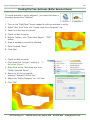
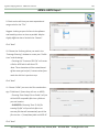
My Notes
GK Technology, Inc. - 204 Fi h Street East, Halstad, MN - 855-458-3244 - www.gktechinc.com
Ag Data Mapping Solu on - ADMS User Manual
41
My Notes
GK Technology, Inc. - 204 Fi h Street East, Halstad, MN - 855-458-3244 - www.gktechinc.com
Ag Data Mapping Solu on - ADMS User Manual
42
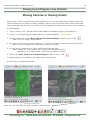
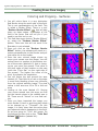
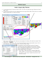
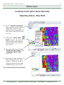
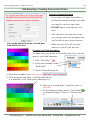
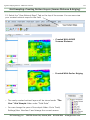
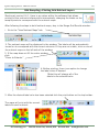
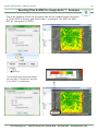
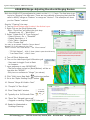
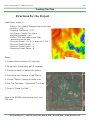
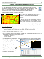
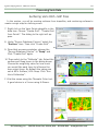
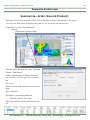
Quick Notes For Satellite Imagery
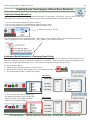
Creating Boundaries and Guidelines
1.
2.
3.
4.
Draw a field boundary or save it from a CLU file. Refer to creating boundaries section.
Turn on a NAIP image (County Data)
Create a new line file.
Draw reference lines from the NAIP image. This will be used to help georeference the satellite imagery.
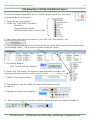
Selecting Polygon - Boundary
1.
2.
3.
4.
5.
6.
7.
A Boundary is needed for this process. Refer to the creating boundaries section to create a Boundary.
Turn on Boundary.shp and make sure it is the active layer.
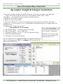
Go to the “Automated Zone Creation” Tab—Click “Set Selection Parameters”
Click inside the Boundary.shp polygon in the “Map Window”
The object will appear “Lime Green”.
Go to “Automated Zone Creation” tab—Click “Set Selected Boundary”
Go to the “Automated Zone Creation” Tab
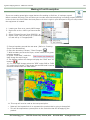
Cutting the Raster
1.
2.
3.
4.
5.
6.
Turn on All the Satellite images you want under (Imagery Tab).
Turn on the Guidelines that were created.
“Automated Zone Creation” Tab-Click on the Image Date to extract
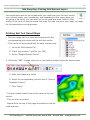
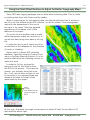
Choose the “Extraction Type” Red NDVI=Vegetation/NIR=Bare Soils
Click “Extract Images”
Use the Alignment Arrows to move Image (if needed) according to
guidelines
7. Choose “Desired Number of Zones”
8. Click “Finish” (Repeat 2-7 for all the Images)
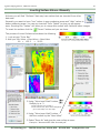
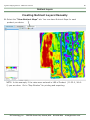
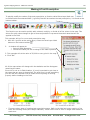
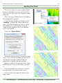
Coloring & Zoning Raster
1. Make sure your zone.grd is the active layer.
2. Useful tools at this time (if needed)
• “Reduce Border Effect”
• “Trim End Values”
• “Invert”
3. Click on “Smooth Filter” 5x5 - two times
4. Turn all images to be merged. Open Multi Output Map Math
5. Open “Average Of All Layers” script => Compile => Run
6. “Save As” Zones.grd
7. Click on “Thematic Color”
8. Adjust “Number of Ranges” to desired zone #
9. Adjust the settings like the window to the right
10. Normally use “2 Std Dev” or “K Means”.
11. Mouse over the “Color Chips” to adjust and use the “Scroll
Wheel” on the mouse for custom coloring.
12. When finished, click “Apply”.
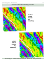
Saving for—Soil Sampling
1. Right click on the file name.grd in the data tree and select
save as BMP (most soil samplers) /// save as Google Earth
KMZ /// Or go to “File” & “Print Map” & “Print Map to Bitmap”
GK Technology, Inc. - 204 Fi h Street East, Halstad, MN - 855-458-3244 - www.gktechinc.com
Ag Data Mapping Solu on - ADMS User Manual
43
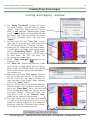
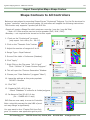
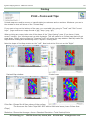
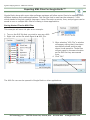
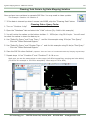
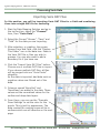
Creating Zones From Imagery
For this section of the help guide, we will be looking at Extracting and Handling Imagery.
In the reference to “Handling” Imagery, we refer to colorization and zone creation. We will
be working in the New Map Window, but many of these tools will carry across into other
windows in Ag Data Mapping Solution.
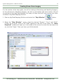
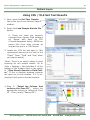
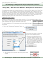
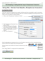
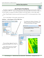
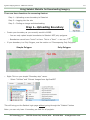
1. Start up Ag Data Mapping Solution and select the “Map Window”
button.
2. When the “Map Window” opens, select the desired “Grower”, “Farm” and “Field”.
If they do not exist, click on the “New” buttons to the left of the name. An “Input
Required” window will open up in the middle of the screen to enter the new name, do
so, and click “Apply”. Now you have your field selected.
GK Technology, Inc. - 204 Fi h Street East, Halstad, MN - 855-458-3244 - www.gktechinc.com
Ag Data Mapping Solu on - ADMS User Manual
44
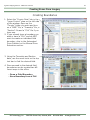
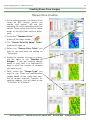
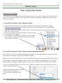
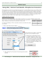
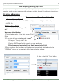
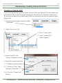
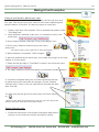
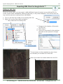
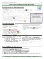
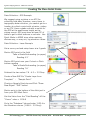
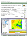
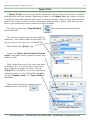
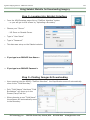
Creating Zones From Imagery
Creating Boundaries
1. Select the “County Data” tab in the
“Layer Control” area on the left side
of the window. Open up the
“County” folder you want and turn
on a “NAIP” file, a “Township” file, a
“Section” file and a “CLU” file if you
have one.
2. If you already have a boundary created or have a “CLU” and do NOT
want to create an individual field
boundary, skip to the Automated
Zone Creation or the Manual Zone
Extraction section.
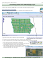
3. Using the Township and Section
data, use the zoom tools on the top
tool bar to find the desired field.
4. Once zoomed to the desired field,
boundaries can be created two different ways in the office:
- Draw a Field Boundary
- Save Boundary from a CLU
GK Technology, Inc. - 204 Fi h Street East, Halstad, MN - 855-458-3244 - www.gktechinc.com
Ag Data Mapping Solu on - ADMS User Manual
45
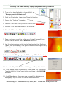
Creating Zones From Imagery
Creating Boundaries
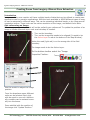
Hand Draw a Field Boundary
1. Make sure all the correct Grower, Farm, Field
data is selected and go to the bottom of the
“Data Tree” window and click on “Create New
Layer from Template” and select “Boundary”.
2. You will see the “Boundary” file you created
under the “Field Data” tab. Check the box in
front of the file name “Boundary.shp”, this
will make it the Active Layer.
3. Go down to the bottom tool bar and
the “Draw New Object” button.
select
4. Once this is selected, “Left Click” on the field
edge. Notice the blue line dragging behind the
cursor. The line will not draw until you “Left
Click” again at your next location (If you mark a
point at an incorrect position, hold down the “ALT” key
and left click to undo your last point marked). Once
you finish going around the field, “Right Click”
to complete the drawing. When you “Right
Click”, the software will close the boundary
by snapping the line back to the first point
marked.
a) Take note that as you draw a line, there
is a tool at the bottom – center of the
screen to help you. Giving you the line
lengths and headings to help guide you.
5. Once you have finished creating your
boundary, save the boundary by selecting
“Save” on the bottom toolbar. This will
open a save window - click on “Save”.
GK Technology, Inc. - 204 Fi h Street East, Halstad, MN - 855-458-3244 - www.gktechinc.com
Ag Data Mapping Solu on - ADMS User Manual
46
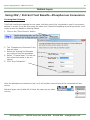
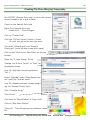
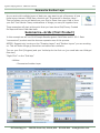
Creating Zones From Imagery
Creating Boundaries
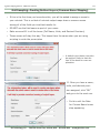
- Save Boundary from a CLU
1. Make sure the bottom active layers
has the address of the CLU.
Example- Layer: Norman CLU.shp
2. You need to select the polygon of
the field you want to save. You will
do this by clicking on the “Select
Mode Replace” on the top tool
bar and click inside of the polygon;
it will appear Light Green to show
it’s selected (Hold down your “Ctrl”
key to select multiple objects).
Note: the “Selected” on the top
toolbar. Should match the # of
objects selected.
3. Select the “Save Selected
Objects to New Layer” on the
upper toolbar. Make sure you are
saving in the correct location.
“Name” the object (ExampleBoundary FSA.shp) and “Save”.
GK Technology, Inc. - 204 Fi h Street East, Halstad, MN - 855-458-3244 - www.gktechinc.com
Ag Data Mapping Solu on - ADMS User Manual
47
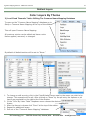
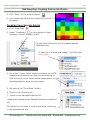
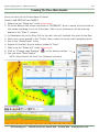
Creating Zones From Imagery
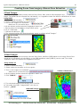
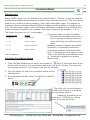
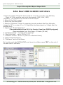
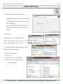
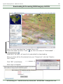
Creating Boundaries—Boundary Creation From Mass Collection
With some tools within ADMS boundaries can automatically be generated.
To automatically generate a boundary a point data collection is needed. This can be anything as
long as it’s point data. A few good sources are:
• Yield Data
• Elevation Survey Data
• As-Applied Data
Make sure there are now outlier points in the collection otherwise this process will take much
longer to run.
*Note: If yield is being used and has been cleaned up some of the data around the edge of the
field may be missing and the boundary will be inaccurate. In this situation consider exporting the
raw data for the purpose of boundary creation.
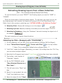
1. Turn on a data points file (SHP or CSV).
2. Right Click on the field in the data tree and
select “Generate Boundary.”
3. After that is selected the “Generate a Boundary from Points” window will appear. This window gives instructions along with different options of how the new boundary will be created.
The two options on this window are the
“Smoothness” and “Subset” values.
•
•
•
•
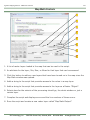
Smoothness Value: How close the boundary
follows the original points. The lower the value
the smaller the search radius will be.
Subset Value: How many points are used out
of the whole collection. (e.g. If the subset value is set at 3, every 3rd point will be used
during the calculation. Likewise, if it’s set at 20
it will use every 20th point.)
The boundary routine can be run multiple
times before saving the final boundary. This
allows you to adjust the smoothness and subset values.
It is recommended to keep the subset value so
it uses less then or equal to 10,000 points.
GK Technology, Inc. - 204 Fi h Street East, Halstad, MN - 855-458-3244 - www.gktechinc.com
Ag Data Mapping Solu on - ADMS User Manual
48
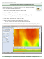
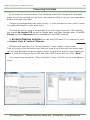
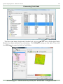
Creating Zones From Imagery
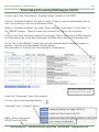
Creating Boundaries—Boundary Creation From Mass Collection
4. The smoothness and subset values will automatically be set by the software, but can be adjusted to change how the boundary follows the points.
5. Click “Run Boundary Routine”
6. Adjust the “Output File Name” if needed. If the name is changed make sure the *.shp extension stays on. Otherwise the boundary will not be recognized in the software.
7. Click “OK”
8. The polygon will be saved back to the data tree with the
entered file name.
Final adjustments can be made to the boundary using the “Move Vertices”
tool on the bottom toolbar.
• Select inside the boundary to turn it green.
• Select “Move Vertices of Selected Object.”
• Hover over the vertices and left click and hold to move them.
• After all vertices are moved click the “Move Vertices of Selected Object”
button again to turn it off.
• Save changes.
GK Technology, Inc. - 204 Fi h Street East, Halstad, MN - 855-458-3244 - www.gktechinc.com
Ag Data Mapping Solu on - ADMS User Manual
49
Extracting Images From NAIP
FSA—National Ag Imagery Program (NAIP) supplies us with high resolution .sid & .jp2
images. Typically 1 & 2 meter resolution. These instructions will walk you through
converting a small area into a .tif format to create a surface for making “Zones”. Keep
in mind there is not a “NIR” channel in most of this data. So we are working with the
“Red / Green / Blue” spectrum of visible light.
1. Turn on your “Boundary.shp”
- Note: you must be zoomed to the “Field”
2. Go to the “County Data” Tab
3. Turn on a NAIP image.sid (or .jp2)
4. Right click on the “NAIP Image.sid” name
5. Select “Extract Current View (SID/JP2)
6. Go to your “Field Data” Tab
•
•
Refresh the data tree
Open “Images/NAIP” Folder
7. Check on the new “County NAIP.tif”
make it the active layer (in RED)
8. Follow the image extraction instructions
Using - “Manual Extractions”
Consultant Users:
1. Turn on your “Boundary.shp”
- Note: you must be zoomed to the
“Field”
2. Go to the “County Data” Tab
3. Turn on a NAIP image.sid (or .jp2)
4. Click the extract from SID/JP2 icon
5. Several different options will appear in a
list.
6. Choose the appropriate extraction method
7. Go to the “Field Data” tab
• Refresh the data tree
• Open “Images/NAIP” Folder
8. The extracted file will have an extension
on it to define the extraction type
(ex: _Red, _RGB_VisVI)
GK Technology, Inc. - 204 Fi h Street East, Halstad, MN - 855-458-3244 - www.gktechinc.com
Ag Data Mapping Solu on - ADMS User Manual
50
Extracting Images From Web Layers
Starting at ADMS version 7.0.0 there is added functionality to give users access to web
based background imagery.
In order to use these options, the computer must have an active internet connection. This allows
the software to connect to a WMS (Web Map Service) server. Once the connection is made a georeferenced background is returned to be viewed in the Map Window.
There are two main types of WMS layers that are handled in ADMS.
1. Built in ADMS WMS links
• These links will be standard within the software. The user has no ability to change, add, or
remove them. Examples would be Google & Bing Maps and cover a bigger geography including the United States and Canada.
2. Local/Specialty WMS links
• WMS links that the software user can change, or may have special access to. These may
be limited to a specific state or region. The links will be stored in the county data folder
and visible in the data tree.
Using ADMS Web Layers
1. Turn on a layer to be used as reference layer. This will bring ADMS to the field level instead of
loading the entire country. (e.g., boundary or surface of the field)
2. Select the “County Data” tab.
3. From the “Web Layers” drop down menu
there will be a list of available layers to select.
4. Select on the layer to be used as the background image. After the desired layer is selected from the list it will load on the back of
all layers that are currently loaded in ADMS.
*Note: If another image is currently loaded in
the software the web layer may not be visible
since by default it is loaded behind all other layers.
GK Technology, Inc. - 204 Fi h Street East, Halstad, MN - 855-458-3244 - www.gktechinc.com
Ag Data Mapping Solu on - ADMS User Manual
51
Extracting Images From Web Layers
Using ADMS Web Layers—Saving & Extracting Images
5. In the “Layer Info” panel under
“Images In Map” the web layer
will appear.
6. To save this layer to use offline
or for zone creation Right Click
on the layer name (e.g. Google
Satellite).
7. After right clicking choose
“Export.” A menu will appear
with several different extraction
methods.
*To use the surface extractions the
boundary MUST BE SELECTED
first.
∗
∗
∗
∗
∗
∗
∗
∗
RBG (Red, Green, Blue) GeoTIF—Extracts the true color image as a TIF file. It is very important that this is chosen correctly otherwise certain extractions (NDVI, NIR, RGB VI) may not
work correctly
RGB With RGB VI Surface—Extracts the true color TIF file and it extracts and saves the RGB
VI(Red, Green, Blue Visual Index) as a GRD map to the “Field Data.”
RGB With Red Surface—Extracts the true color TIF file and the Red band is extracted and
saved as a GRD file.
NRG (Near Inferred, Red, Green) GeoTIF—Use this option if there is an inferred band in
the image. Usually you can tell if the image has a reddish color to it. This will save it as a color
inferred GeoTIF in “Field Data.” It is very important that this is chosen correctly otherwise certain extractions (NDVI, NIR, RGB VI) may not work correctly
NRG With NDVI—Extracts the NRG GeoTIF and a NDVI GRD is created and saved in “Field
Data.”
NRG With NIR Surface—Extracts the NRG GeoTIF and the NIR band is extracted and saved
as a GRD in “Field Data.”
BMP / World—Saves the file as a geo-referenced BMP file.
JPG / World—Saves the file as a geo-referenced JPG file.
GK Technology, Inc. - 204 Fi h Street East, Halstad, MN - 855-458-3244 - www.gktechinc.com
Ag Data Mapping Solu on - ADMS User Manual
52
Extracting Images From Web Layers
Using ADMS Web Layers—Saving & Extracting Images
8. After choosing the extraction option you wish to use a box will appear asking which resolution
to export it as. The higher the resolution the less detailed the image will be. For most field situations 1-2 meters is adequate. By choosing “Other” a custom size can also be entered.
8. Click “OK.”
9. The file will by default be saved back to the “Field Data”
and be placed in “Images/Webmaps.” If desired the TIF
file can be renamed in this window.
10. Click “Save”
11.The image can also be saved by using the buttons on the bottom toolbar.
11. If a surface was extracted it will
have the extraction type as an
extension on the file name. Such
as _RED.
GK Technology, Inc. - 204 Fi h Street East, Halstad, MN - 855-458-3244 - www.gktechinc.com
Ag Data Mapping Solu on - ADMS User Manual
53
Extracting Images From Web Layers
Using Custom WMS (Web Map Service) Layers—Saving & Extracting Images
There are many different WMS layers that may be added into ADMS as an additional layer and be
utilized within the software. Often these layers are state or region specific and require some setup
before they can be used. To set up WMS layers refer to that section in the book.
•
Once the WMS layers have been properly set up they
will show up as an additional layer in the data tree just
like a SID or TIF file.
•
The example on the right shows an example of some different layers that are available through the Minnesota
WMS server.
•
These layers can be placed in folder structures, emailed,
and are treated like other layers that ADMS automatically recognizes.
•
•
Turn on a boundary or reference layer to bring ADMS to the field level.
Turn on the WMS layer to be extracted.
There are several different ways that the layer can now be extracted.
1) Right clicking on the layer in “Layer Selection.”
This brings up 3 different extraction options:
1. TIF/World—Saves the image as a TIF file. This is recommend for image processing and zone
creation.
2. BMP/World—Saves the image as a geo-referenced BMP file.
3. JPG/World—Saves the image as a geo-referenced JPG file.
•
•
•
•
Choose the output resolution. For most field situations 1-2 meters
is adequate.
Click “OK.”
The file will automatically be named and saved back to the “Field
Data” file structure.
Click “Save.”
GK Technology, Inc. - 204 Fi h Street East, Halstad, MN - 855-458-3244 - www.gktechinc.com
Ag Data Mapping Solu on - ADMS User Manual
54
Extracting Images From Web Layers
Using Custom WMS (Web Map Service) Layers—Saving & Extracting Images
2) Right clicking on the layer in “Layer Info.”
•
∗
∗
∗
∗
∗
∗
∗
∗
•
•
•
•
•
This gives you several different extraction options. If the RGB VI, Red
Surface, NDVI, or NIR Surface is
used the boundary MUST BE SELECTED first.
RBG (Red, Green, Blue) GeoTIF—Extracts the true color image as a TIF file. It is very important that this is chosen correctly otherwise certain extractions (NDVI, NIR, RGB VI) may not
work correctly
RGB With RGB VI Surface—Extracts the true color TIF file and it extracts and saves the RGB
VI(Red, Green, Blue Visual Index) as a GRD map to the “Field Data.”
RGB With Red Surface—Extracts the true color TIF file and the Red band is extracted and
saved as a GRD file.
NRG (Near Inferred, Red, Green) GeoTIF—Use this option if there is an inferred band in
the image. Usually you can tell if the image has a reddish color to it. This will save it as a color
inferred GeoTIF in “Field Data.” It is very important that this is chosen correctly otherwise certain extractions (NDVI, NIR, RGB VI) may not work correctly
NRG With NDVI—Extracts the NRG GeoTIF and a NDVI GRD is created and saved in “Field
Data.”
NRG With NIR Surface—Extracts the NRG GeoTIF and the NIR band is extracted and saved
as a GRD in “Field Data.”
BMP / World—Saves the file as a geo-referenced BMP file.
JPG / World—Saves the file as a geo-referenced JPG file.
Choose the output resolution of the extracted image. 1-2 meters is
adequate for most fields.
Click “OK.”
The file will automatically be named and saved back to “Field Data”
in a “Images/Webmaps.”
Click “Save.”
If a surface was extracted it
will have the extension of the
extraction type on the end of
the file name. (_NIR, _NDVI)
GK Technology, Inc. - 204 Fi h Street East, Halstad, MN - 855-458-3244 - www.gktechinc.com
Ag Data Mapping Solu on - ADMS User Manual
55
Extracting Images From Web Layers
Using Custom WMS (Web Map Service) Layers—Saving & Extracting Images
3) Using the Bottom Toolbar
•
Make the WMS layer active by clicking on it. It will show up in red below the Map Window.
•
There are 3 buttons that will allow the image to be saved to a new layer.
1. The Save & Save As buttons.
• When a web layer is active these buttons do the same thing and save the image to a new
layer. The Save & Save As buttons will only save the image as a TIF file. It will not create
any surfaces.
2. The Extract Image button.
•
Only use this options on RGB or true color images.
• This allows the image to be either Extracted as a TIF or Extracted as a TIF & Extracted as
a RGB VI surface. If the image is a CIR (Color Inferred) use the second extraction method
by right clicking on “Layer Info.”
•
•
•
•
•
Choose the output resolution of the extracted image. 1-2 meters
is adequate for most fields.
Click “OK.”
The file will automatically be named and saved back to “Field Data” in a “Images/Webmaps.”
Click “Save.”
If the Extract image button is
used and an RGB VI surface is
extracted it will have the extension _RGBVI in “Field Data”
under the Images folder.
GK Technology, Inc. - 204 Fi h Street East, Halstad, MN - 855-458-3244 - www.gktechinc.com
Ag Data Mapping Solu on - ADMS User Manual
56
Creating Guide Lines for Extracting Imagery (Landsat)
As you may know if you have ever worked with Landsat data it is low resolution (30 meter
raw data). The geo-referencing is ok at best. So you must use the tools in the software to
“align” the data. Clicking between images can be time consuming, but it is very accurate.
If you are going to be extracting many images on a field using Landsat data. Suggest
looking at using “Guide Lines”.
1. Turn on Field Boundary
2. Turn on a NAIP image that has all the “details” you would want to highlight.
Prefer to use extracted NAIP.tif files (see previous page).
Details Like: ditches / sandy knob & veins / salty spots / clay knobs
3. Click on the “Create Layer from Templates” below the data tree.
4. Choose “Guide Lines”
5. Check the “Guide Lines.shp” file
6. Click on the SHP button on the bottom toolbar
7. Draw in all these areas, reminder you are drawing LINES not Polygons
8. Repeat 6 & 7 as needed to highlight all events
9. Click the “Save” button
10. Leave the “Guide Lines”
on while extracting
Landsat Images. Very
helpful..
GK Technology, Inc. - 204 Fi h Street East, Halstad, MN - 855-458-3244 - www.gktechinc.com
Ag Data Mapping Solu on - ADMS User Manual
57
Creating Zones From Imagery
Automated Zone Creation
1. Select the desired “Boundary”, make
sure the bottom Active Layer has the
address of this polygon.
2. On the side of the window you will see
the “Automated Zone Creation”
button, click on this button.
3. The Automated Zone window will
appear.
4. Under “Step 1”, select the following
button:
5. Click inside the Boundary.
appear Lime Green.
Green
It
will
6. Go back to the Automated Zone tab
and click on:
7. The Boundary will go back to its normal color.
8. Go to the “Imagery Tab” and select
the image(s) year and month you want
to extract.
9. Satellite imagery is not perfectly georeferenced and is often low resolution
(20 to 30 meter pixels). The georeferencing may be adjusted by going
to “Image Properties”
10. A new window will appear which has
arrows to update the image position.
11.Once the image is aligned
• Click “Update Position”
GK Technology, Inc. - 204 Fi h Street East, Halstad, MN - 855-458-3244 - www.gktechinc.com
Ag Data Mapping Solu on - ADMS User Manual
Creating Zones From Imagery
Automated Zone Creation
1. Go back to the “Automated Zone” Tab.
2. Click on the image in the “Load or Select an Image” area of the
“Automated Zone” tab
3. Choose “Red NDVI” “Green NDVI”
“NIR” (See Notes below)
4. Click “Extract Image”
5. Take note of the “Arrow” buttons.
•
Use these to give the field finite
placement.
6. Select the “Desired Number of Zones”
you want to have in your map.
7. Click the “Finish” button.
8. Repeat 2-8 on all the images you want
to “Extract”
NOTE: On Clicking “Finish”.
The software cut your image to a “5
Zone” image and created the zones using “K Means”.
Image Extraction Suggestions:
Red NDVI—Best images with moderate to heavy vegetation
Green NDVI—Best on image with light vegetation
NIR—Best on Bare Soil or no vegetation
GK Technology, Inc. - 204 Fi h Street East, Halstad, MN - 855-458-3244 - www.gktechinc.com
58
Ag Data Mapping Solu on - ADMS User Manual
59
Creating Zones From Imagery—Manual Zone Extraction
Introduction
Images used for zone creation will have multiple bands of data that can be utilized to create management zones for precision applications. With the tools available in ADMS different types of images can be extracted in different ways. This can be extracting individual bands, or by using several
vegetative indices. These tools use the native resolution of the image, and default color table.
Geo-referencing an Image
Often images; especially landsat will not be perfectly geo-referenced. To update the position of an
image a known reference layer such as a boundary is needed.
Before
•
•
Turn on the boundary.
Turn on the image that needs to be aligned (It needs to be
the Active Layer in red at the bottom of the Map Window).
Notice the road (light red) is on the wrong side of the field
boundary.
The image needs to be the Active Layer.
On the bottom toolbar select the “Image
Properties” button.
After
Use the arrows to adjust the image
position.
From the dropdown menu different
units can be selected. Each click
with be equal to one unit. Additionally numbers can be entered manually into the boxes.
Once satisfied with the position of
the image click “Update Position.”
GK Technology, Inc. - 204 Fi h Street East, Halstad, MN - 855-458-3244 - www.gktechinc.com
Ag Data Mapping Solu on - ADMS User Manual
60
Creating Zones From Imagery—Manual Zone Extraction
4 Band Images
Four band images (Landsat) usually have the Red, Green, Blue, and an Inferred band in the
image. The bands can be extracted out individually, or a vegetative index like NDVIR or NDVIG can be used.
Using NDVI
1. Turn on a field boundary.
2. Select inside the boundary so it turns green.
3. Turn on the image to be extracted.
- Make sure it is the active layer
4. On the bottom toolbar select the Vegetative Index icon.
5. Choose either the Red NDVI or Green NDVI option
6. Go to “Field Data.”
7. Refresh the data tree.
8. The extracted surface will be automatically saved in a folder called “Images.”
3 Band Images
Three band images most commonly have the Red, Green, and Blue (RGB) bands in the image. Each of the
bands can be extracted out individually, or the RGB vegetative index (RGB VI) can be used. The visible
vegetation index will enhance the vegetation the field.
Using Visible VI
1. Turn on a field boundary.
2. Select inside the boundary so it turns green.
3. Turn on the image to be extracted.
- Make sure it is the active layer
4. On the bottom toolbar select the Vegetative Index icon.
5. Click “RGB VI”
Visible VI Extraction
6. The extracted image will be saved in the “Field Data” tab under the folder “Images/NAIP” with the extension “_VISVI”
RGB NAIP Image
GK Technology, Inc. - 204 Fi h Street East, Halstad, MN - 855-458-3244 - www.gktechinc.com
Ag Data Mapping Solu on - ADMS User Manual
61
Creating Zones From Imagery—Manual Zone Extraction
Individual Band Extraction
All multi band images can have each band extracted out individually. Commonly, the red, green, blue, and
NIR bands will be used. By using the following process each band can be analyzed by itself.
1. Turn on the field boundary and select inside it.
2. Turn on the image to be extracted and make the active layer.
3. On the bottom toolbar select the single band extraction icon.
4. Select the band to extract.
The extracted surface will be saved under “Field Data” in the “Images” folder. The extracted surface will
have an extension of the extracted band (_NIR,_GREEN,_RED) that was chosen.
Individual Band Extraction—Changing Band Order
ADMS gives different options to change band orders of images. This can be useful for choosing how the images are extracted and which bands are available for extraction. When the band orders are changed the options in the single band extraction icon on the bottom toolbar dynamically change with it.
To
1.
2.
3.
access these options:
Make sure the desired image is the active layer.
Select the multi-band layer display icon on the bottom toolbar.
The “Select Band Order” window will appear.
4 Band Image
4. The Channel and Channel Data Type
will appear the same in the Manual Settings as it does on the SNG extraction
button on the bottom toolbar.
3 Band Image
GK Technology, Inc. - 204 Fi h Street East, Halstad, MN - 855-458-3244 - www.gktechinc.com
Ag Data Mapping Solu on - ADMS User Manual
62
Inverting Surface Values—Manually
At times you will find “Surfaces” that may have values that are inverted from other
data sets.
Generally you want to have “Low” values in poor producing areas and “High” values in
better producing areas. You can use inverted “Color Tables” to give you an appearance. Inverting the “Values” will allow you to merge this surface with Yield and other images.
To invert the surface click the
“Invert” button and you are done.
The process of invert Surface values does the following
1. Look at your “Color Bar”
2. Add your Min Value + Max Value = New Value
80 + 125.2
= 205.2
Inverted Image
3. Using “Intra Layer Math” button,
Multiply by a –1
-Looks “Correct” go to step 4
-Looks “Incorrect”, don’t save changes &
go to next map or a new map
4. Using “Intra Layer Math” button,
Add the surface by the “New Value”
5. Select “Save As” and give the new surface a name
Example—”Norman NAIP 2004 Inverted.grd”
GK Technology, Inc. - 204 Fi h Street East, Halstad, MN - 855-458-3244 - www.gktechinc.com
Ag Data Mapping Solu on - ADMS User Manual
63
Correlation Matrix
Introduction
Within ADMS, there is a tool called the Correlation Matrix. This tool is used to measure
similarities and differences between multiple layers that are turned on. This tool can be
used on any surface including imagery, yield, and prescription maps. It is helpful for
measuring the similarities between different images as well as aiding in blending nutrients. The correlation matrix uses the Pearson correlation coefficient and measures the
linear correlation between two variables. The output value will be between –1 & +1.
The closer the value is to +1 the stronger
• Correlation does not imply Causation
Correlation Value
Meaning
- Because two variables are similar or
Less than 0.3
Not Meaningful
have a strong correlation does not
mean that they are related to each
0.3—0.5
Weak Correlation
other.
•
Negative
numbers indicate an inverse
0.5 –0.7
Moderate Correlation
correlation. An example would be a
0.7—1.0
Strong Correlation
correlation between yield and soluble
salts. If the salts are at a higher or toxic
the correlation.
level in the field the yield would be lower. Therefore a negative correlation
Using the Correlation Matrix
would result.
1. Clear the Map Window so no layers are turned on.
Even if the layers are not visible but still turned on, the correlation matrix will run on all of them. The more layers that are turned on, the longer it will take to calculate.
2. Turn the layers on that the correlation matrix will be
calculated on.
3. On the bottom toolbar, select “Calculate Correlation
Matrix.”
4. The utility will run and display a
window with a table in it showing
the correlation values.
- If desired, this table can be
saved as a *.CSV file by clicking
Save in the top left corner.
GK Technology, Inc. - 204 Fi h Street East, Halstad, MN - 855-458-3244 - www.gktechinc.com
Ag Data Mapping Solu on - ADMS User Manual
64
Correlation Matrix—Explained
This example was done on 3 years of corn yield and an image from each year.
•
The yield maps are 2008, 2009, and 2010
•
The image maps are NDVIR from July in 2008, 2009, and June in 2010.
•
This table can be read top to bottom, or left to right.
•
From the values it can be seen that the same map correlates perfectly with itself
each time.
•
•
Now this tool can be used as part of the image selection process when choosing NDVI images to use in zone
creation.
Looking on the table, it can be seen that Corn Yield
2010 and 2010_JUN18_NDVIR have a 0.685 correlation value meaning it is MODERATE. This would be an
image that could be considered for a final zone map.
•
Other similarities can be seen. Such as how similar yield maps are from one year to
the other.
Using the Correlation Matrix for Determining Blends
The correlation matrix can also be used for determining which products could potentially go
together in a product blend. An example of this would be if multiple products had to be
spread, but only a single bin spreader was going to be used for the application.
1. Turn on all the product application maps.
2. Run “Calculate Correlation Matrix.”
3. From the results, it can be seen which products spatially correlate with each
other.
•
This example uses 0-0-60, 11-52-0, and 46-0-0. The resulting table shows a
strong correlation between the
•
0-0-60 application map and the 46-0-0 application map. This would be an
indicator that these two products could fit well if blended together.
•
Likewise, there is a negative correlation between 11-52-0 and 46-0-0 & 1152-0 and 0-0-60
- These products should not go together in a blend.
GK Technology, Inc. - 204 Fi h Street East, Halstad, MN - 855-458-3244 - www.gktechinc.com
Ag Data Mapping Solu on - ADMS User Manual
Creating Zones From Imagery
Average of All Layers Script (Images / Yield / Topo / Veris)
If multiple .grd files exist for one “Field”,
these surfaces can be merged to combine
traits.
1. Click “Layer Info” and “CLEAR MAP”
2. Turn on JUST THE .grd maps you want to
“Merge” (2—200 surface rasters from Imagery / Yield / Topo / Veris)
3. Now, click the “Multi Layer Map Math”
button located in the top map toolbar.
4. The “Map Math” window opens.
5. Click the “Open Existing Scripts” Button.
6. Find the “Average Of All Layers.txt” file
and click open.
7. Note the “Code Window” should populate
with some data looking like this.
8. Click “Compile Script”.
(If all is correct you should see this)
9. Click “Run Script”.
10. Close the “Map Math” window.
11. Go to the “Layer Info” tab on the left side
of the screen
12. Select the “Map Math Output” from the
“Surfaces In Map” list
13. Click on the “Save As”
button on the
bottom toolbar and call this “3 surface
merged.grd” (or whatever name represents the new object created).
* More detailed information on Map Math Controls under the Advanced Scripting section .
GK Technology, Inc. - 204 Fi h Street East, Halstad, MN - 855-458-3244 - www.gktechinc.com
65
Ag Data Mapping Solu on - ADMS User Manual
66
Creating Zones From Imagery
Coloring and Prepping - Surfaces
1. You will notice there is a very distinctive
Red Border along the south side of the field.
This is not representative of the field. This
is called a Border Effect. There is a tool
“Reduce Border Effect”
that will help
clean up these edges. Knowledge of the
field is the factor that will tell you if you
need to use this tool or not.
2. This field has some obvious “Border Effects”
so, select the “Reduce Border Effect”
button. Take note this will not work if the
Boundary is not selected.
3. Once you click on the “Reduce Border
Effect” button, the software will reach in xmeters perpendicular to the Border and pull
that value out to the border.
4. Once the new colored image shows up,
move your mouse over the image. You will
notice there is a number at the bottom center of the screen (labeled #1) that is changing as you move the mouse. That value is
the pixel value of that location on the map
(note the “Color Bar” on the right side of
the screen). The higher the value of the
pixel, the greater the vegetation.
5. You will notice the box around the area
labeled #2. That little bit of red on the edge
is most likely bleeding of non-crop influence
from the original satellite image. The pixel
values in this area are 43 to 50 in this red
area.
6. Looking at the area labeled #3. Moving
your cursor around over this area, we find
out the lowest values in the reddish area is
56. These are all “Actual” or true field values.
7. Once you have inspected the image, you
must decide if there is anything that needs
to be cleaned up or “Trimmed”. On this
image, it is fairly clear that this value does
not represent what is happening in the field.
So we are going to “Trim” the image. On
the bottom tool bar click on the “Trim End
Values”
button (labeled #4).
3.
2.
4.
1.
GK Technology, Inc. - 204 Fi h Street East, Halstad, MN - 855-458-3244 - www.gktechinc.com
Ag Data Mapping Solu on - ADMS User Manual
Creating Zones From Imagery
Coloring and Prepping - Surfaces
8. The “Apply Threshold” window will open.
For doing Imagery, you will want to select
“Lower” check box. Make sure the “Delete
Cells” is not selected. Inspecting the image
in the prior few steps, we found that 56 was
the lowest “real” value in the field. So type in
56 in the “Threshold Value” box, and click
“Apply”.
9. You will notice that our “Color Bar” on the
right side of the screen now reads from 56 to
96, confirming that the “Trimming” did work.
10.Looking at the image that has been created,
you will notice the image looks a little rough.
Use the “Smoothing Filters”
button
by selecting the drop down on the right side.
In most cases, the “5x5 Low Pass” will
smooth out the rough edges.
11.Select “Save Changes”
button on the
lower tool bar.
12. The “Save As” window will open up. Make
sure the file is being saved into the correct
folder under the GKData folder (this should
be the same location as the field boundary, if
you created one).
13.Make sure that in the “File name:” box you
use the Image date as part of the name of
the file. This is the only way to identify the
year and date of the image. When finished,
click on the “Save” button.
14. Now you will be back to the Ag Data Mapping
Solution window. You will want to direct yourself to the “Field Data” tab on the left side
of the window and make sure you are set to
the proper “Grower”, “Farm” and “Field”. You
may have to click on the “Refresh Tree”
button on the bottom of this window.
15.You may notice that your new field image
(**.grd) is not showing up in the Active Layer
below the viewing window. If not, select the
field from under the “Field Data” tab by simply clicking on the file name one time.
GK Technology, Inc. - 204 Fi h Street East, Halstad, MN - 855-458-3244 - www.gktechinc.com
67
Ag Data Mapping Solu on - ADMS User Manual
Creating Zones From Imagery
Manual Zone Creation
1. In the zoning process, the values of the
image do NOT change (unless you
change end values). We are just
changing the colors associated with the
values. These colors are used to isolate
areas of the field that perform differently.
2. Select the “Thematic Color”
button of the lower toolbar.
3. The “Create ‘Color By Value’ Table”
window will open up.
4. Select the “Source Color Table” you
want to use and leave the setting on
“Automatic”.
6. Adjust the number of zones by changing the value in the “Number of
Ranges”. If you are creating sample
zones in your field, it is important to
keep in mind the number of samples
you want to pull.
5.
Next, select the “Range Type” you
want to use. These are mathematical
ranges based on the inputs and number of ranges selected. Typically for
satellite imagery, you will want to use
“2 Std Dev” or “K Means”.
GK Technology, Inc. - 204 Fi h Street East, Halstad, MN - 855-458-3244 - www.gktechinc.com
68
Ag Data Mapping Solu on - ADMS User Manual
Creating Zones From Imagery
Manual Zone Creation
6. The statistical methods may not give
you the exact zones you are looking for.
You may want to adjust the zones manually.
7. To manually adjust a zone, place your
mouse over a color chip and “Scroll” your
mouse wheel. This will adjust the “Lower”
value of the range.
8. Repeat this process to adjust all the
zones you want to change. Note: adjusting
the highest value does nothing, you are
moving the top value of the color chip.
9. If the map in the preview window is acceptable, click on the “Apply” button.
This will automatically save these settings
to the desired image.
10. If you are going to be using Ag Data
Mapping Solution to find the zones for
sampling, you are done. If you are using a
PDA or exporting to another program, you
will want to save this image in another
format.
11. To save this image in a new format,
“Right Click” on the file name you want to
save, select “Save As”.
12. For GK Technology’s PDA software,
Pocket Field Recs, export the file as a
BMP.
13. When the “Create a BMP File” window opens, save the file in a location
where you can easily access it for transfer.
We suggest using the “Field Name” as part
of this “File name:”
14. You are now finished with manual
zone creation.
GK Technology, Inc. - 204 Fi h Street East, Halstad, MN - 855-458-3244 - www.gktechinc.com
69
Ag Data Mapping Solu on - ADMS User Manual
70
Creating Zones From Imagery
Thematic Raster Settings
The “Thematic Raster Settings” change how raster surfaces are displayed. This window will now
allow any of the values in the map to be changed. Instead it changes colors and how they are represented.
To access these settings click on the “Thematic Color” icon on the bottom toolbar.
This will open the “Thematic Raster Settings” window.
Color Chips—These can be changed or
modified individually to add custom colors
to the map. Each color chip as a min,
max, area, and coefficient of variation value.
The split values can be adjusted by scrolling over it with the mouse wheel or manually adjusting the zone split value. This
will only adjust the Max value.
Color Tables—Different color tables can be
applied to the map.
Range Types—Allow for automatic statistical grouping of the colors by values on the map.
•
•
•
•
•
K Means—Recommended for imagery and zone creation.
⇒ Clusters the data in a way so each zone has the lowest coefficient of variation possible. This minimizes the variation between data groups.
2 Std Dev—Recommended for imagery and zone creation.
⇒ Multiplies the Standard Deviation by 2. Then it adds and subtracts that value from the mean.
These are the new high and low values.
98% Stretch—Recommended for imagery and zone creation.
⇒ 1% of the values are taken from the top and 1% of the values are taken from the bottom end.
Equal Interval—Recommended for topography or prescriptions when creating contour polygons.
⇒ Makes each color have an equal range of values.
Equal Area—Not commonly used.
⇒ Each zone has equal area
GK Technology, Inc. - 204 Fi h Street East, Halstad, MN - 855-458-3244 - www.gktechinc.com
Ag Data Mapping Solu on - ADMS User Manual
71
Nutrient Layers
Creating Fertilizer Products
Before getting started with writing Prescription maps it is suggested that
you confirm that you have all the “Products” you would want to use.
1. On the top toolbar, select “Setup” and “Fertilizers”.
2. At the “Edit Fertilizer Products” window, select “Add New”.
3. Enter all the values for the product (custom PK)
Keep names less than 12 characters
“N Conc” is the % by weight analysis
If you enter all the “Conc” values on the right,
the product will be available for “Blend Groups”
Seed products do not enter “Conc” values
4. When finished, select “Save”.
5. Create as many Fertilizer Products as needed by starting at step # 1
6. When finished “Close” this window
GK Technology, Inc. - 204 Fi h Street East, Halstad, MN - 855-458-3244 - www.gktechinc.com
Ag Data Mapping Solu on - ADMS User Manual
72
Nutrient Layers
Creating Prescription Maps
For this section, we will be combining your soil test / application rates to your zone map
for the purpose of creating an application map for single or multiple products. It is your
responsibility to understand the output maps and what the values on the maps mean.
1. Start up Ag Data Mapping Solution and
Select the “Merge Zone Results” Icon, or
go to the top tool bar and select the
“Process” button and “Merge Zone
Results”.
2. Select the Correct “Grower”, “Farm” and
“Field” where you created the zone maps.
3. Select the “Zone Map” you will be using
for this field.
Use one of the following sections:
“CSV Soil Test Results”
“Creating Prescription Maps—Manually”
“Using Blend Groups”
GK Technology, Inc. - 204 Fi h Street East, Halstad, MN - 855-458-3244 - www.gktechinc.com
Ag Data Mapping Solu on - ADMS User Manual
73
Nutrient Layers
Creating Prescription Maps—Manually
1. Next, select the “Soil Test Results” tab
on the top of your Nutrient Layers
window.
2. Enter soil test results from a printed soil
test or just click “Enter Result Manually”.
3. From the “Select Products” window,
select which products you will be using
for the application. One or more products
may be selected.
4. If you do not see the product you would
like to use, Cancel and go to the
“Creating Fertilizer Products” section
of the guide.
5. The “Zone_ID” is already selected as
“Column that contains the Zone ID”.
6. Select the Test Result to be associated
with the appropriate color from the Zone
map. If there is no test for a color in
the map you must select “No Test”
next to that color.
7. Now enter the product totals from the
soil test results to their appropriate Zone
ID and Product. These values are the
actual units of product that will be
applied by the controller (100 lbs N
should be entered as 217 for Urea
(46-0-0)).
You can use values as LBS of Nutrient
and convert later using steps 10 -13,
or change the values in the “Soil Test
Results” table.
8. With all these items selected and values
filled in, check “Interpolate Output
Maps” and click “Build Maps”. (By NOT
checking the “Interpolate” box you will
get a 5 rate zone application map
“consider” for seeding maps).
GK Technology, Inc. - 204 Fi h Street East, Halstad, MN - 855-458-3244 - www.gktechinc.com
Ag Data Mapping Solu on - ADMS User Manual
74
Nutrient Layers
Common Name Mapping Database
Above you see a standard Zone Nutrient mapping box.
1. When building a map for a Soil Test Layer or Product the first time, it will ask for
information about that column (Fill in all the blanks).
2. This information is stored in a database and used to create the maps from that
column from then on. This is the name it will always use.
3. For example a column named BpH in an Agvise Export, if used to create a layer,
will create a layer named “Buffer pH” and the units will be set to pH, and set to
display 2 decimal points.
4. To Edit the names. Go to the Top Toolbar, Setup, Common Name Mapping.
GK Technology, Inc. - 204 Fi h Street East, Halstad, MN - 855-458-3244 - www.gktechinc.com
Ag Data Mapping Solu on - ADMS User Manual
75
Nutrient Layers
Color Layers By Theme
In ADMS there are some tools that allow raster layers to be colored by certain values or color
themes. The benefit of having color themes is that it gives visual consistency when looking at certain types of maps such as nutrient layers. Traditionally when a map gets created a color table
gets applied which ranges from the low end color to the high end color despite the values. For example a rainbow color table would always have all the colors no matter what the values are. When
dealing with nutrient maps you may want certain colors to always represent certain values. For
example red will equal low nutrient levels while purple will equal adequate or excess nutrient levels.
See the phosphorous Olsen map below as an example.
By looking at the map by itself it
would appear that a majority of the
area is lacking in phosphorous.
However, after looing at the color
bar it is clear that the Phosphorus
values are adequate for this field.
A color theme is applied to this map
that tells the software any values 3
or below are bad (red) and 20 and
above are good (purple) it is easy
to visually see that the Soil P Olsen
values are adequate in this field
since it is all purple.
GK Technology, Inc. - 204 Fi h Street East, Halstad, MN - 855-458-3244 - www.gktechinc.com
Ag Data Mapping Solu on - ADMS User Manual
76
Nutrient Layers
Color Layers By Theme
Creating Color Themes
Before color themes can be used they first must be created. In order to create color themes to be
used in ADMS you’ll need a map to use as a template. For the following examples nutrient maps
will be used.
1. Turn on the map that will be used for a template.
2. Open the Thematic Coloring on the bottom toolbar.
3. Once the “Thematic Raster Settings” window is open choose the color table that will be used
as the base for the color theme from the “Source Color Table” dropdown menu.
4. Next look at the Minimum and Maximum Values. They will by default be
the Min and Max values that exist on
the map. To set the range for the
color theme these values can be
manually adjusted to skew the color
table in one director or another.
This example will use Soil K. We will
say that anything 40 ppm or below will
be lacking in nutrients and represented
by the low end of the color table (Red).
Likewise, anything 300 ppm or above
will be represented by the high end value of the color table (Purple). Any values between 40-300 ppm will be scaled
accordingly.
Nutrients Low Val
P-Olsen 3
P-Bray
3
High Val
20
35
Nitrogen 1
5
Sulfur
150
Potassium 40
0.2
Zinc
300
80
Here are some common value
ranges to consider using for
different nutrients.
2
pH
5
8
CEC
OM
7
1
40
6
GK Technology, Inc. - 204 Fi h Street East, Halstad, MN - 855-458-3244 - www.gktechinc.com
Ag Data Mapping Solu on - ADMS User Manual
77
Nutrient Layers
Color Layers By Theme
5. In the area that says “Minimum Value” enter “40” and in the area that says “Maximum Value”
enter “300.”
6. In the preview window the color adjustments to the map will be visible. Since there is no values
below 40 ppm there is no red in the map.
7. After the top and bottom end values are sent properly the theme will need to be saved. Click
“Save THM.”
8. Give the color table a name. We recommend including the value range used to have it for future reference. This will be stored in the _DB\Color Tables folder.
An example of name would be “Soil K 40-300 ppm.”
That way if there were multiple Soil K themes it will be
easy to distinguish the differences. Since some nutrients
may be reported with different units it is also a good
idea to include them in the name.
9. Click “Save.” Close out of the “Thematic Raster Settings” window. The color theme is now saved and can
be applied to other maps. Repeat this process for additional nutrients.
GK Technology, Inc. - 204 Fi h Street East, Halstad, MN - 855-458-3244 - www.gktechinc.com
Ag Data Mapping Solu on - ADMS User Manual
78
Nutrient Layers
Color Layers By Theme
Applying Color Themes
Color themes can be applied easily two different ways. By using the “Load Fixed Thematic Table”
button on the bottom toolbar, or through the common name mapping database when nutrient
layers are created.
1) Load Fixed Thematic Table—Bottom Toolbar
To load a fixed color theme on any raster the button on the bottom toolbar can be used.
1. Make sure the desired map is the active layer (in red on the bottom of the map window).
2. Click the “Load Fixed Thematic Table” button. This will bring up a list of all the color themes
that are currently saved.
3. Click on the theme you want applied to the active layer.
4. The theme will be applied.
5. To go back to the original color table use the “Change
Color Theme” icon on the bottom toolbar and choose
the original color table.
2) Load Fixed Thematic Table—Common Name Mapping Database
Color themes in the “Common Name Mapping” database will only get applied to layers created in
the Merge Zone Results or Merge Grid Results windows.
When new layers are created off of a column heading that has not been used before the “Data For
Column Name” window will appear. The entries in this window will get applied to the “Common
Name Mapping” database and get applied to every layer created from that same column name.
To set a color theme Choose it from the “Color Theme” dropdown menu after all the other information has been entered.
These color themes can be changed
in the future by editing the
“Common Name Mapping” database.
GK Technology, Inc. - 204 Fi h Street East, Halstad, MN - 855-458-3244 - www.gktechinc.com
Ag Data Mapping Solu on - ADMS User Manual
79
Nutrient Layers
Color Layers By Theme
2) Load Fixed Thematic Table—Editing The Common Name Mapping Database
To open up the “Common Name Mapping” database go to
Setup > Common Name Mapping at the top of the window.
This will open Common Name Mapping.
All previous entries can be edited and have a color
theme applied, removed, or changed.
By default all default entries will be set to “None.”
1. To change or edit an entry click in the ColorByValueTheme area for the name you wish to be
change. This example will be pH. After clicking on “None” by the pH entry the options or pH
layers are populated on the right side of the window.
2. In the “Color By Value Table” dropdown menu choose the desired
theme.
3. After the theme is chosen click “Save” at the top of the widow.
4. Repeat for additional layers.
5. Exit out of the “Common Name Mapping” database.
GK Technology, Inc. - 204 Fi h Street East, Halstad, MN - 855-458-3244 - www.gktechinc.com
Ag Data Mapping Solu on - ADMS User Manual
80
Nutrient Layers
Creating Nutrient Layers Manually
9. Select the “View Nutrient Maps” tab. You now have Nutrient Maps for each
product you desire.
NOTE: In this example, if the rates were entered in LBS of Product (11-52-0 / 46-00) you are done. Go to “Map Window” for printing and exporting.
GK Technology, Inc. - 204 Fi h Street East, Halstad, MN - 855-458-3244 - www.gktechinc.com
Ag Data Mapping Solu on - ADMS User Manual
81
Nutrient Layers
Creating Prescription Maps Manually
Adjusting Rates—Map Math
10. Go to “Load Zone Image”
tab, and turn on the map you
would like to use for the
application (for example, we
will convert the N Fert Lb to
46-0-0).
11. Select the “Intra-Layer
Math” button. This will run
the selected mathematical
function over every pixel in
the surface.
12. For this math, we will select
“Divide by the Value” and
“Operator Value 0.46”,
click “OK”.
13. The map is now converted to
LBS of Urea (46-0-0). Rename or “Save As” to 46-00.grd as shown to the right
and delete the “N Fert Lb.”
14. Confirm the Correct Rates!
GK Technology, Inc. - 204 Fi h Street East, Halstad, MN - 855-458-3244 - www.gktechinc.com
Ag Data Mapping Solu on - ADMS User Manual
82
Nutrient Layers
Using CSV / XLS Soil Test Results
1. Next, select the Soil Test Results
tab on the top of your Nutrient Layers
window.
2. Select the Load Sample Results File
button.
A. These soil tests are normally
exported from Agvisor Gold software
as “Agvise with Recs” as CSV
(Comma Separated Value). ADMS can
accept files from other sources as
long as they are in a .CSV format.
3. Locate the .CSV file and open it. (We
recommend storing the soil test in the
“Client” “Farm” “Field” and “Year” when
you import results).
*Note: There is an option where to start
browsing for soil sample results. Go to
Tools > Settings > User Interface 2. At the
bottom of the window there is the option
to “Start Search Results in Field Folder.” If this is checked windows explorer
will open up to field location. If it is unchecked it will open to the last location.
4. Step 3: “Select the Column that
contains the Zone ID”,
select the
appropriate column to reflect the Zone
ID - Color (usually “Sample ID”).
GK Technology, Inc. - 204 Fi h Street East, Halstad, MN - 855-458-3244 - www.gktechinc.com
Ag Data Mapping Solu on - ADMS User Manual
83
Nutrient Layers
Using CSV / XLS Soil Test Results—Phosphorous Conversion
Soil phosphorous values may be tested and reported in several different ways such as Olsen, Bray,
and Mehlich 2 & 3. Do to variables like pH differences, some samples may be tested as one type
and other samples tested as another. For example a high pH test may have an Olsen result where
a lower pH may have a Bray result. ADMS cannot distinguish these differences. So there are some
conversion tools to update columns that may have zeros in them, or create a new column if the
phosphorous result needs to be a certain type for recommendations or scripts.
Updating Existing Columns
If there is a column that has only some values reported in it. It can be updated using the other
Soil P column. For example these results have three zones reported as
Olsen Values and only one zone reported as a Bray value.
To report everything in P-B1 a conversion must be ran before the maps
are created.
1. Click on the “Phos Convert” button.
The “Phosphorous Conversion” window will appear.
If the columns have values in them they
will show up as a dropdown option.
2. Choose the corresponding columns.
3. To update values two columns must
be filled in. ADMS will use the values
in one column to convert to the other
value. In this example the Olsen values will be converted to Bray (P-B1).
4. After the dropdowns are filled in click
“Run Conversion.”
5. After clicking “Run Conversion” the missing values will be
updated.
GK Technology, Inc. - 204 Fi h Street East, Halstad, MN - 855-458-3244 - www.gktechinc.com
Ag Data Mapping Solu on - ADMS User Manual
84
Nutrient Layers
Using CSV / XLS Soil Test Results—Phosphorous Conversion
Creating New Columns
If soil test results are reported as one value, but they need to be converted to used in recommendations or scripts it can be done using the same tool. Instead of updating an existing column it will
create a new one based on existing values.
1. Click on the “Phos Convert” button.
2. The “Phosphorous Conversion” window will open.
3. Select the existing Soil Phosphorous column from the dropdown.
4. Select “<Create New>“ for the soil
test value that needs to be converted.
5. Click “Run Conversion.”
After the phosphorous conversion has run it will create a new column of the converted soil test
values.
Nutrient layers can be built off of these the same as any other
column.
GK Technology, Inc. - 204 Fi h Street East, Halstad, MN - 855-458-3244 - www.gktechinc.com
Ag Data Mapping Solu on - ADMS User Manual
85
Nutrient Layers
Using CSV / XLS Soil Test Results
5. Select the “Soil Test Layers” you wish
to create a Nutrient map for. This can
be one layer for a single product
application, or many layers for multiproduct application.
6. Put a check mark in front of the products of the “Soil Test Layers” you would
like to make maps for. By selecting the
soil test results, you will produce a zone
soil test map.
Table Columns in Agvisor Gold are in
Lbs of N / P / K (not Urea / MAP or
DAP / Potash) and will need to be converted.
7. You can use values as LBS of Nutrient
and convert later using steps 11 -14, or
change the values in the “Soil Test Results” table.
8. Choose which Soil Test should be
associated with which color Zone, using
the Pull-down menu for each color.
With a 3 zone soil tests and a 5 zone
map, the remaining zones need to
read “No Test”.
9. With all these items selected, check
“Interpolate Output Maps” and click
“Build Maps”. (By NOT checking the
“Interpolate” box, you will get a 5 rate
zone application map recommended for
seeding maps).
10.If soil test results have been edited
then can be saved by clicking “Save Edited Soil Test Results.”
11.Choose the “View Nutrient Maps”
tab, and view the Nutrient Map(s) you
created for each product.
GK Technology, Inc. - 204 Fi h Street East, Halstad, MN - 855-458-3244 - www.gktechinc.com
Ag Data Mapping Solu on - ADMS User Manual
86
Nutrient Layers
Using CSV / XLS Soil Test Results
12. Go to “Load Zone Image”
tab, and turn on the map you
would like to use for the
application (for example, we
will convert the N Fert Lb to
46-0-0).
13. Select the “Intra-Layer
Math” button. This will run
the selected mathematical
function over every pixel in
the surface.
14. For this math, we will select
“Divide by the Value” and
“Operator Value 0.46”,
click “OK”.
15. The map is now converted to
LBS of Urea (46-0-0).
16. Go to the bottom tool bar and
“Save As” 46-0-0.grd
GK Technology, Inc. - 204 Fi h Street East, Halstad, MN - 855-458-3244 - www.gktechinc.com
Ag Data Mapping Solu on - ADMS User Manual
87
Nutrient Layers
Using Blend Groups
1. Select the “Soil Test Results” tab on the
top of the Nutrient Layers window.
2. Step 2: Select “Load Sample Results File”
a. These soil tests are normally exported
from Advisor Gold software as
“Prescription with Recs” as CSV (Comma
Separated Value). We can accept files
from many other sources as long as they
are in a CSV format.
3. Step 3: “Select the Column that contains
the Zone ID”, select the appropriate column
to reflect the Zone ID - Color. (Usually
“Sample ID”).
4. Choose a Product Blend Group to use. If you
do not see the desired Blend Group, you
need to create one.
5. Choose the preferred Product Blend Group.
The Product Calculations Window at the
bottom of the screen will show the amounts
of each product that corresponds to the Zone
ID’s. These values are in LBS of product
Urea (46-0-0 ) not Nitrogen.
6. Select the desired Product Layers.
7. With all these items selected, check
“Interpolate Output Maps” and click
“Build Maps” (by NOT checking the
“Interpolate” box, you will get a 5 rate zone
application map recommended for seeding
maps).
8. Select the “View Nutrient Maps” tab and
confirm the maps have all the correct rates.
Create Blend Group
a. Select the “Create
New Group” button
directly below the
“View Nutrient Maps”
tab.
b. Select “Load Soil Test Result File”,
and choose a soil test to use.
c. Locate the Soil Test CSV (Comma Separated Value) file you’re using for your soil
test (this table layout and column names
must be standard for all tests).
d. On the
“Soil
Test
Column”
pull-down
menus,
choose
the Soil
Test
Column
from the
soil test that you want to use with the
given Nutrient.
e. Check the boxes “Use In Group” for all
the products you want and fill in the
Dropdowns for that Nutrient.
f. Select what order you want these products built. Ex. #1 (11-52-0) #2 (0-0-60)
#3 (46-0-0) This will account for the Nitrogen coming from the 11-52-0 and
subtract it from the 46-0-0.
g. “Save As New Blend Group”
GK Technology, Inc. - 204 Fi h Street East, Halstad, MN - 855-458-3244 - www.gktechinc.com
Ag Data Mapping Solu on - ADMS User Manual
88
Nutrient Layers
Enforcing Min and Max Rates
There are times when product application maps may need an minimum or maximum rate enforced. This is easily accomplished through the “Merge Zone Results” window when the application
maps are created. To utilize this tool there the values have to be assigned in the fertilizer product
database.
Setting Up Min & Max Rates
1. Go to Setup > Fertilizers
2. This opens the database where fertilizer products can
be added, removed, or edited.
3. On the left select the fertilizer product.
4. After the product is selected
enter the Minimum and
Maximum App Rate on the
bottom of the window.
These values will be enforced when the product
maps are created.
5. When the desired rates are
entered “Save Data” before
moving on to the next product.
Applying Min & Max Rates
The min and max rates will be applied to maps created by entering results manually or using a blend group to create
products.
Entering Results Manually
1. Click “Enter Results Manually” (Step 2) and enter the product rates.
2. Before building maps put a check mark in front of “Enforce Product Min and Max Rates.”
3. Click “Build Maps” the values that were entered in the database will be applied to the product map.
Using a Blend Group
1. Follow the steps on creating nutrient maps from a blend group.
2. BEFORE clicking the blend group to create products put a check in front of “Enforce Product Min and Max
Rates.” If it is selected after the blend group the rates will not be applied to the products and the blend group will
have to be reselected.
3. Click “Build Maps.”
GK Technology, Inc. - 204 Fi h Street East, Halstad, MN - 855-458-3244 - www.gktechinc.com
Ag Data Mapping Solu on - ADMS User Manual
89
Nutrient Layers
Creating a “ModArea” or “Check Strip” & Editing Raster Values
1. Turn on the map that is to be modified. (i.e. NH3
or Urea VR map.)
2. Click on “Create New Layer From Template”.
3. Select “ModArea” from the list
(You may have fewer options).
4. Now you should have a new shapefile called
“ModArea.shp” appear in your data tree. If you do
not, click the “Refresh” button.
5. Now Check the “ModArea.shp” to turn it on & make
it the Active Layer (Shown here in RED).
6. Now click on the “SHP” button on the bottom
toolbar to start drawing the modification area.
(Take note of the instructions at the top of the screen.)
7. Now draw your modified area. (Take note of the
Length and Bearing to help with drawing.) To the right is an
example of a check strip “ModArea”.
8. Finished Drawing the ModArea. Go back to step
6 if you want to have more areas in the field.
Repeat as needed.
9. Click the “Save Changes” when finished.
GK Technology, Inc. - 204 Fi h Street East, Halstad, MN - 855-458-3244 - www.gktechinc.com
Ag Data Mapping Solu on - ADMS User Manual
90
Nutrient Layers
Creating a “ModArea” or “Check Strip” & Editing Raster Values
1. Make the “ModArea” the active layer
2. Select the “ModArea” objects you want to amend
by “Left Clicking” in the object in the MAP WINDOW
(Hold the “Ctrl” key to choose multiple objects)
3. Turn on your Surface Map to amend (Ex. 46-00.grd)
4. From the bottom tool bar, click on “Apply Mod to
Selected Polygon”
5. “Modify Pixels Under Drawn Area” Window will
open. You can now assign a value or add / subtract / multiply / divide the pixels in the ModArea.
6. Click the “Save Changes” when finished
(you may
want to do a “Save As” & Re-name if you want to keep
the original object)
GK Technology, Inc. - 204 Fi h Street East, Halstad, MN - 855-458-3244 - www.gktechinc.com
Ag Data Mapping Solu on - ADMS User Manual
91
Creating a Yield Goal Map
Adding a Yield Factor
•
Often a yield goal will be used in the equations for creating fertilizer prescriptions.
♦ There are several different ways you can obtain a yield goal map
1. Using Imagery Zones - Adjusting Ranges
2. Using Imagery Zones - Assign New Values
Creating a Yield Goal Map Using Imagery
* Follow the Creating Zones From Imagery section to obtain a zone map with an
accurate
representation of the field you are working on
•
Once you have an acceptable zone map, yield values will have to be associated with it.
Method 1 - Adjust Ranges of Imagery (Zones)
1. Select the Zone map *.grd file and make the active layer
2. Click “Save As” on the bottom toolbar below the map window
3. Rename to “Yield
Goal”
4. Save as Windows
BMP files (*.bmp)
GK Technology, Inc. - 204 Fi h Street East, Halstad, MN - 855-458-3244 - www.gktechinc.com
Ag Data Mapping Solu on - ADMS User Manual
92
Creating a Yield Goal Map
5. Under “Field Data” make the
yield goal .bmp file the active
layer
6. On the bottom toolbar below map window select the “Surface Properties” button.
Select
Min Yield Value
Max Yield Value
Units/Acre ==> Bu/
Acre
Click “Apply”
GK Technology, Inc. - 204 Fi h Street East, Halstad, MN - 855-458-3244 - www.gktechinc.com
Ag Data Mapping Solu on - ADMS User Manual
Creating a Yield Goal Map
This will shift the scale values to make it more represent yield more closely.
There is now an amended “Yield Goal.bmp”
To Finish Click “Save”
Method 2 - Assign New Values to
Imagery
1.
Go into the “Merge Zone Results” Window
2. Select the zone map you are using
3. Go to “Soil Test Results” tab
GK Technology, Inc. - 204 Fi h Street East, Halstad, MN - 855-458-3244 - www.gktechinc.com
93
Ag Data Mapping Solu on - ADMS User Manual
Creating a Yield Goal Map
4. Select “Enter Result Manually” at
Step 2:
5. Choose “Yield Goals” & Click “OK”
6. Assign yield values to each of the
zones.
7. Type in the yield value in the Yield
Goal column under “Soil Test Results” to correspond with the correct
Zone ID and color.
8. Select Interpolate Output Maps then the “Build Maps” button
9. Go to the “View Nutrients Maps” tab to see your Yield
Goals.grd maps
GK Technology, Inc. - 204 Fi h Street East, Halstad, MN - 855-458-3244 - www.gktechinc.com
94
Ag Data Mapping Solu on - ADMS User Manual
95
My Notes
GK Technology, Inc. - 204 Fi h Street East, Halstad, MN - 855-458-3244 - www.gktechinc.com
Ag Data Mapping Solu on - ADMS User Manual
96
Quick Notes For Grid Sampling
1. Se)ng Up a Grid
2. Merging Soil Test Results
1. Go to “Map Window” or “Log and
Sample”
1. Go to Merge Grid Results section on main screen, or
go to the top and select process => Merge Grid Results
2. Select the field from desired client,
farm, and field.
3. Turn on field boundary and any desired background map (County NAIP)
4. Go to GPS mark in the top right hand
corner of Layer Selection
2. Locate the field from the client, farm, field and select
the sample points and the boundary of the field
3. Go to the Soil Test Results tab on the top middle of
the screen.
4.
5. Select Grid
6. Select your field boundary from the
“Bound the Grid to this Layer”
dropdown.
7. Select the desired X and Y dimensions
of the field grids. Click “Apply”
8. Check on the show grid
box
9. Align the grid over the field using the
up, down, side, to side arrows
Step 2: Click load sample results file button and
search for your *.xls or *.csv file containing test results
5. Step 3: Assign the appropriate columns for the Sample ID on your Samples and Sample ID on the test
results
6. Step 4: Check which layers you want to build maps
for, columns containing any null values will not work
(can replace these with zero values so they will
merge)
7. Click Merge Tables, the test results should merge
with the grid Sample ID file
10. Rotate the grid if needed by typing in
a number or using the arrows in the
rotate grid box
8. You can now choose to build your maps with Surfer
Kriging or Inverse Distance which is default (Kriging
smooth's the maps out and requires demo of Surfer
8)
11. Check Save Grid & Save
Points
9. Click the Build Maps button
12. Click Save Layers
and select
the location to save them to and the
desired name
13. By default the grid and grid points
will be stored under your field data
folder for the field you are working on
10. Click on the View Nutrient Maps tab to preview the
created nutrient maps
11. Your nutrient maps will be automatically stored under
a Grid Sample Folder under “Field Data” with the year
of the growing season (set in settings/user interface
2) in front of it.
3. Writing a Prescription Using Scripting
1. Go to “Field Data”, check on all of the layers you will be using in the script. Click on the “Map Math”
button on the top toolbar.
2. Open the desired script you want to use
3. Assign all the selected nutrient layers in the scripting window => Compile Script => Run Script
4. Click the output layers and “Save As.” => Rename as the created product. => Repeat Steps for all
products.
GK Technology, Inc. - 204 Fi h Street East, Halstad, MN - 855-458-3244 - www.gktechinc.com
Ag Data Mapping Solu on - ADMS User Manual
97
Grid Sampling—Setting Up A Grid
In this section, we will discuss grid sampling. We will explain how to lay out your grid, take the
samples, create nutrient maps, set yield goals, and combine them all to create your prescription.
Creating a Boundary
•
Refer to the section in the book—Drawing Layers (Shapefiles—Vector DataPolygons, Lines & Points)
•
You can create a boundary with GPS in field (recommended), hand draw it, or from a
CLU FSA file
Setting Up a Grid
- You can do this in the “Log and Sample”
Window or “Map Window.”
1.Check the boundary of the field under “Field
Data”
2.If you wish to have a background image:
- Go to your “County Data” tab
- Check a NAIP Image for the county you are working in
*If the boundary is selected first, it will zoom to the field
3. Once you have the boundary and background images both selected, go to the
“GPS Mark” button on the top right of the layer selection options.
4. Next, select the “Grid” button
GK Technology, Inc. - 204 Fi h Street East, Halstad, MN - 855-458-3244 - www.gktechinc.com
Ag Data Mapping Solu on - ADMS User Manual
98
Grid Sampling—Setting Up A Grid
5. From the drop down menu select your boundary which was turned on.
Click “Apply”
6. Check the “Show Grid” Box
Your screen should now look similar to the image below. The grid size will be
defaulted to 330 X 330. From here you can adjust grid alignment, rotation, size, and
save your grid
and points.
GK Technology, Inc. - 204 Fi h Street East, Halstad, MN - 855-458-3244 - www.gktechinc.com
Ag Data Mapping Solu on - ADMS User Manual
99
Grid Sampling—Setting Up A Grid
Adjusting Grid
Using the options below, you can adjust the alignment size, and rotation of the grid.
Adjusting Size
- You can adjust the size of your
grid by inputting your desired X
Adjusting Rotation and Alignment
•
The alignment (Up & Down, Side To Side)
can be adjusted by using the arrows until
you are satisfied with the
alignment of the grid.
•
The grid can also be rotated. To do this,
you can use the up & down arrows on the
“Rotate Grid” box or you can enter a value
with your keyboard.
and Y lengths in the boxes. This
can be done by using your keyboard, or using the number pad
that appears when you click on the
“1 2 3.”
Common Grid Sizes
2.5 Acres
330 X 330
4.5 Acres
442.7 X 442.7
5 Acres
466 .7 X 466.7
Increment—Allows for
smaller movements of the
grid rotation as 1, 0.1, or
0.01
GK Technology, Inc. - 204 Fi h Street East, Halstad, MN - 855-458-3244 - www.gktechinc.com
Ag Data Mapping Solu on - ADMS User Manual
100
Grid Sampling—Setting Up A Grid
Saving Your Grid
•
When the grid is in the ideal position
•
Click “Save Layers”
Save the Points & Grids
1. Check “Save Points” & “Save Grid”
2. Once they are checked on, click “Save
Layers.”
3. Choose the location of where
you want to save the layers and
their names
*It will be defaulted to your “Field
Data” for that field and saved as
Grid & GridPoints
4. Click “Save.”
5. Uncheck “Show Grid.”
•
Go back to the “Layers” tab
•
Grid Points & Grid Polygons
should now be located under
your “Field Data” tab.
GK Technology, Inc. - 204 Fi h Street East, Halstad, MN - 855-458-3244 - www.gktechinc.com
Ag Data Mapping Solu on - ADMS User Manual
Grid Sampling—Labeling The Grid
Labeling Grid Points
•
You can now choose which label your grid points have when you are out in the field
sampling.
1. Check “GridPoints”
2. Select the “ABC” option below the map window
*Note: make sure your grid points is your active layer
3. The label options box should come up
* Make sure “Labels Visible” is selected
4. From the dropdown menu, you can select
which data points you want to show up as labels.
Example “PointID”
5. You can also select:
⇒
Size, Font, and Color
6. Click “Apply”
Changing Point Size & Color
You can also change the size and color you wish the
grid points to appear
1. Make sure your active layer is the grid points.
2. Select “Change Draw Style” on the bottom toolbar
3. From the options, you can select the color and size
of the points.
⇒
Fixed Sizing—Always equals that pixel size
⇒
Scaled Sizing—Size changes when you zoom in
and out
Then, select “Apply”
GK Technology, Inc. - 204 Fi h Street East, Halstad, MN - 855-458-3244 - www.gktechinc.com
101
Ag Data Mapping Solu on - ADMS User Manual
Grid Sampling—Moving Grid Points
1. Hover over the point. The cursor should change to a four directional arrow.
2. Click on the point you wish to move and drag it and drop it to the new desired
spot.
3. When done, make sure you de-select the “Move Vertices of Selected Objects”
tool.
4. If the point is in the desired location, make sure you save the layer.
*Notice the label does not move with the point at this point
To get the label to move with the point, we need a redraw of the
screen:
1. Right click on the Grid Points.shp name
2. Select Unload Layer
3. Check on the “GridPoints.shp” File
The labels should be moved so they are next to
your points.
GK Technology, Inc. - 204 Fi h Street East, Halstad, MN - 855-458-3244 - www.gktechinc.com
102
Ag Data Mapping Solu on - ADMS User Manual
103
Grid Sampling—Creating Custom Grid Points
Creating a Custom Grid
If you have followed the previous steps, you will have a grid polygon file that shows the
grid squares. This is the file we will be using for this portion of creating a custom grid.
If you have not done this, go back and follow the instructions on how to create the grid
polygon file.
1. Check the grid polygon shape file under
“Field Data.”
2. Right Click on the File
3. Go to “Create Grid”
4. Select “Create Grid
From Polygons”
5. Select PointID in the
“Source Database Column”
6. Select the output resolution
7. “2” Meters (recommended)
8. 7. Choose a “Color Table” .
(Example—Rainbow)
9. 8. Click the “Create Grid”
Button
GK Technology, Inc. - 204 Fi h Street East, Halstad, MN - 855-458-3244 - www.gktechinc.com
Ag Data Mapping Solu on - ADMS User Manual
104
Grid Sampling—Creating Custom Grid Points
Common Name Mapping
⇒
If you have not done this before, a
window will appear and ask you what
you want to call your new layer.
⇒
DO NOT name it according to the
field.
⇒
This name will be used every time
you create a grid from polygons and
use PointID as your source column
•
Your grids should now be colored and
look similar to this
⇒
Make sure you fill in all the information or you will get an error
Cropping to Field Boundary
To make sure your points will be within the field, crop this
layer to your field boundary.
1. Click “Clear Map”
2. Check the boundary under
“Field Data”
3. Check CustomGrid.grd file
4. Make the boundary your active layer
5. Click inside the boundary in the Map Window so
it is selected (it will have green hatching on it)
6. Make your colored grids (*.grd file) your active layer
7. On the bottom toolbar, select “Crop Raster
to Selected Polygon” Click on “Just this Layer”
GK Technology, Inc. - 204 Fi h Street East, Halstad, MN - 855-458-3244 - www.gktechinc.com
Ag Data Mapping Solu on - ADMS User Manual
105
Grid Sampling—Creating Custom Grid Points
8. Click “Save” on the bottom toolbar
9. Your image should now be cropped to the field
boundary
Creating Your Sample Points
1. Click “Clear Map”
2. Under “Templates”
on the bottom of layer
selection, choose “Sample Points”
*A new Point Shape File will be created labeled
“SamplePoints”
3. Make your colored grid image (*.grd file) your
active layer.
4. Go to the “County Data” button and check on a NAIP
image that represents the field you are working on.
This will allow you to have a visual image when you are
deciding where to drop the new points.
5. Go back to the “Field Data” button.
6. Check on the Grid.shp file
7. Check on the SamplePoints.shp file
(nothing will appear when SamplePoints.shp is checked
on)
This allows you to make a custom grid while remaining
in the selected grid size
GK Technology, Inc. - 204 Fi h Street East, Halstad, MN - 855-458-3244 - www.gktechinc.com
Ag Data Mapping Solu on - ADMS User Manual
Grid Sampling—Creating Custom Grid Points
8. With “SamplePoints.shp” as your new active layer, select the “Multi Point Draw
Tool” on the bottom toolbar below your map window.
9. Click in the grids in the order in which you would like them sampled. (Start at the
first one and go to the last one)
10. When you are finished, de-select the “Multi Point Draw Tool”. Your new points
will automatically save.
11. You now should have your custom points that look similar to the image below.
GK Technology, Inc. - 204 Fi h Street East, Halstad, MN - 855-458-3244 - www.gktechinc.com
106
Ag Data Mapping Solu on - ADMS User Manual
Grid Sampling—Creating Custom Grid Points
Labeling Sample Points
1. Select the sample points file under “Field
Data”
2. On the bottom toolbar below the map
window, select the labels tool (“ABC” button).
3. Check on “Labels Visible”
4. Select “MPVal” from the source database dropdown
5. Select height (in feet) recommended for field view is
50-100 feet
6. Click “Apply”
Changing Point Style
1. Select “Change Draw Style” on the bottom toolbar
2. Select you Line or Point Color and Fill color
3. Choose the size of the points
•
Fixed Sizing—Stays the same size (3 pixels recommended)
•
Scaled sizing changes when you
zoom in and out (16 feet recommended)
4. Click “Apply”
•
You will now have a custom
grid to go sample with.
•
See “Using GPS Controls” for in
-field GPS use.
GK Technology, Inc. - 204 Fi h Street East, Halstad, MN - 855-458-3244 - www.gktechinc.com
107
Ag Data Mapping Solu on - ADMS User Manual
108
Grid Sampling—Creating Nutrient Layers
Creating Nutrient Layers
Once you get your soil test results back from the lab,
you can now use them to create nutrient maps of the field.
•
This is going to be done in the “Merge Grid Results” window.
1. Once you are inside the “Merge Grid Results” window, select the appropriate
“Client” “Farm” “Field”
2. Select the grid points and boundary files that are associated with the field
3. When the Grid Points
are your active layer,
switch to the Soil Test
Results tab on the top
of the screen.
4. Click the “Load Sample Results File” button
This is where you will choose your soil
test results file.
Both *.csv and *.xls file formats can be
imported.
Make sure you have only one set of
results per sheet on excel when loading
a *.xls file
GK Technology, Inc. - 204 Fi h Street East, Halstad, MN - 855-458-3244 - www.gktechinc.com
Ag Data Mapping Solu on - ADMS User Manual
109
Grid Sampling—Creating Nutrient Layers
5. Step 3: Assign Sample
Point Grid ID
(Select Column ID that
corresponds to the Field—
sample points numbers)
6. Step 3: Select Soil Test
Grid ID
(Select Column ID on the
Soil Test that matches sample point numbers)
Make sure that the sample results file has the
EXACT same numbering
system as the points.
You can temporarily
change or delete any value or row in the soil test
results they will not be
changed on the original
file.
Loading Equations Directly From MS Excel
A column with any null
values cannot be merged
or mapped.
•
You can bring equations directly in from Excel if from
recommendations already on the spreadsheets
•
Instead of selecting
the nutrient, select
If a value in the sample
results is null it can be
changed to 0 to merge
correctly.
the column name
which contain the
equation to create the
map for (ex: 11-52-0)
7. Choose which nutrients
•
The software will read
you want to build maps for.
the value in the
You can select multiple items
column and not the
at once.
whole equation
8. When all the desired
nutrients are selected, click
“Merge Tables”
GK Technology, Inc. - 204 Fi h Street East, Halstad, MN - 855-458-3244 - www.gktechinc.com
Ag Data Mapping Solu on - ADMS User Manual
110
Grid Sampling—Creating Nutrient Layers Phosphorous Conversion
Using CSV / XLS Soil Test Results—Phosphorous Conversion
Soil phosphorous values may be tested and reported in several different ways such as Olsen, Bray,
and Mehlich 2 & 3. Do to variables like pH differences some samples may be tested as one type
and other samples tested as another. For example a high pH test may have an Olsen result where
a lower pH may have a Bray result. ADMS cannot distinguish these differences. So there are some
conversion tools to update columns that may have zeros in them, or create a new column if the
phosphorous result needs to be a certain type for recommendations or scripts.
Updating Existing Columns
If there is a column that has only some values reported in it. It can be updated using the other
Soil P column. For example these results have three zones reported as
Olsen Values and only one zone reported as a Bray value.
To report everything in P-B1 a conversion must be ran before the maps
are created.
1. Click on the “Phosphorous Conversion” button.
The “Phosphorous Conversion” window will appear.
If the columns have values in them they
will show up as a dropdown option.
2. Choose the corresponding columns.
3. To update values two columns must
be filled in. ADMS will use the values
in one column to convert to the other
value. In this example the Olsen values will be converted to Bray (P-B1).
4. After the dropdowns are filled in click
“Run Conversion.”
5. After clicking “Run Conversion” the missing values will be
updated.
GK Technology, Inc. - 204 Fi h Street East, Halstad, MN - 855-458-3244 - www.gktechinc.com
Ag Data Mapping Solu on - ADMS User Manual
111
Grid Sampling—Creating Nutrient Layers Phosphorous Conversion
Using CSV / XLS Soil Test Results—Phosphorous Conversion
Creating New Columns
If soil test results are reported as one value, but they need to be converted to used in recommendations or scripts it can be done using the same tool. Instead of updating an existing column it will
create a new one based on existing values.
1. Click on the “Phosphorous Conversion” button.
2. The “Phosphorous Conversion” window will open.
3. Select the existing Soil Phosphorous column from the dropdown.
4. Select “<Create New>“ for the soil
test value that needs to be converted.
5. Click “Run Conversion.”
After the phosphorous conversion has run it will create a new column of the converted soil test
values. And can be merged with the sample points.
Nutrient layers can be built off of these the same as any other
column.
Click “Merge Tables” to merge with the sample points.
GK Technology, Inc. - 204 Fi h Street East, Halstad, MN - 855-458-3244 - www.gktechinc.com
Ag Data Mapping Solu on - ADMS User Manual
Grid Sampling—Creating Nutrient Layers
•
The soil test results will now merge with the grid sample points file.
9.After the two tables are merged, you
can choose to “Grid with Surfer
Kriging” (This is optional. If you are
going to use Kriging, you must have the
demo version of Surfer 8 installed)
The software by default will use inverse
distance you DO NOT need surfer to do
this and leave the box unchecked.
10.Select “Build Maps”
GK Technology, Inc. - 204 Fi h Street East, Halstad, MN - 855-458-3244 - www.gktechinc.com
112
Ag Data Mapping Solu on - ADMS User Manual
113
Grid Sampling—Creating Nutrient Layers (Common Name Mapping)
•
If this is the first time you have done this, you will be asked to assign a name to
your nutrient. This is so that all nutrient output maps share a common name
among all of the fields you load test results for.
•
DO NOT use the field name as part of your name
•
Make sure and fill in all the boxes (Full Name, Units, and Decimal Precision)
•
These names will stay this way. This keeps them the same when you are using
scripting to write the prescription
•
A default color theme may also
be applied. Refer to that section of the book for more explanation.
11. Once you have a name,
units, and decimal precision assigned, click “OK”
and go on to the next one.
•
Do this until the Data
for Column Name boxes
stop appearing.
GK Technology, Inc. - 204 Fi h Street East, Halstad, MN - 855-458-3244 - www.gktechinc.com
Ag Data Mapping Solu on - ADMS User Manual
114
Grid Sampling—Creating Nutrient Layers (Inverse Distance & Kriging)
12. Select the “View Nutrient Maps” Tab on the top of the screen. You can now view
your created nutrient maps for the field.
•
•
Created With ADMS
Inverse Distance
•
Created With Surfer Kriging
The newly created nutrient layers will be stored under “The
Year” Grid Sample folder under “Field Data”
•
You can change the year of the output folder: Go to Tools/
Settings/User Interface 2 and change the current season
GK Technology, Inc. - 204 Fi h Street East, Halstad, MN - 855-458-3244 - www.gktechinc.com
Ag Data Mapping Solu on - ADMS User Manual
115
Grid Sampling—Printing Grid Nutrient Layers
Starting at version 6.4.1, there is an option within the software that allows
printing of the nutrient surfaces while automatically changing the labels on the
sample points to correspond with the nutrient maps.
After following the steps to build nutrient maps, stay in the Merge Grid Results window.
1. Go to the “View Nutrient Maps” tab.
2. The nutrient maps will be displayed in the window. The labels will be automatically
turned on to correspond with the correct nutrients. If they are not visible, click on one of
the nutrient maps on the left side of the window.
3. If the map does not fill the entire window
click:
“Zoom to Extents.”
4. Before printing, there is an option to change
the label colors if desired.
*Note this will change all of the
labels to the selected color
5. After the desired label color has been selected click the print button on the top toolbar.
The maps will print with the correct
labels for each nutrient.
GK Technology, Inc. - 204 Fi h Street East, Halstad, MN - 855-458-3244 - www.gktechinc.com
Ag Data Mapping Solu on - ADMS User Manual
116
Grid Sampling—Printing Grid Nutrient Layers
If existing nutrient maps exist with a merged sample points file, this same
printing function can be used.
1. Open “Merge Grid Results.”
2. Under the “Load Data” tab select:
- Boundary
- Merged Sample Points
- Nutrient layers that will be printed
3. After these layers are all turned on, go to the “Soil Test Results” tab.
4. The merged sample points will automatically be visible at the top of the window under
“Grid Sample Points”. The nutrient columns should be visible.
5. Proceed to Step 4:
- Click “Use Without ST Results.”
6. Under Soil Test layers, the nutrient maps that were turned on will
automatically have a check mark in front of them.
7. Select “View Nutrient Maps.”
8. The maps will now be visible with the correct sample points
turned on.
9. Change the label color if desired.
10. Select the print icon at the top toolbar to batch print all the surfaces turned on.
GK Technology, Inc. - 204 Fi h Street East, Halstad, MN - 855-458-3244 - www.gktechinc.com
Ag Data Mapping Solu on - ADMS User Manual
117
Grid Sampling—Printing Grid Nutrient Layers
You should now have all the components you need from your soil test results;
your nutrient maps, your boundaries, and depending on the prescription you
are going to be using, you may want to have a yield goal map. Refer to that
section in the book on how to create that map. You can now print your maps, be ready
for the prescription writing process.
Printing Soil Test Result Maps
•
Nutrient maps can be printed and overlaid with the
corresponding grid points and the soil test results
•
This has to be done individually for each nutrient map
1. Go to the Grid Sample File
2. Check the nutrient *.grd file (ex: OM)
3. Select “Merged Sample Points”
4. Select the “ABC” change label tool on the bottom toolbar below the map window
5. Make sure labels are visible
6. Select the corresponding nutrient out of “Source
Database Column”
7. Click “Apply”
- The point labels should now be the same as the test
results.
- This can now be printed.
- Repeat from the top of the page as needed for the desired nutrients
GK Technology, Inc. - 204 Fi h Street East, Halstad, MN - 855-458-3244 - www.gktechinc.com
Ag Data Mapping Solu on - ADMS User Manual
118
Grid Sampling—Using Scripting To Write Prescriptions
Writing a Prescription From Nutrient Maps Using Scripting
Once you have all of the desired nutrient maps created, you are ready to
create the fertilizer prescription using the scripting method. You can use an existing
prescription or create your own by following the instructions in the Getting Started
With Map Math Section.
1. Under Layer Info, select Clear Map so there
are no loaded layers in the map widow.
2. Select all the input layers that will be used to
create the prescription.
3. On the top toolbar, select the “Multi
Layer
Map Math” button
4. Load the script that you wish to use. If you have used some recently,
they will be in the “Recent Scripts” dropdown.
5. If you are going to load a new script, select the folder icon
GK Technology, Inc. - 204 Fi h Street East, Halstad, MN - 855-458-3244 - www.gktechinc.com
Ag Data Mapping Solu on - ADMS User Manual
119
Grid Sampling—Using Scripts To Write Prescriptions
6. Now is the point where you change values, select your input maps, give additional nutrient
credits, and select the product output map. Each script may be slightly or completely different. For this, the Corn NPKSZ AgviseBroadcast script will be used.
7. Scroll down in the Map Math window until you get to the spot where you assign surface
names.
8. Make sure the a names in red are the same as the nutrient layers in your data tree.
9. If you do not have one of the test results, you can use the apostrophe in front of the name
to comment it out. You can see this in Green (ex: ‘NST=Rasters(“Soil N 6 inch”).Value)
10.Make sure these are not required for the product calculations!
⇒
This is why we use
the common name
mapping so you
won’t have to rename all the layers
10.Select the output map to make (ex: Output.P). This will make 11-52-0 product map
11.Enter the N rate Multiplier (ex: 1.1)
12.Scroll down to select any additional credits and Min and Max Values to be applied.
GK Technology, Inc. - 204 Fi h Street East, Halstad, MN - 855-458-3244 - www.gktechinc.com
Ag Data Mapping Solu on - ADMS User Manual
Grid Sampling—Using Scripts To Write Prescriptions
13. Once everything looks the way you want, select “Compile Script”
14. If there are errors in the script, it will show under script errors, fix any errors, and
compile again
15. Once you see there are no errors in the script, click “Run Script”
16. You should now have a layer called “Map Math
Output”. This is the 11-52-0 product map
17. Click “Save As” on the bottom toolbar
18. Save this map as 11-52-0
19. Make sure and rename each product map. If you
leave it as “Map Math Output” it will be replaced each
time you run the script and create a new product.
20. This process can now be repeated for all of the products you wish to apply.
21. After the maps are built, follow the instructions on the Exporting Prescriptions
Section. This gives you step-by-step instructions for each type of controller.
GK Technology, Inc. - 204 Fi h Street East, Halstad, MN - 855-458-3244 - www.gktechinc.com
120
Ag Data Mapping Solu on - ADMS User Manual
121
Grid Sampling—Sampling Methods
Grid Sampling Methods
When soil sampling, it is important to make sure you take an accurate representation of
the field. Here are some general guidelines to follow when out sampling.
Credit for this information is from Agvise Laboratories: http://www.agviselabs.com/soil2.php,
and The University of Nebraska Lincoln (UNL): http://cropwatch.unl.edu/web/ssm/
soilsampling
Grid Soil Sampling: Grid soil sampling involves dividing whole fields into small equal sized areas
or grids (1-5 acres) (see example). The soil cores from each grid are collected either from the
center point of the grid or from random cores within the grid. A minimum of 8-10 cores from
each grid is required to provide enough soil for all laboratory analysis to
be completed.
Sample Handling - Soil Fertility Analysis
Proper soil sample handling procedures depend on which nutrient analysis
is requested. Soil samples that will be analyzed for nitrate-N should be
kept cool or shipped to the laboratory immediately. If samples are stored
in a warm area for extended periods of time, the nitrate level in the sample will increase. Warm temperatures during shipping or storage increase
the activity of microbes in the soil sample. This microbial activity causes
the release of additional nitrate-N in the soil sample bag. If this happens,
the laboratory analysis for nitrogen will be incorrectly high, due to improper sample handling.
Soil samples that will be analyzed for all other nutrients are not affected by temperature and do
not need special handling.
Credit for the above information is given to Agvise Laboratories: http://www.agviselabs.com/soil2.php
Grid Sampling
A well-done nutrient map derived from a grid sample can be a valuable resource for many years.
Consequently, the density should be adequate to provide confidence in the accuracy of the maps
developed from the data. We suggest analyzing one sample per acre, which is composited from
five cores collected in a tight radius about the sample point (Figure 3). This density will result in
a map that will be good for many years —10 to 20 years for soil organic matter and cation exchange capacity; five to ten years for pH; and four to five years for phosphorus, potassium and
zinc. On fields in which variability is expected to be low, a sampling density of two to two-andone-half acres per sample may be acceptable. Grid sampling at densities coarser than one sample for every 2.5 acres is not recommended, if the goal is to develop a resource of nutrient maps
that can be used with confidence over several years.
Credit for the above information is given to UNL: http://cropwatch.unl.edu/web/ssm/soilsampling
GK Technology, Inc. - 204 Fi h Street East, Halstad, MN - 855-458-3244 - www.gktechinc.com
Ag Data Mapping Solu on - ADMS User Manual
122
Grid Sampling—Sampling Methods
Sampling Pattern and Depth
An offset grid pattern is recommended as shown in the figure below. This will provide more information at a lower cost than a regular grid pattern. Individual cores should be collected in a
radius of 8-10 feet of the grid point, to a depth of 8 inches. The grid point should represent the
central position of a composited sample. Collect samples within the 8-10 foot radius randomly,
in order to avoid systematic patterns such as starter or preplant bands. Conduct a general fertility analysis on the samples, including soil organic matter, pH, phosphorus, potassium and other
nutrients of interest.
Frequency
As already mentioned, a nutrient map derived from a grid-sampled field can last a long time. If
variable rate application of fertilizer or lime occurs, this will have the potential to change nutrient levels or soil pH over time. Soil phosphorus levels will not change drastically with single variable rate applications. We suggest that grid samples be collected every five years for phosphorus. Lime application according to recommendations should amend soil pH for 8-10 years. Even
if variable rate lime application has occurred according to a grid-sampled map of pH, it should
not be necessary to grid sample for soil pH for 8-10years after application.
Residual Nitrate Sampling. Grid sampling for nitrate-N is not recommended because annual fluctuations in nitrate levels would require annual grid sampling, which is not cost effective for most
crops with current fertilizer prices. Instead, residual nitrate sampling (to a
depth of 3 feet) should be done on a
directed sampling basis.
Credit for the above information is given to UNL: http://cropwatch.unl.edu/web/ssm/
soilsampling
GK Technology, Inc. - 204 Fi h Street East, Halstad, MN - 855-458-3244 - www.gktechinc.com
Ag Data Mapping Solu on - ADMS User Manual
123
My Notes
GK Technology, Inc. - 204 Fi h Street East, Halstad, MN - 855-458-3244 - www.gktechinc.com
Ag Data Mapping Solu on - ADMS User Manual
Making A Test Prescription
If you are creating prescription maps that are for seeding or fertilizer, it is always a good
idea to create a test map. This will allow you to make sure that everything is working properly before it
is time to be in the field. Often the best place to do this is right in your farmyard or by your shop where
the equipment is located.
1. Locate your farm on a county NAIP image.
2. Right click on the .sid file you have turned
on.
3. Select “Extract Current View (SID/JP2)
4. Select “Save” this will save it to “Field Data” and will by in “Images\NAIP.”
5. Draw a boundary around the test area. (Refer to: Creating
Zones From Boundaries)
6. Once the boundary is drawn, “Save Changes”
7. With boundary as the active layer, select inside so the green
hatching appears.
8. Under “Field Data”, make the
NAIP image the active layer.
9. The bottom toolbar will change to display the “SNG” and “VI”
buttons.
10. For most NAIP images select the “RED” under SNG or “RGB
VI” under the VI button. If the image has an NIR band it can be
selected instead under the SNG button.
11. This map will now be used as the test prescription.
•
•
Rates will be imputed into it to represent the product that is going to be applied.
This will be exported as a prescription to the controller that will be applying the
product.
GK Technology, Inc. - 204 Fi h Street East, Halstad, MN - 855-458-3244 - www.gktechinc.com
124
Ag Data Mapping Solu on - ADMS User Manual
125
Making A Test Prescription
To quickly modify the values of the test prescription, a function called Intra-Layer Math can
be utilized with the extracted NAIP (*.grd file) that will be used as the test prescription; it is found on the
bottom toolbar.
This function can be used to quickly add, subtract, multiply, or divide all of the values in the map. This
allows for quick value changes to get as close as possible to represent the actual rates that will be
applied in the field.
This example will be for a corn seed prescription map.
1. With the *.grd file as the active layer, select the Intra-Layer Math
button on the bottom toolbar.
2.
A window will appear to:
• Select A Math Operation
• Choose the value you will be using for the math operation.
3. This example will at the value of 30,000 to every pixel in the map.
4. Click “OK”
All of the map values will change with the statistics and the histogram
remaining the same.
Since this is not an in-field situation, it is only important to get close to
the rates that are gong to be applied. The goal here is to get something
you can test the controller with to make sure everything is working
properly before heading to the field.
•
There are other ways of creating test prescription maps. Refer to the Nutrient Layers section of the
book and Creating Prescription Maps—Manually. These outline how to enter in target rates based on
each zone.
GK Technology, Inc. - 204 Fi h Street East, Halstad, MN - 855-458-3244 - www.gktechinc.com
Ag Data Mapping Solu on - ADMS User Manual
Making A Test Prescription
Using a mod area to add a zero rate.
A mod area can be used to add additional rates into the map such as a
zero rate. This will give you more control to see what is happening at a
specific location in the yard. It is done the same as a test strip.
1. Create a new layer from template. This is located at the bottom of the
“Field Data” tab.
2. Once ModArea is selected, make sure it is checked on and it is the
active layer.
3. On the bottom toolbar, select the “Draw a New Object” icon.
4. On the map, draw the area where the new rate is
going to be.
- Left click to drop a point, right click to close the polygon.
5. When ModArea is completed, “Save Changes.”
6. With the ModArea as the active layer, click inside the polygon on the map
window so it turns green.
7. Select the test.grd map in “Field Data” to make it the new active layer.
8. The magic wand tool should now appear on the bottom toolbar. Select it.
9. A window will appear that gives you math operations that can
be performed on the area under the polygon. Choose “Replace
with this Value.” Enter in the new rate that will be under the Mod
Area. Click OK.
10. Make sure the test.grd is the active layer and “Save Changes.”
- Note the color table has changed due to the zero rate. The other areas
will have the same rates that were entered earlier.
Export the test map
•
Follow the instructions in the Export Prescription Maps section
to bring it to the controller that will be used for testing.
GK Technology, Inc. - 204 Fi h Street East, Halstad, MN - 855-458-3244 - www.gktechinc.com
126
Ag Data Mapping Solu on - ADMS User Manual
127
Export Prescription Maps—Shape Grids
Exporting to a Shape Grid
Exporting Shape File Notes:
Exporting files as shape grids is used for sending files directly to some controllers. It is
also used to export maps to other software for map creation or for data transfer. Keep in
mind, these output settings can cause controller problems even if you are going through
other software. So be aware of the limitations and capabilities of your controllers and
software.
GK Technology, Inc. - 204 Fi h Street East, Halstad, MN - 855-458-3244 - www.gktechinc.com
Ag Data Mapping Solu on - ADMS User Manual
128
Export Prescription Maps—Shape Grids
Ag Leader Insight & Integra Controllers
-Export will create a Shape file which exists as a xxx.shp / xxx.shx / xxx.dbf files)
- Note: All 3 files must be sent out to the spreader (SHP / SHX / DBF)
-Boundary – not required to be turned on for this export
1. Select all the files to export
2. Select one layer as master
3. Note the “Precision” Column for exporting low rate products like Micro Nutrients,
change the “0” to a value of 1 or 2 (1 digit after the decimal point or 2 digits after the
decimal point).
4. Adjust your “Output Resolution”
- Recommend - 6 or 8 meter
Note: Corn Seed Maps—Your
5. “Cell Merge Mode” – normally set to “Average”
CornSeed.grd map may need
to be written K-Seed/Acre.
6. “Max Count Rate” – set to “SMS 255
7. “Precision” column - set to “0” (is # of Decimal Points)
Meaning if you want 32,000
8. “Export Selected Rasters”
sds, your map should be en9. “File Name” use the Field Name
tering a value of 32
On the data card, the SHP/SHX/DBF we suggest putting the
files in a folder named “RX” or “rxMaps” on the root of the
data card or USB drive.
GK Technology, Inc. - 204 Fi h Street East, Halstad, MN - 855-458-3244 - www.gktechinc.com
Ag Data Mapping Solu on - ADMS User Manual
Export Prescription Maps—Shape Grids
John Deer 2600 & 2630 Controllers
-Export will create a Shape file which exists as a xxx.shp / xxx.shx / xxx.dbf files)
- Note: All 3 files must be sent out to the spreader (SHP / SHX / DBF)
-Boundary – not required to be turned on for this export
1. Select all the files to export
2. Select one layer as master
3. Note the “Precision” Column for exporting low rate products like Micro Nutrients,
change the “0” to a value of 1 or 2 (1 digit after the decimal point or 2 digits after the
decimal point).
4. Adjust your “Output Resolution”
- Recommendation from GK—6 to 8 meter (less than 30,000 polygons)
- Recommendation from John Deere—15 meter (50 foot)
5. “Cell Merge Mode” – normally set to “Average”
6. “Max Count Rate” – set to “JD Rx (175)”
7. “Precision” column - set to “0” (this is # of Decimal Points)
8. “Export Selected Rasters”
9. “File Name” use the Field Name
On the data card, the SHP/SHX/DBF must be put in a folder named “RX” on the root of
the data card or USB drive.
GK Technology, Inc. - 204 Fi h Street East, Halstad, MN - 855-458-3244 - www.gktechinc.com
129
Ag Data Mapping Solu on - ADMS User Manual
Export Prescription Maps—Shape Grids
Precision Planting 20/20
-Export will create a Shape file which exists as a xxx.shp / xxx.shx / xxx.dbf files)
- Note: All 3 files must be sent out to the spreader (SHP / SHX / DBF)
-Boundary – not required to be turned on for this export
1. Select all the files to export
2. Select one layer as master
3. Note the “Precision” Column for exporting low rate products like Micro Nutrients,
change the “0” to a value of 1 or 2 (1 digit after the decimal point or 2 digits after the
decimal point).
4. Adjust your “Output Resolution”
- Recommendation from GK— 8 meter (less than 15,000 polygons)
5.
6.
7.
8.
9.
“Cell Merge Mode” – normally set to “Average”
“Max Count Rate” – set to “JD Rx (175)”
“Precision” column - set to “0” (this is # of Decimal Points)
“Export Selected Rasters”
“File Name” use the Field Name
On the data card, the SHP/SHX/DBF must be put in a folder named “RX” on the root of
the data card or USB drive.
Note: Suggest using the “Shape Contour” method for exporting to the 20/20
GK Technology, Inc. - 204 Fi h Street East, Halstad, MN - 855-458-3244 - www.gktechinc.com
130
Ag Data Mapping Solu on - ADMS User Manual
131
Export Prescription Maps—Shape Grids
Raven Viper & Envizio Pro Controllers
-Export will create a Shape file which exists as a xxx.shp / xxx.shx / xxx.dbf files)
- Note: All 3 files must be sent out to the spreader (SHP / SHX / DBF)
-Boundary – not required to be turned on for this export
1. Select all the files to export
2. Select one layer as master
3. Note the “Precision” Column for exporting low rate products like Micro Nutrients,
change the “0” to a value of 1 or 2 (1 digit after the decimal point or 2 digits after the
decimal point).
4. Adjust your “Output Resolution”
- Viper Pro & Viper 4 are not limited on Polygons (Recommend keeping
ygon count less than 30,000)
pol-
-Viper (Original) is LIMITED to a Maximum of 4,000 Polygons
-Envizio Pro is LIMITED to 1,500 Polygons
5. “Cell Merge Mode” – normally set to “Average”
6. “Max Count Rate” – normally set to “Infinite”
7. “Precision” column - set to “0” (this is # of Decimal Points)
8. “Export Selected Rasters”
9. “File Name” use the Field Name
On the data card, the SHP/SHX/DBF must be put in a folder named “rxMaps” on the root
of the USB drive or data card.
GK Technology, Inc. - 204 Fi h Street East, Halstad, MN - 855-458-3244 - www.gktechinc.com
Ag Data Mapping Solu on - ADMS User Manual
132
Export Prescription Maps—Shape Grids
Trimble EZGuide—FMD—FMX Controllers
-Export will create a Shape file which exists as a xxx.shp / xxx.shx / xxx.dbf files)
- Note: All 3 files must be sent out to the spreader (SHP / SHX / DBF)
-Boundary – not required to be turned on for this export
1. Select all the files to export
2. Select one layer as master
3. Note the “Precision” Column for exporting low rate products like Micro Nutrients,
change the “0” to a value of 1 or 2 (1 digit after the decimal point or 2 digits after the
decimal point).
4. Adjust your “Output Resolution”
- Recommend—8 meter for FMD & FMX (max of 30,000—sum of all prod)
- EZ Guide Controllers MAX Cell Count 1,500 Polygons
5.
6.
7.
8.
9.
“Cell Merge Mode” – normally set to “Average”
“Max Count Rate” – set to “Infinite”
“Precision” column - set to “0” (this is # of Decimal Points)
“Export Selected Rasters”
“File Name” use the Field Name
On the data card, the SHP/SHX/DBF must be put in a folder named “AgGPS/
Prescriptions” on the root of the data card or USB.
GK Technology, Inc. - 204 Fi h Street East, Halstad, MN - 855-458-3244 - www.gktechinc.com
Ag Data Mapping Solu on - ADMS User Manual
133
Export Prescription Maps—Shape Contour
Shape Contours to All Controllers
Below are instructions for exporting Shape files as “Contoured” Polygons. For the file structure for
a given “controller” see the previous pages. All controllers will support the following instructions.
This function only supports 1 product per SHP file.
-Export will create a Shape file which exists as a xxx.shp / xxx.shx / xxx.dbf files)
- Note: All 3 files must be sent out to the spreader (SHP / SHX / DBF)
-Boundary – not required to be turned on for this export
1. Check on the “Product.grd” to export
(only export 1 at a time, Ex.– 46-0-0)
2. Click on the “Thematic Color” button
3. Adjust the number of ranges to 8 to 12
4. Range Type = Equal Interval
5. Source Color table = Preference (Rainbow)
6. Click “Apply”
7. Right Click on the File name “46-0-0.grd”
Click—”Utilities” & “Create Contour Polygons”
8. This will open the “Contour Generation” Window
9. Choose your “Rate Selection” (suggest “Mean”)
10. Leave the settings as they auto-populate.
DO NOT—Rename
11. Click “OK”
12. Created a SHP—46-0-0.shp
-Check “Database” if controller is limited polygons.
13. Re-Name to Field ID-46-0-0.shp
(Ex. - SH8SE-46-0-0.shp)
SHP files are now ready to move to Controller.
Note: using this process the total LBS of product may change a significantly.
You may want to do a “Create Grid from Polygons” to create a new application.grd to print.
GK Technology, Inc. - 204 Fi h Street East, Halstad, MN - 855-458-3244 - www.gktechinc.com
Ag Data Mapping Solu on - ADMS User Manual
Export Prescription Maps - FODM Device
Exporting to a FODM Device
Exporting Fertilizer Prescriptions is recommended only in “Map Window”. You will
need to go to this window to print out your maps.
Make sure you have the “Field Boundary.shp” turned on and the Surface Maps you want
to export. Nothing else should be turned on at this time.
NOTE: You can only export 1 FIELD at a time with multiple products per FIELD.
See the Following Pages for Instructions for YOUR Controller.
GK Technology, Inc. - 204 Fi h Street East, Halstad, MN - 855-458-3244 - www.gktechinc.com
134
Ag Data Mapping Solu on - ADMS User Manual
135
Export Prescription Maps—FODM Device
Exporting Prescription Maps
1. “Export Rasters to FODM Device” window and under the Field Info make sure the
Grower, Farm, and Field are correct
2. Select the field boundary.
3.
Next, “Assign - Product To Each Layer To Be Exported”. This is done by
“Selecting” or “Highlighting” the Prescription name and choosing the correct “Product”
from the drop down list.
NOTE: Default rate must be set in the “Setup” & “Fertilizers” buttons.
4.
Choose your “Task”
GK Technology, Inc. - 204 Fi h Street East, Halstad, MN - 855-458-3244 - www.gktechinc.com
Ag Data Mapping Solu on - ADMS User Manual
Export Prescription Maps—FODM Device
Exporting Prescription Maps
5. Choose the Task, Machine and Operator
for the application. If you would like to
add a Task, Machine, or Operator, this
can be done by Going to “Setup” >>
Tasks, or “Setup”>> Operators.
6. Now you need to select the controller
you will be using. Under the “Final Settings”, use the “Select Publisher” pulldown menu to find the controller you
are using for application.
Note: Missing Publisher” (Controller)
go to the “Help” button.
7. Use the “Browse” Button to select
where you want the file exported.
Usually save to the C:\FODDExp\
8. Now, you are ready to export files.
Select the “Export” Button. This may
take several minutes. When the Export
is complete, copy the files to the appropriate media and take the files to the
controller or applicator.
GK Technology, Inc. - 204 Fi h Street East, Halstad, MN - 855-458-3244 - www.gktechinc.com
136
Ag Data Mapping Solu on - ADMS User Manual
137
Export Prescription Maps—FODM Device
Falcon 2 Controllers
-Extension Created– xxxx.tif
-Boundary – not required to be turned on or selected from drop down
-Assign each map to its appropriate product
-Output resolution – normally set to 6 meters (Good for fields up to 1.25 miles long)
Note-this is raster based and cannot exceed 350 x 350 pixels
-Select Publisher – ATS Falcon Publisher
-Browse – Save the file back into the “Field” folder location
-Filename Template - %FarmName%\%FieldName%\%CropName%\%TaskName%\%
ProductName%
-Cell Size – 6 meters (Value same as previous screen)
-Cell Rate Method - Weight Average
-Requires Dealer ID – 6 digit spreader ID
- Note: Multiple maps for the same field MUST be exported at the same time. If they
are not, you will get an error while trying to load maps in the spreader (Fields are not the
same size).
GK Technology, Inc. - 204 Fi h Street East, Halstad, MN - 855-458-3244 - www.gktechinc.com
Ag Data Mapping Solu on - ADMS User Manual
Export Prescription Maps—FODM Device
Falcon VT—AGCO GTA
-Extension Created– Multi File system, creates “TaskData” folder Unique for each field
containing a GRD00000.bin / TaskData.xml / tc.xls files
-Boundary – is required to be turned on and selected from the drop down list
-Assign each map to its appropriate product
-Output resolution – normally set to 8 meters
Note-this is raster based prescription map
-Select Publisher – ATS Task Controller Publisher
-Browse – Save the file back into the “Field” folder location
-Cell Size – 8 meters (Value same as previous screen)
-Cell Merge Mode - Average
-Choose the appropriate device
- Note: Multiple maps for the same field MUST be exported at the same time.
-Cell Rate Method - Value at Cell Centroid
-Task Controller Version—Final Draft - Version 1
-Merge—No on first export (Yes if you want to send more fields to same card)
-ISO Compliant—No
GK Technology, Inc. - 204 Fi h Street East, Halstad, MN - 855-458-3244 - www.gktechinc.com
138
Ag Data Mapping Solu on - ADMS User Manual
Export Prescription Maps—FODM Device
Topcon X30 / Massey Ferguson C-3000
-Extension Created– Multi File system, creates “TaskData” folder Unique for each field
containing a GRD00000.bin / TaskData.xml / tc.xls files
-Boundary – is required to be turned on and selected from the drop down list
-Assign each map to its appropriate product
-Output resolution – normally set to 8 meters
Note-this is raster based prescription map
-Select Publisher – ATS Task Controller Publisher
-Browse – Save the file back into the “Field” folder location
-Cell Size – 8 meters (Value same as previous screen)
-Cell Merge Mode - Average
-Choose the appropriate device
- Note: Multiple maps for the same field MUST be exported at the same time.
-Cell Rate Method - Value at Cell Centroid
-Task Controller Version—Final Draft - Version 1
-Merge—No on first export (Yes if you want to send more fields to same card)
-ISO Compliant—No
GK Technology, Inc. - 204 Fi h Street East, Halstad, MN - 855-458-3244 - www.gktechinc.com
139
Ag Data Mapping Solu on - ADMS User Manual
140
Export Prescription Maps—FODM Device
Pro 700 / IntelliView Plus II—ISO Compliant (v2.0)
-Extension Created – Multi File system, creates “TaskData” folder Unique for each field
containing a GRD00000.bin / TaskData.xml / tc.xls files
-Boundary – is required to be turned on and selected from the drop down list
-Assign each map to its appropriate product
-Output resolution – normally set to 8 meters
Note-this is raster based prescription map
-Select Publisher – ATS Task Controller Publisher
-Browse – Save the file back into the “Field” folder location for single field export
Save back to “FODDExp” folder for multiple field export
-Cell Size – 8 meters (Value same as previous screen)
-Cell Merge Mode - Average
-Choose the appropriate device
Note: Multiple maps for the same field MUST be exported at the same time.
-Cell Rate Method - Value at Cell Centroid
-Task Controller Version—Final Draft - Version 2
-Merge—No on first export (Yes if you want to send more fields to same card or location)
-ISO Compliant—Yes
GK Technology, Inc. - 204 Fi h Street East, Halstad, MN - 855-458-3244 - www.gktechinc.com
Ag Data Mapping Solu on - ADMS User Manual
141
Export Prescription Maps—FODM Device
Ag Leader PF3000 - Insight & New Leader
-Extension Created – xxxx.tgt
-Boundary – is required to be turned on and selected from the drop down list
-Assign each map to its appropriate product
-Output resolution – normally set to 8 meters
Note: Corn Seed Maps—Your
Note-this is raster based prescription map
CornSeed.grd map may need
-Select Publisher – Ag Leader TGT Publisher
to be written K-Seed/Acre.
-Browse – Save the file back into the “Field” folder location
Meaning if you want 32,000
-Filename Template - %Product Name%
sds your map should be 32
-Cell Size – 26 FEET (Note the meters to feet change)
-Cell Rate Method - Weight Average
-Choose the appropriate device (New Leader use the PF3000)
- Note: Multiple maps for the same field should be exported at the same time.
- This may be a slow export depending on field size…..
-Move xxxx.tgt files to the ROOT of the Data card for application
GK Technology, Inc. - 204 Fi h Street East, Halstad, MN - 855-458-3244 - www.gktechinc.com
Ag Data Mapping Solu on - ADMS User Manual
142
Export Prescription Maps—FODM Device
Mid Tech
-Extension – xxxx.arm
-Boundary – is required to be turned on and selected from the drop down list
-Assign each map to its appropriate product
-Output resolution – normally Set to 18 meters (up to 200 acres)
Set to 20 meters (up to 300 acres)
Set to 30 meters (up to 600 acres)
Note-this is vector based prescription map
-Select Publisher – Mid Tech Publisher
-Browse – Save the file back into the “Field” folder location
-Filename Template - %Product Name%
-Export Boundaries - False
GK Technology, Inc. - 204 Fi h Street East, Halstad, MN - 855-458-3244 - www.gktechinc.com
Ag Data Mapping Solu on - ADMS User Manual
143
Exporting Prescription Maps
Export a Prescription to a Topcon X20 / Zynx
1. Rates - The Zynx export uses the
values in the “Thematic color” table for
rate definitions.
If you set your map to rainbow with
255 colors and you have “10 rates” in
the field, you will still get 255 actual
rates. If you open the object and edit
with the thematic color tool and take it
down to 5 zones, you will get 5 rates.
It doesn’t matter if you “interpolated”
the map or not. (Pay attention to the
color table in the lower right hand
corner of the Zynx Export Window.)
2. Start ADMS Map Window and then turn
on the prescription files (i.e. 82-00.grd) in the order that the machine
(air seeder/spreader) tanks/hoppers
are arranged. The order that the layers
are turned on is the tank the product
goes to. (You can’t change them out in
the field either!!). So if the air seeder
is a 2 bin and has seed in the 1st tank
and 11-52-00 in the second, turn on
the seed.grd file 1st, then turn on the
11-52-00.grd 2nd.
•
Unused Tanks - If the machine
has a tank or a “channel” that is
not being used, you need to
assign a blank map to that channel / tank.
3. Now to export, on the Menu toolbar,
click “Export” & “Zynx” & “Variable Rate
Map”.
•
A Zynx Prescription Export
window should appear (see upper
right).
4. Start working on the top left of the
window and move your way down.
5. Fill in your name as the “Author”. (This
is optional).
6. Verify the “Customer”, “Farm”, & “Field”
cells are correct (this should be filled
automatically).
7. Select your “Area Units” (i.e. “acre”).
8. Type in any desired notes (optional).
9. Next, set the application info for each
layer. This has to be done for each
product and follow this process through
for each product/tank before moving on
to the next product!
a. Set “Product ID”.
GK Technology, Inc. - 204 Fi h Street East, Halstad, MN - 855-458-3244 - www.gktechinc.com
Ag Data Mapping Solu on - ADMS User Manual
144
Exporting Prescription Maps
Export a Prescription to a Topcon X20 / Zynx
b. Type in the Default Rate (numbers
only).
c. Choose the “Product Type”.
Example
Look at the “ZERO” rate on this map.
The Red area was set in the thematic
color to min of 0 and a max 0.00001.
d. Select the “Units”.
e. Then click the desired rate (radio
button).
i. Use Minimum Rate – Drops the
App Rate to the min value of that
zone.
ii. Use Average Rate – Makes the
App Rate the mean of that zone
(Most common).
iii. Use Maximum Rate – Increases
the App Rate to the max value of
that zone.
NOTE: Pay attention to “App Rate”
on the color table in the lower right
of the export window! You will see
the “App Rate” column does not
populate until you click “Use Average Rate”. (Some Rx maps will NOT
get rates on a tank as a result!)
•
THEN go back to the next layer and
start this process over for each layer.
Problems have occurred by not
checking the ID, Rate, Type, Units
and etc. in the correct sequence!
10.Click “Build Files”. (It will create an
“.xml” file with the Farm, Field, & Year in
it (see below)).
11.That should do it. Now place that
xxxx.xml file on the hard drive of the
controller under the “C:\Lynx” folder.
GK Technology, Inc. - 204 Fi h Street East, Halstad, MN - 855-458-3244 - www.gktechinc.com
Ag Data Mapping Solu on - ADMS User Manual
145
Exporting Prescription Maps
Rx Map to a John Deere GS2—GS3 (2600—2630) as GRX
Layers:
Check the layers to be exported to the rate
controller card.
Grid Res (meters):
We recommend leaving the “Grid Res
(meters)” at “3”. This should work with almost all field sizes.
(Reducing this down to 1 meter is recommended if you are doing test strips in the
field.)
Rate Count:
This is the number of “Rates” that will be
written into the map. For seeding, drop the
“Rate Count” to the number of different
seeding rates in the field. (You may want
to reduce this if you are exporting a Corn
seed map that only has 8 rates).
Field ID:
This will automatically populate. You may
need to shorten the name due to the fact
that the finished product will pull its name
from this column.
Export Path:
Always write the GRX files out to the root
of a jump drive or a data card. Also, you
can only have 30 prescriptions in the GRX
folder per data card. Do NOT save a GRX
folder within an existing GRX folder!
The maps will NOT work if you do!!
Product Name:
Select the type of product to be applied.
(These can be modified & added in the Database tab.) If your product does not show
up in the list, go to “Database” and
“Products”.
Out Of Field Rate:
This is the rate used when traveling outside
of the field boundary.
Lost GPS Rate:
This is the rate used when the GPS signal is
lost.
Unit of Measure:
This is the unit of measure for the desired
application. Match this to the prescription
map.
Rx Type:
• Liquid applicators get “Application By
Volume”
• Dry Fert gets “Application By Mass”
• Row crop planters get “Seeding By
Count”
• Air seeders with seed get “Seeding By
Mass”
Final Step: Click “Export”
NOTE: Seeding / Planting & Liquid products
- must re-select the “Rx Type” & “Units of
Measure”
GK Technology, Inc. - 204 Fi h Street East, Halstad, MN - 855-458-3244 - www.gktechinc.com
Ag Data Mapping Solu on - ADMS User Manual
146
My Notes
GK Technology, Inc. - 204 Fi h Street East, Halstad, MN - 855-458-3244 - www.gktechinc.com
Ag Data Mapping Solu on - ADMS User Manual
147
Printing
Print—Tools and Tips
Printed maps are used to convey or transfer data to customers and co-workers. Whatever you see in
the window is what will show on the “Printed Map”.
If you want a logo on the bottom of the map, you must add it by going to “Tools” and “Set Current
Logo” (logo must be an image format of jpg / bmp / png / gif).
When printing any maps, take note of the shape of the “Map Viewing” area. If you have a “wide
screen” monitor, your viewing area is a wide rectangle. This will make for a Printed map that will get
sized down. Simply pinning open the “Drawing Tools” will resize the map window. Basically make the
Map window viewing area something near a “Square” viewing area.
Note the shape of the Map window on the “Left”. Now look at the Print out on the “Right”
Resized Map window
Printed map
Color Bar—Shows Min & Max values of the surface
The Acres on the Color Chips MAY NOT add to field total acres (more Colors than
Chips)
Statistics—Shows the Average—Acres—Standard Deviation—Total Product/Units
GK Technology, Inc. - 204 Fi h Street East, Halstad, MN - 855-458-3244 - www.gktechinc.com
Ag Data Mapping Solu on - ADMS User Manual
148
Printing
Print—Batch Print Surfaces
If you have Multiple Surface Maps to
print out, turn them on in the order
you want them to be printed.
Go to Print & Batch Print Surfaces
GK Technology, Inc. - 204 Fi h Street East, Halstad, MN - 855-458-3244 - www.gktechinc.com
Ag Data Mapping Solu on - ADMS User Manual
149
Printing
Print—Multi Map Layout
This function will print 7 maps on 1
page.
If you have Multiple Surface Maps to
print out, turn them on in the order
you want them to be printed.
First map turned on goes to the middle.
Then top to bottom & top to bottom
Go to Print & Multi Map Layout
Type the “Custom Header”
Re-order or re-locate maps by click
the drop downs above the images.
Type any “NOTES” you want in the
middle box. (limited to roughly 15
lines of text)
GK Technology, Inc. - 204 Fi h Street East, Halstad, MN - 855-458-3244 - www.gktechinc.com
Ag Data Mapping Solu on - ADMS User Manual
150
Printing
Print—Print Map to Bitmap
Print Map to Bitmap takes a “Geo-Referenced” screen shot of the map window. These maps can be
taken to other software packages and allow you to have 1 map to show many pieces of data. This
function is designed for “FIELD DATA”, NOT FOR Township or County viewing. This does not work
well on data AREAS larger than 2 or 3 miles square.
1. Turn on all the data you want to see in final map
2. Layer the data in the correct order.
3. Zoom in tightly on the data
you want to Print.
4. If you are using labels,
make sure they are large
enough to read.
5. Go to “File” “Print” “Print
Map to Bitmap”
6. Assign a “File Name”.
Typically Field-Event
Ex. -SH 8 SE-Sampling Map
7. Choose “File Type”
Depends on what software you are going to?
Most support BMP.
8. Choose “Image Resolution Settings”
Suggest trying to keep your Resolutions in that 1 to 2 Meter range no greater
than 5.0mb in size. Some software & Controllers are limited on what file size
you can send them.
Adjust values by moving between “Map Window Multiple”&“Ground Resolution”
9. Click “OK”
10. For these files to work you will have to move both the image file and the
world file.
(bmp & bpw or jpg & jgw or tif & tfw)
GK Technology, Inc. - 204 Fi h Street East, Halstad, MN - 855-458-3244 - www.gktechinc.com
Ag Data Mapping Solu on - ADMS User Manual
151
Exporting Files As KMZ For Google Earth ™
Google EarthTM allows images to be opened within the desktop software or on
a mobile version such as Android or iOS. This file is called a KMZ file (Zipped Keyhole
Markup Language). The single file contains both the geo-referencing file and the image
which will be displayed as an image overlay in Google EarthTM. Once exported the KMZ
file can simply be opened and Google EarthTM will
zoom to its location. Only images
and surfaces are supported in this
export.
1. Turn on the layer that will be exported.
2. Right click on the file select: Save As => Google
EarthTM KMZ
3. The “Export Raster To KMZ” options will open.
4. Browse to the desired export
location
5. Optional: Place KMZ in Grower and Field folder. This will
export to the selected location, but will place the file in
a Grower & Field folder structure.
6. Optional: Edit the Grower,
Field, and KMZ File Name if
desired.
7. Optional: Embed a Color Bar
in the KMZ. This will show
the statistical color bar on
Google EarthTM giving the
ranges of the map. (This can
only be done with surfaces)
8. When all of the desired options are selected click “OK.” The file will be exported to
the selected directory with the options that were selected.
9. A program will have to be installed on the device you are using (Windows,
Android, iOS) to read the KMZ file (Google Earth).
GK Technology, Inc. - 204 Fi h Street East, Halstad, MN - 855-458-3244 - www.gktechinc.com
Ag Data Mapping Solu on - ADMS User Manual
Exporting Files As KMZ For Google Earth ™ - Examples
This is an example of the file structure that will be created when the option
to “Place KMZ in Grower and Field Folder” is selected. The KMZ file WILL
NOT be recognized in ADMS.
This example will show the statistical color bar if “Embed a Color Bar
in the KMZ” is checked on.
GK Technology, Inc. - 204 Fi h Street East, Halstad, MN - 855-458-3244 - www.gktechinc.com
152
Ag Data Mapping Solu on - ADMS User Manual
153
Exporting KML Files For Google Earth ™
Google Earth along with some other software packages will allow vector files to be opened within
different desktop and mobile applications. The file type that is used has the extension *.KML
which stands for keyhole markup language. Vector files such as points, lines, and polygons can be
saved to one or multiple KML files for viewing in these applications.
Saving Vector Files As KML Files
This example will use a tile plan as an example.
1. Turn on the SHP file that you wish to save as a KML.
2. Right click on the file select Save As ► KML File.
3. After selecting “KML File” a window
will appear saying that it has been
successfully saved and the path
where it was saved to. These files
will get saved to the same location
as the SHP file they were saved
from.
4. Click “OK.”
The KML file can now be opened in Google Earth or other applications.
GK Technology, Inc. - 204 Fi h Street East, Halstad, MN - 855-458-3244 - www.gktechinc.com
Ag Data Mapping Solu on - ADMS User Manual
154
Exporting KML Files For Google Earth ™
Adding to KML files
There are times when you may want to add additional types of vectors to an existing KML file.
These could include boundaries, different pipe sizes, or any other shapefile. This can be done using a similar process as saving them individually.
1. Turn on the SHP file to add to the existing KML file.
2. Right click on the file to add and select:
• Save As ► Add To Existing KML
3. Browse to the location of the existing KML file.
4. Click “Open.”
5. The file is now saved to the existing
KML and can be opened in Google
Earth.
This processes can be repeated as many times
as necessary to combine all of the files.
Notice the mains have been added into this file.
GK Technology, Inc. - 204 Fi h Street East, Halstad, MN - 855-458-3244 - www.gktechinc.com
Ag Data Mapping Solu on - ADMS User Manual
155
Quick Notes For Topography—RTK
Importing Topography Data - RTK
1.
2.
3.
4.
5.
6.
Open into “Map Window”.
“Import” – (Select the file type you want to import (ex-JD-GS2)
Select the folder location - “Select Card Path”
Check all the files to “Import”
Click “Process Selected Files.
All the files will go to the “Client” “Farm” “Field” structure just like
you had them in the GS2 Display
Creating Boundary
1.
2.
3.
4.
Select the desired Client, Farm and Field.
Turn on the elevation points first, then the county NAIP.
To Create Boundary from CLU – turn on the “County CLU.shp” and make sure it’s the active layer.
Click on the “Select Mode Replace”
button and click inside of the correct CLU boundary (to select
multiple, hold down “Ctrl”).
Crop to Raster
5. The boundary will appear Lime Green
6. Click “Save Selected Objects”
top toolbar, Name, Save.
1. Turn on Boundary and select
——— OR ———————————————————————————“Select Mode Replace”
3. To Hand Draw a Boundary - Click the “Create New Layer from
off of the top toolbar.
Template”
button and select “Boundary” from the list.
2. Click inside the Boundary pol4. Check the “Boundary.SHP”
file to turn it ON &
ygon making it Lime Green
make sure it is the active layer on the bottom toolbar.
3. Turn on “ElevationRTK.grd”
5. Select “Draw New Object”
button on the bottom toolbar.
and select “Crop Raster to
6. Draw the boundary by “Left Clicking” around the field (hold down the
Selected Polygon”
“Alt” key and “Left Click” to undo points) and “Right Click” to finish.
4. Click “Save” on the
7. Click “Save” on the bottom toolbar.
bottom toolbar
5. Clear Map
Cleaning Up Elevations
1.
2.
3.
4.
Turn on the Elevation Points (CSV or SHP)
Click on the “Database” - Bottom Left Corner.
Click on “GPS Status” Header descending (Click again-ascending)
Look at the Data and select points to delete – if needed –
(delete VDOP & HDOP greater than 3 / GPSAccV greater than 13)
5. Click on the “Delete Selected Objects”
on the bottom toolbar.
6. Click “Save” or “Save As” on the bottom toolbar (If “Save As”
rename EX.-Topo-Cleaned-2008.shp).
7. Go to “Layer Info” & “CLEAR MAP”
Create Grid Map
1. Check on the “Elevation.shp” Point file.
2. “Right Click” the name “Elevation.shp.
3. Select “Create Grid”
And “Create Grid from Points”
Adjust your settings like this
4. “Column Name Mapping”
5. Click “Create Grid”
6. Go to “Layer Info” & “CLEAR MAP”
Create
Watersheds
1. Make sure “ElevationRTK.grd” is checked on.
2. On the Top Toolbar select
“Process” & “Watershed
Modeling”
3. In the “Create Watershed
Layers”
Topo Source “ElevationRTK”
Units in “Feet”
Flow Density 40 (usually)
4. Click “Create Watershed
Layers” (auto saved)
Create Contours
1. Create Contour Layers – set
“Break Points” to “1.0”
2. Click“Create Contour Layers”
3. FINISHED……
GK Technology, Inc. - 204 Fi h Street East, Halstad, MN - 855-458-3244 - www.gktechinc.com
Ag Data Mapping Solu on - ADMS User Manual
156
Quick Notes For Topography—LiDAR
Creating Project Boundary
1. Select the desired Client, Farm and Field.
2. Turn on your County Data
3. To Create Boundary from Sections – turn on the “County Sections.shp” and make sure
it’s the active layer.
4. Click on the “Select Mode Replace”
button and click inside of the correct Section boundary (to
select multiple, hold down “Ctrl”).
5. The Section will appear Lime Green
6. Click “Save Selected Objects”
top toolbar, Name, Save.
——— OR ———————————————————————————3. To Hand Draw a Boundary - Click the “Create New Layer from Template”
button and select
“Boundary” from the list.
4. Check the “Boundary.SHP”
file to turn it ON & making it the active layer on the
bottom toolbar.
5. Select “Draw New Object”
button on the bottom toolbar.
Crop to Raster
6. Draw the boundary by “Left Clicking” around the field (hold down the
1. Turn on Boundary and select
“Alt” key and “Left Click” to undo points) and “Right Click” to finish.
“Select Mode Replace”
7. “Save”
off of the top toolbar.
7. Click “Save” on the bottom toolbar.
2. Click inside the Boundary polygon making it Lime Green
3.
Turn on the “LidarImport.grd”
1. Turn on “Boundary.shp” active layer on the bottom toolbar.
and select “Crop Raster to
2. Click on “Select Mode Replace”
button and click inside the
Selected Polygon”
Polygon. (Polygon will appear Lime Green)
Importing LiDAR
3. Go to “Import Topo” and select
“LIDAR LAS Import”
4. Make sure you are checked on
- Ground
- Water
- Convert Meters to Feet
- Import only area under
selected objects.
5.
6.
7.
8.
Output Resolutions = 2 meter
Click “Select LAS Source Folder”
Choose the Correct Folder
Click “OK”
Create Field Boundary
1. Turn on the “LidarImport.grd”
2. Zoom to the field.
3. Click on “Create New Layer from Templates”
Choose
“Boundary”
4. Select “Draw New Object”
from the bottom toolbar.
5. Draw a new field boundary to represent the “Drainage” of this
field.
Note: This boundary is usually “Smaller” than the fields tillable acres.
6. Save the “Boundary.shp”
on the bottom toolbar.
4. Go to “Layer Info” & “CLEAR MAP”
4. Click “Save As” on the
bottom toolbar
5. Name “LidarTopo.grd”
6. Click on “Crop Null Values”
Create
Watersheds
1. Make sure “LidarTopo.grd”
is checked on.
2. On the Top Toolbar select
“Process” & “Watershed
Modeling”
3. In the “Create Watershed
Layers”
Topo Source “LidarTopo”
Units in “Feet”
Flow Density 40 (usually)
4. Click “Create Watershed
Layers” (auto saved)
Create Contours
1. Create Contour Layers – set
“Break Points” to “1.0”
2. Click“Create Contour Layers”
3. FINISHED……
GK Technology, Inc. - 204 Fi h Street East, Halstad, MN - 855-458-3244 - www.gktechinc.com
Ag Data Mapping Solu on - ADMS User Manual
157
Creating Topography & Watersheds
This section of the help guide we will be looking at extracting topography data, cleaning,
merging and turning the point files into surfaces. Once the topography surfaces are created, it will be processed in the Watershed Modeling, creating a series of water management
layers.
Start up Ag Data Mapping Solution and select the “Map Window”
Creating:
button.
GROWER - FARM - FIELD
1. When the “Map Window” opens up, select the desired “Grower”, “Farm” and “Field”.
If they do not exist, click on the “New” buttons to the left of the name. An “Input
Required” window will open up in the middle of the screen to enter the new name, do
so and click “Apply”. Now the desired field is selected.
2. When selecting “Grower” make sure to select the “Farm” & “Field” also.
GK Technology, Inc. - 204 Fi h Street East, Halstad, MN - 855-458-3244 - www.gktechinc.com
Ag Data Mapping Solu on - ADMS User Manual
Creating Topography & Watersheds
Importing Data
Once selected to the desired
“Field”, select “Import” from the
menu and choose the source
where the files were created.
Next, “Browse” to the desired files
or select where the data is stored.
Select the desired import files.
Select the desired destination
Grower – Farm – Field. (Note:
some imports are automated by
the “Names” used at the collection time).
Click the “Import” button.
GK Technology, Inc. - 204 Fi h Street East, Halstad, MN - 855-458-3244 - www.gktechinc.com
158
Ag Data Mapping Solu on - ADMS User Manual
Creating Topography & Watersheds
Adjusting levels between multiple “Point” SHP files
Many times there is a need to combine data
from multiple SHP files to make one dataset for
surfacing.
In the example to the right, we have turned
on two shapefiles and changed the color of one
of them to blue. In order to make this into one
SHP file for surfacing, the two files must be
merged.
If the two files were collected by different
machinery, or from different base points, there
may be a need to adjust one of the files up or
down to match the other. And there may also
be some bad points to filter out of the data.
Essentially, what we are looking to do is find
areas where the point files overlap each other.
Then find points very close in elevation to each
other and check the elevation values between
them. The arrow points to the areas that overlap between these two shapefiles.
•
•
•
•
•
•
To add Labels to Points:
Select “Combine2.shp” in this example
making it the Active Layer.
On the bottom toolbar, click the “ABC”
“Change Label Settings” Button
In the “Labels” window, change the “Source
Database Column” to the column that
contains the elevation values.
Set “Label Height” to 1 or 2 feet.
Set the label color of each data set to different colors (Example Red & Black)
Click Apply
After applying labels to each of the SHP files,
you can zoom in on the overlap areas and find
points close to each other and check the
elevations between the points. Look for any
large differences. Keep in mind not to get too
picky, standard error of an RTK receiver is 0.16
feet.
We suggest taking five or more readings and
use an average difference. (Consider putting #’s
into Excel) Ex. 860.59 - 858.46 = 2.13’ difference
GK Technology, Inc. - 204 Fi h Street East, Halstad, MN - 855-458-3244 - www.gktechinc.com
159
Ag Data Mapping Solu on - ADMS User Manual
Creating Topography & Watersheds
Merge SHP Files with Z Adjust
When you have two layers of different elevations that need to be put together, the
“Merge SHP files with Z Adjust” will take
care of the problem. (Do Not use on Yield Data)
1. Make sure that both the layers are turned
on and you have done the math to know how
much you will have to move the given layer
up or down.
2. “Right click” on the file name in the data
tree, and select “Utilities” and “Merge SHP
Files with Z Adjust”.
3. The “Merge and Create Z SHP File”
window is now open. Select the two input
layers using the dropdown arrows on Drawing
Layer #1 and #2.
4. Once you have selected the input layer,
the “X Column From DBF” should say LONGITUDE and the “Y Column From DBF” should
say LATITUDE. If the “X” and “Y” are empty
and you do not find these pieces of information under the dropdown arrows, select
the “Use XY From SHP” box. This will apply
the Lat/Lon from the given object (imbedded
into the code of the object).
5. Next select the dropdown arrow under the
“Z Column From DBF”. There should be a
piece of data about Elevation or Altitude.
6. Next, in the “Adjust Z By” box, enter the
value for the object you want to adjust up or
down. You should only enter a value for one
object (either Drawing 1 or 2).
7. “Browse” to the desired output location,
and save the file as a new and identifying
name, such as “Merged_Topo”.
8. Click the “Run” button and this will merge
these two SHP files together.
Continue to “creating the topo map”.
GK Technology, Inc. - 204 Fi h Street East, Halstad, MN - 855-458-3244 - www.gktechinc.com
160
Ag Data Mapping Solu on - ADMS User Manual
161
My Notes
GK Technology, Inc. - 204 Fi h Street East, Halstad, MN - 855-458-3244 - www.gktechinc.com
Ag Data Mapping Solu on - ADMS User Manual
Creating Topography & Watersheds
Merge All Visible SHPs
When multiple layers of SIMILAR elevations or
SIMILAR yields need to be combined, use the
“Merge All Visible .shp’s”
1. Start by going to “Layer Info”
& “Clear Map”.
(This is to verify that only the
desired layers are selected since
multiple layers can be merged at
one time with this tool).
2. Next, turn on all layers to be merged
(word of warning: do not turn on any background “drawings” such as roads, sections and
etc. They are shapefiles and will cause an error
on the file merge).
3. “Right click” on any of the files to be merged
and select “Utilities” —> “Merge All Visible.shp’s”.
4. This will bring up a “Save As” window. Make
sure to create a new & identifying name for this
object such as “Merged”.
5. There will now be a new file in the Data Tree
named “Merged”.
Continue “creating the topo map”.
GK Technology, Inc. - 204 Fi h Street East, Halstad, MN - 855-458-3244 - www.gktechinc.com
162
Ag Data Mapping Solu on - ADMS User Manual
163
Creating Topography & Watersheds
Cleaning Elevation Data—Database Tab
In most cases I wait till all my data sets are
merged before cleaning, it makes for only 1/2
the work. In some cases, you may need to clean
the data up before merging, but this is rare.
Before getting going, understand that not all
RTK Data collection equipment collects data the
same way. Some will “log” Quality information
and some will just log Lat/Lon/Elevation. A good
system will log additional Quality information.
Turn on your complete data collection for the
field (again all the data should be in 1 SHP file).
2. Click on the “Database” tab Bottom Left,
the data table will open up.
3. By clicking on the column “names”, you will
be able to sort the data ascending or descending. This is very useful for “deleting” unwanted
data. By clicking on the gray area to the left side
of the rows, you will be able to select objects
within the active layer. By using the “Shift” key
you can select multiple rows of data. You can
also use the “Ctrl” key to select multiple points.
4. When working with Topography data, there
are usually columns for signal correction or
signal quality. You need to find out what values
are acceptable for your application and use this
“Table” to delete unwanted or invalid points.
5. There is also a “DB Operations—Select
By Query” function. By using this, you can
choose <>= functions to help select values to
delete. Choose or type in a value to query &
Click “Run”.
` Delete unwanted Points
6. Save the edited layers. You can either save
them as the same name you imported them and
you will have to re-import them if you want to
see or use any of the deleted data, or name the
file with a “New File Name”. This allows the user
to come back and look at the “original” data
again at any time.
Columns to Cleanup & Suggestions
Delete anything greater than 3.0
Delete anything greater than 3.0
Use ONLY RTK FIXED Data
RTK Extend or Float = DELETE
GPSAccV
Delete anything greater than 13
HDOP
VDOP
RTK
There are many more column names and
values. Generally delete out data that indicates the potential for vertical error over...
0.4 foot
5.0 inches
0.13 meters
GK Technology, Inc. - 204 Fi h Street East, Halstad, MN - 855-458-3244 - www.gktechinc.com
Ag Data Mapping Solu on - ADMS User Manual
164
Creating Topography & Watersheds
Creating the Topography Map
Set Up the Input Data
The input data required for creating a topography map is a point SHP file
with elevation data and a field boundary. Place this data in the Field Folder,
using Windows Explorer, or export it to this location with other software.
Then in Ag Data Mapping Solution, open a new map window and check the
file to display it.
GK Technology, Inc. - 204 Fi h Street East, Halstad, MN - 855-458-3244 - www.gktechinc.com
Ag Data Mapping Solu on - ADMS User Manual
Creating Topography & Watersheds
Creating the Topography Map
Grid the Points
“Right click” on the shapefile that you just turned on
and click “Create Grid” —> “Create Grid from
Points”.
In the dropdown box labeled “Source Database
Column”, select the column that contains the elevation
data. In this case it is labeled “Altitude”.
A progress bar will run as the new layer is created.
The new file will be created in the same directory as the
point SHP file with the name of the database column,
the last three letters will be .grd”.
Refresh the tree and check the box to display the
new grid.
GK Technology, Inc. - 204 Fi h Street East, Halstad, MN - 855-458-3244 - www.gktechinc.com
165
Ag Data Mapping Solu on - ADMS User Manual
166
Creating Topography & Watersheds
Creating the Topography Map
Select the Boundary
Check the box next to the field boundary
to turn it on. Then using the selection
tools on the main menu, select the
boundary to be used to crop the image.
Field Boundary Not Selected
1 – Check the “Boundary” button in the
data tree.
2 – Make sure the “Active Layer” address
line say “Boundary.shp”.
3 – Make sure the “Select Mode
Replace”
button is selected or
turned on.
4 – Place the mouse cursor inside the
field boundary and “left click”.
5 – Take note of the lime green cross
hatching (indicates that the boundary has
been selected).
Field Boundary Selected
Note: The crosshatching will disappear
on the next redraw or movement of the
images on the screen leaving a lime
green boundary showing it is selected.
GK Tech does not recommend using lime
green for a color setting for any other
layers for this reason.
GK Technology, Inc. - 204 Fi h Street East, Halstad, MN - 855-458-3244 - www.gktechinc.com
Ag Data Mapping Solu on - ADMS User Manual
167
Creating Topography & Watersheds
Creating the Topography Map
Cropping the Grid to a Boundary
After you have selected a boundary,
then click on the “Topography Grid
File” in the data tree, to make it the
current layer. On the “Layer Tool Bar”
at the bottom of the screen, click the last
button with a tool tip of “Crop Raster to
Selected Polygons”.
This will crop the raster, then click the
“Save” button on the layer toolbar to save
the changes to the grid file.
Then click the “Clear Selection” button
to remove the lime green crosshatch if
needed.
GK Technology, Inc. - 204 Fi h Street East, Halstad, MN - 855-458-3244 - www.gktechinc.com
Ag Data Mapping Solu on - ADMS User Manual
168
LiDAR—General Info
LiDAR = Light Detection And Ranging
LiDAR is collected by a plane shooting a NIR (Near
Infra-Red) laser at the earth and measuring the reflectance time back to the plane.
Flight Info—
- Plane is equip with RTK & Data collection PC
- Equip with special LiDAR sensing tools
- High winds & gusts cause inaccurate readings
- Flight Elevation (approx.) ~ 2,300’
- Pass Width (approx.) ~ 985’
- Flight Speed (approx.) ~ 100-200 mph
LiDAR may be an excellent topography data source
in many cases. Typically it is going to be a 1 time collection event in most areas, and it has some
limitations we need to understand. It is important to have a good idea of when (year) the data was
flown. LiDAR is typically collected at times of minimum vegetation (Fall—Winter—Spring)
LiDAR Facts—
- Elevations at the top of dense vegetation (cattails, heavy grass & weed patches)
- Reads the tops of buildings and structures
- Reads the elevation of the surface of water or snow
- Accuracy in tree covered areas are always questionable (density of trees & organic matter
on the ground)
- Road ditch bottoms are always questionable due to the previous points
- Know the year of LiDAR collection (useful for surface drainage changes or standing water)
- Know the “accuracy” rating for your LiDAR data. MN, ND, SD, rated at 8” accuracy and the
Red River Valley MN-ND at 6” accuracy.
- Every LiDAR reading gets classified (suggest using Ground & Water for drainage in ADMS)
GK Technology’s preferred LiDAR data type is LAS file
- UTM coordinate
- X&Y units =METERS
- Z units = Feet or Meter
GK Technology, Inc. - 204 Fi h Street East, Halstad, MN - 855-458-3244 - www.gktechinc.com
Ag Data Mapping Solu on - ADMS User Manual
169
LiDAR—Registering “laszip.exe” LAZ Extractor
LiDAR data comes in a variety of different formats. ADMS software prefers the data to be in a LAS
format. We can also work with LAZ formats. Basically the LAZ format is a “zipped” or
“compressed” format, that takes up much less space. On average the LAZ is 1/10th the size of the
LAS file. You can store your data as LAS or LAZ, we suggest choosing one file format per folder for
faster processing.
We suggest saving all your LiDAR data (LAS or LAZ) to a single “Lidar” folder in your “GKData/
Imagery” folder. If you are covering large areas, we suggest creating a “county folder” in the
“Lidar” folder structure.
LAS—files are ready to be used by the software.
LAZ—files need to have an “Program registered” to extract them.
Registering LAZ extractor program
If you are running ADMS v 7.1 or newer you will find a file called laszip.exe in your C:/GKData/
_DB/lastool Folder. (If you don’t find this file, contact your ADMS support staff).
Go to your C:/GKData/Imagery/Lidar folder (or the location where you have your LAZ files).
“Right Click” on a LAZ file
Choose “Open with”
“Choose Default Program”
In the “How to open” window
⇒
Choose “More options”
⇒
“Look for another app on this PC”
Browse to C:/GKData/_DB/lastool Folder and select the “laszip.exe”
If done correctly it will open a “DOS” window like below.
Creating a xxxxxx.las file in the “Lidar” folder
From here on out the software will automatically convert the LAZ to LAS to create your LidarImport.grd files. You DO NOT need to UNZIP the LAZ files in the “Lidar” folder, saving space.
GK Technology, Inc. - 204 Fi h Street East, Halstad, MN - 855-458-3244 - www.gktechinc.com
Ag Data Mapping Solu on - ADMS User Manual
170
Processing LiDAR LAS Files
To utilize the “LiDAR” data you have downloaded. (See Downloading LiDAR)
1. Draw boundaries to define the areas you want to process.
You may want to have two boundaries created.
Boundary 1—Field Boundary—This polygon will define the field (or section) and will be used for running your
watershed modeling. Keep in mind the accuracy of this boundary will affect the “Flow Accumulations”,
“Depressions” and “Watersheds”.
Boundary 2—Tile Area—This polygon will encompass the whole field area and also the potential tile “Outlet”
area. This object will not be used for watershed modeling.
Field Boundary in
Black
Tile Area Boundary in
Red
Lidar Tile Boundary in
Blue
For this example we have
only downloaded LiDAR
tiles 6245226 & 6245224
If we had the tiles to the
East they would have filled
in the rest of the Tile Area.
2. To “Import LiDAR” you must turn on the
“Boundary” and “SELECT” it.
The Boundary will become LIME GREEN
3. Go to the “Menu Bar” & click on “Import”
Select “Lidar LAS File”
GK Technology, Inc. - 204 Fi h Street East, Halstad, MN - 855-458-3244 - www.gktechinc.com
Ag Data Mapping Solu on - ADMS User Manual
171
Processing LiDAR LAS Files
4. Import LAS Files—Adjust your settings to...
Default should be correct
Check—Ground
Check—Water
Check—Convert Meters to Feet
Check—Import only area under selected objects.
Default is 1 meter should adjust
Output Resolution = 2 meters
Resolution settings
Less than 40ac— 1 meter
40ac to 2500ac—2 meter
2501ac to 9000ac—3 meter
5. Click on the “Select LAS Source Folder”
Browse to the “Folder” containing the “LAS” files
Should be in C:/GKData/Imagery/LIDAR
OR C:/GKData/Imagery/LIDAR/countyname
6. Click “OK” and the LiDAR tiles will be processed to the “Selected
Boundary” Large Boundary.
7. Go to “Layer Info” & “Clear Map”
8. Turn on the “Field Boundary.shp” (you may want to re-draw at this
time)
9. Left Click inside Field Boundary —
it will turn Lime Green
10. Turn on “LidarImport.grd”
11. Click “Crop Raster to Selected
Polygon” on the Bottom Toolbar
“Just this Layer”
12. Click “Save As” on the
Bottom Toolbar
13. Rename and click “Save”
We suggest renaming to
“LidarTopo”
“Lidar Field.grd”
GK Technology, Inc. - 204 Fi h Street East, Halstad, MN - 855-458-3244 - www.gktechinc.com
Ag Data Mapping Solu on - ADMS User Manual
Creating Topography & Watersheds
Creating the Topography Map
Running the Watershed Modeling Routine
Open into the “Map Window”
•
Select the desired “Client”, “Farm” and “Field”.
•
Turn on the “Altitude.grd” or “Lidar.grd” for the field
•
Top Tool Bar select “Process” and “Watershed Modeling”
1. In the “Select Topography Source” drop down, select the layer
that was created in the “Grid Points” method on the previous
page.
2. In the “Elevation Unit” drop down box, select whether the input data for the elevation surface is in feet or meters. This setting is necessary for computing the slope of each cell in the
field. The horizontal units are in meters, by defining whether
the units are in feet or meters, the % slope is calculated
correctly.
3. For a starting point, leave the “Flow Density” set at 50. This
number can be raised or lowered, to provide more or less
detail in the flow accumulation layer.
Raising this number provides more detailed flow paths.
4. Click “Create Watershed Layers” in the “Create Watershed
Layers” Frame:
5. When the progress bars disappear, a view like the one below
will be displayed. That view is the flow accumulation layer over
the top of the watershed’s layer.
6. The flow paths should make
sense to you when you look
at them. If they do not,
there may be some false data in the topography layer
that is not representative of
what is happening in the real
world. Looking at the depressions layer to see if the
areas
defined as concave
“bowl” shaped areas in the
field are correct will help to
determine if the data is correct. Excessive area showing
up in the depressions layer
may indicate that an outlet
for water was not represented correctly in the topography map.
GK Technology, Inc. - 204 Fi h Street East, Halstad, MN - 855-458-3244 - www.gktechinc.com
172
Ag Data Mapping Solu on - ADMS User Manual
Using the Point Offset Routines to Adjust for Better Topography Maps
Some GPS data logging packages use an offset while collecting data. This is visible
in planting data from both Deere and Ag Leader.
While it makes sense for the planting data, the altitude attribute that is written to
the file is for the altitude at the GPS receiver, not at the planter. And a topography
map with the appearance of the one to
the right is the result. Note the zippered
appearance of the edges of all of the
features of the maps.
To correct for this problem and to make
better topography maps, we need to try to
correct the data using some data in the log
file.
In order for this to work, there has to be
an attribute in the database for the direction
of travel or ‘Heading’.
Below right is a Deere GS2 collected
database, imported using the ‘Import Topo’
menu in Ag Data Mapping Solution. It is imperative that there be a heading column to
make this work.
In order to fix this, we need to
figure out how far the offset is from
the GPS to the planter. If you are the
grower, you probably know this number, if not, we will have to figure it out
by zooming in on a zippered area and
measure the peak to trough of the
wave made by the zipper.
Peak
Trough
And distance from
peak to trough of
80 ft.
In this case, that peak to trough measurement is about 80 feet. So an offset of 40
feet would be about right.
GK Technology, Inc. - 204 Fi h Street East, Halstad, MN - 855-458-3244 - www.gktechinc.com
173
Ag Data Mapping Solu on - ADMS User Manual
174
Applying The Offset
The tool to adjust for this is called ‘Offset
Points by Heading’, and it is on the ‘Utility’
menu on the right click of a shapefile in the
data tree.
After clicking on ‘Offset Points by Heading’
the dialog below appears.
In the Variable Heading Field box, select
‘Heading’. Change the offset distance to
feet. Since the direction we want to offset
the distance is in the direction of travel,
leave the box labeled ‘Invert the Heading
Value’ unchecked.
Then click ‘Apply Offset’.
View the results and see if the offset looks
right. If not, unload the shape points file, do
not save the changes. Reload it and try
again with a slightly different number.
When you have the result you want, save
the SHP points file to a new layer, and grid
it.
You can already see in the point map to
the right that it is a much better map.
Check out the next page for before and
after maps.
GK Technology, Inc. - 204 Fi h Street East, Halstad, MN - 855-458-3244 - www.gktechinc.com
Ag Data Mapping Solu on - ADMS User Manual
175
Before and After Offset Heading Correction
Before
Offset
Points
By
Heading
After
Offset
Points
By
Heading
GK Technology, Inc. - 204 Fi h Street East, Halstad, MN - 855-458-3244 - www.gktechinc.com
Ag Data Mapping Solu on - ADMS User Manual
176
Surface Re-projection
Re-Project the Raster
The data is projected in UTM Zone 15, lines up with boundaries and has the correct
coordinates in UTM 15. If you are displaying the rest of the data for this farm in Zone 14,
you will need to re-project this data to display it with NAIP data, or other raster data.
Close “Map Window” and set yourself to the correct UTM. In this example that is Zone
14.
Turn on the Raster to Re-project, and right click
Utilities —> Re-Project to This UTM Zone.
The dialog box below will appear. The
data is currently in Zone 15, so enter
15 in the box and click ‘Apply’.
The resulting image will now be
rotated and scaled to fit in Zone 14.
Then make sure the re-project
surface is the active layer, and
“Save” the layer.
GK Technology, Inc. - 204 Fi h Street East, Halstad, MN - 855-458-3244 - www.gktechinc.com
Ag Data Mapping Solu on - ADMS User Manual
177
LiDAR-RTK Merge—Collecting RTK Data to use with LiDAR
We are going to use an example where LiDAR topography is 5 years old and the field
has had some surface drainage done on it. This brings up a very important questions.
Does that make it any LESS ACCURATE? In this case YES. There are surface drains
that have been cleaned. Other examples where this would work well—CRP—Lidar collected in a wet
cycle with standing water and many others.
The end use for this data is “SURFACE DRAINAGE”. Because it is only being used for surface drainage, only the “Field Ditches” and “Road Intersection” were collected using RTK. If this data would
have been for tile, we may have wanted to drive the “Ridges or High spots”.
Good RTK collection for this process would include (highs, lows, outlets & road centers).
- driving field ditch bottoms
- road ditch bottoms
- low areas
- outlet & inlet areas
- ridges
- most importantly county road centers north and south
The road centers will be used for adjusting “X,Y,Z” on the data set
- if the RTK is going to be used for the “Control Point” collect it.
At the point that you are collecting data in field. We suggest that you use your NAIP and LiDAR
data for collecting the in field data with ADMS. It will save time and assure you get all the data
collected without having to a make multiple collections. Also, you will see these “LARGE” deviations in data collection geo-reference (shown below).
Note: This method works well in scenario's where you are updating small areas or specific passes
within the field. This method does not work as well with “Whole” field RTK data collections.
Red Points = LiDAR Control Points (not RTK)
- This Red Point is at the “Road Intersection”
- Points set by hand off the LiDAR map
Black Points = RTK collected using “Mobile Base”
- Note the “Geo-Reference”
- CROSS (+) should be at “Road Intersection”
Collected by driving the center or the
road east—west & north—south
Colored map = LiDAR Topography Map
GK Technology, Inc. - 204 Fi h Street East, Halstad, MN - 855-458-3244 - www.gktechinc.com
Ag Data Mapping Solu on - ADMS User Manual
LiDAR-RTK Merge—Adjusting Geo-Reference—Moving RTK
Need to decide which data set is the “control” for setting your “Control Point”.
** In this case we are using the “LiDAR” as the “MASTER”
** Moving the RTK DATA
Turn on data in this order
1. Black Points = Ditch Bottom.shp “RTK Mobile
Base”
- Note the “Geo-Reference”
- CROSS (+) should be at “Road Intersection”
Collected by driving the center or the
road east—west & north—south
2. Red Points = LiDAR Control Points (not RTK)
- This Red Point is at the “Road Intersection”
- Points set by hand off the LiDAR map
3. Colored map = LiDAR Topography Map
4. Zoom into the Road intersection area (Area of geo-referencing)
5. Use the “Measure”tool to get some close estimates for how much to move
the .shp (est. 50’ south and 30’ west)
6. Right Click—RTK Points.shp (Ditch Bottoms.shp)
- choose—Utilities
- Adjust Geo-Reference
7. Use the “Arrows” or type in the values to move
the data. Click “Apply”
8. Repeat step 7 till the data
lines up perfectly. Then
pan around the field to confirm.
Example Adjustment:
Ended up 33’ West
51’ South
9. Suggest clicking “Save As”
“Ditch Bottom-Adj.shp”
or something to identify
what was done.
Or
Just “Save”
GK Technology, Inc. - 204 Fi h Street East, Halstad, MN - 855-458-3244 - www.gktechinc.com
178
Ag Data Mapping Solu on - ADMS User Manual
LiDAR-RTK Merge—Adjusting Geo-Reference—Moving LiDAR
Need to decide which data set is the “control” for setting your “Control Point”.
** In this case we are using the “RTK” as the “MASTER”
** Moving the LiDAR DATA
Turn on data in this order
1. Black Points = Ditch Bottom.shp “RTK Mobile
Base”
- Note the “Geo-Reference”
- CROSS (+) is at “Road Intersection”
Collected by driving the center or the
road east—west & north—south
2. Red Points = RTK Control Points (not LiDAR)
- This Red Point is at the “Road Intersection”
- Second point set at a “Physical” mark, a
“stake”
driven in the ground in this example.
3. Colored map = LiDAR Topography Map
- Road Intersection needs to be aligned with
RTK CROSS.
4. Zoom into the Road intersection area (Area of geo-referencing)
5. Use the “Measure” tool to get some close estimates for how much to move
the .shp (est. 50’ north and 30’ east)
The movement will be made in “METERS” so divide the values by
3.2808
(est. 15.24 meters north and 9.14 meters east)
6. Make “LidarImport.grd” your active layer
7. Click the “Surface Properties” button on the bottom toolbar.
8. Write down the Northing—Easting values so you know your starting
point
9. Use the Arrows to “Adjust Geo-Reference” till
the data
lines up perfectly. Then pan around the field
to confirm alignment.
- Confirm Units = Feet
- Confirm Decimal Precision = 1
10. Click “Save”
GK Technology, Inc. - 204 Fi h Street East, Halstad, MN - 855-458-3244 - www.gktechinc.com
179
Ag Data Mapping Solu on - ADMS User Manual
LiDAR-RTK Merge—Adjusting Elevation & Merging Rasters
The LiDAR and RTK are “aligned” on a X-Y axis. We need to adjust the Z axis. You
must have data in areas were the elevation that has NOT changed over time. In
this example we are using the road and the field entrance.
1. Turn on “LidarImport.grd” and “Ditch Bottom.shp”
2. Make Ditch Bottom.shp the Active Layer
3. Click on the “Change Draw Style”
- Change settings like this
- Click “Apply”
4. Click on the “Change Label Settings”
- Change settings like this
- Click “Apply”
5. Zoom to the area of the data to take elevation readings
6. Scroll your mouse over the SHP point
Take readings RTK 905.7’
- LiDAR 875.3’
Difference
30.4’
7. Repeat this function several times (5 to 10 suggested).
Average all the “Difference” values. This will be the amount you adjust the “Elevation Data”
For this example the average was 30.43’
To Adjust the SHP RTK Data
1. Make Ditch Bottom.shp the Active Layer
2. Click the “Preform Math operation on a Column”
on the bottom toolbar.
3. Choose column to amend & “Add” or “Subtract” & enter “Value”
This example “Elevation” & Subtract & 30.43
4. Click “Apply” and “Save”
To Adjust the GRD LiDAR Data
1. Make LidarImport.grd the Active Layer
2. Click the “Intra-Layer Math” on the bottom toolbar.
3. Choose column to amend & “Add” or “Subtract” & enter “Value”
This example “Elevation” & Subtract & 30.43
4. Click “OK” and “Save”
GK Technology, Inc. - 204 Fi h Street East, Halstad, MN - 855-458-3244 - www.gktechinc.com
180
Ag Data Mapping Solu on - ADMS User Manual
LiDAR-RTK Merge—Adjusting Elevation & Merging Rasters
Both the LiDAR & RTK are adjusted to match on the X / Y / Z axis. The final step is going to be “Merging” the data sets. There are two methods of merging that could be
used in ADMS, merge as “Rasters” or merge as “Vectors”. This example will show
you the “Raster” method.
Start by “Clearing” the map.
1. Turn on Ditch Bottom.shp & make it the Active Layer
2. Right Click on the Ditch Bottom.shp
Note: “Point Size” will effect the next step.
Generally use 10’ - “World Size”
3. Select “Create Grid” & “From Polygons”
- Select Column—Ex. = ”Elevation”
- Output Resolution = 2
- Color Table = Rainbow
- Click “Create Grid”
You may be prompted “Data for Column Name”
Window. Fill in like below & click “OK”
NOTE: DO NOT use “field names” - use “Event names”
- “Fill Null Values” - click 1 time (data in pass should touch)
- “Low Pass Filter” - click 1 time
4. Turn off Ditch Bottom.shp
6. Turn on the LidarImport.grd & Elevation.grd
- May want to toggle Front to Back
to compare.
7. Layer sequence is very IMPORTANT.
-The first surface turned on (Back/Bottom) will be on
top after the “MERGE”
-Only turn on surfaces to “Merge” (no extras)
8. Click “Multi-Layer Map Math”
button top toolbar
9. Go to the “Open Existing Script” button
10. Choose “Merge All Visible—Feet”
11. “Compile” & “Run Script”
12. Close “Map Math” window
13. Typically do a 3x3 Smooth Filter
14. “Save” the “Merged Layers.grd”
- Suggest re-naming “Merged RTK-Lidar.grd”
15. Ready for Watershed or
Drainage Planning.
GK Technology, Inc. - 204 Fi h Street East, Halstad, MN - 855-458-3244 - www.gktechinc.com
181
Ag Data Mapping Solu on - ADMS User Manual
182
My Notes
GK Technology, Inc. - 204 Fi h Street East, Halstad, MN - 855-458-3244 - www.gktechinc.com
Ag Data Mapping Solu on - ADMS User Manual
183
Quick Notes For Drainage Planning—Map Window
Adjust Depressions—Main Depressions
1. “Map Window”
2. Open “Depressions” set as the active layer , select
”Trim End
Values”.
3. “Apply Threshold”, select “Lower” & “Delete Cells”, we suggest starting
“Threshold Value” at 0.05’
4. Click “Apply”.
5. Look at new “Depressions”, inspect the map, if satisfied go to 7
6. If you want to trim more repeat 3 & 4. If you went too far, “Clear
Map” and DO NOT SAVE CHAGES to Depressions.grd.
7. Click on the “Save AS”
icon on the bottom tool bar. Rename to
“Depressions-Main” & click Save (if you do not do this, you will
lose the original Depressions layer).
8. Under the “Layer Info” tab, click on “Clear Map”.
Creating Dump Areas
1. Turn on all the maps required to help
define the dump areas.
2. Click “New”
and select “Dump
Areas”.
3. Click on the newly created “Dump
Areas.SHP”
file to turn
it on and make it the active layer.
4. Select the “Draw New Object”
from
the bottom toolbar - Left click around your
Dump Area - Right Click to close Polygon.
5. Repeat step 4 to create all your Dump Areas
for this field.
6. When finished, “Save”
from the bottom
toolbar – Dump Areas.shp (Overwrite –
“Yes”).
Saving Images for Ditching
1. Turn on your desired layers to view while
ditching (combination listed below)
A. County NAIP, Flow Accumulations, Main
Ditches, Hills, Dump Areas
B. Watersheds, Flow Accumulations, Main
Ditches, Depressions, Dump Areas
C. Topo Features, Flow Accumulations, Main
Ditches,
D. May want to use the “Transparency”
settings.
2. Go to “File” – “Print” – “Print Map to Bitmap” (this function only works in the “Map Window”)
3. Location, save this file into the same field folder
you were working in.
4. Name the file something simple that captures the
field location ex – sec32sw
5. Save this file as a BMP for most applications
6. Click “Save”
Moving BMP Files to Other Devices
1.
2.
3.
4.
5.
6.
7.
In most cases, you will be moving files with removable storage drives.
In ADMS, click “Explore this Folder” icon.
You are now looking inside the “Field Folder” in Windows File Explorer.
Using our example, highlight both sec32sw.bmp and sec32sw.bpw.
“Copy” these two items (select “Edit” – “Copy” from the toolbar).
“Paste” them onto the removable storage and take them to your other devices (AGPS / APEX / SMS)
Now ready to take the removable storage to other PC or device.
GK Technology, Inc. - 204 Fi h Street East, Halstad, MN - 855-458-3244 - www.gktechinc.com
Ag Data Mapping Solu on - ADMS User Manual
184
Quick Notes For Drainage Planning—Drainage Window
Viewing Data – Drainage Window
1. When ADMS starts, Click on “Drainage Window”
2. Check your “LidarImport.grd” (you can un-check this layer now)
3. Turn on your desired layers to do ditch planning
a. County NAIP, Flow Accumulations, LidarTopo
b. Watersheds, Flow Accumulations, Depressions
Profile Lines (Profile Bar – Right Side of Map Window)
1.
2.
3.
4.
Click on
“Profile” on the top toolbar
The first time, it will ask you what “Raster” to calculate the Profile off of – “LidarImport”
Surface Drainage – Start at the lowest point of the “Depression”
Left click to lay out your drainage profile line, notice the numbers at the bottom of the screen.
Elev. @ cursor
Line Length
Rise / Fall
Cut / Fill @ profile grade
Actual Grade
5. Check “Show Grade Line” eye
6. Check either “Left to Right” or “Right to Left”
7. Use the “Profile” slider bar to adjust the location of the Profile Line
8. Change your Grade % to change the grade of the Profile Line
Moving up and down on the vertical line will give your location and cut information.
Note on the Profile:
Top Line = Soil Surface (Above the Yellow)
Middle Line = 2 Foot Minimum for Drain Tile (Between Yellow & Green)
Bottom Line = 6 Foot Maximum for Drain Tile (Between Green & Orange)
Saving Profile Lines (Profile Bar – Right Side of Map Window)
1. Click on the
session).
”Create New Plan” button or
”Open an Existing Plan”. (Once per field
2. Create a profile you want to save, click
“Add Current Profile to Plan”.
a. Repeat 1 & 2 to layout your Drainage Plan
3. Click on the
”Save Profile Layers to File” button to save the file
4. Repeat your Profile Lines section and Save Profile Lines until you have all the Ditches created for
the field. (make sure you
)
5. Click on the
and select “Export AGPS Profiles” or “2D Shape”
6. Save the file back into the field folder and use a simple field name so you can identify this later.
(ex. – “sec32sw.AGP_PRF” for AGPS or “MainsTemp.shp” for use in ADMS.
Repeat the steps above for doing your Drainage Planning.
GK Technology, Inc. - 204 Fi h Street East, Halstad, MN - 855-458-3244 - www.gktechinc.com
Ag Data Mapping Solu on - ADMS User Manual
185
Creating Tile Plan
Tile Design
The idea of tile design can be as simple, or complex, as you want it to be. Tile plans have
many factors that can influence the decision-making process. At this point in time, our
software can calculate the number of acres within a watershed. We do not calculate
drainage co-efficient and pipe size. Users need to use a pipe size calculator for this
determination. Always remember the most important part of the whole project is your
outlet elevation reading.
Components that should be completed before starting a tile design.
1.
2.
3.
4.
5.
6.
Collection of RTK, or LiDAR, topography data.
Outlet elevations have been determined (data collected).
Data has been processed into ADMS through Watershed Modeling & Contours (1 foot).
Tile “Templates” have been built in ADMS.
Wetland and utility locations have been defined, (final verification required).
Permission: Project permitting and the ability to do the project has been verified.
The following “Tile Planning” example will require the data sets shown below.
GK Technology, Inc. - 204 Fi h Street East, Halstad, MN - 855-458-3244 - www.gktechinc.com
Ag Data Mapping Solu on - ADMS User Manual
186
Creating Tile Plan
Directions for the Project
Land Owner wants to
-
Pattern Tile : Red & Orange areas of the field
Spacing : 100’
Drainage Coefficient : 1/4”
Soil Types : Sandy Clay Loam
Wetland Setbacks : Yes
Buffer : 200’ set back on the 15ac
wetland on south end
Minimum Grade : 0.1% (1’ drop per 1,000’)
Minimum Install Depth : 2’.
Optimum Install Depth : 4’.
Maximum Install Depth : 6’.
Steps:
1. Create outlet points.grd (if required).
2. Merge with Topography.grd (if required).
3. Create set back for wetland & utilities.
4. Determine the locations of the “Mains”.
5. Choose “Pattern” design & guide lines.
6. Use Tile Calculator - Determine “Tile Size”.
7. Draw in “Sized Tile Plan”.
Here is the ROUGH plan sketched out on a
FSA map.
GK Technology, Inc. - 204 Fi h Street East, Halstad, MN - 855-458-3244 - www.gktechinc.com
Ag Data Mapping Solu on - ADMS User Manual
Creating Tile Plan—Outlet Points
Data Collection - GPS Example
We suggest using a pickup or an ATV for
collecting field data. However, many times in
topography data collection, you cannot get to a
location to collect a point with a tractor, pickup
or an ATV. Have a grade rod with a mount for
the GPS at the exact same height as the
pickup mount. GPS must have at least 25’ of
cable to get to ditch bottoms or culverts. Use
Quick Marks in ADMS since other marking
devices may, or may not, log elevation values.
Data Collection - Laser Example
Get a survey rod and setup Laser at a 0 grade.
Mark a GPS point in the field
Take a Grade Rod reading (on paper)
Reading 4.3’
Mark a GPS point near your Culvert or Ditch
bottom reading
Take a Grade Rod reading (on paper)
Reading 7.8’
Subtract the two values 7.8 - 4.3 = 3.5 Drop
Create a New SHP file “Create Layer from
Template” - “Sample Point”
Check on Sample Point.shp and Click “Draw
New Object” “SHP” button
Mark a point in the bottom of the ditch just in
from your GPS Mark Point.
Get the Value from the “Field Reading” off the
“Cursor” value = 1156.9
Go to the “Database” tab and enter 1153.4 in
the Elevation column (1156.9 - 3.5 Drop)
GK Technology, Inc. - 204 Fi h Street East, Halstad, MN - 855-458-3244 - www.gktechinc.com
187
Ag Data Mapping Solu on - ADMS User Manual
Creating Tile Plan—Modify Topography Maps using ModArea
1. Turn on the topo file that is to be modified, i.e.
“Merged points-Altitude.grd”.
2. Click the “Create New Layer from Template” button.
3. Choose the “ModArea” template.
4. Check it in the data tree. (It should now be the Active Layer).
5. Zoom in to the area that needs to be modified.
6. Select the “Draw New Object” button.
7. Draw a polygon around the outlet area (this will normally be a
culvert or ditch bottom with a KNOWN elevation).
8. Use the selection tools on the top toolbar to select the ModArea
(Again, this is indicated by the green crosshatch making sure only
one polygon is selected.)
9. Now, make the “Merged points-Altitude.grd” the Active Layer.
10. Check the “Apply Mod to Selected Polygons” Magic Wand button.
11. In the popup “Modify Pixels Under Drawn Area” box, check the
“Replace with this Value” radio button and type in the KNOWN
elevation.
12. Click OK and save. You have now successfully adjusted your
topography map to reflect the correct outlet elevation.
GK Technology, Inc. - 204 Fi h Street East, Halstad, MN - 855-458-3244 - www.gktechinc.com
188
Ag Data Mapping Solu on - ADMS User Manual
Creating Tile Plan—Merging Topography
Our OUTLET (Sample Point.shp) is not in the correct
format (needs to be a .grd surface)
Check on the Sample Point.shp
Right Click Sample Point.shp
Create Grid - From Polygon
Click on “Create Grid”
Click the “Fill Null Values” button 3 times
-Or until you get to the size you want
Turn both “Altitude.grd” and “Sample
Points.grd” (must be able to see both maps)
Click on the “Multi-Layer Map Math” on the top
toolbar.
Open the “2 Layer Merge” Script
Change Line 8 from “lbs/ac” to “Feet” for
topography maps.
Line 23—Highlight everything behind
“In1 =“
Select “Altitude” under “Data Raster Layers” and Click “Add as Value”
Line 24—Repeat previous 2 steps assigning the “Sample Points” layer
Click “Compile Script”
“Run Script”
Click back to “Map Window” & “Layer Info”
Click on “Map Math Output”
“Save As” - Topo Merged.grd or whatever name
fits
GK Technology, Inc. - 204 Fi h Street East, Halstad, MN - 855-458-3244 - www.gktechinc.com
189
Ag Data Mapping Solu on - ADMS User Manual
190
Creating Tile Plan—Setbacks (Buffer Selected Items)
To create wetland or utility setbacks”, you must first draw a
boundary around the “Wetland”
1. Turn on the “Field Data” layers needed to define a wetland or utility.
2. Select “Wet Area” from the “Create Layer from Template” list.
3. Zoom in to the area of interest.
4. Check on Wet Area.shp.
5. Bottom Toolbar, click “Draw New Object” - “SHP”
button.
6. Draw a boundary around the Wetland
7. Once Finished “Save”
8. Clear Map
1. Check on Wet Area.shp.
2. Click inside the “Polygon” making it
Selected Object”.
“1
3. Right Click on the “Wet Area.shp” and
“Buffer Selected Items”
4. Name the file to be created—
example “Setback 100foot.shp”
5. Adjust the “Buffer Distance” ex—100 feet
6. Click “OK”
GK Technology, Inc. - 204 Fi h Street East, Halstad, MN - 855-458-3244 - www.gktechinc.com
Ag Data Mapping Solu on - ADMS User Manual
Creating Tile Plan—Main Locations
Choosing Outlets and laying out Mains is the heart of a tile plan. Make
sure your outlet has the depth to handle all the holes of the field.
1. Turn on all the layers needed for planning
2. Go to the “Profile” tab and set the “Grade” to the “Minimum Grade”.
*As you are planning from the outlet back into the field, the “Grade Line”
should not come higher than your
“Minimum Depth”.
3. Click on the “Profile” button & click out the Main
From Outlet to furthest Lateral
4. Check “Show Grade Line”
5. Slider Bar for Tile Height
We suggest using the “Grade Line” as the bottom of the tile. Example - 24”
tile needs to be in at 4’ to get 2’ of cover.
6. “Create New Layer” & name it- ex. -“tile plan 1”
7. Click the “Add Current Profile to Layer” Button
8. Repeat 3-7
9. Click “Save Layer” under the profile tab.
10. Once saved, use the “Review Profile” button to recall lines.
GK Technology, Inc. - 204 Fi h Street East, Halstad, MN - 855-458-3244 - www.gktechinc.com
191
Ag Data Mapping Solu on - ADMS User Manual
192
Creating Tile Plan—Main Depths
Most important part of any system is the OUTLET
The second most important part is getting “MAIN DEPTHS”
These instructions will show you how to drop Points to mark Pipe Depths that can be
turned on and printed out at any time and used as guides for designing laterals.
1. Starting where you have your Outlet and Main Locations set (previous page)
2. Go to the “Create New Layers from Templates” & select “Notes”
3. Check this on and make it the active layer.
4. Select either “Draw New Object”
or “Draw Multiple Points Attributed from Surface”
on the bottom toolbar.
Note:
will need to be clicked for each point &
is a toggle On / Off button
5. Suggest using either a “Equidistance” or “Landmark” method of marking points.
Example—Starts at “ditch shoulder” the every 200 feet
6. To get the spacing move your cursor along the “Profile” & slide it out the top at the
spacing marks.
7. Click on the “White cursor” to mark the points (marked over the top)
8. Once all marked
click “Save”
GK Technology, Inc. - 204 Fi h Street East, Halstad, MN - 855-458-3244 - www.gktechinc.com
Ag Data Mapping Solu on - ADMS User Manual
193
Creating Tile Plan—Main Depths
Once you have all the Points drawn & Saved
Need to add DEPTHS then LABELS
1. Make sure the “Notes.shp” is the active layer.
2. Go to the Bottom Left corner and click on “DATABASE”, when it opens click and hold on
the header and drag it up over the screen. Size to your preference, will be entering
depths in the “Note 1” column.
3. In Database click on the Gray Cell on the Left—this will highlight the point on the Map
4. Move your cursor around in the “Profile” area, match the cursor with highlighted point
5. Key in the “Grade Depth” value
6. Repeat till finished & go to bottom toolbar & “Save”
7. Make sure the “Notes.shp” is the active layer.
8. Click on “Change Label Settings”
on the bottom toolbar.
9. You now have “Main Depths”
NOTE: When finished “Re-Dock” the “Database” at bottom.
GK Technology, Inc. - 204 Fi h Street East, Halstad, MN - 855-458-3244 - www.gktechinc.com
Ag Data Mapping Solu on - ADMS User Manual
Creating Tile Plan—Pattern Design & Guide Lines
Pattern Design is a bit of preference and a bit of art. Spacing can change
due to soil types, depth and preferences.
1. Zoom into an area you will be Grid or Pattern tiling
2. Go to the “GPS Tab” and “Grid”
3. Set your X & Y Distances (ex - X= 100 and Y = 1500 or greater)
In this example, X is the pipe spacing, not always the case
4. Click “Apply” then check the “Show Grid” box
4. Rotate & Align Grids as you see fit and check “Save Grid”
You may need to have many different angles and spacings
5. Click “Save Layer” to name it to define the object. If you have many areas, plan!!
GK Technology, Inc. - 204 Fi h Street East, Halstad, MN - 855-458-3244 - www.gktechinc.com
194
Ag Data Mapping Solu on - ADMS User Manual
195
Creating Tile Plan—Calculating Tile Size
You will need a Drainage Slide Rule for this part. Slope & drainage coefficients (how much
water is drained in a 24 hour period) & soil types play a large role here.
Using the Flow Accumulations, Main Ditches, Boundary templates and any custom Tile
Worksheets you may have.
For this project, a 1/4” drainage coefficient and using the idea that the pipe will always be
at a minimum grade of 0.10%, we are going to write down a few numbers so we are not
jumping back and forth to the calculator.
At this point, you may want
to use a combination of
paper and software for
taking notes.
In this example, we are
draining about 65 acres
total
NE—Hole is 11 acres—From
flow accumulations & 7.68
acres from boundary
>>>> THANKS <<<<<
The values in this chart are
copied for the “Pipe Size &
Acres Drained Calculator”
produced by Prinsco &
University of Minnesota
Extension
GK Technology, Inc. - 204 Fi h Street East, Halstad, MN - 855-458-3244 - www.gktechinc.com
Ag Data Mapping Solu on - ADMS User Manual
Creating Tile Plan—Drawing In Sized Tile
You should now have all the pieces of the puzzle and be able to draw out your tile plan.
We recommend drawing in the smallest size pipe first. This helps provide direction on
where to more appropriately place the mains on the plan. Also, calculate a “Distance”
value i.e. 4” tile @ 1/4” Drain Coefficient & 0.1% grade.
5 ac x 43,560 (sq ft/ac) = 217,800 / 100 (tile spacing) = 2,178 (Max footage for 4”)
1.
2.
3.
4.
5.
6.
7.
8.
Turn on all the layers you need to draw in your tile lines & zoom to the desired area.
Click on the “Create Layer for Templates” button.
Choose the correct tile size.
Check the tile size in the field data.
Click on the “Draw Layer”.
Draw in a tile line.
Repeat 5 & 6 until done with this tile size & “save”.
Go to step 2 for the next tile size.
Return to “Map Window” - Turn on pipe size
Click on the “Database” tab
Click on column header “GKT Length”
Bottom of the window, “Total” Feet of Pipe
GK Technology, Inc. - 204 Fi h Street East, Halstad, MN - 855-458-3244 - www.gktechinc.com
196
Ag Data Mapping Solu on - ADMS User Manual
197
ADMS—AGPS Export
Introduc-on: These instruc ons will walk you through sending complete plans out to AGPS controller. These files will allow you to u lize Control Points, Background Images, Steering &
“PTL”. The informa on below requires that you have collected / created the following.
•
Control Points or Points file that contains
Control Points.
•
Tile plan (4”-8”-10” & so on) created that is
projected to match Control Points
•
Lidar.grd or RTK Topo.grd used to create the
Tile Plan projected to match Control Points
•
“Print Map to Bitmap” - BMP / BPW created to
work with plan
Expor-ng data to AGPS:
1. Open “Map Window”
2. Turn on all “Drawing / Surfaces / Images” to
be exported, this would include the
“Topography.grd” that was used for design
3. Open the “Points.shp” that CONTAINS the
Control Points
4. “Select” all the “Control Points” for this field /
project (example —2 control points)
5. Menu Bar—Export—”AGPS Setup Files”
This will open the “AGPS Setup Wizard”
Instruc ons on this page will tell you what to do.
The next couple pages of the book are “step by
step” instruc ons with “Notes” & “Sugges ons”
Click “Next”
GK Technology, Inc. - 204 Fi h Street East, Halstad, MN - 855-458-3244 - www.gktechinc.com
Ag Data Mapping Solu on - ADMS User Manual
198
ADMS—AGPS Export
6. Choose the “Drawing Layer” that contains
“Control Point”
- Assign the Database Column
- La tude
- Longitude
- Al tude
- Choose the Coordinate System of the
“Tile Plow” AGPS PC
Click “Next”
7. Under the “Descrip on”, Name or Describe each Control Point. Make it something
meaningful to the Tile Plow Operator.
Note: these were your “Selected Points”
Click “Next”
8. From the drop down list select the “Print
Map to Bitmap” background image.
Sugges on : If you are using “Steering Lines”
or loading all the “Tile Lines” - DO NOT do a
BMP with le lines on it. Suggest using BMP
WITH Control Points and Labels as shown.
Click “Next”
GK Technology, Inc. - 204 Fi h Street East, Halstad, MN - 855-458-3244 - www.gktechinc.com
Ag Data Mapping Solu on - ADMS User Manual
199
ADMS—AGPS Export
9. Check on the le lines you want exported and
assign color for the “Tile”
Suggest: Looking at your le lines in the so+ware
and matching colors as close as possible. May be
slightly different due to limited color “Names”.
Click “Next”
10. Choose the Surface.grd that you used in the
“Drainage Planning” window to create your “Profile
Lines” and le design.
- Checking the “Create an FBG File” will create
a file for AGPS which will allow PTL.
Note: These eleva ons will be created based
off the xxxxx.grd and pull / extract values from
under the le line in previous step.
Click “Next”
11. Choose “HOW” you want the files saved and assign “Field Name” (Name they will see on AGPS)
- Choosing “Save Setup Files to Folder” will put
all the AGPS compa ble files into a folder at
your set loca on.
- SUGGESTED: Choosing “Save To Self Extrac ng Zip file” will put all the files in an
xxxx.exe file that will automa cally put all the
files into the C:/amw/data folder on AGPS-PC.
Click “Next”
GK Technology, Inc. - 204 Fi h Street East, Halstad, MN - 855-458-3244 - www.gktechinc.com
Ag Data Mapping Solu on - ADMS User Manual
200
ADMS—AGPS Export
12. Choose a folder to put these files into.
Consider sending the files back to the Default
C:FODDExp & create a “New Folder” named
the “Field Name”
Note: This folder must be “EMPTY” this process will not work if there is any data in the
folder.
Click “Finish”
You will get files similar to ONE of these
LeG = Self Extrac ng
Right = Files to Folder
13. Copy the xxxx.exe or the files over to a USB
device to take to the le plow.
Using files in the Tile Plow:
1. Insert USB
2. Double Click on the xxxx.exe file
3. All the files are now created in the
C:/amw/data folder
GK Technology, Inc. - 204 Fi h Street East, Halstad, MN - 855-458-3244 - www.gktechinc.com
Ag Data Mapping Solu on - ADMS User Manual
201
Processing Yield Data
As we make our transformation from a package specifically designed for drainage
maps, we will be counting on help from some external tools to extract from proprietary
data sources and filter data.
Though this arrangement may seem clumsy, it is the process we have used in house
to create yield maps for quite some time.
The tools we will be using to access data from John Deere Greenstar 1&2 systems,
the original Ag Leader YLD as well as Insight data, and Case Voyager data, is the FOViewer tool from Mapshots that is installed with the FODD runtime.
In Ag Data Mapping Solution you can start FOViewer if it is installed by clicking Import Yield & Launch FOViewer.
FOViewer will startup in the “Device Selection” menu ready to import data.
That will bring up the box below right that will show a list of devices from which data
can be read. Highlight the device type you wish to read from and the type of data you
wish to read, for example Deere GS2 and Deere GS2 Grain Yield, then click “Next”.
If you need to re-access the “Device Selection” menu, click the arrow to dropdown a
menu.
GK Technology, Inc. - 204 Fi h Street East, Halstad, MN - 855-458-3244 - www.gktechinc.com
Ag Data Mapping Solu on - ADMS User Manual
202
Processing Yield Data
The Farm has been intentionally blocked out, but you can see that a field called North
Quarter has been selected for processing. Click Finish to bring up the data. Then click
the USA icon to open the field in Yield Editor.
GK Technology, Inc. - 204 Fi h Street East, Halstad, MN - 855-458-3244 - www.gktechinc.com
Ag Data Mapping Solu on - ADMS User Manual
203
Processing Yield Data
You can see above we have used the Yield Editor Utilities to clean nearly 4000 errant
points from the yield data set. And we have adjusted the flow delay by two seconds to
precisely align a ditch crossing in the data.
The last step is to export the
data to a field folder in Ag Data
Mapping Solution. To the right
are the proper settings to
create the CSV that Ag Data
Mapping Solution is expecting.
All Output fields except the
UTM fields should be selected.
After setting the export options
as they are shown to the right,
check the box labeled “Save as
Default Configuration?” and
then click “Save Config.”
GK Technology, Inc. - 204 Fi h Street East, Halstad, MN - 855-458-3244 - www.gktechinc.com
Ag Data Mapping Solu on - ADMS User Manual
204
Processing Yield Data
Browse to the proper field
folder for the data and click
“Save”.
You now have a properly
cleaned yield data set that you
can use, bring up in Ag Data
Mapping Solution and set a
thematic
color table for displaying points.
GK Technology, Inc. - 204 Fi h Street East, Halstad, MN - 855-458-3244 - www.gktechinc.com
Ag Data Mapping Solu on - ADMS User Manual
205
Importing KB/GK Yield Data
Beet / Potato Yield data is stored in the C:/GKYield folder on your PC you use in the harvest tractor. Data is actually stored in a file called GKYield.mdb, the raw MDB file has
Yield and Topography. To access the Topography data you will need Microsoft Access.
The yield files can be processed on tractor PC or copied off and processed on a different
computer. If moved, I suggest moving the whole GKYield FOLDER and re-naming the
folder to “GKYield2011” for example to identify the crop year.
To process this data you will need to have 4 pieces of software installed.
- GK ADMS—Ag Data Mapping Solution
- FO Viewer
- GK Truck Crop Yield FODD
- Yield Editor
More coming—Not finished with the KB / GK Yield Section...
GK Technology, Inc. - 204 Fi h Street East, Halstad, MN - 855-458-3244 - www.gktechinc.com
Ag Data Mapping Solu on - ADMS User Manual
Importing KB/GK Yield Data
GK Technology, Inc. - 204 Fi h Street East, Halstad, MN - 855-458-3244 - www.gktechinc.com
206
Ag Data Mapping Solu on - ADMS User Manual
Importing KB/GK Yield Data
GK Technology, Inc. - 204 Fi h Street East, Halstad, MN - 855-458-3244 - www.gktechinc.com
207
Ag Data Mapping Solu on - ADMS User Manual
Importing KB/GK Yield Data
GK Technology, Inc. - 204 Fi h Street East, Halstad, MN - 855-458-3244 - www.gktechinc.com
208
Ag Data Mapping Solu on - ADMS User Manual
209
Cleaning Yield Data in Ag Data Mapping Solution
The best place to clean yield data is in “Yield Editor”. Unfortunately, there are times
that data will come to you in a SHP file or CSV file that can not be taken back to “Yield
Editor”. To clean up the data, you will have to use ADMS. We want the data in a
“Points.shp” file format if you are exporting from another software package.
All of the following work will be done in “Map Window”
The file used in this example came out of APEX 2.7.
Take note of the problems with this example.
Problems—
1. When data came into APEX it automatically merged the
data sets. Assuming that they were “Calibrated”. You can
see the “Stripes” between the 2 combines that were “Race
Tracking” each other. APEX Default map to the Left.
2. Both combines have the same “Machine” & “Operator”
names. This makes it almost impossible to separate the two machines. Luckily the “Implement1” is different
between the two machines (grain header vs flex head).
Separating Data Sets1. Import or Save SHP or CSV files back into the ADMS—GKData/client/farm/field structure.
Note: We prefer the SHP file format from most software. There are some exceptions.
2. Turn on the Yield File for the Field (SHP or CSV).
3. Go to the bottom left corner and open the “Database” tab. Look through the columns to find an
item that will allow you to “Identify” each combine.
In most cases, “Machine” or
“Unit ID” will work
4. In this example, the “Implement1” column has 2 unique values Flex Header vs Grain Header
5. Use the “Select By Query” and
select to “Implement1” and “=“
to and “flex head”
You will use your unique column.
6. Click the “Blue Up Arrow” to
Run Query
7. Click on the “Save Selected
objects to New Layer” top
Toolbar (name Combine 1.shp)
8. Repeat 5-7 for Combine 2
GK Technology, Inc. - 204 Fi h Street East, Halstad, MN - 855-458-3244 - www.gktechinc.com
Ag Data Mapping Solu on - ADMS User Manual
210
Cleaning Yield Data in Ag Data Mapping Solution
Now we have two combines in separate SHP files. You may need to clean up data.
This Example—Combine 1 & Combine 2
** If the data is cleaned up when it comes into ADMS, skip the “Cleaning Data” below.
Cleaning Data—Query Tools:
1. Turn on “Combine 1.shp”
2. Open the “Database” tab and select the “Yield” column (Dry Yield in this example)
3. You will notice the values on the bottom toolbar. 0 - 265 bu/ac—Avg 58.4 bu/ac. You will need
to select the values to clean the data up to.
4. Use “Select By Query” and “Less Than <“ and for this example using 20 bu/ac “Run Query”
- Click the “Delete Selected Objects”
5. Use “Select By Query” and “Greater Than <“ and for this example using 90 bu/ac “Run Query”
- Click the “Delete Selected Objects”
6. Save the SHP file when finished. (Optional -“Save As” name it “Combine1Cleaned.shp” keeping original data)
7. Repeat steps 1-6 on “Combine 2” and “Combine 3” & 4 & so on.
Make sure you use the same values or value range (will affect normalizing, merging and color tables)
(20-90 for this example or 30-100 be acceptable, value range of 70 for both)
GK Technology, Inc. - 204 Fi h Street East, Halstad, MN - 855-458-3244 - www.gktechinc.com
Ag Data Mapping Solu on - ADMS User Manual
211
Cleaning Yield Data in Ag Data Mapping Solution
Now we have two combines in separate SHP files. You may need to clean up data.
This Example—Combine 1 & Combine 2
** If the data is cleaned up when it comes into ADMS, skip the “Cleaning Data” below.
Cleaning Data—Selection Tools:
1. Turn on “Combine 1” (for this example)
2. Go to the bottom toolbar, Click “Thematic Draw Settings” - Adjust setting like “Thematic
Mapping” below
- Source=Yield - Ranges 21– Rainbow - 7 ft point size - Circle - Equal Interval
3. On the top tool bar, Click “Select Mode Add” and “Select by Rectangle” (or “Select by Polygon”)
4. Draw a rectangle around data you want to delete. (note: “Selected: #” of objects-top tool bar)
Repeat step 4 to select more objects
5. Click the “Delete Selected Objects” button on the bottom toolbar.
Repeat 4 & 5 as needed for this SHP file
6. Save the SHP file when finished. (Optional - “Save As” name it “Combine1Cleaned.shp” keeping original data)
7. Repeat steps 1-6 on “Combine 2” and “Combine 3” & “4” & so on.
GK Technology, Inc. - 204 Fi h Street East, Halstad, MN - 855-458-3244 - www.gktechinc.com
Ag Data Mapping Solu on - ADMS User Manual
212
Normalizing Yield Data
In normalizing yield data, there are two concepts to keep in mind
1. Data Extents or Data Range—
GOOD—Combine 1 & Combine 2 cleaned up to 10 bu to 90 bu wheat
BAD—Combine 1 cleaned up to 5 bu to 110 bu wheat
Combine 2 cleaned up to 10 bu to 90 bu wheat
2. Data sets are coming from comparable or similar areas.
GOOD—2 combines “following” each other will normalize and merge
very well in most cases.
BAD—Combine 1 harvested the East 80 and Combine 2 harvested the West 80, cropping
history, soil types and drainage all could be major issues.
We are going to be working with data that is cleaned to meet the above specifications.
This Example—Combine 1 & Combine 2
1. Turn on “Combine 1”
2. Go to your “Database” tab in the bottom left corner
3. Find your “Yield” column and Left Click on the header (Dry Yield for this example)
-Take note of the “Mean:” value on the bottom of the Database
4. Click on the “Preform Math Operation on a Column”
-Divide by the “Mean:” value (61.99 in this example)
5. Go back to the “Database” click on the “Yield” column header
-Take note of the “Mean” value now = 1 (if not 1, clear map and start over)
6. Click on “Save As” button & add “Normalized” to the name (Ex. Combine 1 Normalized.shp)
7. Repeat steps 1-6 on “Combine 2” and “Combine 3” & “4” & so on.
GK Technology, Inc. - 204 Fi h Street East, Halstad, MN - 855-458-3244 - www.gktechinc.com
Ag Data Mapping Solu on - ADMS User Manual
213
Normalizing Yield Data
The final step in Normalizing Yield Data is merging the data set &
adjusting the data back to YIELD / ACRE
1. Start out by doing a “Clear Map” under the “Layer Info” tab
2. Turn on “Combine 1.shp” & “Combine 2.shp” & “Combine 3.shp” and so on.
Only turn on the “Yield Data” (NO boundaries or images)
3. Right Click on either “Combine #.shp” file
4. Choose “Utilities” and “Merge all Visible SHP files”
5. Set the “File Name” of the new layer to represent the “Year-Crop-Merged.shp”.
In this example “2009 Wheat Merged.shp”
6. Turn on the New “2009 Wheat Merged.shp”
7. On the bottom Toolbar click the “Preform Math
Operation on a Column”
-Multiply by the “Actual Yield” (Example 65 bu)
8. Go to the bottom toolbar Click “Thematic Draw
Settings” - Adjust setting like “Thematic
Mapping”
9. Click on the “Save” button on the bottom toolbar
GK Technology, Inc. - 204 Fi h Street East, Halstad, MN - 855-458-3244 - www.gktechinc.com
Ag Data Mapping Solu on - ADMS User Manual
Create Grid from Polygon—Yield Data
You have now cleaned up your Yield Data in either ADMS or Yield Editor, and perhaps
merged multiple combines. The Yield data is either in a .SHP or .CSV file format. This
format is NOT ready for making management zones or use in scripts. You must have all
your Yield Data for the field merged into one Shape File or CSV.
For Analysis:
1. Turn on the Yield.shp or Yield.csv. (example will be using Yield.shp)
2. Right Click on the Yield.shp
3. Choose “Create Grid” and “Create Grid from Polygons”
4. Click “Create Grid” button - (stop at any step here for
visual analysis)
Use the “Fill Null Values” button to fill in areas that don’t
have Yield Data
Use the “Low Pass” button to smooth out the data
(Suggest 2 or 3 clicks)
5. Once filled, Turn on the “Boundary.shp” - Left Click in
map to “Select” it
6. Click on the “Yield.grd” file name to make it the active
layer
7. On the bottom toolbar, click “Crop Raster to Selected
Polygon”
8. Save the “Yield.grd” file
GK Technology, Inc. - 204 Fi h Street East, Halstad, MN - 855-458-3244 - www.gktechinc.com
214
Ag Data Mapping Solu on - ADMS User Manual
215
Create Grid from Points—Yield Data
This format is NOT ready for making management zones or use in scripts. You must have all your
Yield Data for the field merged into one Shape File or CSV.
For Zones:
1. Turn on the Yield.shp or Yield.csv. (example will be using Yield.shp)
2. Right Click on the Yield.shp
3. Choose “Create Grid” and “Create Grid from Points”
Adjust settings similar to image to right
4. Click “Create Grid” button
At this point you can “Un-Check” the Yield.shp
5 . Turn on the “Boundary.shp” - Left Click in map to
“Select” it
6. Click on the “Yield.grd” file name to make it the active layer
7. On the bottom toolbar click “Crop Raster to Selected Polygon”
8. Save the “Yield.grd” file
This file is now ready to be used for Management
Zones or Scripting
GK Technology, Inc. - 204 Fi h Street East, Halstad, MN - 855-458-3244 - www.gktechinc.com
Ag Data Mapping Solu on - ADMS User Manual
Scripting—2 Layer Merged Yield—Holes
For this script, you will need a Yield.grd and a
“Complete Field.grd” = any xxx.grd that covers
the whole field as you want it.
If you don’t have a “Complete Field.grd”, you
will need to create or have a boundary.shp that
will represent this.
Right Click on the Boundary.shp “Create Grid”
and “Create Grid from Polygons”
Do settings like Picture to Right. > “Create Grid”
Turn both “Yield.grd” and
“CompleteField.grd” (may be Boundary.grd)
Click on the “Multi-Layer Map Math” on the top
toolbar.
Open “2 Layer Merge Yield-Hole”
Script
Line 24—Highlight or delete
everything after “In1 =“
Select “Yield” under “Data Raster
Layers” and Click “Add as Value”
Line 25—Repeat previous 2 steps
assigning the “CompleteField.grd”
Line 27—Assign value for the Holes
Click “Compile Script”
“Run Script”
Click back to “Map Window”
& “Layer Info”
Click on “Map Math Output”
“Save As” - Yield Merged.grd or whatever
name fits.
GK Technology, Inc. - 204 Fi h Street East, Halstad, MN - 855-458-3244 - www.gktechinc.com
216
Ag Data Mapping Solu on - ADMS User Manual
Processing Yield Data—Net Profit Map
1. Turn on the “2007 Soybean Yield.csv” in ADMS.
2. Right click on and it and click Save As ->SHP File and save it as
2007 Soybean Yield.shp.
3. Turn on the “2007 Soybean Yield.shp”.
4. Right click and click Create Grid -> Create Grid from Points.
5. In the “Create Grid” popup window, select “Dry Yield” in the
drop-down menu and click Create Grid.
6. Turn on the new “2007 Soybean Yield.grd”. (It
should be the Active Layer).
7. Select the “Intra-Layer Math” button.
8. Click the “Multiply by the Value” radio button and
enter the sale price of that crop/unit and click OK.
9. Now, make sure the “2007 Soybean Yield.grd” is
still the
Active Layer.
10. Select the “Intra-Layer Math” button again.
11. Click the “Subtract the Value” radio button and enter the input cost per acre, click OK.
12. Now click the “Surface Properties” button.
13. Select the proper Units for the crop and click Apply.
14. Click save on the bottom toolbar. You have now
successfully turned a yield data map into a net profit
map.
GK Technology, Inc. - 204 Fi h Street East, Halstad, MN - 855-458-3244 - www.gktechinc.com
217
Ag Data Mapping Solu on - ADMS User Manual
218
Processing Veris Data
Importing Veris DAT Files
In this section, you will be importing Veris DAT Files for a field and combining
them into a single SHP file for surfacing.
1. Start Ag Data Mapping Solution and go to
the top tool bar, select the “Process”
item, then “Veris Data”.
2. Select the Correct “Grower”, “Farm” and
“Field” for the data you are importing.
3. After selecting, or creating, the proper
Grower Farm and Field, click the “Explore
This Folder” icon in the data tree. Paste in
the Veris DAT file or files you wish to
process. You may also want to add a
Boundary file if you have one.
4. Click the “Import Veris DAT Files” button.
Choose one or multiple DAT files to import.
If you choose multiple DAT files, all files
will be merged into one “Veris Points”
shapefile.
As the data is imported, bad data such as
negative values are filtered out of the
data.
5. Columns named ‘NormSurf’ and
‘NormDeep’ are added to the data. These
values are the normalized values for the
surface and deep data layers.
6. From there, you can use the ‘Thematic
Draw Settings’ to set the color for the
points. This is just for appearance. The
data created for creating zones will be in
surfaces which we will describe on the next
page.
GK Technology, Inc. - 204 Fi h Street East, Halstad, MN - 855-458-3244 - www.gktechinc.com
Ag Data Mapping Solu on - ADMS User Manual
219
Processing Veris Data
Surfacing Veris DAT—SHP Files
In this section, you will be creating surfaces from shapefiles, and combining surfaces to
create a single map for defining zones.
7. Right click on the Veris Points shapefile in the
data tree. Choose “Create Grid”- “Create Grid
from Points”. The dialog to the right will appear.
8. Under “Source Database Column” select the
“Surface” item. Then click “Create Grid”.
9. Once that process completes, change the
“Source Database Column” to “Deep” and
Click “Create Grid” again.
10.Then switch to the “Calibrate” tab. Select the
surface and Deep layers in the dialog boxes.
Choose the weighting value for how much
you would like each layer to influence the
new output layer. By default the values are
set at 60% Surface, 40% Deep. Click “Run
Veris Calibration”.
11.Set the zones using the Thematic Color tool.
A good choice is a 5 zone using K-Means.
GK Technology, Inc. - 204 Fi h Street East, Halstad, MN - 855-458-3244 - www.gktechinc.com
Ag Data Mapping Solu on - ADMS User Manual
220
Query Tools
In Query Tools, we can select specific areas of a field surface and intersect or analyze
that area with another surface. Examples of uses for the Query Tool are: select a Variety
or Hybrid in field and intersect with yield, or select a specific range of Veris data and intersect it with a grid soil test to find a relationship between them. Query tools are only limited to your imagination and surfaces you have created.
We start by opening a “Map Window”
Farm and Field.
and selecting the desired Client,
Turn on the surfaces you are interested in
analyzing. You need to have at least two, but
you can turn on as many as you would like.
Next, select the “Query” tab.
Under the “Select Areas from the Input
Layer” drop down menu, select the layer you
want to mask.
Next, select the area of the layer you want
to analyze. If it is a variety layer where you
have a specific number of values, use the
“Equal To =” selection. If you are selecting a
range of values (i.e. lbs of Fertilizer applied),
use the “Greater Than >” “Less Than >”
selections.
When finished with the selection to be
masked, press the button.
GK Technology, Inc. - 204 Fi h Street East, Halstad, MN - 855-458-3244 - www.gktechinc.com
Ag Data Mapping Solu on - ADMS User Manual
221
Query Tools
Under the “Use the above
Mask to Intersect with” drop
down menu, select the desired layer
to intersect with the previous
masked layer.
Once selected, press the button.
The map window shows what
area has been masked (in this case,
variety 2), and is intersected with
the next selected layer (Yld Vol Dr).
The statistics windows show the
range of the intersected layer in the
masked area.
Below the histogram is the Area
of the masked layer, also, the
Average, Total, and the Standard
Deviation of the intersected layer
in the masked layer. In this example, it is labeled in Bu/Acre.
Once finished, click “Remove
Mask”. If you do not remove the
mask, you will not be able to view
any other maps or objects.
GK Technology, Inc. - 204 Fi h Street East, Halstad, MN - 855-458-3244 - www.gktechinc.com
Ag Data Mapping Solu on - ADMS User Manual
Summarize Another Layer
As you work with multiple layers of data you may want to get a Summary of how
those layers interact. ADMS has a function call “Summarize to Another Layer”.
This tool allows you to pull data from your Grid or Zone from your Yield or from
your Soil Test Results. Many combinations of things you can pull together here.
These examples will start at the point that you have done Grid/Zones, Created
Rx Maps and have Yield data back.
Summarize—Grids (First Product)
In this example we will run Grid Sample Results against Yield Data and 11-52-0. Each
“summarized” product must be done as separate runs of this process.
NOTES: Suggest only turning on the “Drawing Layers” and “Surface Layers” you are working
on. This will make things go smoother and cause less confusion.
Turn on your Grid (Polygons) and your Yield.shp for the first run (you could also use Yield.grd
files also).
“Right Click” on the “Grid.shp”
- Utilities
- Summarize Another Layer
GK Technology, Inc. - 204 Fi h Street East, Halstad, MN - 855-458-3244 - www.gktechinc.com
222
Ag Data Mapping Solu on - ADMS User Manual
223
Summarize Another Layer
This will open the Summarize Layer window.
Since we are using a Yield.shp we need to choose “Use Drawing”
∗
Go down to the “Drawing Layer of
Data to Summarize” and choose the
“2014 Corn Yield.shp”
∗
Choose the “Database Column to
Summarize” in this example it is
“CornYld”
∗
Click “Run”
Once done running. Make sure your active layer is “Grid.shp” (layer that was the source of the
summary).
Click “Save As”
RENAME to something different.
Ex– Grid-Yield.shp
The newly created .shp file has 4 new columns in it. A column for RecordCount / Min / Avg / Max
of the 2014 Corn Yield for each Sample Grid.
GK Technology, Inc. - 204 Fi h Street East, Halstad, MN - 855-458-3244 - www.gktechinc.com
Ag Data Mapping Solu on - ADMS User Manual
Summarize Another Layer
Summarize—Grids (Second Product)
Summary of our First product—”2014 Corn Yield.shp” is done, now doing 11-52-0.grd
Turn on your Grid-Yield (Polygons) and your 11-52-0.grd for the second run.
“Right Click” on the “Grid-Yield.shp”
- Utilities
- Summarize Another Layer
This will open “Summarize Layer” Window
Choose “Use Raster”
Under “Raster Layer of Data to Summarize” choose “11-52-0.grd” for this example
Click Run
Make sure the Grid-Yield.shp is the active
layer
Click “Save As”
Re-Name to something different
Ex-Grid-Yield-11-52-0.shp
NOTE-the .dbf file can be opened into Excel
GK Technology, Inc. - 204 Fi h Street East, Halstad, MN - 855-458-3244 - www.gktechinc.com
224
Ag Data Mapping Solu on - ADMS User Manual
225
Getting Started With Map Math
This section begins a topic that seems to strike fear in the hearts of nearly every ADMS
user. While it does expose you to new concepts, the use of scripting to create new layers
is the most powerful feature of this package. Once you have an understanding of how to
use this tool, there is almost nothing you can’t do.
There are several topics that need to be covered for you to get an understanding of what
Map Math does and how to use it.
•
How to Declare and use variables.
•
An explanation of the Map Layers, and the numbers behind them.
•
An introduction to Object Based programming.
•
An introduction to Visual Basic functions, enumerations, variables and a topic known as
control flow functions.
•
There are only about 5 different Visual Basic functions that are useful in Map Math.
•
•
•
•
•
The If Then, Else, End If statement.
The Select Case, Case, Case Else, End Select statement.
The Enum, End Enum Statement.
The System.Math functions.
Creating and using you own Functions.
The code that you write will be used to go through every pixel in the map, using values
from other maps, to create an output map.
There are several internal functions that will give you access to data from the maps that
you have loaded.
Also map layers can be accessed as an object to use other features that describe the map
layers.
Now that we’ve defined what we need to know let’s dive in! Come on in the water is fine.
And no matter what you might think now, no one has ever drowned learning to write
code. :-)
GK Technology, Inc. - 204 Fi h Street East, Halstad, MN - 855-458-3244 - www.gktechinc.com
Ag Data Mapping Solu on - ADMS User Manual
226
What Is A Null Value?
If there is one point that trips up many scripts, it
is the concept of a null value, or NullVal, which is
how it is referred to as a script.
Simply put a data raster layer in a square, and if
the raster layer has been trimmed to a field
boundary, the cells that are not in the area of the
raster that is inside the field boundary are set to a
unique number known as a Null Value.
This number is the largest number that can be
stored in a single (1.70141E+38) cell. In a script,
you can test to see if the value of a certain cell is
null by this test:
A Normal Raster Layer Trimmed to Boundary
If A=NullVal then
‘The Input is Null Output a Null
Return NullVal
Else
‘It isn’t null so do the math
End If
In Ag Data Mapping Solution Version 3333 and
later, there is also a check you can run that will
test all layers, and if any are null, it will tell you.
If InField=True then
‘All layers have data
Else
‘One or More Layers are Null
End If
To make the image on the lower right, this script
was used.
If Infield Then
Return Rasters("0-0-60").Value
Else
Return 0
End If
A Raster Layer with Null Values set to Zero (Red)
Side Note:
The “InField” call is a function in the
script.
Public Shared Function InField() As
Boolean
Dim InF As Boolean = True
For Each R As Raster In Rasters
If R.Value = NullVal Then
InF = False
Return InF
End If
Next R
Return InF
End Function
GK Technology, Inc. - 204 Fi h Street East, Halstad, MN - 855-458-3244 - www.gktechinc.com
Ag Data Mapping Solu on - ADMS User Manual
227
Declaring and Using Variables
When we write code, one of the most important features is a ‘variable’. A variable is a
name for an object that you are using in your script. A variable can contain a number, a
group of letters, or a complex object that contains a whole map layer.
For Map Math the Variables you may want to use are:
•
A variable that stores a number without decimal points known as an ‘Integer’.
Declaring an integer like this, tells the program that you are going to use an integer named ‘A’
Dim A as Integer
Declaring an integer like this, tells the program that you are going to use an integer named ‘A’ and
sets its value = 10
Dim A as Integer=10
•
A variable that stores a number with decimal points known as a ‘Single’.
Dim A as Single
Dim A as Single=0.46
Declaring like this creates a variable that stores a value from a map at a certain location.
Dim A as Single=Rasters(“Yield Goal”).Value
•
A variable that allows you to access a map layer, known as a ‘Raster’.
Dim A as Raster
Declaring like this creates a variable that stores a reference to a layer. This is an object and allows you
to access the Minimum, Maximum, Average, and the value at a location.
Dim A as Raster=Rasters(“Yield Goal”)
To access the various values you would use a period after the variable name.
A.Min, A.Max, A.Mean, A.StandardDev, and A.Value would all return numbers.
•
A variable that stores a letter or a series of letters known as a ‘String’.
Dim A as String
Dim A as String=“Wheat Yield”
•
A variable that stores True or False information known as a ‘Boolean’.
Dim A as Boolean
Dim A as Boolean=False
GK Technology, Inc. - 204 Fi h Street East, Halstad, MN - 855-458-3244 - www.gktechinc.com
Ag Data Mapping Solu on - ADMS User Manual
228
Introduction to Functions
A function is a segment of code that takes input data as arguments, performs a specific
“function” and returns a result.
In the example below, the portions of the function are defined. The function name is made
by the person writing the function. Other than a few reserved key words that are used in
Visual Basic, you can name the function whatever you like.
For the arguments, you can use as many different variables as you like. You should define
what type of data the argument is (single, integer, string etc.)
For the return type, you should provide what type of data the number coming back will be
(Single, Integer, Boolean).
Then write in the code you want to calculate your function, and finally use the ‘Return’ to
return the value back to the code that called the function.
Function Name
Arguments
Return Type
Function myFunction( j As Integer) As Double
myFunction = 3.87 * j
Process
Return myFunction
End Function
Return
GK Technology, Inc. - 204 Fi h Street East, Halstad, MN - 855-458-3244 - www.gktechinc.com
Ag Data Mapping Solu on - ADMS User Manual
229
Introduction to Objects, Enumerations, and Collections
One of the most powerful tools in programming is the ability to create objects. We will start this section by
creating a Vehicle Object. We will use properties of that object to describe different properties of a vehicle.
We will use Enumerations to provide input to the you about valid choices. So if we want to describe the type
of engine in the vehicle, we create an Enumeration with valid choices:
Private Enum FuelType as Integer
Gasoline=0
Diesel=1
Propane=2
End Enum
Now we can define an object to define the properties of the Vehicle and Functions that will return a calculated fuel required for a trip:
Private Class Vehicle
Public VIN as String
Public VehicleName as String
Public NumberOfWheels as Integer
Public FuelToUse as FuelType
Public EngineSize as Single
Public NeedsLicense as Boolean
Public MilesPerGallon as Single
Public Function HowMuchFuelDoINeed(MilesToTravel as Integer) as Single
If MilesPerGallon <> 0 Then
Return (MilesToTravel / MilesPerGallon) * 1.1
Else
Return 0
End If
End Function
End Class
To Use our new object:
Dim Veh As New Vehicle
Dim FuelNeeded As Single
Veh.VIN = "1Z4562538"
Veh.FuelToUse = FuelType.Diesel
Veh.EngineSize = 6.9
Veh.MilesPerGallon = 19
Veh.NeedsLicense = True
FuelNeeded = Veh.HowMuchFuelDoINeed(100)
Hundreds of objects could be filled out and added to a Collection of Vehicles that could describe anything
from forklifts to tractors to semi-trucks to cars.
Dim VC as New Collection
VC.Add(Veh)
We don’t see you needing to create collections, but you will be accessing one collection so we showed one.
GK Technology, Inc. - 204 Fi h Street East, Halstad, MN - 855-458-3244 - www.gktechinc.com
Ag Data Mapping Solu on - ADMS User Manual
230
Raster Object and the Raster Collection
So, now that you are an expert with objects after going through the vehicle example, how
are objects and enumerations used for scripting within Ag Data Mapping Solution?
Below is a class called Raster:
Public Class Raster
Public Name As String
Public ShortName As String
Public Value As Single
Public Min As Single
Public Max As Single
Public Mean As Single
Public StandardDev As Single
End Class
When the map math window opens, it adds a “Raster” object for each raster layer that is
open in the map window. It adds those Raster objects to a collection called “Rasters”.
Let’s say that you have a layer loaded with a short name of “2005 Corn Yield”. When you
want to access that layer as an object, you can use the tools on the Map Math form to add
it, but this is what is accomplished.
Dim YG As Raster
YG = Rasters("2005 Corn Yield")
Or
Dim YG As Raster = Rasters("2005 Corn Yield")
Now that you have a variable called “YG”, you can access the properties of that Raster in
your script. If you wanted to use a normalized yield goal:
Normalized Yield=Yield at a Point Divided By Average Yield for the Field
The code would look like this :
If InField Then
Dim NormYield as Single
NormYield=YG.Value/YG.Mean
Return NormYield
Else
Return NullVal
End If
GK Technology, Inc. - 204 Fi h Street East, Halstad, MN - 855-458-3244 - www.gktechinc.com
Ag Data Mapping Solu on - ADMS User Manual
231
Example: Minnesota P and K Recommendations for Corn
Above are the tables from the University of Minnesota with their recommended rates for
fertilizing corn. We will work our way through the process of converting this to a script for
creating a fertilizer map from a P and K soil test value map, and a yield goal map.
Below the tables, you can see formulas that allow us to calculate P and K fertilizer rates
for a specific yield goal and soil test value.
While these scripts calculate nutrient lbs, they aren’t quite done. They need to have some
traps for error conditions, and they also need to convert the nutrient pounds to product
P2O5Rec = [0.700 - (.044 x (Olsen P ppm)] x (expected yield)
K2ORec = [1.166 - .0073 x (Soil Test K, ppm)] x (expected yield)
Dim P2O5 As Single
Dim OLSENPST As Single = Rasters("P_OLSEN").Value
Dim EXPYIELD As Single = Rasters("2005 Corn Yield").Value
Dim K2O as Single
Dim KST As Single = Rasters("K_UNSPEC").Value
Dim EXPYIELD As Single = Rasters("2005 Corn Yield").Value
If Infield Then
If Infield Then
‘Check to See if it is Less Than 175 ppm
If KST < 175 Then
K2O = (1.166 - (.0073 * KST)) * EXPYIELD
Else
‘It was over 175 ppm so apply 0
K2O = 0
End If
‘Check to See if it is Less Than 20 ppm
If OLSENPST < 20 Then
P2O5 = (0.7 - (.044 * OLSENPST)) * EXPYIELD
Else
‘It was over 20 ppm so apply 0
P2O5 = 0
End If
‘Send the Value to the Map
Return K2O
‘Send the Value to the Map
Return P2O5
Else
‘Wasn’t In the Field Send a NullVal to the Map
Else
‘Wasn’t In the Field Send a NullVal to the Map
pounds.
They could easily be modified to handle that chore, but along with combining the scripts,
we will do that in a more robust fashion in the next pages. Later, we will build a Product
object to help with those calculations.
GK Technology, Inc. - 204 Fi h Street East, Halstad, MN - 855-458-3244 - www.gktechinc.com
Ag Data Mapping Solu on - ADMS User Manual
232
Opening a Script Editor in Excel 2007
One really neat way to debug and develop functions for use in Map Math is to use Excel to
develop that code. There are features like the ability to insert breakpoints and develop
tests for viewing how a script works.
In Excel 2007, here is how to set up the scripting process.
1. Start with a blank “Book1” then click the ‘Start Button’.
2. Click ‘Excel Options’.
3. In the window that opens, click then ‘Show Developer tab in the Ribbon’.
4. Click the ‘Developer’ tab.
5. Click ’Visual Basic’.
6. Right click on ‘Modules’ and Insert a Module.
1
2
3
4
5
6
GK Technology, Inc. - 204 Fi h Street East, Halstad, MN - 855-458-3244 - www.gktechinc.com
Ag Data Mapping Solu on - ADMS User Manual
233
Opening a Script Editor in Excel 2003
One really neat way to debug and develop functions for use in Map Math is to use Excel to
develop that code. There are features like the ability to insert breakpoints and develop
tests for viewing how a script works.
In Excel 2003, here is how to set up the scripting process.
1. Start with a blank “Book1” then click the ‘Start Button’.
2. Click Tools-Visual Basic Editor.
3. Right click on ‘Modules’ and Insert a Module.
2
1
3
GK Technology, Inc. - 204 Fi h Street East, Halstad, MN - 855-458-3244 - www.gktechinc.com
Ag Data Mapping Solu on - ADMS User Manual
234
P & K continued—Introducing—Select Case
Using Select Case is a way of re-directing
which path the script will use when it runs.
Dim P2O5 As Single
Dim K2O As Single
Dim MakeMap As Output
A simple example of using Select Case is
shown below with the Infield function.
Dim OlsenPST As Single = Rasters("P_OLSEN").Value
Dim ExpYield As Single = Rasters("2005 Corn Yield").Value
Dim KST As Single = Rasters("K_UNSPEC").Value
If you remember the InField function returns
a TRUE if the current cell is in the field, and a
FALSE if it isn’t.
MakeMap = Output.P
If InField Then
Select Case MakeMap
Case Output.P
Select Case InField
Case True
‘Do this if I am in the field
Case False
‘Do this if I am not
End Select
'Check To See If it Is Less Than 20 ppm
If OlsenPST < 20 Then
P2O5 = (0.7 - (.044 * OlsenPST)) *
ExpYield
Else
P2O5 = 0
End If
'Send the Value to the Map
Return P2O5
An example to the right demonstrates using
an Enumeration of the map to build in a
Select Case statement.
Case Output.K
'Check To See If it Is Less Than 175 ppm
If KST < 175 Then
K2O = (1.166 - (.0073 * KST)) * ExpYield
Else
‘It was over 175 ppm so apply 0
K2O = 0
End If
In this case, it will determine which output
map will be created.
It is a very powerful Tool that allows for
compound tests like below. This example has
nothing to do with Map Math but demonstrates a way to Divide by Ranges
'Send the Value to the Map
Return K2O
Dim Number as Integer =8
End Select
Select Case Number
Case 1 To 5
Return 3
Case 6 to 10
Return 8
Case 11 ,12
Return 11
Case 13 To 15
Return 15
Case Is > 20
Return 20
Case Else
Return 15
End Select
Else
‘Wasn’t in the Map Return a Null Value
Return NullVal
End If
‘Outside of the Main Function these 3 lines need to be Added.
‘This makes for the selection of P or K at the MakeMap variable.
Private Enum Output
P
K
End Enum
GK Technology, Inc. - 204 Fi h Street East, Halstad, MN - 855-458-3244 - www.gktechinc.com
Ag Data Mapping Solu on - ADMS User Manual
More Complex Functions
Wrap Up the P and K as Functions
Below we add some more necessary calculations, and wrap it into a Function.
Private Shared Function CalcNitrogenNDSURec (EXPYIELD As Single, NitrogenSoilTest As Single, OLSENPST As Single, _
MinimumApp As Single, MaximumApp As Single, NProductNConc As Single, _
PProductNConc As Single, PProductPConc As Single, MinPApp As Single, _
MaxPApp As Single) As Single
Dim NFromP As Single
Dim P2App As Single
Dim NtoApply As Single
P2App = CalcPhospateUofMRec (EXPYIELD, OLSENPST, MinPApp, MaxPApp, PProductNConc, PProductPConc, NFromP)
NtoApply = (EXPYIELD * 1.2) - NitrogenSoilTest - NFromP
CalcNitrogenNDSURec = NtoApply / NProductNConc
End Function
Private Shared Function CalcPhospateUofMRec (OlsenPST as Single, YieldGoal as Single, ProductPConc as Single, _
ProductNConc as Single, ByRef NFromP as Single) as Single
‘The ByRef Keyword allows the function to Modify the NFromP value, in Effect Returning how
‘much N is coming along with the Phosphate Product
Dim PProdPounds as Single
'Check To See If it Is Less Than 20 ppm
If OlsenPST < 20 Then
P2O5 = (0.7 - (.044 * OlsenPST)) * YieldGoal
Else
P2O5 = 0
End If
If P2O5<0 Then P2O5=0
‘Calculate the Product Pounds
PProdPounds=P2O5 / ProductPConc
‘Calculate how much N comes with the P
NFromP=PProdPounds * ProductPConc
'Send the Value to the Map
Return PProdPounds
End Function
Private Shared Function CalcPotashUofMRec (KST as Single, YieldGoal as Single, ProductKConc as Single) as Single
'Check To See If it Is Less Than 175 ppm
If KST < 175 Then
K2O = (1.166 - (.0073 * KST)) * YieldGoal
Else
‘It was over 175 ppm so apply 0
K2O = 0
End If
If K2O<0 then K20=0
'Send the Value to the Map
Return K2O/ProductKConc
End Function
GK Technology, Inc. - 204 Fi h Street East, Halstad, MN - 855-458-3244 - www.gktechinc.com
235
Ag Data Mapping Solu on - ADMS User Manual
236
Script Written Using Functions
The main purpose of using functions is to break code into smaller, bite size modules that
allow you to better follow what is going on in the script. You can see below that it does
simplify the code greatly.
Dim P2O5 As Single
Dim K2O As Single
Dim MakeMap As Output
Dim
Dim
Dim
Dim
NitrogenSoilTest as Single=40
ExpYield As Single = Rasters("2005 Corn Yield").Value
OlsenPST As Single = Rasters("P_OLSEN").Value
KST As Single = Rasters("K_UNSPEC").Value
MakeMap = Output.N
If InField Then
Select Case MakeMap
Case Output.N
Return CalcNitrogenNDSURec (EXPYIELD, NitrogenSoilTest, OLSENPST,
MinimumApp, MaximumApp A, NProductNConc, PProductNConc ,
PProductPConc , MinPApp , MaxPApp )
Case Output.P
Return CalcPhospateUofMRec (OlsenPST, ExpYield, 0.52, 0.11, NFromP)
Case Output.K
Return CalcPotashUofMRec (KST, ExpYield, 0.6)
End Select
Else
Return NullVal
End If
GK Technology, Inc. - 204 Fi h Street East, Halstad, MN - 855-458-3244 - www.gktechinc.com
Ag Data Mapping Solu on - ADMS User Manual
237
Map Math Controls
1
2
3
4
5
6
7
8
1. A list of raster layers loaded in the map that can be used in the script.
2. An attribute for the layer, Min, Max, or Mean for that layer that can be accessed.
3. Click this button to add any new layers that have been turned on in the map since the
Map Math window was opened.
4. Adds a string to the script that provides access to the value in a map layer.
5. Adds a string to the script that provides access to the layer as a Raster “Object”.
6. Selects how far the extents of the processing should go, the whole window or just a
certain layer.
7. Compiles the script and displays errors and the line numbers of those errors.
8. Runs the script and creates a new raster layer called “Map Math Output”.
GK Technology, Inc. - 204 Fi h Street East, Halstad, MN - 855-458-3244 - www.gktechinc.com
Ag Data Mapping Solu on - ADMS User Manual
System.Math Functions
Name
Description
Abs
Overloaded. Returns the absolute value of a specified number.
Acos
Returns the angle whose cosine is the specified number.
Asin
Returns the angle whose sine is the specified number.
Atan
Returns the angle whose tangent is the specified number.
Atan2
Returns the angle whose tangent is the quotient of two specified numbers.
BigMul
Produces the full product of two 32-bit numbers.
Ceiling
Overloaded. Returns the smallest integer greater than or equal to the specified number.
Cos
Returns the cosine of the specified angle.
Cosh
Returns the hyperbolic cosine of the specified angle.
DivRem
Overloaded. Calculates the quotient of two numbers and also returns the remainder in an output parameter.
Exp
Returns e raised to the specified power.
Floor
Overloaded. Returns the largest integer less than or equal to the specified number.
IEEERemainder
Returns the remainder resulting from the division of a specified number by another specified number.
Log
Overloaded. Returns the logarithm of a specified number.
Log10
Returns the base 10 logarithm of a specified number.
Max
Overloaded. Returns the larger of two specified numbers.
Min
Overloaded. Returns the smaller of two numbers.
Pow
Returns a specified number raised to the specified power.
Round
Overloaded. Rounds a value to the nearest integer or specified number of decimal places.
Sign
Overloaded. Returns a value indicating the sign of a number.
Sin
Returns the sine of the specified angle.
Sinh
Returns the hyperbolic sine of the specified angle.
Sqrt
Returns the square root of a specified number.
Tan
Returns the tangent of the specified angle.
Tanh
Returns the hyperbolic tangent of the specified angle.
Truncate
Overloaded. Calculates the integral part of a number.
GK Technology, Inc. - 204 Fi h Street East, Halstad, MN - 855-458-3244 - www.gktechinc.com
238
Ag Data Mapping Solu on - ADMS User Manual
Scripting—Using GK Created Scripts
The instructions in “Using GK Created Scripts” will walk you through some of the most
common scripts used in Ag Data Mapping Solution. There are MANY more script that
can be used or created. The idea below will tell you a little about the script and what it
does and what data you have to enter.
Reminders – Here are some “Scripting Terms” to remember as you are reading through the
scripting instructions below.
Null Value = essentially areas in a surface that have “Pixels” with no “Data Value”. This
means it is not a 0 to 1,000,000,000 value, it is a NULL VALUE. See the scripting section on “What is a Null Value?” for further explanation.
If in Field = if there is a hole in one surface (no data in an area), then there is a hole in the
output surface of that field. Because there is data missing in one map the math operation will NOT run on that area, returning a NULL VALUE (not zeros).
Upon creating your “MapMath” layers, we suggest “SAVE AS” and renaming your layer to represent your newly created map.
-Script Explanations2 Layer Add – Will Add 2 surfaces in the “Same Field”, using “If in Field” logic.
-
To assign different “UNITS” on line 7 (default –Units/Ac)
Assign Input Surface names on lines 19 & 20 (Add as a Value)
The “Math” is done on line 24
Useful for checking total seed in Soybean “Offensive-Defensive Soybean” Seeding
maps
- Creates a new Surface named “MapMath-2LayerAdd.grd”
2 Layer Difference – Will Subtract 2 surfaces in the “Same Field”, using “If in Field” logic.
-
To assign different “UNITS” on line 7 (default –Units/Ac)
Assign Input Surface names on lines 19 & 20 (Add as a Value)
The “Math” is done on line 24
Useful for checking your “LIDAR vs RTK” Elevation maps
Creates a new Surface named “MapMath-2LayerDiff.grd”
GK Technology, Inc. - 204 Fi h Street East, Halstad, MN - 855-458-3244 - www.gktechinc.com
239
Ag Data Mapping Solu on - ADMS User Manual
Scripting—Using GK Created Scripts
Apply Liner Values – Allows the user to enter an “AVERAGE” rate you would like applied on a field.
Then assign a Low Rate % and a High Rate % indicating how much you want to go down & up
from the Average rate. NOTE: Input layer should be a layer that represents “PRODUCTION or
YIELD” of a field.
- Assign Input Surface name on line 14 (Add as Object)
- Line 15 = Average Rate to apply (example 120 lbs/acre wheat seed)
- Line 16 = Low Rate % (example 30 – create a low rate of 84 lbs/acre)
-Line 17 = High Rate % (example 20 – create a high rate of 144 lbs/acre)
--Example Note – VRT would go from 84 to 144 and the average would be “ROUGHLY” 120
The average is usually off a little, based on the math being done in a “linear” equation
and the spatial data is not.
- The “Math” is done on line 37-50 (do not edit)
- To assign different “UNITS” on line 60 (default –lbs/acre)
- Useful for creating fertility maps and seeding maps
** GK Technology Inc. recommends Zone Soil Testing and assigning rates to zones **
- Creates a new Surface named “MapMath-ApplyLinear.grd”
Average of All Layers – Will Normalize all the layers turned on, Add them together, takes a count of
how many surfaces are turned on and return an Average Normalized Layer, using “If in Field”
logic.
-
To assign different “UNITS” on line 7 (default –Units/Ac)
Runs Script on all Surfaces that are turned on!!
The “Math” is done on line 20-25
Useful for merging multiple years of data (Ex. Yield / Imagery / Topo / Veris)
Creates a new Surface named “Avg All Layers.grd”
Average of All Layers-wHoles – Will Normalize all the layers turned on, Add them together, takes a
count of how many surfaces are turned on and return an Average Normalized Layer, using “Null
Value” logic. This means that the areas of maps that have “Holes” (missing data) will calculate
their own values.
-
To assign different “UNITS” on line 7 (default –Units/Ac)
Runs Script on all Surfaces that are turned on!!
The “Math” is done on line 22-30
Useful for merging multiple years of data (Ex. Yield / Imagery / Topo / Veris)
Creates a new Surface named “Avg All Layers-Holes.grd”
GK Technology, Inc. - 204 Fi h Street East, Halstad, MN - 855-458-3244 - www.gktechinc.com
240
Ag Data Mapping Solu on - ADMS User Manual
241
Scripting—Using GK Created Scripts
CornPop-max-min – Will give you a “Corn Seeding Rate” based of a Divisor & Yield Map. You must
have a Yield Map or a Yield Goal map to use this script.
-
Useful for creating Corn Seeding Maps
Creates a new Surface named “MapMath-CornSeed.grd”
Assign Input Surface name on line 16 (Add as a Value)
Line 19 = Minimum Seed Rate
Line 20 = Maximum Seed Rate
Line 21 = Divisor value (X) (Example –(Yield Goal/ X) *1000 = Seeding Rate)
Line 24 = Seeding Rate Increment (1000 will give seeding rates of 30,000 & 31,000 with no
rates between)
- The “Math” is done on line 31-37
Merge All Visible – Uses the “null values” function. This script will return the value at each pixel on
each map. If the maps overlap, it will return the value of the first map turned on.
-
To assign different “UNITS” on line 7 (default –Units/Ac)
Runs Script on all Surfaces that are turned on!!
The “Math” is done on line 18-19
Useful for merging data from multiple adjacent fields.
Creates a new Surface named “Merged Layers.grd”
Merge All Visible-Normalized - Uses the “null values” function. The script will “Normalize” all the surfaces that are turned on and visible. This script will return the value at each pixel on each map.
If the maps overlap, it will return the value of the first map turned on.
-
To assign different “UNITS” on line 7 (default –Units/Ac)
Runs Script on all Surfaces that are turned on!!
The “Math” is done on line 18-19
Useful for merging data from multiple adjacent fields.
Creates a new Surface named “Merged Layer-Normalized.grd”
Min-Max Lbs-Ac - Uses the “null values” function. The script will take a “Prescription map.grd” and allow you to set the Max and Min rates you will use. So if you had a map that went from 0 - 330
lbs. of UREA with a rate at every pound 0,1,2,3……, and your “Spreader” could only spread 0 &
100-300 lbs. of Urea (rates from 1-99 cause erratic rates). You can set parameters to make
rates to fit these controller limitations.
- To assign different “UNITS” on line 7 (default –Lbs/Ac)
- Assign Input Surface name on lines 19 (Add as a Value)
- Assign “ZeroBreak” on line 22 - any pixel value in the map lower than this will go to “0” & any
value higher than this value, but lower than the “MinRate” will become the “MinRate” value.
- Assign “MinRate” on line 24 – aside from “0” this will be the lowest rate on the map.
- Assign “MaxRate” on line 26 – This is the max value that will be assigned in the map, any val
ues higher than that value will become the “MaxRate” value.
- The “Math” is done on line 31-43
- Creates a new Surface named “Map Math Output.grd”
GK Technology, Inc. - 204 Fi h Street East, Halstad, MN - 855-458-3244 - www.gktechinc.com
Ag Data Mapping Solu on - ADMS User Manual
Scripting—Using GK Created Scripts
Net Revenue - Uses the “If in Field” function. The script will require Yield data, all your VRT seed and
fertilizers for the field you are working on. You will also need to have values for the selling price
per bushel, cost per ton of product (fertilizer), the cost per bag of seed and the Fixed cost for
the farm (less the VRT porducts.
-
Line 6 will create a new Surface named “Net Revenue.grd”
To assign different “UNITS” on line 6 (default –Dollars/Acre)
Assign Input Surface name on lines 18-24 (Add as a Value)
Assign the values for commodity, fertilizer, seed and fixed cost on lines 27-41
The “Math” is done on line 48
Note: before closing this script, suggest saving these values and renaming to save time.
- Example - Save & Rename “Net Revenue-corn-2012”
YieldMaxLayer – Uses the “If in Field” logic. Looks through all the layers turned on and finds the layer
with the highest value at every pixel. This script is designed to work with yield data from the
“Same Crop” on a given field.
-
Creates a new Surface named “Yield Max Layer.grd” on line 25
To assign different “UNITS” on line 26 (default –bu/ac)
Runs Script on all Surfaces that are turned on!!
The “Math” is done on line 14-16
Useful for finding - maximum potential yield on any one crop with multiple years of yield data
GK Technology, Inc. - 204 Fi h Street East, Halstad, MN - 855-458-3244 - www.gktechinc.com
242
Ag Data Mapping Solu on - ADMS User Manual
Quick Notes for GPS—In Field General
Starting—New Field
1. Click on the “Log & Sample” button.
2. Select the Grower, Farm, and Field you want to work with.
3. Turn on the Maps that you want to work with.
•
Put a “Check” in front of the name
•
Example—
⇒ Need Zones on for sampling
More data is not a bad thing, use what you like.
Connect GPS
4. Go to the “GPS” tab
5. Connect GPS—
6. Your cursor will show you your location on the screen
to the Right Side.
GK Technology, Inc. - 204 Fi h Street East, Halstad, MN - 855-458-3244 - www.gktechinc.com
243
Ag Data Mapping Solu on - ADMS User Manual
Quick Notes For GPS—In Field QM Points
Starting New Data Collection
1. Open “Map Window” or “Log and Sample.”
2. Select the Grower, Farm, and Field you want to work with.
3. Turn on the Map that you want to work with.
Connect GPS
4. Go to the “GPS” tab
5. Connect GPS—
6. To Collect Topo—”Start Log” ► “Log Path”
⇒ This is your Topo “Collection”
7. If you want to mark other “Points” - Go to the “Quick” tab
a.
b.
c.
d.
Naming Quick Marks—Go to the “GPS” tab
Click on Settings Button
Recommend settings like below
Name “Quick Marks” as you see fit
i. Limited to 8 characters
ii. Continuous—Will collect a point every second or every 2
feet.
8. To use the Quick Marks, simply click on the button you want to mark.
9. Go to your new field and start at the top of the page.
GK Technology, Inc. - 204 Fi h Street East, Halstad, MN - 855-458-3244 - www.gktechinc.com
244
Ag Data Mapping Solu on - ADMS User Manual
Quick Notes For GPS—In Field Lines & Boundaries
Starting a New Data Collection
1. Open the “Map Window” or “Log and Sample.”
2. Select the Grower, Farm, and Field you want to work with.
3. Go to the “GPS Mark” tab.
4. Under the “GPS” tab Connect to GPS.
a. Click—Connect GPS (top button)
Marking Lines & Boundaries
5. Go to the “GPS” tab
6. Go to the “Mark” tab
7. “Select a Destination” (ex. Boundary)
8. Move to the location in the “field” where you want to start
collecting data.
9. Click “1-Start” to begin collecting your line or boundary.
10.Click “3-Stop” when you get to the end of the line or
boundary.
11.Repeat previous 2 steps until you finished collecting the
lines or boundaries.
12.When finished with the field. “Stop” GPS and close the
software and start over at the beginning at Step 1.
GK Technology, Inc. - 204 Fi h Street East, Halstad, MN - 855-458-3244 - www.gktechinc.com
245
Ag Data Mapping Solu on - ADMS User Manual
246
Quick Notes For GPS—Setup Instructions
Before starting to use the GPS functions in Ag Data
Mapping Solutions you must find out what your GPS is
putting out for information. (Some systems require a
“NULL MODEM” “Trimbles.”)
Your PC GPS Settings =
GPS Port
Baud Rate
Baud Rate—Find out what the baud rate is set to. (To
collect at 5 Mhz you must be set to 19200 or higher on
your Baud rate)
Mhz of 1 = sneds out information 1 per second. Mhz of
5 = 5 per sectiond and 0.5 = 1 every 2 seconds.
3 GPS NEMA Strings (required)
(National Marine Electronics Association)
-GGA—GPS fix location, supplying Longitude, Latitude,
number of satellites, signal quality, and altitude.
-GSA—GPS quality DOP (dilution of precision) of active
satellites.
-RMC—GPS time, date, speed, and heading information. If RMC is not available VTG can be used and
the data and time will come from the computer (RMC is
preferred).
With Ag Data Mapping Solutions running, go to the “Settings” button and go to “GPS Set
tings” (pictured above).
1. GPS Port—To find out what your Com (Communications) port # is, got to
your “My Computer” icon ► Right Click ► Select “Manage.” This will open your
“Computer Management” window. Select “Device Manager” and “Ports (COM & LPT).”
You should see a series of PORT numbers similar to below. Pick out the one that
matches the port you are connecting to. If you are unsure, it may be a trial and error method
in Ag Data Mapping Solutions.
Suggest Using ►
2. Baud Rate— set value to match the “GPS RECIEVER.”
i. NOTE: “Find GPS” button will find the “GPS PORT”
and set the “BAUD RATE.”
3. Data Bits (8) - Parity (None) - Stop Bits (1) should always be set like this.
4. Minimum GPS Quality—set to either “GPS Only” or
“RTK Fixed.”
GK Technology, Inc. - 204 Fi h Street East, Halstad, MN - 855-458-3244 - www.gktechinc.com
Ag Data Mapping Solu on - ADMS User Manual
247
VR Control Quick Start Guide
Selecting a Controller:
On the Controller Tab of the Controller Tab,
you will see a Setup button.
This is where you select the controller that
will be connected. You need to know the
com port that the controller is connected to,
the baud rates are pre-selected.
Select your Controller Brand and Controller
Model and the Boom Offset from the GPS to
the point of application in feet.
The Variable Rate Unlock in Ag Data Mapping
Solution provides for variable rate control
with several aftermarket rate controllers. The
current list includes:
• AgTron Drill Manager
• GK Technology Relay Interface
• Hiniker 8605
• New Leader Mark III and Mark IV
• Raven 440, 450, 460, 660, 750, 760,
4000,4600,5000
• Rawson Accu-Plant and Accu-Rate
A delay time is provided for fine tuning the
application. Since the GPS position that
arrives at the computer is already where
you were 1 second ago and it takes another
second to send the rate to the controller
and a couple of seconds for the controller to
change rates, the delay time needs to be 34 seconds for most applications.
Several controller specific settings may also
be on the bottom of the form.
Raven Configuration:
Rawson Configuration:
For Raven controllers to function properly,
several settings need to be made in the
data menu.
Rawson controllers need to be set to GPS
mode. The value that has been set for the
center rate position, and the Step Percentages and the swath width need to be
entered in controller setup.
Refer to the individual product manual for
additional help making these settings.
Applications are made with switch in Rate 1
position.
•
•
•
•
Trigger Units
Trigger Value
Baud Rate
DLog
Seconds
1
9600
On
The required cable connection varies by
model and can be found in your Raven
manual. Or contact us for assistance.
The cable required is a straight through
male-female serial cable.
GK Technology Relay Interface:
Contact us for more information. The relay
interface can be configured to trigger
clutches or valves or trigger other events
based on values in a map.
The controller is a pass through device that
lives on the same serial port as the GPS.
GK Technology, Inc. - 204 Fi h Street East, Halstad, MN - 855-458-3244 - www.gktechinc.com
Ag Data Mapping Solu on - ADMS User Manual
VR Control Quick Start Guide
Start GPS:
On the main map window, click “VR Control” to start.
Note that there are three main tabs; GPS, Controller &
LightBar.
Under each of the tabs, there are three tabs. In the case of
the GPS tab, you can see that they are GPS, Mark, and
Quick Marks.
The first tab to display will be the GPS tab.
GPS port and connection information is displayed in the
Preferences tab of the main program.
Click Connect GPS. When GPS Status is good to go, the
Status bars will be green.
Select Prescriptions:
Use the drop down boxes to select the Grower, Farm and
Field. When you have the proper field, the data available
for that field will be displayed in the tree. Prescription files
can either be .grd or .bmp files.
Check the box next to the file to load it. Depending on the
application, you may be loading more than one file. Also, a
file may be inside a folder. If it is, you will need to click the
“+” sign next to the folder to open it.
The toolbar on the bottom of the data tree has a few tools
used for maintenance. The last button, a red X on the
toolbar, is a button to clear the map between fields.
Start Controller:
Below is the interface for tying a map to a channel on a
controller. In this case, the controller only has one channel.
Maps that have been loaded show up in the drop down box
that currently is displaying “None”. Assign the map to be
applied to the controller channel doing the application.
You can add other information about the application in the
App ID box. You can also select Spray-Spread-Seed-Other,
to add additional information to the file name that contains
the as-applied data.
Check the box next to Connect to start the controller. Then
click the “Run” tab to display the tab that will show a summary of what is happening with the controller and the GPS.
Click the globe on the toolbar to zoom out to the whole
field. See the Ag Data Mapping Solution help file for assistance with the other buttons.
GK Technology, Inc. - 204 Fi h Street East, Halstad, MN - 855-458-3244 - www.gktechinc.com
248
Ag Data Mapping Solu on - ADMS User Manual
Run ADMS As Administrator
Creating a Shortcut for ADMS to run with Administrative Privileges
1. Right click on your desktop - select New
Shortcut.
2. Click Browse, then browse to: “C:/
ProgramFiles/GKTechnology/
AgDataViewer/AgDataViewer.exe”.
3. Click “Next”.
4. Name the shortcut “Ag Data Mapping
Solution”.
5. Right click on your new shortcut to Ag
Data Mapping Solution, click
“Properties”.
6. Click on the “Compatibility” tab.
7. Check the boxes for: Run this program
in compatibility mode for: Window XP
(Service Pack 2) - Also check the box
for “Run this program as an administrator”.
8. Click “Apply”. When Ag Data Mapping
Solution is started, it will be able to access the registry where the information
for starting the program is stored.
GK Technology, Inc. - 204 Fi h Street East, Halstad, MN - 855-458-3244 - www.gktechinc.com
249
Ag Data Mapping Solu on - ADMS User Manual
250
Veris Logging
Hardware Setup
The cable connection between the Veris box and the serial port of the PC requires hardware handshaking, so a full 9 pin serial cable is required. (A full 9 pin null modem adapter
may also be required.)
Once you get to the bottom of this page you can adjust the configuration in the settings
window.
Press Any Key
Press the #2 Key
Press the #2 Key
Press Any Key
Up and Running
Veris 1.77d You have 6088 min. available
Press any key
1) Download/Delete old files
2) Continue
1) Begin data acquisition
2) Output to external PC
3) Probe
4) Quit
Press any key to start (Any key to stop)
SERIAL OUTPUT ONLY
Not storing data
Shallow: 10.5
Deep: 15.3
GK Technology, Inc. - 204 Fi h Street East, Halstad, MN - 855-458-3244 - www.gktechinc.com
Ag Data Mapping Solu on - ADMS User Manual
251
Veris Logging
Cables
DB9 F-F 25
DB9 AD M-F NM
Both of these items are available at http://www.yourcablestore.com/. We also have
these in stock.
Any good precision ag tool kit should contain several of these setups along with various
gender changers, which are also available on this site.
GK Technology, Inc. - 204 Fi h Street East, Halstad, MN - 855-458-3244 - www.gktechinc.com
Ag Data Mapping Solu on - ADMS User Manual
252
Veris Logging
Software Setup
Settings for Veris logging mostly have to do
with obtaining the proper communication ports
to which the equipment is connected.
On the main screen of Ag Data Mapping
Solution, click the “Settings” button, or
click Tools-Preferences. The dialog to the
right will
appear. Click the “GPS
Settings” tab.
If you do not know the comm ports that are
available on your system, click “Open Device
Manager”, click the “+” sign next to ports.
You can see that on my system, I have 4 useable com ports COM2, COM3, COM4, and COM5.
Many computers will have a long list of
Bluetooth ports, either write down, or make a
mental note about what is available. COM17
and COM18 on my computer are serial ports on
my Blackberry. You can then close the “Device
Manager” dialog.
Choose a COM port and baud rate selection.
Data like that in the dialog below should
appear. Click “Test GPS Comm”.
Data may or may not appear in the white text
box.
If nothing appears, then the wrong port is
probably selected.
If foreign garbage characters appear, you
probably need to change baud rates. Close the
port between baud rate changes. “Stop Test”.
When data appears like in the dialog to the
right, GPS settings are done.
GK Technology, Inc. - 204 Fi h Street East, Halstad, MN - 855-458-3244 - www.gktechinc.com
Ag Data Mapping Solu on - ADMS User Manual
253
Veris Logging
Software Setup
Next, we move on to selecting the
comm. port for the Veris.
With the Veris hooked up and in the
mode to log to an external computer,
click on the “Veris Settings” tab.
The baud rate is fixed so it is just to
select the port. Select a port and click
the “Test” button.
If you see numbers coming in the
white box on the bottom, the settings
are successful.
NOTE: The Veris box will not output data if both numbers are at –1.
I throw a wet towel across the inner four discs if I am on pavement. If you are in
the field, just drop it in the ground. If the wet towel does not work, take it outside
and drop it in the ground and run it to clean the discs.
You can now close this dialog box, and open a Veris Logging Window. On the Setup tab, Click “Start GPS” and “Start Veris”. Then, buttons should turn from red
to green, and if you click on the “Run” tab, you should see values in the Veris
display as well as the GPS interface box.
If you are using a USB to serial converter, you should note the USB port that you
are using, and use that port every time. If you plug it into a different port, your com
port numbers will change.
GK Technology, Inc. - 204 Fi h Street East, Halstad, MN - 855-458-3244 - www.gktechinc.com
Ag Data Mapping Solu on - ADMS User Manual
254
Veris Logging
Items on the “Run” tab
1
2
3
4
5
6
7
8
9
10
11
12
1. Light Bar Display
2. Start-Stop GPS Button
3. Map Scaling Toolbar
4. Start-Stop Veris Button
5. Start-Stop Log to File Button
6. Open an Existing Log File
7. Create Boundary Button from Logged Data
8. Create Topo Shapefile from Logged Data
9. Create Veris Shapefile from Logged Data
10.Create Grids from Logged Data
11.Clear Maps
12.Client Farm Field Selection Dialog
GK Technology, Inc. - 204 Fi h Street East, Halstad, MN - 855-458-3244 - www.gktechinc.com
Ag Data Mapping Solu on - ADMS User Manual
Downloading USDA Geospatial Data
1. Go to the USDA Geospatial site http://datagateway.nrcs.usda.gov/
2. On the top menu select
“Get Data”.
Data
3. Select the “State” you want to work in
4. Select the “County”
5. Click on the Button to the “Right” labeled
“Add Counties to Your Selected List”
Note: can select multiple counties so you
don't have to repeat this procedure. Limit
to FTP size of request 8 GB of Data.
6. Click “Submit Selected Counties”.
GK Technology, Inc. - 204 Fi h Street East, Halstad, MN - 855-458-3244 - www.gktechinc.com
255
Ag Data Mapping Solu on - ADMS User Manual
Downloading USDA Geospatial Data
7. In the “What” to download window, check
the items listed below & to the right.
— Suggested Download Items —
•
Public Land Survey System (PLSS) Townships
•
Public Land Survey System (PLSS) Sec ons
•
Na onal Eleva on Dataset 3 Meter
•
Na onal Eleva on Dataset 10 Meter
Also download Quadrangle Index 1:12,000
•
•
Na onal Eleva on Dataset 30 Meter (60 meter AK)
Geographic Names - Populated Places
•
Geographic Names - Non-Populated Places
•
NRCS Coun es by State
•
Digital Ortho County Mosaic of 7.5' quads by NRCS
•
2003—2014 Na onal Ag. Imagery Program Mosaic
•
Soil Survey Spa al and Tabular Data (SSURGO 2.2)
•
Digital Raster Graphic County Mosaic by NRCS
•
TIGER 2010 Streets
8. Once checked, click “Continue” button.
9.
In the “How” window select the “FTP”
button.
It may ask about File Type
It may ask about projection
- Geographic NAD 83 or WGS 84
10. Click “Continue” button.
GK Technology, Inc. - 204 Fi h Street East, Halstad, MN - 855-458-3244 - www.gktechinc.com
256
Ag Data Mapping Solu on - ADMS User Manual
Downloading USDA Geospatial Data
11. Type in the required fields. A download
link will be emailed to you, so use a
valid email address. This is a government site so you will not get spam by
entering your information.
12. Recommended – Put a check mark in the
“Save Contact Data” box on the Left side
of the screen
13. Click the “Continue” button.
14. Review order and click “Place Order”.
15. Option 1 – Wait a few minutes and click
on the “Check Order” link
16. Option 2 – Close the window and wait for
the Geospatial email. This usually takes
a couple hours to 3 days for all the items
of the order to be processed and bundled
for download (Go to step 21).
17. Check Order will bring you to a window
where you click the “GO” button behind
your email address.
18. Clicking on the “Success (Download
Now)” button (Link), you will go directly
to a FTP download link from the USDA
site. You may be limited to the number
of downloads you can do at a time due
to file type, file size and connection
speed.
GK Technology, Inc. - 204 Fi h Street East, Halstad, MN - 855-458-3244 - www.gktechinc.com
257
Ag Data Mapping Solu on - ADMS User Manual
Downloading USDA Geospatial Data
19. Check Order will bring you to a window where you click the “GO” button
behind your email address.
20. Clicking on the “Success (Download
Now)” button (Link), you will go directly to a FTP download link from the
USDA site. You may be limited to the
number of downloads you can do at a
time due to file type, file size and connection speed.
21. When the email arrives, click on the
links to do the downloads. They will
connect you directly to a FTP download
link from the USDA site. (You may be
limited to the number of downloads
you can do at a time due to file type,
file size and connection speed.)
22. Click the “Save” button.
Note: Example using Internet Explorer 7.
In newer IE 8 & 9 choose “SAVE AS”.
GK Technology, Inc. - 204 Fi h Street East, Halstad, MN - 855-458-3244 - www.gktechinc.com
258
Ag Data Mapping Solu on - ADMS User Manual
Downloading USDA Geospatial Data
23. Save the files into the
C:\GKData\CountyData\”Name of
County” folder as shown to the right.
24. All of the downloads are .zip files.
They must be unzipped or extracted.
25. It is recommended to rename everything and to create a file structure
similar to the example listed below.
This is done by dragging and dropping
files in ADMS (once you have all the
files unzipped).
Color scheme for DRAWING layers
CLU – 1 pt lines – LightSkyBlue—300’
Counties – 3 pt lines - Yellow—15,000’
Cities—2 pixel—Black / Red —3,000’
Places—2 pixel—Black / Red—300’
Railroads—1 pt lines—Black
Roads – 1 pt lines - Red
Sections – 1 pt lines – Lt. Gray—1,500’
Soils – 1 pt lines - Black—300’
Townships – 2 pt lines - Yellow - 4,500’
Water Lines – 1 pt lines – Blue
GK Technology, Inc. - 204 Fi h Street East, Halstad, MN - 855-458-3244 - www.gktechinc.com
259
Ag Data Mapping Solu on - ADMS User Manual
260
Using Web Based Background Layers—WMS Layers
Using WMS Servers
WMS servers are a web based map server that can be accessed through ADMS with an active internet connection. Most of them are state or region specific and are not available in all areas.
Finding WMS Links:
The easiest way to find new WMS links is by simply searching the web for them.
Here are some examples of WMS links:
MN: http://geoint.lmic.state.mn.us/cgi-bin/wmsll?
ND: http://ndgishub.nd.gov/ArcGIS/services/All_Imagery/MapServer/WMSServer?
Adding WMS Links:
Select “County Data” so the “Web Layers” dropdown is visible.
From the “Web Layers” dropdown menu select “WMS.”
The “WMS Server Parameters” window will appear.
This window allows different links to be saved to the data
tree and utilized within ADMS.
GK Technology, Inc. - 204 Fi h Street East, Halstad, MN - 855-458-3244 - www.gktechinc.com
Ag Data Mapping Solu on - ADMS User Manual
261
Using Web Based Background Layers—WMS Layers
The following example will use the MN WMS server link.
1. Enter the WMS server link where it says “Server.”
2. Click “Connect.”
∗ Some servers need special authentication which may require a login name and password.
If this is the case enter it before connecting.
3. After successful connection to
the server the window will
populate with different options the layers are viewed
and saved.
4. Different options may be
available or lacking depending
on which server is being accessed.
GK Technology, Inc. - 204 Fi h Street East, Halstad, MN - 855-458-3244 - www.gktechinc.com
Ag Data Mapping Solu on - ADMS User Manual
262
Using Web Based Background Layers—WMS Layers
On the left side of the window the different layers that are
available on this server will populate. Depending on the server
they may range from one to many.
In this MN example there are different categories that break
the images up into categories: Regional, Statewide, and Twin
Cities metro.
Common acronyms that are used with these layers are:
CIR: Color Inferred—this layer contains a NIR, RED, & GREEN
band.
Hillshade: This is a elevation derived shaded relief map.
Color (RGB): These will have layers with the RED, GREEN, &
BLUE bands.
BW: Black & White layers.
A description of the layer may be available in the Abstract like
this 2008 layer.
CRS (Coordinate Reference System) is
how the image is projected. By default the
WMS layer will be projected in the UTM
zone that is active. If the layer is not visible and should be it could be in an uncommon projection system and a different
CRS can be selected.
EPSG:26915 (NAD83 UTM15N)
EPSG:26914 (NAD83 UTM14N)
EPSG:32615 (WGS84 UTM15N)
EPSG:4326 (WGS84)
EPSG:3857 (Web Mercator)
Image Format: Some WMS servers will have
options to select different image formats.
Some are better quality than others. By default if image/tiff is available it will automatically be selected (because of quality this format is always recommended, but not always
available as an option)
Example of different image
formats from ND WMS server
5. Click “OK.”
6. The image will be saved back to the County Data folder that
is set as the root in settings with the title shown in Layer
Details above.
7. This server is now ready to be used within ADMS.
GK Technology, Inc. - 204 Fi h Street East, Halstad, MN - 855-458-3244 - www.gktechinc.com
Ag Data Mapping Solu on - ADMS User Manual
263
Downloading & Processing USGS Imagery—GLOVIS
GLOVIS may not work with some internet browsers such as FireFox. You may also need
to have your “Internet Explorer” Browser up to date to the latest version and also need
JAVA enabled on your browser.
Go to
http://glovis.usgs.gov
We recommend that you read through the GLOVIS Tutorial to get a full overview of the
web site. The instructions listed below are for getting data into GK Technology Inc. – Ag
Data Mapping Solution software.
If you are on a “Dialup internet connection”, we recommend not using this site. Find a
DSL or Broadband connection. Download sizes are 120 MB to 200 MB.
>>>>> Before getting started, either “Login” or “Register” <<<<<
Keep in mind Landsat imagery is Free.
There are images on this site that must be purchased and you will be charged
for these other images!!!!
So pay attention to what you are clicking on and ordering.
Set “Select Collection” to “Landsat Archive” and “Landsat 4-5 TM” or “Landsat 7
SLC-on (1999 to 2003)” or “Landsat 8 OLI” (note must download “Level 1 Products)
These are usable Landsat Images – Other Landsat Images may not work.
Take your mouse and CLICK on the map where you want to get an image from.
GK Technology, Inc. - 204 Fi h Street East, Halstad, MN - 855-458-3244 - www.gktechinc.com
Ag Data Mapping Solu on - ADMS User Manual
264
Downloading & Processing USGS Imagery—GLOVIS
A new window will open.
Choose your “Month” and “Year” and
Click “Go”
Click on the “Map Layers” and Check
“Cities” to help you navigate
Use the “Arrows” to navigate to the
ne you want to download
When you find a scene you want Click
“Add”
Sce-
Click on “Resolution” and “240m” (give a
larger view of the maps)
Use the “Prev Scene” and “Next Scene” to
scroll through the dates
Repeat these last 3 steps / keep adding
the scenes for downloading.
GK Technology, Inc. - 204 Fi h Street East, Halstad, MN - 855-458-3244 - www.gktechinc.com
Ag Data Mapping Solu on - ADMS User Manual
265
Downloading & Processing USGS Imagery—GLOVIS
Once you have populated the “Landsat Scene List”.
Items that show up with a “Lock”
by them are ready to “Downloaded” -
.
Items with “No Lock” will need to be submitted for downloading.
Once you have all the file selected into your “Scene List”, click the “Send to
Cart” button.
Click “OK” to the Notice…
Next Login or Register
GK Technology, Inc. - 204 Fi h Street East, Halstad, MN - 855-458-3244 - www.gktechinc.com
Ag Data Mapping Solu on - ADMS User Manual
266
Downloading & Processing USGS Imagery—GLOVIS
You are now in the “Item Basket—Pending Scenes” window of the USGS
Items in “Available Products” that has a “Level 1 Product” must be downloaded here &
now. This is done by click on the download ICON
Items in “Available Products” that show “Order Products” must have a “Check Mark” in
the “ORDER” column. Check all items like this and Click “Apply” at the bottom
Or
Check all the “Bulk Download” buttons & click apply. Note: Items that are NOT available
for download will go to the Bulk Download. Available items must be downloaded now.
Do not “Go to Item Basket” button until you have downloaded all available images requested. Once all are downloaded Click the button.
Files may take 12 to 48 hours to be bundled for downloading.
For BULK DOWNLOAD follow
instructions from the USGS.
Under the “Downloads” area of the window
You will click on the Download Button Download “Level 1 Product” Button
NOTE: Other options here
DO NOT work in ADMS.
GK Technology, Inc. - 204 Fi h Street East, Halstad, MN - 855-458-3244 - www.gktechinc.com
Ag Data Mapping Solu on - ADMS User Manual
Downloading & Processing USGS Imagery—GLOVIS
You should come to the “Downloads Bar” at the bottom of the window
Click “Save As”
This will open you into a “Save As” window
Save these files back to your C:/GKData/Imagery/LandsatScene# (Ex. 2829).
Leave the file names as they are (DO NOT CHANGE)
Click “Save”
For the scenes that were submitted. You will receive an email in the next day or
two. Follow through the instructions on “Download” and you will get the files in
the correct location.
GK Technology, Inc. - 204 Fi h Street East, Halstad, MN - 855-458-3244 - www.gktechinc.com
267
Ag Data Mapping Solu on - ADMS User Manual
Downloading & Processing USGS Imagery—GLOVIS
As you get things downloaded, you will end up with a folder looking something
like this.
Next, follow the unzipping and extraction / processing instructions on the next
couple pages.
GK Technology, Inc. - 204 Fi h Street East, Halstad, MN - 855-458-3244 - www.gktechinc.com
268
Ag Data Mapping Solu on - ADMS User Manual
269
Landsat Data Processing
Introduction:
Within ADMS there are different types of data that can be used for site specific field
management. Among this data is satellite imagery. Landsat 5, 7, & 8 data is available
for download from the USGS and can be utilized for creating management zones. When
using this data there are some significant differences between Landsat 5, 7, & 8 that
you should be aware of.
Landsat
•
•
•
•
•
•
5 & 7 (TM & ETM+)
8 bit images
Values from 0-255
File sizes – roughly 150 MB to 190 MB per image
7 bands of raw data (8 bands - LS7 ETM+)
30 meter resolution / band (120 meter on band 6)
Fairly broad spectrum band widths
Landsat 8 (OLI)
•
•
•
•
•
•
•
12 bit images distributed as 16 bit data
Values from 0-65,535
File sizes – roughly 920 MB to 980 MB per image
11 bands of raw data
30 meter resolution / band (100 meter on band 10 & 11)
Tighter band widths
All of these TIFF images will now be handled as GeoTiff images within the software.
Processing the Data
Once the Landsat data has been downloaded, you will need to unzip it twice.
•
The raw files will have the extension *tar.gz.
•
An unzipping utility will be needed for this process (7-Zip will be used in
these instructions).
1. Open Windows Explorer where the raw files
are located.
2. Right click on the raw Landsat file.
3. Select 7-Zip, click “Extract Here.”
4. A new file will be created with the extension
*.tar.
5. Right click, select 7-Zip, click Extract to
“*\”
6. A folder will be created with the same name
as the file.
7. Inside this folder will may have up to 12
different TIFF files depending on if the data
is from Landsat 5, 7, or 8.
GK Technology, Inc. - 204 Fi h Street East, Halstad, MN - 855-458-3244 - www.gktechinc.com
Ag Data Mapping Solu on - ADMS User Manual
270
Landsat Data Processing—Merging Images
Merging Landsat Images
After the extraction process has been completed, the next step is to merge them into
one image. This is done with a utility in ADMS.
•
ADMS will recognize the correct band order for
the different types of Landsat data.
1. Open ADMS, the map window does not need to be
open for this process.
2. Select “Process” from the top toolbar.
3. Select “Merge Landsat TIFs”
This will open the Landsat Merge Utility
*Scenes will be merged individually one at a time.
1. Select “Browse”
2. Select the Folder containing the extracted images.
Click “OK.”
3. The band orders will automatically be populated. The order will be determined by
which satellite it came from. Click “Merge Images”
4. Repeat for additional scenes.
5. The images will automatically be named and be saved in the same location as the
source folder.
Example: 2002_JUN28_2930_L5_4235.TIFF
*NOTE: It is recommended saving the original *tar.gz file. This will always allow you to
go back if image processing ever changes.
Landsat 8 (5,3,4,6)
Landsat 5 &7 (4,2,3,5)
GK Technology, Inc. - 204 Fi h Street East, Halstad, MN - 855-458-3244 - www.gktechinc.com
Ag Data Mapping Solu on - ADMS User Manual
271
Landsat Data Processing—Cutting Images by Shapefile
Introduction:
Due to the fact that Landsat scenes are very large files (~200 MB, and 120 Miles2), it is
helpful to manage them on a smaller scale. This is most often done on a county basis
similar to the county data. However, do not confuse the two.
There are several advantages to doing it this way:
1. It allows the software to handle more images being loaded at once.
2. Images can be managed on a county by county basis.
3. Landsat scenes that overlap UTM zones can be easily re-projected so image processing is more consistent.
Preparing the Data For Clipping
This is a very important step in this process. Each of the Landsat scenes are saved as
GeoTiffs after they are merged together. Each file will have to have it’s location updated and re-saved. This is done to each scene individually.
1. Make sure the imagery folder is set in the correct directory. (Settings, Browse to
Folder)
2. Open up the map window. (Make sure the correct UTM zone is selected)
3. Turn on a boundary that is located in the scene.
4. Select the “Imagery” tab.
5. Turn on the Landsat scene that is going to be
clipped.
6. The Landsat scene and boundary should be close
to lining up with each other.
7. With the TIF file being the active layer, adjust the
image according to the field boundary. Do this
with the arrows located in “Image Properties.”
8. When the image lines up close to the boundary,
click “Update Position” This will save and update coordinates of the GeoTiff.
9. If more images will need clipping, right click on
the current TIF file and select unload layer.
Repeat the process for any additional images.
GK Technology, Inc. - 204 Fi h Street East, Halstad, MN - 855-458-3244 - www.gktechinc.com
Ag Data Mapping Solu on - ADMS User Manual
272
Landsat Data Processing—Cutting Images by Shapefile
After all the images have had their coordinates updated, the tiff extractor utility may
be used to clip them to a shape file. (This example will use a county shape file. Refer
to downloading instructions to get it.)
1. Open the Map Window.
2. From the county data, select a shape file of the entire state containing all the
counties in the state.
3. From the top of the screen, select “Process” and
“Extract Tif by Drawing.”
4. The tif extractor tool will open. This utility will clip the
Landsat scene by the shape file that is loaded. Additionally, it will create a folder structure which is named
by the database column that is selected.
5. Select the drawing layer that will be used
for clipping.
6. Select the database column to which the
output folder(s) will be named. (So with
the attribute column selected as “COUNTY”
it will create a folder for each county that
the Landsat TIF covers and put it in that
folder).
7. Browse to the folder containing the images, select either one or multiple files. Click
OK.
8. Browse to the Output Image Folder. (This
is where all the clipped images will be
saved.)
9. The desired output files may be reprojected to a different UTM zone. To do
this, put a check by “Re-Project output files
to Zone” and select the desired UTM zone.
10.Click “Run.”
11.This utility will cycle through each image,
create a folder for each county that it covers, and save it in the selected output directory. The progress will be indicated on
the right side of the window.
GK Technology, Inc. - 204 Fi h Street East, Halstad, MN - 855-458-3244 - www.gktechinc.com
Ag Data Mapping Solu on - ADMS User Manual
273
Landsat Data Processing—Cutting Images by Shapefile
The extractor utility
will cut an image
out for each county
that the Landsat
scene covers and
then creates and
places them in a
folder structure.
When all the files are
finished being processed, “Process
Complete” will be
displayed at the bottom of the window.
A file structure will appear in the directory
that the output image folder was pointed at.
Inside each of the counties will have a folder
containing the extracted Landsat tiff images.
Additional Notes:
If only certain areas need to be processed,
the function “Create Only Selected Items” can
be used.
To utilize this function, the polygon(s) must
first be selected before the Tif
Extractor is opened.
1. With the polygon as the
active layer, use the selection tools on the
top toolbar.
2. Select the polygons to be extracted.
3. Open the Tif Extractor
4. Follow the process
above and put a
check in “Create Only Selected Items.”
GK Technology, Inc. - 204 Fi h Street East, Halstad, MN - 855-458-3244 - www.gktechinc.com
Ag Data Mapping Solu on - ADMS User Manual
Landsat Data Processing—Cutting to Trade Territory
As stated earlier, this process can be used with any shape file, not just a
county file. Often there is not just a single county that is covered in a trade
territory. Therefore, a custom polygon can be made to cover a multi county
region, or an irregular area.
For this example, a county file will be used as a guide to draw the custom polygon.
1. Turn on a county file so all the counties are visible.
2. From the bottom toolbar below the layer selection window, select “Create a
New Layer From Template.” Select Boundary.
3. With the new boundary file checked on and set as the active layer, select
“Draw a New Object” on the bottom toolbar.
4. Using the county file as a guide, draw a polygon that covers the desired area.
Example: I am an agronomist that covers Clay, Yankton, Turner, and the South Half of
Lincoln Counties in SE SD.
A polygon is created to represent the area
covered. The Landsat scenes will be cut out
to the specified area. (Represented in blue)
5. A column must be created and named in the database of the newly created shape
file. This will tell the Tif Extractor how to name the output folder when
the Landsat scenes are extracted.
6. With the newly created shape file as the Active Layer, open
the database tab on the bottom of the map window.
7. With the database open, right click on any column header
and select “Add Column.”
8. A column name will need to be entered, data type will be
Character.
9. When the new column name is entered and data type is
selected, click Save.
GK Technology, Inc. - 204 Fi h Street East, Halstad, MN - 855-458-3244 - www.gktechinc.com
274
Ag Data Mapping Solu on - ADMS User Manual
275
Landsat Data Processing—Cutting to Trade Territory
10. After clicking Save, a new column with the entered name will appear in
the database.
A name will have be entered in the column to define the output folder.
11.Double Click in the cell under the new column (Territory). This will allow for a name
to be typed in.
12.Type the desired name, but keep it shorter than 15 characters. Hit the enter key on
the keyboard and save the shape file.
13.A shape file will exist that:
1. Defines a specified area.
The output folder will
be named SE SD.
2. Has a character column added.
3. A name will be in the character column under 15 characters. This will define the
output folder.
14.With the new shape file turned on, open the Tif Extractor.
15.Select the new boundary as the Drawing Layer and the newly created column as
the Attribute Column.
16.Browse to the Landsat scenes that will be extracted.
17.Browse to the Output Folder.
18.Select “Run”
19.A folder will be created in the Output Folder with the name entered in the database
column.
20. When the images are turned on, they will
cover the specified area as long as it is part of
the Landsat scene.
GK Technology, Inc. - 204 Fi h Street East, Halstad, MN - 855-458-3244 - www.gktechinc.com
Ag Data Mapping Solu on - ADMS User Manual
276
Using Satshot Website for Downloading Imagery
There are many Satellites and Imagery providers out there. GK is fortunate to have a working relationship with Agri ImaGIS or Satshot. Satshot has access to Landsat / RapidEye / Geovantage /
Airbus / Planet Labs imagery sources.
To download Satshot data using GK—ADMS you must setup an account with Satshot first.
Please note the “Minimum Browser Requirements” below & follow the Satshot instructions
for setting up a new account.
https://www.satshot.com/
Once you have your “Account” setup and “Credits” purchased you are done on the Satshot web
page. At the bottom of the “My Account” page you will see your credits and a “Log Out” button.
- Log Out -
Now that you have Credits and an Account you can use the GK Satshot interface.
GK Technology, Inc. - 204 Fi h Street East, Halstad, MN - 855-458-3244 - www.gktechinc.com
Ag Data Mapping Solu on - ADMS User Manual
277
Using Satshot Website for Downloading Imagery
There are three functions for accessing Satshot
Step 1.—Uploading a new boundary to Sateshot
Step 2.—Logging into the site
Step 3.—Finding an image and downloading.
Step 1—Uploading Boundary
•
Create your boundary as you normally would in ADMS.
- You can only upload simple boundaries to Satshot. NOT poly-polygons.
- Boundaries cannot have “knots” in them This is a “Knot”
•
If your boundary is a Poly-Polygon, see the section on “Decomposing Poly-Polygons”
Simple Polygon
OK
•
Poly-Polygon
Not OK
Right Click on your simple “Boundary.shp” name.
- Select “Utilities” and “Extract Images from AgriImaGIS”
This will bring you the Satshot login page without going through the “Satshot” button
Note: you can only have 1 boundary per field for all projects.
GK Technology, Inc. - 204 Fi h Street East, Halstad, MN - 855-458-3244 - www.gktechinc.com
Ag Data Mapping Solu on - ADMS User Manual
Using Satshot Website for Downloading Imagery
Step 2—Logging into Satshot Interface
•
From the ADMS startup page click on “SatShot Interface” button.
- or you will get to this screen by “Uploading a Boundary”
•
Choose your “Server”
- US Sever or Canada Server
•
Type in “User Name”
•
Type in “Password”
•
This data was setup on the Satshot website.
•
If you type in an INVALID User Name =
•
If you type in an INVALID Password =
Step 3—Finding Images & Downloading
•
Upon opening into the ADMS—”SatShot Interface” the Map Window area will automatically
zoom to the “Field Boundary”.
•
Only “Field Names” that have “Field
Boundaries” will show up in the
Grower/Farm/Field list.
•
When choosing a new “Field Name”
the software will automatically zoom
to the Boundary.
GK Technology, Inc. - 204 Fi h Street East, Halstad, MN - 855-458-3244 - www.gktechinc.com
278
Ag Data Mapping Solu on - ADMS User Manual
Using Satshot Website for Downloading Imagery
Step 3—Finding Images & Downloading
•
If you want to choose or turn on other state or regional layers. Choose the
“Layers” tab
- GK does not suggest turning on any more layers.
•
Go to the “Scenes” tab
•
Choose the “Month” &
“Year”
- Click “Get Scenes”
•
Click on the image you want
to see.
-This may be slow-
Click “Extract MultiBand”. Your images will go back to your “Field” folder and will be placed in an
“Images” folder.
Examples of extractions. These extractions will be in .grd format.
It is suggested to leave the “SatShot Interface” window open as long as you are working on extractions. When you are finished, return to the “Map Window” leaving the “SatShot Interface”
open.
GK Technology, Inc. - 204 Fi h Street East, Halstad, MN - 855-458-3244 - www.gktechinc.com
279
Ag Data Mapping Solu on - ADMS User Manual
280
Downloading LiDAR—International Water Institute
One source for importing LiDAR data for the “Red River Valley of the North” is the
International Water Institute.
NOTE : All of this LiDAR data is in UTM 14
http://gis.rrbdin.org/lidardownload/index.html
1. To select areas for download—a few methods
listed below.
1.
2.
3.
4.
Use the zooming panning tools to find you location
Use the “Address or Place” line and type in a city name.
Select by “County” by clicking on the “Red Flag” button
Select by “Township and Range” on the “layered image” button
2. Once you get close to the area you want to be in, there should be a “Green” haze. This
means there is data available!! To turn off the “Green” mask, click on
“Layers” Button.
3. Remove the “Check” from the “Lidar Data” item.
GK Technology, Inc. - 204 Fi h Street East, Halstad, MN - 855-458-3244 - www.gktechinc.com
the
Ag Data Mapping Solu on - ADMS User Manual
281
Downloading LiDAR—International Water Institute
4. Get zoomed to the area you want to download.
5. Click on the “Data Download” Button
Draw a box around the area for
Downloading (make sure you cover all the
area you want to work with)
Take note: you can only download 50 tiles in one
download.
6. Once you have defined your area for download, a “Data Download” window will open.
7. ADMS can use either the “Bare Earth LAS
Files” or the “Raw LAS Files” (we recommend the
Bare Earth files)
Take note: the Raw LAS file has more data like
building, high-med-low vegetation, noise and ground
hits. Vs Bare earth just having ground hits only.
Finally enter a valid email address. The site will
bundle all the tiles into one download link and
send you an email to download.
Note: This can take 1 min up to 1 day for email
response
Click “Save” when the download window
opens.
In saving the files, we suggest you save the files back to your C:/GKData/Imagery/LIDAR folder. It
is recommended to save all your files back to a “LIDAR” folder to keep things clear. If you are
working with more than a couple counties of data, you may want to create “County” folders within
the LIDAR folder.
Once saved there, the data must be
UNZIPPED. We suggest cleaning up files so
you have all the xxxx.las files in a “LIDAR”
or “County” folder.
See Processing LIDAR
GK Technology, Inc. - 204 Fi h Street East, Halstad, MN - 855-458-3244 - www.gktechinc.com
Ag Data Mapping Solu on - ADMS User Manual
282
Downloading LiDAR For North Dakota—Ordering
Requesting Data
LiDAR data can be downloaded for a large part of North Dakota from the ND LiDAR Dissemination Mapservice.
To get started first navigate to their website: http://lidar.swc.nd.gov/
For the downloading process it is recommended to use Microsoft Internet Explorer.
Once on the website it should look similar to the image below:
Once on the website there are several steps to request LiDAR data to be downloaded.
1. Select the LiDAR Data Set to be downloaded. These options are located in the top right
corner of the website. This example will
use Red River 2008-2010.
2. After selecting the data set a window will
appear with a disclaimer that must be
accepted to download the data. Read the
disclaimer and if you agree click “I accept”
GK Technology, Inc. - 204 Fi h Street East, Halstad, MN - 855-458-3244 - www.gktechinc.com
Ag Data Mapping Solu on - ADMS User Manual
283
Downloading LiDAR For North Dakota—Ordering
3. After accepting the disclaimer, the data outlines will appear on the map. This is a good
indicator of where the data is available and if the LiDAR Data Set has to be adjusted.
4. Using the navigation tools on the top left corner of the website locate the area to download the LiDAR from. To identify what each of the tools do, mouse over them and it will
display what each one does.
5. If the township and range is known it can be entered in the box to the right of the navigation tools and by clicking “GoTo” will zoom into that
area.
*Note: After zooming in the Township and Section
ID’s will appear on the map to help identify an area.
6. If the Lat, and Lon are known for a point they may
also be entered in by going to the bottom of the page.
GK Technology, Inc. - 204 Fi h Street East, Halstad, MN - 855-458-3244 - www.gktechinc.com
Ag Data Mapping Solu on - ADMS User Manual
284
Downloading LiDAR For North Dakota—Ordering
7. After zooming in the area has to be selected using the LiDAR selection tools on the top
right corner of the website.
Use to select an area by a hand drawn polygon.
Use to select an area by a square.
Use to get information about the active layer.
Use Poly if a specific area needs to be downloaded. This may be
used to download individual counties, townships, or sections at a time.
8. When the area is selected to download, another window will appear asking to select the
type of file to download.
To utilize this within ADMS:
•
•
Select the “Bare Earth (.las)” files
Click “OK.”
After clicking “OK” a window will appear with each of the tiles to download.
They can be downloaded individually by clicking Get or using an ftp client such as FileZilla.
The number of links will changed depending on the size of the selection.
If a large number of tiles need to be downloaded it is recommended to connect to the ftp
site.
GK Technology, Inc. - 204 Fi h Street East, Halstad, MN - 855-458-3244 - www.gktechinc.com
Ag Data Mapping Solu on - ADMS User Manual
285
Downloading LiDAR For North Dakota—FileZilla
FileZilla is a free FTP client. This will allow for a bulk download of files from the FTP site.
This a recommended software, but others may be used.
1.
2.
3.
4.
Follow the previous steps to order/select the data to download.
Download a copy of FileZilla. It available at: https://filezilla-project.org/
After the download and installation of FileZilla open up the software.
To Connect to the ND site a Host, Username, and Password are needed.
5. The Host, Username, and Password are located on the information panel after the data
is selected.
The Host will be ftp://lidar.swc.nd.gov followed
by /temp/154540228c5890/
These will have to be copied and pasted separately into FileZilla. The last part of the address will
change for every order.
The username = swc and password = water. These will not change.
6. After this information is entered click Quickconnect.
GK Technology, Inc. - 204 Fi h Street East, Halstad, MN - 855-458-3244 - www.gktechinc.com
Ag Data Mapping Solu on - ADMS User Manual
286
Downloading LiDAR For North Dakota—FileZilla
After connecting the files should be visible on the right side of
the screen and will show up as *.zip files.
7. Using the Local site window on the left browse to the location where the *.zip files will be saved to.
8. After connecting to the remote site and browsing to the location on the local computer
select the *.zip LiDAR files to download.
9. After the files are selected:
Right Click—Select “Download”
10. The files will start to transfer and the progress can
be viewed on the bottom window.
*It is recommended that before proceeding install 7-zip on your computer.
http://www.7-zip.org/
11. After the files have finished downloading browse to the location where they were
saved.
12. Select all of them.
13. Right Click and Go 7-zip>Extract Here (7-zip must be installed for this to work).
14. The *.las files will now show up in the same folder and can be imported into ADMS as
elevation data. After extraction the *.zip files may be deleted to save space.
*For detailed instructions on FileZilla visit:
https://wiki.filezilla-project.org/Tutorial
GK Technology, Inc. - 204 Fi h Street East, Halstad, MN - 855-458-3244 - www.gktechinc.com
Ag Data Mapping Solu on - ADMS User Manual
287
Downloading LiDAR—MN DNR—FTP: Site
On this site, you will be downloading right from the Minnesota DNR FTP website. This site
contains LiDAR for Eastern & Central & Southern Minnesota (counties that are not in the
RED RIVER BASIN). We strongly suggest using Internet Explorer for navigating this site,
due to the fact that other browsers can corrupt the “Unzipping Tools”. On this site, you
will be downloading “LAZ” files (Zipped up .las files). These files can not be unzipped by
standard zipping tools.
Note: All of the data on this site is in UTM 15
Starting Point for Downloading—
ftp://ftp.lmic.state.mn.us/pub/data/elevation/lidar
When you first enter the site, it will look like the window below.
If you prefer to navigate like you are in Windows “File Explorer”
Using the “Command Bar” go to “Page”
Windows Explorer”
Using the “Menu” bar” go to “View”
Windows Explorer”
& “Open FTP Site in
& “Open FTP Site in
GK Technology, Inc. - 204 Fi h Street East, Halstad, MN - 855-458-3244 - www.gktechinc.com
Ag Data Mapping Solu on - ADMS User Manual
288
Downloading LiDAR—MN DNR—FTP: Site
You are now ready to “Download” data from the MN DNR LiDAR Site.
1. Click on the “county” folder (directory)
2. Click on the “county name” folder (directory) you want to download.
3. Click on the “tile_index_map.pdf”.
4. Once the PDF opens. “SAVE” this back to your C:/GKData/Imagery/LIDAR/County Name folder.
This will require you to Create some new folders (Douglas in this example)
5. Browse / navigate this map to find your “rough field location”
6. Take note of the “Tile Numbers” that it will take to cover the area you want to download.
Suggest writing these ##’s down on a piece of paper.
— For our example here—Tile #’s 2726-32-12 & 2726-32-13
7. Go back to your “FTP” File Explorer Window & Open the “laz” folder (directory)
8. Choose (highlight) the Tile # you want to download & “Right Click” & “Copy To Folder”
- Note: Save these back to your C:/GKData/Imagery/LiDAR/County Name folder (Douglas)
- Download all the “tile #’s” you need for your project before going to the next step.
GK Technology, Inc. - 204 Fi h Street East, Halstad, MN - 855-458-3244 - www.gktechinc.com
Ag Data Mapping Solu on - ADMS User Manual
Downloading LiDAR—MN DNR—FTP: Site
9. Choose (highlight) the “laszip.exe” & “unziplas.bat” files & Right Click” & “Copy To Folder”
- Note: Save these back to your C:/GKData/Imagery/LiDAR/County Name folder (Douglas)
-IMPORTANT!!!! These files have to be in the same “Folder” as the LAZ files!!!!
10. Double Click on the
“unziplas.bat” file
11. A “DOS” window will open up
like below. DO NOT CLOSE IT. It
will close automatically.
Note: It takes up to 30 seconds
per LAZ file, so be patient.
12. When finished, you will have a
folder that looks something like
this.
13. Suggest creating new folder
named “Processed LAZ” and
moving all your Processed LAZ file
here so you don’t have the “laz
extractor” re-processing these
files.
14. Go back to the “Processing
Lidar” section of the user manual.
GK Technology, Inc. - 204 Fi h Street East, Halstad, MN - 855-458-3244 - www.gktechinc.com
289
Ag Data Mapping Solu on - ADMS User Manual
Downloading LiDAR—Iowa LiDAR Mapping Project
A source for importing LIDAR data in Iowa is the “Iowa Lidar Mapping Project”.
http://www.geotree.uni.edu/lidar/
Make sure there is no pop-up blocker on and they are allowed for this site.
There are several ways to select an area to download.
1. Select an area by boundary type (e.g. counties, cities, watersheds).
2. Use the zooming tools on the top toolbar to get zoomed into the area to download.
•
•
•
After getting zoomed into the area to download.
Draw a polygon to select LiDAR tiles to download. (left click to
drop points and double click to close the polygon.
After drawing a polygon a popup will appear in another window
with the download links and instructions on how to
download the data. See next page.
GK Technology, Inc. - 204 Fi h Street East, Halstad, MN - 855-458-3244 - www.gktechinc.com
290
Ag Data Mapping Solu on - ADMS User Manual
291
Downloading LiDAR—Iowa LiDAR Mapping Project
Once the new window opens.
Note: you do need “7-Zip” for unzipping
files.
If you are downloading a lot of files, you
may want to use the “Free Download
Manager”. Do NOT install the “Software
Informer” or other additional installs.
5. Select /Click on
“LiDAR download”
6. Click on the “LAS Links” to download.
7. Click “Save” when the download window
opens.
In saving the files, we suggest you save the files back to your C:/GKData/Imagery/LiDAR folder. It
is recommended to save all your files back to a “LIDAR” folder to keep things clear. If you are
working with more than a couple counties of data, you may want to create “County” folders within
the LiDAR folder.
Once saved there, the data must be UNZIPPED. Suggest cleaning up files so you have all the xxxx.las files in
the “LiDAR” or “County” folder.
GK Technology, Inc. - 204 Fi h Street East, Halstad, MN - 855-458-3244 - www.gktechinc.com
Ag Data Mapping Solu on - ADMS User Manual
292
Downloading & Processing USGS LiDAR—Earth Explorer
The USGS is a source for downloading many different GIS data sources.
Earth Explorer site has many options, these instructions will walk you through how
to find and download LIDAR data.
NOTE: We at GK Technology prefer to use the USGS—GLOVIS for doing satellite imagery
downloads and the Earth Explorer for LIDAR. You can download the satellite imagery on
the Earth Explorer also, but you can NOT download LIDAR from GLOVIS.
To get started go to
http://earthexplorer.usgs.gov
GK Technology, Inc. - 204 Fi h Street East, Halstad, MN - 855-458-3244 - www.gktechinc.com
Ag Data Mapping Solu on - ADMS User Manual
293
Downloading & Processing USGS LiDAR—Earth Explorer
Navigation is done by either:
Typing in an address (type in City, State) & “Zoom” & “Pan” to location
OR
Use the “Zoom” & “Pan”
Once your location is found, you must “Define” your area by simply “left clicking” on the
map. If you typed an address, you can move the “Red” pin marker “1” by “left click—hold
drag” and move it’s location. Or “Clear Coordinates” and start fresh.
Once the area is “Defined”,
Click “Data Sets”
GK Technology, Inc. - 204 Fi h Street East, Halstad, MN - 855-458-3244 - www.gktechinc.com
Ag Data Mapping Solu on - ADMS User Manual
Downloading & Processing USGS LiDAR—Earth Explorer
From the list of options—”Check” the LiDAR box
Click on the “Results” button at the bottom of the page.
This will bring you to “4. Search Results”
Click open the “Show Results Controls” at the top
Suggest—Check the “Add All Results-Bulk Download”
This step must be done on all pages of results
Click the “View Item Basket” button
OR
Click the “Download” button & download 1 by 1
GK Technology, Inc. - 204 Fi h Street East, Halstad, MN - 855-458-3244 - www.gktechinc.com
294
Ag Data Mapping Solu on - ADMS User Manual
295
Downloading & Processing USGS LiDAR—Earth Explorer
By Clicking the “Save” button, the download scene window opens.
Click Download
Click “Save” & “Save As”
In saving the files, we suggest you save the files back to your C:/GKData/Imagery/LiDAR folder.
It is recommended to save all your files back to a “LiDAR” folder to keep things clear. If you are
working with more than a couple counties of data, you may want to create “County” folders
within the LiDAR folder.
Once saved there, the data must be UNZIPPED. We suggest cleaning up files so you have all the xxxx.las
files in a “LiDAR” or “County” folder. Once unzipped, all the .las files should be in one folder, not many
separate folders.
See Processing LIDAR
For additional and more detailed instruction visit the Earth Explorer tutorial by clicking
“Help” in the right corner of the screen.
Or you can visit the page directly at:
https://lta.cr.usgs.gov/ee_help
GK Technology, Inc. - 204 Fi h Street East, Halstad, MN - 855-458-3244 - www.gktechinc.com
Ag Data Mapping Solu on - ADMS User Manual
296
LiDAR—LAS Catalog Creation (LAS & LAZ)
LiDAR data is some very powerful & useful data. This data can be hard to index and
catalog what data you have and what you are missing because files need to be processed into ADMS or you need to know “Tile #s” you are looking for.
The “Create LAS Catalog” tool with create a SHP polygon around all the Lidar Tiles
(LAS or LAZ) in a folder and label them based on the File Name.
Using LAS Catalog Tool
Go to “Tools” and “Create LAS Catalog”
Ex.—shows a field in Norman County MN.
Question—What area do I have for Lidar?
Set your Lidar Source Folder
Note: you can Search Sub Folders
Click “Run”
Your output location will default into
your “County Data” folder.
Note: if you name or re-name
the “Output” you must keep
the .shp extension.
The SHP Catalog will be in your
“County Data” folder
You may want turn on “Labels” for
the SHP file using the ABC button.
GK Technology, Inc. - 204 Fi h Street East, Halstad, MN - 855-458-3244 - www.gktechinc.com
Ag Data Mapping Solu on - ADMS User Manual
297
My Notes
GK Technology, Inc. - 204 Fi h Street East, Halstad, MN - 855-458-3244 - www.gktechinc.com
Ag Data Mapping Solu on - ADMS User Manual
298
Glossary
GIS— Acronym for Geographic Informa on System is a system designed to capture, store, manipulate, analyze, manage, and present all types of geographical data.
Projec-on—A method by which the curved three-dimensional surface of the earth is portrayed on a twodimensional flat surface. This generally requires a mathema cal transforma on of the earth's lines
of longitude and la tude onto a plane. Every map projec on distorts distance, area, shape, direc on,
or some combina on thereof.
Spherical Coordinate System—A coordinate system that uses posi ons of la tude and longitude to define
loca ons of points on the surface of the earth.
Cartesian Coordinate System—Defined as a flat coordinate system placed on the surface of the Earth. In
some projec ons it’s not flat in the sense that it follows the earth’s curvature in one direc on and
has a known scale of error in the other direc on rela ve to the distance of the origin. The most wellknown coordinate system is the Universal Transvers Mercator (UTM). It is very easy to work with,
fairly accurate over small distances making measurements such as length, angle and area very
straighNorward.
UTM—Acronym for universal transverse Mercator. A projected coordinate system that divides the world into
60 north and south zones, 6 degrees wide. This is what everything is projected in within the soGware. Being in the correct UTM zone is cri cal to ensure the loca on is accurate.
Datum— Point, line, or surface used as a reference. The datum defines an ellipsoid and through set points on
the ground they are related to points on the ellipsoid, the center of the earth is defined. There are
many different datums used for measurements locally and worldwide. Common datums are WGS84
and NAD83.
NAD 83— North American Datum of 1983— Datum defined to remain consistent over the years for the North
American Con nental Plate.
WGS 84— Most well known datum. Gives a good approxima on of points over the en re world and in theory
remain consistent over me.
La-tude— The angular distance, usually measured in degrees north or south of the equator. Lines of la tude
are also referred to as parallels.
Longitude—The angular distance, usually expressed in degrees, minutes, and seconds, of the loca on of a
point on the earth's surface east or west of an arbitrarily defined meridian (usually the Greenwich
prime meridian). All lines of longitude are great circles that intersect the equator and pass through
the North and South Poles.
GK Technology, Inc. - 204 Fi h Street East, Halstad, MN - 855-458-3244 - www.gktechinc.com
Ag Data Mapping Solu on - ADMS User Manual
299
Glossary
Vector—A coordinate-based data model that represents geographic features as points, lines, and polygons.
Each point feature is represented as a single coordinate pair, while line and polygon features are
represented as ordered lists of ver ces. APributes are associated with each vector feature, as opposed to a raster data model, which associates aPributes with grid cells.
Point— Zero dimensional and do not have a volume, area, or length. Points have many uses, they can be
yield, mark areas in the field, define eleva on along with many other types of data.
Line— A path that is connected by at least two ver ces. However, mul ple consecu ve ver ces can be used
to create a curved line.
Polygon— A combina on of mul ple line segments that represent a closed shape. Polygons are vector data
and can be grids or boundaries.
Raster— This is how images are displayed within the soGware. Where each pixel has one or mul ple values
associated with it. This gives increased accuracy and more detail when crea ng applica on maps. It
is a spa al data model that defines space as an array of equally sized cells arranged in rows and columns, and composed of single or mul ple bands. Each cell contains an aPribute value and loca on
coordinates. Unlike a vector structure, which stores coordinates explicitly, raster coordinates are
contained in the ordering of the matrix. Groups of cells that share the same value represent the
same type of geographic feature.
Mul-band Raster (Image)— A raster image that has more than one value associated with it at every pixel.
Each band (reference to the color band on the electromagne c spectrum) represents a segment of
the electromagne c spectrum collected by the sensor. When displayed the image is a color composite of each band. An examples of mul band images are ortho and satellite images.
Single Band Raster (Surface)— An image with one set of values per pixel.
Image—In the soGware an image usually is the county data or satellite imagery scenes before any data analysis has been done. It is a representa on or descrip on of a scene, typically produced by an op cal
or electronic device, such as a camera or a scanning radiometer. Common examples include remotely sensed data (for example, satellite data), scanned data, and photographs.
Surface— In the soGware surfaces are represented by almost any type of created raster data. This include
eleva on, yield, applica on raster maps, and satellite imagery. A surface is a geographic representaon of a set of con nuous data (such as eleva on or geological boundaries); a spa al distribu on
which associates a single value with each posi on in a plane, usually associated with con nuous
aPributes.
GK Technology, Inc. - 204 Fi h Street East, Halstad, MN - 855-458-3244 - www.gktechinc.com
Ag Data Mapping Solu on - ADMS User Manual
300
Glossary
MID— MapInfo interchange format (always paired with MIF)
MIF— MapInfo interchange format (always pared with MID)
SHP—A vector data storage format for storing the loca on, shape, and aPributes of geographic features. A
shape file is stored in a set of related files and contains one feature class. Shapefiles can be used to
represent lines, points, or polygons. OGen mes you will see shape files as field boundaries, sample
points, yield points, eleva on, and in le planning. Shapefiles have at a minimum of three files associated with them to make them func onal. These are a SHP, SHX, and DBF. The SHP file contains the
primary geographic reference data in the file. SHX file is the index por on of the file. DBF is the database file. The shapefiles aPributes are stored in database format and have a columnar structure for
each aPribute.
CSV— Coma Separated Value files can be used as many things, similar to and Excel file. If the CSV file contains La tude and Longitude columns it can be used as a Points—Vector file in GK desktop soGware.
XML— Extensible Markup Language—A markup language that defines a set of rules. These can be both human and machine readable. Textual data format, and is widely used to represent data structures.
SID— Compressed image that is created using the mul -resolu on seamless image database. This is commonly used to par
on large geo-referenced raster images. A common SID image is ortho imagery.
JP2— Compressed images with the metadata with XML embedded data. Geo-referenced images can be
opened and displayed correctly on the earth’s surface.
JPEG— Joint Photographic Experts Group—Common image compression method. Compression can be adjusted to select between size and quality of the image. Some of the original image quality is usually
lost in the compression and cannot be restored. JPEG images can also support millions of different
colors.
BMP—Bitmap Image File—Raster image files that can be edited, saved, geo-referenced, and used within the
soGware. OGen mes they work well because they are compa ble with other soGware packages and
contain a higher resolu on than a JPEG.
TIFF— Tag Image File Format— A common format for exchanging raster graphics images between applicaon programs, including those used for scanner images. TIFF files can be composed of mul ple of
single bands and be georeferenced. There are many different types of TIFF file formats and not all or
supported within the soGware. OGen TIFF files will be satellite imagery scenes.
GK Technology, Inc. - 204 Fi h Street East, Halstad, MN - 855-458-3244 - www.gktechinc.com
Ag Data Mapping Solu on - ADMS User Manual
301
Glossary
GRD—Grid files which are used to generate maps. Most raster data created within the soGware is automa cally saved as a GRD file. However, these files can be manually saved as a BMP, JPG, or TIFF file and
maintain the geo-referencing. GRD files contain two-dimensional uniform laVces (regularly spaced,
rectangular array) of XYZ data (e.g. eas ng, northing, and eleva on); may be in a binary or text format, but is most oGen saved in the binary format.
NIR— Is a method of light extrac on. This can be used on ortho images as well as satellite imagery. The best
images to use this for are bare soil images. The NIR light is electromagne c radia on with longer
wavelengths than those of visible light, extending from the nominal red edge of the visible spectrum
at 0.74 micrometers (µm) to 300 µm.
NDVI— NDVI is best used on vegeta ve images which can be satellite or ortho images. It gives a good measure of light reflectance on green vegeta on. It is a simple graphical indicator that can be used to analyze remote sensing measurements, typically but not necessarily from a space plaNorm, and assess
whether the target being observed contains live green vegeta on or not. NDVI is defined as NDVI=
(NIR-VIS)/(NIR+VIS)
Geo-referenced— To define an objects loca on. This gives the images a posi on on the face of the earth.
Remote Sensing— To gather informa on about an object without physically being there. Most oGen this
term is used to acquire informa on from aerial or satellite imagery which gives informa on about
the field.
CSV— Common separated value. Stores data in plain text form. Can be opened in MicrosoG Excel and in a
text file editor (notepad). They are primarily separated by a comma. CSV files are generally used to
import soil test results and yield data.
XLS— File extension used to iden fy the file as a MicrosoG Excel file. XLS files are used when impor ng soil
test results into the program.
GIS— Geographic Informa on System is a system designed to capture, store, manipulate, analyze, manage,
and present all types of geographical data.
CIR— Refers to and Image that is “Color Inferred”. This means that there is an inferred, red, and green band
in the image. However band the orders may differ between them (e.g. NRG & NGR).
NRG— An image that has an inferred, red, and green band in it, in that order.
RGB (Color)— Also referred to as a “color” or “true color” image. These images only have a red, green, and
blue band in them. Since it is lacking inferred, NDVI and NIR extrac ons cannot be done on them.
BW— A term oGen seen on WMS links refers to a black and white image.
GK Technology, Inc. - 204 Fi h Street East, Halstad, MN - 855-458-3244 - www.gktechinc.com