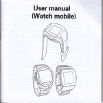
Download RadExPro Plus v. 2011.4 User Manual

RadExPro Plus v. 2011.4
User Manual
(revised 26.01.2012)
DECO Geophysical
Software Company
MSU Science Park,
Leninskie Gory 1-77
119992 Moscow, Russia
Tel. (+7 495) 930 8414
Fax (+7 495) 930 8058
www.radexpro.com
E-mail:
support@radexpro .ru
[email protected]
Table of Contents
Introduction.......................................................................................................................................... 6
System Requirements........................................................................................................................8
Contact Information.......................................................................................................................... 9
Installation.......................................................................................................................................... 10
Working With the Software................................................................................................................ 11
Project Management...........................................................................................................................14
What is a project?............................................................................................................................14
Creating a new project................................................................................................................. 15
Opening an existing project......................................................................................................... 20
Working with Projects........................................................................................................................ 21
Starting work with a project............................................................................................................21
Working with project trees.............................................................................................................. 27
Working with flows.........................................................................................................................37
Flow construction (simple mode)................................................................................................ 38
Complex (graphical) mode of flow creation................................................................................41
Switching between flow editing modes.......................................................................................44
Flow execution.............................................................................................................................44
Logging........................................................................................................................................45
Adding data files to the project....................................................................................................... 48
Adding a data file.........................................................................................................................48
Database Object Selection window - saving and opening project database objects....................... 53
Geometry Spreadsheet - spreadsheet editor for trace header values...............................................58
Using the geometry spreadsheet editor........................................................................................58
Using the editor of mathematic operations with headers.............................................................61
Import of ASCII files................................................................................................................... 61
Trace Enumerator tool................................................................................................................. 68
Import of SPS-X files.................................................................................................................. 69
UKOOA p1-90 files import......................................................................................................... 72
RadExPro header fields...................................................................................................................76
Edit Header Fields....................................................................................................................... 76
Important header fields................................................................................................................ 78
Processing modules............................................................................................................................ 80
Data I/O (Data input/output)........................................................................................................... 80
Trace input................................................................................................................................... 80
Trace Output................................................................................................................................ 81
SEG-Y input.................................................................................................................................82
SEG-Y output...............................................................................................................................86
SEG-D Input ............................................................................................................................... 90
SEG-B Input ............................................................................................................................... 95
SEG-2 Input................................................................................................................................. 96
Text Output ................................................................................................................................. 98
SCS-3 Input..................................................................................................................................99
Super Gather.............................................................................................................................. 101
Data Input.................................................................................................................................. 102
Data output.................................................................................................................................106
RAMAC/GPR ...........................................................................................................................107
LOGIS........................................................................................................................................108
GSSI ..........................................................................................................................................108
2
Geometry/Headers.........................................................................................................................109
Trace Header Math.....................................................................................................................109
Near-Surface Geometry Input....................................................................................................114
Header Averager.........................................................................................................................119
Shift header ...............................................................................................................................120
Header<->Dataset Transfer .......................................................................................................120
Surface-Consistent Calibration*................................................................................................122
Compute Line Length ............................................................................................................... 123
Interactive Tools............................................................................................................................124
Screen Display........................................................................................................................... 124
Plotting*.....................................................................................................................................150
3D Gazer (Display of seismic crossections in real 3D coordinates)..........................................165
Signal Processing.......................................................................................................................... 179
Amplitude Correction................................................................................................................ 179
DC Removal.............................................................................................................................. 181
Bandpass Filtering..................................................................................................................... 181
Butterworth Filtering................................................................................................................. 184
Resample....................................................................................................................................186
Hilbert Transforms.....................................................................................................................186
Trace Math Transforms..............................................................................................................187
Data Enhancement ....................................................................................................................... 189
2D Spatial Filtering....................................................................................................................189
Antenna Ringdown Removal.....................................................................................................191
Radial Trace Transform............................................................................................................. 191
Radon Transforms......................................................................................................................196
Burst Noise Removal ................................................................................................................200
Wave field subtraction............................................................................................................... 201
F-X Deconvolution.................................................................................................................... 210
Spectral whitening..................................................................................................................... 212
Spectral shaping.........................................................................................................................214
F-K Filter .................................................................................................................................. 216
Trace Editing................................................................................................................................. 223
Trace editing.............................................................................................................................. 223
Trace length (Trace length changing)........................................................................................ 225
Trace Math................................................................................................................................. 226
Deconvolution...............................................................................................................................228
Deconvolution (Deterministic deconvolution).......................................................................... 228
Custom Impulse Trace Transforms............................................................................................231
Predictive Deconvolution.......................................................................................................... 234
Surface-Consistent Deconvolution............................................................................................ 235
Nonstationary predictive deconvolution....................................................................................240
Static Corrections..........................................................................................................................246
Calculate Statics.........................................................................................................................246
Apply Statics..............................................................................................................................253
Auto Statics* (Automatic static correction calculation............................................................. 255
Picking (It is old module. We recommend you to use Statics Correction module)................... 264
Auto Statics* (Calculation of automatic statics)........................................................................274
Velocity......................................................................................................................................... 281
Time/Depth Conversion.............................................................................................................281
DB Velocity Interpolation..........................................................................................................285
3
HVA Semblance (Horizon Velocity Analysis Semblance).........................................................286
NMO/NMI................................................................................................................................. 289
HVA (Horizontal Velocity Analysis)..........................................................................................292
Velocity Editor........................................................................................................................... 307
Interactive Velocity Analysis..................................................................................................... 311
Velocity Curve Editor................................................................................................................ 320
Stacking/Ensembles...................................................................................................................... 324
Ensemble Stack..........................................................................................................................324
Migration.......................................................................................................................................326
Stolt F-K Migration................................................................................................................... 326
STOLT3D (3D Stolt F-K Migration).........................................................................................327
T-K Migration............................................................................................................................ 328
VSP............................................................................................................................................... 330
VSP Migration .......................................................................................................................... 330
Curved Profile VSP Migration ..................................................................................................330
2D-3D VSP Migration............................................................................................................... 330
3C Orientation............................................................................................................................344
2С Rotation................................................................................................................................346
sym2ort...................................................................................................................................... 347
VSP Geometry* ........................................................................................................................ 348
VSP Data Modeling................................................................................................................... 354
VSP SDC (Vertical Seismic Profiling Spherical Divergence Correction for non-converted
reflected compressional waves).................................................................................................357
Advanced VSP Display..............................................................................................................360
VSP NMO..................................................................................................................................371
QC (quality control)...................................................................................................................... 373
Ensemble QC............................................................................................................................. 373
Correlation function compute.................................................................................................... 377
Compute fold............................................................................................................................. 379
Apparent velocity calculation.................................................................................................... 380
SSAA (Seismic Sequence Attribute Analysis) ..........................................................................381
CrossPlot (Tied crossplots)........................................................................................................385
ЗС Processing (multi-component processing).............................................................................. 416
Asymptotic CCP Binning.......................................................................................................... 416
Modeling....................................................................................................................................... 420
Hodograph................................................................................................................................. 420
Auto Picking .................................................................................................................................423
First Breaks Picking...................................................................................................................423
Marine........................................................................................................................................... 424
Zero-Offset DeMultiple............................................................................................................. 424
Tides Import*.............................................................................................................................429
Marine Geometry Input ............................................................................................................ 431
Deghosting* (Ghost wave suppression on near offsets)............................................................435
Interpolation.................................................................................................................................. 436
Profile Interpolation* (Interpolation of profile data on a regular grid)..................................... 436
CCP-CMP X Interpolation.........................................................................................................442
Refraction......................................................................................................................................444
Travel Time Inversion* .............................................................................................................444
Easy Refraction* (Processing of seismic refraction data)......................................................... 461
Surface Wave Analysis..................................................................................................................477
4
MASW (Multichannel Analysis of Surface Waves).................................................................. 477
Special tools .....................................................................................................................................504
Map............................................................................................................................................... 504
The menu and tool bar............................................................................................................... 504
Status Bar...................................................................................................................................511
Keyboard and commands...........................................................................................................511
3D CDP Binning........................................................................................................................... 513
Working in binning mode ......................................................................................................... 515
Toolbar....................................................................................................................................... 516
Sequence of work with the application......................................................................................517
Tape Loader (program of reading data from tapes).......................................................................518
System requirements..................................................................................................................518
Working with the program.........................................................................................................518
Well loading and displaying in the RadExPro package................................................................ 521
Wells loading to database...........................................................................................................521
Well displaying.......................................................................................................................... 525
File formats................................................................................................................................528
Refraction mode............................................................................................................................... 530
Development tools - Creation of your own module......................................................................... 531
Microsoft Visual C++ Custom AppWizard...................................................................................531
FUNCTIONS................................................................................................................................ 533
5
Introduction
The RadExPro software is dedicated to comprehensive processing and interpretation of mainly
near-surface on-shore and off-shore 2D seismic, VSP and GPR data, as well as to 2D/3D field
Quality Control (QC).
The software operates on standard Windows-driven PCs and does not make any distinctive demands
on specific hardware or require any additional software.
The scope of the system includes:
Processing and interpretation of 2D on-shore and marine seismic data.
Field QC of 2D/3D seismic data.
Refraction seismic data processing and interpretation.
MASW
VSP data processing.
GPR data processing and interpretation.
The RadExPro is available in several configurations united by a common user-friendly graphic
interface but different in the set of embedded processing modules:
Basic - basic processing of near-surface reflection, refraction seismic data processing, analysis
of surface waves (MASW) ;
Standard - basic processing of near-surface reflection, refraction seismic data processing,
analysis of surface waves (MASW), vertical seismic profile (VSP) data processing;
6
QC - field processing and QC of 2D/3D seismic data, advanced processing of near-surface
reflection data, processing of refraction seismic data, analysis of surface waves (MASW);
Advanced - field processing and QC of 2D/3D seismic data, advanced processing of nearsurface reflection data, processing of refraction seismic data, analysis of surface waves (MASW),
processing of VSP data.
This manual describes the RadExPro Advanced configuration. If you have one of the other
configurations of the software, be aware that some features described in this manual are not present
in your configuration. You can check the content of different configurations on our Web-site:
http://www.radexpro.com
7
System Requirements
Minimum:
Pentium4 CPU
256 Mb RAM
OS MS Windows 98/Me/NT4/2000/XP/Vista
SVGA monitor
Recommended minimum:
Intel Core 2 Duo CPU
1 Gb RAM
OS MS Windows XP/2000/Vista/7
1280x1024 monitor
8
Contact Information
Any questions and requests regarding functions of the software may be addressed to the DECO
Geophysical Software Company:
DECO Geophysical SC
Moscow State Univeristy Science Park
Leninskie Gory 1-77
119992 Moscow
Russia
Tel.(+7 495) 930 84 14
Fax.( +7 495) 930 80 58
Internet: www.radexpro.com
E-mail: [email protected]
9
Installation
Run the software installation executable file and follow the instructions of the Installation Wizard.
10
Working With the Software
There are two ways to launch RadExPro:
From the Start Menu. The program is located in the All Programs menu in DECO Geophysical
group.
From "Windows Explorer", "My Computer", or any other file manager, navigate to the
directory where the program has been installed and launch the file starter.exe.
Before the program is launched the following window will appear:
The window contains a list of already registered RadExPro projects and project management
buttons.
New project... allows creation of a new, empty project, the name of which will appear in the
list of registered projects (Registered projects)
Select project... allows adding an already existing project into the list of registered projects
(Registered projects)
Remove from list button removes the selected project from the registered projects list
(Registered projects)
11
Save list... button saves the list of registered projects into the text file.
Load list... button loads the list of registered projects from a text file.
When required project is selected, click the OK button. To leave without saving changes, click
Cancel.
12
Project Management
What is a project?
All data processing should be performed within the framework of a processing project. A project is
a set of different types of data, their geometry, as well as processing flows applied to the data. Each
project is kept in a separate directory on a hard disk.
A RadExPro project represents a database, divided into Area, Line, and Flow. Area consists of one
or more lines, each line, in turn, is made up of flows.
The objects of a project’s data can contain seismic data, borehole data (wells), time picks (picks),
velocity picks, grids and bitmap images. Each data object of the project is associated with this or
that level of the database, attached to a specific area, or a specific line, or a specific flow. Although
RadExPro provides for working with external data files, in most cases work with a data file should
start from registration in the project database.
For example, you perform the processing of the data, acquired near illage along 3 lines. You may
create a new project (see the section “Creation of new project”), add an area “Unnamed”, and
inside the area you can create 3 lines: “Profile1”, ”Profile2”, and “Profile3” (see the chapter
“Working with a project”, in the paragraph “Working with a project tree”).
Next, you have to load data into the project. In the given case the data represent the set of field
seismograms for each line (the data loading is examined in the chapter “Working with a project”, in
the paragraph “Registration of the data files in the project”). Seismograms of the 1st line should be
tied to the level “Profile1”, the 2nd line tied to the level “Profile2” etc.
13
After loading the data, you may create several processing flows for each line (see the chapter
“Working with a project”, in the paragraph “Working with flows”) and run the tasks.
You may need to save intermediate processing results. You can do this by creating new datasets
inside the project, linked to any level of a project.
You may exit the program and during the next run you can open a project created earlier with area,
lines, and attached seismograms and processing flows (see the paragraph “Opening an existing
project”). You can modify the project, add new lines or flows, change the parameters of procedures
in the flows created earlier etc. All your work is well organized and stored in one place. You can
look through the project to find out what had been done earlier and add something if you need to do
so. After you have finished the processing, you may need to extract the processing results from the
RadExPro project and save them as a file to a disk in one of the standard formats. There are special
modules for data output to external files (see the chapter “processing modules”, in the paragraph
“Data I/O”).
Creating a new project
The process of new project creation starts with determination of a directory on disk, where all data
objects of the project as well as its database files will be stored.
In the RadExPro Project Manager select a New project... button. A dialog window for project
folder selection will appear.
14
Select a directory and click the OK button. If the OK button is not active, it means that the selected
folder already contains another RadExPro project.
After the directory for a new project has been selected the New database window will appear. Enter
the name of the new project in the Title field. If the Create subfolder option is activated, the
subdirectory with the name specified in the Title field will be created in the selected directory.
Otherwise, a new project will be created directly in the selected directory.
After all parameters have been specified, click the OK button. A new project will be created in the
specified directory. In this case the RadExPro program will create five project database files in the
directory:
data.fbl
struct.fbl
15
data.fsp
struct.fsp
atoms.tbl
The name of a new project will appear in the registered project list (Registered projects) of the
RadExPro Project Manager window.
Select the created project by clicking the left mouse button (MB1) (in this case, in the Project
directory field the information about the project path will be displayed) and click the OK button.
Opening an existing project
In order to open a project it should first be added to the registered project list (Registered projects)
in the RadExPro Project Manager window.
If the required project is already on the list, you can simply select it with the left mouse button
(MB1) (in this case, in the Project directory field the information about project path will be
displayed) and click the OK button.
If the project already exists on the hard disk but its name is not displayed in the registered project
list, select the Select project... button. The window for project directory selection will open.
16
Select the directory in which the project is stored and click the OK button. If the OK button is not
active, then it means that the directory selected does not contain a RadExPro project.
If the project directory was successfully selected then its name will appear in the registered project
list (Registered projects). After this, the project can be opened as described at the beginning of the
chapter.
17
Working with Projects
Starting work with a project
After a new project has been created (or an existing project has been opened) the main application
window containing a graphical view of the active project tree will be displayed. If the project is a
new one the window will be similar to the following:
The menu contains the following commands:
Help command launches the RadExPro program help
Options command opens the submenu containing the following commands:
Refraction mode This command switches on and off the specialized mode designed for
processing of the refraction data. When this mode is on, the program respond differently to mouse
18
commands (see Refraction mode part of this manual for details).
Font.... When selecting this command the dialog box for parameters selection for the font to be
used for database element names will open
Logs... When selecting this command, the dialog for logging parameters will open.
Database command opens the submenu containing a number of commands for working with a
project database: Save saves to the active database on disk into a special file with *.dbs extension
Load loads the previously saved database from the *.dbs-file
Add data file adds a new seismic data file to the project
Geometry Spreadsheet allows you to view and edit the trace header field values
Database Visualization launches the Database Visualization application
Database Manager launches the Database Manager application
Database History... shows the processing history of one or another seismic data file registered in
the project
DXF export
This menu entry allows saving horizon picks into the DXF format for further processing in GIS and
CAD systems. When the option is selected the following dialog appears:
19
On the left there is a representation of the project tree with picks. On the right there is a
representation of the resulting DXF file structure, possibly including layers and picks to be exported.
You can add picks to the DXF from the project either using the Add button or double-clicking the
pick name. You can remove picks from the DXF by either using the Remove button, or through a
context menu (right click on the pick name and select Delete... in the pop-up menu).
In the DXF you can create layers and save picks either to the root or/and to these layers. To create a
layer right-click the DXF structure field and select the New layer... command of the pop-up menu.
When created, the layer can be renamed: double-click it and type a new name.
When you are ready with populating the DXF structure with layers and picks, click the Save... or
the Ok and specify the name of the output file. If the Ok button was used the dialog will close,
while using the Save... button allows creating several DXF files within one session.
Coordinates. The two matching headers of the pick are interpreted as X and Y coordinates of the
DXF accordingly, while the pick value is considered as Z coordinate. In case both headers are the
same (e.g. CDP_X:CDP_X), the pick is considered as 2D. In this case, the header value is stored as
X coordinate of the DXF while Y coordinate is assigned 0.
20
Below there is an example of the RadExPro Plus picks exported to DXF and loaded to AutoCAD:
Edit header fields allows you to edit header fields, i.e. delete/change the existing fields and add
new ones
Database Management opens the submenu with two commands: Fix data file location and Bulk
data file location. The first command allows you to change the paths to the source data within the
database and the second command allows you to change the path to the directory containing all
project files. The application of these commands may be required when loading a previously saved
database structure from the *.dbs-file
Tools command opens a submenu containing the following commands:
21
View Map launches the Map application
Velocity model editor launches the Velocity model editor application
Velocity Picks To CMP Matching launches the Velocity Picks To CMP Matching application
Export To Half-Link exports the project database into Geoshare Half-Link data interchange
format
Import From Half-Link imports the project database from Geoshare Half-Link data interchange
format
Exit exits the RadExPro program.
Aside from the above, in the bottom right of the window there are three command buttons designed
for project structure editing:
New button creates a new area, line, or flow
Rename button renames the existing area, line, or flow
Trash button removes the existing area, line, or flow
The status bar at the bottom of the working window contains hints for mouse usage:
MB1 DBLClick double clicking the left mouse button (MB1) on the flow name allows you to
edit it;
MB2 single clicking of the right mouse button (MB2) on the area name, line name, or flow name
launches a context menu with available commands;
MB1 clicking and holding the left mouse button (MB1) on a flow name and dragging it to a line
22
name allows copying the flow into this line.
23
Working with project trees
A project tree is a graphical presentation of data organization in the project. All data is divided into
areas, lines, and flows. Every area must include one or more lines and every line, in its turn, must
consist of flows.
When selecting an existing project, in the main RadExPro window. the project tree with areas,
projects, and flows will open. This tree can be edited. The names at every level are sorted
alphabetically. The window of the already existing project may have the following view:
When creating a new project, a project tree should be constructed. The tree core is a yellow
circle in the upper left corner of the working window.
24
The tree construction order is the following:
Create a new area. There are two ways to do this:
Place the mouse cursor on the yellow circle. Click the right mouse button (MB2) and select the
Create new area command in the context menu. Then, in the opened window enter a name for the
new area and click the OK button.
Place the mouse cursor on the New icon, click the left mouse button (MB1) and, holding it down,
drag the icon to the yellow circle and then release the button. In the opened window enter a name for
the new area and click the OK button.
Create a new line inside the area. There are two ways to do this:
Place the mouse cursor on the area name, click the right mouse button (MB2) and select the Create
line command in the context menu. Then, in the opened window enter a name for the new line and
click the OK button.
Place the mouse cursor on the New icon, click the left mouse button (MB1) and, holding it down,
drag the icon to the area name and then release the button. In the window that has opened enter the
name of a new line and click the OK button.
A new flow is created inside the line. There are two ways to do thCreate a new flow. There are
two ways to do this.
Create a new flow. There are two ways to do this:
Place the mouse cursor on the line name, click the right mouse button (MB2) and select the
Create flow command in the context menu.
Place the mouse cursor on the New icon, click the left mouse button (MB1) and, holding it down,
25
move the cursor to the line name and then release the button. In the window that has opened enter
the name of a new flow and click the OK button.
Similarly, areas, lines, and flows can be added to the tree of an already existing project. If
necessary, any tree element (area, line, or flow) can be renamed or removed.
In order to rename a tree element, move your cursor over it, click the left mouse button (MB1), drag
it to the Rename icon, and release. Enter a new name for the element in the window that has
opened and click the OK button.
In order to remove the tree element, move your cursor over it, click the left mouse button (MB1),
drag it to the Trash icon, and release. Confirm the removal in the opened window.
ATTENTION: The tree element removal cannot be undone!
When the first flow is created in the profile, a “-” sign appears to the right of the profile name.
Clicking this sign collapses all flows in that profile into a single line:
26
Clicking the “+” sign expands the list of flows. This makes it easier to navigate projects containing a
large number of profiles and flows. When all flows in all profiles are collapsed, the project looks as
follows:
When identical processing procedures are to be repeated for each line, profile copying can make
working with the project considerably easier.
To copy a profile, click and drag it with the left mouse button to the area name. The new profile
name selection dialog box will appear.
27
28
Enter the new name and press OK. The profile will be copied with all processing flows and parameters.
29
Attention: when profiles are copied, all parameters, including all input and output data (data sets, picks
etc), remain unchanged. Don’t forget to change the names of input and output files and data sets before
running the new flows.
Project navigation
The project can be scrolled up and down using the vertical scrollbar or the mouse wheel.
Queues
Flow execution can be queued. Both individual flows and entire profiles (i.e. all profile flows one
after another) can be added to an execution queue.
To add a flow to a queue, right-click the flow, select the Add to queue menu item, and then select
30
the number of the queue to which the flow will be added:
The program allows running flows in four independent queues. Queues are launched in parallel; this
reduces the total processing time on multi-processor or multi-core machines.
After the queue number is selected, the queue window will appear:
The upper part of the window contains tabs that allow switching between the queues.
The current queue editing window shows the list of active flows added to the queue and their status. The
flow status indicates the flow processing stage:
Not started – the flow has not yet been started;
Running – the flow is running;
Canceled – execution of the flow has been canceled.
The flows in the queue are executed one after another, from top to bottom. The flow execution order
can be changed:
31
–
–
move the flow up one level in the queue.
move the flow down one level in the queue.
The right part of the window contains buttons used to manage the list and the flow procedures:
Delete – delete the selected flow from the queue
Delete all – delete all flows from the queue
Run this queue... – run the current queue
Run all queues... – run all queues
Stop this queue – stop the execution of the current queue. This button is active only when the
queue is running.
Show status – opens a window showing the current status of all queues:
Here:
Queue – queue number
Batches – number of the process in the queue
Status – current process execution status
Always on top – if this option is enabled, the queue window will always be displayed on top of
other program windows.
An example of queues is shown below. Two queues were created; each of them contains a set of
flows in separate profiles. When all queues are launched, the two current queues will be run in
parallel.
32
33
Working with flows
Data processing and visualization is performed by creation of execution sequences (flows) from the
set of available modules. These flows are stored inside the database and can be changed, copied, or
removed.
Such organization has a number of advantages because it allows storage of the processing history,
which in turn allows you to return to any step and repeat the whole process, with different
parameters or reuse the already created processing flow with another data set.
The processing sequence (flow) is a set of processing modules, whose inputs and outputs are
somehow connected.
RadExPro has two modes of flow presentation: simple (text) mode and complex (graphical) mode.
In the simple (text) mode the processing flow is represented as a list of processing modules so that
the output of every module is connected to the input of the module that follows it. The flow is
conducted sequentially (top-down) and linearly.
In the complex (graphical) mode the processing modules are presented as icons and the links
between them as tubes. The inputs and outputs of the processing modules are manually connected
by tubes. The modules can have several inputs and outputs. The processing flow can branch out and
form cycles. Such presentation of the flow gives more flexibility in data processing organization.
Owing to this, the flows created in graphical mode cannot always be presented in graphical mode.
Every flow starts with one of the modules of data input from the Data I/O chapter. Usually (for files
registered in the project) it is Trace Input. A data input module initializes the flow and allows
selection of data for processing. There could be several data input modules within one flow. This
can be useful, for example, for:
combining several data sets for co-processing;
data set processing by different methods with succeeding co-visualization by Screen Display
34
module or combining in one output file.
There are also modules designed for data editing and processing: amplitude correction, filtering,
stacking, etc. Every flow usually ends with a data output module, saving processing results on harddisk (for instance, Data/Trace Output) and/or by interactive tools (for instance, Screen Display).
The result of every processing routine/module can be adjusted by changing the parameters of the
module.
Flow construction (simple mode)
When you double-click the left mouse button (MB1) on the flow name in the project tree, the flow
working window will open. If simple (text) representation of the flow is possible, then by default
the flow will open in simple mode. The window is divided into two parts: the right one is a list of
available routines (modules) which can be used to create a flow; in the left part the flow itself, i.e.
the modules used in the active flow, are displayed.
35
The flow allows you to conduct various manipulations with the seismic data registered in the project
(for example, processing, correction, interactive analysis). Manipulation of external files is also
possible.
The modules from the right part are grouped by chapters. For example, Data I/O (data input/output),
Signal Processing, Interactive Tools, etc.
You can include a module into the active flow by two methods:
Click the left mouse button (MB1) on the name of the desired module in the list of available
routines in the right part of the window and, holding it down, drag the mouse cursor to the left part
of the window and release the button (drag-and-drop).
Double-click the left mouse button (MB1) on the left side of the working window and select the
required module from the list of available routines that will open as a pop-up menu;
When a module is being added into the flow, a dialog box with the module parameters will appear.
The way it looks depends on the module selected.
When creating a flow the following operations are possible:
Switching module state in the flow (active/inactive) - is performed by clicking the right mouse
button (MB2) on the name of the module in the flow. Inactive modules will be displayed in narrow
italics, and three * (***) will appear before its name
Transfer of a module in the flow - is done by clicking the left mouse button (MB1) on the
module name and, holding it down, moving the cursor to a new position and releasing the button
Viewing and editing of module parameters - is performed in a special dialog window that
opens when you double-click the left mouse button (MB1) on the module name in the flow
Module duplication - is done by means of the keyboard combination Ctrl+MB 1 on the module
36
name
Module removal - is done by double-clicking the right mouse button (MB2) on the module
name while simultaneously holding the Ctrl. key down. When doing this, the module with set
parameters will be removed from the flow and placed onto the clipboard
Restoring the last removed module from the clipboard - is done by means of the keyboard
combination Shift+MB1 in the flow construction window. The removed module can be restored not
only in its initial flow but also in any other flow of this project
In the working window menu the Help, Options, Database, Tools elements are the same as in the
main window of the program (see How to Start). The Exit command of the menu, unlike the similar
command in the main window, does not result in the exiting of the program. The selection of this
command allows closing the flow window and returns the user to the project tree viewing, i.e. to the
main RadExPro window. The menu also contains the following commands specific to the flow
window:
Run launches active flow execution
Flow mode allows the user to specify the mode of memory usage during flow execution.
When selecting this command the following window will be displayed:
37
The All at once (all in memory) mode is set by default. When using this mode all data from the
flow is placed into system memory. This mode is used for small data files. For large data files the
Framed mode is used. When using this mode all data from the flow is processed in portions, their
volume in traces is defined in the Frame width (traces) window. Activation of the Honor
Ensemble boundaries option avoids trace division inside the ensemble.
Complex (graphical) mode of flow creation
In the graphical mode the left side of the working window contains a graphical presentation of the
flow, and the right side contains the set of available processing modules.
Every module included in the flow is presented as an icon.
Module inputs and outputs are connected manually. The module input is displayed as a small circle
located in the upper part of the icon; the module output is displayed as a small circle located in the
bottom part of the icon. When the mouse cursor is placed on the icon a small hint with the module
name will appear on the screen.
In the case when several tubes are connected to the module input, all data from these tubes will be
combined (in order of tube creation). In the case when several tubes are connected to module
output, all data "out-flowing" from the module will be distributed to every tube.
Creation of the flow in graphical mode comprises modules adding to the flow and connecting them
by tubes. Later the modules can be added to the flow, temporarily excluded from it, copied onto the
clipboard and/or pasted from it.
38
To add a module into the flow, drag it from the list or double-click on the left side of the flow
window and select the desired module from the pop-up menu.
To connect the input of one module to the output of another, click the right mouse button
(MB2) at the input (or output) of one module and drag the tube that appears to the output (or input)
of another module. When dragging, the line showing the tube will follow the mouse cursor. When
the cursor points to a possible connection site, the tube-line will be thicker. At this moment, you can
establish the connection by releasing the right mouse button. It is impossible to connect input with
another input or output with another output.
To change the parameters of the module already included in the flow, you can simply
double-click the left mouse button (MB1) on the module's icon in the flow, where upon the dialog
box for parameter specification will appear.
To move the module icon, drag it by holding down the left mouse (MB1) button.
39
It is possible to exclude the module from the module sequence under execution but keep it in the
flow (make the module inactive). Inactive modules are slightly faded. To enable switching the
module mode in the flow (active/inactive), click the right mouse button (MB2) on the module's
icon.
To remove the module from the flow, double-click the right mouse button (MB2) on the icon of
the module in the flow while simultaneously pressing the Ctrl. key. The module with set parameters
will be be removed from the flow and placed onto the clipboard.
To remove all tubes connected to the module input or output, click the left mouse button
(MB1) on the corresponding small circle in the upper or bottom part of the icon of the module in the
flow.
To copy the module onto the clipboard, click the left mouse button (MB1) on the center of the
icon while simultaneously pressing the Ctrl. key.
To paste the module from the clipboard, click the left mouse button (MB1) on the left side of
the screen while simultaneously holding down the Shift key.
In the graphical mode the menu of the flow working window contains the same commands as in the
text mode (see Flow construction (simple mode) chapter).
Switching between flow editing modes
When creating a new processing flow (or when opening an already existing flow, if it can be viewed
in text mode) a simple presentation mode is selected by default. To switch to the complex mode,
double-click the right mouse button (MB2) on the left side of the window. The flow will be
converted and presented graphically but the routine's sequence will be the same as in the flow
presented in simple (text) mode.
Simple (text) flow is executed sequentially and linearly. Graphical (complex) mode can have
branches and cycles. In this case a simple (text) presentation of such a flow is impossible and when
opening this flow it will be displayed graphically.
40
If the flow is displayed in graphical mode but it does not have branches and cycles, then it also can
be displayed in a simple (text) mode. To switch this kind of flow into simple mode, double-click the
right mouse button (MB2) on the left side of the window.
Flow execution
The Run command of the working window serves to execute the flow. A small status bar will appear
on the screen. On the status bar the list of active modules of the flow and task completion rate for
every module will be shown.
At present, in the flow there are several interactive modules meant to interact with the user during
their execution (for example, Screen Display, VSP Display, etc.). Interactive modules exist in a
separate window and can be considered by the user as independently executed tasks. Via standard
Windows functions, it is possible to switch from the interactive module back to the RadExPro
working window and continue working with it. At the same time the flow containing the interactive
module is still under execution and the interactive module window is available for visualization and
activation. Thus, more than one flow can be executed. This is a very convenient feature because it
allows you to compare the data on the screen. The interactive modules are completed either through
the module interface or at the completion stage of the whole program (upon closing of the main
working window). In either case the flow is executed to the end. When launching more than one
module at once, remember that every launched flow needs computer memory (mainly for data
storing) and that is why a limited number of flows can be launched at the same time.
It is possible to interrupt flow execution. To do this, close the status bar and click the OK button
when the corresponding question appears. You should use this opportunity only as a last resort
because such interruption is abnormal and may result in loss of system resources (of course they
will be restored after a Windows restart).
Logging
The RadExPro program includes the facility of logging of flow execution. When a flow is being
executed, appearing messages can be written to a text file (log). When necessary, this file can be
viewed by any text editor. It could be helpful to look into the log, when the flow execution
terminated abnormally. The log could explain the reason of the error, or at least define at what stage
41
the problem occurred. The logging facility is optional, i.e. it can be switched off. Logging
parameters can be set through a dedicated dialog window. All logs are stored in the LOGS subfolder
of the root folder of the project. The structure of the LOGS folder repeats that of the project, so the
logs corresponding to a certain flow are stored in the folder of the same name. Each flow execution
creates a new log. The name of the log consists of the date and time of launching of the flow
execution, to distinguish the logs related to one flow that was executed several times. The name
structure of a log is yymmddhhmmss.txt (For example, the name of the log 090101001053.txt
indicates that the flow was executed on the 1st of January, 2009 at 00 hours 10 minutes 53 seconds.)
The Logging parameters dialogue can be opened using the Options->Logs... entry of the main
program menu.
42
The logging parameters:
Enable logging – enables/disables logging facility.
Log content – defines message types to be included into the log:
Status – doubling of the messages from the Status Window
Report – dedicated messages, created specially for logging.
Log size limit - this group combines parameters controlling the size of the LOGS folder:
Track log size – enables/disables log folder size tracing.
Maximum log size – sets maximum log folder size in MBytes
Action on reaching log size limit –defines the action to be performed, when log folder size reaches
maximum. Select one of the following:
Automatically delete old logs
Warn on project loading Adding data files to the project
Though RadExPro provides for the possibility of working with external (in respect to the project)
data files, in most cases any operations with a data file should be started with its registration in a
43
database of the project so that you can use the program's features in full measure.
There are two ways of adding a data file to the project. Having created a RadExPro project, area,
line, and flow, it is possible to have external (in respect to the project) files registered by means of
entering it into a flow via one of the data input routines (for example, SEG-Y Input) and then saving
it in the project via the Trace Output routine. However, in most cases the alternate method is more
convenient. Select the Database menu item in the main RadExPro window (project tree window)
or in the working window of any flow within the project and then select Add data file... in the
submenu that has appeared.
This command activates a special tool for adding data files.
44
Adding data files to the project
Adding a data file
When the Add data file... command of the Database menu is selected, the Data File: dialog box
will appear.
In the Format field, select the format of the file to be registered in the project.
Supported data formats
At present the system is compatible with 7 standard data formats (SEG-Y, SEG-2, SEG-1, Pulse
EKKO, RAMAC/GPR, Zond, Diogen) as well as with User Defined format. The user defined
format support allows reading the data presented in any demultiplexed format with fixed length of
file header and trace header, as well as fixed number presentation and byte order throughout the data.
When selecting one of the standard formats, RadExPro fills in the project database header fields
automatically on the basis of standard data location in the headers of the format selected. If the
format of the source file is not completely compatible with the accepted standard you can apply
format remapping (Remap header values). When selecting a user defined format always apply
remapping to correctly fill in the header fields.
45
Dialog parameters
Format - select a file format form the list of formats
2D Survey, 3D Survey - the switcher that defines file identification in project as 2D or 3D
surveys
Profile - in this field you can define the sequence number of 2D profile if 2D Survey is selected
IBM Floating Point - if this option is activated the amplitudes (trace counts values) will be read
from the file as 32-bit real numbers with a floating point in the IBM Floating point format.
Store headers outside db - if the option is off, the headers of the file under registration will be
stored directly in the project database file. Otherwise a separate file will be created inside the
directory for storing the headers. If there is much data in the project, the storage of headers in
separate files increases program operation speed. This option is activated by default.
Format definition - a group of parameters of the user defined format. These parameters are
available only when selecting the User Defined format from the Format list:
File passport - in this field, define a file header size expressed in bytes (0 - if the file header is
lacking)
Trace passport - in this field, define a file header size (0 - if the file header is lacking)
Data format - in this field, select the format of trace samples in the input file. Possible variants:
I1- 8-byte integer
I2- 16-byte integer
I4 - 32-byte integer
R4 - 32-byte real with floating point
46
UI1 - unsigned 8-byte integer
UI2 - unsigned 16-byte integer
UI4 - unsigned 32-byte integer
If R4 format is selected in the field, the data will be read either as an IBM floating point or as
IEEE, depending on the IBM Floating Point switch status. For any other Data format header the
IMB Floating Point status is disregarded.
Reverse Byte order - if this option is activated, the program will assume that all values in the
file are recorded with reverse byte order
Remap header values - if this option is off, the header fields in the project database will be filled
in automatically on the basis of the standard definition of the selected format. If the option is on, the
header fields will be filled in accordance with format remapping. If the option is active then a text
field for remap specification as well as Save remap... and Load remap... buttons allowing you to
save the active remap in a database and to load the already saved remaps, respectively, via the
Database Object Selection (see Database Object Selection window chapter) become available.
Example of format remapping:
RECNO,4I,,181/ILINE_NO,2I,,189/CDP_X,4R,IBM,197/CDP_Y,4R,IBM,201
In this example:
RECNO = database header field name where the values from the trace header field specified in a
remap will be recorded;
4I = a field format in a trace header, i.e. a format in which the value is stored in the source file,
in this case it is a 32-byte integer.
47
IBM or IEEE — flag, identifying the representation standard used for the real floating pointnumbers. Used for the 4R format only. For the integer types the flag is not used, and nothing is
placed between the two commas.
181 = offset of the required field in the trace header expressed in bytes;
A field format may contain the following maps:
1I - 8-byte integer;
2I - 16-byte integer;
4I - 32-byte integer;
4R - 32-byte floating-point real (either IBM or IEEE standard depending of the flag that follows);
8R – 64-byte floating-point real.
Thus, RECNO,4I,,181 means that RECNO header field corresponding to the receiver point number
will be filled by 32-byte integer values read from trace headers starting with the 181th byte from the
beginning of the trace header.
File - After format and other parameters have been selected, click a File button and select a data file
which should be registered in the project from the file selection window. The number of traces
contained in the file will appear in the Trace count field directly under the button. The trace number
will be computed on the basis of the format and remap selected. If a file is not compatible with the
format selected, then a trace number may be populated incorrectly.
After all parameters and the file name have been defined, click the OK button. A Database Object
Selection (see Database Object Selection window chapter) window will open where the user will
be asked to enter a name under which the data set from the source file (dataset) will be registered in
the database and to select a database level where the data set from the source file will be stored.
We recommend that all seismic data be stored in the database at the Line level. Select one of the
48
database sections of Line level and specify the name for a new data object under which the file will
be registered in the project, and click the OK button. Wait until the selected file is registered in the
database.
The process of registration will display as a progress bar.
49
Database Object Selection window - saving and opening project
database objects
The Database Object Selection window in the RadExPro program is a standard tool for operating
with database objects similar to open/save file dialog box which is a standard tool for manipulation
of files in a Windows OS.
Almost every time you choose any existing RadExPro project database object or when saving a
new object to database you will see the Database Object Selection window. The header of the
Database Object Selection window will contain an enquiry which will depend on the task under
execution.
Below you can see the Database Object Selection window that appears while a new data file is
being registered in the project:
The project tree is shown to the right in the Location field, and the active section is selected. In this
window the user can navigate throughout the database structure choosing the desired section. All
objects of this kind registered in the active DB are displayed In the Objects field to the left. At the
top is the Object name field, in which the name of the selected object is displayed.
In this example the project database contains 2 sections of Area level (area1 and area2), in the
area1 section is one section for Line level (line1), which, in its turn, contains one section for Flow
level, i.e. a flow (some_flow). In the current section there is one data file, work1 that has already
50
been registered. In the Object name field the user is asked to enter a name under which the new file
will be registered in the project.After the name has been selected and the OK button is pressed, the
data will be registered in the current project database section (in this example that would be line1). In
order to register a file in another database section, change the current section.
Similarly, when opening any existing database object, you should first select the DB section,
containing the required object, and then select the object from the list of already existing objects of
this kind in the section. Below, is an example of the Database Object Selection window appearing
while loading the previously saved format remap:
In this example, in the active section of Area level (2D area) there is only one remap of remap ibm
format and this is the remap chosen by the user for loading.
The Database Object Selection window is used in different RadExPro program modules for
opening/saving of different types of data objects. Therefore, in the Objects field, only the objects to
which the current operation can be applied are shown. Thus, when selecting a file with a seismic
dataset registered in the project, only the datasets that belong to the active level will be shown in the
Objects field. Objects of another type (for example, picks) belonging to the same database level will
not be displayed.
You will also see two buttons in the Database Object Selection window:
Rename - is used to change the name of the selected object. To do this, select the desired object in
the Objects list, enter a new name in the Object name field, and click the Rename button. After the
51
operation has been confirmed by the user, the name of the selected object will be replaced by the
new one.Delete - is used to delete the object from the database. To do this, select the desired object
from the Objects list and click the Delete button. After the operation has been confirmed by the user
the object will be deleted from the project database.
ATTENTION: if the selected object is a set of seismic data, only the file registration in the project
will be canceled, but the file will remain on disk. Objects of any other type are stored directly in the
project database and if they are deleted from the database they are also deleted physically. This
operation cannot be canceled or undone!
52
Geometry Spreadsheet - spreadsheet editor for trace header values
The Geometry Spreadsheet application is meant for spreadsheet visualization of header field values
of a data set in the project and for performing operations with them.
To launch the application, select a Database/Geometry spreadsheet command either from the main
program window (project tree window) or from the working window of a flow. After a data set has
been chosen in the Database Object Selection dialog box that appears, the Geometry spreadsheet
application window will open. The window will contain one column with TRCENO header field
values (trace numbers) for a selected data set.
Using the geometry spreadsheet editor
The Geometry spreadsheet editor menu includes the following options:
Fields - opens the commands list, that allows you to add and remove columns from the table.
Add field – adds one or several columns to the table with the values of chosen fields. The choice
of header fields is performed in the pop-up window.
53
In order to choose several header fields, select them with the mouse, holding the Shift or Ctrl
button. The buttons Save template selection and Load Template selection allow you to save the
chosen headers set as a template in the database and load the templates that have been saved earlier.
Hide field – hides the selected column from the table.
Edit – opens the list of the following commands.
Save changes – saves all changes to the fields carried out during the work of the application.
Undo all changes – cancels all the changes.
Tools – opens the commands list, that allows different operations with headers, import/export of
the data.
Header Math – performs mathematical operations with the header values (see the paragraph
“Using the mathematic operations headers editor”)
Export...—exports the content of the spreadsheet to a file in ASCII format
Import... – imports the file in ASCII format. You should specify the text rows and columns to
import into the spreadsheet (see the paragraph “Import of files in ASCII format”).
Import SPS X...—allows import of the data to the header fields from the SPS-X files (see the
paragraph “Import of SPS-X files”).
Import UKOOA p1-90... allows import of UKOOA p1-90 files
Trace Enumerator – invokes the tool for the specification of continuous trace numbering, sorted
by two header fields (see the paragraph “Trace Enumerator tool”)
Exit – leads to exit from the geometry table. If there are some changes to the header fields
during the work, there will be a saving request.
54
The following buttons and keys are used during the editing of the spreadsheet:
Single left mouse button click (MB1) on a header column selects the whole column. In order to
select several columns, select them one by one, holding the Ctrl button (Ctrl+MB1).
Double left mouse button click (MB1) on a header column sorts the values in the column in
ascending order
Double left mouse button click (MB1) on a cell allows text editing
Single left mouse button click (MB1) on
a cell selects the cell; use the left mouse button
holding the Shift (Shift+MB1) in order to select the values set in the column or several columns.
The selected values set can be copied to the clipboard using the Ctrl+C buttons.
Select the cells and use the buttons Ctrl+V to insert the values from the clipboard into the cells.
If the cells’ size in the clipboard exceeds the selected block that you are going to paste, only a part
of the values from the clipboard will be inserted.
Ctrl-PageUp: jumps to the start of a column
Ctrl-PageDown: jumps to the end of a column
Ins: fills in the selected block with new values. You should enter the start value
in the field From, while the increment is entered in the field Step.
F: finds the given value in the current column.
55
Using the editor of mathematic operations with headers
The module Trace Header Math, designed for mathematical operations with header values, is
activated using the command of the geometry table editor window Tools/Header Math…
The module description is given in the paragraph “Processing modules” → “Geometry/Headers”
→ “Trace Header Math” of the present manual. The single distinction is that in this module the
mathematical operations are applied to the headers in the table immediately after you click the OK
button in the module's parameters window.
Import of ASCII files
When the Tools/Import command is selected from the menu of the Geometry Spreadsheet
window the Import headers dialog box appears:
56
Import parameters
The column corresponds to the specified matching field
Content of the selected ASCII table file
File... - opens a standard window for ASCII spreadsheet file selection from which the values
will be imported
Matching Fields - shows the header field for which existing values will be compared to the
values of the column selected for this field, while importing the columns selected in the Assign
Fields field into corresponding header fields
Assign Fields - shows the name of the headers to which the values imported from the columns
will be assigned.
The Matching Fields and Assign Fields correlation is shown in the following example: if you
set the parameters the way it is shown in the Figure above, then in all traces with a field value
RECNO equal to 40 the REC X field values will be replaced by 413291.0. In traces with a field
value RECNO equal to 41 the REC_Х field values will be replaced by 413289.0, etc., i.e. the
57
settings in the Matching Fields field set a fitting criterion. When fulfilling this fitting criterion the
import is accomplished according to the Assign Fields field settings.
Both the Matching Fields and Assign Fields fields have the following buttons:
Add... - this button adds a header name from the headers list in the field
Delete - this button deletes a header name from the field
Individually for every header in the lists of Matching Fields and Assign Fields fields the
following parameters can be set
Column - in this field a column number is shown in a text file which, at this moment, is
correlated with a selected header. To change the conformity of headers and columns: (1) select a
desired header, (2) click the left mouse button (MB1) on the column that should be correlated with
this header and (3) click the Column button. In the Column field a new column number will
appear. Also the value in the field can be changed manually
Multiplier - the data from the selected column will be multiplied by this value while
correlating with values of the selected header (in Matching Fields case) or while importing into
the selected header (in Assign Fields case).
There is also a group of parameters Lines where the range of the lines in the text file should be
defined. In accordance with the Matching Fields and Assign Fields fields settings the values
imported will be accomplished only from the lines of the selected range. To set a number for the
initial line of the range click the left mouse button (MB1) on the desired line in the text file content
window and then click the From button. The selected line's number will appear in the From field.
Similarly, a finite line's number can be specified in the To field via the To button. Also, the lines'
numbers can be specified in the corresponding fields manually (the numerations of lines in a file
starts with 0).
The Save template and Load template buttons are designed to save current import parameters in
a template of the project database and to load import parameters from a previously saved template
58
respectively.
Load with interpolation option allows to import file with interpolation. In case of presence
missing values in any part of the file – they will be linear interpolated by the header field which is
set in Matching field block. To set the header – choose it in the Reference field option. By pressing
OK button the following message will appear:
Cancel – procedure of importing values to headers will be canceled with returning to
Import Headers window. By pressing Yes button the value, which is currently displayed on
dialog box, will be interpolated. Yes to all — all missing values will be interpolated.
Extrapolate - extrapolates values, missing at the beginning or in the end of file:
No extrapolate – extrapolation will not be done;
59
Use edge values – missing values will be filled equal the last value which is present in the
file
Extrapolate – extrapolation using specified trend. Trend will be calculated by number of
points, selected in Points to estimate trend field.
Recommended procedure:
First, click the File... button to select an ASCII spreadsheet file from which the values will be
imported. File content will be displayed in the Import headers dialog box.
Then, specify the line range from which the values will be imported. To do this, select the first
line to be imported by clicking the left mouse button and then click the From button in the Lines
group. The number of the line which will be imported first will be displayed in the From field. Click
the left mouse button on the last line you would like to import and click the To button in the Lines
group. The number of the last imported line will be displayed in the To field. (Use a scroll bar while
selection if necessary). Also, the lines' numbers can be specified in the corresponding fields manually
(the numeration of lines in a file starts with 0). Line range specification is compulsory even when all
lines from the file are imported!
Use Add... button to select the headers from the list of the headers for the Assign fields and
Matching fields fields.
Correlate selected headers with columns in the file. To do this, click the left mouse button (MB1)
on the header name in the Assign fields and Matching fields fields, then click on the column with
displayed text that corresponds to the selected header. After that, click the Column button and the
column number will appear in the Column field. Set Multiplier value for the selected header.
When all parameters are set, click the OK button. Values import will be accomplished. The
header field values, where the values have been imported to (i.e. fields from the Assign fields list),
will appear as separate columns in the Geometry Spreadsheet window.
In case of missing values in the file in any column, warning message with the position will
appear. Press Cancel to stop importing process and return to Import headers window. While
60
pressing Skip button current value will be skipped without changing in the header (if Load with
interpolation function is disabled). Press Skip all button to skip all missing values in file (if Load
with interpolation function is disabled).
Trace Enumerator tool
A tool dialog box appears when you choose the command Tools/Trace Enumerator from the
menu. This dialog box allows you to sort traces by two header fields and then to assign a continuous
numbering index to them, the values of which are entered in the third header field.
61
62
Primary key (header field that will be used as a primary sort key) and Secondary key (header field
that will be used as a secondary sort key) are set in the Sorting field.
The progression parameters for continuous numbering—Value and Increment—are set in the field
Progression where you choose the field to which the acquired values will be written—Target
header field.
Example of usage:
For instance, if the data include two traces with one FFID value, differing by TRACENO values,
after using the Tool with parameters which are represented on the figure, the values of the field
CHAN can be:
FFID TRACENO CHAN
1
1
0
1
2
1
2
1
3
2
2
4
Import of SPS-X files
To import SPS-X files use the menu command Tools/Import SPS-X.
The following dialog import window will open:
63
Recommended procedure:
Choose the SPS-X file using the File…button. The file content will be reflected in the lower part
of the window.
Please indicate the lines of the file to load with the number of the starting line in the From field
and the number of the ending line in the To field within the Lines section of the parameters. You
can also position the mouse cursor on the required line and click the From or To button—the line
number will be automatically reflected in the corresponding field.
Choose the mode of line separation into separate fields Text table type
Delimited by columns: the fields in line will be separated by a space.
Fixed width by positions: the fields in line will have a distinct position relative to the start of the
line and a fixed width.
Set matching between the columns (positions) in file and header fields to which the data are
loaded.
64
The matching is carried out by the fields Field record number and Chanel. The loading is performed
to the Source line, Receiver line, Source station location, and Receiver station location.
First of all, when you load a line you can determine the Field record number, corresponding to the
line. Then, the channel numbers are determined for this record number using the fields From
chanel, To chanel, and Chanel increment. Furthermore, the values are loaded to the indicated
headers for each trace from the fields Source line, Source station location, Receiver line (pairs
record number - chanel), described by the given line.
As well, the value of Receiver station location is loaded for each trace according to the fields First
receiver station location, Last receiver station location, and Receiver station location increment.
You should set the name of a specific trace header for each field that matches.
The current header names for each field (column Description of Field in the list of the upper left
part of the window) are visualized in the right part of the list (Header Name column). To change
the header corresponding to any field, double click on its name with the left mouse button or use the
Change header button.
In order to set the column (position) in the file corresponding to a field:
Select the field in the list using the mouse.
In delimited mode, indicate the column number or point the mouse cursor to the required
column and click the Set column button.
In fixed width mode indicate the values of the first and last position in the corresponding entry
fields, or select the required range using the mouse and click the Set pos button. The current range
will be visualized in red, while the range being edited is visualized in blue (their intersection will be
viewed in green). The fields Chanel increment and Receiver station location increment can be filled
in by two methods: from the file (From file), indicating the column (positions), or manually
(Manual), setting the value in the corresponding entry field. After setting all the parameters, click
the OK button to load data from the SPS-X file.
65
UKOOA p1-90 files import
UKOOA p1-90 files are imported using the Import UKOOA p1-90 menu command.
The program imports source and receiver coordinates and elevations from the UKOOA file; the rest
of the information contained in the file is ignored. Search for the values corresponding to sources
and receivers is performed based on the S and R identifiers (source and receiver identifier,
respectively) located at the beginning of the line in the file.
The import dialog box looks as follows:
66
The dialog box is divided into two main areas that control the import of headers associated with
sources and receivers: Source format definition and Receiver format definition, respectively.
Each import block has four columns: Field description – header field description, Beg – beginning
of the column corresponding to the header value in the file being loaded, End – end of the column
corresponding to the header value in the file being loaded, and Header name – header field name.
Header fields to which other values are linked are shown in blue. For source coordinates this is the
FFID (shot number) field, for receiver coordinates – the CHAN (channel number) field. Three
repeating CHAN header, coordinate and elevation fields are specified for receivers in the geometry
assignment
block
since
the
standard
UKOAA
p1-90
file
has
three
columns
for
coordinates/elevations. By default the range of values for each of the headers is specified in
accordance with the standard UKOOA p1-90 file format (format description can be found at
www.seg.org,
the
following
link
is
active
67
as
of
September
1,
2011:
www.seg.org/documents/10161/77915/ukooa_p1_90.pdf ).
Recommended procedure:
To load the file, press the File... button and select the file you need. Its contents will be displayed in
the lower pane of the dialog box:
Left-clicking a line that contains a header field highlights the corresponding value column
68
(according to the standard file format). If columns with header values are invalid for some reason,
they need to be redefined. To do this, select the relevant header in the Source format definition
block, select the range of values corresponding to that header in the lower pane by clicking and
holding the left mouse button, and press Set pos. Values in the Receiver format definition block
are assigned in a similar manner. The Load template... and Save Template buttons allow saving
and loading the current file import settings. The Load default button restores default UKOOA p190 file import settings according to the current format.
Make sure that values correspond to all headers are valid and press OK. The coordinate and
elevation values will be written to the specified headers in the database.
69
RadExPro header fields
To store auxiliary information on seismic data, the RadExPro program uses its own set of header
fields. They are kept in database files, separate from data files which provides fast access to the
header fields.
When creating a new project the set of header fields in the project is similar to trace headers in SEGY format. However further the header fields can be edited, i.e. you can add new fields and delete
and rename the existing ones. To view and edit the active set of project header fields you should
select the menu command Database/Edit header fields... in the main window of the program
(project tree window).
In the new (or existing) header fields you can record various information. For example, seismic trace
static shift or arrival time picked on the trace. You can do mathematical operations with header field
values, convert them into picks, display changes of header values in different datasets, etc.
Edit Header Fields
To view and edit an active set of project header fields, select the menu command Database/Edit
header... from the main window of the program (project tree window).
The window containing the list of headers from the active project will open:
70
In the header list there are three fields:
Name: the name of header field
Type: the type of header field value
Description: header description
To add a new header field, click the Insert button. To edit the existing header field, double-click the
left mouse button (MB1) on the name of the required field. To delete an existing header, select it in
the list with the left mouse button (MB1) and click the Delete button. After the deletion has been
confirmed the field will be deleted from the project.
When adding a new header field or editing the existing one, the following dialog box will appear:
Here you can specify/change the name, format, and description of the header. Enter/change the
header field name in the Name field.
Select the required format of the header from the list of available formats. The header field values
can be stored in one of the following formats:
Integer, Int32: 32-byte integer
Int8: 8-byte integer
Int16: 16-byte integer
71
Real: 32-byte real with floating point
Real8: 64-byte real with floating point
In the Description field, specify the annotation or textual description of the header field.
After all parameters have been set, click the OK button. To exit without saving the changes click the
Cancel button.
Important header fields
Below you can find a list of some most important standard RadExPro header fields. We advise you
not to delete these fields or change their meaning.
DT: sampling interval in ms
NUMSMP: number of samples per trace
FFID: seismogram number (shooting number)
SOURCE: source point number
CDP: CDP number
RECNO: receiver point number
SOU_X, SOU_Y: X coordinate of the source, Y coordinate of the source
REC_X, REC_Y: X coordinate of the receiver, Y coordinate of the receiver
OFFSET: distance between the source and the receiver
AOFFSET: absolute value of the offset
72
CDP_X, CDP_Y: X coordinate of the CDP, Y coordinate of the CDP
SFPIND: identification number of dataset used while displaying objects on the map. For 3D
data, it is given automatically when the file is registered in the project. In the case of 2D data, the
profile number is specified in the Profile ID field in the SEG-Y Input or Add data file window.
SOU_INL, SOU_CRL: the source number along the observation line, the source number across
the observation line
REC_INL, REC_CRL: the receiver number along the observation line, the receiver number
across the observation line
ILINE_NO, XLINE_NO: CDP number along the observation line, CDP number across the
observation line
A correspondence of RadExPro header fields to SEG-Y standard trace header is provided in the
description of the SEG-Y Output processing module.
Processing modules
Data I/O (Data input/output)
Trace input
This module is designed to load seismic data files registered in the project into the flow.
When launching this module, the following window will appear:
73
The Add…button from the Data Set field calls a standard dialog box Database Object Selection
(see Database Object Selection window) with Choose dataset header, where you select the
needed seismic dataset. You may choose one or several data sets. The names of the chosen datasets
will appear in the Data Sets list. You may change the position of data sets in the list using the
buttons with arrows to the right of the list (while reading the unsorted data using the Get all option
may be useful). The data sets, selected using the mouse can be removed from the field, using the
Delete button. The Add…button from the Sort Fields field calls a standard dialog window,
containing the list of header fields. You need to choose sort keys from the list, in order to perform
the input data sorting. The selected keys will appear in the list Sort Fields. Mutual position of keys
on the list can be changed using the buttons with arrows to the right of the list. You can delete
selected keys from the list using the Delete button.
If the option Selection is on, the data—input into the flow—will be sorted in accordance with the
sort keys that are given in the field Sort Fields. You should write a line with the input range for
each key in the Selection field. A colon separates the ranges of different keys.
For example:
Let's assume that 2 sort keys are selected in the field Sort Fields. Then the range line in the
Selection field will look like the following:
*:* - all data, sorted according to two selected keys will be input
74
*:1000-2000(5) – the data, sorted by the second key will be input within the range of 1000 to 2000
with 5 as an increment.
The Select from file option loads the input string from the text file range. Click the button File…,
choose the required file with the text samples assignment from the pop-up window.
The Get all option allows loading the whole data set in the order they were recorded without any
additional sorting. You don’t need to assign sort keys and ranges. When you choose this option the
corresponding fields become inaccessible and their content doesn’t affect the result. If the field
Data sets contains several data sets, the first data set input in the flow will be the uppermost in the
list, then the next one, etc. To assign the required input sequence, use the buttons with arrows to the
right of the list Data sets.
Trace Output
This module is used to record the data from the flow into the program database in any of the
formats: R4, I2, I1. When launching this module the following window will appear:
When clicking the File... button the Select Dataset dialog box will appear. Here, in the
Location field, define the path to where the file to be created will be stored. The name for the file
that will be created should be entered into Object name field or, if the user wants to save the file
under an old name, it should be selected from the list in the Objects field.
Activation of the Store headers outside database option saves the headers outside the database
(this is the recommended method).
In the Output sample format field the user can choose the desired format for saving the data of the
file under creation.
75
SEG-Y input
This module is designed to input external (with respect to the project)files in SEG_Y format,, into
the flow. When this module is activated the following window appears:
To choose input files click Add.... In the dialog box you may choose one or several files from one
directory (to choose several files use the Ctrl and Shift buttons). After you have chosen the files,
their names will appear in the File(s) field. When you choose several files check the correctness of
their mutual position in the list: the uppermost file from the list will be loaded to the flow first, then
the next one, and so forth from top to bottom. If you need, you may correct the mutual position of
the files in the list. Select the file for which the position is to be changed using the mouse and, using
the corresponding buttons with arrows to the right of the list, move it up or down.
You may delete one or several selected files from the list using the Delete button. The other method
is to save the current file list as a text file on a disk (Save list...) and to load the list of files (Load
list...).
The following parameters will be automatically set after choosing SEG-Y files, from the headers of
the first file from the list. However, if you need you may change the values of parameters manually.
Indicate the format to read the samples from the input file in the field Sample format. Here:
76
I1 – 8-bit integer
I2 – 16-bit integer
I4 – 32-bit integer
R4 – 32-bit floating point real, or IBM floating point, or IEEE as a function of option IBM
Floating Point
Options SEG-Y Normal/Reverse byte order (МSB first)/(LSB first) set normal and reverse byte
order in the word.
After choosing SEG-Y files, the sampling interval in ms will be reflected in the field Sample
interval, the trace length in file, in samples, will be shown in the field Trace length. The values can
be changed by the user and any change influences the process of file reading. However the values
taken from the traces of the input file will still be in the header fields.
After opening the file, the number of traces in the Number of traces field in the selected SEG-Y file
will be displayed. This value is calculated depending on file size and trace length. If the user has
changed the trace length in the Trace length field, in order to recalculate the trace number in the
file, click the OK button and open the dialog box of the module in the flow again. A new value
corresponding to the changed trace length will appear in the Number of traces field.
The option Use trace weighting factor indicates the necessity to take into account the normalizing
coefficient during amplitude recovery, recorded in bytes 169–170 of the trace's header (see module
SEG-Y Output description). The option is checked by default, however in cases, when the bytes
are filled in incorrectly (for example, contain “trash”) this option needs to be toggled off. The sort
keys of the input data are indicated in the Sorted by field (by header names). The change of the
keys doesn’t have any impact on the real input data sorting, however it allows making the set by
values’ ranges of the indicated keys using the Selection option.
The options Get all/Selection gets all the data or a part of the data confined by primary and
secondary keys, indicated in the field Sorted by. If we input a part of the data, then the limitations
on the primary and the secondary keys are indicated in the Selection field.
77
For example:
*:* - all data will be input,*: 1000–2000(5) - according to the secondary key the data will be input
in the range of 1000 to 2000 with step 5.
Depending on the type of input data (3D/2D) the 3D Survey/2D Survey options, respectively,
should be selected. If the input data are 2D data (2D Survey option is selected), then you should
indicate the unique profile number in the Profile ID field.
The Remap header values option (see Add data file to project chapter) sets the format of the
remap.
The Save template... button saves the active remap into the database.
The Load template... button loads the remap previously saved in the database.
SEG-Y output
This module serves to save the (processed) data from the flow, into an external file in SEG-Y format
on disk. When this module is activated the following window appears:
78
To enter the name of the input SEG-Y file where the data will be saved, click the Browse... button.
After the file has been chosen, its name and path will be displayed in the File field. You can enter the
output file name in the File field manually.
The format in which the samples will be recorded into the file should be defined in the Sample
format field. Here:
I1 – 8-byte integer
I2
– 16-byte integer I4 – 32-byte integer
R4 – 32-byte real with floating point, or IBM floating point, or IEEE depending on IBM Floating
Point option state
The SEG-Y Normal/Reverse byte order (MSB first)/(LSB first) options assign normal or
reverse byte order in a word, respectively.
79
The Trace weighting field saves data in integer format without loss of raw dynamic range. The
options of this field become accessible, if one of the integer formats is chosen in the field Sample
format (I1, I2, or I4).
According to SEG-Y format specifications, N value can possess the values 0, 1, … 32767.
However, in case the dynamic range of data exceeds that of the chosen integer format, there is an
alternative option of using negative values of N. To permit the usage of negative N values, check
the option Allow negative weighting factor (this option is accessible when you toggle on Allow
trace weighting).
If you don’t use Trace weighting, or if you use only positive N values, in cases where the
amplitude values go beyond the dynamic range of the record format, the following warning appears
during the run of the module:
To toggle off the warning, toggle on the option Suppress out of range warnings.
The Remap header values option allows format remapping while SEG-Y-file recording (see Add
data file chapter).
The Save template and Load template buttons save the active format remap into the project
database and loads a previously saved remap from the database, respectively.
80
RadExPro Plus header fields corresponding to SEG-Y trace header by default
Byte
RadExPro Plus
header field
numbers
of SEG-Y
Comment
trace
header
1–4
9–12
13–16
Sequence number of the trace
Original field record number
Channel number (trace number within the original field
SOURCE
CDP
SEQNO
TRC_TYPE
STACKCNT
TRFOLD
OFFSET
17–20
21–24
25–28
29–30
31–32
33–34
37–40
record)
Source point number
CDP ensemble number
Trace number within the CDP ensemble
Trace identification code
Number of vertically summed traces yielding this trace
Number of horizontally stacked traces yielding this trace
Offset (distance from center of the source point to the center
REC_ELEV
SOU_ELEV
DEPTH
REC_DATUM
SOU_DATUM
SOU_H2OD
REC_H2OD
SOU_X
SOU_Y
REC_X
REC_Y
UPHOLE
REC_UPHOLE
SOU_STAT
REC_STAT
TOT_STAT
TLIVE_S
TFULL_S
NUMSMP
41–44
45–48
49–52
53–56
57–60
61–64
65–68
73–76
77–80
81–84
85–88
95–96
97–98
99–100
101–102
103–104
111–112
113–114
115–116
of the receiver group)
Receiver group elevation
Surface elevation at source
Source depth below surface
Datum elevation at receiver group.
Datum elevation at source.
Water depth at source.
Water depth at receiver group.
Source Х-coordinate
Source Y- coordinate
Receiver group Х- coordinate
Receiver group Y- coordinate
Uphole time at source in ms
Uphole time at receiver group in ms
Source static correction in ms
Receiver group static correction in ms
Total static correction in ms
Mute time — Start time in milliseconds.
Mute time — End time in milliseconds.
Number of samples is trace (RadExPro Plus specifies: one
TRACENO
FFID
CHAN
value for all traces from the internal parameters of the data
DT
117–118
frame!)
Sample interval in microseconds (RadExPro Plus specific:
one value for all traces from the internal parameters of the
data frame!)
81
IGAIN
PREAMP
EARLYG
COR_FLAG
SWEEPFREQSTAR
119–120
121–122
123–124
125–126
127–128
Gain type code of field instruments
Instrument gain constant (dB)
Instrument early or initial gain (dB)
Correlation flag (1=yes, 2=no)
Sweep frequency at start (Hz)
T
SWEEPFREQEND
SWEEPLEN
SWEEPTYPE
SWEEPTAPSTART
SWEEPTAPEND
SWEEPTAPCODE
AAXFILT
AAXSLOP
FREQXN
FXNSLOP
FREQXL
FREQXH
FXLSLOP
FXHSLOP
--
129–130
131–132
133–134
135–136
137–138
139–140
141–142
143–144
145–146
147–148
149–150
151–152
147–148
155–156
169–170
Sweep frequency at end (Hz)
Sweep length in ms
Sweep type code
Sweep trace taper length at start in milliseconds
Sweep trace taper length at end in milliseconds
Taper type code
Alias filter frequency (Hz)
Alias filter slope (dB/octave)
Notch filter frequency (Hz)
Notch filter slope (dB/octave).
Low cut frequency in Hz
High-cut frequency in Hz
Low-cut slope in dB/oct
High-cut slope in dB/oct
Trace weighting factor defined as 1/2N, where N =0,1,
…,32767 for integer formats (RadExPro Plus specific:
negative integer values are allowed if the option Allow
negative weighting factor is toggled on!)
SEG-D Input
This module is designed to input external (relative to the project) data from disk files in SEG-D
format into the flow. The parameters dialog looks like the following:
82
A method of calculating number of samples
As there are different ways to calculate the number of trace samples for different seismic stations,
you should indicate the calculation method in the parameter section Trace length:
NP = (TE-TF)/dt + 1 – if a zero sample corresponds to the start time (TF from Channel Set
Descriptor), while the last sample corresponds to the end time (TE from Channel Set Descriptor)
NP = (TE-TF)/dt – if there is no information for the end time (TE) in data
Override trace length – the given mode allows the user to specify the number of trace samples
in manual mode
Preamplifier gain
The Apply pre-amplifier gain parameter allows choosing Station Type. The station type selected
83
affects the position in SEG-D file from where the descale multiplier (MP-factor) will be read.
Skip records of types
If you specify the record type in the field Skip records of types, the records of the indicated type
will not be loaded by the module. If you indicate -1 in this field, the records of any type will be
loaded. If you have to indicate several record types, you should use a colon as the separator
Input channel type(s)
The field Input channel type(s) indicates the channel type of traces input into the flow. Different
types of channels are separated by a colon. If you indicate -1 in this field, all channels will be input
into the flow.
Example: 1:2 – the traces of channels 1 and 2 are input.
Specify seismic data channel type(s)
The field Specify seismic data channel type(s) indicates the types of channels containing seismic
data. It is used along with Set auxiliary channel number to negative parameter. When it is set, the
values of the channel numbers, which are not considered seismic channels, are negative.
Suppress warnings
Exceptional cases can sometimes arise when reading data from files. If the cause of such a situation
is not critical, the module can process it in a special way (for instance, in the case of a mismatch of
sample numbers in different sets of channels) or proceed to read from another shot/file. The
notification to a user is made in the form of a small message window and the module stops
operation and waits until the user presses OK. Often that kind of behavior is unwanted, and to
suppress the notification on the screen you are recommended to tick the flag Suppress warnings. In
this case all messages will be written to a log-file, if it is indicated.
Remap SEGD main header values.
84
Allows specifying Remap of shot header into the RadExPro headers of traces being loaded, i.e.,
you can save a trace header with the indication of the number format and its position (starting
position + increment on channels set) in the file header. If the indicated header is not registered in
the list, the remap cannot come into effect. The number format must be one of the following: 1I, 2I,
4I, #B, #C, 4RIBM, 4RIEEE, 8RIEEE. The line of header remap consists of six fields and a symbol
'/' at the end as a record separator, relating to different headers. The fields within the record are
separated by commas.
For example:
YEAR,Year of shot, 2B,,,10.5 / SOURCE,,1i,,,76/
Field 1: YEAR – the name of the registered RadExPro trace header field
Field 2: Year of shot – description of header field (used only for record descriptive purposes), can
be omitted.
Field 3: 2B – format of value in the header SEGD. This field can be one of the following: 1I (1-byte
integer), 2I (2-byte integer), 4I (4-byte integer), #B (1–9 BCD numbers), #C (1–9 numbers in
symbolic notation), 4RIBM (4-byte IBM floating point), 4RIEEE (4-byte IEEE floating point),
8RIEEE (8-byte IEEE double precision floating point). Number format BCD as well as numbers in
symbolic notation are indicated in the form: 'number B', for example, 3B for three numbers BCD or
4С for four numbers in symbolic notation.
Field 4: 1:2:3 or flex – field to control channel sets. If this field is void, it means that all channel
sets are selected. If this field contains set numbers (1:2:3), to get a position to read the value from,
the starting position (field 6) is incremented by product (set number)*(increment (Field 5)). The set
numbers should be separated by colons. The headers are written only for traces that belong to the
indicated sets. This header will not be rewritten for traces from the other channel sets.
byte position = start byte position + (channel set – 1)*increment
If the field contains the identifier flex, in order to get a position to read the value from, the start
position is incremented by the product (overall number of channel sets) * (increment).
85
byte position = start byte position + (total channel sets )*increment
Field 5: Increment - used together with field 4 to ensure flexibility in indication of the read value
position. If there is a number in this field the start position (Field 5) is incremented by the indicated
number of bytes for each channels’ set or for all sets of channels. If the field is void, the increment
is equal to zero. If the input number is not a BCD number, the increment should not be multiple of
the byte, as the byte contains two BCD numbers.
For example: K1,,3B,,1.5, 0.5/
Here the value for traces from the first set are BCD numbers 1–3, and for the traces of the second
set BCD numbers 4–6.
Field 6: 10.5 – is the starting position in SEGD header. If the input number is a BCD number, the
increment can be in full or half bytes (nibbles). In that case, in order to read the first BCD digit
from the first nibble of the byte you should indicate the position that is half a byte less than the byte
number. For example, the first nibble of byte 3, has position 2.5, while the second nibble of the byte
3 has position 3.
Remap SEGD trace header values
Allows remapping (Remap) SEGD trace headers into RadExPro trace headers. The remap line
format is identical to the case of shot header; the only exception is that field 4 and Field 5 should be
void.
Log file
All messages, as well as other useful information on the file being loaded (for instance the main
shot header, channel set headers, and trace headers) can be saved to a log-file. To do so you can
switch on the option Debug log file and indicate the text file name, where you prefer to output the
report on the job run. This possibility can be used for error diagnostics and exception cases.
86
SEG-B Input
This module is designed to input external (with respect to the project) files in SEG-В format into the
flow. The parameter dialog of the module is shown on the following picture:
Click Add... button to choose input files. In the dialog box you may choose one or several files
from one directory (to choose several files use the Ctrl and Shift buttons). After you have chosen the
files, their names will appear in the File(s) field. When you choose several files check the
correctness of their mutual position in the list: the uppermost file from the list will be loaded to the
flow first, then the next one, and so forth downwards. If you need, you may correct the mutual
position of the files in the list. Using the mouse select the file (or several files) for which the
position is to be changed and, using the corresponding buttons with arrows to the right of the list,
move the selected file (or files) up or down.
You may delete one or several selected files from the list using the Delete button.
It is also possible to save the current file list as an ASCII text file on a disk (Save list...) and to load
the list of files (Load list...) from an ASCII text file.
87
IMPORTANT! All input files in the list must have the same trace lenghts and sample intervals!
When the files are selected the Trace Length (in samples) and and Sample Interval (in ms) are
detected from the headers of the last file in the list. You can check the values for any other file from
the list by double-clicking on its name.
If the trace length and/or sample interval are determined incorrectly, you can change the values
manually. When the traces are read from the files, the values of trace length and sample intervals are
taken from the corresponding dialog fields, not from the file headers.
Exceptional cases can sometimes arise when reading the data, e.g. sample interval indicated in the
file headers may differ from the value indicated in the Sample Interval field of the dialog that will
be actually used. Then a warning message box is demonstrated and the module operation stops
waiting until the user clicks the OK button. Often this kind of behavior is undesirable – set the
Suppress warnings not to see the warning messages.
SEG-2 Input
This module is designed to input external (with respect to the project) files in SEG-2 format into the
flow. The parameter dialog of the module is shown on the following picture:
88
89
Click Add... button to choose input files. In the dialog box you may choose one or several files
from one directory (to choose several files use the Ctrl and Shift buttons). After you have chosen the
files, their names will appear in the File(s) field. When you choose several files check the
correctness of their mutual position in the list: the uppermost file from the list will be loaded to the
flow first, then the next one, and so forth downwards. If you need, you may correct the mutual
position of the files in the list. Using the mouse select the file (or several files) for which the
position is to be changed and, using the corresponding buttons with arrows to the right of the list,
move the selected file (or files) up or down.
You may delete one or several selected files from the list using the Delete button.
It is also possible to save the current file list as an ASCII text file on a disk (Save list...) and to load
the list of files (Load list...) from an ASCII text file.
IMPORTANT! All input files in the list must have the same trace lenghts and sample intervals!
When the files are selected the Trace Length (in samples) and and Sample Interval (in ms) are
90
detected from the headers of the last file in the list. You can check the values for any other file from
the list by double-clicking on its name.
If the trace length and/or sample interval are determined incorrectly, you can change the values
manually. When the traces are read from the files, the values of trace length and sample intervals are
taken from the corresponding dialog fields, not from the file headers.
Exceptional cases can sometimes arise when reading the data, e.g. sample interval indicated in the
file headers may differ from the value indicated in the Sample Interval field of the dialog that will
be actually used. Then a warning message box is demonstrated and the module operation stops
waiting until the user clicks the OK button. Often this kind of behavior is undesirable – set the
Suppress warnings not to see the warning messages.
Text Output
The module is designed to output the data from the flow to an external ASCII file. The parameter
dialog of the module looks as following:
Click the Browse button to select an output file name, or type it manually to the File field.
As a result of the module operation, an ASCII file of the following type will be generated:
T
Tr0000
Tr0001
Tr0002
Tr0003
Tr0004....
00.0
-90.81
18.28
0.00
-0.16
3.44
02.0
-41.16
5.91
-0.74
-0.38
2.27
04.0
6.24
-21.21
-1.22
-0.39
1.27
91
06.0
50.28
-54.04
-0.84
-0.25
1.93
.....
The first column (T) contains the two-way time values corresponding to each of the samples of the
seismic traces.
The following columns are the traces. They contain the amplitudes of the samples. The column
names (Tr0000, Tr0001, Tr0002, etc.) contain the trace sequential numbers (0-based).
IMPORTANT! When saving to ASCII the module truncates the amplitudes to 2 decimal digits.
This may lead to the dynamic range loss (e.g. if all the amplitudes in the dataset varies within the
range of -0.009 - +0.009 the output file will contain only zeros). In such a situation it is
recommended that the Trace Math routine is placed in the flow in front of the Trace Output to
multiply all amplitudes by a constant.
SCS-3 Input
This module is designed to input the external (with respect to the project) SCS-3 files into the
flow. When this module is activated the following window appears:
92
To set the name for the input of the SCS-3-file, click the Browse... button. After the file has been
chosen, its name and path will appear in the File field. You can also enter the input file name
manually in the File field.
The Normal/Reverse byte order (МSB first)/(LSB first) options assign normal or reverse byte
order in a word, respectively.
The IBM Floating Point option defines the format for the real numbers (IBM floating point or
IEEE).
The Number of traces field reflects the number of traces in the selected file.
In the Trace length field the number of trace counts in the selected file is displayed.
The Override Trace Length flag allows access to the value in the Trace length window. The
number of trace samples defined by the user will prevail over the number of samples calculated from
the header fields of the first trace.
93
The Remap header values (see Add data file chapter) option allows format remap setting. The
Load template... button loads the remap previously saved in the database. The Save template...
button saves the current remap into database.
Super Gather
This module creates and inserts into the flow, the trace sets (supergathers) composed of several CDP
gathers (in 2D case) or of several In Lines-Cross Lines (in 3D case), breaking the created set into
trace groups with a specified constant offset step (binning), subsuming the binned traces within the
set.
When this module is activated, the following window appears:
Depending on whether the data are 2D or 3D the 2D Gather or 3D Gather option, is chosen.
If 2D Gather option is chosen, then:
In the X Start field, set the number for the CDP start point for the sets' creation, in the X End
field, specify the end point.
In the X Step field, specify the the interval (in CDP numbers) between the neighboring sets.
94
In the X Range field, indicate the number of CDP points to be included in one set.
If the 3D Gather option is chosen, then:
In the X Start field, specify the start In-Line for set's creation, in X End field, specify the end
In-Line.
In the X Step field, specify the interval in In-Line numbers between the neighboring sets.
In the X Range field, indicate the number of In-Lines to be included in one set.
In the Y Start, Y end, etc. fields, set similar parameters but this time for Cross-Lines.
The Bin Offsets option activation switches on the offset summing mode.
The offset start (in the Off.start field) and offset end (in the Off.End field) should be set.
In the Off.Step the distance between the traces is defined in meters.
In the Off.Range the interval around subsuming points is expressed in meters. All traces within
this interval will take part in subsuming.
The Dataset... button opens the Database Object Selection dialog box, to, select a file from the
database.
The Save template and Load template buttons save the module parameters in the form of templates
into the project database and load the parameters from previously saved templates.
Data Input
This module has been designed to load external seismic data files into the flow. In most cases we
recommend not to use this option. Instead, register a file in the project via the Add data file...
command selected from the Database menu, and then load it into the flow via the Trace Input
module. If you need to load an unregistered file into the flow and there is a specific module for the
95
file format, it would be preferable to apply the specific module rather than Data Input (for example,
to load files in SEG-Y format it would be preferable to use SEG-Y Input instead of Data Input).
At present, the module supports 7 standard data formats (SEG-Y, SEG-2, SEG-1, Pulse EKKO,
RAMAC/GPR, Zond, Diogen) and a user defined format. The user defined format support allows
for reading of the data in any format having fixed file header and trace header lengths as well as
fixed numbers presentation format , which can be one of the following: 8, 16, 32-byte signed
integer, 32-byte real with floating point (in IEEE or IBM floating point standards). It is assumed that
all numbers are recorded starting from lower byte to upper byte.
Information about sample interval (dt) and distance between traces (dx) is obtained automatically
from the input file only when it is in one of the standard formats.
Parameters
The Data Input module has the following parameters:
Format - select data file format out of seven possible formats (see above). By default the SEG-2
format is selected.
96
dx - distance between adjacent traces expressed in meters
Length - the profile length expressed in meters, varies according to dx (Length=(n-1)*dx,
where n - is a number of traces in file)
dt - sampling interval in time expressed in milliseconds
From t – start time to be read from the file (0 - first sample in trace)
To t – end time to be read from the file (if it is greater than the end time recorded in the file, then
all data is read)
From x - linear coordinate of the first trace to be read from the file (0 - first trace in file)
To x - linear coordinate of the last trace be read
Data X Offset - sets the offset (in meters) of the first trace of the data file with regard to x axis
zero. In From x, to x fields the values should be set taking into account the Data X Offset. (For
example, if Data X Offset equals 10, then the first trace in the file is associated with the X
coordinate that equals 10 meters).
97
Reverse - if the flag is switched on, then the data will be read from the file in reverse order.
IBM Floating point - if the flag is switched on, then the numbers in R4 format are considered to
be in R4 IBM 370 format, otherwise they are taken as R4 IEEE.
File - by clicking this button you open a standard Windows dialog box for file selection. When
the file is chosen the number of traces contained in a file will appear in the Trace Count: field.
Here, the number of traces will be calculated according to the format that has been selected and, if
the file format does not agree with currently selected format, the trace number may be defined
incorrectly.
If one of the standard formats was chosen from the list then, after the file has been selected, the
values obtained from file and trace headers will be automatically entered into dx, dt, Data X Offset
fields (if the headers contain this information). After the fields have been automatically set, they can
be changed by the user. In the flow the dx and dt values will be assumed as equal to those indicated
in the Data Input parameters.
Format definition - enabled when User Defined format is selected. It allows the user to define
any arbitrary demultiplexed data format with fixed lengths of file and trace headers and fixed trace
length. At that, only the data samples will be loaded from the file. The headers will be simply
skipped and, therefore, all header information will be omitted. To define a format set the following:
File passport - file header length (bytes)
Trace passport - trace header length (bytes)
Trace points - trace length (samples);
Data format - number presentation format (I1, I2, I4 - 8, 16, 32-byte integers, respectively, R432-byte real with floating point).
Save Template – saves the dialog parameters as database template.
Load Template – loads the dialog parameters from a database template.
98
Data output
This module saves the (processed) data from the flow into an external file on disk.
The dialog box for module parameters specification is similar to Data Input dialog box. Similar
fields have similar meaning. The Remap option and corresponding text field designed for format
remapping are similar to those of the Add data file (see Add data file chapter) tool.
In this case the File button opens a standard dialog box for selecting the name for the
file to which the data will be saved. This module saves the data in two standard formats (SEG-Y
and SEG-2) and in the format defined by the user.
If a user defined format is used , apply format remapping to save RadExPro header information into
the trace headers of the output file.
In SEG-2 format, the following extra fields will be recorded into the file header:
PROCESSING_DATE:
file record date
PROCESSING_TIME:
file record time
TRACE SORT AS_ACQUIRED:
99
UNITS METERS:
The following extra fields will be recorded into SEG-2 trace headers:
DELAY 0:
RECEIVER LOCATION:
trace_number*dx
SAMPLE_INTERVAL:
dt
WARNING: When saving processed data in a user defined format with integer types of data, pay
attention to the dynamic range of the samples. For example, after automating gain control the sample
values range from -1 to 1 and while saving this data in I2 number format the recorded samples will
take on only three values - -1, 0, 1. To save this kind of data in integer formats you can use the
Amplitude correction routine, for example, and set the Time variant scaling equal to a constant for
the whole trace. The constant is defined from the ratio of flow data range to the range of integer
format under use. (The I1 range is 127–128. The I2 range is –32,768–32,767. The I4 range is
2,147,483,648 – 2,147,483,647.)
RAMAC/GPR
When selecting the RAMAC/GPR format data input routine the following dialog box will appear.
100
Click the “Browse” button to select a file in RAMАC/GPR (*.rad file extension). After that
information about the file will appear in the dialog box fields.
In the “Profile length” group in the first field, the number of traces (GPR shots) recorded in the file
will be displayed. In the second field, the profile length in meters will be shown, “Incr. (dL)=” will
show the profile increment, i.e. distance in meters between the adjacent traces . In case if the profile
increment is determined incorrectly you can change it by specifying the new value.
To confirm the data file selection click the “OK”.
LOGIS
When selecting the GPR LOGIS (OKO) format data input routine the dialog box shown on the
following figure will appear. Press the “Browse” button to select a GPR file in LOGIS format. If
you click the “i” button the window containing information about the selected file will open.
To confirm the data file selection click “OK”.
GSSI
When you chose the GSSI format of GPR data input the window shown on the figure below will
open. Click the “Browse” button to select a GPR file in SIR GSSI (*.dzt file extension) format. The
name of selected file will display in “File” field. To confirm the data file selection press “OK”.
101
Geometry/Headers
Trace Header Math
The Trace Header Math module is meant for doing mathematical operations with values of existing
headers. The operations should be specified in the form of equations.
When the module is activated the following window appears:
General syntaxes
<header name1>=<form1>
< header name2>=<form2>
A form may include digital constants, header field values, functions, mathematical operation:
Digital constants:
Examples:
102
1 5.6 3.81e5
Header fields' values
In the right-hand part of equations [<header name>] must be placed into square brackets Examples:
[sou_x], [source], [recno]
Mathematical operations:
+ addition,
- subtraction,
* multiplication / division
^
involution
Functions:
sin(x) - x sine;
cos(x) - x cosine;
tg(x) - x tangent;
ctg(x) - x cotangent;
arcsin(x) - x arcsine;
arcos(x) - x arccosine;
arctg(x) - x arctangent;
exp(x) - x exponent;
103
lg(x) - x common logarithm;
ln(x) - x natural logarithm;
sqr(x) -х2;
sqrt(x) - x square root;
sh(x) - x hyperbolic sine;
ch(x) - x hyperbolic cosine;
sinc(x) = sin(x)/x;
abs(x) - x absolute value;
sign(x) - sign: gives -1, for x < 0, 0 for x = 0 and 1 for x > 0;
round(x) - gives an integer value closest to x;
trunc(x) - gives value of the closest integer, which is less than x;
ceil(x) - gives value of the closest integer, which is grater than x;
fmod(x, y) - residue of x division by y;
cond(c, x, y) - if c is true than gives x, otherwise gives y.
When specifying a condition you can use the following logical operations:
< - less,
<= - less or equal,
104
> - more,
>= - more or equal,
= - equal,
& - logical AND,
| - logical OR,
! - logical negation;
mindrv(x, y) - if x = 9999.0, it gives y, otherwise it gives x (equals cond(x=9999, y, x) ) utmx(lat,
lon, lon_m) / utmx(lat, lon, lon_m) - functions of geographical coordinates (lat - latitude, lon longitude expressed in degrees, lon_m – longitude of the central meridian of the desired UTM
zone) conversion into x/y coordinates - UTM meters.
Operation examples
sfpind=1
tot_stat = [rec_stat] + [sou_stat]
ffid = trunc(([traceno]-1)/24) + 1
chan = fmod([traceno]-1, 24) + 1
trc_type = cond(abs([disperse]) >= 0.8, 1, 2)
Save template and Load template buttons are meant for active equation saving in the template in
the project database and for previously saved template loading respectively.
NOTE: The text buffer of the module can accommodate 200 characters. When a greater number of
characters is typed, the buffer can become overfilled and an error message will appear. In this case,
105
reduce the number of operations. To fulfill the rest of operations, enter another copy of module into
the flow.
106
Near-Surface Geometry Input
This module is used to assign geometry to field data obtained using the CMP, refraction seismic
survey and surface wave analysis methods.
Module operation
For the module to function correctly, the data must be input in the order of their sequence along the
profile, since the coordinates are calculated sequentially for each source position.
The following header fields are assigned to the source data set as a result of running the module:
source coordinates – sou_x header field,
receiver coordinates – rec_x header field,
source to receiver distances – offset header field,
CMP coordinates – cdp_x header field (calculated only if the Reflection tab is active),
CMP numbers – cdp header field (calculated only if the Reflection tab is active),
The following procedure is recommended: load the data set using the Trace Input module →
Assign the geometry using the Geometry Input module → Output the current data set into a
separate data set with the assigned geometry using the Trace Output module.
The main dialog box of the module is divided into two tabs: assignment of geometry to data
obtained using the CMP and surface wave analysis methods methods (Reflection/MASW) and
assignment of geometry to data obtained using the refraction seismic survey method (Refraction).
Each array type has its corresponding interactive image that visually displays the current parameter
of the tab being edited (for example, receiver position, source position etc.). The module interface is
shown below:
107
Module description
Reflection/MASW – this tab allows assigning geometry to data obtained using the CMP and
surface wave analysis methods.
Fixed mode
This mode is used when the receiver array is fixed along the profile and the source positions are
moved along the array. In this case the following initial parameters need to be entered in order to
calculate the geometry (all distances are specified in meters):
First source position – coordinate of the first source position.
Source step – source position step.
Number of channels – number of receiver array channels.
First receiver position – coordinate of the first channel.
108
Receiver step – channel step.
Bin size – bin size. Data obtained using the CMP method need to have the CMP number
specified in the CDP header field for further processing. Enter the preferred bin size in this field to
calculate the corresponding header.
Number of shots at one point – number of shots per one profile point. If several observations
were made at a single profile point, specify their number in this field. This value may reflect both
the number aggregations at the source position (if they were not stacked in the field) and different
shot types (left/right). All shots at the same source position will be assigned the same source
position coordinate.
Reassign FFID and CHAN headers – if the header fields corresponding to the source position
(FFID) and channel (CHAN) were left empty or were specified incorrectly, this option allows
recalculating them based on the entered array parameters. Make sure that the data are input
sequentially.
Variable mode
This mode is used to calculate the geometry of data obtained using an end-on array (the receiver
array is moved together with the source along the profile at a certain step).
109
The following initial parameters are required to calculate the geometry:
First source position – coordinate of the first source position.
Source step – source position step.
Number of channels – number of receiver array channels.
First receiver position – coordinate of the first channel.
Receiver step – channel step.
Number of shots at one point – number of shots per one profile point. If several observations
were made at a single profile point, specify their number in this field. This value may reflect both
the number aggregations at the source position (if they were not stacked in the field) and different
shot types (left/right). All shots at the same source position will be assigned the same source
position coordinate.
Reassign FFID and CHAN headers – if the header fields corresponding to the source position
(FFID) and channel (CHAN) were left empty or were specified incorrectly, this option allows
recalculating them based on the entered array parameters. Make sure that the data are input
sequentially.
Refraction mode
Refraction/MASW – this tab allows assigning geometry to data obtained using the refraction
seismic survey method.
There are three main areas of the tab: 1) receiver line parameters, 2) offset source position
coordinates , 3) streamer source position coordinates. The source position coordinates may be
specified either with a fixed or with a variable step.
Receivers – coordinates of the receiver array on the profile.
First receiver position – coordinate of the first receiver.
Receiver step – distance between the channels.
Number of channels – number of channels in the receiver array.
Streamer sources – coordinates of the source positions on the streamer.
110
If the source positions on the streamer were moved at a fixed step, use the Const Step option and
specify the following parameters:
First source position – coordinate of the first source.
Source step – source position step.
If the source position step was not fixed, select the Variable Step option. A table will open, allowing
you to specify the source position coordinates on the streamer in the source position number –
coordinate format. The number of lines in the table is the same as the value entered in the Number
of sources field. Enter the coordinates of all source positions on the streamer (sequentially along the
profile) into the table.
Offset sources – coordinates of the source positions at offsets specified separately for the
“forward” and “reverse” source positions. As in the previous case, the source positions can have
either fixed or variable step.
To specify the coordinates with a fixed step, select the Const Step option and enter the following
parameters:
Number of forward sources – number of “forward” source positions.
Number of reverse sources – number of “reverse” source positions.
Forward step – “forward” source position step along the profile, starting with the first channel.
For example: if the first channel coordinate is 0 and the number of source positions is 2 with the
step of 5 m, the source position coordinates will have the values of -5 and -10 meters.
Reverse step – “reverse” source position step along the profile, starting with the last channel.
To specify the coordinates of variable-step source positions, select the Variable Step option and
enter the source position coordinates into the tables. The number of lines in the tables is the same as
the values entered in the Number of forward sources and Number of reverse sources fields.
111
NOTE! Images displaying the various types of arrays are schematic and static. For example, the
number of hammers representing the source positions does not change when the corresponding
parameter (Number of sources) is changed on any of the tabs. Only a tip – a highlight or an arrow
pointing to the parameter – is displayed when any of the parameters is changed.
Header Averager
The module is designed for averaging values of the indicated header in traces that appear in the
flow. Averaging is performed in a sliding window of the given length. As a result of the module
operation the raw header values are rewritten.
Parameters
Parameters’ dialog is shown below:
112
Trace Header – the header, the values of which are going to be averaged
Window lenght (trace) – the length of the sliding window (number of traces), in which the
averaging will be performed.
Honour ensemble boundaries – if this option is on, the averaging will be carried out within the
ensemble boundaries independently.
The group Type specifies the type of averaging: Running Average – running average, or Alpha
Trimmed – trimmed average with the indication of trimming percentage.
Mode group specifies the mode of module operation: Normal – the value calculated for each
position of the running window is written to the central point of the window, or Subtraction – the
calculated value is subtracted from the value if the central point of the window.
Shift header
The module is designed for shifting values of the indicated header (Source header) in traces that
appear in the flow by the indicated trace number (Shift (traces)). The shifted values are written to
another header field (Target Header). The module can be used for example, in order to account for
the distance between the GPS antenna and the seismic system while processing single channel offshore data.
The parameters’ window of the module is shown below.
113
The Source header value for the i-th trace in the flow will be written to the Target header of the
trace i-Shift as a result of the module operation.
Header<->Dataset Transfer
The module is designed for exchange of trace header information between the data passing through
the flow and a dataset in the project database.
In most cases, any changes made to the trace headers during flow execution are saved together with
the seismic data to a new dataset by the Trace Output routine. However, this way of saving
information in many cases is not convenient. When the only aim of a flow is to fill in/modify
several trace header fields, without any processing of the seismic traces, it would be most logical to
re-write the headers of the original input dataset rather than to create a new one with the modified
headers. The Header<->Dataset Transfer routine provides necessary facilities for this operation.
The module can operate in 2 modes: (1) project header fields from the flow to a dataset, or (2) insert
trace header values of a dataset to the header fields of the data in the flow.
The parameter dialog of the module looks as following:
114
Set up the mode of the operation in the Header transfer direction field: either FROM dataset
TO header (header of the data in the flow) or FROM header TO dataset.
Click the ... button to the right of the Dataset field to select a dataset to exchange trace header
information with. The name of the selected dataset will be displayed in the string to the left of the
button.
In the Match by fields field, select names of the trace header fields that will be used to match the
traces from the flow to the dataset. You can type the header field names manually (separated by
comma) or use the ... button to select them from the list.
In the Assign fields field, select names of the trace header fields that will be assigned as a result of
the module operation. You can type the header field names manually (separated by comma) or use
the ... button to select them from the list.
Example:
Assume, the module operates in the FROM header TO dataset mode, i.e. the values of the trace
headers from the flow will be written to the dataset. The Match be fields string contains the
following:
FFID,CHAN
115
The Assign fields string looks as following:
PICK1,PICK2
As a result of the module operation, for each trace in the flow the following operations will be
made:
In the dataset, all traces with FFID and CHAN equal to those of the current trace in the flow will
be found.
For all these traces in the dataset, PICK1 and PICK2 header fields will be assigned by the values
of the PICK1 and PICK2 header fields of the current trace in the flow.
Surface-Consistent Calibration*
Surface-Consistent Calibration is a stand-alone module that allows surface-consistent calibration
of the values stored in a trace header field (static shifts or amplitudes). The calibration is performed
within limits of bifactorial model. In this model it is assumed that distortion of a value (static shift
or amplitude logarithm) is a superposition of 2 independent distortions related to 2 axes – X and Y
(typically, those would be distortions related to shooting conditions and distortions related to
receiving conditions).
In the X axis field specify a header word indicating a source of the first distortion (e.g. source
point).
In the Y axis field specify a header word, indicating a source of the second distortion (e.g. receiver
116
point).
In the Header field specify a header word containing values that are to be calibrated.
Click ... button to the right of the Dataset field to select a dataset which header values are to be
calibrated.
Amplitude calibration – when selected this switch indicates that the calibrated values are to be
considered as amplitudes. In this case, the logarithm of the original values is calibrated.
Amplitude threshold – the values lower than the threshold are not used for calibration.
If it is need to make the calibrating process iterative, Max number of iterations, Tolerance and
Accelerator parameters are to be used. Note that the duration of the iterative calibration process
increases proportionally to square of the number of seismic traces. For acceleration of this process
one could slightly decrease the number of conditions under test within each iteration increasing the
Accelerator parameter (1 = no acceleration).
The breaking iterations condition could set through the Tolerance parameter or indicated directly as
a Max number of iterations.
Compute Line Length
The module is dedicated to calculation of the cumulative distance of each trace from the beginning
of the line. For the i-th trace in the flow, its distance L(i) is evaluated as:
(i) = L(i-1) + dL(i-1, i).
where dL(i-1, i) – distance between trace i-1 and trace i.
The parameter dialog looks as following:
117
You shall indicate the header fields with the X and Y coordinates of each trace are stored, which
will be the input for distance calculations, as well as the output header field where the calculated L
values will be stored.
Interactive Tools
Screen Display
The Screen Display module is an interactive application used for visualization of data throughpassing the flow in the form of time sections. It is also possible to view the data on several panels,
placed one under another. When doing this, the images on the panels can be superposed according
to the position of receivers, sources, CDP points. The application has a number of features that allow
the user to carry out various operations with headers, interactive static correction, reflection picking,
data import/export in the form of text files, etc.
The interface of the module consists of two parts: the dialog for initial parameters setting and the
main running window opened by the module during its execution. The dialog box for parameters
specification can also be opened while operating the module, but in this case all the parameter
changes will be active only during the current module execution session.
Parameters
The Display Parameters dialog box for the Screen Display parameters setting looks like the
following:
118
From t=: The start time expressed in ms. The time sections will be displayed on the screen
starting from this time (all data can be viewed by scrolling).
to: The end time expressed in ms. The time sections will be displayed on the screen up to this
time. To display all the samples to the end of the trace, enter 0. This parameter is active if the tScale
option is switched off. (All data can be viewed by scrolling).
Number of traces: Number of traces displayed on the screen. This parameter is active if the
XScale option is switched off.
Tscale: If this option is switched on, the data will be displayed in a vertical scale
specified by the user in explicit form. In a corresponding field specify a vertical scale value
expressed in ms/cm.
Xscale: If this option is switched on, the data will be displayed in a horizontal scale
specified by the user in explicit form. In a corresponding field specify a horizontal scale value
expressed in traces/cm.
Additional scalar: This is an additional scalar (screen gain factor) on which the trace sample
values will be multiplied before being displayed on the screen.
119
Bias: In this field, specify a value of the average trace level bias from zero. In case of variable
width mode the parameter changing results in a change in the black color level. The positive value
will cause displacement to the left from the zero line of the trace with enlargement of the
blackened area of the curve. The negative value corresponds to a reduction of the blackened area
of the curve. When Gray, R/B, or Custom display mode is selected, this value will shift the zero
level of the data relative to the center of the color palette.
Ensemble boundaries: You should activate this option in order to make the Screen
Display divide different ensembles by gaps. The ensemble key is the first sort-key specified in the
module of data input into the flow.
Variable spacing: Select this option to space the traces on the screen in accordance with
specified header values. For example, you can use this option to display stack traces according to
their real coordinate along the line. To select the header, click the field button.
Space to maximum ensemble width: If this option is activated and the parameter
Multiple panels > 1, the traces in every panel will be spaced within the headers range of that
ensemble which has the maximum number of traces. This clause is important in case you do
analysis of the sections in several panels placed one under another and it is required to space the
traces in every panel in the same order dictated by selected header value of, for example, the
receiver. When this option is activated the traces from various sections with the same receiver
number will appear directly one under another in different panels. This option is available if the
Variable spacing option is switched on.
Ensemble's gap: The width of the gap between traces ensembles. This field is available if the
Ensemble boundaries option is switched on.
Multiple panels: You should switch this option on in order to make it possible to work in
multiple panels mode. The number of panels should be entered in a corresponding field.
Use excursion ___ traces: This option is used when the data is visualized in WT, VA or WT/VA
modes for limitation of maximum number of traces to be crossed by the current trace before its
amplitude is clipped. Specify the maximum acceptable number of traces to be crossed. For example,
if this option is toggled on, and the number of traces is 2, the amplitudes of the current trace (either
120
negative or positive) will be clipped when crossing the second trace away from the current trace.
Display mode: Select the trace display mode. These are the possible variants:
WT/VA displays the traces in wiggle trace /variable area mode
WT displays the traces in wiggle trace mode
VA displays the traces in variable area mode
Gray displays the traces in variable density mode in grayscale
R/B displays the traces in variable density mode in red-white-blue palette
Custom displays the trace in variable density mode in the palette defined by the user
Define button is available only when the Custom option is switched on. The Custom Palette
dialog box will open:
The pallet should be defined as a set of points with specified colors. Colors are linearly interpolated
between the set points. You can create, replace, or delete points and change a points' color. The
points are marked under palette image on the gray bar (white rectangles).
To change a point position, click on it by the left mouse button (MB1) and, holding it, drag
to the required position and release the button. The palette image will be changing while the point is
moved.
To change the color of an existing point, double-click on it by the left mouse button (MB1).
121
A standard dialog box for point color changing will open.
To create a new point with specified color, click on the required place by the left mouse
while holding down the Shift key (Shift+MB1). A standard dialog box for point color selection
will open.
To delete a point from the palette, click the right mouse button (MB2) on it.
Load palette... button opens a standard dialog box for opening a disk file containing palette
definition,
Save palette ... button opens a standard file saving dialog for saving the active palette to a file on
disk.
The palettes are stored on disk in ASCII files, defining the position of the palette points and their
RGB colors.
Normalizing factor: Select amplitude normalizing mode for traces to be displayed on the screen.
The following variants are possible:
None: there is no additional trace normalization,
Entire screen: all traces are normalized in the aggregate by means of dividing the trace
amplitudes by mean absolute value of amplitude of all traces,
Individual: normalizes all traces individually by means of dividing the trace amplitudes by mean
absolute value of amplitude of the trace itself.
Axis button opens the Axis Parameters dialog box for axes parameters specification:
122
The dialog box includes the following fields:
Time. In this field, specify the time intervals in which primary (thick) and secondary (thin) lines of
time grid will traverse. For example, to display the thick lines in every 1000 ms and thin lines in
every 100 ms, enter 1000.0 in the Primary lines field and 100.0 in the Secondary lines field.
Values: If this option is activated, the lines of corresponding type will be labeled on a vertical
scale to the left of the time section.
Traces: This group of fields sets the horizontal scale label's parameters—trace labels. To select a
header field, the values of which will be used as the trace label, click the field button. It is possible to
use two trace labels. In this case every label should be adjusted independently. You can specify the
trace label's frequency, i.e. the interval of labels displaying on the horizontal scale. The following
variants are possible:
Different: labels the first trace and then every trace for which the header value differs from that
of the previous trace .
Interval: labels the first trace and then every N-trace after it. Here, specify the desired interval
N in the dx field. For example, if you enter 2 in the dx then the traces will be labeled as 1, 3, 5, 7,
etc.
123
Multiple: labels the trace if the header falls on a number divisible by the selected increment,
which should be specified in the dx field. For example, if you enter 5 in the dx field, then the
labels will be on all traces for which the header value is 5, 10, 15, 20, etc.
Values: To display the trace labels on the screen, activate this option.
The font size to be used for label displaying on the screen can be set in the Font size field.
Margins: Here you can adjust the dimensions of the fields to the left and above the time section
image on the screen. These fields will be used for trace axes and labels. Field dimensions should be
expressed in mm.
Header mark...: By clicking this button the Header mark dialog box for header marks
parameters specification will open:
Field....: click this button to enable selection of the header field to which the present type of
marks will refer. You can use marks which refer to three headers at the same time.
Select the header word from the list and then click on the square to the right for mark color
selection. A vertical line of the specified color will mark all traces where the value of the selected
header changes.
Clear: This button removes the selected header word from the Field... and cancels all marks that
refer to it.
Plot headers...: When clicking this button the Header plot dialog box meant for setting the
124
parameters for selected header field values charts displaying on the screen will open:
General parameters: This is the group of general parameters, common for all curves.
Plot headers: Toggle on this option, if you wish that the curves of the header values are visualized
on the screen of the module Screen Display.
Time scale: Toggle on this option, to regard the header values as time values and put them on a
time scale of the seismic data. For example, you may plot the values of static shift on real data scale
using this option.
125
Fill background: This option is used for plotting the curves on a background of solid fill. Click on
a colored square to the right to choose the background color.
Curves to plot: You may indicate here which headers should be plotted as curves.
Add: Use this button to choose the header fields to plot. A list of headers available will appear
when you click the button. You may choose several headers from the list using the left mouse button
and the buttons Shift and Ctrl. After selecting the headers, click ОК. The selected headers will
appear on the list.
Remove: This button removes the selected header fields from the list of plotted curves. You may
select several headers simultaneously from the list using the left mouse button and the Shift and Ctrl
buttons. Moreover you can plot interactive static corrections as graphs
Current statics. Toggle on this option, if you want to plot on the screen the time shifts made
interactively in the current panel, but not applied yet.
Applied statics. Select this option, if you want to plot on the screen the time shifts applied to the
data in the panel. Those shifts do not influence the Current Statics.
Total statics. Toggle on this option, if you wish to plot the total static shifts, i.e. the sum of the
Current Statics and the Applied Statics.
Curve parameters: The individual parameters of plotting each of the header fields from the list
are adjusted here. Click the left mouse button on one of the selected header fields from the list to
view and edit the plot parameters.
Color: The color of the selected header field plot is set here. Click on the colored square to set a
new color. The scale of curve representation is assigned in the underlying fields. They are
accessible, if the option Time scale is toggled off.
Plot area position (%): Enter the value of header curve downward displacement in percentage
from the screen size. If the field is set to 0, the curve will be plotted directly above the time section.
126
Plot area width (mm): Plot area width (in mm), to which the graph of the selected header field
will be output.
Whole range: When this option is toggled on the whole range of the header value is adjusted to
the selected plot area. Otherwise you should set the range of plotted values manually, selecting the
minimum (Min scale value) and the maximum values (Max scale value).
Show scale: This option allows plotting the axis with the scale for a selected graph. If it is toggled
on, you may set the axis position in percents from the screen in field Scale Position (0 – from the
left, 100 – from the right).
Value marks orientation: allows setting the position of captions, relatively to the scale axis - to
the left (Left) or to the right (Right).
Autoscale: When this option is toggled on, the interval between the scale marks on the axis is
selected automatically. Otherwise, you have to set the needed interval in the field Mark distance.
After adjusting the plot parameters of one of the header fields from the list, you may switch to the
next field from the list, using left click. The parameters adjustment for the previous field will be
saved. After setting the parameters, click OK. The values of the selected header fields will be
plotted as graphs, in compliance with the chosen parameters.
Show headers...: When clicking this button the Quick show header fields dialog box for
selection of header fields, for which values will be displayed in the status bar, will open:
127
Add...: click this button to choose the header, for which values should be displayed in the status
bar, from the header fields list. The header fields selected to be displayed will be included in a
list in the box on the left side of the dialog window.
Delete: This button allows deleting the header from the list of headers selected to be displayed.
Quick show dataset name. If this option is switched on, the name of the currently displayed
dataset at the mouse cursor position will be shown in the status bar.
When parameters are specified, click the OK button. The values of the selected header fields of the
trace on which the cursor is placed will be displayed in the right part of the status bar of the Screen
Display module running window.
Working with Screen Display module
When starting execution of the flow containing Screen Display module the window, similar to the
one shown on the figure, will appear:
128
Menu
The module menu contains the following submenus:
Zoom
Display parameters
Tools
Exit
Help
In addition, when clicking the right mouse button (MB2) on any place of the screen a pop-up
menu similar to the Tools menu will open.
129
Zoom: The menu contains commands for zooming in the interactively selected data image
fragment to the sizes of running window.
Set zoom: In order to zoom in a data fragment, select this command (or press Z hot-key) and
then click the left mouse button (MB1) on a corner of the fragment to be enlarged and, holding the
button down, move the cursor to another corner of the fragment and then release the button. The
selected rectangle-like data fragment will be enlarged to the size of the whole window.
Unzoom: (X hot key) Returns the display mode to initially set scale.
Local zoom: This command is used to enlarge a data fragment in a separate window. The
way to use this command is similar to that of the Set zoom command. Via this command
you can open several enlarged fragments in separate windows.
Common parameters: This submenu changes the Screen Display module parameters
specified during flow creation. When selecting this command the dialog window Display
Parameters (see the Parameters section) will open.
Working with the flow you can change the data display mode without calling Display Parameters
dialaog, but using instead the following hot-keys:
Ctrl+1 – WT/VA mode
Ctrl+2 – WT mode
Ctrl+3 – VA mode
Ctrl+4 – Grey mode
Ctrl+5 – R/B mode
Ctrl+6 - Custom mode
Tools: This menu contains the following commands:
130
Approximate: contains the tools for estimation traveltime parameters( velocities) of different
kinds of waves, by approximation of their travel-time curves.
Hyperbola (diffraction): allows estimating the effective velocity and the depth of a diffracting
object from traveltime curve of diffracted wave on stacked seismic section. When you select the
command a hyperbola – theoretical traveltime curve of a diffracted wave is plotted on the screen.
The traces’ coordinates, recorded in the fields CDP_X and CDP_Y are used during the theoretical
traveltime curve calculation. To determine traveltime parameters of an observed diffracted wave
you have to place against it a theoretic “hyperbola” and insure their maximum fit. In order to
manage the theoretic “hyperbola”, use left and right mouse buttons. A text line with current values
of effective velocity and depth to diffracted object will be displayed in the upper part of the screen.
Hyperbola (reflection): is intended for estimation of reflected waves’ effective velocities. This
tool is to be applied to unstacked data. When you select the command a dialog window appears, in
which you have to indicate the hyperbola parameters: steps and ranges for the vertical time
(t0
step, min, max), effective velocity (v step, min, max) and dip of reflecting boundary (fi step, min,
max). The dip angle is given in degrees; positive values correspond to the boundary dip towards
offset increase. Once the parameters are set, click ОК. The theoretical traveltime curve of reflected
wave will be plotted on the screen. The calculation process of the traveltime curve uses offsets (in
meters), which are supposed to be stored in the header field OFFSET. To determine the traveltime
parameters of an observed reflected wave you need to achieve a maximum match of an observed
traveltime curve with theoretic hyperbola. A text line with current parameters of the theoretic
traveltime curve will be reflected in the upper part of the screen. In order to change the parameters
of the “hyperbola” use the buttons:
left/right arrows – change the effective velocity
up/down arrows – change vertical time
+/- - change dip angle
Line header word...: This command is used for Line tool adjustment, intended for apparent
velocity estimation. The header fields’ selection dialog opens when you select the command. You
have to choose the header field, containing the distances, which will be used for calculation of the
apparent velocities. For example, for CDP data processing it could be offset, written to the OFFSET
131
field, for VSP data processing, it could be a field, containing cable depth values.
Line: This tool is intended for the estimation of apparent velocities, as distance increment to time
increment ratio. The values are taken from the header that had been chosen beforehand via the Line
header word.... command.
Save parameters: If you use the command when one of the traveltime estimation tools is active, a
window with an editable text field will appear on the screen. Press Ctrl+Q to copy all current
parameters of the active tool as a line to the text window.
Spectrum
Average: This command allows you to display an averaged spectrum of a group of traces within a
specified window. The window is set using the same mode as the Zoom mode (see above). The
average spectrum of the selected portion of the seismic data appears in a separate window. To fit a
sector of the spectrum to the size of the whole window click and hold the right mouse button (МВ2)
at the beginning of the spectrum and drag the cursor to the end of the sector. To return to the initial
spectrum scale, click the left mouse button (МВ1) twice in any place of the spectrum window. A
pop-up prompt with the frequency value (in Hz) and amplitude corresponding to this frequency in
percents will appear when you click the left mouse button (МВ1) in the spectrum window. Several
spectrum windows can be viewed simultaneously. To remove the spectrum window, close the
window. If there is at least one spectrum window on the screen, an additional command Print
spectrum... appears in the menu . This command is used to print the active spectrum window.
2D Spectrum: This command displays F-K spectrum of group of traces within a specified
window. The window is chosen using the same method, as you used to set Zoom (see above). 2D
spectrum is viewed in colors, corresponding to the current palette, set for traces visualization. If the
traces are visualized using the wiggle traces method or/and method of variable area, a gray palette is
used. Additional scalar parameter, set in the Display Parameters affects the spectum visualization
as well. Wave numbers k (in mm-1) are depicted on the horizontal axes, while frequencies in
Hz/MHz are depicted on the vertical axis of the spectrum window. The line for dips estimation
passes from the point of origin. The dip of the line can be changed using the left mouse button
(МВ1) click within the spectrum visualization area. The numerical value of current dip is shown in
the left corner of the spectrum window.
132
Pick — This is a Tools menu item that contains the commands for manipulations with picks.
New pick: This command can also be launched by pushing the N key on the keyboard. It
allows switching to horizon picking mode and creating a new pick. The rectangular icon in the
status bar will display the color of the new pick. By repeating the command you can set as many
picks as needed.
The commands of the picking mode:
•A pick
node can be added by clicking the left mouse button (MB1). The node appears at the place
of cursor position.
•A
pick node can be moved to a new place using the right mouse button (MB2). You can either
drag the node to a new location keeping the right mouse button pressed, or just right-click on
the desired new location – in this case, a node closest to the cursor position will be moved to the
specified location.
•A
pick node can be deleted by double-clicking the right mouse button (MB2). By doing this
the node closest to the cursor position will be deleted.
•Active
pick changing (selection) can be done in three ways: 1) by pressing the Shift key
simultaneously with the left mouse button (MB1) at any node of the required pick, or 2) by
successive pressing of the Tab key till the required pick becomes active or 3) by successive
selection of the "Next pick" and the "Previous pick" commands in the "Picks" menu.
•Exiting
the mode/entering the mode can be accomplished in three ways: 1) by pressing the
N key on the keyboard (entering the mode simultaneously with creating a new pick), or 2) by
selecting the Pick mouse mode command from the Tools/Pick menu, or 3) by clicking the
rectangular pick icon on the status bar.
Delete pick: This command can be activated either through the Tools menu or by pressing
the Del key on the keyboard. This command deletes the active pick entirely or in fragments. To
delete a pick fragment, place the cursor above the upper horizontal axis at the position
corresponding to one of the selected data area boundaries and then click the left mouse button
133
(MB1) and, holding the button pressed, move the cursor to another boundary. When releasing
the mouse button the selected area will be marked by color. (To undo the selection, click the left
mouse button (MB1) above the horizontal axis). Next, when selecting the Delete pick command,
all points of the pick within the selected area will be deleted. If a pick fragment has not been
selected the entire active pick will be deleted.
Load pick: This command can be activated either from the Tools menu or by pressing the Ins key
on the keyboard. This command allows for loading a previously saved pick .
Load pick with interpolation: This command can be activated only from the Tools menu. It
allows loading the pick from the database with linear interpolation between the original pick
points.
Save: This command can be activated only from the Tools menu. It allows saving the pick into the
database under its existing name. If this pick is not in the database yet, then this command can be
activated similarly to the Save as command.
Save as: This command can be activated either from the Tools menu or by pressing CTRL-C
keys combination.
It allows
saving the pick into the database under new name. When
selecting this command the dialog box for database object selection appears:
However, in addition to the standard fields of the Database Object Selection
134
dialog box there are several additional features in the Save pick window.
In order to save the pick into the database, specify two header fields to which the picked time
values will be bound. To do this, in the Save pick window, click the Pick headers button and, in
the opened window with two headers lists, choose the required fields:
135
Switching on the Save all option in the Save pick window enables saving of the whole pick, while
the Save selection option saves the selected pick fragment only. The Append option allows you
to add the pick to an existing pick.
Load from header: This command can be activated from the Tools menu only. It allows
loading the pick previously saved in the headers of the active dataset on the screen. When
selecting this command, the window where you select the required header from the list, will
appear.
Save to header: This command can be activated from the Tools menu only. It allows saving the
active pick into the headers of a dataset. When selecting this command the following window
appears:
136
In the Header field field, select the header, where you desire to save the values of the active
pick to. By clicking the Reflect changes in... you should select a dataset into which headers the
pick will be saved. As a rule, you should select the same dataset where the picking has been
carried out, however it is possible to pick a horizon in one dataset and save the pick into another
one. The Pick Headers... button allows the user to select the headers to which the values of
the pick will be bound.
Export pick: This command can be activated from the Tools menu only. It allows you to save
the picks as text files outside the database. When selecting this command a standard window for
file saving will appear. In this window you should select the path and specify the file name.
Import pick: This command can be activated from the Tools menu only. It allows you to load
the pick from a text file saved outside the database.
Pick headers: This command can be activated from the Tools menu. It allows viewing and
changing the headers to which the pick is bound at any moment.
Line style: This command can be activated from the Tools menu or by pressing the S key on the
keyboard. This command makes it possible to change the style, width, and color of the active
pick line. When this command is activated the following dialog box appears:
137
In this dialog you can select the Line Style (that can be either Solid, or Dashed or
Dotted ) and specify the Line Width. The Color button, when clicked, opens a standard dialog
window for color selection.
Picking mode This command can be activated either from the Tools menu or by pressing the A
key on the keyboard. It allows you to select the desired mode of picking and to set the
appropriate parameters. . When this command is activated the following window appears:
The picking modes are:
•Manual
•Auto
- manual picking without any interpolation,
- Fill - picking with interpolation between the digitized points according to the parameter
selected in the Parameters field,
•Linear
Fill - picking with linear interpolation between the digitized points.
138
•Hunt
- let the software pick automatically in both directions from a single click. Point position at
the current trace will be calculated as a shift from the previous pick point determined by the
maximum of normalized cross-correlation between the current trace and the previous trace within
the correlation window. Picking will stop at the end of the event when the automated process fails to
trace it further, i.e. when the cross-correlation within the correlation window does not have a
defined maximum, or if the peak cross-correlation is found outside of the guide window, or if the
quality test of the correlation fails.
The Parameters on the right side of the dialog are used in Auto-fill and Hunt modes only. You can
specify what exactly the automated process will try to pick:
•Peak
- picking will be accomplished according to local peak values of the signal
•Through
•Zero:
- picking will be accomplished according to local minimum values of the signal
Neg2Pos - picking will be accomplished according to the zero crossing from the negative
values of the signal to the positive ones
•Zero:
Pos2Neg - picking will be accomplished according to the zero crossing from the positive
values of the signal to the negative ones
The Guide window length parameter defines the window length (in ms) where selected picking
criteria (i.e. local maximum, minimum, etc.) will be searched. In fact, this value defines a maximum
possible shift of the current pick point from the previous one.
At the bottom of the dialog there are additional Hunt options (these affect picking only in the Hunt
mode):
•Correlation Test:
this option allows testing of the quality of the correlation between the selected trace
and the previous picked trace. If the maximum of the normalized cross correlation falls below the Halt
threshold, automatic picking will be stopped. The halt threshold value can be set between 0 (no
correlation) and 1 (ideal correlation).
•Correlation
window: is the window length (in ms) where the cross-correlation function will be
139
calculated.
•Local
maximum level: in the current implementation this parameter is ignored.
Pick mouse mode: This command can be activated either from the Tools menu or by
pressing the M key on the keyboard, or, if you are in picking mode, by clicking the
rectangular picking mode and horizon color indicator on the status bar. This command allows
you to enter and exit the picking mode.
Marks only: This command can be activated from the Tools menu only. It allows switching
from picking mode to trace marking mode. The traces are marked by vertical lines. All operations
within marking mode are similar to those of the picking mode.
Next pick: This command can be activated either from the Tools menu or by pressing the TAB
key on the keyboard. It switches to the next pick.
Previous pick: This command can be activated either from the Tools menu or by pressing the
Shift-TAB keys combination on the keyboard. It switches to the previous pick.
Static Correction This menu contains commands which allow conducting static correction
interactive analysis and carry out various operations with static corrections (loading, correction,
saving into database, headers, as text files, importing of correction files, etc.)Static shifts can be
accomplished both for one trace and for a group of traces, both simultaneously for all datasets
opened in the window and for every set individually.
To select one trace or a group of traces into a block, place the cursor above the upper horizontal
axis at the position corresponding to one of the edges of the selected data area and then click the
left mouse button (MB1). Holding the button down, relocate the cursor to another edge. When the
mouse button is released the selected area will be marked by color. To undo the selection, click
the left mouse button (MB1) above the upper horizontal axis.
The selected block can be moved up/down via the keyboard arrows or the left mouse button
140
(MB1). To do this, place the cursor on the selected fragment, click the left mouse button (MB1)
and, holding the mouse button down, move the mouse upward or downward.
Note: When using the keyboard, the selected fragment will be relocated to a value that equals the
sampling step. Using the mouse makes it possible to apply static corrections less than the discrete
value.
Simultaneous shift in panels: If this option is activated the static shifts are accomplished
simultaneously for all datasets opened in different panels. Otherwise, the static shifts are applied
only to the active dataset.
Clear current editing: This command mutes either all active static shifts or a certain part. To
mute only a part of the static corrections, select that part and activate the command.
Invert current statics: This command inverts either all values of the specified static shifts or only
a certain part. To apply the command to the part of data, select that part.
Load...: This command applies static corrections previously saved in the database. When this
command is activated a standard dialog box will appear. In the dialog box, select the required
corrections. When doing this, the information about active corrections is displayed in the Matching
field.
Save as...: This command saves the static corrections into the database. When this command
is activated, the Save statics diaog box, similar to the Save pick dialog, appears. All actions are
the same as actions conducted while saving the pick. Click the Matching field... button of the
dialog to chose a matching header field corresponding to the particular type of correction. For
example, the RECNO header is chosen if the corrections are the receiver statics.
Export... This command allows saving the statics as a text file outside the database. When this
command is activated, first, the Reflect matching fields dialog appears. In this dialog, choose the
required header and click OKIn the following standard file saving dialog, select the the path and the
file name. Convert to pick... This command converts active static shifts into picks. When this
command is activated the following window appears:
141
Here, specify the time value in ms which will be added to the statics values to obtain the pick
time.
Save to header...: This command saves the defined statics into the headers. When this
command is activated the following window appears:
In the Header field field, select the header field into which the shifts values are to be saved. By
clicking the Reflect changes in... button, select a dataset into which headers the statics will be
saved. As a rule, select the dataset in which manipulations with the statics have been carried out;
however, it is possible to select statics in one dataset and save them into another one. The Reflect
matching fields... button allows the user to select the headers to which the shifts values will be
bound. If any data fragment has been selected then the Save all, Save selection will be activated
enabling to save either all statics (Save all) or selected fragment statics (Save selection) into
headers. The Save selection is chosen by default.
Load from header...This command applies statics from the headers. When this command is
activated the following window appears:
142
In the Header field field from the drop-down list, choose the header for which values will be used
as static shifts. This command has a number of modes:
•Replace
current - replaces the current statics values by the statics values from the header.
•Replace
current when overlap - instead of current statics values applies all statics values from
the header that are not equal to zero. In those places where statics values from the header equal
zero all current statics values do not change.
•Add
to current - adds the statics values from the header to the current statics values.
•Keep
current when overlap - applies static shifts values from the header only in those places
where the current statics equal zero. In those places where current statics are not zero they do not
change.
Convert from pick... This converts active pick into statics. When this command is activated the
Time shift (see Convert to pick... chapter) window appears. Here, specify the time value in ms.
The static shift value at a point of the cross-section on the screen will equal the difference between
the value of the horizon (pick) time at this point and the numeral specified in the Time shift window.
Difference between picks: This command enables calculation of statics as the difference of values
between two picks. This command is available if there are only two different picks in the window.
Apply statics...: This command applies the statics from headers that will not be considered
current statics for the data. When this command is activated the following window appears:
143
In the Add statics field from the list launched by clicking the Add... button, select the required
header. The values it contains will be applied as statics to the data. The Subtract statics field is
used when you have to subtract some other statics values saved in headers from values of statics
selected in the Add statics window. The Delete option is used to delete the selected header from the
Add statics field or from the Subtract statics field.
Apply procedure: When this menu item is selected the sub-menu containing the list of
available processing routings which can be applied to the data directly in the Screen Display module
will open. When using the processing routines inside the Screen Display module, all changes will
be saved into the data passing through the flow. I.e. further, after the module window has been
closed, the processed data will pass through the flow. To obtain reference information about
specific routines in this menu, see the description of similar processing modules.
Amplitude editing: This menu item is used for various manipulations with amplitudes, such as
gain/attenuation, and polarity inversion.
In this module it is possible to carry out data gain control manually. To do this, the traces should
be combined in a block. When the "+" or "-" keys on the keyboard are pressed, the amplitudes of
the selected traces will be multiplied or divided by 1.4, respectively. This gain/attenuation affects the
data display on the screen only.
Manual gain coefficients will be saved together with the flow and will be recovered when
starting the flow every time.
144
Cancel amplitude editing: This command allows the user to cancel all manually conducted
operations with amplitudes.
Invert traces: This command allows the user to accomplish polarity inversion for a selected
group of traces.
Load from header: This command allows the user to apply multiplication of coefficients saved
in the headers to current amplitudes. The header should be selected in a standard window that
appears when this command is activated.
Save to header: This command allows the user to save current, manually specified, coefficients
on which the amplitudes have been multiplied, into headers. The header should be selected in a
standard window that appears when this command is activated.
Trace header math...: This command accomplishes various mathematical operations with
headers. See the description of Trace Header Math module in the Geometry/Headers chapter.
Text hint...: This command allows creating a text string label placed in the working area.
When this command is activated the following window appears:
In the Text string field, enter the label text. The Font button selects the font, its style and size. In
the Slope field, specify the text string slope expressed in degrees (counter-clockwise).
To relocate the created label on the screen, capture it with the right mouse button (MB2) and
relocate it to a new place.
To delete the label, double-click the right mouse button (MB2) on the lable.
145
To change the label parameters (content, font, slope), click the left mouse button (MB1) on the
label.
Print...: This command prints out the data.
Print options...: This command prints parameters setting.
Save image...: This command saves the running window content as a bitmap image on disk.
When this command is activated the window for image parameters settings will open:
In the Image size fields the image size should be specified in mm, in the Resolution field the
image resolution should be specified in dots per inch. In the Format field, define the format of a
file in which the image will be saved.
NOTE: in the Windows BMP format, the information about resolution will not be saved. When
correct image size is important it is recommended to use the TIFF format. Besides, TIFF files with
LZW compression are usually much smaller than files in BMP format.
Exit: Exits the Screen Display module.
Help: This command launches the help for the program.
Plotting*
This module outputs processing results to any printing device compatible with Windows operating
system. The module allows changing data visualization parameters (sorting, display method,
146
scaling, amplification, pick and header plot visualization, line width, font size etc.), adding labels
and logos to the image, and working with all standard print setup functions (including image
preview before printing).
Plotting is a so-called standalone module, i.e. a module that does not require other modules in the
flow.
Plotting parameters
The Dataset field allows the user to select a dataset that shall serve as a source for generation of the
image to be printed. When the button
is clicked, a dialog box will appear prompting the user
to select a dataset from the project database.
The Add… button in the Sort Fields field opens a standard dialog box containing a header field
selection list. The user should select appropriate input data sorting keys from this list. The selected
keys will appear in the Sort Fields list. Keys can be moved up and down in the list using the arrow
buttons to the right of the list. Keys can also be deleted from the list by pressing the Delete button.
The Selection field allows specifying the input range for each key. Different key ranges are
separated with a colon.
Example:
Let us assume that two sorting keys are selected in the Sort Fields field. In this case, the range
string in the Selection field may look like the following:
*:* – all data sorted in accordance with the two selected keys will be input.
147
*:1000-2000(5) – data for the second key will be input in the 1000 to 2000 range at increments of 5.
From t= – start time in ms. Time sections will be displayed on the preview screen and printed
starting from this time.
to – end time in ms. Time sections will be displayed on the preview screen and printed down to this
time. To display all samples down to the end of the trace, enter “0” in this field.
Display mode
WT/VA – displays the traces using the wiggle trace/variable area method;
WT – displays the traces using the wiggle trace method;
VA – displays the traces using the variable area method;
Gray – displays the traces using the variable density method in the gray-scale palette;
R/B – displays the traces using the variable density method in the red-white-blue palette;
Custom – displays the traces using the variable density method in a custom palette,
Define – this button is active if the Custom option is enabled. Pressing the button opens the
Custom Palette window.
148
The palette is specified as a set of points with assigned colors. Colors are interpolated linearly
between the specified points. The user can create, move and delete points and change their assigned
colors. Points are shown as white rectangles on the gray strip under the palette image.
To move a point, select and drag it with the left mouse button (МВ1). The palette will change its
appearance as you move the point.
To change the color assigned to an existing point, double-click it with the left mouse button
(МВ1). A standard point color selection dialog box will appear.
To create a new point with a specific color assigned to it, Shift-click the appropriate spot on the
palette using the left mouse button (Shift+MB1). A standard point color selection dialog box will
appear. A new point with the selected color will be added in the location you clicked on.
To remove a point from the palette, click on it using the right mouse button (МВ2).
Load palette... Pressing this button opens a standard file opening dialog box to select an RGB
ASCII text file from the disk;
Save palette ... Pressing this button opens a standard file saving dialog box to save the current
palette to the disk as an RGB ASCII text file.
Variable spacing. Select this option to arrange the traces on the preview screen/plot in
accordance with the specified header values. For example, this option allows arranging stacked
section traces on the screen by their world coordinate along the profile. To select a header, press the
field button.
Ensemble boundaries. Enable this option to have the Plotting separate different trace
ensembles on the preview screen/plot with gaps. The first sorting key specified in the stream data
input module is the ensemble key.
149
Ensemble's gap. Gap width (specified as the number of traces) between trace ensembles. The
field is active if the Ensemble boundaries option is enabled.
Use excursion ___ traces. This option is used to limit the maximum trace display deviation
when using the WT, VA or WT/VA method. If this option is enabled, amplitudes exceeding the
specified maximum deviation will be clipped on the screen when the trace is displayed.
Additional scalar. (Display gain). An additional factor to multiply trace samples by before
being displayed on the screen/plot.
Bias. Trace mean level shift relative to the zero. If traces are displayed using the variable area
method, changing this parameter leads to a change in the black level. Positive values will result in a
shift to the left from the trace zero line and an increase in the blackened area of the curve. Negative
values will reduce the blackened area of the curve. If data is displayed using any of the variable
density methods (Gray, R/B or Custom), this value will shift the zero relative to the palette center.
Line width (mm) – width of lines displayed on the screen. This option can be used when traces
are displayed using the WT/VA or WT method.
Normalizing (normalization of trace amplitudes displayed on the screen/plotted)
None – no additional trace normalizing;
Entire screen – normalizes all traces by dividing trace amplitude by the average absolute
amplitude value of all traces;
Individual – normalizes each trace individually by dividing trace amplitude by the average
absolute amplitude value of the trace itself.
150
Scales
TScale. Vertical scale value in ms/cm.
Xscale. Horizontal scale value in traces/cm.
General Layout… (label and margin setup)
General Margins (margin width)
Left – image margin from the left edge of the sheet in mm;
Top – image margin from the top edge of the sheet in mm.
Label
151
Left side – plot label to the left of the image;
Right side – plot label to the right of the image;
Label font… – Click this button to opens the label text font setup dialog box;
Text block width – text block width in mm.
Margins
Left – label margin from the left edge of the sheet in mm;
Right – label margin from the right edge of the sheet in mm;
Top – label margin from the top edge of the sheet in mm.
Fields - label text fields are as following:
Company name;
Project Title;
Project Location;
152
Comments – for any additional information.
Label logo
The BMP file (image in *.bmp format) field allows the user to choose a logo to be added to the
label. Clicking the
button will open a file selection dialog box.
Logo Height – logo height in mm;
Logo Width – logo width in mm;
Constrain proportions – preserve/do not preserve initial proportions.
Logo Position
Left – in the left part of the label;
Right – in the right part of the label.
T Axis…(time axis parameters)
153
Show axis – show/do not show axis titles and scale ticks
Enabling Show axis allows the user to specify major and minor tick display parameters and their
value marks as well as axis titles.
Major ticks
Step – tick interval in ms;
Tick length (mm);
Tick line width (mm);
Show values – show/do not show scale values;
Show grid lines – show/do not show grid lines;
Scale font – clicking this button opens the major tick value mark font setup dialog box.
Minor ticks
154
Number per primary – number of minor ticks per one major tick;
All other parameters are identical to Major ticks parameters.
Title
Show title – show/do not show axis title;
Title – title text;
Title font – clicking this button opens the axis title font setup dialog box.
X Axis parameters (horizontal axis parameters)
This group consists of three identical fields used to specify the parameters of horizontal scale titles
– trace labels. Several trace labels can be used in this case, with each label set up independently.
Show axis – show/do not show axis titles and scale ticks;
Linear axis – linear axes, displays the values of the specified header field.
To select a header field whose values will be used as a trace label, press the Field button.
Time axis – displays shooting time stamps (hour, minute and second).
If header fields containing hours, minutes and seconds are completed in the project, they can be
selected in the appropriate Hour, Minute, and Second fields and used as axis titles.
It is possible to specify the trace title step, i.e. interval between trace labels appearing on the
horizontal scale (Step). Possible options:
155
Different shows a title for the first trace and every subsequent trace with header value different
from the previous trace (does not work for the Time axis);
Interval shows a title for the first trace and each N th trace after it. Specify the desired N interval in
the Step field;
Multiple shows a title for the trace if its header value is a multiple of the increment specified in
the Step field.
Show values – show/do not show scale values;
Show grid lines – show/do not show grid lines;
Tick length (mm) – tick length in mm;
Tick line width (mm) – tick line width in mm;
Axis width (mm) – axis width in mm;
Scale font – click this button to open the scale tick value mark font setup dialog box;
Title font – click this button to open the axis title font dialog box.
156
Horizons… (display of horizon pick)
157
This option allows setting up the pick display parameters. A list of displayed picks is shown on the
left side of the setup dialog box. Picks may be added to the list by the Add horizon…button or
deleted from the list by the Remove horizon(s) button. To select multiple picks to be removed,
Shift-click on them using the left mouse button (MB1).
Individual horizon parameters
Line style can be the following:
Solid,
Dashed,
Dotted.
Line width (mm) – line width in mm;
Draw cross-marks at nodes – draw pick nodes;
Apply the same to whole list – apply the current pick visualization settings to the entire list of
158
picks.
This field allows selecting the pick color. To open the color list and change the pick color, click
the color square with the left mouse button and select a new pick color from the list.
The same color to whole list – apply the current color to all picks in the list
Plot headers…
Pressing this button opens the Header plot parameters dialog box that allows specifying the
preview screen/plot display parameters for selected header field value plots:
159
General parameters. This is a group of general parameters common for all curves.
Fill background – this option is used to display plots against a solid background. Click on the
colored square to the right to select the background color.
Scale font… – clicking this button opens the plot tick font setup dialog box.
Headers to plot – this option is used to select the headers to be displayed as plots.
Add. Use this button to select the header fields to be displayed. A list of headers available in the
current project will open. You can select several headers from the list by left-clicking while pressing
the Shift and Ctrl keys. After selecting the headers, press the OK button. The selected headers will
appear in the list.
Remove. This button removes the selected header fields from the displayed plot list. You can
select several headers in the list by left-clicking while holding down the Shift and Ctrl keys.
Curve parameters. This section is used to set up individual display parameters for each header
field in the list. Left-click on one of the selected header fields in the list to view and change its
display parameters.
Time scale. Enable this option to have header fields interpreted as time values and displayed in
accordance with the existing time scale. This option, for example, can be used to print static shift
values in the real scale.
Color. Specify the display color for the selected header field here. Click on the colored square to
select a new color.
The fields below are used to set up the plot display scale. They are active only if the Time scale
option is enabled.
Plot area position (%). Specify header plot downward shift as percentage of the image size. If the
value of this field is set to “0”, the plot will be displayed immediately above the time section, if to
“100” - at the bottom of the section.
160
Plot area width (mm). Height of the area (in mm) in which the selected header field value plot
will be displayed.
Line width (mm) – line width in mm.
Whole range. When this option is enabled, the entire range of header values is scaled to fit it
completely into the specified display area. Otherwise the displayed value range should be set
manually by specifying its minimum (Min scale value) and maximum (Max scale value) values.
Show scale. This option allows displaying an axis with a step scale for the selected plot. If it is
enabled, the axis position can be specified in the Scale Position field as percentage of the screen
width (0 – left edge, 100 – right edge).
Value marks orientation allows specifying the value mark position relative to the scale axis – to
the left (Left) or to the right (Right).
After setting up plot display parameters for one of the header fields in the list, left-click another
one. The parameters specified for the previous field will be saved. After setting up all necessary
parameters, press the OK button. Selected header field values will be displayed as plots in
accordance with the specified parameters.
Image preview and print setup
The Print setup… option allows selecting a printer and adjusting its parameters in a standard
Windows print setup dialog box.
The Display traces in Layout Preview option allows selecting whether to display seismic
traces in the preview window (it is recommended to switch it off for big lines, otherwise the
preview will be very slow).
The Layout Preview… option allows previewing the image before printing. Clicking the
161
button opens a print preview window (Layout preview).
This window allows the user to preview the image in general, check how many sheet the image will
be printed on, and zoom in or out by pressing the
buttons or selecting the View/Zoom In,
View/Zoom Out from the menu. To close the window, press the
button or select File/Exit from
the menu.
To print the image, set all necessary parameters in the Plotting parameters dialog box and click
OK. Then use the Run command of the flow editor to execute the flow with the module.
3D Gazer (Display of seismic crossections in real 3D coordinates)
The module is dedicated to 3D display of the seismic srossections along the lines. The crossections
are displayed in their real 3D coordinates.
Each line at the module input must have a unique line ID value stored in one of the trace header
field (by default, SFPIND). This field must be indicated as the first sorting key in the Trace Input
module when entering the traces from several datasets into the flow using one single instance of the
Trace Input (in order to ensure that the traces from one line goes together).
162
Module parameters
The parameter dialogue looks as following:
163
You can select colour Palette that will be used for data display. The following options are
available:
R/B – red-white-blue palette;
Gray – greyscale palette.
Custom – when this option is on, the corresponding button calls palette secection dialogue similar
to that used in the Screen display routine.
Additional Scalar: - screen gain.
Normalization – allows selecting amplitude normalization method. Available options include:
NONE – no normalization applied, ENTIRE – all traces are normalized altogether, INDIVIDUAL –
each trace is normalized separately.
Axis – this button calles the dialogue with axes parameters. You can indicate intervals for
primary and secondary ticks separately for the time and coordinates. It is also possible to adjust the
font.
Profile ID header – trace header field with the unique line ID value.
X Coordinate Header - trace header field with X-coordinate.
Y Coordinate Header - trace header field with Y-coordinate.
164
Working with the module
After the module is launched you will see its main working window (Fig.1) containing 3D image of
the loaded data and coordinate axes. Horizontal exes display coordinates in meters, vertical axis –
two-way time in nanoseconds.
menu
Pick Bar
Tool Bar
Fig. 1. Main working window with available bars.
Besides, 2 special bars are available: the Tool Bar (by default is visible) and the Pick Bar (by
default is invisible). You can switch the bars on and off through the View menu.
Controlling 3D scene
Tool Bar
165
The Tool Bar (Fig.2.) is designed to control the position of the 3D scene relative to the user, as well
as to switch on and off some additional working modes. The purpose of the command buttons is
described below:
Fig.2
Buttons (2),(4),(6),(8) allow rotating the scene relative to two mutually-perpendicular axes,
button (5) brings the scene back into default position.
Buttons (10),(11),(13),(15) allow moving the scene left, right, up and downd, button (12) brings
the scene back into default position.
Buttons (14) and (16) allows zooming and unzooming the scene.
Button (1) switches on/off the Cursor-mode (see details about this mode in “Working in Cursormode” section).
Button (3) switches on/off Slice-mode. In this mode, the amplitude slices of all the profiles are
displayed (Fig. 3). The width of slice display can be adjusted through the menu (Options/Slice
Properties…). Vertical position of the slices can be controlled by “Up” and “Down” arrow-keys, or
(when Cursor-mode is on) by mouse.
Button (7) switches on/off displaying of survey map above the profiles. (A map must be
previously loaded by Options/Map…, see corresponding section n of this manual).
Button (9) switches on/off continuous rotation mode. In this mode, rotating the csene by mose
would cause ints continuous rotation in the specified direction.
166
Fig. 3. Slice-mode.
167
Fig.4. Viewing map above the profiles
Controlling the scene with the mouse and keyboard in the normal mode
In 3D Gazer you can work with the mouse in two modes: normal-mode and cursor-mode.
In normal mode you can use the mouse to rotate the scene, move it, zoom up and zoom out.
For rotating the scene, click left mouse button at any point of the screen and while holding the
button move the mouse cursor. The scene will be rotated in the specified direction.
For moving the scene relative to the observer move the mouse cursor holding its right buton
pressed.
For zooming/unzooming the scene hold left mouse button and move the mouse cursor up/down
keeping Ctrl key pressed.
The keyboard can be used to change the vertical scale of the scene – use Ctrl+”Up” and
Ctrl+”Down” key combinations
Working in Cursor mode
In the Curor mode a 3D cursor is displayed on the screen. It can be used to determine coordinates of
any point on the screen (Fig. 5). X and Y coordinates as well as two-way time (t) in nanoseconds
are displayed along the coordinate axes and also at the status bar.
168
Fig. 5. Cursor mode.
In Cursor-mode the mouse controls only the 3D cursor position. You can control the scene position
through the Tool Bar.
When left mouse button is pressed, 3D cursor will follow the mouse cursor in XY-plane. The
vertical cursor position (along time axis) does not change at that.
When the left mouse is pressed together with the Shift key, moving the mouse cursor will change
the vertical position of the 3D cursor. At that, the position of the 3D cursor in XY-plane will not
change.
Picks
Pick Bar
169
You can work with picks through the Pick Bar (Fig.6). To display the Pick Bar on the screen, use
View/Pick Bar… menu command.
Fig. 6. Pick bar.
On the pick bar the new button creates a new pick, delete button deletes the current pick. With the
corresponding buttons you can also save current pick into a text file and load some previously
saved pick on the screen.
IMPORTANT: Since the 3D Gazer picks correspond to linear objects rather than to horizons, their
file format is different from the RadExPro horizon picks. XY coordinates of pick nodes and the
node time values are stored together with the line style and colour information
You can switch from one pick to another with previos and next buttons.
The colored rectangular field to the right shows the color of the current (active) pick. Click on this
field to select a new coulour for the pick in a standard color-select dialog.
In the Pick group of fields you can specify the name of the current pick and its Size.
Set button updates parameters of the active pick in accordance with the current pick bar settings.
Option of automatic cursor positioning to current pick points (Cursor to current pоint), allows in
the Cursor-mode to quickly move 3D cursor from one pick point to another. For that, switch the
option on, use the tool bar to switch on the Cursor-mode,
and then use Ctrl+”Right” and
Ctrl+”Left” key combinations. The 3D cursor will jump sequentially from one current pick point to
another.
170
Editing picks on the screen
For editing picks on the screen you need to switch to the Cursor-mode.
To add a point to the current pick, position the 3D cursor to the desired location of the 3D scene,
place the mouse cursor to the same location and click the left mouse button holding Ctrl key
pressed. A point can be added either to the end or before the beginning of the pick. To make this,
before adding a point, “illuminate” either the first or the last point in the pick (a pick point is
“illuminated” when a 3D cursor is placed on the corresponding position in the 3D scene, see fig. 7).
A point can also be added between two existing pick points. To make this, position the 3D cursor to
the connecting line, add a point on the line and then move it to the desired location.
To move a point of the current pick, position the 3D cursor at the desired point (when the cursor is
properly positioned at a pick point, the point becomes “illuminated”, see fig.7), place the mouse
cursor to the same location of the screen, then catch the point with the right mouse button and drag
the point to the new position (to move the point along the time-axis, keep Shif key pressed).
To delete a point of the active pick, position the 3D cursor at the desired point (when the cursor is
properly positioned at a pick point, the point becomes “illuminated”, see fig.7), place the mouse
cursor to the same location of the screen, then double-click the point with the right-mouse button.
171
Fig. 7. Editing pick on the screen: when 3D cursor is positioned at a pick point, the point is
“illuminated”.
TIP: When moving/deleting an existing point of the active pick it is convenient to use the option of
automatic cursor positioning to current pick points (Cursor to current pоint) of the Pick Bar.
TIP: When adding/editing pick points it is often convenient to switch on slice-mode, as in this
mode positioning of 3D cursor appears to be more simple and obvious.
172
Adjusting data display parameters
Adjustment of data display parameters can be made through the Display Properties dialog window
that is called by Options/Display Properties menu command (Fig. 8).
Fig. 8. Data display parameter dialog
You can select color Palette that will be used for data display. Available options are as following:
R/B – red-white-blue
Grey – grey-scale
Custom – user-defined color palette.
When user-defined palette is selected, the Custom becomes enabled. The button is used for
selecting/editing custom color palettes. When the button is pressed, the palette dialog will appear,
similar to that used in the Screen Display module. The dialog allows editing the palette, saving it to
hard disk (Save button) and loading previously saved palettes from disk (Load button).
Additional Scalar is a screen gain coefficient value. Normalization drop-down list allows setting a
mode of amplitude normalization prior to data display (ENTIRE – one and the same normalizing
factor is calculated for all traces, INDIVIDUAL – separate normalizing factor is calculated for
every individual trace, NONE – no additional normalization is performed).
Transparency slider allows making some portion of low-amplitudes transparent, i.e. to display only
the strong amplitude parts of the sections. (Fig. 9). The current transparency value (the percentage
173
of absolute amplitude values that become transparent) is reflected above the slider in the Value
field.
Fig. 9. Data 3D display with transparency – only the high-amplitude portions of the sections are
visible.
Axes adjustment
The axes parameters can be adjusted through the dialog window that is called by Options/Axis
menu command (Fig. 10).
174
Fig. 10. Axes parameter dialog.
The Time group allows adjusting vertical (two-way time) axis. The Coordinates group controls X
and Y horizontal coordinate axis. For both groups, you can specify Primary and Secondary tick
intervals (for time axis – in nanoseconds, for coordinate axes – in meters). To the right of every
field you can indicate if the particular type of ticks is to be displayed on the axes.
Use Font button to display a standard dialog for adjusting font to be used for axes tick marks.
Working with the map
The 3D Gazer allows displaying a map above the seismic sections. A map here is an arbitrary BMP
image, which corners are tied to coordinates (see Fig. 4). It could be a survey map with the lines, a
chart of a building where the survey was performed, area map with topography etc. The map can be
loaded through a dialog window that is called by Options/Map… menu command (Fig.11).
Fig.11. Map parameter dialog.
Use Browse button to select a BMP image-file with the map you want to display.
175
IMPORTANT: An image must be in Window BMP format in 24-bit RGB color mode. In case your
map is in a different format, use any third-party image editing software to convert it to the
appropriate format.
When the file is selected, its name will be displayed in BMP file string.
The Transparency group of fields allows adjusting map transparency parameters.
The transparency of the map can be calculated by two methods. If Use proximity to color option is
on, transparency is calculated automatically for every color of the map through the proximity of this
color to the specified opaque color. Use Set button to select a color that is to be opaque. The other
colors of the map will be as transparent as they differ from the specified color.
When Use proximity to color option if off, use Set button to select the color that is to be
transparent. All other colors of the map, in this case, will be considered to be solid. Then you can
separately adjust the actual transparency of the transparent color and solid colors by means of Solid
Percent and Transparency Percent values. These fields can take on values from 0 (fully
transparent) to 255 (fully opaque).
In order to properly tie the map to the data, in Coordinates group of fields specify coordinates of
Top Left and Bottom Right corners of the map (in meters). The coordinates can also be loaded
from a text file: the 2nd line must contain X and Y coordinates of the top left corner, the 4 th line –
those of the bottom right corner (see Fig. 12).
Fig. 12. An example of text file with map coordinate opened in a standard Windows Notepad
application.
After the map is loaded, use “Map” button of the Tool Bar to make it visible on the screen.
176
Signal Processing
Amplitude Correction
This module allows for different types of amplitude correction of data. When accessing this module
the following window appears:
The options available in this window are described below:
Spherical divergence correction: applies gain function variable in time to traces. Each sample
of the trace is multiplied by the corresponding time and by a constant coefficient set by user. Allows
compensation for amplitude loss during spherical divergence of wavefront. When activating this
option, specify (in l/s) the coefficient for linear correction of gain.
Exponential correction: multiplies every sample by the exponential function of ekt. This allows
approximate compensation for intrinsic attenuation in the media. Neither attenuation coefficient
variation with depth, or frequency dependency, are taken into account. When activating this option,
specify the constant in dB/s to enable the amplitude correction calculation.
Automatic Gain Control: allows automatic changing of gain, applied to trace samples, as a
177
function of amplitudes in AGC sliding window. For each trace, the gain scalar is calculated for
every position of a window of given length, sliding down the trace with the step of one sample.
Then, the scalar is applied to the specified sample within the window, i.e. the amplitude of the
sample is divided by the scalar. As a result, amplitude variations along the trace reduce. When
activating this option, specify:
Operator length - the length (in ms) of the sliding window that will be used for the gain scalar
calculation.
Type of AGC scalar - Mean is used for AGC scalar calculation as mean of absolute values of
amplitudes in the sliding window. RMS (root-mean-square) is used for AGC scalar calculation as
root-mean-square of the amplitudes within the window. To select a type of AGC scalar, click the left
mouse button (MB1) in the corresponding field.
Basis for scalar application - CENTERED applies the scalar to the central sample at every
sliding window position TRAILING applies the scalar to the last sample in every sliding window.
LEADING applies the scalar to the leading sample in every sliding window. To chose the position
of scalar application, click the left mouse button (MB1) in a corresponding field.
Trace equalization calculates an individual gain scalar for each trace. The scalar is calculated
over the indicated fixed time window. Then, all amplitudes of the trace are divided by this scalar. As
a result, the amplitude variation between the traces are reduced.When activating this option, specify:
Basis for scaling. Defines the amplitude to be used as a gain scalar: Mean, RMS, Maximum
(i.e. mean, root-mean-square, or maximum amplitude within the specified window select the basis
for scaling, click the left mouse button (MB1) in a corresponding field.
Time gate start time. Defines the start time scalar calculation window.
Time gate end time. Defines the end time scalar calculation window.
Time variant scaling defines the law of amplitude scaling along the trace. When the option is
activated, specify time-scaling pairs as a text string. The syntaxes of the string is as following:
178
time1:gain1,time2-time3: gain2,...,timeN:gainN
DC Removal
This module removes DC component of each trace if there is any. When accessing this module the
following window appears:
Start Time and End Time define the time range where the DC level will be evaluated.
Mode defines the mode of DC evaluation:
Mean - the mean value is taken within specified time range.
Median - the median value is taken within specified time range.
Alpha trimmed - the mean
value is taken within specified time range excluding specified
percentage of the smallest and the biggest values.
Save DC check box, when checked, allows saving the DC value evaluated for each trace into a
trace header field selected in the drop-down list to the right of the check box.
Bandpass Filtering
This module applies frequency filtering to every input trace. The filtering algorithm operates in
frequency domain and is realized by means of multiplying trace Fourier transform on digital
179
filter frequency characteristic.
When this module is activated the window containing two fields: for filter type selection and for
filter parameters selection will appear. The set of filter parameters depends on the type of filter
selected.
The field for filter selection contains:
Simple Bandpass filter - simple trapeziform bandpass filter. Here, specify four values of
frequency in Hz in filter parameters selection field.
Ormsby Bandpass filter. Here, specify four values of frequency in Hz in filter parameters
selection field.
Batterworth filter. Here, specify two values of frequency limits values in Hz and two slope
values in dB/Oct.
Notch filter - notch filter is trapeziform. Here, also specify four values of frequencies in Hz.
Choose one type of filter. In the filter parameters selection field for simple bandpass filter or for
Ormsby bandpass filter select a set of four frequencies in the corresponding parameters' fields.
These frequencies consistently define the 0% and 100% points of signal gating from the side of
lower frequencies and 100% and 0% points of signal gating from the side of higher frequencies
(expressed in Hz). The filter slopes are developed within a frequency domain by linear weight
180
function (for simple bandpass filter) or by Hanning function (cosine weight function) for Ormsby
bandpass filter. Example:
Low Cut Frequency 5
Low Pass Frequency 20
High Pass Frequency 50
High Cut Frequency 80
If you set such parameters it will result in creation of a band pass filter with a band pass from 20 to
50 Hz and with low frequency slope 30 Hz wide.
For Batterworth filter, specify a set of parameters: frequency-steepness-frequency-steepness in
corresponding fields. Example:
Low Pass Frequency 20
Low Cut Slope
10
High Pass Frequency 50
High Cut Slope 40
If you set such parameters it will result in creation of a bandpass filter with a band pass from 20 to
50 Hz and with 10 dB/Oct slope steepness for lower frequencies and 40 dB/Oct slope steepness for
upper frequencies.
For notch filter the frequencies consistently define 100% and 0% points of signal gating from the
side of lower frequencies and 0% and 100% points of signal gating from the side of higher
frequencies. Example:
Low Pass Frequency 40
181
Low Cut Frequency 45
High Cut Frequency 55
High Pass Frequency 60
If you set such parameters it will result in creation of a bandpass filter with a suppression band from
45 to 55 Hz and 5 Hz wide slope for lower frequencies and 5 Hz wide slope for upper frequencies.
Butterworth Filtering
This module applies Butterworth frequency filtering to each input trace. The filtering algorithm
operates in the frequency domain and is implemented by multiplying a Fourier transform of the
trace by the digital filter frequency response.
Theory
The Butterworth filter is designed in such a way as make its amplitude frequency response as
smooth as possible for frequencies within the pass band, but have it drop almost to zero for
frequencies within the stop band range.
The amplitude frequency response G(w) of an nth order Butterworth low-pass filter can be expressed
by the following formula:
G 2 ( w) =
1
w
1 + ( )2n
wc
where
n – filter order (for a first-order filter, the response rolls off at −6 dB per octave, for a secondorder filter, the response decreases at −12 dB per octave, a third-order at −18 dB, and so on.)
wc – cut-off frequency (frequency on which the amplitude is equal to -3 dB)
182
The amplitude-frequency response of an nth order Butterworth high-pass filter is calculated using
the same formula, but with “w” replaced by “1/w”.
Module parameters
When the module is activated, a dialog box with filter parameters will appear:
The dialog box allows specifying the filter operator type, two frequency limit values in Hz, and two
filter slope ratio values in dB/oct.
Select the phase of the filter operator:
Zero-phase filter – zero-phase form of the filter operator;
Minimum-phase filter – minimum-phase form of the filter operator;
Specify the type(s) of filter to be applied, the cutoff frequencies and slopes (in dB/oct)
Low-cut filter
Low-cut frequency – the -3dB cutoff frequency;
Low-cut slope in dB per octave;
183
High-cut filter – low frequency range filtration (high frequency suppression)
High-cut frequency – the -3dB cutoff frequency;
High-cut slope in dB per octave.
Resample
This module allows for changing of sample rate of the data. It allows both increasing and
decreasing of the sample rate. New sample rate can be a broken number. Usually the data are
resampled to rarer sampling interval in order to increase processing speed and reduce space on disk
required for data storing.
When this module is activated the following window appears:
In the New sample rate field, specify new sampling interval value expressed in ms.
Hilbert Transforms
This module is used to recalculate seismic traces into traces of reflection strength, instantaneous
phase or instantaneous frequency.
For every trace of the dataset through passing the flow its own analytical function (complex trace) is
created, where the real part of the signal is the trace itself and imaginary part is its Hilbert
transform. The module of this function is usually called instantaneous amplitude or "reflection
strength". Reflection strength analysis often allows more accurate tracing of amplitude variations
along reflecting boundaries and the whole section. Since a function phase is independent from
module size/value, the instantaneous phase study can be used while boundary tracing, faults and
irregularities educing. Instantaneous frequency is calculated as phase derivative and can be used
while studying the absorbing or/and scattering properties of the section, since absorption and
scattering result in frequency-dependent elastic wave attenuation.
184
When this module is activated the following window appears:
Select one of available types of transform:
Hilbert Transform
Reflection Strength
Instantaneous Phase
Instantaneous Frequency
Use median filter___samples - in case when instantaneous frequency is selected, you can
activate this option to apply median filter (with the operator of the specified number of samples) in
order to smoothen the result.
Trace Math Transforms
This module allows some integral transformations of every trace of the dataset through-passing the
flow. When this module is activated the following window appears:
185
Here, select the type of transform:
Amplitude spectrum
Phase spectrum. When this option is selected it is possible to set additional shift, ms/
Autocorrelation. By default, time-zero of the autocorrelation function remains at the beginning
of the trace. Use the check box to the right to shift zero to the center of the trace.
Hilbert transform;
Reflection Strength – amplitude envelope as calculated through Hilbert transform.
Instantaneous Phase - instantaneous phase (calculated through Hilbert transform)
Instantaneous Frequency - instantaneous frequency (calculated through Hilbert transform).
When this kind of transform is chosen, the apply median filter to result option becomes available.
You can switch it on in order to smoothen frequencies via the median filter. The length of the filter
operator should be specified in the number of samples.
Phase rotation (degrees). When the option is chosen specify the phase rotation in degrees in the edit
field to the right.
186
Data Enhancement
2D Spatial Filtering
This module is meant to accomplish various types of two-dimensional spatial filtering.
When this module is activated the following window appears:
In the Type of filter to be applied field, select the type of filter:
2-D Mean - this algorithm averages the samples within the bounds of filter application window;
2-D Median - this algorithm sorts the samples within the bounds of filter application window
and generates median (central) sample of the sorted set.
Alpha-Trimmed Mean - this algorithm sorts the samples within the bounds of filter application
window and averages the range of values centralized regarding to the median. This process is
equivalent to the process of culling of samples which are beyond the bounds and smoothing the rest
of them.
Next, specify the size of window for filter application, i.e. its operator horizontal and vertical
187
dimensions.
Number of traces for 2-D filter - number of traces to be used as the width of the operator of
two-dimensional spatial filter. This value must be an odd integer.
Number of samples for 2-D filter - number of samples to be used as height of the operator of
two-dimensional spatial filter. This value must be an odd integer.
There are two modes of filter application. The first mode (normal) substitutes the sample value in
the center of operator of two-dimensional filter for calculated value. In the second mode in the center
of operator of two-dimensional filter calculated value is subtracted from the input value thus
preserving the "differed" dataset.
In the Application mode for 2-D filter field, specify the spatial filter mode:
Normal - allows replacing of the initial value in the center of the two-dimensional filter operator
by calculated value.
Subtraction - allows subtracting the calculated value from the input value in the center of the
two-dimensional filter operator. It is usually applied for culling of energy of some coherent waves.
Rejection percentage for spatial filter (this option is available only when Alpha- Trimmed
Mean filter is selected) - in this field, specify the percentage of input samples of the window of twodimensional special alpha-trimmed mean filter which will be discarded before averaging the rest
of the samples. The 40% value means that the lowest 20% of the samples and the highest 20% of the
samples will be discarded while filter calculation. When the 0% value is entered, the filter at the
output will give the mean sum whereas the 100% value will give the median filter.
WARNING!: Owing to the median filters nature, when using the median filter the accidental gaps
in values of samples may occur and they are the result of shifts in family of samples taken place
while process of sorting. It is recommended that the median filter is followed by the bandpass filter
with a wide bandpass in order to eliminate these calculation gaps.
188
Antenna Ringdown Removal
It is obvious that the presence of constant component in all the traces (or in part of traces) of the
window under processing can be only an instrumental error. It can be removed by means of
subtracting the mean for the window from every sample of all traces of the ensemble. Practicably it
is possible that the value of this constant component slowly changes within the window under
processing. A special parameter for window size is available in the module which equals average
number of traces. ARR can be considered as the most rapid and simplified mode of 2D spatial
filtering.
When this module is activated the following window appears:
Panel Size - defines number of traces which will be averaged in order to find the constant
component.
Radial Trace Transform
Theory
The module is designed to transform traces from (x,t) domain into (v,t') domain and back following
the rule (see Fig. 1):
R(S(x,t)) = S’(v,t)
R-1{S'(x,t')}=S(x,t)
t'=t; v=x/t
where x – distance from source to receiver, t – time, v – apparent velocity.
189
Fig. 1. Transformation into radial traces
Several filtering types (special and time) and different muting types can be applied to traces in V-T
domain.
The transform can be used for noise attenuation, that regards coherent noise with linear seismic
events, starting from the axes’ origin (for instance, direct and air waves etc.).
Parameters
The figure (Fig. 2) demonstrates a dialog box for parameters’ setting of the module Radial Trace
Transform.
190
Fig. 2. Parameters of module Radial Trace Transform
Forward transform (Forward).
Start apparent velocity – minimum apparent velocity (in m/ms or km/s, which is similar)
End apparent velocity – maximum apparent velocity (in m/ms)
Apparent velocity step – step of search (step between the generated traces, in m/ms)
Inverse transform (Inverse)
Inverse transform can be performed in two modes – into the set of offsets specified by the user (in
this mode a trace ensemble in x-t domain with the specified set of offsets will be obtained from each
radial traces’ ensemble). The following parameters are applicable for this mode
191
Minimum offset (in m)
Maximum offset (in m)
Offset step (in m)
The second mode of inverse transform is selected via the check-box Use reference dataset. In this
case the module generates traces with the same geometry (offsets) and header fields, as in the
seismic dataset from the database, selected by the user. The selection of the database object is
performed by standard means after clicking the button Browse.
It is assumed that the offsets are kept within the header field OFFSET of the raw data when
performing the forward transform, The traces are formed as a result of transform, with the header
field OFFSET containing apparent velocity. The other way round is done during the inverse
transform.
IMPORTANT!
The
traces’
sorting
in
Reference
dataset
should
be
as
follows:
ENSEMBLE_INDICATOR:OFFSET, where ENSEMBLE_INDICATOR – header field, specified in
In reference dataset traces grouped by… parameter, the same as the first sorting field of input
radial traces.
IMPORTANT! Each ensemble of input traces in any domain (x-t or r-t) should contain at
least 2 traces.
Application
Let’s give a typical example of module application aimed at ground roll suppression. Let us assume
that the raw data have a header field TRC_TYPE = 1.
Forward transform
Trace Input (FFID:OFFSET sorting) <- Dataset A
Radial Trace Transforms
192
Forward
Apparent velocity -2:0.01:2 (км/с)
Trace Output → Dataset B
Generation of a reference dataset
Trace Input (FFID:OFFSET sorting) <- Dataset A
Trace Output → Dataset C
Generation of ground roll model and inverse transform
Trace Input (FFID:OFFSET sorting, range OFFSET -0.35-0.35) <- Dataset B (OFFSET
range (where the apparent velocities are kept at the moment) is limited by apparent velocities of
ground roll)
Bandpass Filter - 0-0-8-12 (Hz) (pass only the ground roll)
Radial Trace Transforms
Inverse
Use reference dataset (Dataset C, group header FFID)
Trace Header Math
TRC_TYPE = 2
Trace Output → Dataset D
In this example, to distinguish the ground roll a band pass filtering (high cut filter) is used. However
instead of the band pass you may use some other 1D or 2D filters to pickup the field of noise in R-T
193
domain.
Subtracting ground roll model from the raw data
Trace Input <- Dataset A, Dataset D Parameters should control the traces sorting in pairs in the
flow: “minuend1”, “subtract1”, “minuend2”, “subtract2”...
Trace Math
Trace Output → Dataset E
This is a preferential kind of approach (when the noise model is generated, and subtracted from the
raw data), in comparison with the direct approach (when the noise is subtracted in R-T domain),
because an inverse transform can (though moderately) distort the data. Moreover, it allows editing
the noise model before subtraction.
Reference
Henley, D.C., 2003, Coherent noise attenuation in the radial trace domain. Geophysics, 68, p. 1408.
Radon Transforms
Theory
Forward linear discrete Radon transform of seismogram, containing N traces L∗ L with a range of
offsets h from L0 to L1 can be specified as
v( p,τ ) = ( Lu )( p,τ ) =
L1
∑
l = L0
u (hl ,τ + hl p) ∆ hl
Correspondingly the discrete version of inverse Radon transform is
u (h, t ) = ( L∗ v)(τ , p) =
J1
∑
j = J0
v( h, t − hp j ) ∆ p j
Where ∆ p j = p j + 1 − p j denominates an increment of ray parameter. The Fourier transform of the
given equations on time variable gives
194
V ( p, f ) =
L1
∑
l = L0
U ( hl , f ) exp(2π ifhl p) ∆ hl
U (h, f ) =
J1
∑
j = J0
V ( p, f ) exp(− 2π ifhp j )∆ p j
In matrix notation (asterisk signifies operator contingency), the data is a result of inverse Radon
transform application d = Lm , then (Yilmaz 1994), we need to find
m while minimizing the
following functional of a square norm
|| d − Lm ||2
it corresponds to a well-known formula of the least square method
m = ( L∗ L)− 1 L∗ d
As the matrix L∗ L is very close to degenerate matrix, it is worth using a regularizing parameter µ
, that modifies diagonal line:
m = ( L∗ L + µ I )− 1 L∗ d
The realization of forward and inverse parabolic Radon transform is similar on the whole.
The transform can be used in order to eliminate different coherent noise with linear event (for
example, direct and air waves etc.).
Parameters
Figure (Fig. 2) illustrates a dialog window for parameters’ setting of Radon Transforms package.
195
Fig. 3. Parameters of the module Radial Trace Transform
Radon mode – Radon transform mode (Linear or Parabolic)
Fmin / Fmax – frequency range (Hz) of the signal, in data subject to transform.
Reference offset – offset (m), for which a range of moveouts will be indicated in case you
choose Parabolic mode. As a rule, it should be approximately equal to the maximum offset in
seismograms. Irrelevant in case of the linear Radon transform mode.
Tapering – ensemble edges’ smoothing (in space (Left, Right, traces (number)), as well as in
time (Top, Bottom, ms)). With the aim of distortion reduction, linked with the calculation of
discrete Fourier transform, the ensemble is multiplied by piecewise-cosine weight function.
196
Forward transform (Forward).
Min ray parameter – minimum ray parameter (in ms/m or s/km, for linear transform and ms for
parabolic transform)
Max ray parameter – maximum ray parameter (in ms/m or s/km, for linear transform and ms for
parabolic transform)
Step – search step (step between generated traces, in ms/m)
Inverse transform (Inverse)
The inverse transform can be carried out in two modes – into the set of offsets specified by user (in
this case each ensemble of radial traces produces trace ensemble in x-t domain with the specified set
of offsets). The following parameters are applicable in this mode:
Minimum offset (in m)
Maximum offset (in m)
Offset step (in m)
The second mode of the inverse transform is carried out using the check-box- Use reference
dataset. In this case the traces with the same geometry (offsets) and the header fields as in the set of
seismic data, selected by user, are generated by the module. The selection of database object is
performed by standard means after you click the button Browse.
It is assumed in the module, that in the raw data the offsets are kept in header field OFFSET when
you perform forward transform, as a result of transform the traces are formed with the header field
OFFSET, containing ray parameter (or corresponding moveout on a reference offset). The inverse
transform is done vice-versa.
IMPORTANT!
Trace
sorting
in
Reference
dataset
should
be
the
following:
INDICATOR_ENSEMBLE:OFFSET, where INDICATOR_ENSEMBLE – is the header field, set in
197
parameters field In reference dataset traces grouped by…, the same as the sorting field, of the
input radial traces.
IMPORTANT! Each ensemble of input traces in any domain (x-t or r-t) should contain at
least 2 traces.
Application
The application of module is generally the same as the Radial Trace Transform module and is laid
down in the corresponding section of this Manual.
Burst Noise Removal
The module is designed for removal of high-amplitude noise bursts from the seismic traces.
The algorithm of the module operation is as following:
The average of the absolute amplitudes over all samples of all traces within the flow is
calculated.
Within a sliding window of several traces, alpha-trimmed average of absolute amplitudes is
calculated for each sample.
The average for the current sample within the window is compared with the average over the
flow. If the average for the sample over the window is too small (that is, does not exceed certain
percentage of the average over the flow), this sample is skipped as the module is not supposed to
change low amplitude samples.
Otherwise, the amplitude of this sample at the middle trace of the window is compared with the
average for this sample over the window. If the absolute amplitude exceed the average N times and
more, this sample at the middle trace is considered to be a burst and its amplitude is substituted by
the alpha-trimmed average for this sample over all traces within the current position of the window.
The parameter dialog of the module looks as following:
198
Here:
Window size for average value calculation (traces) — number of traces of the sliding window
used for alpha-trimmed average calculation.
Rejection percentage (%) for alpha-trimmed average calculation. This percentage of the highest
and lowest amplitudes will be rejected, the remaining will be averaged.
Do not change amplitudes lower than (%) of the average — this is the threshold percent from
the average over the flow. When the alpha-trimmed average over the window is below this
threshold, this sample is skipped and guaranteed to remain unchanged.
Modify values when exceed average in more than N times — set the N-parameter here. When
the absolute amplitude of the sample at the middle trace is N-times higher than the average for this
sample over the windows, it is substituted by the average.
Wave field subtraction
Theory
This module performs adaptive subtraction of one wave field from another. The main feature of the
algorithm is its capability to make adjustments for possible gradual amplitude distortion along the
time coordinate. A shaping filter is calculated using the least square method in such a way as to
make the filtered subtracted field as close to the source field in terms of minimum quadratic
deviation as possible. This filter is essentially a multi-channel filter. Additional channels for its
199
calculation and subsequent folding are taken from the source trace by adding parametrized time
non-stationarity to it.
Method theory
The adaptive wave field subtraction method consists in finding a continuous time shaping Wiener
filter
in the set of Wiener filters
to satisfy the following condition:
(1)
where p(a,b,t) is the source trace of the wave field being reduced, a and b define the spatial
coordinates of the trace, and l(a,b,t) is the trace of the wave field being subtracted.
The implemented algorithm allows making adjustments for possible discrepancies between the
p(a,b, t) and l(a,b,t) traces (including nonstationary t discrepancy), but does not have enough
degrees of freedom to make adjustment for arbitrary differences.
A traditional method of accounting for nonstationarity in adaptation tasks is a “local stationary” (i.e.
stationary within the window) multi-window filtration that involves breaking the trace down into
intervals:
(2)
where i is the window number, with its upper and lower boundaries serving as limits of integration
Ti. Drawbacks of this method lie in the very task of making adjustments for nonstationarity by
breaking the trace down into intervals within which such effects are considered insignificant. As a
result, filters generally have to be set up in small windows; this considerably degrades the statistical
properties of evaluation and leads to a potential usable reflection energy decrease during
subtraction. Besides, such parametrization of nonstationarity nature is described by uneven filter
200
changes at window boundaries. By introducing matrix designations for the filter set
,
expression (1) may be presented as follows:
(3)
where T is the trace length and wi (t) is the step function. To eliminate uneven change of filters, the
number of the shaping filter’s degrees of freedom should be reduced while maintaining its
nonstationarity, i.e. the filter should be allowed to make adjustments for possible dynamic
variations, but not in an arbitrary mode. Use of smooth functions for subtracted trace weighing is
suggested to eliminate the drawbacks inherent to the traditional approach.
In this case a substitution of step functions wi (t) with, for example, polynomials wi(t) = ti can be
used. After that, the optimization task comes down to calculating a nonstationary, gradually variable
shaping filter for the entire trace. The procedure is technically implemented as follows. First the
subtracted trace l(a,b,t) is represented as a weighted set of smooth functions wi (t), resulting in a set
of channels li (a,b,t) = l(a,b,t)wi (t). Than adaptation is carried out by calculating a continuous time
shaping filter for each channel li (a,b,t).
To increase reliability of filter calculation (especially for traces with high amount of interference),
calculations should be performed taking adjacent traces into account too, – for example, l(a,b +
Δx,t), l(a,b − Δx,t) etc., where Δx is the lateral increment. In this case the task of adapting the
subtracted wave field to the source data is reformulated as follows: it is also necessary to find
minimizing functionals
(4)
which leads to Levinson algorithm for multi-channel filters. The block Toeplitz matrix obtained as a
result of minimization can become ill-conditioned, which is characteristic of all tasks of optimum
spatial filtering. To avoid this, let us find a separate optimum multi-channel filter by variable i for
each trace in the database (b −MΔx,b +MΔx), obtaining the following as the result:
201
(5)
Then let us find coefficients cˆk satisfying the following conditions:
(6)
The procedure is repeated several times with p(a,b,t) in the last expression substituted with the
subtraction result from the previous iteration until the minimum of functional Ja,b () is reached.
Recalculation for a larger sampling interval (or, to be more precise, “band transformation” or
resampling) presents another reserve to draw upon in order to improve the task conditionality. In
this case the lower limit frequency of the source trace operating band will correspond to Fourier
spectrum zero frequency, while the upper limit frequency of the band will correspond to Nyquist
frequency.
Further improvement of algorithm stability in terms of increasing the regular noise suppression
depth while maintaining the signal dynamics can be achieved by using spatial smoothing
(7)
i.e. averaging of functional based on (2A+1) traces. In this case the optimum adaptive filter is
determined by minimizing the functional Ya,b (с). If such procedure modification is implemented,
the filter will be estimated for a group of traces, resulting in regularized solutions.
Parameters
Input data.
202
This key assigns the mode of module operation.
As a rule, the raw field is considered to be the minuend field, while the multiples’ field, constructed
using a tricky approach, is considered to be the subtrahend. The given processing mode is organized
to input traces’ pairs (One model dataset mode), the first trace is related to the raw field, while the
second trace of the pair – to the subtrahend field. Thus, the traces of the subtrahend and the
minuend fields, sorted by the main sort field are fed to the processing flow (for example, DEPTH)
and within this sorting type they are sorted by field, defining the affiliation to the field type (for
instance minuend or subtrahend, TRC_TYPE).
The procedure can be used in iterative mode, while subsequently subtracting several fields (for
example, several modeled fields of multiples from different boundaries). The program provides
(Two model datasets) mode when two subtracted fields are fed into it simultaneously. In such a
case, both subtrahend fields are considered during the calculation of the shaping field using the
least squares technique, which is different from the successive subtraction of each subtrahend field
in separate mode. In this mode the traces are input in threes, the sorting is the same as in case of the
single subtrahend field.
Multiplication parameters
The given parameters set describes the characteristics of the basis functions that contribute to
multiplication of subtrahend field traces. In particular the procedure algorithm includes the
calculation of the multichannel shaping filter. More particularly, the assignment of each
multiplication function adds a channel, formed by the multiplication of the raw trace by function
t
α ⋅n
, where
n – number of multiplication function, while alpha – is the so called Exponent parameter, used for
203
fine tuning, and usually is equal to 1. Thus, without consideration of the Exponent parameter, we
can say that if the Number of basis function is 0, the shaping filter is considered to be single
channel; if this parameter is equal to 1, the trace, multiplied by time is added to the shaping; if it is
equal to 2, a trace with squared non-stationarity is added etc.
The more we assign multiplication functions the better we subtract one field from the other; but we
have to take care, as in this case we can subtract undue value from the raw field. You should come
to a compromise, and the number of multiplication functions is selected individually proceeding
from the processor’s experience in each case. You should also keep in mind that the extent of
subtraction depends on the other parameters, particularly the filter length and the length of the
working window. The more the filter length and the less the window length, the better we subtract
(we imply that we, possibly, subtract undue value).
Processing windows.
Considering the nature of the records, sometimes the processing should be done in different
windows individually. The procedure supports the division by windows using picks as processing
windows’ boundaries. Thus if there is no boundary in the list, we conclude that there is only one
window from the start to the end of the trace. If only one pick is assigned, the whole processing area
is divided into two windows: 1) from the start to the pick, 2) from the pick to the end of the trace. If
you assign two picks, we have three processing windows respectively, etc. The boundaries of picks
are added/removed using the buttons Add and Delete, the current set of boundaries is represented in
the list. The user should insure that the boundaries do not intersect, since the program behavior is
unpredictable over intersecting boundaries. As well you shouldn’t use windows that are too narrow,
as there will be subtraction to zero which is not good. However, sometimes it is useful to set a
narrow window and mark it as non-active (i.e., there will be no subtraction in this window); in such
a way you can perform a so-called muting of areas that are unsuitable for subtraction.
204
Tapering length parameter sets an area of results’ stitching in different windows. This is measured
in samples.
Subtraction parameters
The given set of parameters characterizes the parameters of the shaping filter.
Window use - sets the sign of whether to perform subtraction in the given window or to keep the
raw field unchanged. (1 – subtraction in the window should be performed, 0 – should not be
performed).
Filter length - sets the length of shaping filter, in samples.
Filter zero position - sets the number of zero filter samples, i.e., determines the ratio of predicted
and reminiscent filter components.
White noise level - regularization parameter. Fractional additive to the main diagonal of
autocorrelation matrix while solving the system, (for some reason this is sometimes called “white
noise level”.)
Use adjacent traces
Number of traces sets additional channel number in spatial coordinate. It is useful to consider not
205
only the subtracted trace but also adjacent traces while forming the filter and performing subsequent
subtraction. This parameter sets the arm of the adjacent traces’ set window. That is, when it is equal
to zero, the adjacent traces are not used in the calculation; if it is equal to 1, then 3 traces are used:
the central trace and each adjacent trace at each side, etc. As adding new channels is linked with
some difficulty, another algorithm for reporting adjacent traces is created. Namely, first we calculate
the filter for each spatial channel, the subtracted traces are filtered, and then the coefficients for
each spatial channel are matched in order to minimize dispersion using a special algorithm
(Kholetsky algorithm). Then each filtered channel is subtracted from the raw trace using the
corresponding coefficient. In order to increase the method efficiency a notion of iteration is
introduced. Namely the given procedure is performed several times. The filter for every following
iteration is calculated on the basis of new cross-correlation matrix. A comparison of trace energy
difference before and after iteration is performed after every iteration; if it exceeds the calculation
accuracy, the cross-correlation matrix is recalculated and transition to the next iteration is
performed.
Max number of iterations parameter sets the maximum number of such iterations. After having
achieved this number the iteration cycle is automatically stopped.
Filter averaging base – another way of allowing for adjacent traces. It sets the arm of the
averaging base of autocorrelation and cross-correlation matrices during filter calculation. In other
words, the shaping filter is averaged by a certain number of traces. Let’s point out that filter
averaging can be done simultaneously with spatial channels.
Other parameters
Accuracy – accuracy of calculation. Parameter is used while comparing the traces’ energy before
and after filtering.
Band transform
206
You can perform filtering, within the full bandwidth as well as within a limited bandwidth. The
button Band transform is designed to toggle between the modes. When you use the mode of
limited bandwidth, a kind of re-sampling, or, more precisely, a band transform of the data is carried
out before the subtraction in such a way that the specified bandwidth is projected into the whole
available bandwidth. . After the subtraction, an inverse band transform is applied to the result. Due
to this procedure, the subtraction is performed within the limited frequency band and the remaining
frequencies are filtered out. This stratagem is used because the algorithm is designed for the work in
full frequency range, while practically speaking it is preferable to use a limited bandwidth. Low
frequency and High frequency parameters assign low and high frequencies of the used bandwidth,
correspondingly.
Remarks on parameters assignment in several processing windows
Due to properties with depth variation it is helpful to divide the whole data area into processing
windows, and to use specific processing parameters for each separate window. The following
parameters can be set individually for each window: Number of basis function, Exponent
parameter, Windows use, Filter length, Filter zero position, White noise level, Low frequency,
and High frequency.
In this case the values are specified using a colon ':' as the separation character between the values
for individual windows.
For example, subtraction parameters for three processing windows can be written as follows:
207
F-X Deconvolution
This module is used to suppress random noise both on trace ensembles and stacked sections.
Principle of operation
The F-X deconvolution procedure is based on prediction of linear events in the frequency-space
domain.
A linear event in the time domain described by the expression f(x,t) = δ (a+bx-t) is transformed
using a Fourier transform into f(x,ω) = eiω(a+bx)
or
f(x,ω) = eiωa(cos(ωbx)+isin(ωbx)) in the
frequency domain. For simple linear events this function is a periodic function by x. This
periodicity (sinusoidal complex signal along a certain frequency section) can be traced along any
constant frequency (frequency section) in the frequency-space (f-x) domain.
The F-X deconvolution procedure uses a complex Wiener filter to predict the signal for one trace
208
ahead. The Wiener prediction filter is calculated for spatial series obtained at each frequency by
means of the Fourier transform. Each prediction filter is sequentially applied in two directions
(forward and backward in space), and the results are then averaged to eliminate prediction errors.
Prediction in the f-x domain is applied in small windows to ensure that the assumption about the
linearity of events in the time domain is valid.
Module parameters:
Filter length – number of samples in the prediction filter.
White noise level – percentage of white noise added to the zero delay of the autocorrelation value. Default value is 1%. Increasing this value eliminates more noise, making the
data “smoother”.
Horizontal window – number of traces in the horizontal F-X prediction window. The value
must be greater than the number of filter samples.
Time Window – time window length in ms.
Time window overlap – amount of time window overlap. Is added at the top and at the
bottom of the time window for “vertical mixing” purposes.
Start frequency – minimum signal frequency in the data.
End frequency – maximum signal frequency.
Divide by ensembles – the F-X deconvolution function will be applied within ensembles.
Ensembles are determined based on the Trace Input module headers.
Mute hard zeros – if the data contain zero trace values resulting from muting, those values
will remain zero after the F-X deconvolution procedure.
209
Spectral whitening
The spectral whitening procedure is used to expand and level the frequency spectrum of the seismic
data.
Each input data trace is converted to the frequency domain, multiplied by the specified number of
amplitude spectra, and then converted back to the time domain. The procedure produces a certain
number of traces corresponding to the number of frequency bands specified in the module
parameters, i.e. each trace is a filtered source trace in a particular frequency range. Automatic gain
control (AGC) is applied to the resulting traces in the time domain. Then the traces with the AGC
applied and the AGC factors are stacked to obtain the final trace and average AGC factor values.
The true signal amplitude is restored by dividing the resulting trace amplitude by the average AGC
factor value.
Module parameters:
Manual design – manual specification of frequency bands. Four frequency values define
one frequency band: F1 = 0%, F2 = 100%, F3 = 100% and F4 = 0%. Six frequency values
define two frequency bands where the F3 and F4 frequencies are common for the first and
second frequency band. For the second frequency band F3 = 0%, F4 = 100%, F5 = 100%,
F6 = 0% etc. (see the screenshot).
210
Automatic design – automatic division of the frequency band into the specified number of
bands. The F1=0%, F2=100%, F3=0% and F4=100% frequencies define the “common” pass
band. This band is divided into the number of bands specified in the Number of panels field.
AGC operator length – value defining the length of the window (in ms) that will be used to
calculate the gain factor.
Reapply trace muting – restores zero values in trace amplitudes (resulting from muting)
after running the filter.
211
Spectral shaping
This module is used to alter the shape of the input trace signal amplitude spectrum.
Module parameters and procedure description:
Whiten shaping — defines the signal amplitude spectrum according to the specified shape,
leaving the phase spectrum unchanged. The filter is created by specifying the
Frequency:Amplitude value pairs. The amplitude values are specified in percent.
The filter format is as follows:
5:0, 10-55:100, 115:0
The spectrum resulting from the application of the filter will be flat in the 10-55 Hz
frequency range, will rise from 0 to 100% in the 5-10 Hz range, and will drop from 100% to
0 in the 100-115 Hz range.
Amplifier filter – as a result of this procedure the current amplitude spectrum of the
incoming traces will be multiplied by the contour specified in the shape parameters without
changing the phase spectrum. The contour shape is defined in a similar manner – by
specifying the Frequency:Amplitude value pairs.
212
Frequency AGC – this procedure performs automatic gain control in the frequency domain.
The gain factor is calculated for each position of the window with the specified length in Hz
sliding across the frequencies of the amplitude spectrum as an average of the absolute values
throughout the window. The frequency step is obtained by dividing the Nyquist frequency
by the number of trace samples. This factor is then applied to the window's central value.
The amplitude spectrum variations are smoothed as a result of this procedure.
Start frequency – start frequency to which the gain control will be applied.
End frequency - end frequency to which the gain control will be applied.
Window length – value defining the length of the window (in Hz) that will be used to
calculate the gain.
White noise level – defines the level of white noise to be added to the signal amplitude
spectrum. Is specified in percent.
Reapply trace muting – restores zero values in trace amplitudes (resulting from muting)
after running the filter.
213
F-K Filter
This module is used to filter data in the F-K (frequency-wavenumber) domain. The user specifies a
polygon in the F-K plane. This polygon defines a rejection or passing range for the filtering.
Before adding the module to the flow, you need to create a filter polygon. It is defined interactively
in the Screen Display module window. You can view the two-dimensional F-K spectrum of a
selected data fragment, construct a polygon for filtering in the F-K domain, preview the filtering
results using the selected fragment as an example, and modify the parameters on the fly. After
creating the polygon and choosing filtering parameters for the data fragment you can proceed to
apply the filter to the entire data set in the flow using the F-K Filter module.
For the module to function correctly, the distances between the traces need to be
approximately the same.
Brief F-K filtering theory
Two-dimensional (spatial) filtering algorithms are used to suppress noise waves or identify wanted
waves with known properties. Spatial filtering is based on transferring the data to another domain
(such as the frequency-wavenumber domain) by applying a mathematical transformation to the
traces, filtering noise waves in that domain, and then converting the results back to the (t, x)
domain.
The fk filter is an example of two-dimensional filters. It is based on twofold Fourier transform – a
method of expansion the wave field into plane wave components. Each plane wave carries a
monochromatic signal which propagates at a certain angle to the vertical. Events with the same
inclination in the (t, x) plane are located on the same line in the radial direction in the (f-k) plane
regardless of their position. As a result, for example, interfering signals inclined in the (t, x) plane
may have no interference and may be successfully separated in the (f, k) plane by their inclination
values. This allows eliminating the energy corresponding to noise waves (coherent line interference
in the form of surface waves, channel waves, laterally dissipated energy obscuring true reflections)
from the data. These types of noise are usually isolated from the reflected energy in the (f, k) space.
(Yilmaz, 1989).
Viewing the F-K spectrum and setting up the filtering parameters
Viewing the FK spectrum
To view the FK spectrum, launch the Screen Display module.
Then click the Tools/Spectrum/2D spectrum menu item in the Screen Display window and select
the data fragment for which the spectrum will be calculated with the mouse. To select the fragment,
press and hold the left mouse button in a corner of the fragment, move the cursor to the opposite
corner of the fragment, and release the mouse button.
After you select the fragment, the FK spectrum window will appear. In this window you can view
the FK spectrum for the selected data fragment, change the visualization parameters, construct a
polygonal filter, save the constructed polygon to the program database, and test the filtering by
previewing the results for the selected data fragment.
Setting up the TX and FK domain display parameters
You can simultaneously view the data in the TX domain (left part of the window) and the FK
domain (right part of the window). The TX domain has two axes: time in milliseconds (Time) and
distance in meters (Relative offset). Distances are counted from the leftmost point of the window
selected by the user using a fixed interval between the traces (the method of determining the
interval based on the distance is described below).
The status bar at the bottom of the window displays information on the location of the cursor. If the
cursor is within the TX domain, the status bar shows the current values of X (distance between the
leftmost point of the selected fragment and the current location), T (time), and DX (interval on the
X axis).
If the cursor is within the FK domain, the status bar shows the current values of K (wavenumber), F
(frequency in Hz), dx/dt (coefficient of the inclination of line in the TX domain), and DX
(horizontal interval).
Determining the interval on the X axis in the TX domain
For the FK spectrum to be displayed correctly, it is important to set the correct interval on the X
axis in the TX domain. To set the interval on the X axis in the TX domain use Distance between
traces option in the right part of the screen (or select the Parameters/Distance between traces menu
item - the Distance between traces dialog box will open).
215
This dialog box allows you to specify the header fields for automatic calculation of the interval
between the traces or set this interval manually.
To have the program automatically calculate the interval based on the specified header fields, select
a pair of headers corresponding to the X and Y coordinates of the trace from the drop-down lists in
the First header and Second header fields. These fields will be used to calculate the distance. The
program calculates the interval as the arithmetic average of all distances between the traces in the
selected data fragment.
If the user selects identical header fields, the program calculates the interval using only one header
field. In this case the difference between all values of this header for adjacent traces will be
averaged.
To set the interval manually, check the Set DX manually box and enter the value in meters.
Gain adjustments
To adjust the gain in the TX domain, move the TX Gain slider with the mouse.
Moving the slider to the right increases the gain, moving it to the left decreases the gain.
You can adjust the gain in the FK domain in a similar manner using the FK Gain slider.
Changing the scale in the TX or FK domain
To zoom into the fragment within the TX or FK domain, press the
button and then select the
fragment you need with the mouse. Image scroll bars will appear at the bottom and at the right side
of the window.
To revert to the original scale, press the
button.
To gradually zoom out of the image (if it was previously enlarged), use the
button.
Setting up the image palette in the TX and FK domains
Use the following menu items to set up the image palette:
Parameters/ TX palette – for the TX domain palette
Parameters/ FK palette – for the FK domain palette
Since the palette setup dialog boxes are identical for both domains, only one is shown below.
216
The palette is defined as a set of points with the specified colors corresponding to certain values.
Colors are linearly interpolated between the points within the maximum and minimum value range.
To load an existing palette, press the
button.
This button opens a standard file selection dialog box that allows loading the palette from the disk.
The current palette can be modified manually. You can create, move and delete points, change the
range of values used to build the palette, and view the values corresponding to a specific color.
To change the position of a point, click and drag it with the left mouse button. The appearance of
the palette will be automatically updated. When the mouse cursor hovers over a point or when a
point is being moved, the current value corresponding to the selected point is shown in the Value
information field.
To change the color of an existing point, double-click it with the left mouse button. A standard point
color selection dialog box will appear.
To create a new point with the specified color, hold down the Shift key and left-click in the palette
where you want the new point to be added. A standard point color selection dialog box will appear.
A new point with the selected color will be added to the palette at this location.
Right-clicking a point deletes it from the palette.
By default the leftmost color of the palette corresponds to the minimum value present in the data,
and the rightmost one – to the maximum value. The values corresponding to the palette boundaries
can be modified manually. To do this, check the Set limits manually box.
The
Minimum
and
fields will become active, allowing you to enter the new minimum and maximum values.
The edited palette can be saved to the database using the Save palette button.
217
Maximum
Determining apparent velocities (inclinations)
The line inclination defined in one of the domains will be automatically shown in the other domain
taking the aliasing effect into account. This allows checking what an event in the TX domain
corresponds to in the FK domain and vice versa.
To view the correlation between the inclinations in the TX and FK domains, press the button.
Place the cursor in the FK or TX field.
If you want to define an inclination in the TX domain and observe how it will be displayed in the
FK domain, place the cursor in the TX domain. You will see a straight line originating from the
upper left corner. The inclination of this line will be changed as you move the mouse cursor. To
define a line originating from an arbitrary point, left-click in the TX domain where you want the
origin of the line to be placed. The origin will be set, and the inclination will still be determined by
the cursor movement. When working with inclinations, the inclination value dx/dt is displayed at
the bottom of the screen. To fix the inclination line in the current position press once with the right
mouse button. The possibility to fix the inclination line, which is corresponds to particular event,
helps a lot in picking polygon procedure.
When you specify an inclination in the FK domain, the line origin will always be at the FK zero
218
coordinate. The line inclination is determined by mouse movement in the same manner as in the TX
domain.
Creating and editing the filter
To apply FK filtering, you need to define a filter in the form of a polygon in the FK plane. The area
inside the polygon can be rejected or accepted after filtering based on the selected filtering
parameters.
To create a polygon, select
interactively
define
button (or select Pick/New menu item). After that you can
the
polygon vertices in the FK domain. To add a point (vertex), left-
click in the FK field where you want the point to be placed.
To move a point, place the mouse cursor over it, press and hold the right mouse button, and move
the cursor to the desired location.
To delete a point, double-click it with the right mouse button.
To delete a polygon,press button.
To return to the polygon
editing mode, press button or select the Pick/Edit menu item.
To save the filter to the project database, select
the Pick/Save polygon menu item.
To load a filter from the database, select the Pick/Load polygon menu item.
Now that the filter is ready, you can preview the filtering results using the selected fragment as an
example.
219
Previewing the filtering results
The polygon defined in the FK domain is used to filter the data. Depending on the filtering mode
(Filter mode) the area inside the polygon will be either rejected (Reject) or accepted (Pass).
To preview the filtering results, press the
button.
To cancel the filtering and view the source data, press the
button.
Mitigating edge effects during filtering
To avoid the “ringing” effect (caused by the Gibbs phenomenon) at the edges of the polygon during
filtering, you can set the tapering window width as a percentage of the polygon area. Tapering will
be applied to an area outside the polygon.
Applying the filter to the entire data set in the flow
Now that the filter has been interactively defined and saved to the database, it can be applied to the
data in the processing flow. To do this, add the F-K Filter module to the flow.
The F-K Filter parameters dialog box will open.
Select the polygon that will define the filtering area from the project database. To do this, press the
following button:
Select the filtering mode (reject or accept)
and define the fixed interval between the
traces either using the two header fields or manually. These dialog box parameters are similar to the
ones in the interactive filter definition dialog box discussed above.
220
Trace Editing
Trace editing
This module makes it possible to exclude invalid traces (dead) and/or record intervals (muting)
from initial record.
Two factors make us carry out the editing:
Initial data very often contains traces with extremely high amplitude values. It is caused by
technical noise of different nature and has nothing in common with reflections from objects of
medium. Traces identified by the user are being muted in order to eliminate their influence on
processing results and interpretation quality. However, in order to preserve real horizontal scale
they are not excluded from data.
As a rule, the intensive noise which does not interfere with the desired trace fragment is
registered at start and end time of seismic record. Almost in all types of processing they are
subject to different transforms and significantly affect the result. Muting of some
rectangular/rectangulars in a processed panel helps to neutralize this effect.
When this module is activated the following window containing two tabs: Muting and Horizon will
open:
On the Muting tab, specify the type of editing:
Top muting - allows muting of trace fragments from zero time to time defined by the user.
Bottom muting - allows muting of trace fragments from time defined by the user up to
maximum time.
Trace killing - allows muting of separate traces defined by the user.
When selecting the Top/ Bottom muting the Taper window length window becomes active.
Trace tapering multiplies traces by symmetrical function of the window with cosine edges. The
length of the window equals the length of the trace. In the Taper window length, specify the window
length percentage where the function will be expressed as a straight line, i.e. will not change traces
amplitudes.
When the Horizon tab is activated the following window opens:
where it is required to specify the pick for muting. There are three ways to do this:
Pick in database - specify the pick from database. To do this, activate this option, click the
Select... button and in the opened dialog box select the desired pick saved in the project
database.
Trace header - specify the pick from trace header field. To do this, activate this option, click
the Browse... button and in the opened dialog box select the desired header.
Specify - specify the pick manually in the Specify field.
An example:
222
CDP
0-50:500,70:300
In this example:
CDP - header field name;
0-50 - field values, in this case these are CDP points numbers;
500 - time, etc.
Between specified positions the muting times will be interpolated horizontally.
Trace length (Trace length changing)
This module is applied to change the number of samples in the traces of the flow. In case when
the new value samples number is smaller than the old one then traces are being cut off. Otherwise,
they are supplemented with zeroes to comply with a new length. This procedure can be useful in the
following cases:
When you need to reduce the data from different input sequences to one number of traces
When you need to add zero samples to traces in order to provide space for static shift
When you need to cut unneeded trace fragment off in order to increase processing speed
When this module is activated the following window appears:
223
where, in the New trace length field, specify a new length of trace (expressed in ms).
Trace Math
The Trace Math module is applied to conduct arithmetic operations with adjacent traces or with
traces and scalar.
There are two ways to carry out the module: trace with trace and trace with scalar. When the first
method is used, every trace at the module output is a combination of two traces at the input. If the
number of traces is an odd number then the last trace will remain unchanged.
When starting the module the following dialog box will open:
where, Mode - selection of module execution method: Trace/Scalar - trace with scalar or
Trace/Trace - trace with trace.
Trace/Scalar method
In the Trace/Scalar method in the Scalar field, specify the scalar value which will be applied to
accomplish selected operation. You can also use for every trace a value written in one of its header
fields. To do this, select the Header option and, in the same field, replace the value by the header
224
field name.
The following operations are possible between the trace and the scalar:
Add Scalar - add the scalar to every sample;
Scalar minus Sample - subtract every sample from the scalar;
Multiply by Scalar - multiply every sample by the scalar;
Divide into Scalar - divide the scalar by every sample;
Reverse Trace (Trace/Scalar) – turns each trace back to front in time (i.e. the first sample
becomes the last one);
Cross Correlation (Trace/Trace) – calculates cross correlation within the pairs of neighboring
traces (as a result the number of traces is halved);
The last option requires specification of threshold value in the Divide Threshold field. In case when
the absolute value of the sample is smaller than the threshold defined by the specified parameter
then division will not be accomplished.
Trace/Trace method
The following operations are possible:
Add Traces - sum traces by samples;
Subtract traces - subtract traces by samples;
Multiply traces - multiply traces by samples;
Divide traces - divide traces by samples;
225
The last option requires specification of threshold value in the Divide Threshold field. In case when
absolute count values are smaller than threshold one defined by specified parameter then division
will not be accomplished.
Deconvolution
Deconvolution (Deterministic deconvolution)
This module is meant to accomplish deterministic deconvolution. As a matter of fact, this module
can accomplish not only the deconvolution but any other spectral operations with traces and
specified signal as well.
Theory
Deconvolution is an inverse filtering of a signal with defined source pulse. The registered reflected
signal (trace) is interpreted within linear model defined by convolution integral. Within the
framework of this model the frequency characteristic of a trace is a product of characteristic of
receiving-recording channel and frequency characteristic of the medium. The latter includes
distortions induced by the medium which are actually the interpretation errors of observed data (for
example, multiple reflections, ghost-waves formed on the Earth's surface and the waves similar to
them). The essence of the deterministic deconvolution consists in that the frequency characteristic
of reflected signal (trace) is divided by frequency characteristic of initial impulse (i.e. the impulse
of receiving-recording channel). Ideally, when doing this, obtain the frequency characteristic of the
medium which, when converting it to time domain (if you do not take into consideration stated
above distortions caused by the medium), will return reflection coefficients section at the output. In
practice due to some reasons it is impossible. However the deterministic deconvolution allows
significant narrowing of the signal by increasing data resolution ratio.
Before deterministic deconvolution application, determine the impulse of source for inverse
filtering (signature). This impulse should be saved in file. This file must contain the sequence of real
numbers in R4 format (IEEE). To obtain signature you can use the procedure described below.
Select a fragment of profile with traces you would like to use for signature determination.
226
Pick the reflected signal which will be used for deconvolution via the picking function of the
Screen Display module. To speed up the operation you can use the automatic pick mode. The pick
must be saved either in the database (the Tools|Pick|Save module command) or in the text file (the
Tools|Pick|Export...module command).
Reduce the impulses to common time via the Apply Statics module with static corrections
obtained at a previous stage.
Sum corrected traces via the Ensemble Stack module.
Save the obtained trace into file via the Data Output module having the following parameters:
Format: User-defined
User-defined format parameters:
File passport: 0
Trace Passport: 0
Trace points: the value is selected in accordance with impulse length (including impulse delay).
You can use the number of samples of input data flow.
Data format: R4
From x, to x, From t, to t to be set in accordance with the values containing impulse.
Parameters
When this module is activated the following window appears:
227
Impulse group of parameters defines the signature:
File - a file that contains the trace with signature. To define the file name, click the Browse...
button or enter the name and the path manually;
t1, t2 - start and end time of signature in trace (it is considered that the first sample has zero
time);
dt - sampling step of the trace with signature;
Deconvolution parameters:
t1, t2 — start and end time of vertical window to which the deconvolution will be applied
(usually it is set so to include the hole trace time range).
The Amplitude speсtra group of parameters defines what operation to be applied to amplitude
spectrum of every trace and amplitude spectrum of impulse:
No operation - operation with amplitude spectrum is not carried out;
Multiply - amplitude spectrum of every trace will be multiplied by amplitude spectrum of
signature;
228
Divide - amplitude spectrum of every trace will be divided by amplitude spectrum of the
signature. The operation of spectrum division is unstable. That is why the damping factor Damp
(often called "white noise level") should be specified. This value is added to the spectrum of
impulse before division is accomplished.
The Phase speсtra group of parameters defines the type of operation applied to phase spectrum of
every trace and to impulse phase spectrum:
No operation - operation with phase spectrum is not carried out;
Add - signature phase spectrum will be added to phase spectrum of every trace;
Subtract - signature phase spectrum will be subtracted from phase spectrum of every.
Additional phase shift - This is a time shift of the whole trace which accomplished after all
selected operations.
Different combinations of operations applied to amplitude and phase spectra of data are the
following:
Amplitude spectrum transforms
Phase spectrum transforms
Meaning
No transforms
Subtract
Phase deconvolution
Multiply
Subtract
Correlation
Divide
Subtract
Deconvolution
Divide
No transforms
Zero-phase deconvolution
Multiply
No transforms
Optimum filtering
Multiply
Add
Convolution
Custom Impulse Trace Transforms
Theory
This module conducts a set of operations of phase and amplitude spectrum of trace and impulse (set
of impulses).
229
Different combinations of operations of phase and amplitude spectrum are the following:
Amplitude spectrum transforms
Phase spectrum transforms
Meaning
No transforms
Subtraction
Phase deconvolution
Division
Subtraction
Deconvolution
Division
No transforms
Zero-phase deconvolution
Multiplication
No transforms
Optimum filtering
Multiplication
Addition
Convolution
Multiplication
Subtraction
Correlation
Parameters
The Get impulse from dataset group of parameters allows selection of the impulse (impulses) from
the project database:
Dataset - a dataset from which the impulses can be selected. To select a dataset, click the
Browse... button.
230
Matching field - a field according to which the trace selection is carried out, i.e. according to the
value of this field the trace searching within selected dataset is accomplished for every trace.
t1, t2 - the start and end time of time window for the impulse. It is possible to use the values of
header fields of seismic traces as t1 and t2 but in this case field selection is accomplished by
clicking the Browse... button (to do this the Get time from headers mode should be chosen).
The Get impulse from file group of parameters:
File - is a file containing trace with impulse. This file must contain the sequence of real numbers
in R4 format (IEEE). To select a file, click the Browse... button.
t1, t2 - the start and end time of time window for the impulse. (The first trace sample with
impulse is considered to be the time zero).
dt - sampling step in trace with impulse.
General parameters of operation:
t1, t2 - the start and end time of time data window in which the selected spectra transform will
be carried out.
It is as well possible to use header field values of seismic traces as t1 and t2. In this case selection
of field can be done by clicking the Browse... button (to do this the Get time from headers mode
should be chosen).
The Amplitude spectra group of parameters defines what operations to be done with amplitude
spectrum:
No operation - operation with amplitude spectrum is not carried out;
Multiply - amplitude spectrum of every trace will be multiplied by impulse amplitude spectrum;
Divide - amplitude spectrum of every trace will be divided by impulse amplitude spectrum. The
231
operation of spectrum division is unstable. That is why the damping factor Damp (often called
"white noise level") should be specified. This value is added to the spectrum impulse before
division is accomplished.
The Phase spectra group of parameters defines what operations to be done with phase spectrum:
No operation - operation with phase spectrum is not carried out;
Add - impulse phase spectrum will be added to phase spectrum of every trace;
Subtract - impulse phase spectrum will be subtracted from phase spectrum of every trace.
Additional phase - This is a time shift of the whole trace which accomplished after all selected
operations.
Predictive Deconvolution
This module is applied in order to carry out predictive deconvolution.
Theory
Predictive deconvolution is applied to remove coherent noise and to increase resolution ratio. The
reflected signal (trace) is interpreted within linear model assigned by convolution integral. Within
the framework of this model the frequency characteristic of trace - is a product of characteristic of
receiving-recording channel and frequency characteristic of the medium. The later includes
distortions caused by the medium which are actually the interpretation errors of observed data (for
example, multiple reflections, ghost-waves formed on the Earth's surface and the waves similar to
them). Within the process of predictive deconvolution the operator of linear filter applied for above
mentioned distortions removing is calculated. To do this, in order to solve Viner-Hopf equation,
Viner-Levinson algorithm with white noise adding is used and in order to reduce prediction error to
minimum the least-squares method is used.
Parameters
When this module is activated the following window appears:
232
Decon gate start time - start time for deconvolution operator
Decon gate end time - end time for deconvolution operator construction. It must be greater than
Decon gate start time,
Prediction gap - Prediction operator gap to be applied to input data expressed in ms,
Decon operator length - deconvolution operator length expressed in ms. It defines the length for
autocorrelation function calculation,
"White noise" level - "white noise" level expressed in percents. This percentage of preliminary
whitening defines what percentage of white noise must be added to the original impulse
characteristic.
NOTE: Also, in order to increase record resolution the Predictive Deconvolution module can be
used for spiking deconvolution. To do this, in the Prediction gap field, specify prediction operator
gap as equal sampling step and in the Decon operator length field, specify deconvolution operator
length as equal at least the length of outgoing impulse.
Surface-Consistent Deconvolution
Parameters
Mode Tab
233
Calculation. Amplitude characteristics (both spectral and scalar) can be evaluated either by
means of cross-correlation function or auto-correlation function. The first method has preferences
because of better resistance to random disturbances. By default program calculates only scalar
amplitude, spectral amplitudes and their output to standing alone dataset or txt-file are optional.
Calibration means 2-factor model fitting. The corresponding tolerance parameter should be set in
“Calibrate & Decompose” section. Optionally you can view the resulting calibrated spectra or save
it to file in text format.
Decomposition means recovering both factors for 2-factor model in order to use them for separate
filtering. There exist also possibility to consider these factors as signals and save them either to
standing alone dataset or to text file.
Correction means construction of the filter which damps the corresponding factor effect and
application this filter to the trace record. Such a filter can be implemented either by means of true
amplitudes or by means of their variations versus global “average” value (this average value is
defined as an exponent applied to the mean value of logarithms of non-calibrated amplitudes for all
dataset).
Parameter Tab
234
235
Cepstrum dimension and Mode. Amplitude spectrum and its logarithm can in given frequency
segment can be approximated by finite linear combination of functions belong to some base family.
The number of functions under consideration is “Cepstrum dimension” parameter, approximation
method is defined by “Fast” or “Extended” buttons. When “Extended” method is on there exist an
additional tuning parameter Rho, in general terms the larger the value of Rho the more smooth is
spectral amplitude function. “Regularization” parameter
controls relative value to be add to
amplitude spectrum.
Max.allowed time shift (ms) is an estimation of hodograph time shift for the two neighbouring
traces (when considered in initial sorting).
Window move (relative measure). In order to evaluate covariance function the moving window
size and the corresponding shifts should be defined. The entry input define ratio of the size of
elementary shift of the moving window to the window length.
Minimal allowed subWindow (relative measure). When calculating the covariance function
over its domain (this domain is assumed to be assume symmetrical segment [-τ, τ]) the different
displacements of the moving window are necessary. For any displacement the subwindow (=
intersection of the two windows) is defined, the
236
entry value is the lower bound of such a
subwindow in relative units.
Spectrum resolution. Covariance function domain can be defined in terms of desired spectrum
resolution.
Minimal and maximal frequencies. These are the left and right bounds of amplitude spectrum
under consideration.
Filter length and zero phase checkbox. The must be an agreement between source signal length
and filter length. By default filter is Minimal Phase Filter, special case is Zero Phase Filter.
Advanced parameters. Listed above entries together with sampling rate of trace record are
sufficient to define in absolute units the moving window size and its dynamics. Nevertheless the
user may disagree and may want to manually set internal absolute parameters (not
recommended!) . To make this settings, which are not at all safe from calculus internal limitations,
you should enter first the sampling rate to child window entry, then click “SetTuneAuto” to see the
corresponding absolute values:
Headers Tab. The 2-factor model needs indexation, the corresponding “Source unique id” and
“Receiver unique id” are two indices under consideration. Other entries are reserved for the
extended version of the module.
237
Top Bound and Bottom Bound Tabs.
These are standard dialog windows for selection special time bounds within traces.
Calibrate & Decompose Tab. Here Tolerance constant for the approximation can be set. In
order to make calibration execution faster
you can reduce the number of conditions in
consideration (generally the number of such conditions is of the order of square the number of
traces) by division to the “Accelerator” value. Since calibration is an iterative process we also
reduce the number of iterations, calibration will be done when either “Maximal number of
238
iterations” or “Tolerance” parameter exceeded. Decomposition quality also can be improved by
means of similar iterations, however there exists a kind of “uncertainty
relation” for given
difference ε (between 2-factor model and calibrated data) and the number N(ε) of entries where this
difference is exceeded. “Refine decomposition” checkbox is used to decrease maximal observable
difference max(ε).
Nonstationary predictive deconvolution
If subtrahend field is raw field, shifted by one sample, and it is input to an algorithm of adaptive
subtraction of wave fields (realized in module Wavefield Subtraction), then the calculated filter
will be considered to be a predictive-error filter. Thus the procedure of subtraction gets the
significance of predictive deconvolution. If we set non-zero number of special basis functions, this
deconvolution equivalent can theoretically correct the wavelet shape versus time variation, caused
by different reasons, and that’s why the amplitude spectrum equalization can be better, then as a
result of conventional deconvolution. Basically you can input shifted data into wavefield
subtraction algorithm independently, but in this case the band pass transform will be performed
after a shift, that is not quite correct. For that reason and as well for convenience, a separate module
239
is realized in the program, in which the process works as non-stationary deconvolution, described
above. In given mode only one wavefield is input, the field to which we have to apply predictive
deconvolution. The subtraction algorithm is identical to the wave fields’ subtraction algorithm,
realized in the module Wave field subtraction.
That’s why the description of parameters, that are in general similar to parameters of the indicated
module, will be done in the context of subtraction of one wavefield from another one.
Remarks on using the subtraction algorithm in the mode of non-stationary deconvolution
Non-stationary deconvolution is attractive because it can use statistics on a large window; that’s
why there is no need to divide data field into windows. However in some cases there is no
possibility to avoid this.
In the given mode the functions of multiplication are responsible for correction of nonstationary nature of seismic response.
In the given mode revoking components have no sense, as the filter should be purely predictive.
Processing is very sensitive to regularization parameter in this mode.
As there is a shift on one sample, using it when subtracting neighboring traces can cause a big
error. That’s why the option of spatial channel number in this module is not realized.
The working frequency bandwidth should be selected, to avoid zeros in spectrum, if possible.
Parameters
Input data.
Zero phase input data – flag that indicates that the input data are zero-phase. The given option
works only is stationary mode. At the same time the filter is recalculated into its’ zero-phase
analogue.
240
Multiplication parameters.
The given parameters’ set describes the characteristics of the basis functions that are used in
multiplication of subtrahend field traces.
The process algorithm contains, in particular, the calculation of the shaping filter using the least
squares technique, so that the filtered subtrahend field in the sense of the least squared deviation
would be close to the initial field. This filter is considered to be a multichannel filter, while the
additional channels for its calculation and subsequent convolution are taken from the raw trace, by
means of adding parametrized non-stationarity in time domain. More particularly, the assignment of
each multiplication function adds a channel, formed by the multiplication of the raw trace by
function:
, where
n – number of multiplication function, while alpha – is so called Exponent parameter, used for
fine tuning, and usually is equal to 1.
Thus, without consideration of Exponent parameter we can say that if Number of basis function
is 0, the shaping filter is considered to be single channel; if this parameter is equal to 1, the trace,
multiplied by time is added to the shaping; if it is equal to 2, a trace with squared non-stationarity is
added etc.
The more we assign multiplication functions the better we subtract one field from the other; but we
have to take care, as in this case we can subtract undue value from the raw field. You should come
to a compromise, and the number of multiplication functions is selected individually proceeding
from the processor’s experience in each case. You should also keep in mind that the extent of
subtraction depends on the other parameters, particularly the filter length and the length of working
241
window. The more the filter length and the less the window length, the better we subtract (we imply
that we subtract undue value).
Processing windows
Considering the records’ nature, sometimes the processing should be done in different windows
individually. The procedure supports the division by windows using picks’ assignment – processing
windows’ boundaries. Thus if there is no boundary in the list, we conclude that there is only one
window from the start to the end of trace. If only one pick is assigned, the whole processing area is
divided into two windows: one – from the start to the pick, another from the pick to the end of trace.
If you assign two picks, we have three processing windows respectively, etc. The boundaries of
picks are added/removed using the buttons Add and Delete, the current set of boundaries is
represented in the list. The user should insure that the boundaries do not intersect, since the program
behavior is unpredictable over intersecting boundaries. As well you shouldn’t use too narrow
windows, as there will be subtraction to zero that is no good. However sometimes it is useful to set
a narrow window and mark is as non-active (i.e. there will be no subtraction in this window); in
such a way you can perform a so-called muting of areas that are unsuitable for subtraction.
Tapering length parameter sets an area of results’ stitching in different windows. It is measured in
samples
Subtraction parameters.
The given set of parameters characterizes the parameters of shaping filter.
242
Window use – sets the sign of whether to perform subtraction in the given window or to keep
unchanged the raw field. (1 – subtraction in the window should be performed, 0 – should not be
performed, correspondingly).
Filter length - sets the length of shaping filter, in samples.
Hamming tapering window length – specifies the size of Hamming window in samples. If there is
0, the Hamming window is out of use.
White noise level – regularization parameter. Fractional additive to the main diagonal of
autocorrelation matrix while solving the system, sometimes for some reason is called white noise
level.
Use adjacent traces.
Filter averaging base – sets the arm of averaging base of autocorrelation and cross-correlation
matrixes during filter calculation. In other words the shaping filter is averaged by a certain number
of traces.
Other parameters.
Accuracy – accuracy of calculation. Parameter is used, in particular, while comparing the traces’
energy before and after filtering.
Band transform.
You can perform filtering, within full bandwidth as well as within a limited bandwidth. The button
243
Band transform is designed to toggle between the modes.
When you use the mode of limited bandwidth, re-sampling is carried out, more precisely, band
transform (see report attachment) of the data from the specified bandwidth to the whole area. An
inverse band transform is applied to the result after carrying out the subtraction. This stratagem is
used because the algorithm is designed for the work in full frequency range, while practically for
some reason it is preferable to use a limited bandwidth. Low frequency and High frequency
parameters assign low and high frequencies of the used bandwidth, correspondingly
Remarks on parameters assignment in several processing windows
Due to properties with depth variation it is helpful to divide the whole data area into processing
windows, and to use specific processing parameters for each separate window. It is admitted by a
number of parameters of the module, namely:
Number of basis function, Exponent parameter, Windows use, Filter length, Hamming
tapering window length, White noise level, Low frequency and High frequency.
In this case the values are specified using separation character ‘:’.
For example, subtraction parameters for three processing windows can be written as follows:
244
Static Corrections
Calculate Statics
The module is designed for the calculation of datum static corrections for PP and PS waves. The
values of corrections can be calculated for each trace for PP, as well as for PS waves. The acquired
values are written down to the header fields indicated by the user.
Attention: The following header fields should be present in order to work in the project:
SOU_STAT, REC_STAT, SOU_STAT1, REC_STAT1.
The traces from the flow with any sort order are input in this module. The source and receiver
positions are determined from the header fields indicated by the user. The altitudes and the source
depths, the altitudes and /or uphole time values are taken from the text files or from the header
fields indicated by the user. Vp and Vs velocities (in weathering layer and the layer from the
weathering zone to the final datum) are taken from the editing field in the parameters window and
can vary in lateral direction.
(uphole time – travetime from the source in the borehole, upwards to the earth surface. The
borehole source is supposed to be places below the weathering zone (low-velocity layer or
weathering).)
The unchanged traces with the initial sort order are the output from the module. Shot and receiver
static corrections for PP waves are written to the header fields SOU_STAT and REC_STAT subject
to user selection and to the header fields SOU_STAT1 and REC_STAT1 - for PS waves.
Module parameters
The following dialog window including three tabs appears when you activate the module:
245
Select the calculation method of static corrections on the tab Calculation method:
Statics to calculate – indicate the type of waves to calculate corrections
PP-statics - option that indicates that corrections for Р-waves will be calculated.
PS-statics - option that indicates that corrections for РS-waves will be calculated.
Reference headers – you should indicate the header fields, including the stake numbers with
source and receiver positions.
Source reference field – header field that is used to determine the source position (source stake
number), SOURCE by default.
Receiver reference field - header field that is used to determine the receiver position (receiver
stake number), RECNO by default. (We believe that the stake numeration is the same for sources
and receivers, i.e. if SOURCE=10, then the source was situated at the stake number 10, while
RECNO=10, means that the receiver was at the same place)
Calculation method – method of corrections calculation.
Shot holes using uphole times – uphole times are used for corrections calculation (by default).
Shot holes ignoring uphole times – the values of uphole times are ignored. The traveltime
through the weathering zone is determined from the values Weathering Vp and Weathering Vs.
246
Surface source – the sources are situated on the surface, uphole time is not used, the effective
velocities Replacement Vp and Replacement Vs are used for calculation.
Surface source with weathering – the sources are situated on the surface, uphole value is not
used, the depth of the weathering layer and velocity are set for profile stakes (similar to the borehole
depth).
Further you have to set velocity values (as well as thickness of weathering zone, if it is used) that
will be used for statics calculation on the Velocity tab:
A set of fields that are available in the tab, depend on the selected options in Calculation method.
You have to set the values to all accessible fields.
The values can change laterally (they are interpolated linearly between the stakes). The syntax of
the values on the tab is the following:
number_stake : value, number_stake – number _stake : value
Replacement Vp – the values of Vp associated with the stakes numbers are indicated in the
editing field.
Replacement Vs - (accessible if the option PS-statics is on) the values of Vs associated with the
stakes numbers are indicated in the editing field.
Weathering Vp - (is accessible, if you choose Shot holes ignoring uphole times or Surface
source with weathering in the field Calculation method) the values of Vp in the weathering layer
are assigned in association with the stake numbers in the editing field.
247
Weathering Vs - (is accessible, if you choose Shot Holes Ignoring Uphole Times or Surface
source with weathering and the option PS-statics is toggled on in the field Calculation method)
the values of Vs in the weathering layer are assigned in association with the stake numbers in the
editing field.
Weathering depths - (is accessible, if you choose Shot holes ignoring uphole times in the
field Calculation method) the values of Vp in the weathering layer are assigned in association with
the stake numbers in the editing field.
And finally, you should indicate the source of each geometry parameter on the tab Geometry that
you are going to use when calculating statics, as well as the level.
Geometry and upholes from file – option that allows indicating the text file (~A-format, see
Borehole Loading and visualization.../ File formats), from which the altitude/depths and upholes
values are read. If the option is toggled on, the Browse button for selecting files becomes available.
There is a possibility of reading several (or all) important geometry parameters from the
corresponding file columns (the column names for each parameter are enclosed below). If the
option is toggled off, all geometry values should be read from the trace headers.
Source elevations
from file – the option is available, if Geometry and upholes from file is toggled on. The values
will be read from the SE column of the selected file if you choose the option.
from header – when you select this option you have to choose the header field, containing the
corresponding values from the pop-up window on the right.
248
Source depths – (available in all cases, except the Calculation method: Surface Source)
from file – the option is available if the Geometry and upholes from file is on. When you select
this option the values will be read from the SD column of the chosen file.
from header - when you select this option you have to choose the header field, containing the
corresponding values from the pop-up list on the right.
Uphole times – is accessible if you use the Calculation method: Shot Holes Using Uphole
Times
from file – the option is available, if the Geometry and upholes from file is on. When you
choose this option the values will be read from the UT column of the chosen file.
from header - when you select this option you have to choose the header field, containing the
corresponding values from the pop-up list on the right.
Receiver elevations – surface altitude in receiver point
from file – this option is available, if the Geometry and upholes from file is on. When you
choose this option the values will be read from the RE column of the chosen file.
from header - when you select this option you have to choose the header field, containing the
corresponding values from the pop-up list on the right.
Final datum elevation –altitude (in meters) of datum, to which the traces are reduced by means
of static corrections.
Module functioning
The static corrections for each trace are calculated using the following formulas:
For PP:
249
Shot statics:
source_statics = (f_datum-source_elevation+source_depth)/replacement_vp
If you use Calculation method: Surface source
source_statics = (f_datum-source_elevation)/replacement_vp
If you use Calculation method: Surface source with weathering
source_statics = (f_datum-source_elevation+weathering_depth)/replacement_vp - - weathering_depth/weathering_vp
Receiver statics
If you use Calculation method: Shot holes using uphole times:
receiver_statics=(f_datum-receiver_elevation+source_depth)/replacement_vp – uphole
If you use Calculation method: Shot holes ignoring uphole times:
receiver_statics=(f_datum-receiver_elevation+source_depth)/replacement_vp - - (receiver_elevation - source_depth)/weathering_vp
If you use Calculation method: Surface source:
receiver_statics=(f_datum-receiver_elevation)/replacement_vp
If you use Calculation method: Surface source with weathering
receiver_statics=(f_datum-receiver_elevation+weathering_depth)/replacement_vp -
250
-weathering_depth/weathering_vp
For PS
Shot statics
source_statics = (f_datum-source_elevation+source_depth)/replacement_vp
If you use Calculation method: Surface source
source_statics = (f_datum-source_elevation)/replacement_vp
If you use Calculation method: Surface Source with Weathering
source_statics = (f_datum-source_elevation+weathering_depth)/replacement_vp - weathering_depth/weathering_vp
Receiver statics
If you use Calculation method: Shot holes using uphole times:
receiver_statics=(f_datum-receiver_elevation+source_depth)/replacement_vs - uphole* weathering_vp/weathering_vs
If you use Calculation method: Shot holes ignoring uphole times:
receiver_statics=(f_datum-receiver_elevation+source_depth)/replacement_vs -- (receiver_elevation - source_depth)/weathering_vs
If you use Calculation method: Surface Source:
251
receiver_statics=(f_datum-receiver_elevation)/replacement_vs
If you use Calculation method: Surface Source with Weathering
receiver_statics=(f_datum-receiver_elevation+weathering_depth)/replacement_vs -weathering_depth/weathering_vs
Here:
"source_elevation, source_depth, uphole – the values of surface elevation in receiver point, depth of
source position in the borehole and uphole time in receiver point (they should be set for each source
point). If there were no source point data on the given stake when calculating statics – the values are
linearly interpolated.
"receiver_elevation – elevation value of receiver point position (they should be set for each receiver
point).
"f_datum - datum, at which the data are reduced, it doesn’t change along the profile "velocities
replacement_vp, replacement_vs, weathering_vp, weathering_vs are given for separate stakes and
are linearly interpolated in between.
Apply Statics
This module is meant for application of static corrections which can be entered manually, read out
from the database or from the file or from the trace header fields. Static shifts should be expressed
in milliseconds. Negative values reduce time and shift the data upwards; positive values add the
time and shift reflections deeper in section. The program interpolates corrections between specified
reference points.
When this module is activated the following window appears:
252
There are four ways to assign correction that will be applied to traces:
activate the Manual option that allows manual correction setting in the window.
An example:
CDP
0-50:500,70:300
In this example::
CDP - header field name;
0-50 - field values to which the correction is applied. In this case these are SDP points;
500 - time, etc.
i.e. here, the CDP points traces from 0 to 50 will be shifted downward by 500 ms and the CDP point
trace with number 70 will be shifted downwards by 300 ms.
activate the Header Word option that allows static correction setting from the header of database
which can be selected in the header window that appears when clicking the Browse... button.
activate the Get from database option that allows static corrections loading from database
253
object that can be selected in the standard dialog box that appears when clicking the Select... button.
activate the Use file option that allows static corrections loading from file that can be selected in
the standard dialog box that appears when clicking the File... button or enter the file name manually.
The text file format must be:
First line contains header for trace matching. All other lines contain two columns divided into
space: header value and corresponded shift value.
Example:
TRACENO
0 50
100 60
200 75
Besides, the window contains the following options:
Relative to time allows adding constant shift to static corrections that can be specified in a
respective window;
Subtract static option makes it possible to apply static corrections with reversed sign;
Use interpolation option makes it possible to apply static corrections which value is smaller
than sampling step;
Auto Statics* (Automatic static correction calculation
This module is used to calculate residual static corrections for surface conditions during land
seismic observations. Static shifts are calculated relative to the “pilot” traces using mutual
correlation functions (MCF) in a time window along the specified horizons and saved to the trace
254
header fields selected by the user. After that they can be applied to the data in a separate flow using
the Apply Statics module.
This module is a so-called standalone module, i.e. it does not require any input/output modules to
be present in the flow. The module reads a 2D or 3D datasets (sorted as specified by the user) and a
pick set from the project database. Pilot traces are calculated along the picks in the selected time
window based on a set of seismograms or a stacked section.
Static shifts are calculated relative to the “pilot” traces using mutual correlation functions (MCF) in
a time window along the specified horizons. Validated shifts are then saved to the header fields
specified by the user.
After that static shifts are equalized for surface conditions. The results are saved as a pick
containing only the traces with permissible static shifts: a general pick (for the receiving and
emitting group), a pick for the receiving group, and a pick for the emitting group.
For the module to operate correctly, the input data must meet the following condition: the trace
header fields TLIVE_S and TFULL_S are to be filled. The TLIVE_S field should contain the start
time of the working (non-zeroed) trace area, and the TFULL_S field – the end time of the working
trace area. The module will treat all trace readings falling outside the (TLIVE_ S – TFULL_S)
interval as equal to zero regardless of their actual value. These headers allow limiting the time range
for each trace that will be used to build the pilot trace without expressly invoking the bottom and
top muting procedures. If no additional time limit is required, the TLIVE_S should be set equal to 0,
and the TFULL_S – equal to the time range of the traces (for example, by using the Trace Header
Math module and specifying the following two lines in the parameters: “TLIVE_S = 0” and
“TFULL_S = ([NUMSMP]-1)*[dt]”).
Module parameters
The module setup dialog box contains several tabs:
Dataset (Dataset selection for calculation of corrections)
255
This is where you specify the path to the dataset for which the static corrections are to be calculated
(Input dataset). The Sorting field is used to specify data sorting keys – such as CDP, CDP and
Offset fields for 2D land survey or XLine_No, Iline_No and Offset (cross line number, inline
number and offset) header fields for 3D land survey.
Horizons (Specification of horizons)
256
The list of horizon picks along which the static shifts will be evaluated is displayed in the Horizons
field. The picks need to be created beforehand – for example, using the Screen Display module.
It is important that the picks are tied to the same header fields as the ones specified in the first two
sorting keys in the Sorting field on the Dataset tab.
You can add or delete picks from the horizon list by pressing the Add... or Delete... button,
respectively.
The Velocity field is used to specify a velocity function obtained earlier in other processing flows
during vertical velocity analysis (this is the output velocity function of the Interactive velocity
analysis module). Stacking velocities are used to account for the kinematic shift of traces relative to
the pilot trace set before calculating residual static adjustments.
Window size above horizon (ms) – size of the window for calculation of mutual correlation
functions above the horizons in ms.
Window size below horizon (ms) – size of the window for calculation of mutual correlation
functions below the horizons in ms.
Pilot (Pilot trace set calculation)
Parameters for pilot trace set calculation are specified on this tab.
257
Super gathering base (gathers)
This field is used to specify the number of ensembles that will make up the superseismogram. This
parameter influences the number of traces that will be used to generate the pilot trace, but does not
affect the number of pilot traces created as a result of running the module. A superseismogram
consisting of n ensembles (where n is equal to the Super gathering base parameter value) is
created for each input data ensemble.
The ensemble for which the superseismogram is created is the central ensemble in the
superseismogram (except for “outer” ensembles that have less than n/2 ensembles between them
and the edges of the area available to the module). For outer ensembles, the superseismogram
“window” is moved in such a manner as to match the “window” edge with the available data
boundary. For example, the superseismogram for the very first ensemble will consist of the first n
ensembles, while such superseismogram for the last ensemble will consist of the last n ensembles.
Superseismograms may consist of several CMPs (for 2D surveys) or several In Lines or Cross Lines
(for 3D surveys). The header field to be used for superseismogram generation is specified in the
first sorting key in the Sorting field on the Dataset tab.
Offset binning
258
This group of parameters controls offset binning. It is used by the program only if the Output pilot
dataset option is checked and the Pilot type: Gathers is selected.
If Data type: Stack is selected, all parameters from this group are ignored.
First – first offset value in meters
Last – last offset value in meters
Step – distance between offset bins in meters
Range – range of offsets falling within one offset bin.
Therefore, the number of bins will be calculated according to the following formula: (First –
Last)/Step. The offset range corresponding to bin number i is an interval calculated using the
following formula: (First + i*Step – Range/2, First + i*Step + Range/2).
If the Output pilot dataset option is enabled, the pilot trace output dataset selection button (...) and
the pilot type radio buttons become avaliable:
Pilot type
Gathers - seismograms
Stack – stacked section
Picking
This tab contains parameters used in calculation of static shifts relative to the pilot trace set. They
specify a set of threshold values for calculation of permissible pilot trace shifts, shifts of the original
trace relative to the pilot trace and their validation criteria, and the path to the database file in which
the shifts calculated for each trace will be stored.
When calculating shifts, the maximum permissible shift to be taken into account in calculation of
259
static adjustments is specified, and the MCF of the original and the pilot trace is calculated. If the
original and the pilot trace were identical, the MCF maximum would be achieved with a zero shift
value. In all other cases within the specified time window the MCF will have one absolute
maximum (A) and a number of local maximums taking different values in the vicinity of zero. Shift
calculation involves finding the local MCF maximum closest to zero but above a certain threshold
value calculated as p*A, where p is a user-specified parameter.
Pilot traces are built based on user-created picks. Picked values in some traces may deviate from the
true horizon time. Therefore, the resulting pilot traces may be shifted relative to the picks. To
eliminate this shift, pilot traces may be moved to match the position of the nearest local pilot
maximum with the horizon time. The nearest local maximum is determined relative to the p*A
threshold value (same as in the case described above), and the permissible shift value is determined
within the limit specified by the user.
260
Max. signal shift, ms – maximum permissible lineup shift between adjacent traces to be taken into
account in calculation of static corrections. If the calculated pilot trace shift exceeds the Max etalon
shift parameter value, the pilot trace shift is considered invalid.
Local maximum level – p value that sets the trace and pilot MCF threshold value. It is used to find
the position that is closest to zero but above the local MCF maximum threshold value when
calculating the static shift.
Align pilot trace loc. maximum with horizon
Enables the pilot shift mode. When this mode is enabled, pilot traces will be shifted to match the
position of the nearest local pilot maximum with the horizon time before calculating static shifts for
the specified time window.
When the nearest local maximum is found, all maximums with
amplitudes less then p*A will be ignored. If the calculated pilot trace shift exceeds the Max signal
shift parameter value, no pilot trace shift will take place.
Output picking results to file
Defines the filename under which the calculated static shifts will be saved. This parameter is
optional and is intended primarily for module operation analysis and troubleshooting purposes.
261
During normal operation the shifts are saved to the output trace headers.
Headers
This group of parameters allows specifying the names of the headers where the calculated shifts and
weights for each of the horizons (Horizon 1, … lines) as well as the resulting average weighted
shift (the Average line) will be saved. The sum of the calculated shift and the horizon time for the
particular trace is saved to the Time/shift field for each horizon (time window). The checkboxes to
the right of (Average, Horizon 1, …) lines allows selecting which values are to be output to the
dataset trace headers at the module output. The Time/shift column is used to specify the target
header fields for time shifts, the Weight column – the target header fields for weights used in shift
averaging.
262
Calibration
This tab is used to set up the surface-consistent shift calculation parameters.
Calibrate – this option enables/disables the interactive surface-consistent shift calculation mode.
Weight threshold – threshold certainty value for the resulting static shifts used to reject static shifts
in the 0 to 1 range. If the calculated certainty value for any particular trace is below this threshold,
the shift for that trace is rejected and is not used in the procedure of data correlation for surface
conditions. If this value is set to 0, all shifts are considered valid and are used in the surface
consistent procedure; if set to 1, all shifts are rejected.
Accel. factor – this parameter determines the iterative process acceleration. The lowest process
speed corresponds to the value of 1. Higher values will result in higher process speeds. However,
increasing the speed degrades the quality of the procedure because it uses fewer traces to determine
surface-consistent shifts.
Iterations – maximum number of process iterations.
Tolerance – mistie value that will result in the iterative process being terminated before the
maximum specified number of iterations is completed.
263
Save calibrated shifts – if enabled, this option allows specifying the path for saving the calculated
surface-consistent shifts to the project database.
Save decomposed shifts – save/do not save shifts associated with sources (SRC) and receivers
(REC) to separate user-specified paths.
Picking (It is old module. We recommend you to use Statics Correction
module)
Statics Correction.
Purpose
The module is used to calculated traces’ static shifts relative to “reference” (pilot) traces on the
basis of cross correlation function. Static shifts, acquired in such a way, are used for a further
processing as correlation statics (trim statics) or as raw information for calculation automatic statics
(auto statics). In several cases the given procedure can be used in order to adjust events’ correlation
(picking).
For information on generating pilot traces, see module Pilot description.
Application
The input data to the module Picking:
data from the flow, containing raw data (for which the shifts are calculated) and pilot traces.
The input dataset should contain one pilot trace for each ensemble (gather);
set of horizons (picks), specifying the time intervals where cross correlation function and shifts
will be calculated;
stacking velocities, used for reflected waves’ traveltime curves calculation (static shift
calculation is done after considering NMO shift of traces in relation to the pilot).
Calculation of static shifts is carried out by the module in the following succession.
264
Time gate boundaries are determined for each input data ensembles on the basis of the specified
horizons (picks) and time window length. Further on the steps 2, 3 are carried out independently for
each time window.
Optionally (if the corresponding mode is turned on in module’s parameters) traces’ shift of the
pilot can be done to make the position of the local pilot maximum (the closest to the horizon)
coincide with the horizon time value.
Cross correlation function of the pilot trace and each trace in the ensemble is calculated for each
ensemble (seismic gather). The position of the closest local maximum of the cross correlation
function determines static shift (for the given time window).
The resulting weight average shift of the trace in relation to the pilot is calculated for each trace
of raw data. Averaging is done between the shifts, acquired for given trace independently for each
time window. The weight of a specific shift depends on the value of the local extremum of cross
correlation function of the pilot and a trace and equals to the ratio of the local maximum and the
value of the absolute maximum (p1). If the mode of reference shift is selected, the weight depends
as well on the value of the local reference maximum, which position corresponds to the horizon
position after the shift. “Reference weight” (p2) equals in this case to the ratio of the local and the
absolute maximums, while the final weight, with which the shift is averaged, equals to geometrical
mean of p1 and p2 (SQRT(p1*p2)).
Depending on the mode of operation a set of pilot traces or a set of raw traces (for which the shifts
were calculated) is output from the module. The raw traces’ output mode is the main operational
mode. The indicated headers of the raw traces set contain a resultant static shift, as well as shifts,
acquired separately on different time gates (more precisely, the sum of shift and reference horizon is
output, for a more convenient visual control of the obtained correlation shifts in the form of picks or
headers output on the screen (in time domain) in Screen Display module), and weights, which were
used for averaging. The mode of pilot traces output is very convenient for validity check of input
data to the module and validity check of the reference shift (if the reference shift is applied).
Very often (especially when we do not use the mode of reference shift) we don’t need a detailed
picking of reference horizons inn order to obtain correlation shifts, we can confine ourselves to
rather rough (smoothed) horizon picking on the section.
265
Time marks of reference horizons have influence on:
time gates’ boundaries;
value of reference trace shift, if the mode of reference trace shift is on.
time of “picking”, output in the output dataset in headers, for each horizon (they have no direct
influence on the resultant weighted average time shift of the reference horizons). The output value
for each time gate equals to the sum of the time mark of the reference horizon and the calculated
shift.
The time marks of the reference horizon have no direct impact on static shift value, calculated as a
result of correlation with the reference.
Input data characteristics
The data input to the module in the flow should comply with the following conditions for the
correct module performance:
Input data should contain pilot traces, and traces for which the time shifts will be calculated.
Pilot traces should contain the following header field TRC_TYPE, equal to 2. Raw traces
(subject to shift) should have TRC_TYPE, equal to 1.
Each ensemble of the input data should consist of one pilot trace and one or more traces, for
which the shifts will be calculated. The pilot trace should be in the first ensemble.
Example 1.
We need to calculate static shifts for the traces relative to the pilot, generated for CDP gathers.
Suppose, that the dataset is prepared that contains pilot, in which one trace corresponds to each
CDP, header field TRC_TYPE is equal to 2 for all traces. Raw (data being shifted) are located in
another dataset, containing one seismic gather for each CDP, header field TRC_TYPE is equal to 1
for every trace. Thus, we set the following parameters in the module Trace Input:
266
in Datasets list – datasets of pilot and raw traces;
in Sort fields – CDP, TRC_TYPE (strictly in the indicated sequence);
in Selection field - the line "*:2,1"; We get the needed sorting order. Ensemble key in the given example is considered to be the CDP
number, the first trace of each output ensemble of the module Trace Input will contain the pilot
trace, the rest traces are considered to be CDP gather of raw data. Module Picking will calculate a
shift for each trace of raw data with reference to the pilot trace, independently for each ensemble.
Example 2.
We need to calculate static shifts for each trace of the profile relating to the single pilot trace in case
of single channel profiling. Pilot trace is located in a separate dataset, TRC_TYPE is equal to 2 for
the pilot trace, and 1 for every trace of the profile; Header field of the trace XLINE_NO contains
one and the same profile number (for example, 1) in both datasets.
We have to set the following parameters in Trace Input:
in Datasets list – pilot dataset and profile dataset;
in Sort fields – XLINE_NO, TRC_TYPE, CDP (strictly in the indicated sequence). Instead of CDP
quite often there can be other header field, depending on the field which contains the number of
profile point. In the given example the presence of the third header sort field is not mandatory, if we
don’t need to guarantee the trace output order after calculating the shifts.
in field Selection – the line "*:2, 1: *"
With this way of parameters’ selection, all the dataset read (joined from the two datasets within the
database), will represent one ensemble (the first sort key is the same for all traces); the first trace
will be the pilot trace. Static shifts will be calculated for all traces of the profile.
Example 3.
267
We need to calculate static shifts of each trace of the profile related to its own pilot trace (acquired
for example, by means of sliding averaging of raw profile along the reference horizon, or using the
module Pilot) in case of single channel profiling. Let’s assume, that a dataset containing a pilot is
prepared, which contains one trace per each profile point, the number of profile point is given by
CDP field, the header field TRC_TYPE equals to 2 for every trace. The raw data (being shifted) is
located in another dataset, the number of a profile point is given by CDP field, TRC_TYPE field is
equal to 1 for all traces.
You should specify the following parameters in Trace Input:
in Datasets list – datasets of pilot and the data;
in Sort fields – CDP, TRC_TYPE (strictly in the indicated sequence).
in Selection field – the line "*:2, 1"
With this way of parameters’ selection, each ensemble will contain two traces – pilot trace (the first
one), and data trace. A static shift will be calculated n regard to the pilot trace for each data trace in
Picking module.
Input data sorting should correspond to pickings match fields, which determine time windows of
the pilot. For example if the match key of pickings is CDP, the first sort key of the input data should
be CDP.
268
Parameters
Group of parameters Horizons
Horizons
The list represents horizons, which determine the set of time windows. A number of time windows,
which will be used is equal to the number of horizons in the list. Each time window for the given
pilot trace is determined as time interval from t0-t1 to t0+t2, where t0 – time mark of the
corresponding pick of the given trace, t1 – value of Window size above horizon parameter (see
below), t2 – value of Window size below horizon parameter (see below).
If the picking point is absent for the given trace, t0 is acquired by simple linear interpolation
between the neighboring picking points.
Using Add… button to the right of the list you can add a horizon from the system database. Delete
button to the right of the list removes the selected horizon from the list.
NOTICE: pickings’ match fields should coincide for all picks selected to the list. The input data
sorting should correspond to pickings’ match fields. For instance if the match field of the pickings is
CDP, the first sort key of the input data should be CDP.
269
Window size above horizon (ms), Window size below horizon (ms)
These parameters correspond to the currently selected horizon from the Horizons list, and specify
the boundary of time window (see description Horizons).
Velocity
The Browse… button to the right of parameter allows selecting velocity model from the database.
Specification of stacking velocities allows considering NMO shift for correct calculation of static
shift. Stack velocities are used for calculation of time values on raw traces (for which the shifts are
calculated), with reference to which the shift is calculated. Tm(t0, Velocity) is subtracted from the
time value estimated from the maximum of cross correlation function in order to calculate the final
shift for the specified time window, where Tm – hyperbolic traveltime curve function of reflected
wave, t0 – the given time mark on pilot trace, velocity – stacking velocity for CDP point, to which
the trace is related, and time t0.
This parameter is not mandatory. In case this parameter is absent, Tm(t0, Velocity) is set to zero.
There is no need to assign velocity model, if the data input to the module are the data with applied
NMO correction, either stack (or single channel data with zero offset). In the first case (applied
NMO corrections) setting stack velocities will lead to incorrect stacking of pilot data.
Group of parameters Data Output
270
Output data
Specifies the mode of module operation.
In Original mode the raw traces for which the shifts are calculated and saved to the given header
fields are output from the module (pilot traces are not output). The given mode of the module
operation is considered to be the main operation mode.
In Etalon gathers mode the pilot traces are output from the module. The given mode is convenient
for the validity check of the input data definition and visual control of the reference shift results (if
the reference shift mode was activated).
Shift etalon
Activates the mode of reference shift. If the mode is activated, the pilot traces will be shifted to
allow the position of the neighboring local maximum coincide with horizon time mark before
calculating static shifts for the given time window. In addition, the maximums with the amplitude
values less than p*A, where A – the value of the absolute maximum of the reference within the time
window, p – the value of parameter Local maximum level, are ignored when calculating the
neighboring local maximum.
If the calculated pilot trace shift exceeds the value of parameter Max etalon shift, there will be no
pilot trace shift.
Max. etalon shift, ms
Is used only in case when the reference shift mode is activated. If the calculated pilot trace shift
exceeds the parameter Max etalon shift value, the pilot trace shift is not performed.
Local maximum level
For the calculation of the trace shift relative to the pilot the module Picking finds the position of the
neighboring local maximum of the trace and the pilot cross correlation function, exceeding p*A in
modulus, where A – the value of the absolute maximum of the cross correlation function within the
271
time window, p – the value of parameter Local maximum level.
Output picking file
Specifies the filename, to which the calculated static shifts will be output. The given parameter is
not mandatory; the shifts are saved to the output traces’ headers in operation mode, the given
possibility is provided in order for module parameters’ debugging.
Group of parameters Headers
The given group of parameters allows specifying header names, to which the calculated shifts and
the weights for the given horizon will be saved (lines Horizon 1, …), as well as the resultant
weight-averaged shift (line Average)
In addition for each horizon (time window), a sum of the calculated shift and horizon time mark
will be written to the field Time/shift for the given trace.
A flag to the right of the line (Average, Horizon 1, …) allows selecting the values output to the
trace headers of the dataset at the output of the module.
The column Time/shift determines header fields, where the time shifts are output; the header fields
for weight output, which were used during shifts’ averaging, are set in the column Weight.
272
273
Auto Statics* (Calculation of automatic statics)
The module is intended for calculation of residual statics for the surface conditions with terrestrial
seismic observations. Static shifts are calculated in relation to "pilot" traces on the basis of mutual
correlation functions (MCF) in a time window along the assigned horizons and are saved in the
trace header fields selected by the user. Further on, they can be inserted into the data in a separate
flow by means of Apply Statics module.
This module belongs to the class of independent (Stand-alone) modules, i.e. it does not require any
other I/O modules in the flow. The module reads a set of 2D or 3D data from the project database in
the sorting defined by the user, and a set of pickings. Pilot traces are calculated in the assigned time
window along pickings on a set of gathers or using the total section.
Static shifts are calculated in relation to "pilot" traces on the basis of mutual correlation functions
(MCF) in a time window along the assigned horizons. The shifts recognized as reliable are then
saved in the trace header fields selected by the user.
Further, there is an alignment of static shifts for the surface conditions. The result is saved in the
form of picking where only traces with admissible static shifts are involved: general picking (for the
receiving-emitting group), picking for the receiving group, picking for the emitting group.
For proper operation of the module, the data at the input must satisfy the following condition: the
traces are to have TLIVE_S, TFULL_S header fields filled. Field TLIVE_S is to contain starting
time of the operating (not resetted) trace area, TFULL_S is to contain end time of the operating
trace area. Trace counts outside the interval (TLIVE_ S – TFULL_S) module will be regarded as
zero, irrespective of their actual value. These headers help each trace to restrict the time span which
will be used for pilot creation, without explicit application of lower and upper muting procedure. If
no additional time limit is required, one is to set TLIVE_S to 0 and TFULL_S to the time range of
the traces (for example, by means of Trace Header Math module by setting two lines in parameters:
“TLIVE_S = 0” and “TFULL_S = ([NUMSMP]-1) * [dt]”).
Module Parameters
Module parameter dialogue contains several tabs:
Dataset (selection of dataset for statics calculation)
This tab shows the path to the dataset for which statics will be calculated (Input dataset). In the
Sorting field data sorting keys are set. For example, for 2-dimensional terrestrial survey CDP, CDP,
Offset fields can be used, while for 3-dimensional terrestrial survey XLine_No, Iline_No, Offset
(inline number, crossline number, offsetting) can be applied.
Horizons (Horizons assignment)
In the Horizons field the list of horizons pickings along which static shifts will be estimated is
displayed. The pickings are to be created in advance, for example, in Screen Display module.
It is important for pickings to be anchored to the same header fields specified in the first two sort
275
keys in the Sorting field in Dataset tab.
One can add or delete pickings from the list of horizons by means of buttons Add... or Delete...
accordingly.
In the Velocity field the velocity function acquired earlier in other processing flows at the vertical
velocity analysis is set (being the output velocity function of Interactive velocity analysis module).
Stacking velocities are used for registration of kinematic shift of traces in relation to the pilot set of
traces prior to calculation of residual statics.
Window size above horizon (ms) is the size of the window for mutual correlation functions
calculation above horizons, in ms.
Window size below horizon (ms) is the size of a window for mutual correlation functions
calculation below horizons, in ms.
Pilot (Calculation of the pilot set of traces)
This tab shows parameters for calculation of the pilot set of traces.
Super gathering base (gathers)
The number of assemblies which will compose the super gathering base is assigned in the field.
This parameter sets the amount of traces which will be used for acquisition of the pilot trace. For
each assembly of input data a super gathering base consisting of n assemblies is formed (n equals to
the value of Super gathering base parameter).
276
The assembly for which the super gathering base is formed is the central assembly in the super
gathering base (apart from “extreme” assemblies which fall back less than n/2 assemblies from the
edges of the data area accessible to the module). For extreme assemblies the super gathering base
"window" moves in the manner so that the window edge coincided with the limit of the accessible
data. For example, for the very first assembly the super gathering base will consist of first n
assemblies, for the last one – of last n assemblies.
Super gathering bases can consist of several CDPs (for 2D) or several In Lines, Cross Lines (for
3D). The header field on which super gathering bases are formed is set in the first sort key of the
Sorting field of Dataset tab.
Offset binning
This group of parameters is intended for binning according the offsets. It is used by the program
only in case the Output pilot dataset option is enabled and the type of pilot set of traces Pilot
type: Gathers is selected.
If Data type: Stack is selected the parameters from this group are ignored.
First – value of the initial offset in meters
Last – value of the final offset in meters
Step – distance between offset-bins in meters
Range – range of offsets getting in one offset-bin.
Thus, the amount of bins will be calculated under the formula: (First – Last)/Step. The range of
offsets corresponding to bin number i equals the interval calculated under the formula: (First +
i*Step – Range/2, First + i*Step + Range/2).
If Output pilot dataset option is enabled, the button of output dataset for pilot traces selection
(...) and traces pilot set type selection become available:
Pilot type
Gathers - seismograms
Stack – stack
Picking
Parameters of this tab are intended for calculation of static shifts in relation to the pilot set of traces.
Parameters assign the set of threshold values for calculation of admissible shifts of the pilot trace,
shifts of the initial trace in relation to the pilot one and criteria of their reliability, and the path to the
database file in which the calculated shifts for each trace will be stored.
In the process of shifts calculation the maximum admissible shift that will be considered at
calculation of statics is assigned and MCF of the initial and pilot traces is calculated. If the initial
and pilot traces coincide, the maximum MCF can be reached at zero value of the shift. Otherwise,
within the set time window MCF will have one absolute maximum (A) and numerous local maxima
277
of various values in proximity to the zero value. When calculating the shift, the nearest to zero local
MCF maximum exceeding some threshold value calculated as p*A, where p is the parameter set by
the user, is searched.
When designing the pilot traces, the pickings created by the user are used. Picked values on
particular traces can deviate from the true time for horizons. Therefore, the acquired pilot traces can
have shifts in relation to pickings. For elimination of this shift, the pilot traces can be moved so that
the position of the nearest local pilot maximum coincided with the horizon time. The nearest local
maximum is defined in relation to the threshold value p*A (like in the case described above), and
the value of admissible shift is defined within the value set by the user.
Max. signal shift, ms is the maximum allowed wave pattern shift between adjacent traces that
will be considered at calculation of statics. If the calculated pilot trace shift exceeds the value of
parameter Max signal shift, the pilot trace shift is considered unreliable.
Local maximum level is the value p that sets the MCF threshold value of the trace and the pilot
for search of the position of the local maximum of MCF nearest to zero and exceeding the threshold
value while calculating the static shift.
Align pilot trace loc. maximum with horizon
Includes the pilot shift mode. If the mode is enabled, prior to static shifts calculation for this time
window, the pilot traces will be shifted so that the position of the nearest local pilot maximum
coincided with the horizon time. Upon this, when searching for the nearest local maximum, maxima
with amplitudes below p*A are ignored. If the calculated pilot trace shift exceeds value of
parameter Max signal shift, the pilot trace shift is not executed.
278
Output picking results to file
Defines the file name where the calculated static shifts will be written. This parameter is optional
and is intended mainly for the analysis of the module operation and troubleshooting. In the
operating mode the shifts are saved in the output trace headers.
Headers
This group of parameters enables to set names to the headers where the calculated shifts and
weights for each horizon will be saved (lines Horizon 1, …), as well as the resultant weightaverage shift (line Average). At the same time, field Time/shift contains the total of the calculated
shift and the horizon time for this trace for each horizon (time window). The toggle to the right of
the line (Average, Horizon 1, …) enables selection of the values to be brought to the dataset trace
headers at the module output. In column Time/shift header fields intended for the time shifts are
set, in column Weight header fields for the weight outputs used at averaging of the shifts are set.
Calibration
Parameters setting tab for calculation of the surface-coordinated shifts.
279
Option Calibrate enables/disables the iteration mode of the surface-coordinated shifts calculation.
Weight threshold is the threshold value of estimation of the acquired static shift reliability used for
rejection of static shifts in the range of 0 to 1. Thus, if the calculated estimation of shift reliability
for any trace is below the threshold value, the shift for this trace is rejected and is not used in the
data coordination procedure for the surface conditions. If the value is 0 all shifts are considered
reliable and are used at calculation of surface coordination, if the value is 1 all shifts are rejected.
Accel. factor is the parameter that defines acceleration of the iteration process. The lowest velocity
of the process at this parameter value will be 1. If the parameter is higher, the velocity increases.
The higher the velocity the lower is the quality of operation, as it leads to the decrease of the
amount of traces participating in the surface-coordinated shifts determination procedure.
Iterations field specifies the maximum amount of iterations in a process.
Tolerance is the value of discrepancy which sets the limit when the iteration process will be
terminated before completion of the assigned maximum number of iterations.
Save calibrated shifts is the option specifying the path to save the calculated surface-coordinated
shifts in the project database, if enabled.
Save decomposed shifts saves/does not save the source-conditioned shifts (SRC) and the
receiver-conditioned shifts (REC) separately in accordance with the paths specified by the user.
280
Velocity
Time/Depth Conversion
The module converts the data from time to depth domain and vice versa using a specified velocity
model. Velocities can be either RMS or interval, defined in either time or depth domain. Conversion
can be based on either RMS or average velocities.
The velocity model is defined at specific CDP's and is interpolated in between of them. Below the
deepest point where velocity is explicitly defined, the RMS/average velocities are calculated basing
on the assumption that the interval velocity remain unchanged.
When the module is activated the following dialog appears:
Two tabs are available: Time/Depth Conversion and Velocity.
Time/Depth Conversion tab contains the following parameters:
281
Time->Depth and Depth->Time specify the direction of the conversion;
Destination range – specify the maximum depth or time of the resulting traces after the
conversion, either in m or in ms depending on the output domain;
Destination sample interval — sample interval of the resulting traces after the conversion, either
in m or in ms depending on the output domain;
Use coordinate-based interpolation – as it has been mentioned, velocities are defined at certain
reference CDP's. Between those reference CDP's they are linearly interpolated. When the option is
off, the interpolation is based on CDP indexes. Otherwise, interpolation is made according to the
CDP coordinates stored in CDP_X and CDP_Y header fields of each trace.
Output velocity traces – when the option is on the resulting traces in the output domain will be
substituted by the interpolated values of either RMS velocities or average velocities, whichever are
to be used for the conversion depending on the Use average velocities flag on the next tab.
Velocity tab contains the following parameters:
Single velocity function – select this option to specify velocity constant on lateral in the edit
window shown below. The syntax is similar to that of normal moveout correction application,
282
velocities are in km/s.
Use file – select this option to read out the velocity function from the text file (usually created by
either Interactive Valocity Analysis or by Velocity Editor and, perhaps, it is spatially
heterogeneous). To select a file, click the Browse... button or specify the name manually.
Database – picks – select this option to read the velocity function from velocity picks saved in the
project database (usually created by the Interactive Velocity Analysis). To select a pick, click the
Browse... button.
Velocity domain – this parameter defines in what domain this velocity field is specified: Time or
Depth.
Velocity type – this parameter defines the type of specified velocity: RMS (root-meansquare) or
Interval.
Use average velocities – when this flag is unchecked, the time-to-depth (or depth-to-time)
conversion is performed using RMS velocities (input velocity model, if not RMS, will be scaled to
RMS velocities). Otherwise, average velocities will be used for the conversion (input velocities will
be scaled to average velocities). In case, input velocities are RMS and the flag is checked, average
velocities will be calculated via interval velocities.
The formulas used for velocity scaling in case of two-interval model are shown below (for Ninterval model recursive approach is used):
RMS velocities from interval velocities:
Here vэф — RMS velocity, h1, h2 — thicknesses of the intervals, v1, v2 – interval velocities.
Average velocities from interval velocities:
283
Here vср — average velocity.
Interval velocities from RMS velocities:
Here vэф1 — RMS velocity at time t01, equal to the interval velocity in the uppermost interval 1, v эф2
— RMS velocity at time t02, v2 – interval velocity of the interval 2.
_____________________________________________________________________________
Appendix 1. Velocity file format.
The file is ASCII tabulated, either space or tab separated. First line contains data type: 2D or 3D. Then, there are
columns containing CDP numbers, times (or depths), velocities, and (optionally) X and Y coordinates. Velocities can be
either RMS measured at the specified time (depth) or interval corresponding to the interval above the specified time
(depth) until the previous time (depth). The examples are below:
Here the model type is 2D, the columns are: CDP, time (or depth), velocity.
284
Here the model type is 3D, the columns are: CDP, time (or depth), velocity, X-coordinate, Y-coordinate.
DB Velocity Interpolation
This module is meant for velocity field visualization together with CDP section added to it. When
this module is activated the following window appears:
285
In the Database-Pics field, click the Browse... button and, in the window that opens, select the file
with required velocities from the database.
A value of the point displayed on the screen will equal the sum of velocity values in this point and
trace amplitude in this point multiplied by normalizing factor.
The normalizing factor is defined in Normalizing factor field:
None - zero normalizing factor. In the running window only velocity field will be displayed,
Mean - in the running window the seismic section normalized by mean value will be added to
velocity field,
RMS - in the running window the seismic section normalized by root-mean-square value will be
added to velocity field.
In the Additional scalar the additional scalar on, which the trace samples values will be multiplied
before being displayed on the screen, should be specified.
Usage (An example of module usage in the flow)
A typical flow would includes:
286
Trace Input
DB Velocity Interpolation
Screen Display
Trace Input reads out a summed section saved in the database.
DB Velocity Interpolation - velocity field interpolation module itself.
Screen Display displays velocity field with superposed section on the screen.
HVA Semblance (Horizon Velocity Analysis Semblance)
This module is meant for velocity field calculation from the specified horizon.
The traces input to the model are to be sorted by CDP and without normal move-out
correction.
When this module is activated the window containing two tabs: Semblance and Horizon appears.
On the Semblance tab you can set the following parameters:
In the Min. velocity field the minimum velocity is to be specified. In the Max. velocity the
maximum velocity is to be specified. Velocity sampling step to be specified in the Velocity step
287
window, the time sampling step to be specified in the Time Range window.
The Mean and RMS options are meant for semblance calculation:
Mean - mean function value in the point to be calculated;
RMS - root-mean-square function value in the point to be calculated.
On the Horizon tab, specify horizon:
288
There are three ways to do this:
Pick in database - specify horizon from the database. To do this, activate the option, click the
Select... button and, in the opened dialog box, select the required project database object.
Trace header - specify horizon from the header in which it has been saved before. To do this,
activated this option and click the Browse... button, then select the required header in the opened
dialog box.
Specify - specify horizon manually in the Specify field.
The order is the following:
Example:
CDP
100:2250
In this example:
100 - CDP number,
2250 - time.
289
Save template and Load template buttons are meant for current module parameters saving in the
template in the project database and for saved parameters loading from previously saved template,
respectively.
Usage (An example of module usage in the flow)
Super Gather
Apply Statics
Bandpass Filtering
Amplitude Correction
HVA Semblance
Trace Output
Screen Display
The Super Gather module allows creation of the trace sets (super gathers) composed of several
CDPs. It is used for signal/noise ratio increasing thus enabling more accurate velocity field
calculation.
Apply Statics - applies static corrections to data,
Bandpass Filtering - applies bandpass filtering to data,
Amplitude Correction - applies amplitude correction to data,
HVA Semblance - horizon velocity analysis semblance module itself,
Trace Output - saves calculated horizontal spectrum into database of the program,
290
Screen Display – visualized the spectrum on the screen.
NMO/NMI
This module allows to calculate and to apply normal moveout corrections to CDP trace samples by
means of linear interpolation with the help of velocity function.
When this module is activated the following window containing two tabs: Velocity and NMO
appears:
On the NMO tab, specify the normal moveout corrections calculation method:
NMO - select this option if it is requited to apply normal moveout corrections to trace samples.
NMI - select this option if it is requited to accomplish velocity inversion, i.e. to apply inverse
kinematic function to the seismograms to which the normal moveout corrections have already been
applied.
Mute percent - muting parameter expressed in percents. The trace stretching after NMO
application is an unwanted but unavoidable result. It is required to set the muting parameter in
percents in order to mute all data that has stretched for more then indicated number of percents.
291
On the Velocity tab velocity function specification parameter are grouped:
There are three ways to specify velocity function:
Activate the Single velocity function (constant velocity function) option and specify it manually.
The order of specification is the following:
time:velocity, time-time:velocity
etc.
Velocities here are in km/s.
Activate the Get from file option and specify velocity function from file. To do this, click the
Browse... button, select the desired file in the opened standard dialog box.
Activate the Database - picks option and specify velocity function previously saved in the
project database. To do this, click the Browse... button, select the desired database object in the
opened standard dialog box.
In the Velocity type field it is required to define the type of velocity:
RMS - root-mean-square velocity,
292
Interval - interval velocity.
Save template and Load template buttons are meant for current module parameters saving in the
template in the project database and for saved parameters loading from previously saved template,
respectively.
HVA (Horizontal Velocity Analysis)
The module is designed for estimation/improvements of velocity profile along the given horizons.
Principle of operation
The user picks one or several horizons on a stack. Seismic gathers averaged on the given base are
formed from CDP gathers along each horizon in the given time window on the basis of the starting
velocity curve. Velocity spectrum is calculated from those seismic gathers in the indicated range of
velocity parameter variation and is visualized graphically. Further on the user can pick velocity
value along the selected horizon on the basis of velocity spectra, analyzing the changes in the
appearance of the stack, calculated on the basis of the current velocity function and changes in the
appearance of seismic gathers, corrected for normal moveout as well on the basis of the current
velocity function. The acquired velocity function can be saved to a database. Other horizons are
processed in a similar way.
Input data
The input data for the module represent CDP gathers, CDP stack, starting velocity function
(represented in the form of vertical velocity picks or a uniform function) and a set of parameters. All
data are input from the database; nothing could be input from the flow or conveyed to the flow.
Output data
Data, which were generated as a result of module operation or adjusted horizontal velocity
functions along horizons can be saved to a database by the user during the module operation using
the corresponding menu items. A warning message appears when the program operation is finished
and you have any unsaved horizontal velocity functions.
293
Module parameters
The parameters dialogue of the module includes several tabs. Figure (Fig 1) represents the tab of
main execution parameters.
Fig. 1. Dialogue of module parameters, Parameters tab
CDP gathers for one profile (Gather dataset)
Specified by a database object, that contains seismic data (dataset). All CDP seismic gathers that
belong to the profile. A CDP header value is considered to be a point number. Before using the data
they must be sorted by CDP. If there is a blank in numbers, due to the lack of data, the program will
populate the blanks with empty traces.
CDP stack for the same profile (Stack dataset)
Specified by a database object. A dataset should contain the same number of CDPs as the dataset for
which seismic gathers are specified. If there is a misfit a user received a warning, and the module
294
aborts the operation in off-normal mode.
Starting velocity function (Velocity)
Starting velocity function should be specified using one of the following modes:
Single Velocity function
A line written using a common RadExPro format.
Example: 500-1000:2.5, 2000:2.7, 3000:2.9
Vertical wave field, specified as a database object (Database pick)
Other parameters
Super gathering base (Super gathering base, in number of gathers)
Sizes of time windows below and above the horizon, within which the super gathers are
generated, and the stack is calculated are specified by two parameters - a part of window, situated
above the horizon (Window size above horizon) and a part of window below the horizon (Window
size below horizon).
Parameters of velocity spectrum calculation (group of parameters Semblance, parameters Start V
and End V – start and end velocity for search (in km/s), step of search Step V and time window size
Time window, the samples of which are used in velocity spectrum generation)
Offset binning parameters (Offset binning) include minimum and maximum offset (First, Last),
offset step (Step) and range of grouping window (Range), all parameters are in meters.
Draw parameters tab (Fig. 2) includes parameter groups, that are related to visualization mode of
data, velocity function and semblance.
295
Fig. 2. Module parameters dialogue, Draw parameters tab
Using the tab you can specify visualization parameters of different data components, used in
velocity analysis:
Stack (Stack)
Initial velocity function (Model)
Initial stack strip along the horizon selected by the user (Initial stack strip)Stack strip along the horizon selected by the user, acquired during the module operation with the
current velocity function (Modif. stack strip)
Velocity spectrum (Semblance)
Super gathers (Super gathers)
296
Horizontal axes, one for all elements (Horizontal axis).
You can specify Display mode and Norm mode, screen gain (Additional scalar) and Bias, the
parameters’ context is the same as in Screen Display.
Additional scalar. (screen gain) - Additional scalar for multiplying samples’ values before
display.
Bias. Bias of an average trace level from zero, that leads to change in black color level in case of
the variable area display. Positive value will cause a leftward shift of the trace zero line and an
increase of the blacken area under the curve. A negative value corresponds to a decrease of the
blacken area under the curve
Display mode. Select the mode of traces’ display. Possible variants:
WT/VA displays traces using the wiggle trace mode/variable area mode,
WT displays traces using the wiggle trace mode,
VA displays traces using the variable area mode,
Gray displays traces using the variable density in grey palette mode,
R/B displays traces using the variable density in red-white-blue palette mode,
Custom displays traces using the variable density in palette, specified by the user,
Define button is available if the option Custom is on. It opens the dialogue window Custom
Palette.
Vertical axis display parameters can be specified in group Vertical axis for each element of velocity
analysis window individually. (Horizontal axis’ parameters are set simultaneously for all elements
297
-- select Horizontal axis in the drop-down list at the top of the dialogue page.)
For an axis you can change font of the tick values (Font button), font of the axis title (Title: Font),
Axis width, the intervals (Step) for Primary ticks and Secondary ticks, and the option of whether
to show values (Show values) and corresponding lines (Show lines) or not.
The last tab (Misc) of the parameters dialogue offers selecting the Supergather display step during
velocity analysis and indicating whether disk buffering is needed for saving intermediate results
when calculating velocity spectra (Use disk buffering while processing).
The lattermost mode is worthwhile if and only if the data volume is big and the module can’t
function without it. Otherwise, using this option will simply slow-down the operations.
Fig. 3. Parameters dialogue of the module, Misc tab
User interface and functionality
Parameters’ setting and module activation
The module is standalone, i.e. it doesn’t receive seismic data from the flow, and it operates through
298
a database. At the same time the modes of representation and running don’t differ from ordinary
modules. Parameters are specified through parameters’ dialogue window, the module is run using
the button Run in the main application menu.
All necessary parameters should be specified in correct way; otherwise the module will not start
operation, displaying a message on a corresponding error.
Program configuration
The program by default consists of two working windows.
Stack display window and initial velocity model (Fig. 4).
This window in turn has two sub-windows:
stack display window
Input stack is displayed in this window. A user can perform horizon picking and select a horizon for
velocity analysis.
Initial velocity function display window
Initial velocity function is displayed in this window in time domain.
299
300
Fig. 4. Stack display (upper part) and initial velocity model (lower part) windows
Window for velocity analysis along the selected horizon.
This window is opened when running velocity analysis on selected horizon. It consists of four parts
(Fig. 5, from top to bottom).
Initial stack display window along the horizon.
Modified stack display window along the horizon.
Velocity spectra display window
Supergather set display window.
301
Fig. 5. Velocity analysis window along the selected horizon
All windows of velocity analysis along the horizon support changing the display scale; there are
scroll bars when required and display scrolling is allowed using scroll bars. All windows have joint
horizontal scale and joint horizontal scroll bar. The windows are synchronized between each other
and with the scale and scroll bar in horizontal direction. The windows initial and modified stacks
are synchronized in vertical direction as well.
Program control is carried out through menu elements, some of which are duplicated by toolbar
buttons. Some parameters can be changed after having run the program.
Module running and opening the main window of the module
302
When you run the module first of all the main window of module is opened, which consists of two
parts. The upper part displays the stack; the lower part displays the initial velocity model. In the
upper part there is a horizontal scale on CDP, in each part of window there is a vertical time scale at
the left side. If required there are scroll bars, while the horizontal scroll bar, as well as horizontal
scale is shared, one for each half-window. Sub-windows and all three scales are synchronized, in the
sense that the scale change and scrolling through the screen is performed synchronically. You can
perform zoom in/zoom out and modify stack display and initial velocity model parameters.
You can generate/modify/save/load picks, modify velocity analysis elements’ display parameters in
the main window; as well velocity analysis window can be run from the main window.
The following menu items are reserved for performing these operations:
File/Exit – exit the module
Parameters – displays visualization parameters, is completely identical with the tab Draw
parameters (see above) of the module parameters dialogue.
Horizon – working with picks.
Picking – switch on/off the mode of horizon tracking (hot button “M”)
Mode – mode of horizon tracking (hot button “A”) – activates parameters’ setting dialogue of
manual/automatic tracking.
303
Fig. 6. Parameters’ dialogue of the Module
The following operations are available for horizon being edited:
Hunt – automatic tracking of seismic events on the basis of correlation between neighboring traces.
Guide window length – window length, in which the cross correlation function between the
neighboring traces will be calculated; Max shift – is the maximum allowed shift of the event on the
neighboring traces; Local maximum level – the local maximum level with reference to the global
extremum; Halt Threshold – threshold of the global maximum of cross correlation function, the
tracking is terminated below this threshold.
Auto fill– tracking of phase maximum in the window between two specified points.
Manual – linear interpolation between the indicated points sequence.
New - create new pick (N hot key ).
Delete – delete active pick (Delete hot key)
Save as – save current pick to a database, with the name indication (Ctrl+S hot key ).
304
Load – load pick from the database (Ins hot key )
Line style – specify the line style in the dialogue (S hot key )
Fig. 7. Line style specification dialogue
Smooth – smooth (averaging in selected window, R).
Next/Previous – toggling between active picks (Tab/Shift+Tab)
After having chosen any horizon you can run a procedure of horizontal velocity analysis using the
menu item Run Analysis.
You are not allowed to select horizon, on which the velocity analysis is currently being performed,
for editing. In order to edit a horizon, on which velocity analysis is performed, you have to exit the
mode of velocity analysis and select another horizon for velocity analysis. After that, you may edit
the horizon. However, in general, you have to reshape averaged seismic gathers for subsequent
velocity analysis along this horizon, as well as re-calculate velocity spectra. After the user had
finished editing the horizon and exited the picking mode, it is possible select the horizon for
velocity analysis.
Operation in the window of velocity analysis on selected horizon
Velocity spectra display and velocity function picking
After a successful velocity spectrum calculation for selected horizon it is displayed in special
graphic window. Vertical axis represents velocity axis, there is vertical scale and vertical scroll bar.
Operations zoom in, zoom out, scrolling are available.
305
This window displays current velocity function above semblance, as well as initial function, used
for semblance calculation.
The user can pick velocity function in the semblance display window.
The following operations are available:
Hunt – tracking the maximum phase in selected time window.
Fill– tracking the maximum phase in the window between two specified samples.
Manual – linear interpolation between the specified samples’ sequence.
Smooth – smoothing (averaging in the specified window).
Super gather set display
The fourth window of velocity analysis on selected horizon displays NMO-corrected super gather
set.
Each N-th super gather (N – is specified by the user in Parameters) is displayed. The traces are
visualized with an equal interval between each other and occupy all space available. Available
display parameters: selection of traces visualization mode (WT, VA, WTVA, color with palette) and
gain.
Super gathers’ position is linked with their central CDP points and synchronized with the stacks
and semblance display window.
NMO correction is calculated on parallel traveltime curves on the basis of current velocity for the
given CDP. Editing velocity function, causes changed in velocity and subsequent NMO
recalculation and redrawing of the corresponding super gathers being displayed.
Calculation and display of modified stack strip. Initial stack strip display
306
Stacking on parallel traveltime curves is carried out on the basis of current velocity function for
each initial gather. It is performed within the time window along the horizon. Thus, a strip of
modified stack is acquired along the horizon. This strip is displayed in a separate window. If the
user edits velocity function, the stack traces of the CDPs being modified are stacked again using
new velocity values.
Moreover a strip is displayed in the same time window along the horizon of the initial stack.
Specific requirements and comments
Mandatory header fields: CDP, OFFSET, DT, NUMSMP.
Fields TLIVE_S and TFULL_S are responsible for muting and contain time values of start and end
of "meaningful" samples in ms. Make sure, that they don’t contain trash.
Velocity values in Parameters dialogue are given in m/ms.
Flag “Use secondary storage while processing” specifies whether the working data set will be
loaded into a file during the analysis of the selected horizon, or the data will be loaded when
recalculating characteristics and dropped off immediately. In the second case (flag is specified) the
processing /recalculation time is greater, but you need less frame memory.
It makes sense to save the acquired horizontal velocity function to the database after velocity
analysis along the horizon (object HVT). There is a utility function Hvt→Vvt that helps to make a
transformation of a set of horizontal velocity functions into a vertical velocity field (menu Tools).
As well there is a possibility to export horizontal velocity function from the database to a text file,
via the Database Manager.
Transformation of horizontal velocity functions’ into vertical using HVT→VVT utility
Access to utility of transformation horizontal velocity functions into vertical functions is carried out
through the menu Tools of the main window RadExPro.
The appearance of utility function window is displayed on Figure (Fig. 8).
307
Fig. 8. Utility of transformation horizontal velocity functions into vertical HVT→VVT
To convert a set of horizontal velocity picks (acquired as a result of Horizontal Velocity Analysis)
into vertical, a user should perform the following:
Run the utility.
Select one or several horizontal picks (saved in the database and displayed on the left panel
Database) and add them to the set, displayed at the right panel Selected Horizontal Velocity
Tables using the buttons Add and Delete (the button removes the selected pick from the set, it
doesn’t delete it from the database).
Optionally the user can specify velocity value at 0 time (Zero time Horizontal Velocity Table)
and at time value (Final time), specified by the user (Final time Horizontal Velocity Table)
Specify CDP step for the vertical velocity picks (CDP step)
308
Select an object from the database (vertical velocity pick), to which the pick will be saved,
clicking the button Save Vertical Velocity to… Choose
click the button Convert.
Velocity Editor
This module is meant for creation of two-dimensional velocity models, as well as their editing,
smoothing, and binding to coordinates.
The module interface consists of two parts: dialog box for initial parameters setting, and a primary
running window of the module during its execution. The dialog window for parameters setting can
be opened during module operation, but in this case all parameter changes will be active only during
the current module execution session.
Velocity editor is applied on manual manipulations with the velocity field. In the case of singlechannel investigations, when the velocity field cannot be obtained directly from the data, the
interactive velocity editor is the only way to specify the velocity field manually using external
information.
The velocity field is constructed by means of interactively defined polygons filled by certain velocity
values and with the help of a brush used to for color the velocity field manually.
In the flow, a velocity editor can operate on its own as an independent application. In this case in the
module window only the velocity field is displayed and being edited.
If the Velocity Editor is launched from the flow in which the stacked data are running, the velocity
field will be displayed against the time section background in the module window. The velocity field
is matched to the data according to a coordinate (distance) along the line, which shall be stored in
the data in an arbitrary trace header field and correspond to the coordinates specified in the velocity
field file.
Parameters
The dialog window for the initial parameter specification for the module is as follows:
309
The dialog window contains four tabs.
The General tab contains parameters which define the position of files with polygons and velocity
field on disk.
Velocity file: Specifies the name for the text file that contains (or will contain) a velocity field.
To select a file, click the Browse... button or enter the file name manually.
Polygons file: Specifies the name for the text file that contains (or will contain) the polygons
description. To select a file, click the Browse... button or enter the file name manually.
The Data bounds tab contains parameters that define velocity field size.
In case, there is an input dataset passing through the flow, click the Field button to define the trace
header field of the input dataset that contains the linear coordinate for matching with the velocity
field. In case, there is no input dataset available, this field will be ignored and all coordinate values
will be in abstract units.
Left bound: coordinate of the left velocity field edge
Right bound: coordinate of the right velocity field edge
Time range: Time range (maximum time) of velocity field
310
Time step: Vertical step of velocity field grid
X step: Horizontal step of velocity field grid
The Trace display tab contains parameters that affect the data visualization method. They make
sense only if some stacked data are running in the flow in which the module operates. The meaning
of these parameters is the same as that of parameters from Screen Display (the Common
Parameters dialog window) module dialog box.
The Axis tab contains two fields (X Step and Time Step) where the intervals between labels on the
coordinate axes should be specified.
Working with the module
The running window of the module is similar to the following:
The working area of the Velocity Editor module consists of:
The menu in the upper part of working area
The toolbar below the menu
Horizontal and vertical coordinate axes
Data fields
311
Palettes
Status bar at the bottom of the working area
Scrollbars which appear in case if the image is enlarged
Menu and toolbar
The toolbar and the menu contain the following commands:
• Parameters/Parameters... Allows initial module parameters changing, (see Parameters
chapter).
• Polygon/New Creates a new polygon. For new polygon the editing mode is automatically
switched on.
• Polygon/Edit Switches on/of the edit mode for active polygon. In case if the edit mode is
switched off, the polygon can be made active by clicking the left mouse button (MB1) on one of its
points. The polygon edit mode makes it possible to add/delete/relocate polygon points, close and
open the polygon. To add a point to a polygon, click the left mouse button (MB1) at the desired
spot. The points are sequentially added to the polygon.
To relocate the point, capture it by clicking the right mouse button (MB2) and drag it to the
desired place. When clicking and holding the right mouse button (MB2) the active polygon point
closest to the cursor position will be captured.
To delete the point, click the left mouse button (MB1) near the point while simultaneously holding
the Shift key down. The active polygon point closest to the cursor position will be deleted.
Polygon/Close Closes/Opens the polygon. This command is available only within polygon edit
mode.
Polygon/Delete Deletes active polygon.
Polygon/Fill... Fills the active polygon with specified velocity values, possibly with horizontal
312
and/or vertical velocity gradient. To fill in the polygon, close it first. When this command is chosen
the dialog box for specification of velocity and two gradients appears.
Brush/Parameters Serves to set the "velocity brush" parameters. When this command is
chosen the dialog box for "velocity brush" parameters specification appears. Here, specify the shape,
size and velocity of the brush.
Brush/Brush Serves to switch the mode of model drawing by "velocity brush" on or off. In the
brush mode the oval or the rectangular (according to selected brush shape) are displayed at the
cursor position point. With the left mouse button (MB1) held down, when moving the mouse over
the area covered by the brush, the velocity specified in brush parameters will be set.
“+” Serves to switch on/off the image zoom-in mode. In the zoom-in mode the mouse cursor
changes its shape. By clicking the left mouse button (MB1) you can enlarge the image by one step.
When doing this, the image is scrolled so that the selected point is in the center of the screen.
“-” Serves to switch on/off the image zoom-out mode. By clicking the left mouse button (MB1)
you can diminish the image by one step.
Exit Exits the velocity editor. When setting parameters, if the files names for the velocity and
polygon fields were specified, then the changes will be automatically saved when exiting.
Interactive Velocity Analysis
The Interactive Velocity Analysis module is used for interactive analysis of the stacking velocities.
The following header fields should be filled in correctly:
SCDP – CDP supergather number. If the data input into the flow is performed using the module
Super Gather, this field is assigned automatically. Otherwise it should be assigned manually.
OFFSET and AOFFSET – should contain offsets and their absolute values, correspondingly.
ILINE_NO and XLINE_X – for 2D data, the first field should contain the CDP numbers (CDP),
313
the second field – any similar integer number.
The module interface consists of two parts: a window for initial parameters setting and a main
window of the module that appears while executing this module. The dialog box for parameters
setting can be opened while the module is running but, in this case, all parameter changes will be
active only during the current module execution session.
When the module is activated, the window containing 8 tabs will open:
Output velocity. Here, specify a database velocity pick object (recommended) or a text file that
will contain the resulting edited velocities. This tab is similar to the window that appears when the
NMO/NMI module is activated, except for the Single velocity function option which is lacking in
the tab.
Input velocity. Here, specify an existing input velocity field (a velocity pick object in the
database or a text file) to continue editing it. In case, the module is executed for the first time and no
velocity function exists yet, specify the same velocity pick object as in the Output velocity tab. As
a result, after you execute the flow with the module for the first time and save the velocities, for the
following sessions the same velocity field will be used as an input. Thus, you will be able to
continue editing it. This tab is similar to the window that appears when the NMO/NMI module is
activated.
314
Super Gather. On this tab, only the Bin offsets similar to that from Super Gather module
parameters option is available.
315
316
Semblance. This tab sets the parameters for semblance (velocity spectrum) calculation as in the
following:
In the Start velocity and End velocity fields the start and end velocities for velocity searching
should be specified. To calculate the semblance the velocity search step should be set in the
Velocity step field, and the time search step in the Time Step field. The number of constant velocity
stacks displayed on the screen is specified in the Number of CVS field.
Semblance Display. This tab is used for setting the velocity spectrum (semblance) display
parameters as in the following:
317
In the Display Mode field select the display mode for the traces of velocity spectrum:
WT/VA displays the traces in wiggle trace and variable area mode
WT displays the traces in wiggle trace mode,
VA displays the traces in variable area mode
Color displays the traces in variable density modeBy clicking the Palette... button you can
specify the color palette manually (when all color palette point are deleted, the traces are displayed
in grayscale).
In the Scaling field, set trace amplitudes normalization
None - there is no additional trace normalization
Entire screen - all traces are normalized in the aggregate by means of dividing the trace
318
amplitudes by mean absolute value of amplitude of all traces
Individual - normalizes all traces individually by means of dividing the trace amplitudes by mean
absolute value of amplitude of the trace itself
Normal type. In this the type of amplitude normalization to be set
Maximum - according to maximum value
Mean - according to mean value
RMS - according to root-mean-square value.
Additional scalar. In this field, enter an additional scalar (gain factor) on which the trace samples
values will be multiplied before being displayed on the screen.
Bias. In this field, specify a value of average trace level bias from zero that results in black color
level changing when variable area mode is used for visualization. The positive value will cause
displacement to the left from the zero line of the trace and enlarge the blackened area of the curve.
The negative value corresponds to reducing of the blackened area of the curve. When Color display
is selected, this value will shift the zero level of the data relative to the center of the color palette.
Gather Display. This tab is used to set seismogram display parameters. The tab looks the same
as the Semblance Display tab.
FLP Display This tab is used for the setting of display parameters of the dynamic stack obtained
via the current velocity function picked in the Semblance Display panel. The tab looks the same as
the Semblance Display tab.
CVS Display This tab is used for the setting of display parameters for constant velocity stacks.
The tab looks the same as the Semblance Display tab.
319
Working with interactive velocity analysis module
When starting execution of the flow containing the Interactive Velocity Analysis module, a
window similar to the one shown below will open:
The window is subdivided into 5 parts:
Vertical scale of wave two-way traveltime (expressed in ms)
Velocity - the panel of velocities spectrum obtained via semblance calculation(the parameters
setting for this panel is done on Semblance display tab)
Offset - seismogram display panel (the parameters setting for this panel is performed on Gather
display tab)
The panel for the dynamic stack obtained with the current velocity function picked on the
semblance (the parameters setting for this window is done on the FLP display tab)
CVS - constant velocity stack panel (the parameters setting for this panel is performed on CVS
320
display tab).
All the panels have one common Y axis (time axis, ms) but every panel has its own X axis: velocity
axis for Semblance display and CVS display, offset axis for Gather display.
Velocity function picking is accomplished in the semblance panel (Velocity or Semblance display).
Point adding is done by clicking the left mouse button (MB1) on the desired point.
Relocation of existing points is done by clicking the right mouse button (MB2). By doing this the
point closest to the cursor position will be relocated.
Point removal is performed by double-clicking the right mouse button (MB2) on the point while
holding down the Ctrl key (Ctrl+MB2 DblClick).
In order to enlarge a data display fragment horizontally or vertically, place the mouse cursor in
the desired axis area and click the left mouse button (MB1) on the point corresponding to one of the
edges of the fragment to be enlarged. Then, holding the button pressed, relocate the cursor to the
point corresponding to the other edge of the fragment. After releasing the button the selected data
fragment will be enlarged to the size of the whole panel.
In order to return to the initial scale on one of the axes, double-click the left mouse button (MB1)
in the corresponding axis area.
Menu and Tool Bar
Menu
The menu contains the following submenus:
File
Exit - exits the Interactive Velocity Analysis module.
321
Velocity Field
Show previous: displaying the previous velocity function in the Semblance Display
Show mean: allows displaying a mean velocity function in the Semblance Display
Show Lay: allows displaying layer velocities calculated from Dix formula in the Semblance
Display
NMO
Muting Percent allows stretch muting parameters specification in percentage. All data that has
stretched as a result of NMO on more than specified percentage will be zeroed.
Tool Bar
At the top of the running window there is a tool bar:
The following commands are available (from left to right):
switching to the next seismogram
switching to the previous seismogram
switching on the interactive NMO correction of the current seismogram in the Gather Display
in accordance with the velocity function set in the Semblance Displaypanel
launching of Interactive Velocity Analysis
parameter dialog where you can change the
initial parameters set during flow creation.
saving the changes into a file or database depending on the settings specified in the
Interactive Velocity Analysis parameter dialog.
322
displaying of the previous velocity function in the Semblance Display.
displaying of the mean velocity function in the Semblance Display.
displaying of layer velocities calculated from Dix formula in the Semblance Display
deleting of all points of the active velocity function pick
exiting the Interactive Velocity Analysis module
Status Bar
At the bottom of the Interactive Velocity Analysis window there is a status bar.
In the left field of the status bar you can see information about velocity (V, m/s) and Time (T, ms) at
the point of the current cursor position. In the central field you can find information about the
current supergather (SCDP) and profile numbers (in 2D case) or about InLine, CrossLine numbers
(in 3D case). The information contained in the right field of the status bar is duplicated in the header
bar of the module running window.
Example of module application in the flow
A typical flow with interactive velocity analysis may look like the following:
Super Gather
Apply Statics
Bandpass Filtering
Amplitude Correction
323
Interactive Velocity Analysis
Super Gather: creates the trace sets (supergathers) containing several CDPs. It is used to increase
the signal/noise ratio and, therefore, for better velocity analysis accuracy
Apply Statics: applies statics to the data
Bandpass Filtering: applies bandpass filtering to the data
Amplitude Correction: applies amplitude correction to the data
Interactive Velocity Analysis: the interactive velocity analysis itself.
IMPORTANT! In the Super Gather module the Bin Offsets option should be switched off. When
needed, binning parameters may be set in the Interactive Velocity Analysis module.
Launching the module from Map application
The interactive velocity analysis module (Interactive Velocity Analysis) can be launched from
the Map application by clicking the V button on the tool bar. All the parameters for the module
should be specified in the Interactive Velocity Analysis parameter dialog.
Velocity Curve Editor
Velocity Curve Editor is designed for editing vertical velocity picks, saved to an object database.
324
Parameters of module
325
The module parameters allow adjusting the display of velocity picks for further editing
Min Velocity – minimum velocity
Max Velocity – maximum velocity
Min Time – minimum time
Max Time – maximum time
Velocity scale – horizontal velocity scale in
m/ s
sm
Pick to pick distance – distance between neighboring velocity picks
Save Template – saving module parameters to the database
Load Template – loading saved module parameters from the database
Module operation
The module is standalone, i.e. it doesn’t need any additional modules in the flow, and it should be
alone there. To run the module, please specify the parameters and click the button Run.
326
Loading velocity picks
After running the module you have to load velocity picks from the database. To do so click on the
button
on a toolbar, or select item Load Velocity from the menu File, or use shortcut key
Ctrl+O. You will be invited to select the required velocity pick from the database
After selecting velocity pick, it will be displayed in the main window of the module in the form of
327
velocity curves’ set, each of those is tied to a CDP point number.
Display parameters editing
If appropriate you can modify velocity curves’ display parameters, to do so you have to click on the
icon
, or select an item Parameters...from the menu Tools, or use shortcut key Ctrl+P; after that
parameters’ adjustment dialogue box will appear (see item Module parameters).
Velocity curve editing
An active velocity curve, displayed in red color is available after loading velocity pick. To change
an active curve you can either Ctrl+click on the new curve or call a dialogue of curve editing. You
can click on the icon
, or select an item Edit Velocity Picks... from the menu Tools or use
shortcut key Ctrl+E. As a result the following dialogue will appear:
328
Here you can select a velocity curve being edited by CDP point number (CDP). You can edit an
active curve by dragging its nodes in the main window of the module via the left mouse button, or
changing the values in the table of the dialogue manually.
Saving velocity picks
To save the velocity pick, having overwritten it, you can click the button
on the tool bar or select
the item Save Velocity from the menu File, or use shortcut key Ctrl+S. To save velocity picks under
other name you should select the item Save Velocity As...from the menu File, or use shortcut key
Ctrl+Shift+S; after that a dialogue prompting to save the velocity pick to the selected folder appears.
Stacking/Ensembles
Ensemble Stack
In the Ensemble stack module you can stack all traces within each ensemble of the flow into one
trace. Every trace sample at the output will be a combination of corresponding trace samples at the
input. An ensemble is considered as a group of traces with one and the same value of the primary
sorting key defined in Trace Input or other input routine.
329
When this module is activated the following window appears:
where, in the Mode field,, select a trace stacking mode:
Mean - sample values are being averaged.
Median - the result sample is the median value of the samples at every trace time.
Alpha trimmed - the smallest and the greatest values of the samples percentage are excluded
and then the average value is defined. When selecting the Alpha trimmed it is required to specify
the percentage of excluding.
Coherent stack. The samples are stacked, if the value of the smoothed coherence function,
calculated for the given time exceeds the indicated value at the given window (in percents).
Window (traces) – the window of coherence function calculation is set in traces. If the value
indicated in the field exceeds the number of traces in the ensemble, the whole ensemble will be used
as a calculation window.
Filter length (ms) – the length of time sliding window used for coherence function filtering is
set in the field.
Treat zero as result of muting. If this option is toggled on, the samples with zero values are
treated as a result of muting and are not used in stacking.
330
Migration
Stolt F-K Migration
The module performs Stolt migration of seismic gathers, acquired at zero source-receiver distance.
It is assumed that the traces are equidistant with the interval between the neighboring traces,
assigned by dx parameter (in m).
Module parameters
Velocity – migration velocity (in m/ms)
Dx – distance between the neighboring traces (in m)
Max. frequency to migrate – maximum frequency ( f MAX ) that contributes to image generation
(in Hz)
Frequency declining interval – frequency declining interval ∆ f , the spectrum is multiplied by the
 f − f MAX + ∆ f 
w ( f ) = 0.5 + 0.5 cos  π

∆f

 within the range of this interval
function
Max. dip – maximum dip of the boundary θ
MAX
(in degrees)
331
Dip. slope – range of dips, for which a smooth spectrum roll-off is to be done (∆θ).
Bottom tapering – time window at the bottom of the trace, for which a smooth bottom tapering is
to be done (ms).
Fig. 1. Scheme of the used part of the 2D spectrum.
STOLT3D (3D Stolt F-K Migration)
The module performs 3D Stolt migration of seismic gathers, acquired at zero source-receiver
distance. The traces are supposed to be located at a regular rectangular grid. If some areas of the
grid contain no data, these areas shall be zero-padded. (Such data can be prepared, for instance, by
the Profile Interpolation routine). The input data shall be sorted by ILINE_NO (in-line numbers)
and XLINE_NO (cross-line numbers).
332
Module parameters
Velocity – migration velocity (in m/ms)
Dx – distance between the neighboring in-lines (in m).
Dy – distance between the neighboring cross-lines (in m).
T-K Migration
This module is meant for T-K migration of single-channel data sorted by general offset or summed
by CDP. The migration is accomplished within time-wave -number domain (T-K). The primary
advantage of this method is its high accuracy in case of steep and even upset reflecting horizons and
velocities varied with depth. The main disadvantage of this method is that lateral velocity variations
are not taken into account. Just as in any other migration method the correct specification of
migration velocities is critical. This method requires the user to specify interval velocity as a time
function. It should be noted that interval velocities are usually higher than mean-root-square ones.
Parameters
When this module is activated the following window appears:
333
Interval velocities for migration - in this field, specify the interval velocitiypairs which will be
used while migration as pairs of time: interval _velocity values (pairs are separated by commas).
Time is expressed in ms, velocity - in km/s.
Number of traces to pad - here, specify the number of zero traces added to data before BPF is
accomplished in order to reduce BPF cyclic effects.
Maximum frequency to migrate (Hz) - maximum coherent frequency (in Hz) which is
presumably contained in data. At frequencies higher than the one indicated in this field the
dispersion is possible after migration. The lower the indicated value is, the higher the migration
calculation speed will be.
Speed (>>1 for significant dispersion) - when increasing this factor up to the value greater
than one you decrease the computation time by means of increasing high frequencies dispersion for
boundaries with big slopes. The value set by default (1.0) should not cause significant dispersion.
This parameter is especially useful while testing various velocity functions.
Edge taper length (traces) - edge taper length expressed in traces. Both edges of the section
will be smoothed by weighting function in the window with specified length. The most external
traces will be zero.
334
VSP
VSP Migration
This module is obsolete. It is recommended to use the 2D-3D VSP Migration module with similar
parameters.
Curved Profile VSP Migration
This module is obsolete. It is recommended to use the 2D-3D VSP Migration module with similar
parameters.
2D-3D VSP Migration
This module performs Kirchhoff migration of VSP seismograms [Dillon, 1990] and VSP-CMP
transformation. The migration method is based on a horizontally layered model and does not take
lateral velocity changes into account. The input of the module is a VSP seismogram passing through
the flow with separated nonconverted reflected wave field and completed DEPTH, REC_X,
REC_Y, REC_ELEV, SOU_X, SOU_Y, SOU_ELEV header fields.
The following migration strategy is employed:
A layered velocity model with sufficient layer thickness (when 10-meter observation intervals
are used, introduction of layers less than 50-60 m thick into the model is justified only in certain
cases) is built based on the near shot point data. In some cases, vertical anisotropy may be taken
into account.
A velocity model is selected in the space below the well bottom based on prior data.
After the nonconvereted reflected wave field of the near or far shot point is cleared of
interference and noise, it is used to obtain a migrated profile.
335
The module parameter dialog box looks like the following:
Model file – this field allows selecting a migration velocity model file. Such file may be generated,
for example, by building a velocity model in the Advanced VSP Display module (see the
description of this module for the file format).
Click the Browse…button to select a file.
Z Start of the image, Z End of the image – start and end depths (m) of the migrated section.
Sample interval of the image – sample interval (m) of the migrated section.
336
Preferred boundary slope, Preferred slope range – these two parameters allow adjusting the
filter for the expected dip moveout and specifying the expected angle and angle range (in degrees),
respectively.
2D output geometry – a set of parameters used to define the migration line.
This box becomes active when the 3D output option is disabled.
by points – the line is defined using points, i.e. sections with coordinates specified interactively
in meters in the X1, Y1; X2, Y2 format.
automatically, using depth (m) – the migration line is defined automatically. The maximum
depth is entered into the box, and the migration line is calculated relative to the first source position
in the specified depth range (enabling this option is not recommended when working with data
obtained using the “Walk-Away VSP” method).
dx – interval along the profile in meters.
Spline – use/do not use spline smoothing.
3D Output geometry – a set of parameters used to define the 3D migration grid.
337
This option is active only when 3D output is enabled.
Grid origin X, Y – grid origin coordinates in meters.
Y` axis azimuth – clockwise grid rotation angle relative to the Y axis azimuth in degrees.
dx`, dy`– grid spacing in meters on the X and Y axes, respectively.
Lx`, Ly` – grid size in meters on the X and Y axes, respectively.
PS Wave migration – converted PS wave migration. This box is active when the 3D output option
is disabled.
Mute unaccessible area – muting of seismogram areas corresponding to “invisible” (within the
horizontally layered model and the known observation geometry) medium areas. This box is active
when 3D Output is disabled.
Transform only, do not migrate – if this option is enabled, the module performs VSP-CMP
transformation; if it is disabled, the module performs migration.
Straight rays – if this option is enabled, migration will be performed in the time domain, and
interval velocities will be converted to RMS velocities.3D Velocity model – read/do not read the
338
text file containing the velocity model for migration from the 3D format (format description is
provided below). This option is active only when 3D output is enabled.
Uneven velocities – if this option is enabled, different velocities will be used for rays going from
the source to the image point and from the image point to the receiver in the process of migration.
The velocity function for each point is defined based on the specified 3D velocity model as a value
corresponding to the middle of the image – source and image – receiver distance. If this option is
disabled, the same velocity function will be used for every image point with the same horizontal
position. This option is active only when 3D output is enabled.
Extract velocity – if this option is active, an interval velocity field will be displayed in the
migration result visualization window instead of the migrated image (this option is still under
development).
Weights – use of different weights in Kirchhoff integral for OVSP (Kirchgoff, offset vsp) and
Walk-Away VSP (Kirchgoff, walk away vsp).
The Inverse distance option allows using values inverse to distances as weights.
Derivative – settings for the filter applied to the data before migration taking the wavelet shaping
factor (none, 1/2, 1) into account.
Wavelet shaping for 2D Kirchhoff migration is determined by a 45-degree constant-phase spectrum
and an amplitude spectrum proportional to the square root of the 2D migration frequency
(Derivative = 1/2).
For 3D Kirchhoff migration, the phase displacement is equal to 90 degrees, and the amplitude is
proportional to the frequency (Derivative = 1).
For VSP-CMP transformation, the phase displacement is equal to 0 degrees (Derivative = none).
339
NOTE 2. 3D Velocity model file format description.
The file should contain interval velocities with [km/s] dimensionality. The velocity function should be defined for each
node of the regular 2D grid. Each velocity function may contain an arbitrary number of layers with known base depths
(in meters) and velocities for each of them as well as a column with longitudinal wave velocities (in km/s).
The module reads the velocity field from a text file with the following structure:
1st line should always begin with #VSP and may contain any comments
2nd line: the number of cells into which the X axis will be divided, and interval on the X axis in meters. Comments may
be added after a # symbol.
3rd line: the number of cells into which the Y axis will be divided, and interval on the Y axis in meters. Comments may
be added after a # symbol.
4th line: X coordinate of the grid origin, Y coordinate of the grid origin, and Y axis azimuth.
Starting from the 5th line, all lines contain the velocity function defined for the set of layers. Each line consists of layer
base depth, velocity, total number of layers in this velocity function, number of cells on the X axis, and number of cells
on the Y axis.
An example of 3D Velocity model file structure:
#VSP migration velocity model file, generated by CVelocityCube
2
10000.000
#NX, DX
2
10000.000
#NY, DY
0.000
0.000
0.000
1410
2.0
2
0
0
4010
2.1
2
0
0
1410
2.0
2
0
1
#X_origin, Y_origin, Y_azimuth
340
4010
2.1
2
0
1
1410
2.0
2
1
0
4010
2.1
2
1
0
1410
2.0
2
1
1
4010
2.1
2
1
1
The module produces a migrated section or a VSP-CMP section plus a one-dimensional velocity model (distribution of
velocities along the profile for a single depth or along the depth for a single image position on the axis).
Comments on use
Regardless of selected parameters, the medium is assumed to be one-dimensional. It means that ray tracing is performed
for a horizontally-layered medium, and the method of migration in the time domain assumes the medium to be onedimensional for each ray (however, different rays may have different velocity functions).
Obtaining a one-dimensional velocity function from a 3D velocity cube.
A velocity function should be defined for every node of the regular 2D grid. The following approach is used to obtain
velocity functions for points with specified coordinates:
1) If the point for which velocity is to be determined falls outside the grid and is not located between any two lines
serving as grid line extensions (point A in the figure below), the velocity value for that point is selected equal to the
nearest grid node (in this case – point C in the figure).
2) If the point for which velocity is to be determined falls outside the grid and is located between any two lines serving
as grid line extensions (point B in the figure), the velocity value for that point is determined using the values in the
nearest 2 nodes (in this case – points D and E in the figure).
3) If the point for which velocity is to be determined is located inside the grid (and, therefore, inside a certain cell), the
velocity value for that point is determined using the values in the nodes of the cell containing the point in question.
341
If the velocity value for a given point is determined using more than one velocity function, the following principles
apply:
First all velocity functions are normalized for the number of layers in the model. This is achieved by determining
velocity values at layer boundaries and then applying linear or bilinear interpolation to determine velocity values for
each point.
3C Orientation
This module converts PM-VSP seismograms into PRT system by means of P-component orientation
on the energy maximum in the window.
Parameters
342
Window length - the length of window from first arrivals (expressed in ms) in which the
seismogram orientation will be carried out according to data in this window. If the window is too
small it may cause unstable routine operation. If the window is too big besides direct P-wave, the
waves reflected from adjacent boundaries, refracted on them with conversion and other waves will
get in it.
XY Rotation, YZ Rotation, ZX Rotation - these parameters (expressed in degrees) allow
additional rotation of the coordinate system in respective directions.
Data preparation
The data on first arrival times this module obtains from FBPICK field of traces headers. That is why,
before this module application you write them in. To do this you should:
Select the Depth, Depth fields in the Tools/Pick/Pick Headers menu. Then, define the times of
first arrivals and save them as a pick.
Start visualization of field data of all three components by indicating the CHAN, DEPTH (it
is better to specify them in this order though it is not compulsory) header fields in the Sort
field of the Trace Input and "*:*" in the string editor below Sort fields. It is as well useful,
though it is not compulsory, to select the Ensemble boundaries flag in the parameters of
visualization.
Load first arrivals pick (Tools/Pick/Load Pick).
Save the pick to file headers (Tools/Pick/Save to headers).
After the pick has been saved to file headers the corresponding file should be saved and registered
343
in the database. Beside, the coordinates of source and receiver positions should be saved to headers.
In order to enable module operation the input data must be sorted so that the traces corresponding to
one depth were alongside. This can be. For example, achieved by specifying the CHAN, DEPTH
(this order is compulsory) header fields in the Sort field field of the Trace Input and "*:*" in the
string editor below Sort fields.
2С Rotation
This module is used for orientation of any two components of multicomponent VSP data.
Data to be input into the module may be either 2C or 3C and must be sorted by depth and
component number. The components must be numbered as 1, 2 and 3.
The header field containing the component numbers may be selected using the Get Components
From option (COMP header field is set by default).
As a result of running the module, two components specified in the Max and Min drop-down lists
are rotated according to the calculated values while the third component (if any) remains
unchanged.
The amplitude values used for rotation angle evaluation are calculated within the window specified
in the Window Length field in relation to the horizon pick that must be stored in a header field that
is specified in the Load horizon from drop-down list. The window can either be Symmetric
relative to the pick, or Below the pick.
The module employs two methods to determine the component rotation angle (Calculation method
field):
1. RMS Amplitude – root-mean-square amplitudes are calculated over the specified window
344
for the two components selected. These two values of RMS amplitudes are taken as a
projection of the full amplitude vector and are used to build the vector. Then the component
selected in the Max field is oriented along this vector while the component selected in the
Min field is oriented perpendicular to the vector.
2. MAX Amplitude – a set of vectors based on individual pairs of amplitude samples at two
components within the window is built. The vector with the maximum length is assumed as
the orientation of the component selected in the Max field. The component selected in the
Min field is oriented perpendicular to the longest vector.
Save to – if this option is selected, the module outputs the components rotated at the calculated
angle and saves the angle to the corresponding header.
Load from – if this option is selected, the module does not calculate angles bu simply take them
from a specified header field and rotates the components selected in the Min and Max fields
accordingly.
sym2ort
This module is meant for conversion of 3C data recorded with downhole tool with orthogonal
geophones configuration to data recorded with downhole tool with symmetric geophones
configuration and vice versa.
The only parameter of the module (Type) defines the direction of conversion.
The input data should be sorted by receiver location and, after that, by components (for example,
DEPTH:CHAN - by cable depth and, after that, by channel). It is assumed that the CHAN field
contains the record component (1 - X, 2 - Y, 3 - Z or 1,2 or 3 for symmetric configuration).
Besides, it is always assumed that one receiver location is corresponded by 3 record components.
345
VSP Geometry*
The module is designed for input of geometry and inclinometry into VSP data. The VSP
Geometry* is a stand-alone module, that is it does not need any additional input/output routines to
be in the flow. The dataset in the project database where the geometry is to be input to is a
parameter of the module itself.
The module fills in a standard set of trace header fields needed for VSP processing, as well as input
inclinometry information when needed.
Module parameters
The parameter dialog of the routine contains two tabs: Geometry and Headers.
On the Headers tab specify trace header fields to be read or overwritten during the module
operation.
346
Cable depth – this is an input field, it shall be properly filled in beforehand.
Channel number – this is an input field, it shall be properly filled in beforehand.
Component number – this is an input field, it shall be properly filled in beforehand.
Absolute Depth – this is an output field, it will be overwritten by the module.
Source X — this is an output field, it will be overwritten by the module.
Source Y - this is an output field, it will be overwritten by the module.
Source altitude – this is an input field, it shall be properly filled in beforehand.
Receiver X - this is an output field, it will be overwritten by the module.
Receiver Y - this is an output field, it will be overwritten by the module.
On the Geometry tab specify the following:
347
Click the
button to select the dataset name where the geometry is to be input in. When a
dataset is selected, its name will be displayed to the left of the button:
Select one of the ways how source coordinates are to be evaluated:
Set distance and azimuth – the source X and Y coordinates will be calculated basing on its azimuth
and distance from the collar of the well (the coordinates of the collar of the well are considered to
be 0,0):
Azimuth – defined in degrees, minutes and seconds from the north. Any of the three fields can be
decimal. After the dialog is closed and reopened again, the specified azimuth will be recalculated
into the form of degrees, minutes and seconds with decimals. For instance, you can specify the
azimuth as following:
After the dialog is reopened, it will be represented as shown below:
Distance – defined in meters from the well collar.
348
Another option is to Set source coordinates manually.
Specify Source X and Source Y in meters.
Inclinometry – this flag allows loading inlinometry information for an inclined well.
If it is checked, the REC_X and REC_Y values will be calculated basing on the inlinometry
information read from a specified file (the file format is described in the Appendix 1 below):
Otherwise, REC_X and REC_Y will be set to 0.
Other parameters are:
Selsyn altitude – specified in meters.
Source altitude – specified in meters.
Flange altitude – specified in meters.
Rotor to flange altitude – specified in meters.
(See scratch in the Appendix 2 for explanation).
Mark duplicated traces – if this flag is checked, the traces with the same value of cable depth
(DEPTH) and of the same component (COMP) will be marked, by 1 written to the user-specified
header filled. For all other traces, this header will be assigned 0.
Except the last of duplicated flag is active only when the Mark duplicated traces is checked.
When this flag is checked, the last one of the duplicated traces is not marked – its marking header is
assigned 0. This ensures that at least one trace of each set of duplicated traces is not marked, and
349
thus can be easily kept while the others can be sorted out on input.
Module operations
The module use the following formulas:
For source position (if not assigned explicitly):
Source X= Distance * Sin ( Azimuth/180*Pi)
Source Y= Distance * Cos ( Azimuth/180*Pi)
For receiver positions:
Without inclinometry:
Absolute Depth = Cable depth - Rotor to flange altitude
Receiver X = Receiver Y = 0
With inclinometry, the absolute depth, X and Y of the the receivers are calculated
basing
on
the interpolated inclinometry information/
Appendix 1. Inclinometry file format.
It is a tabulated ASCII file with 3 tab or space separated columns: cable depth in meters (DEPTH), vertical angle in
degrees (Andgle), azimuth in degrees (Az). An example of the file is shown below:
350
Appendix 2. Scratch of equipment position
VSP Data Modeling
This module allows you to create a synthetic gather of transmitted P-waves , refracted converted
PS-waves , reflected non-converted PP-waves , and reflected converted PS-waves , and enter it into
the flow. The problem is solved for a horizontal-layered model at arbitrary position of source and
351
receivers.
When the module is activated the following dialog box appears:
Parameters
Layer model file is a velocity model file. File selection is accomplished in a standard Windows
dialog box after clicking the Browse... button. This should be a text file with spaces or tabs used as
separators. It must contain a column for the depths of the bottoms of all layers (depth should be
expressed in meters) and a compressional wave velocity column (velocity should be expressed in
km/sec). If shear waves are to be taken into consideration there should also be a shear wave
velocity column. In the first line of the table the names of columns should follow after the “~A”
symbols. The depths will be read from the Z column, compressional wave velocity from the Vlay
column, and shear wave velocity from the Vslay column.
Here is an example of such a table:
~A
Z
Vlay
352
Vslay
10
1.6
0.8
2000
3.2
1.791
2540
2.6
1.4
3000
3.51
1.54
Receiver geometry file is a file containing the data on sources' location (distance, expressed in
meters), the file structure is similar to that in previous cases but the following names of columns can
be distinguished:
DEPTH: cable depth
X – source: X coordinate
Y – source: Y coordinate
Z – source: Z coordinate
While calculating, the DEPTH is not taken into account but it is simply entered into the headers of
traces under creation.
Source X – source X coordinate (m). Source Y – source Y coordinate (m). Source Z – source Z
coordinate (m).
Generated trace dt - sampling interval of generated traces (msec).
Generated trace length - length of generated traces (msec).
Impulse F1, Impulse F2, Impulse F3, Impulse F4 - define amplitude frequency spectrum of the
source wavelet to be used for generation of synthetic traces. The spectrum is built according to the
following rules:
353
Generated wavelet is zero-phase.
Include P-waves - include/do not include transmitted P-waves
Include PPref-waves - include/do not include reflected non-converted PP-waves
Include PSref-waves - include/do not include reflected converted PS-waves
Include PSdir-waves - include/do not include transmitted converted PS-waves
Wave component - two options are available: X-component and Z-component
Amplitude multiplier - all traces are multiplied by this amplitude multiplier, which is
1,000,000,000 by default. This parameter does not have any physical nature.
VSP SDC (Vertical Seismic Profiling Spherical Divergence Correction for nonconverted reflected compressional waves)
Theory
It is common knowledge that as a result of front divergence the spherical wave amplitudes decrease
as 1/R, where R is the distance traversed by wave. As a rule, it is supposed that the distance is
proportional to the wave traveltime, which is true for homogeneous medium. While vertical seismic
profiling data processing, as supposed for horizontal layer model, it is possible to define velocity law
and use it for more precise determination of divergence influence on reflected wave amplitude.
For the nearest shotpoint (SP) you can use an incident wave arrival-time curve. Let us to assume that
354
for some trace the time of arrival of direct incident wave equals T1 and the time of arrival of the
wave reflected from some boundary equals T2. Then, in case when SP is close enough to the
wellhead, the time, when the wave falls on the boundary equals T3=T1+(T2-T1)/2=(T2+T1)/2. Thus,
by using the incident wave arrival-time curve (having extrapolated it below the borehole bottom
either linearly or with the help of information about velocity law) you can define the depth of this
boundary and, of course, the reflected wave path to the boundary and after reflection: R=Rbefore falling
on the boundary
+Rafter reflection.
Input data
The input data for vertical seismic profiling spherical divergence correction is a seismogram of
compressional VSP with filled in header fields:
REC_ELEV, SOU_ELEV - coordinates of receiver/source FBPICK - first-arrival time.
Parameters
When this module is activated the following window appears:
Alpha - the degree for R(t) function (see Algorithm), set 1 by default
Const - constant multiplied on correction function, set 1 by default
355
Velocity below borehole bottom - velocity below the borehole bottom (expressed in km/s), set
equal 3 km/s by default
Algorithm
Pairs of REC_ELEV/FBPICK trace header values are selected for all traces within the whole
frame. Further, these pairs are sorted according to REC_ELEV. The repeated depths are processed,
i.e. if there are several traces with the same REC_ELEV value then in this case the FBPICK is
assumed as mean.
For every trace the following procedures to be applied:
The following formula to be calculated
Here:
R(t)=Zrefl*2-Zrec,
where Zrec=REC_ELEV-SOU_ELEV, and Zrefl is definedas following:
If t1=(t+FBPICK)/2<FBPICKZmax (the first-arrival time on the deepest trace), then Z
refl
is
calculated from interpolated arrival-time curve.
If t1=(t+FBPICK)/2>FBPICKZmax, then it is defined by extrapolation of arrival-time
below the borehole bottom
according to
curve
specified apparent velocity V from the following
expression:
Zrefl=(t- FBPICKZmax)*V+Zmax
where FBPICKZmax is a maximum FBPICK value for the whole frame.
356
After that, the initial trace A0(t) is multiplied by F(t), i.e. A(t)=A0(t)*F(t).
Advanced VSP Display
This module is meant for interactive joint VSP and geophysical survey data interpretation in order
to create the layer velocity model, to define the quality of the medium and the VSP arrival-time
curve.
The module interface consists of two parts: a window for initial parameters setting and a primary
running window that appears during execution of this module. The dialog box for parameters
setting can be opened during module selection, but, in this case, all parameter changes will be active
only during the current module execution session.
Initial data
The initial data for the module should be organized in the following way:
VSP seismogram with filled in fields: REC X, REC Y, REC_ELEV, DEPTH (coordinate and
receiver cable depth), SOU_X, SOU_Y, SOU_ELEV (source position data), FBPICK - transmitted
wave arrival time. Incident wave amplitude (without amplitude divergence correction, etc., but after
taking into account the possible increasing gain factor of recording equipment) calculated via the
SSAA module can be contained in a separate field. The seismogram should be sorted according to
increasing depth and should not contain traces with repeating receiver depth.
Well-logging data can be transmitted in an ASCII text table file with the following structure: ~A
DEPTH
N1
N2
100
1.1
2.1
3.1
200
1.2
2.2
3.2
N3
In the DEPTH column, the cable depth is indicated. In the rest of the columns the data of some
logging methods are indicated, from which any two columns can be selected.
357
Module parameters
Logging data (LAS) file – Name of the file with logging curves. To select a file, click the Browse...
button.
358
LAS column name(s) – the list of selected columns. Here, you can access the list of columns
available in the file by clicking the Edit button and, in the following dialog window move the name
of maximum two columns from the Available window to the Added window.
Load model file - a file with initial velocity model. A new one will be constructed on the basis of
this model. The file format is the same as that of the file required for the VSP Data Modeling
module, however, only the Z column is needed. By clicking the Browse... button the user can
select a file in a standard dialog.
Save model file – the file to which the obtained finite velocity model will be recorded. The
format is similar to that in the previous case. The Z, DEPTH, Vlay, Vmean columns contain
receiver depth values starting with what is assumed to be zero cable depth, layer velocity and mean
velocity, respectively.
Start Z (m), End Z (m) - define depth intervals (height scale) to be visualized in the window (all
data can be viewed by scrolling).
Altitude correction (m) wellhead altitude.
Start time (ms), End time (ms) - define time interval for VSP data (horizontal scale) to be
359
visualized in the window (all data can be viewed by scrolling).
Trace scale - amplitude multiplier used during visualization.
Trace step (m) - depth step with which the output traces are to be selected.
Interval velocity calc. base - base (in traces) for interval velocities calculation.
Regularity parameter - visualization parameter used during velocity module calculation by layer
stripping method. The increasing of this parameter results in obtaining smoother velocity values but
less fitting to initial data on transmitted waves' time of arrival.
Attenuation/Get amplitudes from - traces header field from which the incident wave amplitude
will be obtained during absorption calculation.
Working with the module
Main module window
When starting execution of the flow containing Advanced VSP Display module the window
similar to one shown on the figure will appear in the case where parameters have been specified
correctly:
360
The window is divided into 5 parts and contains the following sections (from left to right):
depth (cable, if L is indicated in the header or true, if Z is indicated in the header); scale;
the set of Logging curves selected by the user (this column may be lacking);
the section with charts of measured amplitudes (Amp) and calculated mechanical quality (Q);
the column with velocity (V) charts;
and the main window with VSP seismogram put on vertical from reflected waves arrival-time curves
and duplicated reduced arrival-time curve.
The logging curves are displayed by the same color as their names are displayed in the upper part of
the column (red and green).
361
Amplitude curves and Q values are displayed by:
black color - initial values of amplitudes;
dark-blue color - spherical divergence corrected amplitude values;
light-blue color - divergence and boundary passage corrected amplitude values;
vinous color - mechanical (acoustic) quality values Q.
Velocity curves are displayed by:
green color - mean velocity
red color - interval velocities calculated on continuous base
blue color - layer velocities
In the window with VSP seismogram the reduced arrival-time curve is displayed in dark-blue.
In the status bar the values of two-way traveltime and depths for current cursor position are shown.
In addition, for the layer, where the cursor is placed, elastic wave velocity and quality values are
displayed.
Menu
File contains two submenus:
Export results - allows the export of layer velocity model (Layer model file) and the per trace
velocity model (Per-trace file) into ASCII files. The formats of the files is described in the NOTE
box below.
362
Exit - allows exiting the module.
NOTE:
Layer model file structure
Layer velocity model file is an ASCII file of the following format:
First line starts with ~A. Then this line defines the column names. The following columns can be present:
Z – vertical depth of the layer bottom in meters; Depth – cable depth of the layer bottom in meters, Vlay – velocity
within the layer, estimated as the slope of a straight line fitting a set of first arrival time-curve values within the layer,
Sigma – r.m.s. deviation of the time-curve values from the straigt line; Q – the Q-factor. If the well is vertical, the
columns Vlay1 an Sigma2 replicate the Vlay and Sigma, respectively. Otherwise, Vlay1contains the velocities estimated
by layer stripping, while Sigma2 contains r.m.s. deviation of the time-curve values from a straigt line corresponding to
Vlay1 velocity.
Per-trace model file structure
363
Per-trace velocity model file is an ASCII file of the following structure:
First line starts with ~A. Then this line defines the column names. The following columns can be present:
Z – vertical depth of the current trace in meters; Depth – cable depth of of the current trace in meters; FBPICK - first
break arrival time (ms); T – two-way vertical travel time calculated from the first break (ms), T1 - two-way vertical
travel time calculated from the velocity model (ms); Vint – interval velocity (km/s), Vmean – mean velocity (km/s).
Edit contains one submenu: per-trace model (Per-trace file):
Parameters - allows setting up module parameters. The window for parameters setting - VSP
Display Parameters - will open (see Module parameters chapter).
Layer Velocity - the menu providing for layer velocity calculation management by means of layered
stripping. It contains two submenus:
Recalculate - when selecting this command the layer model is recalculated taking the refraction
into account;
Scanning parameters - this command opens the window for velocity scanning parameters setting:
364
Here:
Start velocity, End velocity - start and end velocities in the model (expressed in km/s)
Velocity step - velocity selection step (expressed in km/s)
Precision - layer tracing precision
View menu allows chanting the displayed curves list.
Log display menu contains one submenu:
Axis parameters - when selecting this command the window for adjusting the dynamic range of
axes displayed on logging curves, will open
•
Quality display - the menu for Q -factor calculation contains one submenu:
Frequency - selection of this command allows the user to specify the central frequency used for
estimation of Q (Hz) calculation
Amplitude - the menu for amplitude displaying parameters changing contains the following
submenus
365
Scale type - enables scale type selection between logarithmic type and linear one
Show - enables displayed curves selection: Initial amplitude - the initial values, with SDC
correction - with spherical divergence correction, True amplitude - with divergence and boundary
passing correction
Z scale - the menu allows depth scale selection (Z - vertical, Depth - cable).
Working with scales
Depth, time, parameter value axes are the elements of management that allow changing the
corresponding scale. To do this, click the left mouse button (MB1) on the start axis value and,
holding it down, move the mouse to the position of the end axis value and release the button. To
return to the initial scale on the selected axis, click on the corresponding axis with the right mouse
button (MB2).
Layer boundaries editing
Layer boundaries can be added, deleted or displaced.
In order to add the layer boundary, click by the left mouse button (MB1) on the seismogram,
where the boundary to be added.
In order to move the layer boundary, click the left mouse button (MB1) to the new position and
then release the button.
In order to delete the boundary, double-click by the right mouse button (MB2) on the boundary.
Q-factor evaluation technology
While seismic wave propagation a part of energy is spent on inelastic deformations of medium -is
absorbed. It is considered that wave amplitude decreasing caused by absorption can be described by
the formula (Aki, Richards, 1983).
366
where x is wave travel path,
c is phase velocity,
w – circular frequency,
A – amplitude,
Q – quality factor determining absorption.
It should be noted that in our case a spatial parameter Q is used whereas in most of similar tasks the
time parameter is used.
In order to simplify the task it is assumed that the Q parameter does not depend on frequency. As a
rule, within seismic range of frequencies such assumption is quite acceptable and does not result in
considerable errors.
Highly absorbent mediums, evidently, correspond to low Q values. In most of the cases the Q value
is between 50 and 300 (Hatton, and others, 1989).
There are two absolutely different Q parameter evaluation techniques. The first one involves
investigation of amplitude decreasing degree throughout the borehole taking divergence and
transmission into account. The second one involves analysis of frequency spectra of incident waves.
In the module the Q parameter evaluation is accomplished from reflection amplitude variation.
From (1) it follows that
. It means that if the signal is harmonic with
some frequency w, then, when dividing the curve of logarithmic amplitude of a signal on
approximately linear sections and approximating them by line segments (via the smallest squares
367
method - the same as for layer velocities) and knowing the velocities, you could obtain the Q
values. Since the real seismic signal, as a rule, is quasi-harmonic with pronounced central
frequency, the rough estimation of the intrinsic attenuation can be obtained for it via the same
method by substituting w by the central frequency of a signal.
This is how the acoustic quality is calculated in the module. During calculation, the amplitude
values corrected for spherical divergence and transmission are used. The central frequency used
while Q calculation is specified by the user in explicit form through the Quality display/Frequency
menu.
To increase calculated Q value reliability, it is recommended to apply surface-consistent source and
surface-consistent receiver corrections to amplitudes.
Surface-consistent source correction can be carried out using reference seismometer data. If the
wavelet does not change much from excitation to excitation, then you can read the amplitudes of, for
example, some pronounced phase of the direct wave, normalize them, and divide the VSP
seismogram traces by the respective numbers. Otherwise, if the wavelet changes significantly, the
surface-consistent source correction can be performed by means of deconvolution).
Surface-consistent receiver correction must at least take into account recording equipment gain
coefficient variations during the acquisition. Besides that, while working with a multimodule
instrument you must take into account that different modules in the instrument often differ distinctly
in sensitivity. It is convenient to do corresponding corrections during the general preprocessing in a
data processing flow.
VSP NMO
This module allows application of normal moveout corrections to VSP data obtained for horizontal
layered model in deviated wells with offset source position.
Theory
Obviously, while observations the VSP position of elastic waves source and receiver almost always
do not coincide. When CDP processing by seismic reflection method you always trie to obtain the
368
section, which would be registered while source-receiver pair moving along the surface
corresponding to the reference level. To do this at a certain stage, apply Normal Moveout Correction
routine. Due to the fact that VSP observations are often applied for CDP data depth tie, it would be
useful to transform VSP data before tie what will result in that every trace of vertical profile
registered at a certain source-receiver position will obtain a form which it could have had if the
source and the receiver were united and were at a certain level. This module transforms every trace
to the form which is would have had if the source and receiver have been at position defined by the
used (source elevation, receiver elevation, source to receiver horizontal distance).
The input data for the module is: VSP seismogram with given geometry (SOU_X, SOU_Y,
SOU_ELEV, REC_X, REC_Y, REC_ELEV fields) and one-dimensional lay velocity model. As a
result of transforms applied to the seismogram traces individually you obtain the seismogram
corrected for normal moveout.
Module parameters
Source elevation - new source elevation expressed in meters (0 is set by default).
Receiver elevation - new receiver elevation expressed in meters (0 is set by default).
Source to receiver horizontal distance - new source to receiver horizontal distance expressed in
meters (0 is set by default).
Depth step - algorithm depth step expressed in meters (20 m is set by default).
Speed model file - velocity model file.
Speed model file - is an ordinary text file having the following structure: the data on velocity model
369
starting with the line specifying the names for the columns in the following way: ~A ... Z ... Vlay ..
.or ~A ... Vlay ... Z.... The ~A field defines the start of velocity model setting in the file. Instead of
dots you can enter other names of other columns. In the next lines there should be values of
respective columns organized in the order they are specified in the header.
Algorithm
For corrections calculation and application, the following transform should be applied. The model is
treated as horizontally-layered. This means that the medium is assumed as a half-space restricted by
horizontal plane (the half-space is below the boundary) and divided on layers with boundaries
parallel to half-space boundary. Elastic wave propagation velocity (only one velocity is important in
this task) inside the layers is constant.
Let's assume that the source is in the point with SOU_X, SOU_Y, SOU_ELEV coordinates and the
receiver is in the point with REC_X, REC_Y, REC_ELEV coordinates. In this case the obtained
trace must correspond to the source and receiver position: SOU_ELEV_new, REC_ELEV_new,
SOU_ELEV_dist (source to receiver horizontal distance).
Having started with the greatest depth of the source and receiver we will move downward with a
specified step. For every obtained trace we calculate the time require to the ray to cover the distance
between the source and receiver after reflecting from the boundary situated on this depth. In case if
the ray can not cover the distance from source to receiver after reflecting from the desired depth
(total internal reflection) the corresponding amplitude on the trace will be muted.
This algorithm is applied to old and new position of source and receiver. As a result we obtain two
time sequences corresponding to certain depths. After that, by means of interpolation we can obtain
the trace corresponding to CDP trace.
QC (quality control)
Ensemble QC
Ensemble QC Compute is designed for the computation of the main parameters that allow
estimating the quality of seismic data in a certain time window and limited by certain offset range.
370
A traces ensemble is input to the module, the header field OFFSET contains the offset value. The
output data represent parameters of seismic record, which are saved in header fields defined by user.
If there are some reasons of failure to determine parameters, the header fields will contain value
-1.0. The module fills the indicated header fields of all ensemble traces, not only those that fall
within the given offset range.
The module allows calculating an average absolute (or mean square) amplitude in a window,
signal/noise ratio, estimation of the record resolution and apparent signal frequency.
Dialog of module options is represented on the figure:
Module parameters (and, correspondingly, modes of the module):
Window group
Min/Max offset . minimum and maximum offset
Min/Max time . minimum and maximum time
The module picks the data that fall within the window from the data that are being processed in the
flow, that’s why there is no necessity to limit the offset range while sorting (it is well understood
that it should not be narrower than the estimation range).
Amplitude group
371
Trace Header . trace header name to save the window amplitude estimation
Mean . mean absolute amplitude will be calculated AMEAN =
1
NT
N
T
∑∑
Aij (Ai,j . jth. – sample of
i= 1 j = 1
ith trace, N . trace number in window, T . samples number in window)
1D RMS . the root mean square amplitude will be calculated for each trace, simple average of that
kind of trace estimation will be used for the evaluation.
A1DRMS =
1 N 1 T
2
Aij
∑
∑
N i= 1 T j= 1
2D RMS . root mean square amplitude in window
A2 DRMS =
N
NT ∑
i= 1
T
∑
j= 1
Aij
2
Signal / Noise ratio group. The estimation of signal/noise
Compute signal/noise ratio . allows to switch on the calculation of signal to noise ratio and to
select trace header field to output the value.
Min/Max freq . minimum and maximum frequency in the range, which is used for signal-to-noise
ratio calculation
Max shift . maximum shift between the traces where we find the maximum of cross-correlation
function
Mode . mode of usage
Normal . cross-correlation functions are calculated inside the ensemble between the neighboring
traces as well as autocorrelation for each trace, mean cross-correlation function and autocorrelation
functions are calculated. It is assumed that averaged cross-correlation function autocorrelation
function of a signal, while autocorrelation is autocorrelation of signal + noise. Then module
372
calculates a spectrum of averaged cross correlation function SCCF(f) and autocorrelation SACF(f), a
signal to noise ratio is determined from the formula:
S
N
=
f max
SCCF ( f )
f = f min S ACF ( f ) − S CCF ( f )
∑
Use model trace differs from the Normal mode, by the methods of calculation: the pairwise
correlation is calculated between ensemble traces and a model trace, obtained by averaging of all
ensemble traces.
Treat model trace as signal. In this mode we treat model trace as signal free of noise. Its
autocorrelation function is considered to the autocorrelation function of a signal.
Resolution . estimation of data resolution power
T
1
×
The estimation is carried out using the formula: λ =
2q
∑
Ai
2
∑
Ai
2
i= 1
N
i= q
where 2q - is the width of the principal half-period of the autocorrelation or cross correlation
functions, Ai samples of autocorrelation function.
Compute resolution allows calculating the estimation of resolution power and indicate the trace
header field to which the value will be written (the value will be in Hz)
Max time of ACF to use – duration of autocorrelation function, that can be used for resolution
estimation
Mode
Use mean ACF . uses averaged autocorrelation function
Use mean CCF . uses averaged cross correlation function
373
Use separate CCFs . uses cross correlation function of separate traces, the obtained estimation
have to be averaged
Normalize CF . normalizes correlation function using averaging (this parameters impact as well
on the apparent frequency estimation, if the it is calculated from the correlation distance)
Apparent Frequency . apparent frequency estimation
Number of sign changes . apparent frequency estimation on the basis of zero crossing number.
Calculated for each trace using the formula, the values are averaged within the window.
f ZC =
N ZC − 1
2(t last − t first )
ACF . apparent frequency estimation on the basis of ACF main half period width. Calculated for
each trace using the formula, f ACF =
1
the values are averaged within the window
2q
Mean ACF . the same as the previous mode, however in this mode the program uses averaged
ACF. If the Normalize CF mode is on, then the ACF are normalized.
References
1. Katz, Ptetsov S.N. Spectral analysis of regular signal and noise field// Physika Zemli, 1978, №1
(in Russian)
2. Hardy H.H., Beier R.A., Gaston D.J., 2003, Frequency estimates of seismic traces //Geophysics,
68, no. 1, pp. 370-380
374
Correlation function compute
The module is designed for the computation of various correlation functions estimation, for the
indicated offset and time ranges. The trace ensembles are input to the module with the header field
OFFSET containing the offset value. As a result, each ensemble is replaced by an averaged ACF or
CCF. Moreover, the output traces headers contain the signal to noise ratio estimation.
The parameters options dialog look like:
375
Parameters:
Min/Max offset . minimum and maximum offset
Min/Max time . minimum and maximum time
The module picks the data falling within the window from the data that are processed in the flow,
that why there is no need to limit the offset range while sorting (it is well understood that it should
not be narrower than the estimation range).
Min/Max freq . minimum and maximum frequency (Hz) in the range, used for signal to noise
ratio estimation
Max shift . maximum shift between the traces where do we estimate the maximum of cross
correlation function
Use modeled trace . if this mode is toggled off, the cross correlation function will be calculated
between the pairs of the neighboring traces, if it is toggled on . between stacked trace and each
ensemble trace.
Trace Header . header field, containing the calculated signal/noise ratio (the details are given in
Ensemble QC Compute).
376
Output . this parameter toggles between the output type.
CCF . the output of cross correlation function,
ACF . autocorrelation function.
Compute fold
The module is designed for the calculation of fold coverage. The trace ensembles are input to the
module, the OFFSET trace header field contains the offset value, the header fields REC_X and
REC_Y . contain receiver coordinates, SOU_X, SOU_Y - source coordinates. The values of general
and effective fold count in the given azimuth range acquired as a result are output to header fields
indicated by user.
General fold count is overall trace number in the ensemble (bin), the effective - is the number of
nonempty offset -bins in the ensemble (bin). Traces inside the ensemble are distributed by groups in
accordance with offset for the calculation of the effective fold count. Offset range falling within one
group is set by the Range parameter, the groups do not overlap, there is no gap between the groups.
Effective fold count is the number of nonempty groups.
The figure represents the module options dialog.
377
Module’s parameters:
Min/Max offset . minimum and maximum offsets
Range . offset range, falling into one offset-bin
Min/Max azimuth . minimum and maximum azimuths (in degrees, Y-axis is directed to the
North)
CDP Fold . header field of effective fold count
Total fold . header field of general fold cover
Apparent velocity calculation
This module is designed for calculation of apparent velocity of direct wave from the arrival times
inside the trace ensembles. There are two methods of calculation : mean velocity calculation and
approximation of direct waves arrival using the least squares method. The resultant value, obtained
from the calculation is output to the header field of ALL ensemble traces indicated by the user
Module parameters:
Offset . header field, containing source to receiver distance
378
Time . header field, containing arrival times
Velocity . header field, containing velocity value
Min/Max offset . minimum and maximum offsets (the same header field indicated in Offset
parameter is used), that are allowed to use for velocity estimation.
Mode.
1 N offseti
In Mean mode velocity computation is carried out using the formula velocity =
∑
N i= 1 Timei
In
Least-squares
.
using
least
squares
method
from
the
expression
1 N
 N

∑i= 1 Offseti × Timei − N  ∑i= 1 Offseti   ∑i= 1 Timei 
N
velocity =

1 N
(
Time
)
−
 ∑ Timei 
∑i= 1
i
N  i= 1

N
2
2
SSAA (Seismic Sequence Attribute Analysis)
The module calculates the traces attributes in window along the indicated horizon. The calculated
seismic attributes are written to database headers.
The following window emerges when you activate the module, it includes two tabs: Attributes and
Horizon.
379
Attributes field contains the following seismic attributes:
Peak frequency. Frequency that corresponds to the principal maximum in spectrum.
fN
Centroid frequency. Mean frequency, calculated from the formula: fc =
∫
f S ( f ) df
0
fN
∫ S ( f ) df
0
(here S(f) – spectrum in time window, where the frequency estimation is carried out, f – frequency,
fN – Nyquist frequency).
Apparent frequency. Apparent frequency, acquired from the estimation of number of zero
crossings: f NZ =
N ZC − 1
2(tlast − t first )
(Here NZC – number of zero crossing, tlast – time mark of the last zero crossing, tfirst – time mark of
the first zero crossing)
Visible frequency. Apparent signal frequency, estimated from correlation distance.
380
Bandwidth. Frequency range.
Peak amplitude.
Through amplitude.
Max. absolute amplitude. Maximum absolute amplitude value.
RMS amplitude. Root mean square amplitude,
Amplitude.
Peak amplitude time.
Through amplitude time.
Max. absolute amplitude time. Time mark corresponding to the maximum absolute amplitude.
S/N ratio. Signal to noise ratio, estimated from the normalized cross correlation between pair of
neighboring traces.
Trace header field is activated when you select an attribute; in this field you have to indicate header
to which the calculated attribute will be saved.
You have to indicate the length of time window in ms to calculate seismic attributes in the field
Window length. With respect to the given horizon the time window can be:
Symmetric
Up
Down .
Horizon parameters with respect to which the attributes calculation window will be positioned
381
are set in the tab Horizon.
The horizon is set by three methods:
Pick in database. Specify the horizon from the database. To do so activate the option, click the
button Select…, then choose the right file from the pop up window.
Trace header. Specify the horizon from the header, where is has been saved to. Activate the
option, click the button Browse, you have to select the needed header in the dialog window.
Specify. Specify the horizon manually in the field Specify.
An example of horizon specification:
CDP
100 2250
In this example:
CDP – header field, by which the horizon is specified;
382
100 – header field value (in this case the number of CDP),
2250 – time mark of horizon in the given point.
Save template and Load template buttons are designed for saving current parameters of module in
the template of project database and loading parameters from the previously saved template,
correspondingly.
CrossPlot (Tied crossplots)
This module is used to analyze interrelations between header fields using crossplots and
histograms.
A crossplot is built based on a pair of seismic trace header fields, with each point on the crossplot
corresponding to one trace. A histogram shows distribution of a single seismic trace header across
value ranges; the height of each column corresponding to a particular range is determined by the
number of traces with the selected header field values falling within that range.
The combination of all crossplots/histograms tied to one dataset together with all their parameters is
called a crossplot collection. The collection is stored in the project as a database object. Therefore,
the module works with a crossplot collection.
The user can select a so-called active crossplot (or histogram) which allows interactive highlighting
of various areas of interest with different colors. Highlighting an area on a crossplot is done by
defining a polygon enclosing that area; on a histogram, it is done by specifying the corresponding
interval. When the polygons are specified on the active crossplot, the points on all other crossplots
assume the colors of polygons within which the traces corresponding to those points fall on the
active crossplot. Similarly, when the intervals are specified on the active histogram, the points on all
other crossplots within the collection assume the colors of intervals containing the corresponding
traces.
If necessary, a topographic base can be used as the crossplot background. The module also allows
printing arbitrary sets of crossplots and histograms with added titles and legends.
383
CrossPlot is a so-called standalone module, i.e. a module that generates the flow independently.
Therefore, the module should be the only one in the flow, with no presence of additional modules
required.
Module parameters
When the module is added into the flow, the CrossPlot Parameters dialog box appears:
The header fields that will be used to build the crossplots (histograms) may be selected both from
the project database (the Get trace headers from dataset field, the ... button) and from an ASCII
file (the Get trace headers from ASCII file field, the ... button).
Specify the name under which the crossplot collection will be saved to the database or select an
existing name (the Crossplot collection path field). If you leave this field empty, a collection
object will be created under the current flow name by default.
Instead of using all traces from the dataset to analyze interconnections between the header fields,
you can choose to use only those that fall within a certain range. The range is defined by two
reference header fields.
384
Select the reference header fields from the list (First Reference Header, Second Reference
Header) and specify the corresponding value ranges for them (much in the same way as header
field sorting is specified in the Sort Fields field of the Trace Input module). Defining the ranges
by reference header fields allows analyzing the headers of only those traces that fall within the
selected range instead of all traces in the dataset.
When you are done setting the module parameters, press Ok.
Working with the CrossPlot Manager
Press Run to start execution of the flow. The CrossPlot Manager window will open. A list of
objects (crossplots and histograms) existing in the collection will be shown on the left side of the
window. Visible objects, i.e. crossplots and histograms currently displayed on the screen, will be
checked. You can toggle object visibility by left-clicking the corresponding checkboxes. The
currently active crossplot/histogram will be highlighted in red.
The Show all button allows making all crossplots in the list visible. The Hide all button hides all
crossplots.
You can also control crossplots and histograms with the following buttons available in the window:
New Crossplot... – create a new crossplot/histogram.
385
Edit Crossplot... – edit the parameters of the crossplot/histogram selected in the list.
Delete Crossplot... – delete the selected crossplot/histogram from the list.
Canvas – create a “canvas” with a set of crossplots and histograms as well as additional
information for printing.
Save – save the current crossplot and histogram set.
Exit – exit from the module. When this button is pressed, the program will prompt you to save
the crossplot and histogram set before exiting.
Creating a new crossplot/histogram
Press the New Crossplot... button in the CrossPlot Manager dialog box. The following new
crossplot/histogram setup dialog box will appear:
Histogram – a histogram will be generated if this option is enabled; otherwise a crossplot will be
generated.
First header (X axis), Second header (Y axis) – header fields that will be used to build the
crossplot/histogram (if a histogram is to be generated, only one header field will be available).
Point properties / Histogram Color – display parameters for crossplot points/histogram columns.
If a crossplot is to be generated, the point properties dialog box will look like this:
386
387
Radius – non-negative number defining the crossplot point display method. 0 – point size is 1
pixel, 1 – points are displayed as crosses, 2 and more – points are displayed as circles with the
specified radius in pixels.
- the field is used to select the crossplot point color.
If a histogram is to be generated, only the histogram column display color selection field will be
available.
When a histogram is built, additional histogram parameters become available. You can specify
either the number of columns (Number of Columns) into which the entire range of the selected
header field values will be broken down, or the histogram column width (Column Width).
After a new object is created, its window immediately appears on the screen. An example of a
crossplot window is shown below:
388
And this is an example of a histogram window:
Crossplot/histogram window
This is what the window’s main menu and panel look like:
Here we will list all available commands and provide a short description for each one. The most
important commands will be discussed in greater detail below.
File. This menu contains the following commands:
Active plot – select the current crossplot/histogram as active. The same is achieved by pressing
the
button on the toolbar (see the Working with active crossplots/histograms section).
Load Background Image – load a bitmap background image.
389
Unload Background Image – unload a loaded background image.
(These commands are discussed in detail in the Loading and unloading bitmap background
images section).
Export Image – export the crossplot/histogram to a bitmap image.
Print... – print the current crossplot/histogram.
Close – close the current window and save its parameters.
Select. Commands from this menu are available only if the current crossplot/histogram is
selected as active. They allow working with crossplot polygons or histogram intervals. (These
commands are discussed in detail in the Working with active crossplots/histograms section).
New Polygon/New Interval – create a new crossplot polygon/histogram interval. The same is
achieved by pressing the
button on the toolbar.
Active Polygon's Properties/Active Interval's Properties – set up the active polygon/interval
properties. The same is achieved by pressing the
button on the toolbar.
Edit Active Polygon/Edit Active Interval – edit the active polygon/interval boundaries. The
same is achieved by pressing the Edit Active Polygon button in the Polygons Manager window or
the
button on the toolbar.
Auto add intervals – automatically break the histogram down into intervals – either by quantiles
or uniformly.
NOTE
In mathematical statistics, a quantile is a number which may not be exceeded by a specified random
390
variable only with a fixed probability.
View – this menu is used to set up the crossplot/histogram display window parameters.
Show Tool Bar – show/do not show the toolbar.
Show Status Bar – show/do not show the status bar.
Point Properties/Hystogram Color – open the Point Properties /Histogram color windows
described in the Creating a new crossplot/histogram section.
Prompt Headers – this option allows displaying the values of additional header fields
corresponding to the current crossplot point in the status bar. (This command is discussed in detail
in the Displaying the values of header fields corresponding to a crossplot point in the status
bar section).
Zoom This menu contains the following options active only for the crossplot window:
Set axis ratio 1:1 – set the same scale on the X and Y axes (recommended to use for header fields
of equal dimension, such as X and Y coordinates). The same is achieved by pressing the
button on the toolbar.
Keep ratio on square select – keep the aspect ratio when scaling the image up and down. (Image
scaling is discussed in detail in the Image scaling and working with the axes section).
Editing the point size and polygon/histogram color
To edit the point size and crossplot or histogram display color, select the View/Point Properties
(View/Hystogram Color) menu item. For a detailed description of the dialog box, see the Creating
a new crossplot/histogram section above.
391
Image scaling and working with axes
To enlarge a fragment, press the left mouse button in the corner of the fragment you want to
enlarge, drag the cursor to the opposite corner of the fragment while holding the mouse button
down, and release the mouse button. The selected rectangular fragment will be scaled up to fill the
entire window.
You can achieve the same result by selecting the relevant section on the horizontal or vertical ruler
located at the top or left edge of the visualization window, respectively. To do this, press and hold
down the left mouse button at the start of the section on the ruler, drag the cursor to the end of the
section, and release the mouse button. The range selected on one of the rulers will be scaled up to
full-screen size (the scale on the other ruler will remain unchanged).
To revert to the original scale (i.e. to make the entire image area fit into the view window), doubleclick the right mouse button in the crossplot/histogram window.
To set up the axis display parameters, double-click the left mouse button on the axis. The following
dialog box will appear:
Autoscale – when this option is enabled, the axis scale is determined automatically based on the
axis length and the header field value variation range.
Major ticks – major scale tick parameters.
392
Step – tick interval in units corresponding to the header field. This field is available only if the
Autoscale option is disabled.
Tick length (mm) – tick length in mm.
Show values – show/do not show scale values.
Show grid lines – show/do not show grid lines.
Minor ticks – minor scale tick parameters.
Number per primary – number of minor scale ticks per primary tick.
The Tick length (mm), Show values and Show grid lines parameters are similar to the ones
described above.
Tick line width (mm) – tick line width in mm.
Axis width (mm) – axis width in mm.
Scale font – this button opens a standard dialog box allowing you to select the axis tick label
font parameters.
Title font – this button opens a standard dialog box allowing you to select the axis title font
parameters.
Displaying the values of header fields corresponding to a crossplot point in the status bar
This option is available through the View/Prompt Headers menu command in the crossplot display
window. When it is selected, the Choose headers to prompt dialog box appears.
393
The left part of the dialog box contains the list of all headers in the dataset, the right part – the list of
those headers whose values will be displayed in the status bar. Press Add-> to add headers to the list
on the right; press <-Remove to remove headers from that list. When you are done selecting the
headers, press Ok. Now when you hover the mouse cursor over a point on the crossplot, you can
see the values of the header fields from the list assigned to the currently selected point in the status
bar. An example is shown below:
Loading and unloading bitmap background images (File/Load Background Image,
File/Unload Background Image)
The File/Load Background Image and File/Unload Background Image menu commands allow
loading or unloading bitmap images to be used as the crossplot background (for example, if
coordinates are used as crossplot axes, a topographic map of the project area may serve as the
background). The Load Background Image and Unload Background Image commands are
available only when working with the crossplot window.
When the File/Load Background Image command is selected, the following dialog box appears:
394
Select the bitmap background image in the Background file field using the Browse... button. The
following formats are supported: BMP, JPEG, GIF, TIFF, PNG. Set the edge coordinates of the
image being loaded in the Left X, Right X, Top Y and Bottom Y fields: left and right edge along
the X axis and upper and lower edge along the Y axis. By default these fields contain coordinates
matching the minimum and maximum values on the X and Y axes on the crossplot. In the example
shown below an aerial photograph is used as the background image.
395
You can change the background corner coordinates at any time by re-opening the Load
Background dialog box.
To unload an existing background image, select the Unload Background Image menu item.
Exporting crossplots/histograms to bitmap images
To export a crossplot/histogram to a bitmap image, select the File/Export Image... menu command.
The following dialog box will appear:
Scale X 1 – horizontal scale, in units on the X axis per mm.
Scale Y 1 – vertical scale, in units on the Y axis per mm.
Resolution – image resolution in dots per inch.
Information on the image size in mm, resolution in pixels and file size in bytes (uncompressed) will
be displayed on the right side of the dialog box.
When you are done setting the parameters, press Next and select the filename and format when
prompted by a dialog box.
Printing the current crossplot/histogram
Select the File/Print... menu command. The Print Preview dialog box will appear, allowing you to
set up the printing parameters and preview the image to be printed:
396
The left part of the window is the print preview area. The crossplot boundaries are shown in short
dashes, the sheet boundaries – in long dashes.
The right part of the window contains additional printing parameters:
mm per unit on X axis – horizontal scale in mm per unit on the X axis.
mm per unit on Y axis – vertical scale in mm per unit on the Y axis.
Fit to page – scale the image to fit to page.
xAxis Width (mm) – total horizontal axis width with labels in mm.
yAxis Width (mm) – total vertical axis width with labels in mm.
Print Setup – allows selecting a printer and setting all necessary parameters in a standard
Windows OS print setup dialog box.
397
Recalculate – redraw the current image in the print preview area and recalculate the printing
parameters taking the changes made in the dialog box into account.
The current printer settings are shown in the text area in the lower right part of the dialog box.
Working with active crossplots/histograms
An active crossplot (or histogram) is a user-selected crossplot/histogram on which polygons
(intervals) determining the colors of points on other crossplots can be defined.
Only one crossplot/histogram can be active at any point of time. However, you can switch between
several crossplots, making them active one at a time. In this case each crossplot will have its own
set of polygons, as can be seen from the pictures below which show one and the same pair of
crossplots twice – first with the right crossplot as the active one, and then with the left crossplot in
that role:
You can make a crossplot/histogram active in one of two ways:
By pressing the
button on the toolbar or selecting the File/Active plot menu item in the
crossplot/histogram window.
By double-clicking the right mouse button on the crossplot/histogram name in the list in the
Crossplot Manager window.
When a crossplot becomes active, the Polygons Manager window appears, allowing you to work
with polygons/intervals.
398
The
Polygons
Manager
window
allows
creating
polygons/intervals
on
the
active
crossplot/histogram. It lists the names of created polygons or intervals. To select a polygon, click its
name in the list. After that you can edit the selected polygon, change its properties and location
relative to other polygons, or delete it.
When a polygon/interval is defined on the active crossplot/histogram, the points on all other
crossplots corresponding to seismograms that fall within the specific polygon/interval assume the
color of that polygon/interval. If polygons intersect, the first polygon on the list in the Polygons
manager window will be shown on top of all other polygons on the active crossplot, and its color
will be assigned to all points within the intersection area.
To move the selected polygon/interval up or down relative to other polygons/intervals, use the
399
following buttons:
Top – move the selected object to the top line of the list.
Move up – move the selected object one line up.
Move Down – move the selected object one line down.
Bottom – move the selected object to the bottom line of the list.
The window’s other buttons allow creating new polygons (New Polygon), editing the selected
polygon boundaries (Edit Active Polygon), deleting the selected polygon (Delete Active Polygon)
or deleting all polygons from the list (Delete All). A more detailed description of the main functions
available when working with polygons/intervals is presented below..
Creating a new polygon/interval (the New Polygon/New Interval button in the Polygons
Manager window)
To create a new polygon, press the New Polygon button in the Polygons Manager window. You
can also do it by using the Select/New Poligon(Interval's) menu item in the active crossplot
window or pressing the
button on its toolbar. When you select this command, the Polygon
Properties dialog box will appear:
400
401
Specify the polygon name in the Name field. (by default, the polygon_N name is assigned).
Select the polygon color using the color selection button
.
In the histogram mode, the histogram interval parameters become available:
Left bound – this field is used to set the interval’s left boundary value in the current horizontal
axis measurement units.
Right bound – this field is used to set the interval’s right boundary value in the current
horizontal axis measurement units.
Poligon's transparency – sets the polygon/interval transparency. The extreme right position of
the slider corresponds to a fully opaque image, the extreme left – to a fully transparent one (in the
latter case non-active polygons/intervals are not shown at all, and the active polygon/interval has
only its outline shown).
After creating a new polygon, draw it in the active crossplot window by adding points with single
clicks of the left mouse button. To close the path (complete the polygon), double-click the left
mouse button.
To create a new interval in the active histogram window, select it by pressing the left mouse button
on one of the interval’s boundaries, dragging the cursor to the other boundary while holding the
mouse button down, and releasing the mouse button.
402
Editing polygon/interval properties
To edit the name, color and transparency of the selected polygon/interval as well as interval
boundaries, press the
button on the toolbar or select the Select/Active Polygon's
Properties/Active Interval's Properties menu item. This will open the already familiar Polygon
Properties dialog box described above. The same can be achieved by double-clicking the left
mouse button on the polygon/interval name in the list in the Polygons Manager window.
Editing polygon/interval boundaries
The geometry of polygons/intervals can be edited. To enter the active polygon/interval editing
mode, press the Edit Active Polygon/Interval button in the Polygons Manager window. You can
also do it by using the Select/Edit ActivePoligon(Interval's) menu item in the active crossplot
window or pressing the
button on its toolbar.
In the editing mode you can move an active polygon node by holding and dragging it with the
right mouse button.
To add a new node, single-click the left mouse button.
To delete an active polygon node, double-click the right mouse button on that node.
You can also move the entire polygon around using the right mouse button while holding down
the Shift key.
Editing an active interval on a histogram is done in a similar way.
Deleting polygons/intervals
To delete a single polygon/interval, select it from the list and press the Delete Polygon/Interval
button.
To delete all polygons/intervals on the active crossplot/histogram, press the Delete All button.
403
Automatic splitting of histograms into intervals (by quantiles or uniformly)
When working with histograms, you can choose to define intervals automatically. Intervals may be
defined by quantiles (assuming normal distribution of the value in question) or linearly (assuming
uniform distribution of the value in question). To define intervals automatically, use the Select/Auto
add intervals menu item.
Selecting this command will open the Histogram Range Colors dialog box which will show the
histogram broken down into 7 quantiles by default. The quantiles are calculated based on the
assumption of Gaussian distribution of the header field values, although this may not actually be the
case. The slider allows adjusting the shape of the Gaussian curve.
The dialog box is divided into two parts: the left one contains a graphic representation of automatic
splitting into intervals, while the right one displays the current list of intervals to be created with the
right boundary of each interval shown in percent.
To split the histogram into uniform linear intervals, select the Use linear intervals option.
404
You can specify an arbitrary number of quantiles/linear intervals in the Number of classes field (to
update the interval diagram, click the mouse anywhere within the dialog box except for the field
itself).
The Manual Set option enables/disables automatic definition of quantile values.
The right part of the window contains the list of quantiles and their values. The name of each
quantile is shown in the same color as the corresponding interval on the histogram. Double-clicking
a quantile name in the list opens the Quantille Properties dialog box, allowing the user to edit the
quantile.
Quantille Value – quantile (right boundary of the interval) value in percent (this field is active only
if the Manual Set box is checked in the Histogram Range Colors window).
405
The Color button is used to set the interval color.
Working with “canvases” – printing sets of crossplots/histograms with additional
information
To start working with a canvas, press the Canvas button in the CrossPlot Manager window. The
Print Multiple Crossplots dialog box will appear.
The Print Multiple Crossplots dialog box consists of the parameter setting area on the left, and the
area where you can preview and interactively edit the canvas (which is a combination of objects –
crossplots, histograms, legends and titles) on the right.
The top left corner of the dialog box contains the list of objects that have been added to the canvas
and will be sent to the printer. Objects can overlap, so the order in which they are listed determines
the order in which they will appear when printed (the first object in the list will be printed over all
other objects etc.). You can change the order of objects using the up/down arrows to the right of the
list.
After adding objects to the canvas and setting up their parameters, position and size (see below for a
406
detailed description of how to do this), you can print the canvas by pressing the Print button. The
information on the currently selected printer and its settings will be displayed in the lower right part
of the dialog box:
Press Printer Setup button to select a printer and set up its parameters.
You can save the current canvas state as the default collection canvas by pressing the Save button.
This way, when you close the canvas and then press the Canvas button in the CrossPlot Manager
window once again, the saved canvas will open.
If you need several different canvases, you can save the current canvas as a file on the disk (the
Save as button) and later load it from that file (the Load button).
Adding a crossplot/histogram to the canvas
To add a crossplot or a histogram to the canvas and have it displayed in the preview area, select the
object you need from the drop-down list in the left part of the Print Multiple Crossplots dialog
box and press the Add Crossplot button. The Crossplot Properties dialog box will appear.
407
Left X – X coordinate of the image top left corner in mm.
Top Y – Y coordinate of the image top left corner in mm.
Width – image width in mm.
Height – image height in mm.
Transparent – enable/disable image background transparency.
X axis width – X axis width in mm.
Y axis width – Y axis width in mm.
The object size and position on the canvas specified in this dialog box can later be changed
interactively in the preview area. When you are done setting the parameters, press OK. The selected
crossplot or histogram will be added to the canvas.
Adding supplementary information to the canvas
Besides crossplots and histograms, you can add supplementary information – titles and a legend –
to the canvas.
Add Title – add a title to the canvas. Pressing this button opens the Title Properties dialog box.
408
Left X – X coordinate of the title top left corner in mm.
Top Y – Y coordinate of the title top left corner in mm.
Width – title width in mm.
Height – title height in mm.
Transparent – enable/disable title background transparency.
Angle – title rotation angle in degrees in the 0-90 range.
Font – title font setup.
Text background color – text background color.
The object size and position on the canvas specified in this dialog box can later be changed
interactively in the preview area.
A legend is a list of polygons within the active crossplot or intervals within the active histogram
which define the colors of points on all other crossplots. Press the Add Legend button to add a
legend to the list of objects displayed in the preview area. The following dialog box will appear:
Left X – X coordinate of the title top left corner in mm.
Top Y – Y coordinate of the title top left corner in mm.
409
Width – title width in mm.
Height – title height in mm.
Transparent – enable/disable title background transparency.
Angle – title rotation angle in degrees in the 0-90 range.
Font – title font setup.
Save as – save the canvas parameters to a text file with the specified name.
Save – save the changes in the canvas parameters to a text file with the default name.
Load – load canvas parameters from a text file.
The object size and position on the canvas specified in this dialog box can later be changed
interactively in the preview area.
Deleting a crossplot/histogram from the canvas
To delete a crossplot/histogram from the preview area, select its name in the list and press the
Remove Object button.
Working with the canvas preview and editing area
The canvas preview and editing area allows you to interactively change the position and size of
objects on the canvas.
410
Selecting active objects. Select an object by left-clicking on it while holding down the Ctrl key.
In places where several objects overlap each other the topmost object will be selected (in
accordance with the order in the list of displayed objects). You can also select an object by leftclicking on its name in the list (in the left part of the Print Multiple Crossplots dialog box).
Moving objects around the canvas. Place the mouse cursor over the selected object you want
to move. The cursor will change its appearance to
. Then grab the object with the left mouse
button, move it to the desired location, and release the mouse button.
Resizing objects. Place the mouse cursor over the lower right corner of the selected object (the
selected object will have that corner marked with a red square), press the left mouse button, move
the cursor to the new location while holding the mouse button down, and release the mouse button.
The object corner will move with the cursor, and the object size will change accordingly.
Changing object parameters. To open the object parameter setup dialog box, double-click the
object with the left mouse button.
When objects are moved or resized on the canvas, the lines showing sheet layout and image printing
borders on the canvas are automatically redrawn.
411
ЗС Processing (multi-component processing)
Asymptotic CCP Binning
Asymptotic Common Conversion Point Binning module is designed for performing asymptotic
binning of converted PS waves’ data. Header values, relating to the common conversion point
(CCP) are filled in the data when the module is run within the flow: CCP_X, CCP_Y and ССР.
Moreover, the module can be used for conventional CDP binning in 2D case.
When using the module for CDP binning, you should indicate the value Gamma = 1. Then, just
after this module in the flow place a Trace Header Math and write down the following expressions
there:
CDP_X = [CCP_X]
CDP_Y = [CCP_Y]
CDP = [CCP]
Module parameters dialog
The following dialog box appears while accessing the module:
412
Dataset field is intended for selection of traces’ set by the user for binning procedure. A window
for selection of dataset from the project database appears when you click the button Browse….
Gamma=Vs/Vp field is intended for input of shear waves’ velocity to compressional waves’
velocity ratio, which is considered to be a binning parameter (in case you use the module for CDP
binning, you should specify 1).
Bin to bin distance is the profiling parameter and corresponds to the distance between bins in
meters, calculated on binning profile.
Option Strait line binning/Crooked line binning allows selecting the binning type: onedimensional or two-dimensional. In the first case (when you have chosen Strait line binning) it is
supposed that all traces for binning have the same REC_Y and SOU_Y and the binning profile is
specified by the segment [Start X, End X]. Bin range parameter specifies here the bin width along
the profile.
In the second case (Crooked line binning is on) the profile is specified by a crooked line, read
from the file. Browse… button of the section allows selecting the filename of the profile, while the
button Display crooked line – visualizing and editing a profile along with a crooked line of bin
profiling, receivers, sources, CDP and CCP. If the file has not been specified, a straight profile will
be generated, connecting the points of source and receiver of the first trace. Bin inline and Bin
413
xline parameters allow specifying linear dimensions of bins: bin width along the binning curve and
height across the curve, correspondingly.
Visualization /curve editing window
A visualization/profile curve editing window appears when you click the button Display crooked
line:
Scale bars of the window are situated at the left and at the right sides of the screen. The dimensions
of windows for these bars can be changed using mouse buttons. Except scale indication, a selected
fragment of an image can be changed using these scales.
To magnify the image you have to indicate on a corresponding bar the start coordinate of the
fragment to be magnified via the left mouse button (MB1), and holding left mouse button, drag the
414
mouse pointer to the end coordinate. The selected fragment will be magnified and scaled to fit the
viewport.
The viewport depicts:
in black – a profiling curve,
in green and yellow – CDP and CCP,
in blue and red – receivers and sources.
Red crosses denote the nodes of profiling curve.
To change the position of the existing node, grab it with the left mouse button (МВ1) (the cross
will change its color), drag it to a new position and release a button. The node will shift to the
position under the cursor. At the same time the bins will be redistributed.
To add a node to a curve you have to click a mouse button twice. A node will be added to the
nearest point of the curve.
To delete the node, click on it with the left mouse button (МВ1), holding simultaneously Ctrl
button.
The status bar reflects: at the left side – metric coordinates, corresponding to the cursor position, at
the right side – prompting message on the colors of visualizing objects.
415
Modeling
Hodograph
This module allows calculation of arrival time of direct wave or wave reflected from specified
reflecting boundary on the assumption of horizontal layered medium. The medium model should
be specified as a text file. The depth of reflecting boundary should be specified separately.
The seismograms running in the flow with filled in fields of source and receiver coordinates are
input into the module. In the module the wave arrival time, the angle of incident wave at which it
departs from the source and the angle at which the reflected wave comes to the receiver are
calculated for every trace (for source-receiver position indicated in its headers). These values are
recorded into indicated trace header fields.
When this module is activated the following window appears:
Horizontal layered model must be specified in the text file. To select the file in the Model group
of parameters, click the Browse... button and choose the file in the standard dialog box. Besides,
the file name can be entered manually in the Load from file field.
The file must be a text one and contain the values presented as a table with blanks or tabs as
separators. The first line should be the line that starts with ~A symbols and then contain the names
of the columns available in the file:
Layer bottom depth (Z)
P-wave velocity in the layer (Vlay)
S-wave velocity in the layer (Vslay)
The type of wave in the layer (WaveType). To identify the PP-wave in the layer the 0 constant
is used, the PS-wave - 1, SP-wave - 2, SS-wave - 3. When specifying the type of direct wave
only 0 (P-wave) and 3 (S-wave) constants are used.
After that, for every layer the respective values should be specified in the order similar to columns
headers position. The depths are specified in meters, velocities - in km/s.
An example of table describing the model:
~A
Z
1.6
Vlay
0.8
Vslay WaveType 10
0 2000 3.2
1.791 1 2540 2.6
3000 3.51
1.54
1.4
2
2
The WaveType column allows the user to assign the type of wave individually for every layer of
the model. The module uses the values from this column only if in the module parameters dialog
box the type of the wave is specified as Other. Otherwise, if the type of the wave explicitly
indicated in the module parameters it is considered as same for all layers and the values in the
WaveType columns are disregarded.
When the file with the model is specified, select the type of the wave for which the hodograph
will be calculated. To do this, use the Wave type group of parameters available in the module
dialog box. Here, activate either Direct wave option for direct wave or Reflected Wave option
for reflected wave.
The direct wave can be of the following types:
P-dir - direct P-wave;
S-dir - direct S-wave;
Other. When this option is activated the type of the wave is taken from the text file describing
the lay model.
The reflected wave can of the following types:
PP-ref - PP-type wave (both the incident wave and reflected waves pass through all layers as
the P-wave);
PS-ref - PS-type wave (the incident wave passes through all layers just as the P-wave but the
reflected wave passes through all layers as the S-wave);
SP-ref - SP-type wave (the incident wave passes through all layers just as the S-wave but the
reflected wave passes through all layers as the P-wave);
SS-ref - SS-type wave (both the incident wave and reflected waves pass through all layers as
the S-wave);
Other. When this option is selected the types distribution in layers of the model is taken from
the text file describing the lay model.
For reflected wave, specify the depth of the boundary (in meters). The time arrival of reflected
from this boundary waves will be calculated. The depth of reflecting boundary should be
specified in the Reflection depth field. It can be specified by one of the two methods:
In the Custom depth field you can set the reflection depth manually for all source- receiver
pairs at the same time.
Activate the Load from header option and set the reflection depth previously saved in the
headers field. To do this, select the desired header from the list.
The module calculates the rime of wave arrival from specified reflecting boundary, the angle of
incident wave at which it departs from the source and the angle at which the reflected wave
comes to the receiver. These values are recorded into indicated trace header fields. The header can
be selected in the Model group of parameters:
Time - from the list, select the header field where the time of wave arrival will be recorded;
Source Angle - from the list, select the header field where the angle of incident wave at
which it departs from the source will be recorded;
Receiver Angle - from the list, select the header field where the angle at which the reflected
wave comes to the receiver will be recorded.
Auto Picking
First Breaks Picking
The module is designed for automatic detection of first breaks. The figure represents a dialog of
module options selection. The traces with time marks in headers, starting from which the first
breaks detection will be performed (Horizon (header word)) are input; as a result two header
fields (First break time) with first break times and amplitudes on traces corresponding to those
time marks (First break amplitude) are filled in. The tracing of first break time is performed in
window with the length Window length ms.
Two algorithms are implemented:
Evaluation of first breaks by trashold level (Level)
The search of first sample, which amplitude exceeds (if the parameter Level is positive) or less
than (if the parameter Level is negative) Level, is implemented in this mode. The first
characteristic point of the indicated Type (minimum, maximum or zero crossing) is searched
further on starting from this time mark. The time of the characteristic point found is considered
to be the first break time.
Evaluation of first breaks from the maximum of energy growth (Derivative). Mean energy is
calculated in two windows, with the length Window to calculate derivative, situated in series,
the relation of energy in the second window to the energy in the first window is attributed to the
central part of a window.
The first break time is considered to be the maximum of the relationship. We know from the
experience that good window length is equal to impulse duration (you can decrease the window
length).
The Replace trace with derivative flag helps to substitute the trace for the described function
that can be useful for parameters testing.
Marine
Zero-Offset DeMultiple
The module is deigned for demultiple of near-offset single-channel or stacked seismic data. The
algorithm is based on adaptive subtraction of a model of multiples from the original wave field.
The model is obtained from the data itself, either by static shift of the original traces of by autoconvolution. The adaptive subtraction algorithm used here is the same as implemented in the
Wave Field Subtraction module and is discussed in more detail in the part of the Manual
dedicated to that module.
In general terms, a special filter is calculated for each trace basing on both the original data
traces and the model traces. This filter, when applied to the trace is trying to minimize the RMS
amplitudes of whatever is found similar between the trace and the model. When the filter is
calculated, it is accounted for non-stationarity to make it adaptive to the events that are quite
similar but not exactly the same. This makes the subtraction to a certain extend efficient even for
rather approximate models, when the arrival time or/and the amplitude of the modeled multiple
differ from the actual observation. However, the more similar is the model of multiples to the
real multiples observed, the more efficient is the subtraction. For this reason, the shorter is the
source-receiver offset, the better is the result that can be obtained, because the most accurate
multiple modeling can be easily made on zero-offset data. For the same reason, the module is
less efficient if the data is significantly disturbed by sea swelling because the primaries and the
multiples are disturbed differently and the resulting model becomes less similar to the
observation.
When the filter is calculated for a particular trace of the original data, beside the corresponding
trace of the model some adjacent traces of the model can also be used. It might happen that some
extra similarity to what is observed on the original data trace can be found there. Thus, using
adjacent traces could make the subtraction effect stronger. On the other hand, the filter shall not
differ too much from trace to trace. For this reason, filters calculated for each of the original
traces can afterwards be averaged over the base of several traces. This would make the
subtraction milder and help to avoid the effect of erasing a gap around the removed multiple.
When the module is activated the following dialog appears:
Mode group of parameters defines a way how a model of multiples will be generated:
Static shift – by shifting each trace to a specified time (typically, to the arrival time of the
seafloor reflection). The static shift for each trace can be taken either From Pick in the database
or from a specified trace header field (From Header) of each trace.
Auto-Convolution – when this option is selected, a result of auto-convolution of the trace is
taken as the model of multiples. This mode require no extra parameters.
Apply top-muting before modeling – when the option is checked the data will be top-muted
before the model is generated. You can select either Horizon from pick or Horizon from header
to define the muting. Here the Tapering window length above the horizon defines a window in
ms above the horizon where the amplitudes will gradually fade out down to 0.
Subtraction parameters define how the model will be subtracted from the data.
Filter length – the length of the adaptive filter that is used to form the result of the subtraction,
specified in samples. The filter is calculated from both the original trace and the trace(s) of the
model and is aimed to find similarities and minimize their RMS amplitudes at the resulting trace.
Typically, the filter shall be longer than the wavelet length. Normally until a certain extend the
longer is the filter the stronger is the subtraction effect and the more time is required for the
processing.
White noise level – regularization parameter, the larger is the value the more subtle is the
subtraction effect. More details are provided in the Wave Field Subtraction module description.
Processing windows — the processing can be made independently is separate windows.
Then, an individual subtracting filter is calculated for each window. This may lead to a more
accurate result. You might wish to make a separate window for each strong seafloor multiple
observed.
The windows are defined by picks – each pick is considered to be a boundary between a window
above it and another window below it. Thus, when no picks are specified in the list here the
whole data range is considered as one window. One pick defines 2 windows (above and below),
2 picks define 3 windows (above both, in between of them, and below both), etc.
Using the buttons above the list of currently selected picks you can Add picks to the list and
Remove them. You shall make sure that the picks added to the list do not criss-cross, otherwise
the module behaves predictively. It is not recommended to make the windows too narrow,
otherwise it may lead to erasing everything there.
When several processing windows are used, the Filter length and White noise level (as well as
the Band transform parameters discussed below) are to be indicated for each window
individually. Values corresponding to different windows are separated by colon (:). When a new
pick is added to the list, the parameter strings are adjusted automatically by duplicating the last
parameter. If you wish to exclude some window from the processing, set its filter length to 0.
Use adjacent traces – this group of parameters regulate use of adjacent traces of the model
for filter calculation as well as averaging of the resulting filters over the base of several traces.
Number of traces – specify the number of adjacent traces of the model taken on each side of
the current trace to be used for filter calculation. When this parameter is 0, the filter for the
current trace is calculated using the corresponding trace of the model only. When it is set to 1,
the filter is calculated basing on 3 traces of the model: the current traces and 1 extra adjacent
trace each side, etc. (For more details of the implementation refer to the Wave Field Subtraction
module description). Using more traces here would lead to stronger subtraction and longer
processing time. A good starting guess for this parameter is 3. Then you may try to increase the
number try and subtract more.
Filter averaging base – specify here how many adjacent traces the resulting filters will be
averaged over. Normally, relatively big values are good here. You can start with 25 and then see
if you would like to make subtraction stronger (smaller number) or milder (larger number).
Band transform — this option limits the bandwidth of the operation, saving processing time
and providing additional frequency filtering at the same time. Specify Low frequency and High
frequency to be processed for each of the processing windows.
Number of iterations – sometimes it is worth making several iterations of adaptive
subtraction to achieve better result. At each iteration, the initial model of multiples is subtracted
once again from the result of the previous iteration. When the first iteration removes the most
high-energy part of the multiples only, additional iterations may help to get rid of the remaining
lower-amplitude energy. However, each extra iteration requires additional processing time.
Don't substract output model – when this flag is checked, no subtraction of the model is
performed. Instead, the module merely outputs the model of multiples prepared for subtraction.
Often it is crucially important to see the model in order to understand the subtraction result
(especially, when it happens to be not as good as was expected).
Tides Import*
The module imports static corrections for tides into trace headers of a dataset. The tides data are
usually represented as shape of ''Time-Sea level altitude'' tables. In order to import this data
correctly, it is necessery that all traces have date and time information in their headers. Then the
values of the sea level altitude can be related to specific traces. The time spacing in table is
usually regular but infrequent (typical intervals between measurements are 1-10 minutes). Since
the shooting interval is normally much shorter, when the static corrections are loaded linear
interpolation is applied.
The Tides Import is a stand-alone module. Its parameter dialog window consists of several tabs:
Input parameters tab
Dataset – click the ... button to the right of the string to select a dataset where the tidal corrections
are to be imported to.
Tides Tab
On this tab select a text file with the sea level altitudes here and define its format.
425
Definition of Field
Positions/columns from which the corresponding values will be loaded are indicated.
Time positions (hour, minute, second) and the column with tide values to be imported (VALUE)
are to be indicated.
In the field Date specify the date of the first record in file (since only hours, minutes and seconds
are read from the file)
Lines sets of the range of required lines from the file.
Text table type sets the file record type:
Delimited -space-separated columns.
Fixed width – field positions are specified by the offset from the start of the line.
The File button allows selecting the file with the information to be loaded.
Use Edit File Layout button to specify the structure of the tides file.
Headers Tab.
This tab sets necessary header fiels:
fields with date and time.
426
Assigned Header – sets a header word for static corrections.
Marine Geometry Input
The module is designed for calculating geometry (tie) of marine data, acquired via one
multichannel cable, virtually with variable distance between receiving groups. The tie is
calculated in terms of spread geometry and navigation text file, acquired by GPS receiver,
positioned on the vessel. The parameters’ dialogue contains several tabs.
Input Parameters
Dataset – dataset in the project database, in which array geometry has to be allowed for.
Heading calculation step –step for points from navigation file for heading calculation at each
instant of time. It is supposed that the cable is aligned along the heading line when calculating
coordinates. When the step is equal to 1, the heading calculation will take into consideration
every point, that due to navigation errors can lead to significant oscillations. Step increase is
equivalent to navigation data smoothing and makes the heading calculation more viable.
427
Geometry
The spread parameters are specified.
First receiver dx
First receiver dy
Offset of the first receiver group with regard to GPS antenna position, the offset is specified in
coordinate axes, associated with the vessel, while the origin coincides with GPS position, X-axis
points to starboard, У-axis to stern.
Number of receivers - number of receiver groups in the spread.
Receiver step –step between the neighboring receiver groups along the cable. If the steps are
different, the values are comma separated. If there is one number, the distance between groups is
considered to be equal.
It is supposed that the cable is aligned along the heading line when calculating receiver
coordinates.
Gun dx
Gun dy
428
Source offset in regard to GPS position. Offsets are specified similarly to the first receiver offset.
Ship navigation
Navigation file and information on the file structure is reported on this tab.
Definition of Field.
Positions/columns from which the corresponding values will be loaded are indicated.
Time positions (hour, minute, second) and coordinates (UTM_X/UTM_Y or LON/LAT
depending on the switch Coordinates) should be indicated correctly.
Field Datе includes the date of the first read entry in the file (as only hours, minutes and seconds
are read from the file).
Lines specifies the rows, read from the file.
Text table type specifies the file record format:
Delimited – space-separated columns.
Fixed width – field positions are specified by offset from the start of line.
UTM Zone Number – indicates into which UTM area the coordinates will be recalculated when
performing transformation LON/LAT → UTM_X/UTM_Y.
429
Alpha trimmed aver specifies the parameters of smoothing coordinates, loaded from the
navigation file. Smoothing is carried out before assignment of coordinates to traces.
File button allows selecting navigation file.
You can call a tool of navigation file structure assignment using the button Edit Navigation
Layout.
Headers
All necessary header fields are indicated on this tab:
Identification fields – FFID and CHAN.
Fields where the time marks are stored
Fields to which coordinates will be output
430
Deghosting* (Ghost wave suppression on near offsets)
This module is used to suppress ghost waves in single-channel or stacked data obtained with small
source-receiver offsets. The algorithm implemented in the module is based on adaptive subtraction
of the ghost wave model from the source wave field. The ghost wave model is created from the data
itself by means of static shifting of the original traces by the specified time. The ghost wave
adaptive subtraction algorithm is similar to the one used in the Wave Field Subtraction module and
is described in detail in the relevant section of the User Manual. The basics of the module operation
are briefly described below.
A shaping filter that minimizes the results of the ghost wave model subtraction from the original
field is constructed for each trace based on the original and model data. The filter searches for
similar reflections present both in the original data and in the ghost wave model and minimized
their root mean square amplitudes in the resulting field. Additional nonstationarity that allows the
filter to adapt to events that are similar but not identical is introduced in the process of the filter
calculation.
This allows the subtraction algorithm to work efficiently to a certain degree even with approximate
ghost wave models wherein the arrival times and reflection amplitude differ somewhat from the
observed ones. However, the closer the ghost wave model is to the actually observed ghost waves,
the better it will be subtracted. Therefore, the best results can be achieved with minimum sourcereceiver distances, since zero offset allows obtaining the most accurate model. For the same reason
the module works less efficiently when data are substantially affected by sea disturbance.
In the process of filter calculation for each individual original data trace several adjacent traces may
be used in addition to the model trace corresponding to the original data trace, since it may be found
that the specific features of the current trace are more similar to fragments of the adjacent traces in
the model. Consequently, use of adjacent traces may result in stronger subtraction. On the other
hand, filters generated for adjacent traces should not differ from each other substantially. Therefore,
it may be useful to average the filters calculated for each trace with several adjacent traces. This
operation results in a softer subtraction and allows avoiding the effect of a “hole” around the
suppressed multiple reflection.
The following dialog box appears when the module is launched:
Decon operator parameters – parameters of the subtraction operator
Operator length – sets the shaping filter length in milliseconds. As a rule, the filter length should
be equal to or greater than the wavelet length. Increasing the filter length to a certain extent leads to
stronger subtraction and also increases the time needed to run the procedure.
White noise level – regularization parameter. Increasing this parameter leads to a more stable
result and softer subtraction effect.
Ghost delay – static data shift used to generate the ghost wave models
Constant delay (ms) – bulk shift in ms that will be introduced into the data. This value should
correspond to the difference between the reflection arrival time and the associated ghost wave
arrival time averaged across all traces.
From Header — sets various shifts for each trace from the header field. The user needs to fill in
the header field in advance.
Use adjacent traces – inclusion of adjacent ghost wave model traces in filter calculation and
averaging of the obtained filters across several traces
Number of traces – this parameter sets the number of adjacent traces of the ghost wave model on
each side of the current trace that will be taken into account during the filter generation. If it is equal
to zero, adjacent traces will not be used, and the filter will be built based on the single current trace
of the model. If it is equal to 1, thee traces will be used: the central one and two adjacent ones on
both sides, etc. This parameter is discussed in greater detail in the Wave Field Subtraction module
description. Increasing this parameter amplifies the subtraction effect but results in a longer
procedure run time. It is a good idea to start with 3 adjacent traces and then try to increase or
decrease this number.
Filter averaging base (tr) – sets the number of traces with which the calculated filters will be
averaged. Usually it is recommended to enter a relatively large number here. You can start with 25
and work up or down from there. Increasing this parameter results in a softer subtraction, while
decreasing it makes subtraction stronger.
Band transform – this option limits the frequency range within which the operations are
performed. It allows decreasing the processing time and performing additional frequency filtering
of the data.
The Low frequency and High frequency parameters set the lower and upper boundaries of the
used frequency range, respectively.
Output ghost model – when this option is on, the module does not subtract the model from the
original wavefield but output the model itself, instead. This can be used for parameter testing and
debugging.
432
Interpolation
Profile Interpolation* (Interpolation of profile data on a regular grid)
The module is designed for data interpolation into a regular grid. This module belongs to the class
of stand alone modules, that’s why it doesn’t require any input/output modules in the flow.
Input data
The input data for the interpolation procedure are traces that reside in one or several datasets and
traces’ coordinates, which can reside in any traces’ header fields. The requirement for the input data
is an equal number of samples.
Module operation
To activate the module you have to put it into the flow and click the button Run, after that a
parameters’ dialogue appears:
433
Parameters
X Coordinate
allows selecting x-coordinate for the raw data
Y Coordinate
allows selecting y-coordinate for the raw data
Add profile...
adds raw data for interpolation, after having added data the name of
the dataset appears in the list
Output dataset... allows specifying the dataset, to which the interpolation results will be saved
Save Template/Load Template saves/loads the templates into the database
Define regular grid...
produces interactive tool for specifying regular grid
Interpolate
triggers the interpolation
Collar
specifies the size of vicinity for data retrieval at the edges of the
434
regular grid, the size is given in steps of a regular grid
Exit
exit from the module
The module operation requires the input data specification (button Add profile...) and indication of
which trace headers correspond to which x- and y-coordinates (items X Coordinate and Y
Coordinate).
After that you have to specify a regular grid for interpolation, and click the button Define regular
grid...; as a result a map window appears, where the raw profiles and a regular grid (if any) will be
displayed:
as well a window that displays current cursor coordinates appears:
and a control window of display of map and regular grid appears:
435
where:
Pan
Image positioning of the map
Zoom In/Zoom Out zooming in/zooming out of the display scale
Define Grid
defining regular grid parameters
Move Grid
moving regular grid
Rotate Grid
Rotating regular grid with reference to its’ origin
OK
Closing dialogue with saving parameters
Cancel
Closing dialogue without saving parameters
To specify the regular grid you have to click the button Define Grid, then parameters’ dialogue
appears:
where:
436
Origin X/Origin Y
origin of the regular grid
Angle
rotation angle of the regular grid
Cell size X
cell size of the regular grid in X direction
Cell size Y
cell size of the regular grid in Y direction
Number of cells X
number of cells of regular grid in X direction
Number of cells Y
number of cells of regular grid in Y direction
After specification of the regular grid it will be displayed on the map window:
437
In case of the necessity the position of the regular grid can be corrected by moving and rotating
(buttons Move Grid and Rotate Grid correspondingly).
Upon completion of the regular grid specification you should click the button OK to save the
parameters.
Then you have to specify the dataset to save the results of interpolation (button Output dataset...)
and perform the interpolation (button Interpolate).
If required you have to save / load interpolation templates (buttons Save Template/Load
Template), as after quitting the module the setup is not preserved.
The headers CDP_X, CDP_Y in the output dataset will contain coordinates in the system
corresponding to the raw data, while the headers ILINE_NO, XLINE_NO - cell numbers on Xand Y-axis of the regular grid.
CCP-CMP X Interpolation
This module allows accomplishing a dataset interpolation in horizontal direction. The sinc function
out of 8 points is used in interpolation algorithm. The dataset under interpolation is re-sampled to a
438
rarer or more frequent spatial interval. The new step between the traces can not be an integer or a
divisible by step values at the input.
When this module is activated the following dialog box opens:
New trace spacing interval - a value that defines the step between the traces at output. This value
should be specified in meters.
Specify geometry - in case if in the initial data the step values between the traces were different
these values must be reduced to constant by means of interpolation. In this case the Specify
geometry flag should be marked on and, specify the correspondence between trace numbers and x
coordinates (offsets for profile start). First and last traces correspond to coordinates from x and to x,
respectively, specified in the Data Input module. The correspondence betweenother traces must be
assigned in a text field which is activated if the flag is marked on. Geometry specification format
looks as the following:
n1:x1,n2:x2,..., nm:xm,
where ni - trace number, xi - coordinates. Trace numbers and coordinates should be specified
increasingly. The correspondence between trace numbers and coordinates between adjacent
specified n,x pairs is considered as linear.
439
Refraction
Travel Time Inversion*
The Travel Time inversion module is used to process curved-path refraction first arrival materials
using the Herglotz-Wiechert (HW) method as well as the tomographic approach.
Travel Time inversion is a so-called standalone module, i.e. a module that generates the flow by
itself.
All data processing within the module takes place within a certain processing scheme. A scheme is a
combination of first arrival picks, processing and visualization parameters, and the resulting
velocity model. Each scheme is stored in a separate directory within the RadExPro project.
Working with the module
After adding the module to the flow, specify the name of an existing scheme in the Select existing
Travel Time Inversion project or make new dialog box or create a new one by clicking the “…”
button.
When execution of the flow is started (Run), the following dialog boxes will appear: Scheme
Parameters and Travel Time Inversion.
Scheme Parameters – this dialog box is used to add first arrival picks to the scheme and loading
topography.
440
The left half of the dialog box contains a viewer means for the project database containing the picks
necessary to run the module.
A list of picks added by the user to the scheme is shown in the right half of the dialog box.
Picks are added to the scheme by double-clicking their name in the project database or clicking
the >> button.
To delete a pick from the scheme, select it from the list and press delete on the keyboard or click
the << button in the dialog box.
To add a topography line, click the Load relief… button and select a relief-defining pick linked to
the REC_X header field.
441
IMPORTANT: For the module to run successfully, the first arrival picks should be linked to the
SOU_X and REC_X header fields, and the relief-defining pick should be linked to the REC_X
header field. To make sure this is the case, press the Pick headers button in the Save pick dialog
box when saving the pick. A new dialog box with two header lists will open, allowing you to select
the necessary fields.
One pick can contain first arrival curves obtained from several shot points (SP). In this case the pick
is divided into flank segments when it is imported into the project. Each segment corresponds to
one SP and has a unique name.
Travel Time Inversion – the primary working window of the module: the upper part of the window
shows the observed travel time curves (in red), theoretical travel time curves (in blue), and source
position (in pink); the velocity model, rays, and velocity values for specific points are shown in the
lower part of the window.
The window also contains a menu bar and a toolbar.
442
Scheme
This menu opens the Scheme Parameters dialog box used to edit the list of picks within the
scheme and the topography.
Picks
The Picks menu allows the user to:
Edit picks (Edit Hodographs)
Delete picks (Delete Pick)
Save an individual pick to the database (Save Pick to DB)
Save all observed picks to the database (Save All Data Picks to DB…)
Save all theoretical picks to the database (Save All Theor Picks to DB…)
443
Smooth selected pick (Smooth Pick…)
Smooth all picks (Smooth All Picks…)
Enable/disable theoretical picks (Show Theor Curves), observed picks (Show Data Curves)
and rays (Show Rays)
Analyze deviation of the observed picks from the theoretical ones (Deviation analysis)
Editing picks
To start editing the picks, select the Edit Hodographs menu item or click the
button on the
toolbar.
The following actions can be performed with picks:
Adding a point. Place the mouse cursor over the spot where a new point is to be created and
press the left mouse button (МВ1).
Moving a point. Place the mouse cursor over the point to be moved, press and hold the right
mouse button (МВ2) and drag the point to a new time (hold Ctrl key to move the point horizontally
as well)
Deleting a point. Place the mouse cursor over the point to be deleted and double-click the right
mouse button (МВ2).
Deleting several points. While pressing the Shift key, press and hold the left mouse button
(MB1) and select a rectangular area containing all points to be deleted.
Selecting a pick. Move the cursor over the pick, press the Ctrl key and the left mouse button
(MB1). Press Tab to cycle through the picks.
Moving a pick. Place the mouse cursor over the pick, press Shift, then press the right mouse
button and move the pick while holding down МВ2+Shift.
Deleting picks
To delete a pick, first select it and then select Delete Pick from the Picks menu.
444
Saving picks
To save a pick, first select it and then select Save Pick to DB… from the Picks menu. A save dialog
box will appear allowing you to specify the pick name and project database section where the pick
will be saved.
To save theoretical and observed picks to a separate project database object, select Save All Theor
Picks to DB… or Save All Data Picks to DB… menu item for theoretical and observed picks,
respectively. A save dialog box will appear allowing you to specify the pick set name and project
database section where the set will be saved.
Pick smoothing
This procedure can be applied only to observed picks (either to an individual pick or to all picks).
To perform individual pick smoothing, select it in the editing mode and then select the Smooth
Pick…menu item or click the button on the toolbar.
The smoothing setup dialog box will open:
The Smooth base parameter is used to specify the averaging window length in meters.
Set this parameter and click OK.
To perform smoothing for all observed picks, select the Smooth All Picks…menu item and specify
the Smooth base parameter.
Model
445
The velocity model menu allows the user to:
Edit the palette used to display the velocity model (Edit Palette…)
Load a velocity model in the GRD format (Load Model…)
Save a velocity model in the GRD format (Save Model…)
Specify a gradient velocity model manually (Define Gradient Model…)
Extrapolate a velocity model to the edges of the sources and receivers (Extrapolate Model…)
Export a velocity model as a text file (Export Model to ASCII…)
Enable/disable the display of velocity values obtained using the Herglotz-Wiechert (HW)
method (Show H-W values…)
Smooth a velocity model (Smooth Model…)
Editing the velocity model palette
Select the Model/Edit Palette…menu option. The palette setup dialog box will open.
446
Working with palettes in this module is generally similar to working with palettes in the Screen
Display module and is described in the RadExPro Plus 3.95 User Manual. The only difference is
the Palette limits field allowing the user to define the velocity value range based on the data (Get
limits from data) or manually specify the minimum (Lower limit) and maximum (Higher limit)
values.
Loading a velocity model
Select the Model/ Load Model… menu option. A file selection dialog box will open:
To load a velocity model, select the necessary GRD file in the dialog box.
Saving a velocity model
447
Select the Model/ Save Model…menu option. A file selection dialog box will open:
Specify the name of the file to which you want to save the model.
Specifying a gradient velocity model
Select the Model/ Save Gradient Model…menu option. The gradient velocity model setup dialog
box will open.
448
XMin: Х – velocity model start coordinate
XMax: X – velocity model end coordinate
Dx: velocity model cell width
Depth: velocity model depth
Dy: velocity model cell height
Vmin: velocity model initial velocity
Vmax: velocity model terminal velocity
Set all necessary parameters and click OK.
Extrapolating a velocity model
Select the Model/ Extrapolate Model… menu option. The velocity model extrapolation setup
dialog box will appear.
Specify the desired minimum and maximum X coordinates of the model in meters in the Xmin and
Xmax fields.
Exporting a velocity model as a text file
Select the Model/ Export Model to ASCII…menu option. In the file save dialog specify the name
of the file to which you want to save the model.
449
Enabling/disabling the display of velocity values obtained using the Herglotz-Wiechert (HW)
method
The Model/ Show H-W values…menu option enables or disables display of values generated using
the HW method (if any).
Velocity model smoothing
Select the Model/ Smooth Model…menu option or press the
button on the toolbar.
The velocity model smoothing setup dialog box will open.
Specify the smoothing window Horizontal and Vertical sizes in meters.
450
View
The View menu option opens a submenu containing the following commands:
Zoom In – increase the current zoom level (this option works similarly to the Zoom/Set
Zoom menu option of the Screen Display module and is described in the RadExPro Plus 3.95 User
Manual)
Zoom Out
– decrease the current menu level (this option works similarly to the
Zoom/Unzoom menu option of the Screen Display module and is described in the RadExPro Plus
3.95 User Manual)
Fit to Scale – display the image in the “original” size (as set by the Set Scale option).
Full Extent – scale the image to fit the window
Set Scale – set the scale
451
Toolbar – enable/disable the toolbar
Status bar – enable/disable the status bar
Setting the scale
Select the View/ Set Scale menu option or click the
button on the toolbar. The scale setup
dialog box will open, allowing the user to specify the horizontal Horisontal scale and Vertical
scale for travel time curves (Traveltime) and the velocity model (Model).
Inverse problem solution (the Inversion field)
Two methods can be used to solve inverse problems: the HW method (Gerglotz-Wiechert
Inversion) and the tomographic method (Tomography).
HW method (Gerglotz-Wiechert Inversion)
Load the observed travel time curves from the RadExPro Plus database using the Scheme
Parameters dialog box as described above.
Select Herglotz-Wiechert Inversion in the Inversion field as the inverse problem solution method.
452
To set the procedure parameters, press the Parameters… button. This will open the setup dialog
box:
This dialog box allows the user to specify the boundaries of the model (Grid size) that will be
created when the results obtained using the HW method are interpolated to a regular grid.
X start – model start X coordinate in meters
Z start – model start Z coordinate in meters
X end – model end X coordinate in meters
Z end – model end Z coordinate in meters
nx – number of cells on the X axis in meters
nz – number of cells on the Z axis in meters
dx – cell size on the X axis in meters
dz – cell size on the Z axis in meters
Show results before griding – this parameter enables/disables viewing and editing of results
obtained directly using the HW method (a non-regular set of nodes with estimated velocities),
before griding them.
453
Filters… opens a dialog box allowing the user to limit the output data range
V Filter – this parameter enables/disables the output data filtration mode
Min – minimum velocity value in m/s
Max – maximum velocity value in m/s
If the filter is on, the values outside of the specified range will not be taken for griding.
To run the procedure, click the Calculate button. A dialog box will appear (VXH Grid):
The calculation results are presented as a table with the first three columns containing X coordinate
values in meters, Z coordinate values in meters, and velocity values in meters per second. The
454
fourth column allows specifying whether the current value will be used in interpolation to a regular
grid.
Editing cells
If necessary, the results can be edited. To change the value in a cell, double-click the left mouse
button on the cell to be edited or place the cursor over it and press Enter key on the keyboard. To
exit the editing mode and save the results, press the Enter key. If you do not want to save the results
of editing, press Esc key.
Export… opens a dialog box allowing the user to select an ASCII file name to which the HW
calculation results will be exported.
Adjust parameters… opens the interpolation grid setup dialog box (same as the VXH setup dialog
box).
Set all necessary parameters and click the OK button. The velocity model built will be displayed
built in the lower part of the screen.
To exit the procedure without building a velocity model, press Cancel.
Tomography
This procedure requires a source velocity modеl. It can be obtained using the HW method,
specified manually (see Specifying a gradient velocity mode) or loaded from an external GRD
file. No parameters are needed to run this procedure – just press the Calculate button.
If you see the following message,
it means that before running the procedure, you need to extrapolate the velocity model to make its
455
size along the X axis equal to or larger than the source data receiver range.
Direct problem solution
Direct problem solution is based on eikonal equation solution and is performed in one of two
modes: simple theoretical travel time curve building (the Eikonal equation mode) and theoretical
travel time curve building with ray tracing (the Raytracing mode). A velocity model is necessary to
solve the direct problem.
Select a mode and click the Calculate button.
Analysis of observed travel time curve deviation from theoretical travel time curves
(Deviation analysis)
To calculate standard deviation of observed travel time curves from theoretical ones select the
Picks/ Deviation analysis menu item. A dialog box containing a table with two columns will
appear: SOU_X – shot point coordinate and STD Dev – standard travel time curve deviation.
When a table line is selected using the mouse cursor, the travel time curves corresponding to the
shot point in the SOU_X field in that line will be highlighted in the Travel Time Inversion
working window.
456
Easy Refraction* (Processing of seismic refraction data)
(This module was developed in cooperation with “Geometria” company)
The module allows processing first arrival curves and building refraction boundaries using the
delay-time (classical reciprocal) method.
Easy Refraction is a standalone module, i.e. it shall be the only module in the flow.
All data processing within the module takes place within a certain processing scheme, which is a
collection of the time-curves, parameters, and a resulting model. When you add the module into the
flow, you will be asked to select a scheme.
Click the Browse button to either select an existing scheme or enter a name of the new one.
Working with the module
The module interface is divided into two main sections – travel time curve section and medium
model section:
Toolbar
Program main menu
Time curve section
Travel time curve tree
Model section
Refraction boundary tree
Status bar
The travel time curve panel is divided into two parts: the window where the user works with travel
457
time curves and the tree containing all loaded travel time curves grouped by their source positions.
The model panel is also divided into two parts: the window where the refraction boundaries, day
surface relief and wave velocities are shown and the tree containing all refraction boundaries that
have been built.
The travel time curve section and model section are synchronized on the X axis in such a way that
any scale change or panning in one of the windows results in the same change in another window.
Travel time curves and refraction boundaries are shown as checkboxes in the object tree. If a
checkbox is ticked, the corresponding travel time curve/boundary is shown on the screen, if not – it
is hidden.
The module allows selecting travel time curves using ether the left or the right mouse button; the
selected travel time curves are highlighted in red and blue, respectively. To select, press and hold (!)
the corresponding mouse button. If travel time curves have reciprocal points, the reciprocal point
time determined by the red travel time curve is shown as two crosshairs on the screen.
The travel time curve section is divided into two parts: the window where travel time curves are
shown and the tree containing all loaded travel time curves associated with their source positions.
The model section contains a tree of all refraction boundaries that have been built.
The module allows selecting travel time curves using either the left or the right mouse button; the
selected travel time curves are highlighted in red and blue, respectively. If two travel time curves
are selected and they have reciprocal points, the reciprocal point time determined by the red travel
time curve is shown as two crosshairs on the screen. The status bar at the bottom also shows the
value of the time difference at the reciprocal points.
The status bar in the main window of the Easy Refraction module shows the total number of the
loaded travel time curves, the X and Y coordinates of the current cursor position, and the difference
between the reciprocal times of the two selected travel time curves (if the selected travel time
curves have any reciprocal points).
The Easy Refraction module has two different types of context menus opened by single-clicking the
right mouse button in the travel time curve editing window. The first type appears if no travel time
curve (red) was previously selected with the left mouse button:
458
If a travel time curve was selected before opening the context menu, the latter will look as follows:
The context menu items are the same as the ones in the Time Curves menu accessed through the
main menu of the Easy Refraction module and will be described in detail further in this document.
Hotkeys
Hotkey:
a
Ctrl + a
c
t
v (press and hold)
w
z
s
Delete
LMB Double Click
RMB Click
Mouse Wheel
Ctrl + Mouse Wheel
Alt + Mouse Wheel
Space + Mouse Move
MMB Double Click
RMB Double Click
Ctrl + MMB Double
Click
Alt + MMB Double
Click
MMB + Move
Up, Left, Right, Down
Action:
Make selected curve visible/invisible
Make all curves visible/invisible
Enable/disable color mode
Show/hide velocity values by layers
Determine velocity using the “ruler” tool
Show/hide velocity values by layers and velocity lines
Tie the travel time curve to zero
Smooth the selected travel time curve
Delete the selected curve
Edit the selected travel time curve
Open the context menu in the travel time curve editing window
Zoom
Vertical zoom
Horizontal zoom
Rectangle zoom
Return to the full-screen mode
Return to the full-screen mode
Return to the full-screen mode by the vertical axis
Return to the full-screen mode by the horizontal axis
Panning
Panning
459
Shift + LMB + Move
Shift + RMB + Move
1, 2, …, 9
~
0
Ctrl + 1, 2, …, 9
Ctrl + 0
Ctrl + z
Ctrl + y
F5
Move the selected travel time curve
Move the point on the selected travel time curve
Enable marker for layer 1, 2, …, 9 or disable it if already enabled
Disable marker mode
Reset layer marking for all travel time curves
Show/hide layer 1, 2, …, 9
Show/hide travel time sections that are not associated with any layer
Undo the last action
Redo the last action
Launch automatic inversion
Mouse Wheel – mouse wheel rotation
Mouse Move – mouse movement
LMB, MMB, RMB – left, middle, and right mouse button, respectively
Up, Left, Right, Down – up, left, right, and down arrows
Menu items
File
The File menu item is used to import/export data (travel time curves, boundaries, relief, velocities)
to/from the Easy Refraction module.
The module allows exchanging data both inside the RadExPro project and with external sources.
The module allows saving/loading the current project that contains all information on the travel
time curves, boundaries, relief and velocities obtained in the course of working with the module.
The module also allows exporting:
− refraction boundaries in the DWG format,
− travel time curves in the ST format (for further processing in the Zond2DST
seismic tomography program).
Load from RadExPro DB
Clicking the Load from RadExPro DB menu item opens the following dialog box:
460
All current project flows are shown on the left; the picks selected for import into the Easy
Refraction module are shown on the right. To import picks saved in the project into the Easy
Refraction module, select them in the left part of the window and press the >> button.
First arrival curves must be saved with correctly completed SOU_X and REC_X headers to enable
their processing in the Easy Refraction module.
Import
Clicking the Import menu item opens a dialog box that allows importing data from external files
(outside the RadExPro project):
The following input data types can be selected in this dialog box:
•
Easy refraction project
Easy Refraction module project with the *.erproj extension. This format contains all information on
travel time curves, boundaries, relief and velocities obtained in the course of working with the
module.
•
Easy refraction format
File with the *.erf extension. Data are stored in a binary format. This file type is created by the Easy
Refraction module for the purposes of data exchange between projects. The file contains travel time
curves with selected sections associated with different refraction boundaries in the Easy Refraction
module format.
•
Time curves
File in the ASCII format consisting of three columns separated by spaces, colons or tabs. The first
column is the X coordinate of the source, the second one is the X coordinate of the receiver, and the
third one is the time.
•
Plain text model
File in the ASCII format containing information on refraction boundary positions, relief and
velocities as plain text.
Export
This menu item is used to export data for further processing in other applications.
461
•
Easy refraction project
Easy Refraction module project with the *.erproj extension. This format contains all information on
travel time curves, boundaries, relief and velocities obtained in the course of working with the
module.
•
Easy refraction format
File with the *.erf extension. Data are stored in a binary format. The file contains first arrival curves
with selected sections associated with different refraction boundaries in the Easy Refraction module
format.
•
Autocad DXF
File in the DXF format containing refraction boundary positions and a relief line for further
formatting of the results in AutoCAD.
•
Model text table
File in the ASCII format containing text information on refraction boundary positions, relief and
velocities in the form of a table.
•
Time curves
Files in the ASCII format containing three columns – source coordinates, receiver coordinates and
first arrival times.
•
Plain text model
File in the ASCII format containing information on refraction boundary positions, relief and
velocities as plain text.
•
Zond2DST
File in the ST format serving as an input file for the Zond2DST seismic tomography program.
l
Clear project
This menu item deletes all data from the current project.
View
The View menu item is used to hide/show the travel time curve and model panels and select the
travel time curve display color scheme.
Time curve section
This menu item is used to hide/show the travel time curve section:
462
Model section
This menu item is used to hide/show the medium model section:
Color settings
Clicking this menu item opens a dialog box that allows setting up the color scheme for the travel
time curve section:
l
Plot background color
Background color for the travel time curve section (black by default).
463
•
Default curve color
Travel time curve display color (white by default).
•
Marker Colors
Colors used to display travel time curve sections associated with different refraction boundaries (1
through 9).
Time curves
The Time curves menu item is used to edit travel time curves.
Edit
Select this menu item to edit the travel time curve. Clicking it opens the editing window for the
selected travel time curve:
Current cursor position coordinates
Coordinates of the points on
the travel time curve being
edited
Travel time curve being
edited
Travel time curve editing panel
The travel time curve editing window can be divided into three main sections:
− travel time curve visualization section,
− table with travel time curve point coordinates,
− travel time curve editing panel.
464
The travel time curve visualization section dynamically displays changes applied to the travel time
curve. In terms of functionality it is the same as the travel time curve section of the Easy Refraction
module main window.
The table shows the coordinates of the points on the travel time curve. These coordinates can be
changed manually, resulting in the travel time curve being redrawn.
The travel time curve editing panel contains the following buttons and fields:
•
Add
Adds a point to the travel time curve (at the end of the coordinate table).
•
Insert
Inserts a point into the travel time curve (the point is added between the selected line in the
coordinate table and the next line).
•
Remove
Deletes the selected point on the travel time curve.
•
X Shift
Shifts the travel time curve by a constant value along the horizontal axis (coordinate axis).
•
T Shift
Shifts the travel time curve by a constant value along the vertical axis (time axis).
•
Smooth curve
Smoothes the travel time curve with a floating window by three points.
•
Curve name
Allows changing the name of the current travel time curve.
•
Source X
Allows changing the travel time curve source position coordinates.
465
Interpolate
This menu item is used to interpolate the entire travel time curve system to a new interval by
receiver positions.
Travel time curve with a 5 m excitation interval.
466
Travel time curve with a 2 m excitation interval.
When this menu item is selected, a dialog box pops up, warning the user that all layer markings will
be reset:
Then the interpolation dialog box opens:
•
None
No interpolation.
•
Linear
Linear interpolation.
•
Cubic Spline
467
Cubic spline interpolation.
•
Fixed X
Value of the X coordinate from which the interpolation will start.
•
Step X
Target source point interval for interpolation.
Color mode
When this mode is active, each travel time curve in the list is displayed with a different color.
Standard travel time curve display
Travel time curves in the Color mode
Delete
This menu item deletes the selected travel time curve.
Delete all
This menu item deletes all loaded travel time curves.
Travel time difference
This menu item allows building the difference between the two selected travel time curves to
evaluate refraction in the medium.
468
Shift to zero
This menu item adjusts all first arrival time values so that the first arrival time on the source
coordinate becomes zero.
Marker
Highlights travel time curve parts associated with different refraction boundaries. Up to 9 refraction
boundaries can be built in the Easy Refraction module.
Smooth curve
Smoothes the travel time curve with a floating window by three points.
Initial travel time curve
469
Smoothed travel time curve
Selecting this menu item opens a dialog box prompting the user to save or overwrite the source
travel time curve:
Duplicate curve
This menu item creates a copy of the selected travel time curve.
Mirror curve
This menu item creates a mirror copy of the selected travel time curve.
Initial travel time curve
470
471
472
Initial and mirrored travel time curves
Refraction surfaces
Delete all
This menu item deletes all refraction boundaries.
Relief
This menu item allows working with the topography.
•
Import
Imports the relief line from an external ASCII file consisting of two columns separated with spaces,
colons or tabs. The first column is the X coordinate and the second one is the absolute relief
elevation.
•
Export
Exports the relief line to an external ASCII file.
•
Clear
Deletes the relief line.
Keep aspect ratio
If the Keep aspect ratio mode is selected, 1:1 scale is maintained for the X coordinate and the
depth when performing scaling in the model section.
Inversion
This section contains inverse problem solving methods for the seismic refraction method.
Reciprocal method
The delay-time (classical reciprocal) method for solving refracted wave inverse problems.
Automatic inversion
Automatic inverse problem solving using the delay-time method. When automatic mode is selected,
473
the processing sequence is as follows:
− building of composite travel time curves,
− leveling of composite travel time curves by the reciprocal time,
− building of a residual travel time curve and a t0 curve,
− building of refraction boundaries.
If refraction boundaries cannot be built automatically due to the survey system complexity, they can
be created manually by following all the procedures step-by-step.
Composite travel times curves
Composite travel time curve building procedure. Composite travel time curves are built based on
the sections of the same color (associated with the same refraction boundary):
Reciprocal time leveling
This menu item levels two selected travel time curves by the reciprocal time. If travel time curves
have no reciprocal points, leveling is not performed.
Velocity analysis and time-depths functions
This menu item builds a residual travel time curve and a t0 curve for further analysis of the velocity
under the refracting surface and building of refraction boundaries. Travel time curves are created
automatically based on two selected (!) composite travel time curves.
474
If the two selected composite travel time curves have no reciprocal points, the reciprocal time for
calculation of the residual travel time curve and the t0 travel time curve is entered manually:
Refraction surfaces
Refraction boundary building procedure. To build a single refraction boundary, select the t0 travel
time curve by left-clicking it and the residual travel time curve by right-clicking it. Enter the value
of the velocity in the overlying stratum in the dialog box.
The velocity below the boundary can be calculated using automatic selection of the interval for
determination of the velocity by the residual travel time curve and the averaging base (Automatic
mode). Alternatively, these parameters can be entered manually.
475
Surface Wave Analysis
MASW (Multichannel Analysis of Surface Waves)
This module is used to create models of S-wave velocities in the near-surface section using surface
wave analysis.
This manual is structured as follows: 1) summary of the underlying theory with description of the
survey method, 2) general procedure of working with the module – this section describes the
procedure of obtaining a S-wave velocity section, from data loading to generation of the final
model, 3) detailed description of module functions.
Summary of the underlying theory
During surface excitation of elastic vibrations, over 2/3 of the energy is expended on generation of
low-velocity Rayleigh surface waves. In case of a vertical velocity gradient, each frequency
component of the surface wave propagates at its own phase velocity, i.e. the surface wave velocity
is a function of the vibration frequency.
The surface wave vibration propagation depth is proportional to the wavelength (or inversely
proportional to the frequency). On the figure shown below there is a graphic representation of this
statement: the high-frequency wave quickly dies out and characterizes the first layer, while the lowfrequency wave propagates deeper and provides a characteristic of the lower layers (Rix G.J.
(1988))
Geometric dispersion in layered media (Rix G.J. (1998))
Dependence of the phase velocity on the frequency for the particular medium is called a dispersion
476
curve. The shape of the dispersion curve reflects the change of rigidity with depth.
The above property of dispersion is most commonly utilized to build S-velocity profiles using
multi-channel surface wave analysis.
The procedure of working under this method is as follows:
1) Registration of surface waves generated by various sources – such as a sledgehammer. Since
surface wave energy is considerable, a high signal/noise ratio is easily achieved (in this case body
waves act as noise; the area in which they are most active is called the near field).
It is recommended to use low-frequency (4.5 Hz) vertical receivers. Use of low-frequency receivers
allows registering waves with larger wavelength, which increased the method application depth.
Higher frequency receivers may also be used. The length of the receiver line (D) is related to the
maximum wavelength (λmax), which, in turn, determines the maximum survey depth: D≈ λmax,
survey depth in this case is defines as a half of wavelength: Zmax≈ λmax/2.
On the other hand, the distance between the receivers (dx) is related to the minimum wavelength
(λmin) and, therefore, the minimum survey depth (Zmin): dx≈ λmin, Zmin≈ λmin/2
However, in practice the primary factor determining the maximum wavelength is the source.
Usually it is the first dozens of meters.
The distance between the source and the first receiver is usually 1-4dx (the method data were taken
from www.masw.com)
A typical seismogram obtained using the MASW method is shown below:
477
2) Dispersion analysis – building dispersion images. A dispersion image is calculated for each
seismogram. A typical dispersion image is presented in the figure below (generated using the
MASW module). The calculation procedure is described in the article by Choon B. P. et al. (1998).
The dispersion curve is extracted from the image by means of picking by amplitude maximums:
478
3) Final step – inversion – finding the S-velocity profile whose theoretical dispersion curve is as
close to the experimental curve as possible. Occam’s inversion is implemented in the MASW
module – the root-mean-square error between the curves is minimized while maintaining the
maximum model smoothness (Constable S.C. et al.(1987)). The S-velocity profile is tied to the
midpoint of the receiver spread. A two-dimensional S-wave velocity profile is built by interpolation
between the obtained vertical profiles.
Below is a detailed description of the above processing steps for the MASW module in the
RadExPro package.
General Procedure of Working with the Module
Data are processed within a processing scheme. A scheme is a combination of dispersion images,
corresponding curves, the resulting model, and image and model calculation and visualization
parameters. Each scheme is stored in a separate MASW directory within the project. This module is
a stand-alone module.
When the module is added to the flow, the scheme selection dialog box opens . Create a new
scheme or select an existing one by pressing the Browse… button:
After selecting the scheme, launch the module by pressing the Run button. The main project
management window – MASW Manager – will appear. The left part of this window shows a list of
all dispersion curves that have been added to the scheme. The curves (and, therefore, Vs profiles)
are tied to the midpoint of the receiver spread and sorted in an ascending order. Source number for
these midpoints are shown in the manager as well. This window remains empty until at least one
479
image is processed and added:
Dispersion Imaging
This menu opens the dispersion image calculation and processing window:
480
A dataset with assigned geometry is input into this function. Header fields sou_x, rec_x, offset,
ffid, and chan must be filled in for the module to operate properly. Source-receiver geometry is
assigned using standard RadExPro tools – Geometry Spreadsheet or Trace Header Math module.
The dataset can contain a single seismogram or several seismograms (for example, the entire
survey). It is recommended to combine all source points into one dataset to make working with the
module easier.
To select the dataset and start the dispersion image calculation, press the Calculate from data
button, select the dataset and press OK.
The calculation process will be launched for all source points in the dataset.
481
As a result, a dispersion image will appear in the Dispersion Imaging window:
By default, the image is calculated in the phase velocity range of 0 to 500 ms with 1 ms steps and in
the frequency range of 0 to 70 Hz. If the image exceeds the frequency or velocity limits, change the
calculation parameters in the Calculation options function check Recalculate dispersion images
function – dispersion images will be recalculated automatically.
The status bar at the bottom of the window shows the current frequency, phase velocity, and
amplitude values.
After the dispersion image appears on the screen, the dispersion curve needs to be “extracted” by
means of picking the image by amplitude maximums. Automatic picking mode is activated by
482
default – points are automatically distributed between the first and the last one by amplitude
maximums in the specified window with the specified steps. The Picking parameters option is
used to set the parameters.
After the image is picked, select the next source point by pressing the arrow in the control panel,
and repeat the procedure.
Mouse functions during image picking:
left mouse button – adds a picking point to the dispersion image;
right mouse button pressed and held over a point – moves the point around the
image;
double-click with the right mouse button – removes the point;
CTRL + right mouse button – selects an area in which the points will be removed.
When switching from one dispersion image to another, the current picking is saved even if it was
not added to the list. This way, the user can always return to any source point, view the picking
created earlier, and edit it if necessary.
The calculated dispersion images together with the pickings are parts of the scheme, i.e. if the user
exits and then re-launches the project, they will be saved as of the time of exiting.
After all available images are picked, add the curves to the MASW Manager list by pressing the
Add all curves button. Window with added curves is shown below:
483
When at least one curve is added to the list, the Inversion button becomes active. Now we can
move on to the next step – curve fitting and model generation.
Inversion
The initial medium model needs to be specified before the curve fitting process is started. When the
Inversion button is pressed for the first time, the dialog box of the initial model filling type selection
appears:
It is recommended to select automatic model filling. This will open the parameter setup dialog box:
484
Number of layers – number of layers in the model;
Layer thickness – type of thickness increase with depth:
Uniform – uniform layer thickness;
Progressive – layer thickness increasing with depth;
Half Space Depth – depth to the half space. Approximate estimate of the half space depth
should be made based on the maximum wavelength divided by two (Julian I. (2008)).
Automatic filling is performed as follows. The half space depth is broken down exponentially into
the specified number of layers depending on the layer filling type. The Vs velocity is assumed equal
to Vr/0.88 at each frequency and is averaged between the values occurring within one layer
(Jianghai X. (1999)). The Vp velocity is calculated based on Vs and Poisson’s ratio using the
following formula:
(Rock physics handbook).
In this case, the same value of Poisson’s ratio and density is set for the entire model.
The following inversion parameters are also specified in the current tab:
485
Number of Iterations – number of curve fitting iterations;
Use confidence interval – this option determines the size of the confidence interval at each
frequency (curve picking confidence level). By default, it is disabled, and the value is equal to one;
If this function is enabled, the value will be taken from the one calculated by the dispersion curve
(in percent of the picking point amplitude value) (see Picking parameters in the Dispersion
Imaging section).
Chi-factor function – specifies the inversion completion threshold value. When the root-meansquare error becomes less than the chi-factor value during curve fitting, the inversion process is
considered to have been completed successfully. By default, this value is equal to one.
It is recommended to use the default inversion parameters.
When curve fitting is performed simultaneously with Vs fitting, either the Vp value or Poisson’s
ratio changes. The next option allows specifying which value will be fixed:
Fix Vp – Vp is fixed, Poisson’s ratio is variable;
Fix Pos – Poisson’s ratio is fixed, Vp is variable;
After specifying all the above parameters, press OK. An initial model corresponding to the
specified values will appear on the screen:
486
Absolute profile coordinates in meters are shown on the horizontal axis, and depth in meters is
shown on the vertical axis.
The receiver spread midpoints to which S-velocity models with the depths are tied are shown as
triangles, with coordinates shown above them.
Yellow-filled triangles mean that a certain model is assigned to that point (if automatic initial filling
of the layers is used, the model is assigned to all receiver points). White-filled triangles mean than
no model is assigned to that receiver point (if the user decides not to use automatic filling – this will
be discussed below). This approach to tie-in point designation gives a quick indication of whether
any work has been performed with a particular receiver point. The active receiver point whose
experimental curve is shown on the Edit model tab is marked with a dot in the center of the
triangle.
After the initial model is specified, the curve fitting can be launched. The Tools-> Run inversion
function (also accessible by pressing the button on the tool bar) launches curve inversion for all
receiver points. A dialog box indicating that inversion is in progress will appear. As a result of
inversion, an updated model corresponding to the fitted curves will be shown on the screen:
487
The fitting results for each curve can be evaluated using the Edit model option activated by doubleclicking the receiver point triangle (or Tools-> Edit Model). This option is also a useful tool for
detailed analysis of influence of all parameters on the dispersion curve.
Below is shown the model editing window for source point No. 12. It consists of two main parts –
image of the experimental and theoretical curve, Vs and Vp models, and a table with model
parameters.
488
The current receiver midpoint number is shown in the Receiver midpoint field. The same number
is also highlighted as active in the MASW Manager window. Root-mean-square error between the
experimental and theoretical curve and the number of curve fitting iteration are shown next to the
source point number.
The experimental curve is shown in blue, the theoretical one – in red. If necessary, changes of the
current Vs and Vp values with depth can be shown in this window (Parameters tab ):
The appearance of the theoretical curve can be changed by changing the model parameters in the
table. A detailed description of the available options is provided below.
Detailed Description of Module Functions
MASW Manager
All added curves are shown in the left part of the window. To select the curves that will be used for
final model calculation, tick the check boxes next to them. If a model has already been built, the
influence of each receiver midpoint on the result can be evaluated by enabling/disabling the source
point in this list.
489
490
491
The right part of the window contains the following buttons:
Dispersion Imaging – opens the dispersion image calculation and dispersion curve extraction
window;
Inversion – generation of the medium model by finding theoretical curves which are as close to the
experimental ones as possible. This button remains inactive until at least one curve is added to the
list;
Delete curve – removes the curve from the list;
Import curve – loads a curve from a text file;
Export curve – exports the curve.
Pressing the Save button saves the current scheme. The Exit button is used to exit the module; if the
scheme has not been saved, the following message will be displayed:
492
If the user chooses not to save the scheme, all unsaved data will be lost.
Dispersion Imaging
This menu opens the dispersion image calculation and processing window:
Calculate from data – selects the dataset for dispersion image calculation.
493
Calculation options – opens the dispersion image parameter calculation dialog box:
Start V – start velocity for the calculation
End V – end velocity for the calculation
Step V – velocity step
End F – image calculation end frequency
Recalculate dispersion images – dispersion images will be recalculated automatically after choosing
OK button
Import dispersion image – imports a dispersion image from a grd file;
Export dispersion image – exports the dispersion image to a grd file.
Picking parameters – this option allows changing the following picking parameters
494
Mode – automatic or manual picking mode. Automatic picking is enabled by default.
Line color – color of the line connecting the picking points;
Point color – picking point color;
Point symbol – picking point type;
Confidence interval – confidence interval specified in percent of the current amplitude value at the
picking point. Used as curve definition confidence parameter during inversion (optional).
Draw confidence interval – enables display of the confidence interval in the dispersion image;
Picking step – automatic picking frequency step;
Search maximum window – window in ms within which the search for the maximum is performed
during automatic picking;
Smoothing options – Window length – smoothing window in samples.
Tool bar functionality:
- zoom out of the image by one level;
- zoom of the image within the selected area;
495
- revert to original image size;
- delete all points from the image;
- smooth the curve using the base specified in the picking parameters;
- switch between source points.
The Display parameters option allows editing the dispersion image palette.
The left part of the window contains the following buttons:
Add current curve – adds the current curve to the curve list in the MASW Manager window;
Add all curves – adds all existing curves to the list.
If a curve with the same name already exists in the list, the system will display a replacement
message:
Inversion
Generation of a model by finding S-velocity vertical profiles at active receiver midpoints.
This button becomes active after at least one curve is added to the list.
When the Inversion button is pressed, a dialog box opens in the project window prompting the user
to select the initial model filling method – automatic or manual:
496
If automatic model filling is selected, the model parameter setup dialog box will appear. A detailed
description is provided in Section 2.2.
If the user decides not to use automatic model filling, an empty model window will appear; all
receiver point triangles will be white, meaning that there is no initial model assigned to them:
Double-clicking the receiver point triangle opens the curve fitting window (also accessible by
selecting Parameters->Edit model). This option allows selecting model parameters for each
individual receiver point, and is also a useful tool for detailed analysis of influence of the
parameters on the dispersion curve. The initial window of the curve fitting module was shown
earlier.
497
If there is no initial model, it can be filled either manually or automatically by pressing the Autofill
button. Automatic filling parameters are specified in the main model window: Parameters->
Model and inversion parameters (a detailed description was provided above) or
button on the tool bar.
Theoretical curve – shows the theoretical curve corresponding to the model specified in the
table.
The theoretical curve corresponding to the model specified in the table is shown in red in the curve
display window; the experimental curve is shown in blue. If necessary, changes of the current Vs
and Vp values with depth can be shown in this window (Parameters tab).When the mouse cursor is
hovered over the curve window, the current velocity and frequency values are displayed in the
upper right corner.
498
Run inversion – launches the curve fitting process using Occam’s method (the root-meansquare error is minimized while maintaining the maximum model smoothness). Curve fitting is
performed by changing the Vs velocity (the table column with the parameter being selected is
highlighted in light blue). During this process, either Vp or Poisson’s ratio is also updated
depending on the inversion parameters.
During each iteration, the theoretical curve and the velocity change with depth (if enabled) are
updated in accordance with the current model. The inversion process stops when the number of
iterations specified in the parameters is reached or when the root-mean-square error reaches a value
below the one specified in the inversion parameters.
After the curve fitting process is completed, the user can perform a more detailed analysis of the
theoretical curve by changing other parameters in the table. To display the updated theoretical curve
after changing any of the parameters, press the Theoretical curve button.
Working with the table
The table contains four parameters that allow changing the shape of the theoretical curve – Vs, Vp,
ρ, ν.
The Lock on edit switch performs the following function: the value of the selected parameter is
locked, and the table column becomes unavailable for editing. If one of the unlocked parameters is
changed, the other one will be updated in accordance with the current value of the locked parameter.
Parameters – image parameter setup
499
Show grid – show lines perpendicular to the axes with the specified step
Tick step for X axis – value step on the X axis
Tick step for Y axis – value step on the Y axis
Show Vp – show the model of Vp change with depth (brown color)
Show Vs – show the model of Vs change with depth (green color)
Undo – undo one step in the value table;
Redo – redo one step in the value table;
Save as.. – save the current value table to a text file;
Load – load a value table from a file.
When the Apply button is pressed, the model corresponding to the receiver point is applied in the
main model window.
The Cancel button cancels all changes and closes the model editing application.
Switching between source points is performed either by pressing the arrows or by selecting the
receiver point in the model window or the MASW Manager window. If the model has been
changed but has not been applied, a message prompting to apply the model is displayed:
500
Model Display Window
File
Export (
button on the tool bar) – exports the model to a grd file;
Exit – closes the model window;
Parameters
Edit model – opens the curve fitting window. A detailed description was provided above;
Model and Inversion parameters (
button on the toolbar) – opens the model and inversion
parameter window (a detailed description of the parameters was provided above);
Display parameters (
button on the toolbar)
Palette – model palette selection
Axes – axes properties (steps on the axes)
Display mode – switching between layer-by-layer and grid type of model display.
Tools
501
Run inversion (
button on the toolbar) – launches the inversion process for all active receiver
points;
Autofill all (
button on the toolbar) – automatically fills the model values for all receiver points
using the parameters specified on the Model and Inversion parameters tab. Previously filled
values for all receiver points are automatically rewritten!
What to remember when building models.
Vertical velocity profiles are tied to the receiver spread midpoint. Values between the profiles are
interpolated.
If a new receiver midpoint is added to an already built model, interpolated values at the point where
it was added are used as the initial values for the model of that source point. The receiver point
remains white, since no model editing took place at that point.
When a receiver point is right-clicked, the Spread this model for all shotpoints option is
displayed. This option applies the current model to all receiver points.
Influence of each receiver point on the model can be evaluated by enabling/disabling receiver points
in the MASW Manager window. When a receiver point is unchecked, it will be removed from the
model and will not affect the end result.
Bibliography:
1) Choon B. P., Richard D. M., and Jianghai X. (1998) “Imaging dispersion curves of surface waves
on multi-channel record” SEG Expanded Abstracts
2) Constable, S.C., Parker, R.L., and Constable, G.G. (1987). “Occam’s Inversion: A Practical
Algorithm For Generating Smooth Models From Electromagnetic Sounding Data” Geophysics, 52,
289-300.
3) Gary M., Tapan M., Jack D. “The Rock Physics Handbook”
4)Julian I., Richard D. M., Kansas Geological Survey, George T., CReSIS, The University of
Kansas (2008) “Some practical aspects of MASW analysis and processing” SAAGEEP Extended
502
Abstracts 2008
5)Jianghai X., Richard D.M., and Choon B.P., (1999) “Estimation of near-surface shear-wave
velocity by inversion of Rayleigh waves” Geophysics, 64, 691-700
6)Rix G.J. (1988) “Experimental study of factors affecting the Spectral-Analysis-ofSurface-Waves method”, PhD Diss., Un. of Texas at Austin
7)www.masw.com website by Park Seismic LLC
503
Special tools
Map
To activate the Map application, select the Tools/View Map command in the primary RadExPro
window (project tree window) or double-click the left mouse button (MB1) on one of the tree
sections of Area level.
The menu and tool bar
File contains the following commands:
New command creates a new Map. When selecting this command the user will be offered to
save the current Map image,
Ореn... command opens a standard file opening window. Here, select the previously saved map
file *rmp.
Save command saves the current Map image on disk in *rmp file,
Save as... command opens a standard file saving window to save the current Map image on disk in
*rmp file under specified name.
Print... command sends the Map image to printer,
Print Preview command enables image preview before printing,
Print Setup... command opens a standard window for printer and printing parameters
settings,
Exit command allows exiting the application. If the current map was changed then when
selecting this command the warning about the necessity of saving the changes will appear.
Insert contains the following commands:
Survey...— command opens the Choose dataset window where you can select a stacked
dataset registered in the project which should be added to the current Map image as a new lineobject. As soon as the dataset is selected the Survey Stack Type dialog box opens:
When the stack type of the line is selected,, click the OK button. Depending on the stack type
choice, for displaying the new line on the map the application will use values of either
CDP_X/CDP_Y or SOURCE_X/SOURCE_Y or REC_X/REC_Y fields. Besides, for 2D data, fill in
the following fields: ILINE_NO (=[CDP] or =[SOURCE] or =[FFID] depending on the stack type
choice) and XLINE_NO=1.
Arbitrary Line... command opens the dialog box for arbitrary line selection. This opportunity
can be used in order to enable combining of fragments of several intersecting lines in one and the
same Screen Display window. In the Title field the title for arbitrary line should be specified. In the
3D or 2D field from the list of available objects, select those lines, which will be displayed on
505
screen and to which the arbitrary specified line will be related.
When all parameters are specified,, click the OK button. After that you can assign an arbitrary line
on the map via the left mouse button (MB1). You can exit the mode of arbitrary line specification by
clicking the right mouse button (MB2). When double-clicking the left mouse button on the arbitrary
line it will be visualized in the Screen Display module window.
Grid... opens the dialog box for grid parameters,
506
that contains the following items:
Title sets the grid title,
Size sets the grid size in cells,
Import from DB imports the file from the database,
Import imports the file of ASII format from the disk containing XYZ columns. The Browse...
button opens a standard box for file selection,
Geometry This item is available if the Import item is selected. When the file which to be
imported is selected the maximum and minimum values of X and Y and the grid cells
dimensions in X and Y directions should be specified in the Geometry item,
Grid header value allows construction of a grid on the basis of dataset coordinates and selected
header field value,
Surveys shows the datasets added to current Map image. You can include/exclude it from the list
507
by clicking the left mouse button (MB 1).
Header shows the list of current project headers. Click the left mouse button (MB1) to select the
header from which the value for the grid will be taken.
View
Tool Bar shows/hides the tool bar,
Status Bar shows/hides the status bar
On the top of the client area of the window there is a tool bar containing several commands that are
not accessible through the menu:
Zoom in enlarges the map image
Zoom out diminishes the map image
Properties opens the properties dialog of the the currently active object on the Map
When a survey object is active the Survey display properties dialog box opens:
508
It contains the following items:
Spacing allows entering the inline and crossline step marks on map. The marks are displayed as
circles,
Display parameters... opens the Display parameters dialog box for the Screen Display module
parameters selection,
Related datasets enables selection of dataset from the database which will be displayed in the
Screen display module window together with active Map object.
The Ins key activates the dialog box for database object selection.
When an arbitrary profile object is active, the Screen Display module dialog box appears.
When the grid object is active the dialog box for grid displaying appears:
It contains the following items:
Palette In this field the current palette used for grid displaying is shown. The pallet should be set
in the form of set of points with specified colors. Colors are linearly interpolated between the set
points. You can create, replace or delete points, change points' color. The points are situated under
palette image on the gray bar (white rectangles).
509
To change a point position, click on it by the left mouse button (MB1) and, holding it, drag to the
required position and release the button. The pallet image will be changing while replacing.
To change the color of an active point, double-click on it by the left mouse button (MB1). A
standard dialog box for points color changing will open.
To create a new point with specified color, click on the required place by the left mouse button
simultaneously pressing on the Shift key (Shift+MB1). A standard dialog box for point color
selection will open.
To delete a point from the palette, click the right mouse button (MB2) on it.
Load palette... opens a standard window for file opening to enable selection of RGB ASII file
form disk,
Save palette ... opens a standard window for file saving to save the current palette as RGB ASCII
file on disk,
Middle value shows the grid values corresponding to zero level of the color range (it is shown in
Palette item). Usually it is mean value of palette values. Values can be edited by displacing the
zero color level,
Amplifier multiplies the grid value on the value specified in this field,
Draw color allows displaying or not displaying the values on grid in color on Map image,
Draw contours allows displaying or not displaying grid contours on Map image,
Contour step allows contour step displaying on Map image,
Label step allows displaying the step of contour text marks displaying on Map image,
OK allows exiting the window with saving the changes,
510
Cancel allows exiting the window without saving the changes,
To front displaces the active map object to front,
To back displaces the active map object to back,
opens the Interactive Velocity Analisys application,
Delete object deletes active object of the map,
Help opens the Help application.
Status Bar
At the bottom of the running window there is a status bar:
In the left part of the status bar there are coordinates of cursor position point and the hint with
available mouse button commands. In the right part of the status bar there is a name of the active
object.
Keyboard and commands
Tab/Shift+Tab make the next/previous map object active.
If an active object is an arbitrary profile then by double-clicking the left mouse button (MB1) you
can open it in the Screen Display module.
By clicking the right mouse button (MB2) the window for X- or Y-profile selection can be opened.
After X- or Y-profile has been activated the Display Parameters window opens. After all required
511
parameters have been specified the profile opens in the Screen Display application.
If an active object is a grid then by clicking the right mouse button (MB2) you can activate the popup menu of the grid,
which contains the following options:
Map to surveys... opens the Map grid to surveys (grid saving into seismic data header fields)
dialog box. From the Surveys and Header list
you should select available dataset and respective header to which the grid values will be saved.
If you desire to change the sign of grid values to be saved, select the Invert values item.
Export opens a standard dialog box for file saving to save the grid values on disk in the file of
ASII format in form of XYZ columns.
512
3D CDP Binning
The application is designed for 3D CMP data binning. To run the 3D CDP Binning tool choose the
corresponding command from the Tools menu. A dialog window for area selection, to which the
binning refers, opens (element of a database of the Area level).
The principal tool window 3D CDP binning opens after choosing the area.
The work with the tool is carried out via the principal menu, containing 3 items:
File, Geometry and Help.
513
Menu File includes the unique command Exit for exit from the application.
Menu Geometry includes the following commands:
Initialize geometry – initializes the internal geometry table, attached to the selected area from
the database. This table includes the coordinates of CMPs and parameters of binning mesh.
Assign geometry from dataset – this command opens the dialog window for dataset selecting,
which geometry will be used for creating the tables of middle points. The following header fields
should be filled in correctly in the dataset: TRACENO, REC_X, REC_Y, SOU_X, SOU_Y. The
middle point coordinates (common middle point tables) are calculated for each trace when creating
geometry table:
X = (REC_X + SOU_X )/2
Y = (REC_Y + SOU_Y )/2
These coordinates are kept in the middle point table and are not saved to the dataset headers.
CDP binning – when you choose the command, the application goes to the binning mode. The
main window represents common middle points for the dataset, which were selected from the
previous command, and binning mesh. Moreover, a dialog window of the mesh parameters’ options
opens along with tool bar that allows selecting the scale of the image and editing the binning mesh
manually via the mouse. The following paragraph contains more details on binning mode.
Assign CDP’s to dataset – the last command of the menu Geometry that allows assigning the
binning results of this or that dataset. A dialog window for selecting the dataset opens when you
choose the command, the binning results will be written to the trace headers of this dataset. The
following fields will be filled in:
ILINE_NO – number of binning cell in horizontal scale, into which the trace has fallen
XLINE_NO – number of binning cell in horizontal scale, into which the trace has fallen
514
CDP = ILINE_NO + XLINE_NO * 10 000
CDP_X и CDP_Y – coordinates of the binning cell center (bin), into which the trace has fallen
Working in binning mode
To go to the binning mode select the command of the menu Geometry/CDP binning. The common
middle points of the selected dataset (as green samples) and binning mesh will be reflected in the
main application window.
Now the dialog window for selecting the mesh options opens along with the tool bar that allows
changing the image scale and interactive editing of the binning mesh using a mouse. The dialog
window Bin parameters allows adjusting binning mesh parameters. The window contains the
following fields:
X Origin . X-coordinate of the origin (left lower angle) of the mesh.
Y Origin . Y-coordinate of the origin (left lower angle) of the mesh.
515
X Step . horizontal size of a cell (bin).
Y Step . vertical size of a cell (bin).
Count . number of cells in horizontal /vertical scale correspondingly.
Rotate . clockwise rotate mesh angle in degrees.
Buttons Save grid and Load grid allows saving the mesh parameters as a database object and load
the bin mesh saved earlier.
Buttons Apply and Cancel close the work in the binning mode. If the button Apply is pressed, the
binning parameters are saved to the internal geometry table. If the button Cancel is pressed, the last
changes are canceled and the table is not overwritten.
Toolbar
The tool bar in the upper part of the screen contains three buttons:
- increasing the size of an image fragment. To increase the size of an image fragment click this
button, click the left mouse button on one of the angles of the selected fragment, move the cursor to
the opposite angle of the fragment, and click the left mouse button. The selected fragment will be
increased to fit the window size.
- decreasing the image scale to initial size.
- Toggling on/off interactive editing binning mesh parameters mode using the mouse. You can
perform the following operations in this mode:
Moving the binning mesh - is performed with the left mouse button
Rotating the binning mesh - is performed with the right mouse button
516
Squeezing / stretching the binning mesh due to bin size changing - is performed with the left
mouse button holding the Shift button. All interactive binning mesh parameters changes, are
reflected in the fields of dialog window options.
Sequence of work with the application
If 3D binning is performed for the 1 st time for the given area (database object of the Area level),
you have to create (initialize) the geometry table, linked with the selected area, after having run the
application 3D CDP binning. To do so use the menu command Geometry/Initialize geometry.
Select the dataset, the CMPs of which are going to be reflected in the application main window
in the binning mode. To do so use the menu command Geometry/Assign geometry from dataset.
Use the menu command Geometry/CDP binning to go to the binning mode. You will have a
binning mesh linked with the area, reflected in the window, as well as CMPs of the dataset selected
from Geometry/Assign geometry from dataset. When you finish the editing of binning parameters
click the Apply button in the dialog Bin parameters. The binning mesh parameters will be saved to
a table of the selected area.
In order to apply the binning mesh to any dataset, choose the menu command Geometry/Assign
CDP’s to dataset. When you call this command several times you can perform binning of several
datasets on the selected mesh.
You don’t need to carry out the steps 1 and 2 when you call the application for the next time for
the same area. A previous binning mesh along with the CMPs of the last selected dataset will be
reflected when you use the menu command Geometry/CDP binning in the application window.
You are free to edit the bin parameters and after their application, perform the binning of different
datasets (see paragraphs 3 and 4). To reflect the CMPs of another dataset with the same binning
mesh, use the menu command Geometry/Assign geometry from dataset. To remove the existing
binning mesh and create a new geometry table, choose the menu command Geometry/Initialize
geometry. After that you need to carry out all the steps from 2 to 4 in series.
517
Tape Loader (program of reading data from tapes)
The program is designed for copying the files from the tape to computer disk. The program reads
the files of any formats in series as they are and saves them to the indicated directory on the disk
under the given names. The program is implemented as an independent application. To run the
program, go to the directory where the RadExPro Plus package is installed; find the file
TapeLoader.exe and run it.
System requirements
Program Tape Loader works with tape reading equipment, connected through SCSI-interface,
under Win2000 and more recent operation systems. ASPI driver is not obligatory, but if it is absent
the program cannot determine the type of tape reading equipment linked to computer and will not
mark them as TAPE0, TAPE1, etc.
Working with the program
The main window of the program opens to which the log of the operations is written when you run
the program:
The log is initialized and if possible the ASPI level is loaded when you run the program; the general
518
information on initialization process is reflected in the log. Further on the information on the
running process is written to the log, along with failures and summary of executed commands.
The main commands, essential for the program, are situated in the menu Tools. Buttons on the tools
bar duplicates the most part of them.
The menu Tools contains the following commands:
Select tape… - calls the dialog on the current device replacement. (The name of the current device
is reflected in the main window header). If the ASPI level is not loaded, the program can’t
determine the number of linked devices and their names, and uses notation conventions TAPE0,
TAPE1 etc.
Load files from tape…
- command of running the data loading. As soon as you select the
command a dialog of parameter options for saving the loaded files is called.
The parameters have the following meaning:
Path to save loaded files – path to save the loaded files from the tape.
The button "…" allows calling the dialog of path selection, as well the path can be selected
manually.
File name base – file name base for files on disk to which the number is added (for example, if the
file name base = "file", the loaded files will have the names "file0000", "file0001" etc.
Select files – line that sets the file numbers to be loaded from the tape. The following spelling is
accepted:
519
* - read all files from the tape
0, 2, 3 – read the files with indicated numbers (the files’ numbering starts from zero, i.e. the first
file on the tape is number 0, the second - 1 , etc.)
0-1, 3-5- read the files with the numbers that fall within the indicated range
1, 3-4, 5,7-8 – a combination of separate numbers and ranges is allowed.
After indicating the parameters, click the button Load for running loading from the tape and writing
them on disk.
Rewind
Eject
– rewind to the start of the tape.
– ejecting the tape from the device.
Break operation
–allows breaking time consuming current operation. There are two types of
break operation: the immediate break at the time of reading, or the break after having read the
current file. A dialog window appears if you choose this command of break operation; the window
allows the user indicating the chosen break mode.
The File menu contains a unique command Exit that helps to exit from the program.
520
Well loading and displaying in the RadExPro package
Wells loading to database
The loading of wells into project database is accomplished by the Database Manager application.
To open the Database Manager window you can use the Database/Database manager menu
command of the main application window:
In the Database Manager window in order to make the operation with database objects - wells possible, select the Wells option in the DB Objects to display field:
521
To load a new well into current database section, click the New... button. The dialog box for well
loading will appear. The dialog box consists of three tabs: Pasport, Data files, Log Data
The Passport tab is designed to specify general data on well:
The fields in this tab should be filled in by the user. They mean the following:
Well title - the title of the well
X, Y - relative well coordinates
L, W - absolute well coordinates
Altitude - wellhead altitude
Rotor height - rotary table height
522
Well depth - the depth of the well.
The Data files tab is designed for loading of data on wells from files:
The following buttons serve to load the following data:
Inclinometry -inclinometry curve obtained in the well.
Time/Depth - time-depth curve obtained in the well.
Lay model - layer model.
Form. tops - formation tops.
By clicking one of these buttons you can open the dialog box for selection of a file from which the
data will be loaded. (see information about file formats in appendix).
When loading the time-depth curve (Time/Depth) and layer model (Lay model), in the respective
Depth field, specify the type of depth that should be taken from file: true depth (True) or cable depth
(Cabel).
If the file was loaded successfully then in the field to the right of the button the name of loaded file is
displayed and in the Defined field which is opposite to the file name the checkmark justifying that
the well possesses this type of data is put.
523
The Log Data tab serves to load the well log data.
To the left the list of log curves loaded at the moment is shown. In the brackets next to the name of
a certain curve the units of measurement are displayed.
With the help of the Import from las, Rename and Delete buttons you can import new log curves
from files, rename curves and delete the loaded curve, respectively.
To add a new curve to the list, use the Import from las button which opens the dialog box for LAS
file selection. When selecting a file of supported format the following dialog will appear:
In the right part of the window there is a list of all log curves available in the specified file. In the left
part of the window there is a list of log curves that should be added.
524
By " and " buttons you can choose the log curves that should be loaded to database.
Besides, you indicate in what column the depth values are recorded in the file. To do this, select the
required curve (that represents depth) in the list at the left side and then click the Depth button.
After that, the information about what column to be treated as depth will be displayed in the bottom
part of the dialog box in the Treat as Depth: field.
After the user has correspondingly filled in all the tabs and pressed the OK button the standard
dialog box of object saving into database will be displayed. In this dialog box you can adjust the path
to database and the name for the new database element.
Editing of database elements - wells
If you choose some object - well - in the Database Manager window and then presses the Edit
button, the dialog for well data editing will appear. This dialog box is almost similar to that of new
well loading. Via this dialog box you can change the well passport data, various curves and well log
data.
Well displaying
The wells are displayed in the Screen Display visualization module as projections onto seismic
profile.
To select wells that should be displayed and to adjust wells visualization in the Screen Display
module, select the Tools/Wells... menu command:
525
When this command is chosen the following dialog box for well visualization parameters settings
appears:
In the left part there is a list of displayed curves. To the right of the list there are buttons meant for
managing the list.
Add well...- adds a well from the database into the list of displayed curves.
Remove well - removes the selected well from the list of displayed curves.
Save well list... - allows saving the whole list of displayed curves into database in order to load
them later.
Load well list - allows loading of previously saved list of wells from database and makes it
current. When doing this all wells from the list are being checked.
Add well list - this command is similar to the previous one. However the list loaded from the
database does not replace the current one but is added to it.
In the right part of the dialog box there is a set of parameters for well displaying parameters control.
526
Treat vertical axis as Depth - if this option is activated then the vertical well axis is treated as
depth axis. Otherwise, the vertical well axis is treated as time axis.
Show well curves - show/don't show wells.
Show formation tops - show/don't show formation tops.
Show well names - show/don't show well name at the top.
Stack type - the stack type on which the wells are projected.
Maximal distance to visualize well - sets the maximal distance from well to profile at which the
well point is still projecting onto profile and reflecting.
Use time-depth curve if available - makes application of time-depth curve obtained from the
well a priority above the application of time-depth curve obtained from Velocity Model Editor.
The Log Data... button should be used to adjust the parameters for log curves displaying for every
selected well. When this button is pressed the following dialog box appears:
It is possible to display up to four log curves for every well at the same time. In the right part of the
dialog box in the Logs to plot field there are four drop-down lists of available for this well log
curves. Here you can select the curves which should be displayed on the screen. For every curve
you can specify the color by clicking the colored square to the right.
527
At the left side you can specify uniform display parameters for all selected log curves for this well:
Plot area position - the displacement of log curve zero from the borehole. It should be
expressed as percentage from maximal amplitude.
Plot area width - the width of the area covered by the maximal curve amplitude. Should be
expressed in centimeters.
File formats
Formation top file description
Every line in the file is of the following kind:
<depth>
<abbreviation>
[<full name>]
(double) (contains up to 10 symb.) (contains up to 235 symb., optionally)
Besides these lines the following lines are possible
The lines staring with '#' symbols (comments),
The lines staring with '\n' symbol (carriage return) The presence of lines of other formants is
prohibited.
A file description
The file must contain the line starting with ~A. In this line the columns names of successive table are
described.
All lines following this line must be the table rows with blanks or tabs as separators. The presence of
insignificant lines started with '#' or '\n' symbols is permissible.
528
Inclinometry file description
File of ~A type (see above).
Must contain compulsory buttons: Depth, X, Y, Z.
Other columns are permissible. Must contain at least one record.
Time/Depth file description
File of ~A type (see above).
Must contain the following columns: Time and Depth (if the depth is cable one) or Time nad Z
(if the depth is true one).
529
Refraction mode
WARNING!: This part of the software is obsolete is kept for backward compatibility
only. It is not recommended that you use the Refraction Mode. For refraction data
processing use Easy Refraction and Travel Time Inversion modules instead.
The Refraction mode is switched on and off using the Options/Refraction mode entry of the main
menu of the project tree window.
Note that when the Rafraction mode is on, the response to the mouse click of database objects of the
levels “Area” and “Profile” of the project main window changes. The double click on the left mouse
button on the “Area” object leads to the opening of the specialized profiles’ location of the
Correlation Refraction Seismic data interpretation, not a Map.
A detailed characteristic of the obsolete Refraction mode has been removed from the manual. If you
still need it for any reason, please contact the RadExPro support team.
.
530
Development tools - Creation of your own module
Microsoft Visual C++ Custom AppWizard
Here we provide just a brief overview of how to create a RadExPro module. If you actually like to
program your own module, please contact us for instructions, as well as necessary libraries, include
files, etc.
To create a template for a RadExPro module within Microsoft Visual C++ 6.0 or Microsoft
Visual C++ 2005 environment, a special AppWizard was developed. Please, contact us for the
required files and installation instructions.
After installing the Wizard, open MS Visual Studio and create a new Visual C++ project. Select
RE Module project type. This will start the RadExPro Wizard, the following window will open (for
MS VC++ 2005 Wizard):
The parameters here are as following:
Execution function - the name of the main function of the module which will be exported from
dll and executed by the host processing flow.
531
Parameter struct - the name of the structure with module parameters.
Module's display - the name of the module as it will appear in the list the RadExPro modules in
the flow editor.
Module's group - the name of the group to which the module will be assigned.
Help ID - the index in help file (currently unused).
The Wizard creates the empty frame for a RadExPro module, all exported functions required, and
some auxiliary internal functions as well as empty parameter structure. Now a developer shall fill in
the functions with the code.
532
FUNCTIONS
int __stdcall INITPARAMS( HWND own_wnd,
int *buf_len, TEST_MODULE_PARAM *par)
The function initializes module parameters structure (in our case, of TEST_MODULE_PARAM
type).
*buf_len contains the size of the parameter structure.
When the module is added to the flow for the first time, the *buf_len is equal to -1. Then the internal
function InitDefaultParameters is called and initializes the parameters structure with the default
values.
If *buf_len is not -1, it is checked if the size correctly corresponds to the actual structure size. If
positive, the internal function EditPaarmeters is called. This function shall normally show the
module parameters dialog window.
int InitDefaultParameters(TEST_MODULE_PARAM *par, EXTRA_PARAM *ep)
You must implement this function to set the default parameters of the module.
int EditParameters(HWND w,
TEST_MODULE_PARAM *par, EXTRA_PARAM *ep)
Implement this function to call module parameters dialog and allow user to edit module
parameters. The updated values shall be saved to *par.
void
stdcall ExtraParameters(EXTRA_PARAM *ep)
It is recommended not to do anything with this function. It is simply writes down the
533
EXTRA_PARAM pointer into global module variable and locks the critical section.
Main module function:
unsigned long stdcall test_module(COMMON_PARAM *cp, TEST_MODULE_PARAM *par)
(The name of the function depends on how you called it in the Wizard dialog).
This function is called by the flow being executed. Here the module algorithm is to be implemented.
It receives a pointer to COMMON_PARAM structure which contains seismic data (current frame),
auxilary information and means of access to trace headers information, and a structure with the
module parameters.
The definition of the COMMON_PARAM is shown below. The most important parameters and
funtions that you would likely need to use are indicated in the comments:
typedef struct___common_param
{
unsigned long state;
int n_tr; //Number of seismic traces in the frame
STRACE * tr; //Array of seismic traces. Typically you would access the i-th trace sample
// of the j-th trace as cp->tr[j].d[i]
double dx, dt; //dt is sample interval of the traces in the flow in ms
int np; // Number of samples per trace in all traces of the flow
void far _export (far*DepictWorkPercent)(int Percent);//pointer to function that displays
//percentage of function completion.
534
int p2n_tr;
HWND MainWnd; // handle to main program window
GENERAL_OPTIONS gopt;
float x_start, t_start;
DM_DATAHANDLE dh;
float y_start;
float dy, dz;
char l_type;
float v;
int nx, ny;
int has_headers;
int nf;
DMP_DATAELEMDEF *de;
DMP_TRACEHEADERS th;
int *rsort_ind;
int (*GetHNameInd)(struct __common_param *cp, char name[]); //pointer to a function that
// returns index of a header with the given name. First argument (*cp) shall be a pointer to
535
// COMMON_PARAMS structure, typically to the host COMMON_PARAMS.
double (*GetHField)(struct __common_param *cp, int ind, int itr); //pointer to a function
that
// returns a value of ind header fiedl of the itr trace
void (*SetHField)(struct __common_param *cp, int ind, int itr, double v); //pointer to a
//function that sets a new value to ind header fiedl of the itr trace.
//Typically you would access a trace header field the following way:
//
// int indxSOU_X = cp->GetHNameInd(cp, “SOU_X”);
// if ( indxSOU_X > -1)
//
//
//
//
{
for (int i=0; i<cp->n_tr; i++) //for all traces
{
double valueSOU_X = cp->GetHField(cp, indxSOU_X, i); //get the SOU_X value
//
... //do something with the value here, e.g. modify it
//
cp->SetHField(cp, indxSOU_X, i, valueSOU_X); //save modified value back to header
//
}
536
//
}
//
void far _export (far*DepictStatusStr)(char s[]);//send a status string to the flow status
winow
int (*GetNextEnsemble)(struct___common_param *cp, int l, int *r);//gets indexes of the
first //(*l) and last (*r) traces of the next ensemble in the current frame. Ensemble is defined by the
first
// sorting key of the Trace Input module.
int nsf_ind;
int sf_ind[10];
int cuse_s, cuse_n;
int cfr_ind;
int tot_ntr;
void *mc;
void (*SetModuleData)(unsigned data);
unsigned (*CreateDataOutput)(struct ___common_param *cp,
unsigned type, unsigned s_class); int
(*TraceOutput)(unsigned stream, OUTTRACE *tr);
char flow_title[128];
537
IStream **crdconn;
IREExecConn *exconn;
}
COMMON PARAM;
538