1
Revised 26 June 2012; LZ and DLO
UI500NB Spectrometer: Advanced 1D and 2D NMR Experiments
With Application to Structure Elucidation of Small Organic Molecules
You should have finished basic NMR lab training
with NMR staff before proceeding to train on
UI500NB for advanced 1D and 2D NMR experiments.
The following knowledge and skills are presumed:
Tuning and Matching the UI500NB Probe
pw90 Calibration
T1 Determination
Solvent Pre-saturation
Decoupling
TABLE OF CONTENTS
A.
B.
C.
D.
E.
F.
G.
H.
Introduction………………………………………………………….
Probe Tuning……………………………………………………….. ...
Shimming…………………………………………………………….
Setup of 1D and 2D NMR Experiments…………………………… ..
1. 1D 1H Spectrum ……..…………………………………………..
2. 2D 1H-1H gCOSY ……………………………………………….
3. 2D 1H-13C gHMQC (or gHSQC) ………………………………..
4. 2D 1H-13C gHMBC ……………………………………………...
5. 2D 1H-1H gDQCOSY ……………………………………………
6. 2D 1H-1H TOCSY ……………………..……………………… …
7. 1D 1H-1H TOCSY……………………..………………………….
8. 2D 1H-1H NOESY …………………….………………………….
9. 1D 1H-1H NOESY …………………….………………………….
10. 2D 1H-1H ROESY …………………….………………………….
11. 1D 1H-1H ROESY ……………………..…………………………
Guideline for 2D NMR Acquisition………………………………….
Guideline for 2D NMR processing…………………………………..
Chemical Shift References……………………………………………
Structure Elucidation: Quinine as an example ………………………
Page
2
4
8
9
10
12
13
15
16
18
19
21
22
24
25
27
28
30
31
A. Introduction to UI500NB Spectrometer
1) Spectrometer: A Varian (Agilent) Inova 500 MHz spectrometer: a three channel, multinuclear
solution FT-NMR instrument with Z Pulse Field Gradient (PFG) capability. All channels have
waveform generators with pulse shaping capability.
2) Probe: The default probe on this instrument is the indirect-detection triple-resonance 5mm
1
H{13C/15N} Z-gradient probe (hcn). It is optimized for the observation of 1H ONLY and 1H
detected 2D NMR experiments, which means that it is best used for 1D 1H and NOE difference,
1D/2D 1H-1H COSY, TOCSY, NOESY, ROESY, and 2D 1H-13C or 1H-15N HMQC and HMBC,
and any other 1H-observed experiments. 13C sensitivity is so low (80:1) that running 13Cobserved experiments on this instrument is strongly discouraged. In fact, the APT and
HETCOR experiments have been disabled on this instrument. The standard 13C 1D experiment
should be used solely for the purpose of setting the 13C parameters in experiments such as
HMQC and HMBC.
A 5mm 1H{31P/X} Z-gradient probe (hpx) is available as a backup and for experiments requiring
different combinations of nuclei than 1H - 13C- 15N.
A 10mm broadband probe (15N-31P) is also available for this instrument. However, most
experiments requiring this probe are normally done on the U500, VXR500 and UI600. Contact
Dean Olson (4-0564) if you need to use this probe or have any other special requests.
3) VT Setup: The temperature limits for the hcn probe (and for most gradient probes) are -20°C to
+80°C. Use FTS unit to cool the system below room temperature (see VT user manual in a
separate document).
As always, you will need to be checked out for VT before you can use the FTS unit. If you have
not been checked out on VT, please do the VT training/checkout, which will allow you to use
VT on this instrument.
For long 2D experiments, it is recommended that the experiments are collected at a fixed
temperature. For example, set temp = 25oC for room temperature experiments.
4) Probe Tuning: You must be trained and checked by lab staff before you are allowed to tune the
probe. Instruction for tuning the probe is given in this document and is also given in a separate
handout.
5) Shimming: You must be trained again on shimming (even if you’ve done it in the basic NMR
training section). Due to the design of the experiments running on UI500NB, you will collect
your spectra mostly without sample spinning; therefore you should shim the system both in
spinning shimming and none spinning shims following the procedure given in this document
(more information can be found in the SCS NMR website).
6) Scheduling: Check the SCS NMR website and the following page for the current rules and
regulations.
2
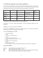
TABLE 1
Comparison of Sensitivity (Sens) for NMR Spectrometers
NMR Instrument, Probe
1
H
Sens (1)
19
F
Sens (2)
13
C
Sens (3)
31
U400, QUAD
(1H,19F,13C,31P)
5mm switchable
UI400, QUAD
(1H,19F,11B,31P)
U500, QUAD
(1H,19F,13C,31P)
VXR500, QUAD PFG Z
(1H,19F,13C,31P)
1
H{X} switchable
UI500NB
1
H{13C/15N} PFG Z
1
H{31P/X} PFG Z
15
N-31P BB (10mm)
UI600
1
H{13C/15N} PFG X,Y,Z
AutoX (15N-31P and 1H or
19
F)
15
N-31P BB (10mm)
~160:1
~150:1
~150:1
~110:1
Variable
Temperature
Range (oC)
-100 oC to +100 oC
~150:1
~90:1
-100 oC to +100 oC
-100 oC to +100 oC
~300:1
-100 oC to +100 oC
~200:1
-80 oC to +100 oC
VNS750NB
1
H{13C/15N} PFG X,Y,Z
15
N-31P BB (10mm)
13
C{1H} 5 mm
13
C{1H} 3 mm
~120:1
~120:1
~120:1
~260:1
~270:1
~150:1
~130:1
(disabled)
~210:1
~260:1
~280:1
~230:1
P
Sens(4)
~300:1
~210:1
-100 oC to +100 oC
~750:1
~700:1
NA
~80:1
NA
~550:1
-20 oC to +80 oC
-30 oC to +50 oC
-100 oC to +100 oC
~1000:1
~370:1
~475:1
~125:1
~320:1
-20 oC to +80 oC
-80 oC to +130 oC
NA
NA
~1100:1
~1350:1
~180:1
~1200:1
~530:1
~220:1
~206:1
-150 C to +150 C
~550:1
(~80:1
for 5mm tube)
~780:1
Numbers in ( ) indicate sample used, see corresponding list at the bottom.
(1) 1H Sensitivity Standard: 0.1% ethylbenzene/CDCl3 (5mm NMR tube)
(2) 19F Sensitivity Standard: 0.05% CF3C6H5/C6D6 (5mm NMR tube)
(3) 13C Sensitivity Standard: ASTM, 40% dioxane/C6D6 (5mm NMR tube)
(4) 31P Sensitivity Standard: 0.0485M Triphenylphosphate/CDCl3 (5mm NMR tube)
(5) For 10mm BB probe, 13C and 31P Sensitivity Standards are in 10mm NMR tube
3
-20 oC to +80 oC
-150 oC to +150 oC
-100 oC to +100 oC
-100 oC to +100 oC
B. Probe tuning for the hcn probe on UI500NB
Insert your sample into the magnet bore,
1) In the VNMR command line, type: tune(‘H1’,’C13’) or tune(‘H1’,’C13’,’N15’)
This sets the tuning CHAN 1 to 1H and CHAN 2 to 13C (and CHAN 3 to 15N)
2) Tune the 1H channel:
2-1. Disconnect the J5301 cable and connect it to J5321 on the Probe Tune Interface and
disconnect the J5302 cable and connect it to J5323 (Tune) on the Tune Interface.
2-2. Change CHAN to 1, by pushing the bottom button on the tune interface labeled +, leave the
setting on the right at 9. The TUNING INTERFACE readout should turn green and give a
reading.
2-3. Locate the large, shiny brass knob underneath the probe. It is labeled “Proton” and some red
`
4
color is visible on the knob. This proton adjustment knob has a large, lower, shiny portion and
a smaller, upper, knurled portion. The upper portion is for Tuning, while the lower portion is
for Matching. Turn these knobs, carefully in one direction and watch the output change on
the tune interface readout panel. If the readout increases, turn the Tune knob the other
direction, until a minimum value is reached. Adjust the Match knob to decrease the value
further. Continue to turn the tune and match knobs until you reach the smallest number
possible (ideally under 5, however, this is sample-and solvent-dependent).
2-4. Change CHAN back to 0
2-5. Return the cables back to their original positions (J5321 @J5301 and J5323 @J5302).
NOTE: DO NOT FORCE THE KNOB TO TURN. IF YOU FEEL RESISTANCE, STOP!
Otherwise, you could break the rod.
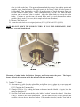
Placement of tuning knobs for Carbon, Nitrogen, and Proton under the probe. The largest,
brassy red knob is for proton and is the only one with tune and match.
3) Tune the 13C channel:
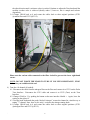
3-1. Disconnect the cable from the carbon filter on the floor (see the photo in the next page) and
connect it to J5321 on the Probe Tune Interface. Disconnect the J5312 cable and connect it to
J5323 (Tune) on the Tune Interface.
3-2. Change CHAN to 2, by pushing the button on the tune interface labeled +. Again, leave the
setting on the right at 9.
3-3. Turn the Green knob underneath the probe, labeled “carbon” to tune the channel. Note, there
is only 1 section to the carbon tuning knob. Turn this knob carefully in one direction and
watch the value on the tune interface readout. If this number increases, turn the Tune knob in
`
5
the other direction until a minimum value is reached. Continue to adjust the Tune knob until the
smallest readout value is achieved (ideally under 5, however, this is sample-and solventdependent).
3-4. Change CHAN back to 0 and return the cables back to their original positions (J5321
@carbon filter and J5323 @J5312).
Please note the carbon cable connected to the filter circled in green at the lower right-hand
corner.
NOTE: DO NOT FORCE THE KNOB TO TURN. IF YOU FEEL RESISTANCE, STOP!
Otherwise, you could break the rod.
4) Tune the 15N channel (if needed):
4-1. Disconnect the cable from the nitrogen filter on the floor and connect it to J5321 on the Probe
Tune Interface. Disconnect the J5312 cable and connect it to J5323 (Tune) on the Tune
Interface.
4-2. Change CHAN to 3, by pushing the button on the tune interface labeled +. Again, leave the
setting on the right at 9.
4-3. Turn the knob underneath the probe, labeled “nitrogen” to tune the channel in a similar way as
tuning 13C channel. Note, there is also only 1 section to the nitrogen tuning knob.
4-4. Change CHAN back to 0 and return the cables back to their original positions (J5321
@nitrogen filter and J5323 @J5312).
`
6
NOTES
Tuning and matching is performed to optimize sensitivity. Typically, 2D experiments take a long time
to acquire, and optimization of sensitivity can make the most effective use of the data acquisition time.
Greater sensitivity means larger signals.
The instrument is designed to measure 13C and 15N indirectly and these channels normally calibrated
by NMR lab staff. Consequently, the pw90 for the proton is the only pw that requires careful
calibration.
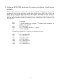
Typical Values on the Tune Interface Meter
Solvent
CDCl3
CD2Cl2
DMSO-D6
D2O
Proton
007
024
010
045
Carbon
001
002
002
001
Nitrogen
001
001
001
001
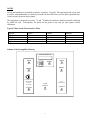
Scheme of the Preamplifier Housing
TUNE INTERFACE
XMTR
J5313
C
H
A
N
- 0
9
+ +
PROBE
A
T
T
N
J5321
XMTR
J5303
PROBE
PROBE
J5311
J5301
1/4 WAVELENGTH
BROADBAND
PREAMP
15-400 MZH
TUNE
OUTPUT
1H/19F
OBS PREAMP
OUTPUT
OUTPUT
J5323
J5302
J5312
`
7
C. Shimming
For 1D/2D gradient NMR experiments, you will be collecting your data without sample spinning.
Therefore you should shim your sample both in spinning and none spinning shims. The following is
the basic shim procedure, more can be found on the SCS NMR website. Again, this procedure is
written on the bases that you’ve trained on shimming previously when you first come to the NMR lab.
1) Load the system shim map by typing rts(‘hcn’) on the command line
2) Lock your sample by adjusting z0 value (check lockphase value also)
3) Shim spinning shims first (Z1 to Z5) while turning on the spin (spin rate at 20 Hz) by clicking spin
“ON” button
3-1. Adjust Z1 then, Z2, then Z1 again, iteratively. After the maximum lock signal (level) reaches,
3-2. Adjust Z3 (clockwise) to decrease the signal intensity about 20%, then adjust Z1 and Z2
(iteratively) to maximize the signal. Continue changing Z3 in the same direction if the lock
signal is higher than it was initially, and then adjust Z1 and Z2 until reach to maximum. It the
lock signal is worse, adjust Z3 (count-clockwise) to decrease the signal intensity about 20%,
then adjust Z1 and Z2 again.
3-3. Adjust Z4 as the same fashion as Z3 (step 3-2), that is, every change in Z4 must be followed
by the optimization of Z1 and Z2 until the highest possible lock level is obtained.
3-4. Adjust Z5. The best way is the same as above, or you can adjust the Z5 value to maximize the
lock signal, then check Z1 and Z2 again.
4) Repeat steps in step 3 iteratively until the highest possible lock level is obtained.
5) If you are satisfied with Z shims, turn off the spin by click spin “OFF” button, watch the lock
level. If the lock level drops more than 5 units, you need to shim the none-spinning shims (X1,
Y1, XZ, YZ, and XY and X2Y2).
4-1. Adjust X1 and Y1 iteratively to maximize the lock signal.
4-2. Adjust XZ in one direction to decrease the signal intensity about 20%. Adjust X1 to
maximize the signal. It it’s better, adjust XZ more in the same direction. If it becomes worse,
adjust XZ in the other direction until signal maximized.
4-3. Adjust YZ in one direction to decrease the signal intensity about 20%. Adjust Y1 to
maximize the signal as above.
4-4. Repeat step 4-1.
(Note: the following is non-routine)
4-5. Maximize lock level by shimming XY, then repeat step 4-1.
4-6. Maximize lock level by shimming X2Y2 then repeat step 4-5.
4-7. Repeat steps 4-1 to 4-3.
4-8. Repeat steps in step 3 (shim on Z again) with spin “ON”.
Finally if you have a good shimmed system, there should not be a big difference (< 10%) in lock
levels between sample spinning (spin=20 Hz) and none-spinning (spin=0). You may want to
collect a quick 1D proton spectrum to inspect the quality of the shims.
`
8
D. Setting up 1D/2D NMR experiments for structure elucidation of small organic
molecules
NOTE: These instructions assume that you will be collecting a full data set for structure
elucidation of small organic molecules, including both HMQC (inverse HETCOR) or HSQC and
HMBC (inverse long-range HETCOR) on the same sample. Instructions are also given for a
1D/2D TOCSY, NOESY or ROESY data collection. The experiment library will be as follows
(and you will have much less trouble if you always follow a routine such as this, in terms of your
data collection):
exp1:
exp2:
exp3:
exp4:
exp5:
1
H spectrum
H pw90 calibration or (optional) 13C spectrum with parameters for
gHMQC and/or gHMBC
2D 1H-1H gCOSY
2D 1H-13C gHMQC or 2D 1H-13C gHSQC
2D 1H-13C gHMBC
1
The following experiments are optional, but sometimes necessary
exp6:
exp7
exp8:
exp9:
exp10:
exp11:
exp12:
`
2D 1H-1H gDQCOSY
2D 1H-1H TOCSY
1D 1H-1H TOCSY
2D 1H-1H NOESY
1D 1H-1H NOESY1D
2D 1H-1H ROESY
1D 1H-1H ROESY1D
9
1. Setting up the 1H Experiment
1) Insert your sample in the spectrometer. Lock and shim the sample. NOTE: You can lock and
shim while the sample is equilibrating if the temperature change is <5°. However, you should
touch up the shims once the sample has equilibrated.
2) In exp1, set up parameters for a standard 1H experiment, set the temp parameter if you are going
to use VT, then enter su.
3) If using VT, wait until the temperature has reached the set point and your sample has equilibrated.
Then tune the probe according to the instructions. NOTE: You should have your parameters for a
standard 1H experiment loaded before tuning the probe, or alternatively type command tune(‘H1’)
or tune(‘1H’, ‘C13’) or tune(‘1H’,’C13’,’N15’) as described in probe tuning section on page 4.
5) Optimize the 1H parameters; mainly sw by setting the two cursors ~0.5 ppm beyond last proton
peak on both sides of spectrum, then type the command
movesw
2) Re-acquire 1D 1H experiment; make sure the parameters are correct. Then phase and reference the
1
H spectrum.
5) Determine the 1H pw90 of the sample (more details of this operation can be found at the SCS
NMR website named “90 Degree Pulse Width Determination”):
mf(1,2) jexp2 wft
gain?
A number will show up in the command line
gain=the number
Array experiment won’t run if you have gain=’n’
nt=1
type: array <rtn>
NOTE: The next four items are the answers to the questions posed by the array macro
Parameter to be arrayed: pw <rtn>
Enter number of steps in array: 10 <rtn>
Starting value: 20 <rtn> (an example. This number should be set to approximately
[(4*pw90 from the default setup) - 2)
Array increment: 1 <rtn>
Then type:
pw[1]=5
da
d1=10
ai vsadj vp=70
ga
`
Replaces first array element, 20, with the value 5 (for setting up the
correct phase)
Displays current arrayed values for pw
Sets absolute intensity mode and adjust the peak hight; places spectrum
about half-way up on the display.
Make sure gain = “a number”, do not use auto-gain
10
As the spectra accumulate, use dssh dssl to view them. You can terminate the experiment
with aa when you have determined the pw360 (where the signal is near zero).
NOTE: if the second spectrum is already positive, reset the array with a smaller starting value.
After you determine the pw360 of your sample,
jexp1
pw90=(the numeric value for the 360 found above!)/4; e.g., pw90=pw360/4
pw=pw90
ga
6) Quick determination of the T1 for the sample (more details of this operation can be found in the
SCS website named “T1 Measurement”):
NOTE: this step is optional. For most small molecules, 1.5 seconds of delay (d1) is normal. You
could use 2.0-2.5 seconds for optimal signal-to-noise)
mp(1,2) jexp2
gain=the number found previously
dot1 <rtn>
NOTE: The next three items are the answers to the questions posed by the dot1 macro)
Minimum T1 expected: 0.5 <rtn>
Maximum T1 expected: 5 <rtn>
Number of scans: 1 <rtn>
ga
As the spectra accumulate, use dssh to view them. You can terminate the experiment with aa
when you have determined the T1 of interest.
T1 = 1.443 x (null)
(Derived from M=Mo(1-2e-/T1)
M: magnetization at time after a 180 degree inversion pulse,
Mo: magnetization at equilibrium
(null): the time when the magnetization is zero)
7) To obtain the 1H spectrum used for the following experiments
jexp1
optimize d1 as necessary (based on the T1 if attempting a “good” integration (d1 ~ 5s))
optimize nt (nt ~ 8)
ga
Then phase, reference, and save the 1H spectrum.
`
11
2. Setting up the 2D 1H-1H gCOSY Experiment
The following setup assumes you have done steps 1-7 in Setting up the 1H Experiment. If you have
not, do them now before continuing.
1) To load a gCOSY experiment
jexp3
mf(1,3)
gcosy
2) check ni - it should be at least 256 for a typical spectral width of 10 ppm, but may be smaller for a
smaller sw.
Check:
d1=1-2 s or the value optimized in exp1 (~ 1.5T1)
pw=pw90
np=2048
sw1=sw
phase=1
nt=2 or multiple of 2 for better S/N
ni=128 or 256
if you change np or ni, readjust sb = -at/2 and sb1 = -ni/(2*sw1)
if you change np or ni, you may need to reset fn and fn1
3) Check time by typing time<rtn>, this experiment normally runs less than 10 mins for nt=2.
Adjust nt if necessary; there is no minimum.
Make sure the sample is not spinning!! To turn off, go to the VNMR Acquisition window, LC
Lock, LC spin off. While this window is open, make sure that the lock level is > 60% - you should
adjust only the gain, if possible. When you start the experiment with go (below), make sure that
the lock level stays above 20%.
enter
go to start
After the acquisition is complete, save your spectrum.
WORKUP: use wft2d to process.
Note:
The gradient gCOSY experiment provides homonuclear chemical shift correlation information via the
J-coupling interaction, revealing 2-bond (germinal) and 3-bond (vicinal) spin-spin coupled pairs.
Sensitivity of this experiment is not normally an issue; it is acquired and processed in absolute value
(magnitude) mode and usually requires no more than a few minutes to acquire. Other COSY type
experiments are given later in the document; the gradient double-quantum filtered phase-sensitive
COSY experiment, gDQCOSY, provides information about the adjacent two spin systems. TOCSY
experiment has a very good S/N ratio, revealing the spin-spin correlation throughout the spin systems
in a molecule. TOCSY1D: 1D version of 2D TOCYS; giving a clean one spin-spin system at a time.
`
12
3. Setting up the 2D 1H-13C gHMQC (or gHSQC) Experiment
The following setup assumes you have done steps 1-7 in Setting up the 1H Experiment. If you have
not, do them now before continuing. You should have an optimized 1H spectrum setup in exp1 before
proceeding with the setup below.
1) (Optional) jexp2 and set up parameters for a standard 13C experiment (nt=1 or 4 should be
sufficient to see the solvent peak). Acquire a spectrum with ga, then phase and reference. Check
sw and change with movesw if desired. Remember, if you are only acquiring an HMQC
spectrum, you can narrow the 13C sw to include only protonated carbons. If you are also acquiring
an HMBC spectrum, the sw should be set for both protonated and quaternary carbons. Please also
remember that the pw90 of 13C needs to be calibrated but this has already done on a standard
organic sample by NMR staff, you can use the default 13C values. Please talk to the NMR staff if
you want to calibrate the 13C data on your particular sample.
2) To load a HMQC (or HSQC) experiment
jexp4
mf(1,4)
ghmqc (or gHSQC)
(enter the answers accordingly)
3) Check parameters
at should be around 0.2 seconds (np ~ 2048)
d1 should be set so that:
a) at/(at+d1) < 0.15
THIS CONDITION MUST BE MET! If necessary,
reduce np (i.e., np=np/2) and/or increase d1.
b) d1+at = 1 to 1.5 x T1 This is a recommendation. If your T1's are long, you can
try the default setting of d1=2. If you set d1 for less than
the recommended time, you will sacrifice sensitivity.
However, if your sample concentration is adequate, the
savings in time will more than balance this loss.
nt should be set according to sample concentration, no minimum required (2 or 4 is adequate).
ni should be set between 256 and 512.
phase=1,2
4) By default, j1xh=140, which is the average one-bond 1H-13C coupling constant for your sample.
If you do not see a correlation you believe should be visible, it may be because the coupling
constant for this particular C-H bond differs too much from this average value. If you re-run the
experiment optimized for the new coupling constant, the correlation should appear.
5) If you chose to set 13C parameters manually, set the following:
sw1 = (sw of 13C spectrum collected previously in step 1, otherwise use the default value)
dof = (tof of 13C spectrum collected previously in step 1, otherwise use the default value)
6) check time, adjust nt if necessary
(It normally take 20-40 min depending sample concentration)
`
13
Make sure the sample is not spinning!! To turn off, go to the VNMR Acquisition window, LC
Lock, LC spin off. While this window is open, make sure that the lock level is > 60% - you should
adjust only the gain, if possible. When you start the experiment with go (below), make sure that
the lock level stays above 20%.
enter dps to check the pulse sequence
enter go to start
After the acquisition is complete, save your spectrum.
WORKUP: use wft2da to process; use twod to setup proper display window.
The difference between HMQC and HSQC
Both 1H-13C HMQC (Heteronuclear Multiple Quantum Coherence, eg. 2IxSy) and HSQC
(Heteronuclear Single-Quantum Coherence, eg. 2IzSx) detect the correlation between directly bonded
1
H and 13C nuclei via the one-bond 1H and 13C J coupling interaction. The cross peaks in the 2D
spectrum contain both chemical shifts information of the carbon and its directly attached protons,
providing a correlation map between the coupled spins.
HMQC has shorter relaxation pathway and is more robust to poorly calibrated pulses. However the
cross peaks are modulated by homonuclear proton J coupling which broadens the carbon dimension.
All cross peaks in HMQC spectrum have the same sign.
HSQC cross peaks are not affected by homonuclear proton J coupling and has a superior resolution in
the carbon dimension. The edited gradient-enhanced HSQC (gHSQC) inverts the CH2 signals, leaving
these cross peaks negative. The CH and CH3 cross peaks are positive in the 2D spectrum. If you work
with a well calibrated system, gHSQC is preferred.
`
14
4. Setting up the 2D 1H-13C gHMBC Experiment
The following setup assumes you have done steps 1-7 in Setting up the 1H Experiment.
1) To load a gHMBC experiment
jexp5
mf(1,5)
ghmbc
(enter the answers accordingly)
2) Check parameters
nt should be 4 to 8 times of that necessary for the gHMQC experiment,
ni should be set between 256 and 512.
pw=pw90
phase=0
jnxh=8 is the default value, the average long range 1H-13C coupling constant. Typical values
are between 5 and 10. If you are missing some correlations, you may need to run the
experiment again with a different value of jnxh.
By default, j1xh=140, the average one-bond 1H-13C coupling constant for aliphatic
proton/carbon pairs, aromatic 1-bond 1H-13C coupling constants are 170-250 Hz, so j1xh=180
if you want to filter out one-bond 1H-13C aromatic peaks.
3) check time, adjust nt if necessary (It normally takes 1-12 hrs depending on sample concentration)
Make sure the sample is not spinning!!
enter dps to check the pulse sequence
enter go to start
After the acquisition is complete, save your spectrum.
WORKUP: use wft2da to process; use twod to setup proper display window.
`
15
5. Setting up the 2D 1H-1H gDQCOSY Experiment
The following setup assumes you have done steps 1-7 in Setting up the 1H Experiment. If you have
not, do them now before continuing.
1) To load a gDQCOSY experiment
jexp6
mp(1,6)
gDQCOSY
2) check ni - it should be at least 256 for a typical spectral width of 10 ppm, but may be smaller for a
smaller sw.
Check:
d1=1-2 s or the value optimized in exp1
pw=pw90
np=4096
nt=4 or multiples of 4 for greater S/N
sw1=sw
phase=1,2
ni=200 or 256 or more
if you change np or ni, readjust sb = -at/2 and sb1 = -ni/sw1, and sbs = -at/2 and sbs1=-ni/sw1
(squared sine bell with 90 degree shift)
if you change np or ni, you may need to reset fn and fn1
3) Check time, this experiment normally runs less than 20 mins for nt=4. Adjust nt if necessary.
Make sure the sample is not spinning!! To turn off, go to the VNMR Acquisition window,
LC Lock, LC spin off. While this window is open, make sure that the lock level is > 60% you should adjust only the gain, if possible. When you start the experiment with go (below),
make sure that the lock level stays above 20%.
enter
go to start
After the acquisition is complete, save your spectrum.
WORKUP: use wft2da to process.
Note:
The gradient double-quantum filtered phase-sensitive COSY (gDQCOSY) removes the intense
singlets and observes only the magnetization associated with double-quantum coherence multiplets.
The diagonal peaks are in absorption mode, giving much narrow diagonal peaks compared with
gCOSY which has dispersive diagonal peaks. Therefore gDQCOSY presents less interference to the
cross peaks near the diagonal. This experiment reveals germinal and vicinal spin-spin coupled pairs
and measures the proton-proton J coupling constants. However its S/N is half of that of gCOSY
therefore twice as many scans are needed to achieve the same S/N as in gCOSY.
`
16
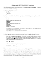
Example: Measurement of proton-proton J coupling constants*
*: from “Modern NMR Spectroscopy, a guide for chemists” by J. Sanders and B. Hunter, 2nd Edition
(Oxford University Press), Page 116.
`
17
6. Setting up the 2D 1H-1H TOCSY Experiment
The TOCSY mixing time, m, is related to how far the spin-spin relay carries throughout the spin
system, in the range of 60-100ms, is typically useful to observe 4- and 5-bond coupling correlations.
Its default value is 80 ms for a small molecule of size less than 1000 da. The larger the molecule is,
the shorter of the mixing time.
The following setup assumes you have done steps 1-7 in Setting up the 1H Experiment. If you have
not, do them now before continuing.
1) To load a TOCSY experiment
jexp7
mp(1,7)
TOCSY
2) Check ni - it should be at least 256 for a typical spectral width of 10 ppm, but may be smaller for a
smaller sw.
Check:
d1=1-2 s or the value optimized in exp1
pw=pw90
np=4096 (or smaller, e.g. 2048)
nt=2 or multiples of 2 for greater S/N
sw1=sw
phase=1,2
ni=200 or 256 or more
mix=0.08 (80 ms) or other value as described above
if you change np or ni, readjust sb = at/2 and sb1 = ni/(2*sw1)
if you change np or ni, you may need to reset fn and fn1
3) Check time, this experiment normally runs less than 20 mins for nt=2. Adjust nt if necessary.
Make sure the sample is not spinning!! To turn off, go to the VNMR Acquisition window,
LC Lock, LC spin off. While this window is open, make sure that the lock level is > 60% you should adjust only the gain, if possible. When you start the experiment with go (below),
make sure that the lock level stays above 20%.
enter
go to start
After the acquisition is complete, save your spectrum.
WORKUP: use wft2da to process.
`
18
7. Setting up the 1D 1H-1H TOCSY Experiment
1D TOCSY1D is a one-dimensional version of 2D TOCSY. By selectively irradiating one proton with
soft shaped pulse, only its spin-spin correlation to other protons can be detected. This 1D experiment has
advantages over 2D experiment by eliminating potential overlaps to provide an effective and clean
TOCSY spectrum.
The following setup assumes you have done steps 1-7 in Setting up the 1H Experiment. If you have not,
do them now before continuing.
1) To load a 1D TOCSY experiment
jexp8
mf(1,8)
wft full
pw=pw90
TOCSY1D(‘ds’)
2) Expand around first peak to be irradiated (inverted). Center cursors around desired peak ensuring that
the full peak is between the two cursors, then,
LC Select
Selects current region between cursors for selective inversion
Repeat Select for all desired peaks. When completed,
LC Proceed
Calculates shaped pluses and completes TOCSY1D setup
You will need to answer the following questions:
Enter reference 90 degrees pulse with (sec):
Enter your determined pw90 from pw90 calibration you’ve done early
Enter reference power level:
Enter the tpwr value used in pw90 calibration
da
Displays array. Make sure all your desired peaks have been selected.
They will appear with name similar to TOCSY1D_5_67p.RF, where
the numbers refer to the chemical shift of the peak.
3) Check
nt=16 (or 32 for a better S/N)
d1; normally ~ 2 seconds (or longer)
mix=0.08 (80ms) or other value as describe in 2D TOCSY section
4) Check time, adjust nt if necessary.
Make sure the sample is not spinning!!
enter
`
go to start
19
After the acquisition is complete, save your spectrum.
WORKUP: use wft to process.
Do not auto-phase the spectrum (aph). First type phase(180) (if necessary) to have the irradiated peak
in the positive direction, then phase manually, the TOCSY peaks will be in the same positive direction.
dssh or dssa to view all spectrum in array
To view individual spectrum, type ds(#), where # is the number of the desired spectrum.
To print all spectra in the array:
pl(‘all’) pscale page
To print individual spectrum:
ds(#)
pl pscale page
or
pl pir ppf pscale page (add ppf or pir for peak picking and integration)
`
20
8. Setting up the 2D 1H-1H NOESY Experiment
1
1
The 2D H- H NOESY experiment measures NOE (Nuclear Overhauser Enhancement) between protons
within a molecule, providing information about distance between two protons in space. The stronger the
NOE is, the closer of the two nuclei locate.
Sign of NOE cross peaks:
(1) For small organic molecule, all NOE cross peaks have the opposite phase to the diagonal
peaks, in contrast the cross peaks from chemical or conformational exchange are in phase with
the diagonal.
(2) For large molecules, all NOE cross peaks and the exchange cross peaks are in phase with the
diagonal. In such case, ROESY experiment can be perform to distinguish between them if
needed.
The following setup assumes you have done steps 1-7 in Setting up the 1H Experiment. If you have not,
do them now before continuing.
1) To load a NOESY experiment
jexp9
mf (1,9) wft full
pw=pw90
NOESY
2) Check parameters
nt=32 (or more for better signal-to-noise ratio)
ni=200 or more for a typical spectral width of 10 ppm, but may be smaller for a smaller sw
(e.g. ni=200).
sw1=sw
d1=~ 2 seconds (or longer)
phase=1,2
mix=0.25 – 0.5 (250 – 500 ms), the mixing time for the NOE build-up. The mixing time is
correlated to the molecular weight of the molecule. Generally 300 ms is adequate
for MW > 1000, and ~500 ms for MW < 1000. If a mixing time is too short, it will
not allow the NOE to buildup; if a mixing time is too long, it results in spin
diffusion and you will get feak NOE peaks. Sometimes, a couple of NOESY
experiments are collected for different mixing time. mix=0.5 (500ms) is the default
value.
3) Check time, adjust nt if necessary;
Make sure the sample is not spinning!!
enter
go to start
After the acquisition is complete, save your spectrum.
WORKUP: use wft2da to process.
`
21
9. Setting up the 1D 1H-1H NOESY Experiment
1
1
1D H- H NOESY is a one-dimensional version of 2D NOESY. By selectively irradiating one proton
with soft shaped pulse, only its NOE to other protons can be detected. This 1D experiment has
advantages over 2D NOESY experiment by eliminating potential overlaps to provide an effective and
clean NOE spectrum.
The following setup assumes you have done steps 1-7 in Setting up the 1H Experiment. If you have not,
do them now before continuing.
1) To load a 1D NOESY experiment
jexp10
mf(1,10) wft full
pw=pw90
NOESY1D(‘ds’)
2) Expand around first peak to be irradiated (inverted). Center cursors around desired peak ensuring that
the full peak is between the two cursors, then,
LC Select
Selects current region between cursors for selective inversion
Repeat Select for all desired peaks. When completed,
LC Proceed
Calculates shaped pluses and completes NOESY1D setup
You will need to answer the following questions:
Enter reference 90 degrees pulse with (sec):
Enter your determined pw90 from pw90 calibration you’ve done early
Enter reference power level:
Enter the tpwr value used in pw90 calibration
da
Displays array. Make sure all your desired peaks have been selected.
They will appear with name similar to NOESY1D_5_67p.RF, where
the numbers refer to the chemical shift of the peak.
3) Check
nt=64 (or 128, or 256.. for a better S/N)
d1; normally ~ 2 seconds (or longer)
mix=0.5 (500ms) or other value as describe in 2D NOESY section
4) Check time, adjust nt if necessary;
5) Set bs=16 (or 32), il=’y’ so that the data will be collected for the first FID (first arrayed peak) in
the block size of 16 (or 32), then go to the second FID….. instead of finishing the first FID (first
arrayed peak) then go to the second arrayed peak. Such if the S/N is good enough, you can always
stop the experiment.
Make sure the sample is not spinning!!
`
22
enter
go to start
After the acquisition is complete, save your spectrum.
WORKUP: use wft to process.
Do not auto-phase the spectrum (aph). First type phase(180) (if necessary) to have the irradiated peak
in the negative direction, then phase manually, the NOESY peaks will be in the positive direction, and
exchange peaks will in the negative direction for small molecules.
dssh or dssa to view all spectrum in array
To view individual spectrum, type ds(#), where # is the number of the desired spectrum.
To print all spectra in the array:
pl(‘all’) pscale page
To print individual spectrum:
ds(#)
pl pscale page
or
pl pir ppf pscale page (add ppf or pir for peak picking and integration)
`
23
10. Setting up the 2D 1H-1H ROESY Experiment
The ROESY (Rotating frame Overhauser Effect Spectroscopy) experiment measures NOE in the rotating
frame, providing information about distance between two protons in space. It is generally used for
compounds with a molecular weight of 1000-3000 for which NOESY is approximately close to zero.
ROESY cross peaks are always having opposite sign to the diagonal peaks, contrary to any TOCSY or
exchange peaks if exists in the ROESY spectrum.
The following setup assumes you have done steps 1-7 in Setting up the 1H Experiment. If you have not,
do them now before continuing.
1) To load a ROESY experiment
jexp11
mf(1,11) wft full
pw=pw90
ROESY
2) Check parameters
nt=32 (or more for better signal-to-noise ratio)
ni=200 or more for a typical spectral width of 10 ppm, but may be smaller for a smaller sw
(e.g. ni=200).
sw1=sw
d1=~ 2 seconds (or longer)
phase=1,2
mix=0.1 – 0.3 (100 – 300 ms), the mixing time for the ROE build-up. The mixing time is
correlated to the molecular weight of the molecule. Long mixing time is needed for
a small molecule. Generally 100-150ms is adequate for MW ~400-2000, and 200300 ms if you want to observe longer mixing time ROE; for MW < ~ 400, 300-500
ms for long mixing time is generally used. All ROE cross peaks are in the opposite
sign of the diagonal peaks, while TOCSY or exchange peaks are in phase with the
diagonal. mix=0.2 (200ms) is the default value.
3) Check time, adjust nt if necessary
Make sure the sample is not spinning!!
enter
go to start
After the acquisition is complete, save your spectrum.
WORKUP: use wft2da to process.
`
24
11. Setting up the 1D 1H-1H ROESY Experiment
1D ROESY1D is a one-dimensional version of 2D ROESY (Rotating frame Overhauser Effect
Spectroscopy) experiment. By selectively irradiating one proton with soft shaped pulse, only its ROE to
other protons can be detected. This 1D experiment has advantages over 2D ROESY experiment by
eliminating potential overlaps to provide an effective and clean ROE spectrum.
The following setup assumes you have done steps 1-7 in Setting up the 1H Experiment. If you have not,
do them now before continuing.
1) To load a 1D ROESY experiment
jexp12
mf(1,12) wft full
pw=pw90
ROESY1D(‘ds’)
2) Expand around first peak to be irradiated (inverted). Center cursors around desired peak ensuring that
the full peak is between the two cursors, then,
LC Select
Selects current region between cursors for selective inversion
Repeat Select for all desired peaks. When completed,
LC Proceed
Calculates shaped pluses and completes ROESY1D setup
You will need to answer the following questions:
Enter reference 90 degrees pulse with (sec):
Enter your determined pw90 from pw90 calibration you’ve done early
Enter reference power level:
Enter the tpwr value used in pw90 calibration
da
Displays array. Make sure all your desired peaks have been selected.
They will appear with name similar to ROESY1D_5_67p.RF, where
the numbers refer to the chemical shift of the peak.
3) Check
nt=64 (or 128, or 256.. for a better S/N)
d1; normally ~ 2 seconds (or longer)
mix=0.2 (200ms) or other value as describe in 2D ROESY section
4) Check time, adjust nt if necessary.
5) Set bs=16 (or 32), il=’y’ so that the data will be collected for the first FID (first arrayed peak) in
the block size of 16 (or 32), then go to the second FID….. instead of finishing the first FID (first
`
25
arrayed peak) then go to the second arrayed peak. Such if the S/N is good enough, you can always
stop the experiment.
Make sure the sample is not spinning!!
enter
go to start
After the acquisition is complete, save your spectrum.
WORKUP: use wft to process.
Do not auto-phase the spectrum (aph). First type phase(180) (if necessary) to have the irradiated peak
in the negative direction, then phase manually, the ROESY peaks will be in the positive direction, and
exchange peaks will in the negative direction for small molecules.
dssh or dssa to view all spectrum in array
To view individual spectrum, type ds(#), where # is the number of the desired spectrum.
To print all spectra in the array:
pl(‘all’) pscale page
To print individual spectrum:
ds(#)
pl pscale page
or
pl pir ppf pscale page (add ppf or pir for peak picking and integration)
`
26
E. Guideline for 2D Data Acquisition
You can make a good approximation of the number of scans needed for your 2D data acquisition by
looking at your 1D 1H spectrum. The 1H 1D spectrum needs to be acquired under the following
conditions:
1.
2.
3.
4.
pw=pw90
nt=1
Check the S/N to the smallest peak of interest in your spectrum.
Check that number versus the suggested numbers below.
gcosy:
if the S/N > 50:1, use nt=1; the experiment time is ~ 5 minutes
ghmqc:
if the S/N > 250:1, use nt=1; the experiment time is ~ 15 minutes
if the S/N > 100:1, use nt=4; the experiment time is ~ 1hour
ghmbc:
if the S/N > 250:1, use nt=8; the experiment time is ~ 45 minutes. It should be 4 to 8
times of that necessary for the gHMQC experiment.
Note:
In a 1D experiment, if you want to double the S/N, you need to increase 4 times nt used.
`
27
F. 2D Data Processing (This section will be expanded later)
Unless you have been informed of a macro that will do the proper data processing of your spectrum
for you, you will need to process the data manually. Below is a table showing the optimum processing
apodizations (window functions), and the proper processing commands in Vnmr software.
Experiments
Apodization 1
Apodization 2
Processing
gCOSY **
(phase=1)
TOCSY
(phase=1,2)
gHMQC
(phase=1,2)
gHMBC
(phase=0)
sb=-at/2
sb1=-ni/(2*sw1)
gf=at/2
gf1=ni/(2*sw1)
wft2d('t2dc','1,0,0,1')
foldt (optional)
wft2da
gf=at/2
gf1=ni/(2*sw1)
wft2da
gf=at/2
gf1=ni/(2*sw1)
av av1 wft2da
Process
Shortcut
wft2d
foldt
**For gCOSY, gf=at/2 and gf1=ni/(2*sw1) can be used to enhance S/N
For plotting, you can use cosyplot and hetcorplot.
information.
Check the appropriate handouts for more
cosyplot can be used on the instrument or the SUNDS.
If you want to use hetcorplot, you need to have acquired a “good” 1D 13C spectrum on an instrument
other than the ui500nb. You can then plot on the SUNDS.
To plot using hetcorplot on the SUNDS:
1. logon to the ui500nb
2. jexp1
3. load your 1D 1H fid and process
4. jexp4
5. load your ghmqc data and process
6. logon to the instrument with your 1D 13C fid
7. jexp2
8. load your 1D 13C fid and process
9. jexp4
10. dconi to display 2D data
11. set the window as you want, then type hetcorplot and answer the questions as appropriate.
Some useful commands:
pcon page
dconi
fullt
vs2d
`
used to plot 2D spectrum as displayed on the screen
used to redisplay 2D after changes, e.g., vs2d
sizes the 2D display so that 1D spectra can be plotted on the side and top of the 2D plot
used to rescale the 2D plot; used dconi after using this command
28
Supplemental material on processing 2D spectrum:
1) At end of experiment, set appropriate weighting functions and linear prediction parameters, type
commands:
setLP1
sqsinebell
2) If fn parameter now equals 4096, process will be slow, then type:
fn = np
fn1 = fn
3) Switch f1 and f2 axes (make f2 the x-axis), type
trace = 'f2' or trace = ‘f1’
4) Display full across screen (removes error message)
full
5) Display full ppm scale
f
6) Display as contour plot, type command:
dp10
7) Spectrum should be appropriately referenced already, but you should confirm this; if necessary rereference by putting cursor on appropriate diagonal peak and type (assuming CDCl3):
rl(7.26p)
rl1(77d)
dp10
8) Adjust vertical scale with vs +20% and vs -20% menu buttons or with middle mouse button or
manually changing the parameter, vs2d, so vs2d = 100 (the lower the number, the less noise displayed),
then redraw 2D with dp10 command
9) Print with full rectangle, type:
full
dp10
pcon(10,1.2) page
10) Save data, type:
svf('filename')
`
29
G. Chemical Shift Referencing:
1
H Spectrum:
You can use either an internal chemical shifts standard (e.g. TMS: 0 ppm) or a residual 1H resonance
from the deuterated solvent (e.g. 7.26 ppm for CDCl3). Less commonly you can use a capillary
containing a standard to avoid any chemical shifts changes due to solvent conditions such as pH and
concentration etc.
11
B Spectrum:
The commonly used 11B chemical shift standard is 15% (v/v) BF3.OEt2 in CDCl3, and is referenced to
0.0 ppm. When you use the standard parameter loaded from the manual bar, the BF3.OEt2 in CDCl3
will appeared at 0.0 ppm.
13
C Spectrum:
Commonly a residual 13C resonance from the deuterated solvent is used as the reference.
19
F Spectrum:
The chemical shift standard for 19F is neat CFCl3, which is referenced to 0.0 ppm; which giving TFA
at -73.6 ppm, or 0.05% C6H5CF3 in C6D6 at -62.9 ppm.
31
P Spectrum:
85% phosphoric acid (H3PO4) in D2O is used, giving a reference peak at 0.0 ppm, or 0.0485M
triphenyl phosphate in CDCl3 is reference at -17.9 ppm with respect to the phosphoric acid.
15
N Spectrum:
Different referencing schemes have been in common use as reported in literature. Setting the chemical
shift of nitromethane at 0.0 ppm results in most compounds have negative values of 15N resonances.
The chemical shift of liquid ammonia (used for bio-samples) is 380 ppm away from nitromethane
(used for organic compounds). Here is the table listing the 15N Chemical shifts expressed with respect
to both reference compounds.
Chemical Shift Referencing Schemes for 15N
Compound
(NH3)
Amines
-49
NH3
0
NH4NO3
21
NH4Cl
39
Amides
119
CH3CN
243
Nitriles
258
Pyridine
319
Imines
343
NH4NO3
376
CH3NO2
380
Nitrates
388
`
(CH3NO2)
-429
-380
-359
-341
-261
-137
-122
-61
-37
-4
0
8
30
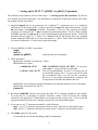
H. Structure Elucidation: Quinine as an Example
Quinine
N
OH
O
N
Chemical Formula: C20H24N2O2
Exact Mass: 324.18
Molecular Weight: 324.42
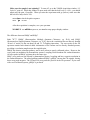
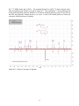
H-1: 1H NMR proton data (CDCl3): The results of 1H NMR spectroscopic analysis (Figure H-1) are
consistent with the structure of Quinine. A total of 23 protons were observed examined by integration
with a long T1 recovery delay (The OH proton was missing in the spectrum due to its broadness)
including 5 aromatic protons, 3 vinyl protons, and 15 aliphatic protons. The aliphatic protons was
further separated to 4 methine, 4 methylene groups and 1 methyl group as drawn from logic of further
work shown below.
Figure H-1: Proton Spectrum of Quinine.
`
31
H-2: 13C NMR carbon data (CDCl3): The Attached Proton Test (APT) 13C data collected with a
fully decoupled proton domain is present in Figure H-2. The J-modulated 13C data exhibit up and
down peaks depending upon the numbers of its directly attached protons giving CH and CH3 up
and CH2 and quaternary carbons down or vice versa. A total of 20 carbon peaks were observed,
consistent with the structure of Quinine.
Figure H-2: Carbon-13 spectrum of Quinine
`
32
H-3: 1H-1H NMR 2D gCOSY data (CDCl3): The data developed from the 2D gCOSY experiment are
illustrated in Figure H-3. These data reveal isolated contiguously coupled spin systems. Two
aromatic spin systems and one continuously coupled spin system (including aliphatic and vinyl
protons) are observed.
Figure H-3: 1H-1H 2D gCOSY spectrum of Quinine
`
33
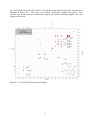
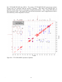
H-4: 1H-13C NMR 2D HSQC data (CDCl3): The data developed from the 2D 1H-13C HSQC
experiment are illustrated in Figure H-4. These data reveal one bond cross correlations between
protons and carbons in a two dimensional format. Assignments in either domain allow direct
assignment of the opposite domain from their cross contours. The assignments illustrated in Figure
H-4 are based upon data and conclusions obtained from other experiments, i.e. 2D gCOSY and 1D
APT carbon data, chemical shifts and coupling constant considerations. These data are consistent
with the structure of Quinine.
Figure H-4: 1H-13C 2D HSQC Spectrum of Quinine
`
34
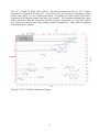
H-5: 1H-13C 2D HMBC data (CDCl3): The data developed from the 2D HMBC experiment are
illustrated in Figure H-5. These data reveal multiple-bond cross correlations between protons and
carbons in a two dimensional format. The assignments illustrated in Figures H-5 are primarily from 3bond proton-to-carbon cross correlations. The experiment is optimized with a time delay for 8 Hz
coupling (3JHC coupling). Occasionally 2-bond and 4-bond correlations will appear. Furthermore, the
suppression on one-bond couplings also appears in the spectra due to non-optimal bird-pulse
suppression. Some of the important 3-bond correlations are summarized in the structural illustration
below:
Figure H-5: 1H-13C 2D HMBC Spectrum of Quinine
`
35
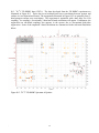
H-6: 1H-1H NMR 2D NOE data (CDCl3): The results of 1H-1H NMR 2D NOE spectroscopic analysis
(Figures H-6) are consistent with the structure of Quinine. These data reveal through space or
proximal located spins and are based upon relaxation phenomenon. Thus, strong NOE observed
between protons 2 and 5, and strong NOE observed between protons 9 and 3 suggest that the relative
stereochemistry of this compound is as shown.
Figure H-6: 1H-1H 2D NOESY Spectrum of Quinine
`
36