Download Inova600 Cold Probe User Manual

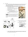
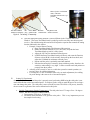
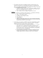
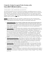
Using the Varian Cryogenic Probe System on the
Inova-600 NMR Spectrometer
(Generally called the “Cold-Probe” or “Chili-Probe” in the Varian vernacular)
-Thursday, March 11, 2004, by Rich Shoemaker (corrected 9/27/07)
This manual is intended for users who are experienced at operating the Varian NMR spectrometers at a relatively
high level of proficiency. The intent is to point out the issues pertaining to the cold-probes, how the use of the coldprobe differs from a conventional probe, and the issues that directly affect how one does spectroscopy with these
probes. Issues pertaining to the proper care and use of the cold-probe system, to ensure that the equipment is not
damaged will also be discussed. (Note: Many of the pictures & figures have been taken from the Varian Cold-Probe
Manuals, and have been used with permission.)
Overview: Doing NMR spectroscopy with a cold-probe is essentially the same as with a conventional probe;
however, certain properties of the cold-probe must be understood to obtain optimal results. Each of these will be
address in further detail later in this document. The primary issues that should be understood are:
•
•
•
•
•
Rf Pulse Ringdown Times: Due to the high “Q” (Quality-factor) of these probes, the ring-down time of the
tuned circuit is significantly longer. This means that the delay between the end of the pulse, and start of
signal detection is longer. Since pre-acquisition delays can adversely effect the appearance of the spectrum
(mostly in frequency-dependent phase errors, and other baseline issues), there are new parameters that deal
with this problem. The parameter “qcomp” (for Q-compensation) is used, and is dependent upon the
settings of the “dsp” parameter.
Rf Power Handling: The cold-head in the probe is maintained at a precise temperature through a process of
super-cooling helium gas in the cold-loop, and then an Intelligent Temperature Controller (ITC) re-heats the
probe-head to maintain a stable temperature (25.0 Kelvin under normal operation). When Rf power is
inserted into the probe (especially under broadband decoupling, i.e. 15N and 13C), this causes heating. The
ITC detects these fluctuations, and compensates by dropping the current through the heater. The heater
power (in Watts) is displayed in the CryoBay Monitor window. As the net Rf power in an experiment
increases, the heater power will drop to maintain a steady probe-head temperature of 25.0 Kelvin. If too
much power is used, such that lowering the heater power cannot maintain the probe-head temperature, then
the tuning will be lost, and ultimately damage to the probe (or the receiver pre-amplifier in the probe) could
occur!
Pulsed Field Gradient Performance: The inductance of the gradient coil in these probes is much higher.
Adjustments have been made to the gradient amplifier to compensate for this; in addition, the software has
built-in, rudimentary shaping of the rise/fall times of the gradient pulses to further improve the gradient
performance (esp. the amplitude stability). A new parameter called “gradientshaping” (a global “flag”
parameter) is used to activate the shaping of the gradient pulses.
Instrument Cabling: Since the first-stage proton observe pre-amplifier is inside the cryogenically cooled
region of the probe, a different receiver pre-amplifier module (called a “Cryopreamp Driver”) is installed.
The way this system is setup for operation and probe tuning is different. Furthermore, no Rf filters can be
inserted between the HBPROBE/XMTR output (J5331) and the proton input of the probe. Cabling for
tuning the 1H channel is also different.
Probe Tuning: In addition to cabling issues, the cold probe has a different user-interface for probe tuning. A
single brass knob is used to tune all channels. A larger knob is used to position the tuning stick to engage the
tuning element for each channel. Tuning channels are available for 1H Tune, 1H Match, 13C Tune, 15N Tune,
and 2H Tune.
Description of the Cryogenic Probe System:
Everyone using the cold-probe system should have a basic understanding of how the system functions, and what the
basic components are. Figure 1 below illustrates the entire cold-probe system, with the key parts labeled. The basic
theory of operation is as follows:
•
•
•
•
Helium gas is compressed by the compressor in the CryoBay. The compressed helium undergoes thermal
expansion in the Closed Cycle Chiller (CCC), which is the box in the corner of the 600 magnet room (near
the hole in the wall).
Inside the CCC, the cold-head is cooled to well below 25 Kelvin. Part of the compressed helium is split-off
and routed through the cold-head in the CCC, is cooled to below 25 Kelvin, and flows through the flexible
line to the side-arm of the probe, and up through the probe.
Figure 2 illustrates the path of the cold helium in the “cold-loop”, as the internal components of the probe
(the tuning elements, the coils, and the receiver pre-amplifier) are cooled.
All of this is maintained at ~10-8 Torr vacuum to achieve thermal isolation from the outside world (meaning
the sample and the magnet components outside the probe are kept at or near room temperature).
Figure 1: Cold-Probe System Diagram
•
•
The Intelligent Temperature Controller (ITC)
uses a variable heater in the probe assembly to
maintain the desired temperature at the
coldhead.
Note: even though the sample is relatively
well insulated from the cryogenic
temperatures inside the cold-probe, it is
imperative that dry air be flowing through the
VT-port in the probe. Without VT air-flow,
the sample will cool at a rate of ~10C. per
minute (until it freezes).
Figure 2: Diagram of the Cold-Probe
2
Performing NMR Experiments with the Cold Probe:
Once the cold-probe system has been properly installed, and is fully stabilized at the operating temperature of 25
Kelvin, doing NMR is not much different than a normal probe. The CryoBay Monitor window will indicate
“READY” when the system is ready to use. The issues outlined in the “Overview” section above will be discussed
in detail below.
I.
Monitoring the Status of the Cold-Probe system: CryoBay Monitor Status Window:
a. When operating, the CryoBay always displays the status of the system. Figure 3 illustrates the
CryoBay Monitor Status window, showing all of the key elements of the window.
Figure 3: CryoBay Monitor
Current Temperature at the ColdHead
(this is the coil temperature, and should
not change more than +/- .5 degrees)
If “cooling” will show time remaining until ready.
Cold-Loop-Impedance (related to Helium mass flow)
Heater Power (Watts) being applied to maintain Temp.
Cryo-System Status: Must be “READY” to use.
II.
Instrument/Probe Cabling:
a. Cabling for 13C, 15N, and 2H is the same as a conventional probe, including the location of the
bandpass filters.
b. 1H cabling is different. Refer to Figure 3, and the following instructions to ensure that the system is
cabled properly.
i. The cable from the High-Band Transmitter plugs into
From
the top port “HB XMTR (J5303)”
ii. HBPROBE XMTR (J5331) goes to the “1H XMTR”
HB amplifier
port on the probe.
To
iii. HB PROBE/PREAMP (J5335) connects to the “1H
RCVR” port on the probe.
probe 1H
iv. OUTPUT (J5302) is connected to the same cable as a
normal pre-amplifier (Output cable connects to the
mixer in the magnet leg interface).
v. Signal path:
1. The transmitter pulse is routed to the probe
from port J5331 on the cryopreamp driver to
From Probe
the probe. This cable (a “fat” cable) also
1
H RCVR
carries the DC voltage for gating the
Transmit/Receive Switch.
2. After pulsing, the NMR signal is amplified in
To
the cooled pre-amplifier in the probe, and this
HB preamp
amplified signal comes out to J5335 on the
From
cryopreamp driver. The signal is further
amplified, and sent to the mixer via the
Figure 4: CRYOPREAMP DRIVER
OUTPUT (J5302) port.
HB XMTR
J5303
HB PROBE/XMTR
J5331
CRYOPREAMP
DRIVER
HB PROBE/PREAMP
J5335
OUTPUT
J5302
J5304
3
III.
Probe Tuning:
a. For 13C, 15N, and 2H channels, the cabling to tune the probe is the same as with a normal probe. The
“Probe” connector on the tune interface connects to the appropriate channel on the probe, and the
cable connected to the OUTPUT port of the BROADBAND Pre-Amplifier is connected to the
OUTPUT port of the tune-interface.
b. For the 1H channel, THE CABLING SETUP FOR TUNING IS DIFFERENT.
i. Remove the thick cable connected to the top port of
the cryopreamp driver (J5303).
ii. Using a short BNC cable (i.e. the 31P ¼-wavelength
cable), connect J5303 to the PROBE port of the
tune-interface module.
iii. Move the cable from J5302 (OUTPUT) to the
OUTPUT port of the tune-interface.
1. DO NOT REMOVE the cables going to the
1
H channel of the probe (J5331).
iv. The system is now ready to tune the 1H channel of
the probe.
c. CAUTION: Extreme care must be exercised when working
under the magnet, such as when tuning the probe. Be very
careful not to touch the side-arm or the vacuum connections
on the probe. Never use any part of the cold-probe
assembly to support or steady yourself while working under
the probe.
Caution: Do not touch or Bump this
Assembly!
Magnet
Fl exible cryogenic
transfer line
OXFORD
INSTR
UMENTS
Col d Pr obe
CCC uni t
d. At the probe, the mechanics of tuning are
different. Refer to Figure 5, which
shows the tuning assembly at the
bottom of the probe.
i. The larger “Function selector
knob” is used to select which part
of the probe circuit is being
tuned…IMPORANT: The brass
Tune/Match knob muss be
PULLED DOWN to its fully
extended position before the
Function selector knob is turned!!
Vibration damping pier
ii. Once the “Channel” has been chosen for tuning (and the reflected power is displayed on the
tune-meter), and all cabling is properly configured, the reflected power is minimized using
the “Tune/Match selector knob” (Figure 5).
4
Photo of probe in 1H-Match
mode, with Brass
Tune/Match knob in the “up”
position
Func tion indication
window (on the si de)
IFC
plug
Tune / Match
selector knob
Function
selector knob
VT gas bal l and
socket connector
Figure 5: The tuning, VT assembly
iii. Once the appropriate tuning function is selected (Shown in the “Function Indication
Window” ), the brass Tune/Match knob is pushed up until it seats fully into the hexagonal
receiver , after which turning the brass knob will adjust the capacitor that controls the tuning
function indicated in the window.
1. Example: Proton Channel Tuning:
a. Brass Tune/Match knob pulled down to full extension.
b. Rotate the Function Selector to 1H-T (1H Tune), and push the brass
Tune/Match knob up until it is fully seated.
c. Adjust the 1H-Tune for minimum reflected power.
d. LOWER the Brass Tune/Match knob (pull-down), and rotate the Function
Selector so that 1H-M is in the window, then push-up the brass knob, and
adjust the 1H-Match for minimum reflected power.
e. Repeat until the probe is optimally tuned and matched.
f. Note that the tuning dip is extremely sharp with these probes; therefore, the
sensitivity when tuning is very high. It takes a careful touch and patience to
properly tune these probes.
2. After the probe is tuned, be sure to re-cable the system for normal operation, see
section I above for cabling information.
3. For tuning the 13C and 15N channels (tune-only, no match adjustment), the cabling
for probe tuning is the same as for a conventional probe.
IV.
Setting Up Experiments:
Once the sample is inserted, and the probe is properly tuned, performing NMR using the cold-probe is not
much different than with a conventional probe. As with any probe, using too much Rf power for too long a
time can damage the probe. The cold-probe is more efficient (in terms of B1 field vs. Rf power); therefore,
the user must be cognizant of the correct calibrations for this probe.
a. Variable Temperature (Sample Temperature): The cold probe has a VT range of 0 to +50 degrees
Celsius. DO NOT EXCEED THESE LIMITS!
i. Do not set the FTS below -15 degrees C.
ii. ALWAYS ensure that there is VT gas flow to the probe. This is very important to prevent
the sample from freezing.
5
b. Radiofrequency Power Handling Issues: The values below represent safe operating limits for 13C
and 15N Broadband Decoupling, and 1H Spin-Locks. AS ALWAYS, if multiple spin-locks and
multi-nucleus decoupling is used, care must be taken to ensure that you don’t put too much power
into the probe.
i. On the CryoBay Monitor, there is a value for “HEATER”. This represents the number of
watts being used in the heater to maintain the probe temperature of 25 Kelvin. As more Rf
power is delivered to the probe, the HEATER wattage will drop. PAY ATTENTION to this
heater power when an experiment is started. If the heater power drops by more than 1.5
Watts, you may be using too much Rf Power… STOP your ACQUISITION (aa) if this
happens.
ii. Safe Levels for 13C Decoupling:
1. dpwr =43, (3.3 KHz field) for a maximum of 120msec
2. dpwr= 41 (2.6 KHz field) for a maximum of 250msec
3. 13C Spinlock pwr= 51dB (8.2 KHz) for a maximum of 30msec
iii. Safe Levels for 15N Decoupling:
1. dpwr(2) =48 (1.6 KHz field) for a maximum of 120msec
2. dpwr(2) = 45 (1.1 KHz field) for a maximum of 250msec
iv. Safe Levels for 1H Spin-Locks:
1. TOCSY, spin-lock pwr = 40 (8.0 KHz field) for a maximum of 100msec
2. ROESY, spin-lock pwr = 30 (2.5 KHz field) for a maximum of 500msec
v. Safe Levels for 2H Decoupling:
1. 1.0 KHz decoupling field for a maximum of 60 msec
2. Note: at the time of this writing, the power-levels for 2H decoupling have not been
determined. Make sure you have the 2H decoupling fields calibrated, and do not
exceed the above power duty-cycle.
c. Using Pulsed Field Gadients:
i. To improve the stability of gradient pulses with the cold-probe, a rather crude shaping is
applied to the rise & fall period of the gradient pulses. This is activated via a global “flag”
parameter called gradientshaping.
1. Type: gradientshaping=’y’ to turn on gradient shaping.
2. All gradient pulses that use the “zgradpulse” statement, that are compiled on the 600
will use the gradient shaping.
3. It is recommended that lower gradient amplitudes be used (i.e. gzlvl < 18000).
Larger gradient amplitudes can lead to a loss in gradient amplitude reproducibility.
4. You can check the gradientshaping parameter by typing “ gradientshaping? “
d. Data Acquisition Issues: Your data acquisition with the cold-probe is affected by the long ring-down
times of the Rf pulses. To deal with this, a new global, flag parameter called qcomp is used in
conjunction with oversampling (dsp=’i’).
i. Make sure that dsp=’i’ (dsp?).
ii. The parameter qcomp should be set to ‘y’ by typing qcomp=’y’.
iii. The parameter rof2 should remain the same as in a normal acquisition (rof2=3 or 4 μsec).
iv. More notes about dsp, oversamp and qcomp:
1. The FID going to the Sun must be oversampled for qcomp to function properly.
a. dsp=’i’ should always work.
b. If you know how to use “fsq”, and if you set fsq=’y’, you can also use
dsp=’r’. MAKE SURE you fully understand how fsq works if you want to
do this…if you aren’t sure, then don’t use dsp=’r’ or fsq=’y’.
2. If digital signal processing is turned off at any time (dsp=’n’), then qcomp will also
be set to ‘n’. It must be reset to ‘y’ manually, after dsp=’i’ is executed.
6
3. The software will reset the oversampling any time the spectral window (sw) is
adjusted! The parameter oversamp indicates the amount of oversampling being
used. If oversamp is too large, and the pulse-repetition rate is short (i.e. d1=1 sec or
less), then acquisition errors can occur!
a. BEFORE STARTING YOUR ACQUISITION type oversamp? to check the
amount of oversampling being used…it shouldn’t be greater than 20, and
there is no real reason for it to be greater than 16
b. Type oversamp=16 before starting your acquisition to be safe.
v. Summary:
1. Before starting your acquisition with the cold probe, you should do the following:
a. dsp=’i’ (or dsp? to make sure that it is set to ‘ i ‘)
b. qcomp=’y’ (or qcomp? to check)
c. oversamp=16 (or oversamp? to check)
d. rof2=3-4 (not > 5)
e. gradientshaping=’y’
f. CHECK your decoupling and spin-lock powers, decoupling and spin-lock
times, and your acquisition time to be sure that you do not exceed the limits
specified for the probe (IV-b, previous page).
2. After starting your acquisition, CLOSELY monitor the CryoBay Monitor window,
paying close attention to the Heater power, and the Temperature! You should
monitor this for at least 5 minutes after the acquisition begins.
a. If the heater drops more than 1.5 Watts from the baseline (i.e. if “Heater”
drops from 5.5 to 3.0 ), ABORT the acquisition (aa), and check your
decoupler powers, spin-lock powers, your decoupling times, and spin-lock
times (Section IV above). Remember that in most cases, your acquisition
time (at) also represents a decoupling time!
b. For long (multi-day) experiments, it’s common to periodically check the
progress of the experiment. Make sure to check the information in the
CryoBay Monitor Window each time you check on your acquisition.
7