1
FANTOM: Functional and Taxonomic Analysis of Metagenomes
User Manual
1- FANTOM Introduction:
a. What is FANTOM?
FANTOM is an exploratory and comparative analysis tool for Metagenomic samples.
b. What is not FANTOM?
FANTOM is not a pipeline for high throughput DNA sequence processing.
c. What it does?
FANTOM reads tabular input files including taxonomically and functionally annotated (KEGG
Orthology and COG) abundance data and metadata information regarding metagenomic samples
obtained from different environments. It clusters the abundance data in more general hierarchy levels
with respect to the corresponding database hierarchies (e.g NCBI Taxonomy: species,genus…phylum or
KEGG: KO, pathway etc.) and applies statistical operations including multivariate analysis, hypothesis
testing and correlation analysis to whole or subsets of the metagenomic abundance data. It finally
provides with several result tables and visualization options that allocate FANTOM’s position in the
tertiary analysis step of a typical Next Generation Sequence processing pipeline.
2- Installation:
FANTOM can run on Windows, Linux or Mac OSX systems.
a. Installer packages:
Win32:
Double click on ‘fantom_v101_win32.exe’ and follow the instructions for the
installation.
Linux:
- Copy and untar the file ‘fantom_v101_linux.tar.gz’ into the directory where you want
to run FANTOM by typing the below commands on terminal:
> cp fantom_v101_linux.tar.gz /path/to/fantom/directory’
> tar –xzvf fantom_v101_linux.tar.gz’
- Get into the directory FANTOM/fantom:
> cd FANTOM/fantom/
- Run FANTOM:
> ./fantom
Mac OSX:
- Double click on the file ‘FANTOM_v101_mac.tar.gz’ and start the installer by again
double clicking on the uncompressed file ‘FANTOM_v101_mac.dmg’. From the installer
window; drag and drop FANTOM into the Applications folder.
b. Running from source:
Requirements:
- python 2.7+
- numpy
- scipy
- matplotlib
- wxpython
- Storm
After finding the most stable way to install the above packages for running FANTOM from
source; download the codes from ‘http://www.sysbio.se/FANTOM/source_codes/’.
Untar the file ‘fantom_src.tar.gz’ by typing:
> tar –xzvf fantom_src.tar.gz
Change directory into fantom_src and type:
> python fantom.py
3- Input files:
a. Metadata Input
Table 1 – Input metadata file
Input metadata file is a tab separated file involving samples’ meta information in each column under
appropriate column headers. First column should always be spared for the ‘Name’ of the corresponding sample.
Data types are automatically recognized for each meta property. Ambiguous or absent data should be entered
as an empty cell for categorical and 0 (without any other character) for integer or decimal values.
b. Feature Abundance Input
Table 2 - Functional abundance input
Input feature abundance file is a tab separated file having functional or taxonomic database categories
(‘KO’,’COG’,’PFAM’,’TIGRFAM’,’TAXON’) as column headers and the corresponding database accession codes /
identifiers as the first column content and ‘absolute‘ abundance values as the content of the corresponding
sample columns.
c. Functional Database Input:
Table 3 - Functional database input
Functional database input is a tab separated file involving the hierarchical categories of a functional database
where every odd numbered column corresponds to the name and every second column corresponds to the
accession number of the functional database. It supports the many to many relationships between the different
levels such as in KEGG a Kegg Orthology Group belongs to many pathways and a pathway comprises many Kegg
Orthology Groups. If a custom database is given as input for FANTOM, accession codes of the lowest level should
match the accession codes given in the functional abundance input file.
4- Graphical User Interface Components:
a. ‘Data Import/Configuration’ Dialog:
A
B
C
D
Figure 1 - Data import/Configuration dialog
FANTOM starts with a configuration dialog box where the user enters the initial settings/input files for
the metagenomic analysis. User starts the configuration by clicking on the new project radio button and enters
the name of the project in the text box. Metadata input file is imported and saved to the local database by
clicking on the ‘Browse button’ in section A of Figure X. Alternatively, if the user have already saved the project,
he/she can select a project name by clicking on the arrow near ‘Select Project’ drop down list. Database type is
selected in section B for the biological question of interest. In addition to those built in database options, any
hierarchical database can be imported as input file for FANTOM by clicking on ‘Custom database’ checkbox,
entering the new database name and importing the file by clicking on the ‘Browse’ button in section B. Feature
abundance input file is imported in section C by clicking on the ‘Browse’ button. A special care has to be taken
for the feature abundance file that its column headers have to match with the sample names in the metadata
input file. Finally, the user can click on the checkbox in section D not to see this dialog box each time FANTOM is
being started.
b. Main Graphical User Interface:
Figure 2 - Main Graphical User Interface
After entering the input options; GUI of FANTOM shows up with its 3 main components: selection and
data analysis panel (top), data/results display panel (left), plot panel (right). Functions of each individual
component are explained below.
c. Selection and Data Analysis Panel
Data Import:
New data sets can be imported to FANTOM during an analysis by clicking on ‘Import Data’
button. User can then reselect the initial setting from the ‘Import Data’ dialog box.
Metagenomic abundances are typically obtained as counts of matching sequence reads
from sequence alignment tools such as blast, HMMER, bowtie etc. and imported to
FANTOM as absolute count values. These values can be converted to relative abundances
by clicking on the Radio Box above during an analysis and then again can be displayed as
absolute counts. Relative abundances are calculated by dividing the count values by the
total sum of the counts for each sample. One important issue here is the calculation of
relative abundances for higher level database categories where one single functional
feature from the lower level category is involved. For example enzymes belonged to a
KEGG Orthology group can be involved in many different pathways. In this situation, we
simply sum up the relative abundances of the KEGG Orthology level separately for each
pathway category it is involved.
Data Selection/Filtering:
Metagenomic abundance data (either in relative or absolute forms) can be
filtered and selected according to their metadata. An appropriate operator for
the metadata data type (text or number) can be selected to adjust the filtering.
Metadata information for the selected property can be visualized and selected as
a filtering/selection option in addition to manually entering the value in the
Combo Box in the figure. Current filtering/selection operators are ‘contains’,
‘=’,’<’,’>’,’<=’,’>=’. ‘contains’ operator allows to perform the filtering/selection
by the search term entered in the combox instead of selecting from the list.
Selected Dataset Display/Labeling:
Two datasets to be tested for hypothesis according to their
metadata has been selected above and these datasets can be
relabeled within this box as well as selecting custom colours for each
group to be represented by various plotting options.
Clustering Feature Abundances by Database Hierarchy:
Abundance counts can be summed up by clustering the features in the same
hierarchical category group together according to their level in the
corresponding database. Selecting the ‘Pathway’ option in the example on the
left will sum up the abundances of KO level counts belonging to individual
pathways and list them on the data/results display panel.
Multivariate Analysis/ Data Exploration:
Multivariate data analysis including Principal Component Analysis (PCA) and
Hierarchical Clustering can be applied for all data, the two selected groups or
for each individual group separately. Corresponding plots are displayed in the
plot panel as below by clicking on the ‘Plot’ button.
Statistical Hypothesis Testing:
Two previously selected groups can be subjected to Statistical
Hypothesis Testing including the parametric tests "Levene's
Test","Bartlet's Test","Welch's t-test","Student's t-test" and non
parametric "Mann-Whitney U Test". P-values obtained by the
tests can be adjusted for multiple testing correction by applying
Bonferonni correction or Benjamini-Hochberg False Discovery
Rate. Results can be filtered by entering cut-off values for
minimum p-value, minimum abundance mean or minimum
absolute fold change in means of the two groups. The results are
displayed in the data panel as below as well as the plots
Correlation Analysis:
Finally correlation analysis can be applied for the selected datasets
with a selected metadata property from the above listbox. Again a
p-value cut-off can be entered for filtering the results. Correlation
analysis results are listed on the data/results display panel. A
mouse click on a feature from the results table will plot the scatter
plot of the selected metadata against the feature abundances in
addition to the regression line fitting the data.
d. Data/Results Display Panel:
Table 4 - Data/Result Display Panel
By right clicking on each functional feature or taxon name the user can
either:
1- Display information such as the distribution of abundance
counts as a histogram, Shapiro Wilk’s normalty test result or the
lineage of the feature in the hierarchical database OR;
2- Save the results into a text file.
e. Plot Panel
Figure 3 – Plot panel
Right clicking on a ‘Bar chart’ pops up a menu displaying other plotting options.
One of the ‘Pie’,’Box’,’Area’ or ‘Bar’ chart options can be selected and plotted
with the previously assigned labels and colors for both groups.
Figure 4 – Matplotlip interactive navigation panel
Toolbox at the bottom of plot panel (Figure 2) is the default matplotlib interactive navigation panel where user
can reset the changes (1), undo (2) or redo (3) the changes, move (4), zoom in the plot (5) and can finally save it
on the disk (7). Subplot configuration tool (6) of the interactive navigation toolbox will not work in FANTOM
since plots are fixed on the plot panel.
f - All Outputs:
Result Tables:
Table 5 - Statistical Hypothesis Testing result list
Table 6 – Correlation analysis results
Multivariate Analysis Plots:
Figure 5 – Hierarchical clustering plot (Corresponding dendograms and the heatmap)
Figure 6 – PCA Plot
Data Subgroup Comparison Plots:
Figure 7 – Box plot
Figure 8 – Bar chart
Figure 9 – Pie charts
Correlation Analysis Plot:
Figure 11 – Metadata - abundance scatter plot with the regression line
Figure 10 - Area plots