1
Quick Start Users Guide for
Bruker SMART APEX II Diffractometer
ROUTINE DATA COLLECTION
Software version APEX2 v2.1-0
J. Tanski 2/15/06, rev. S. MacMillan 1/14/07
This guide is useful for routine data entry, collection and reduction.
The APEX2 v.2 User Manual contains more information and instructions.
Please see JMT for instructions on how to start the X-ray generator and
cryostream.
1.0 There are two X-ray log books: a composition book for note taking and
a binder that contains pertinent information and finished structure
tables. Both notebooks should be kept up-to-date. Before starting a
new data collection, begin a new page (odd pages only) in the
composition log book. Each entry should ultimately contain the date,
names of users (including students and non-Vassar users), sample
filename, temperature, crystal size and description of the crystal.
The format of the sample filename is the first and last initial of the
researcher, the log book page number, and one element symbol that
describes the compound. For example, if Joe Tanski wants to collect
data on a Vanadium compound and writes information on page 373 of
the log book, then the sample filename will be JT373V.
The binder log book contains two forms that should be filled out as
more information is obtained. The goal of these notebooks is to
streamline the massive amount of information that flows into and
around the X-ray facility. Please help us stay organized!
Note: If the Apex2 window is already open, skip to Step 1.2iii
1.1 To begin, double click the BIS icon at the top of the desktop screen.
BIS is the program that links the hardware and the APEX2 software
used for set-up, collection and reduction. A dialogue box will appear;
confirm that the distance is set to 5.483 cm and click OK.
1-1
Information, including the distance (5.525 cm), detector temperature
(~ -60°C) and generator status (20 kV, 5 mA), will appear in the BIS
window.
1.2 Double click the APEX2 icon. Select INSTRUMENT-CONNECTION.
The host name appears by default (Bruker3b-server); click CONNECT.
It will take about 15 seconds to establish the connection.
i. To open an existing project, select SAMPLE-OPEN. A list of projects
will appear. Find the desired project, highlight it, and click OK.
ii. To create a new project, select SAMPLE-NEW. A dialogue box will
appear with three fields (name, group and folder).
First, create a new folder:
Folder: The default for this field is C:/frames/guest. Use the folder
icon to browse to C:/frames/guest/APEXUsers/VassarUsers/User.*
Create a new directory within the appropriate user folder using the
new folder icon ( ) and name the folder as the sample filename.
Hit ENTER to create the folder (you must hit enter!), select the folder,
and then click OK.
*
Note: User is the actual name of the researcher (i.e. Tanski). If
data is being collected for a non-Vassar user, browse to
C:/frames/guest/NonVassarUsers/User instead of the path given
above.
Name: Use the sample filename given in the X-ray log book (i.e.
JT373V).
Group: The default is “Users”; there is no need to change this field.
The left side of the APEX2 window has a task bar with Setup, Evaluate,
Collect, Integrate, Scale, Examine Data, Solve Structure, Refine Structure,
Report and Instrument buttons. Use these buttons to navigate the program
through the various stages of the experiment.
1-2
1.3 Select CENTER CRYSTAL. The video microscope screen will open. If
the goiniometer is not zeroed and the crystal has not yet been mounted,
click MOUNT (lower right corner of the APEX2 screen) and place the
crystal on the goiniometer. Click RIGHT to drive the goiniometer to the
right position; manually adjust the loop such that the edge of the loop is
perpendicular to the plane of the video microscope screen. This will
make centering the crystal easier.
See p. 5-6 in the Apex2 User Manual for instructions on how to center
the crystal.
The crystal should not extend past two and a half rings on the
crosshairs. The ÅÆ button can be used to measure the crystal (100 μm
= 0.1 mm). Record the crystal size in the log book.
When the crystal is centered, lower the video microscope window and
click the “X” button (be sure not to click the APEX2 “X” above it, as
this will exit the entire program) to close the centering window.
1.4 Select SETUP-DESCRIBE. Enter the molecular formula (with no
spaces), the primary crystal color (if the crystal has no color, it is
colourless, not n/a), dimension, and shape (i.e. block, plate, needle,
bulk) in the appropriate fields. To write the information to the
database, close the window by clicking the “X” button (not the APEX2
“X” above it).
1.5 Select EVALUATE-DETERMINE UNIT CELL. Click RUN (right side of
APEX2 screen) to accept the default matrix collection time (5 seconds).
It takes about 12 minutes to collect the matrix frames, harvest the spots
and index the cell. There should be green check marks in each box as
the indexing steps are completed. Record the unit cell in the log book.
Click CLOSE when all the steps are done.
If the cell is acceptable, skip to Step 1.7
If the cell is not acceptable, it is possible to either manually determine
the unit cell or to work further with the cell (suggested for weak or poor
data, or for a suspicious unit cell).
1-3
i. Manually determine the unit cell.
a) To obtain a new unit cell from matrix runs only, delete the unit cell
and reflections by clicking the DELETE buttons. Click HARVEST
SPOTS and browse to find the first image of the matrix collection
(matrix_01_0001.sfrm). Select the number of runs and images to
use (3 and 20, respectively). It is best to be have an I/σ of ~10 on
the More/Fewer Spots scroll bar. 1 Click HARVEST at the bottom
right of the screen.
Click INDEX, move the More Spots scroll bar towards “More
Spots” (I/σ ~10). Click INDEX at the bottom right of the screen.
If a reasonable unit cell is obtained, select it and click ACCEPT.
Continue with the instructions in Part ii below.
b) To read in additional reflections from data frames, click on
HARVEST SPOTS and browse to find the first image of the data
collection (samplefilename_01_0001.sfrm) and set the number of
runs (1) and number of images to use (50-100). It is best to be
have an I/σ of ~10 on the More/Fewer Spots scroll bar. Click
HARVEST at the bottom right of the screen.
Continue with the instructions in Part ii below.
ii. Working further with the unit cell.
a) Move the More/Fewer reflections scroll bar towards “More
Reflections” and click REFINE. Move the scroll bar stepwise
towards “Fewer Reflections”, refining once or twice each step,
until the unit cell parameters have refined to at least 2 decimal
places and the detector translation distance is minimized. It is also
advisable to alternate refinement parameters with the DETECTOR
TRANSLATION and BEAM CENTER boxes checked OR with the
DETECTOR ORIENTATION box checked. Stop moving the
More/Fewer reflections scroll bar to the right when a large portion
of the reflections refined are removed from the refinement. The
spots on the frames should be predicted (covered by the blue
circles). Click ACCEPT.
1
Adjusting the I/σ for harvesting spots and unit cell determination will often be
necessary. For weak data, decrease I/σ; for very strong or twinned data, increase I/σ.
1-4
b) Click BRAVAIS and select the appropriate lattice. After clicking
ACCEPT, click REFINE and move the More/Fewer Reflections
scroll bar towards “More Reflections”. Continue to refine the cell
as described above.
c) Accept the unit cell and record it in the log book. If the detector
translation distance did not refine to near zero, more reflections
will have to be read in from data frames and the unit cell refined
further (Part i.b). If this must be done more than once, be sure to
change the number of the first data frame to one more than the last
frame read in the previous time.
Click the “X” to close this window.
Note: Data collection may be started even if there is no unit cell; it
is possible to harvest spots from the data frames later to determine
the cell.
1.6 Skip this step unless necessary. Select COLLECT-ORIENTED SCANS.
Repeat the following procedure for each vector a, b, and c. Note that all
of the scans may not be possible on our fixed chi platform.
Click on a vector, then CALCULATE, then GO THERE. After the
goiniometer drives to the correct position, click MAKE SCAN.
Record the appearance of the axial photographs in the log book. For
example, mirror symmetry will be observed for the b-axis of a
monoclinic cell. Click the “X” to close this window.
1.7 Select COLLECT-EXPERIMENT. To collect a standard hemisphere, skip
to Step 1.8 (advised).
To prepare a unique data collection strategy, select DATA COLLECTION
STRATEGY. Make sure the distance is 55.25 mm and the resolution is <
0.75 Å. The program must “Scan” after changes are made. Set the first
exposure time to 10 seconds (30 for weakly diffracting crystals), hit
ENTER, and click SAME.
Under “Strategy”, select the length of data collection desired. 12 hours
is a good place to start; the length of time will depend on the crystal
quality and unit cell symmetry.
1-5
Select Execute Refine Strategy; when the time, redundancy and
completeness are acceptable, click STOP.
Select EXECUTE SORT RUNS FOR COMPLETENESS and click the “X” to
close this window.
1.8 Select COLLECT-EXPERIMENT.
i. If collecting a standard hemisphere, click LOAD TABLE, browse to
C:\ and double click hemisphere.exp. The default exposure time is
10 seconds; change this time accordingly. For example, weakly
diffracting crystals will require a 30 or 60 second exposure time.
At the top of the screen, make sure the “Image Location” is the
folder of the correct project and that the “Filename” is the correct
sample filename. Change these fields if they are incorrect.
Click VALIDATE and OK. Click EXECUTE. The data collection
time depends on what was selected in Step 1.7.
ii. If using a unique data collection strategy, right click the
“Operations” box of the first line and select “Generator”; then click
APPEND STRATEGY. The runs determined in Step 1.7 should be
copied into the table.
At the top of the screen, make sure the “Image Location” is the
folder of the correct project and that the “Filename” is the correct
sample filename. Change these fields if they are incorrect.
Click VALIDATE and OK. Click EXECUTE. The standard
hemisphere collection takes about 5 hours with 10 second frames
(13 hours with 30 second frames).
iii. When the data collection is complete, select SCALE-CRYSTAL
FACES and obtain a video. Select SETUP-CENTER CRYSTAL and
click RIGHT to orient the crystal such that it is visible in the video
miscroscope screen. Select FILE-SAVE AS to save a picture of the
crystal in the current orientation.
1-6
1.9 If the data collection is finished, it is advisable to work on the unit cell
before integrating the data. Refer to Step 1.5i.b to harvest more spots
from the first data run. Once finished refining the cell, select
INTEGRATE-INTEGRATE IMAGES and then IMPORT RUNS FROM
EXPERIMENT.
If the data collection is still running, select INTEGRATE-INTEGRATE
IMAGES and then FIND RUNS; edit the frames to be used. Be sure to
unclick the matrix runs.
Use the default refinement options. Under “Integration Options”, select
MORE OPTIONS; change the “Generate Mask-Active Pixel Mask” to
0.50 (this will account for the beamstop shadow) and uncheck the
“Multiwire Reference Correction”.
Click START INTEGRATION.
The most important information to follow is the correlation values and
intensity. The correlation values are a measure of how well the
reflections agree with their calculated positions. These values should,
ideally, be equal to 1; in practice, anywhere from 0.5 to 0.9 is fine. The
spot intensities should range from hundreds to thousands. If either of
these does not look good, return to Step 1.5i.b and work more on the
unit cell.
See p. 7-11 to 7-13 in the Apex2 User Manual for more information on
following the integration and viewing the results. Close the Saint Chart
when the integration is finished, and click the “X” to close the
integration setup window.
1.10 Scale the data only if working with a complete data set. Select SCALESCALE. The default parameters should be fine for normal data. Browse
to find the first run (filename_01.raw) and check the OPEN ALL WITH
BASE box; click OPEN. Unclick MERGED BATCHES unless the crystal
system is triclinic or if there is not much data.
Select the absorption type. Choose “Weak” for organic crystals and
“Medium” for inorganic coordination compounds.
Click NEXT, then REFINE. The R(int) values should be low (less than
10%) and the Mean Weight should approach 1. Click NEXT, and then
1-7
DETERMINE ERROR MODEL. Remove bad runs (R(int)>15%) by
unchecking the box, and repeating the refinement. Click FINISH. The
EXIT AXSCALE button must be used to quit. See p. 7-16 to 7-21 in the
Apex2 User Manual for an explanation of the output.
1.11 Select EXAMINE DATA-XPREP. See the Structure Solution and
Refinement section of this Quick Start Guide for more detailed
instructions.
Browse to find the necessary files in the work subdirectory
(filename_0m.p4p and filename_0m.hkl). Select filename_01.raw only
if initial data from the first run is available; select filename_0m.raw if
more than one run is available but the data collection is not finished.
All of the default parameters should be fine for normal data - simply hit
ENTER in each case. You must enter the molecular formula if it was not
entered in Step 1.4. When prompted for an output filename, type
“filename”; do not include the _0m of the previous file. Finally, type Y
(yes) to overwrite the intensity data.
1.12 Select SOLVE STRUCTURE-STRUCTURE SOLUTION. If it does not
automatically come up, browse to find the instruction file (filename.ins)
produced in Step 1.11. Click SOLVE STRUCTURE. R(alpha) values less
than 0.1, CFOM values less than 0.1 and RE values less than 0.3 are a
good indication that the structure can be solved.
1.13 Select REFINE STRUCTURE-STRUCTURE REFINEMENT. In this area, the
structure can be viewed, the atoms assigned, and the data refined to
give the final result. See the Structure Solution and Refinement
section of this Quick Start Guide for instructions.
1.14 Finally, print structure diagrams (from XP) and data tables (XCIF) on
the IBM PC using the SHELXTL interface as described in the Printing
the Results and Preparing the Files for Submission and Publication
section of this Quick Start Guide.
1-8