Download M86-E00078 APEX2 User Manual.book

BRUKER ADVANCED X-RAY SOLUTIONS
APEX2
l
a
u
n
a
User M
27
.
1
n
o
i
s
r
Ve
USER MANUAL
M86-E00078 2/05
BRUKER ADVANCED X-RAY SOLUTIONS
APEX2
USER MANUAL
M86-E00078 2/05
This manual covers the APEX2 software package. To order additional copies of this publication,
request the part number shown at the bottom of the page.
References to this manual should be shown as APEX2 User Manual, © 2005 Bruker AXS Inc., 5465
East Cheryl Parkway, Madison, WI 53711. All world rights reserved.
Notice
The information in this publication is provided for reference only. All information contained in this publication is believed to be correct and complete. Bruker AXS Inc. shall not be liable for errors contained
herein, nor for incidental or consequential damages in conjunction with the furnishing, performance, or
use of this material. All product specifications, as well as the information contained in this publication,
are subject to change without notice.
This publication may contain or reference information and products protected by copyrights or patents
and does not convey any license under the patent rights of Bruker AXS Inc. nor the rights of others.
Bruker AXS Inc. does not assume any liabilities arising out of any infringements of patents or other
rights of third parties. Bruker AXS Inc. makes no warranty of any kind with regard to this material,
including but not limited to the implied warranties of merchantability and fitness for a particular purpose.
No part of this publication may be stored in a retrieval system, transmitted, or reproduced in any way,
including but not limited to photocopy, photography, magnetic, or other record without prior written permission of Bruker AXS Inc.
Address comments to:
Technical Publications Department
Bruker AXS Inc.
5465 East Cheryl Parkway
Madison, Wisconsin 53711-5373
USA
All trademarks and registered trademarks are the sole property of their respective owners.
Printed in the U.S.A.
ii
Revision
Date
Changes
0
2/05
Original release.
M86-E00078 1/05
Table of Contents
Notice . . . . . . . . . . . . . . . . . . . . . . . . . . . . . . . . . . . . . . . . . . . . . . . . . . . . . . . . . . . . . . . . . . . . . . . . ii
1. Introduction . . . . . . . . . . . . . . . . . . . . . . . . . . . . . . . . . . . . . . . . . . . . . . . . . . . . 1-1
1.1 APEX II Systems for Chemical Crystallography . . . . . . . . . . . . . . . . . . . . . . . . . . . . . . . . . . . 1-1
1.2 User Manual Features . . . . . . . . . . . . . . . . . . . . . . . . . . . . . . . . . . . . . . . . . . . . . . . . . . . . . . 1-2
1.3 X-ray Safety . . . . . . . . . . . . . . . . . . . . . . . . . . . . . . . . . . . . . . . . . . . . . . . . . . . . . . . . . . . . . . 1-3
2. Hardware Overview . . . . . . . . . . . . . . . . . . . . . . . . . . . . . . . . . . . . . . . . . . . . . . 2-1
2.1 System Components . . . . . . . . . . . . . . . . . . . . . . . . . . . . . . . . . . . . . . . . . . . . . . . . . . . . . . . .
2.1.1 APEX II Detector . . . . . . . . . . . . . . . . . . . . . . . . . . . . . . . . . . . . . . . . . . . . . . . . . . . . . . .
2.1.2 Goniometer . . . . . . . . . . . . . . . . . . . . . . . . . . . . . . . . . . . . . . . . . . . . . . . . . . . . . . . . . . .
2.1.3 Radiation Safety Enclosure with Interlocks and Warning Lights . . . . . . . . . . . . . . . . . . .
2.1.4 D8 Controller . . . . . . . . . . . . . . . . . . . . . . . . . . . . . . . . . . . . . . . . . . . . . . . . . . . . . . . . . .
2.1.5 Refrigerated Recirculator for the Detector . . . . . . . . . . . . . . . . . . . . . . . . . . . . . . . . . . .
2.1.6 Computer(s) . . . . . . . . . . . . . . . . . . . . . . . . . . . . . . . . . . . . . . . . . . . . . . . . . . . . . . . . . . .
2.1.7 Accessories . . . . . . . . . . . . . . . . . . . . . . . . . . . . . . . . . . . . . . . . . . . . . . . . . . . . . . . . . .
2-1
2-3
2-3
2-7
2-7
2-8
2-8
2-8
3. Software Overview . . . . . . . . . . . . . . . . . . . . . . . . . . . . . . . . . . . . . . . . . . . . . . 3-1
3.1 The Server Computer . . . . . . . . . . . . . . . . . . . . . . . . . . . . . . . . . . . . . . . . . . . . . . . . . . . . . . .
3.1.1 Bruker Instrument Service (BIS) . . . . . . . . . . . . . . . . . . . . . . . . . . . . . . . . . . . . . . . . . . .
3.1.2 Bruker Control Program (BCP) . . . . . . . . . . . . . . . . . . . . . . . . . . . . . . . . . . . . . . . . . . . .
3.1.3 APEX2 Server . . . . . . . . . . . . . . . . . . . . . . . . . . . . . . . . . . . . . . . . . . . . . . . . . . . . . . . . .
3.2 The Client Computer . . . . . . . . . . . . . . . . . . . . . . . . . . . . . . . . . . . . . . . . . . . . . . . . . . . . . . . .
3.2.1 Database and Database Connection . . . . . . . . . . . . . . . . . . . . . . . . . . . . . . . . . . . . . . .
3.2.2 APEX2 GUI . . . . . . . . . . . . . . . . . . . . . . . . . . . . . . . . . . . . . . . . . . . . . . . . . . . . . . . . . . .
M86-E00078
3-2
3-2
3-2
3-3
3-4
3-4
3-5
1
Table of Contents
APEX2 User Manual
4. Program Start-Up and Shutdown . . . . . . . . . . . . . . . . . . . . . . . . . . . . . . . . . . . 4-1
4.1 Server Computer Start-Up . . . . . . . . . . . . . . . . . . . . . . . . . . . . . . . . . . . . . . . . . . . . . . . . . . .
4.1.1 Starting Bruker Instrument Service (BIS) . . . . . . . . . . . . . . . . . . . . . . . . . . . . . . . . . . . .
4.1.2 Starting the APEX2 Server . . . . . . . . . . . . . . . . . . . . . . . . . . . . . . . . . . . . . . . . . . . . . . .
4.2 Client Computer Start-Up . . . . . . . . . . . . . . . . . . . . . . . . . . . . . . . . . . . . . . . . . . . . . . . . . . . .
4.2.1 Starting the Database . . . . . . . . . . . . . . . . . . . . . . . . . . . . . . . . . . . . . . . . . . . . . . . . . . .
4.2.2 Starting APEX2 . . . . . . . . . . . . . . . . . . . . . . . . . . . . . . . . . . . . . . . . . . . . . . . . . . . . . . . .
4.3 Client Computer Shutdown . . . . . . . . . . . . . . . . . . . . . . . . . . . . . . . . . . . . . . . . . . . . . . . . . . .
4.3.1 Stopping APEX2 . . . . . . . . . . . . . . . . . . . . . . . . . . . . . . . . . . . . . . . . . . . . . . . . . . . . . . .
4.3.2 Stopping the Database . . . . . . . . . . . . . . . . . . . . . . . . . . . . . . . . . . . . . . . . . . . . . . . . . .
4.4 Server Computer Shutdown . . . . . . . . . . . . . . . . . . . . . . . . . . . . . . . . . . . . . . . . . . . . . . . . . .
4.4.1 Stopping the APEX2 Server . . . . . . . . . . . . . . . . . . . . . . . . . . . . . . . . . . . . . . . . . . . . . .
4.4.2 Stopping BIS . . . . . . . . . . . . . . . . . . . . . . . . . . . . . . . . . . . . . . . . . . . . . . . . . . . . . . . . . .
4-1
4-1
4-3
4-4
4-4
4-4
4-6
4-6
4-6
4-7
4-7
4-7
5. Crystal Orientation . . . . . . . . . . . . . . . . . . . . . . . . . . . . . . . . . . . . . . . . . . . . . . 5-1
5.1 Mount the Goniometer Head on the Instrument . . . . . . . . . . . . . . . . . . . . . . . . . . . . . . . . . . . 5-2
5.2 Center and Align the Sample . . . . . . . . . . . . . . . . . . . . . . . . . . . . . . . . . . . . . . . . . . . . . . . . . 5-5
5.2.1 For a Kappa APEX II System . . . . . . . . . . . . . . . . . . . . . . . . . . . . . . . . . . . . . . . . . . . . . 5-5
5.2.2 For a SMART APEX II System . . . . . . . . . . . . . . . . . . . . . . . . . . . . . . . . . . . . . . . . . . . . 5-8
5.3 Simple Scans . . . . . . . . . . . . . . . . . . . . . . . . . . . . . . . . . . . . . . . . . . . . . . . . . . . . . . . . . . . . 5-10
5.4 Examples of Poor Screening . . . . . . . . . . . . . . . . . . . . . . . . . . . . . . . . . . . . . . . . . . . . . . . . 5-14
6. Data Collection . . . . . . . . . . . . . . . . . . . . . . . . . . . . . . . . . . . . . . . . . . . . . . . . . 6-1
6.1 Start a New Project and Describe the Sample . . . . . . . . . . . . . . . . . . . . . . . . . . . . . . . . . . . . 6-1
6.2 Determine the Unit Cell . . . . . . . . . . . . . . . . . . . . . . . . . . . . . . . . . . . . . . . . . . . . . . . . . . . . . . 6-3
6.2.1 Collect Images . . . . . . . . . . . . . . . . . . . . . . . . . . . . . . . . . . . . . . . . . . . . . . . . . . . . . . . . 6-3
6.2.2 Harvest the Reflections . . . . . . . . . . . . . . . . . . . . . . . . . . . . . . . . . . . . . . . . . . . . . . . . . . 6-6
6.2.3 Index the Reflections . . . . . . . . . . . . . . . . . . . . . . . . . . . . . . . . . . . . . . . . . . . . . . . . . . . 6-9
6.2.4 Refine the Unit Cell . . . . . . . . . . . . . . . . . . . . . . . . . . . . . . . . . . . . . . . . . . . . . . . . . . . . 6-10
6.2.5 Determine the Bravais Lattice . . . . . . . . . . . . . . . . . . . . . . . . . . . . . . . . . . . . . . . . . . . . 6-12
6.3 Determine the Data Collection Strategy . . . . . . . . . . . . . . . . . . . . . . . . . . . . . . . . . . . . . . . . 6-13
6.4 Data Collection/Run Experiment . . . . . . . . . . . . . . . . . . . . . . . . . . . . . . . . . . . . . . . . . . . . . . 6-18
2
M86-E00078
APEX2 User Manual
Table of Contents
7. Data Integration and Scaling . . . . . . . . . . . . . . . . . . . . . . . . . . . . . . . . . . . . . . 7-1
7.1 Integration . . . . . . . . . . . . . . . . . . . . . . . . . . . . . . . . . . . . . . . . . . . . . . . . . . . . . . . . . . . . . . . . 7-2
7.1.1 Active Mask . . . . . . . . . . . . . . . . . . . . . . . . . . . . . . . . . . . . . . . . . . . . . . . . . . . . . . . . . . 7-8
7.1.2 Algorithm . . . . . . . . . . . . . . . . . . . . . . . . . . . . . . . . . . . . . . . . . . . . . . . . . . . . . . . . . . . . . 7-8
7.1.3 Image Queue . . . . . . . . . . . . . . . . . . . . . . . . . . . . . . . . . . . . . . . . . . . . . . . . . . . . . . . . . 7-8
7.2 SaintChart . . . . . . . . . . . . . . . . . . . . . . . . . . . . . . . . . . . . . . . . . . . . . . . . . . . . . . . . . . . . . . . . 7-9
7.2.1 Monitor the Progress of the Integration Run . . . . . . . . . . . . . . . . . . . . . . . . . . . . . . . . . . 7-9
7.2.2 Examine Final Results . . . . . . . . . . . . . . . . . . . . . . . . . . . . . . . . . . . . . . . . . . . . . . . . . . 7-14
7.3 Scale . . . . . . . . . . . . . . . . . . . . . . . . . . . . . . . . . . . . . . . . . . . . . . . . . . . . . . . . . . . . . . . . . . . 7-16
7.3.1 Set up Input Files . . . . . . . . . . . . . . . . . . . . . . . . . . . . . . . . . . . . . . . . . . . . . . . . . . . . . 7-16
7.3.2 Parameter Refinement . . . . . . . . . . . . . . . . . . . . . . . . . . . . . . . . . . . . . . . . . . . . . . . . . 7-17
7.3.3 Error Model Refinement . . . . . . . . . . . . . . . . . . . . . . . . . . . . . . . . . . . . . . . . . . . . . . . . 7-18
7.3.4 Examine Display Diagnostics . . . . . . . . . . . . . . . . . . . . . . . . . . . . . . . . . . . . . . . . . . . . 7-19
7.3.5 Exit . . . . . . . . . . . . . . . . . . . . . . . . . . . . . . . . . . . . . . . . . . . . . . . . . . . . . . . . . . . . . . . . 7-23
8. Examine Data . . . . . . . . . . . . . . . . . . . . . . . . . . . . . . . . . . . . . . . . . . . . . . . . . . 8-1
8.1 XPREP . . . . . . . . . . . . . . . . . . . . . . . . . . . . . . . . . . . . . . . . . . . . . . . . . . . . . . . . . . . . . . . . . .
8.2 Space Group Determination . . . . . . . . . . . . . . . . . . . . . . . . . . . . . . . . . . . . . . . . . . . . . . . . . .
8.3 Reflection Statistics . . . . . . . . . . . . . . . . . . . . . . . . . . . . . . . . . . . . . . . . . . . . . . . . . . . . . . . .
8.4 Applying High Resolution Cutoff . . . . . . . . . . . . . . . . . . . . . . . . . . . . . . . . . . . . . . . . . . . . . . .
8.5 Preparing an Output File . . . . . . . . . . . . . . . . . . . . . . . . . . . . . . . . . . . . . . . . . . . . . . . . . . . . .
8.6 Simulated Precession Images . . . . . . . . . . . . . . . . . . . . . . . . . . . . . . . . . . . . . . . . . . . . . . . .
8-1
8-2
8-4
8-5
8-7
8-9
9. Structure Solution and Refinement . . . . . . . . . . . . . . . . . . . . . . . . . . . . . . . . . 9-1
9.1 Overview . . . . . . . . . . . . . . . . . . . . . . . . . . . . . . . . . . . . . . . . . . . . . . . . . . . . . . . . . . . . . . . . . 9-1
9.2 Solve the Structure . . . . . . . . . . . . . . . . . . . . . . . . . . . . . . . . . . . . . . . . . . . . . . . . . . . . . . . . . 9-2
9.3 XShell . . . . . . . . . . . . . . . . . . . . . . . . . . . . . . . . . . . . . . . . . . . . . . . . . . . . . . . . . . . . . . . . . . . 9-4
9.3.1 Refine the Structure . . . . . . . . . . . . . . . . . . . . . . . . . . . . . . . . . . . . . . . . . . . . . . . . . . . . 9-4
9.3.2 Label the Atoms . . . . . . . . . . . . . . . . . . . . . . . . . . . . . . . . . . . . . . . . . . . . . . . . . . . . . . . 9-9
9.3.3 Refine the Molecule . . . . . . . . . . . . . . . . . . . . . . . . . . . . . . . . . . . . . . . . . . . . . . . . . . . 9-14
9.3.4 Look at Atomic Displacement Parameters (Thermal Ellipsoids) . . . . . . . . . . . . . . . . . . 9-19
9.3.5 Sort Atoms . . . . . . . . . . . . . . . . . . . . . . . . . . . . . . . . . . . . . . . . . . . . . . . . . . . . . . . . . . 9-21
M86-E00078
3
Table of Contents
APEX2 User Manual
9.3.6 Add Hydrogen Atoms . . . . . . . . . . . . . . . . . . . . . . . . . . . . . . . . . . . . . . . . . . . . . . . . . . 9-23
9.3.7 Final Refinement for Publication . . . . . . . . . . . . . . . . . . . . . . . . . . . . . . . . . . . . . . . . . . 9-25
9.3.8 Generate an Atomic Displacement (Thermal Ellipsoid) Plot . . . . . . . . . . . . . . . . . . . . . 9-27
Appendix A. RLATT . . . . . . . . . . . . . . . . . . . . . . . . . . . . . . . . . . . . . . . . . . . . . . . .A-1
A.1 Open RLATT . . . . . . . . . . . . . . . . . . . . . . . . . . . . . . . . . . . . . . . . . . . . . . . . . . . . . . . . . . . . . . A-1
A.2 Orienting Views . . . . . . . . . . . . . . . . . . . . . . . . . . . . . . . . . . . . . . . . . . . . . . . . . . . . . . . . . . . . A-5
A.3 Defining Groups. . . . . . . . . . . . . . . . . . . . . . . . . . . . . . . . . . . . . . . . . . . . . . . . . . . . . . . . . . . A-18
A.4 Measuring Distances and Angles . . . . . . . . . . . . . . . . . . . . . . . . . . . . . . . . . . . . . . . . . . . . . A-20
A.5 Writing a .p4p File . . . . . . . . . . . . . . . . . . . . . . . . . . . . . . . . . . . . . . . . . . . . . . . . . . . . . . . . . A-22
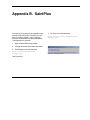
Appendix B. SaintPlus . . . . . . . . . . . . . . . . . . . . . . . . . . . . . . . . . . . . . . . . . . . . . .B-1
Appendix C. Using CELL_NOW . . . . . . . . . . . . . . . . . . . . . . . . . . . . . . . . . . . . . .C-1
C.1 Running CELL_NOW . . . . . . . . . . . . . . . . . . . . . . . . . . . . . . . . . . . . . . . . . . . . . . . . . . . . . . . C-1
C.2 CELL_NOW Output. . . . . . . . . . . . . . . . . . . . . . . . . . . . . . . . . . . . . . . . . . . . . . . . . . . . . . . . . C-9
Appendix D. Processing Twinned Data . . . . . . . . . . . . . . . . . . . . . . . . . . . . . . . .D-1
D.1 Integration with SAINTPLUS . . . . . . . . . . . . . . . . . . . . . . . . . . . . . . . . . . . . . . . . . . . . . . . . . . D-1
D.2 Scaling with TWINABS . . . . . . . . . . . . . . . . . . . . . . . . . . . . . . . . . . . . . . . . . . . . . . . . . . . . . . D-2
Appendix E. Config . . . . . . . . . . . . . . . . . . . . . . . . . . . . . . . . . . . . . . . . . . . . . . . . E-1
4
M86-E00078
1. Introduction
1.1 APEX II Systems for Chemical
Crystallography
controls all other aspects of the experiment,
from data collection through report generation.
Bruker AXS Kappa APEX II and SMART APEX
II systems are the newest members in the
Bruker Nonius product line of instrumentation
for single crystal X-ray diffraction. These systems provide the tools for complete small molecule structure determination. The hardware and
software are completely redesigned. The software features a new start-to-finish graphical
user interface (GUI). The hardware features a
new CCD detector based upon four-port readout
of a 4K chip and a choice of two goniometers.
APEX II systems are enclosed in a radiation
safety enclosure system.
The SMART APEX II system is an enhanced
version of the SMART APEX fixed-chi system. A
single computer controls the data collection, and
solution and refinement of the structure.
The Kappa APEX II system features the Kappa
4-axis goniometer. Two computers are used for
experiments. One computer, the server, controls
the goniometer. The other computer, the client,
M86-E00078
From a software and operational viewpoint, the
APEX II systems use the GUI of the APEX2
software suite to control all operations from
crystal screening to report generation for a typical crystallography study. This is a complete
departure from the command-driven, functionally separate modules of SMART, SAINTPLUS
and SHELXTL. Enhanced versions of the
proven and widely accepted programs used by
these modules (e.g., SAINT, SADABS, XPREP,
XS, XM, XL, etc.) underlie the GUI and provide
powerful tools.
1-1
Introduction
From a hardware viewpoint, APEX II systems
share common hardware components with other
Bruker products. Other members of this new
generation of instruments include the D8
ADVANCE and D8 DISCOVER, and the D8
GADDS systems for general diffraction. Documentation on some of these common hardware
and software components is available in the
user manuals for the D8 family of instruments.
APEX2 User Manual
1.2 User Manual Features
This user manual and associated YLID test data
are intended to provide you with a step-by-step
guide to data collection and processing using
the APEX2 software program.
The test data supplied was collected on a
Kappa APEX II diffractometer with graphite
monochromated molybdenum radiation from a
sealed tube generator. The high quality data
(resolution=0.75 Å) allows easy refinement of
the hydrogen atom positions and determination
of the absolute structure of the sample.
NOTE: Before using this manual, check that
your system is in proper working order (e.g., the
optics and goniometer are aligned) and that the
APEX2 suite is properly installed.
1-2
M86-E00078
APEX2 User Manual
Introduction
1.3 X-ray Safety
X-ray equipment produces potentially harmful
radiation and can be dangerous to anyone in the
immediate vicinity unless safety precautions are
completely understood and implemented. All
persons designated to operate or perform
maintenance on this equipment need to be fully
trained on the nature of radiation, X-ray
generating equipment and radiation safety. All
users of the X-ray equipment are required to
accurately monitor X-ray exposure by proper
use of X-ray dosimeters.
For safety issues related to the operation and
maintenance of your particular X-ray generator,
diffractometer and shield enclosure, please refer
to the manufacturer’s operation manuals or your
Radiation Protection Supervisor. The user is
responsible for compliance with local safety regulations.
M86-E00078
1-3
Introduction
1-4
APEX2 User Manual
M86-E00078
2. Hardware Overview
The two hardware platforms for the APEX II systems are the Kappa APEX II (the four-axis
advanced research instrument) and the SMART
APEX II (the three-axis laboratory instrument).
Software functionality is essentially the same for
both platforms.
M86-E00078
2.1 System Components
The system (Figure 2.1 and Figure 2.2) consists
of the following basic components.
•
APEX II CCD detector
•
4-axis Kappa or 3-axis SMART goniometer
•
K780 X-ray generator
•
Radiation safety enclosure with interlocks
and warning lights
•
D8 controller
•
Refrigerated recirculator for the detector
•
Computer(s) (two for the Kappa APEX II
and one for the SMART APEX II)
•
Video microscope
•
Accessories (high- and low-temperature
devices)
2-1
Hardware Overview
Figure 2.1 - Kappa APEX II system
2-2
APEX2 User Manual
Figure 2.2 - SMART APEX II system
M86-E00078
APEX2 User Manual
Hardware Overview
2.1.1 APEX II Detector
2.1.2 Goniometer
The APEX II detector is specific to this system.
Status lamps on the top of the detector housing
indicate when the detector is on (green) and off
(red).
The goniometer module and APEX II detector
make up the unique hardware of the system.
This is the part of the instrument that actually
performs the experiment.
On Kappa APEX II systems, the detector is
mounted on a motorized 2-theta track. The camera distance is computer-controlled (a typical
distance for the camera is 40 or 50 mm).
Several components make up the goniometer
module with APEX II detector:
On SMART APEX II systems, the detector is
mounted on a 2θ dovetail track. The track has a
scale that is calibrated in mm to indicate the distance from the crystal to the phosphor window
(a typical distance for the camera is 40 or 50
mm).
An optional motorized DX track is available for
the SMART APEX II.
M86-E00078
•
Goniometer (3-axis or 4-axis)
•
APEX II detector
•
X-ray source (including shielded X-ray tube,
X-ray safety shutter, and graphite crystal
monochromator)
•
K780 X-ray generator
•
Timing shutter and incident beam collimator
(with beamstop)
•
Video camera
2-3
Hardware Overview
APEX2 User Manual
Kappa APEX II Goniometer
The Kappa goniometer uses a horizontally oriented Kappa goniometer with 2-theta, omega,
kappa and phi drives and a motorized DX track
for setting the detector distance. It includes
mounting points for the video camera and for
optional attachments such as the optional low
temperature attachment.
Timing
Shutter
Sealed X-ray
Tube
Safety
Shutter
Incident
Beam
Collimator
Beamstop
Goniometer
Head
APEX II
Detector
Monochromator
Kappa
Stage
Kappa
Goniometer
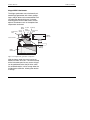
Figure 2.3 - Kappa 4-axis goniometer components
With the kappa angle, the crystal can be oriented at chi from -92° to 92°. This leaves the top
of the instrument open for easy access. Kappa
can be positioned so that the phi drive, which
has unlimited rotation, can be swung under the
incident beam collimator, allowing free rotation
in omega.
2-4
M86-E00078
APEX2 User Manual
Hardware Overview
SMART APEX II Goniometer
The SMART APEX II system uses a horizontally
oriented D8 goniometer base with 2-theta,
omega and phi drives, dovetail tracks for the Xray source and detector, and an additional
mounting track for accessories such as the
video camera and optional low-temperature
attachment.
The 3-axis system incorporates a fixed-chi
stage with chi angle of approximately 54.74°
and a phi drive with 360° rotation, which is so
compact that it swings under the incident beam
collimator, allowing free rotation in omega.
Beamstop
Fixed Chi Goniometer
Stage
Head
Rotary
Incident
Shutter and
Beam
Attenuator
Collimator Assembly
APEX II
Detector
Safety
Shutter
Sealed X-ray
Tube
Monochromator
D8
Goniometer
Figure 2.4 - SMART goniometer components
M86-E00078
2-5
Hardware Overview
X-ray Source
Three components make up the X-ray source: a
shielded X-ray tube, an X-ray safety shutter, and
a graphite crystal monochromator.
The sealed tube X-ray source, with a molybdenum (Mo) target, produces the X-ray beam used
by the system.
The X-ray safety shutter is built into the X-ray
tube shield. The shutter opens upon initiation of
a set of exposures and closes upon the end of
collection. Status lamps on the shutter housing
indicate when the shutter is open (red) or closed
(green). The shutter is also interfaced to the
controller and to the safety interlocks.
A tunable graphite crystal monochromator
selects only the Kα line (λ=0.71073 Å) emitted
from the Mo X-ray source and passes it down
the collimator system.
APEX2 User Manual
Because the generator is interfaced to the controller, the power settings can be adjusted within
the APEX2 software. This is usually not necessary as the software automatically increases the
power to the user-defined values at the beginning of an experiment and lowers them when
the instrument is inactive.
Timing Shutter and Collimator
On SMART APEX II systems, the monochromatic X-ray beam then passes through the labyrinth, the timing shutter, and the incident beam
collimator before striking the specimen. On
Kappa APEX II systems, the monochromatic Xray beam passes through a small labyrinth, the
timing shutter, a secondary labyrinth and the
incident beam collimator before striking the
sample.
•
The labyrinth is a device that ensures that
the collimator and shutter are tightly connected to prevent X-ray leakage.
•
The timing shutter is a device which precisely controls the exposure time for each
frame during data collection. Its status
lamps indicate when the shutter is open
(ON) and closed (OFF). For SMART APEX
II systems, this assembly also houses an
automatic attenuator. Kappa APEX II systems do not have an attenuator.
•
The incident beam collimator is equipped
with pinholes in both the front (near crystal)
and rear (near source). These pinholes help
K780 X-ray Generator
The K780 X-ray generator is a high-frequency,
solid-state X-ray generator that provides a stable source of power for operations up to 60 kilovolts (kV) and 50 milliamps (mA).
Typical maximum power settings for the APEX II
system with a fine focus tube are 50 kV, 40 mA.
Either copper or molybdenum tubes may be
used on APEX II systems. For both types of
tubes, the kV setting should not exceed 50 kV
and the power (kV x mA) should not exceed the
power rating given on the tube cap.
2-6
M86-E00078
APEX2 User Manual
to define the size and shape of the incident
X-ray beam that strikes the specimen. (Collimators are available in a variety of sizes,
depending on your application.)
•
The beamstop catches the remainder of the
direct beam after it has passed the specimen. The beamstop has been aligned to
minimize scattered X-rays and to prevent
the direct beam from hitting the detector.
The entire collimator assembly is supported
by a collimator support assembly, which has
been precisely aligned to guarantee that the
X-ray beam passes through the center of
the goniometer.
Video Camera
The video camera, an essential part of the system, allows you to visualize the crystal to optically align it in the X-ray beam. It also allows you
to measure the crystal’s dimensions and index
crystal faces. The camera is interfaced to the
computer and is operated through the VIDEO
program. The VIDEO program includes several
computer-generated reticles and scales to make
it easy to center and measure the crystal.
M86-E00078
Hardware Overview
2.1.3 Radiation Safety Enclosure with
Interlocks and Warning Lights
A common component of all systems in the D8
family is the radiation safety enclosure. This
new design is fully leaded (i.e., leaded windows,
leaded metal sides and panels) to protect you
from stray radiation. The enclosure also
includes warning lamps (a government requirement) that alert you when X-rays are being generated. As a special feature, the enclosure also
incorporates interlocks for both hardware and
software: an automatic system-interruption
device that senses when the doors and panels
are open and prevents data collection and use
of the shutter until you close the doors.
2.1.4 D8 Controller
The D8 controller is an electronic module
enclosed in the rack behind the front panel of
the instrument. It contains all of the electronics
and firmware for controlling the generator, opening the X-ray shutters, and monitoring other
instrument functions such as safety interlocks,
generator status, and detector status. For
SMART APEX II systems, the goniometer is
controlled by the D8 controller. For Kappa APEX
II systems, there is an additional module, the
Kappa controller, for positioning the Kappa goniometer angles and adjusting the detector distance by driving the detector along its track.
2-7
Hardware Overview
2.1.5 Refrigerated Recirculator for the
Detector
To minimize dark current in the APEX II detector, dual Peltier devices are used to cool the
CCD chip to approximately -58°F (-50°C). The
refrigerated recirculator uses an ethylene glycol/
water mixture to absorb the heat from the Peltier
devices.
APEX2 User Manual
2.1.7 Accessories
Various devices can be mounted on the goniometer base. These include optional low- and hightemperature attachments. Both instruments can
be used with diamond-anvil cells.
2.1.6 Computer(s)
The Kappa APEX II system uses two highspeed computers. The server controls the
instrument and is used for crystal centering and
screening. The client collects the data, stores
the raw frames, processes the data, and solves
and refines the structure. The two computers
are linked via a hub and communicate with each
other via TCP/IP protocols.
The SMART APEX II system uses a single highspeed computer for control of the experiment,
storage of raw frame data, integration of the
data, and solution and refinement of the structure.
The computer or computers are often attached
to a network of similarly configured computers
with access to local and/or network printers.
NOTE: Connection to the external network must
be done with care. Consult with local security
experts.
2-8
M86-E00078
3. Software Overview
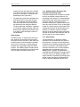
This section presents an outline of the system
software, including a brief description of the software layout as well as the graphical user interface (GUI).
APEX2 runs on two computers: the server and
the client. For SMART APEX II systems, the
server and the client execute on the same computer, but their functionality remains separate.
The flowchart in Figure 3.1 shows the software
layout. For both Kappa APEX II and SMART
APEX II systems, the server and client communicate using TCP/IP protocol.
Figure 3.1 - APEX2 software diagram
M86-E00078
3-1
Software Overview
APEX2 User Manual
3.1 The Server Computer
3.1.2 Bruker Control Program (BCP)
The server computer communicates with the
hardware, allowing the user to control the instrument. The server computer runs software for
aligning the system, as well as software for
aligning and screening samples.
BCP is used to configure BIS, as well as to provide instrument control and alignment tools. See
the online help within BCP for more information.
3.1.1 Bruker Instrument Service (BIS)
BIS provides the link between the hardware and
software. Once a connection is established, BIS
executes hardware commands sent by the
APEX2 software. The instrument service can
also be used as a service tool, displaying diagnostic messages during operation.
Figure 3.2 - BCP main window
3-2
M86-E00078
APEX2 User Manual
Software Overview
3.1.3 APEX2 Server
The APEX2 Server provides tools for aligning
and screening samples. There are two main
items: Align Crystal and Simple Scans (see Figure 3.3).
Figure 3.3 - Simple Scans window
M86-E00078
3-3
Software Overview
APEX2 User Manual
3.2 The Client Computer
The client can be any computer on the same
network as the server. For SMART APEX II systems, it is usually the same computer as the
server. The main portion of the APEX2 suite, the
APEX2 client, runs on the client computer. The
client is a GUI with multiple plug-ins or modules
for different aspects of an experiment. The client
includes a database which stores relevant data
from each step in the experiment. Details of the
functions available in the GUI will be explained
in more detail later in the manual.
3.2.1 Database and Database Connection
As currently configured, the database is used
internally by the APEX2 Suite and is not available for user customization or manipulation. It
must be running before the APEX2 Suite is
started and it should be stopped before the
computer is shut down (see Section 4.3.2).
The database is used for the storage of data
generated by the Bruker APEX2 software.
3-4
M86-E00078
APEX2 User Manual
Software Overview
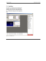
3.2.2 APEX2 GUI
•
Window Tool Bar
The APEX2 GUI has one main window (see Figure 3.4). This window is divided into four sections:
•
Tool Icon Bar
•
Task Bar
•
Task Display Area
Window Tool Bar
Tool Icon Bar
Task
Bar
Task Display
Area
Figure 3.4 - APEX2 GUI
M86-E00078
3-5
Software Overview
APEX2 User Manual
Window Tool Bar
Tool Icon Bar
The tool bar provides pull-down menus for a
variety of file operations, image tools, and help
files.
The tool icon bar provides shortcuts to the
options available through the window tool bar.
Option
Description
[Symbol]
Use this menu to select the following:
Restore, Move, Size, Minimize, Maximize, and Close.
File
Use this menu to select the following:
Login, Logout, New, Open, Save, Close,
Import (Spatial), Export (.p4p file) and
Exit.
Instrument
Use this menu to select the following:
Connection, Status, Toggle Shutter and
Abort.
Windows
Use this menu to select the following:
Cascade and Tile.
RLATT
(available when
you select
Reciprocal
Lattice Viewer)
Use this menu to select the following:
Rotate, Edit, Orientation, Unit Cell Tool,
Measure Distance, Measure Angle and
Visualization.
View
Use this menu to select the following:
(available when Detailed Strategy.
you select Data
Collection
Strategy)
Icon
Description
Create a new file.
Open a file.
Save a file.
“What’s this?” Context-sensitive help.
Open an image.
Select the first image in a run. This icon is visible only when an image is displayed.
Table 3.1 – Window tool bar options
Select previous image. This icon is visible
only when an image is displayed.
Table 3.2 – Tool icon bar options
3-6
M86-E00078
APEX2 User Manual
Icon
Description
Select next image. This icon is visible only
when an image is displayed.
Software Overview
Icon
Description
Select a region of the image. This icon is visible only when an image is displayed.
Table 3.2 – Tool icon bar options
Select the last image in a run. This icon is visible only when an image is displayed.
Go down one run.
Go up one run.
Draw a resolution circle. This icon is visible
only when an image is displayed.
Draw a plotting line. This icon is visible only
when an image is displayed.
Change the part of the image displayed while
zoomed in. This icon is visible only when an
image is displayed.
Table 3.2 – Tool icon bar options
M86-E00078
3-7
Software Overview
Task Bar
APEX2 User Manual
Collect
The task bar provides menus for all of the
options in the APEX2 Suite: crystal evaluation
and indexing (Evaluate Crystal), data collection
(Collect), data processing (Integrate and Scale),
and instrument setup (Instrument).
Data Collection Strategy - Simulated data
collection and determination strategy.
Setup
Experiment - Sequence editor for data collection experiments.
Describe - Specify crystal size, color,
shape, etc.
Oriented Scans - Measure different images
with the crystal aligned along the axes.
Center - Perform crystal centering functions.
Integrate
Evaluate Crystal
Integrate Images - Integration of different
data.
Determine Unit Cell - Determine unit cell
and Bravais lattice type.
Scale
Reciprocal Lattice Viewer - 3D visualization
of lattice projected in reciprocal space.
Scale - Scale intensities and perform
absorption correction.
View Images - View collected frames.
Table 3.3 – Task bar options
3-8
Table 3.3 – Task bar options
M86-E00078
APEX2 User Manual
Software Overview
Examine Data
XPREP (Space Group Determination) Run XPREP.
Precession Images - Create synthesized
precession images based on measured
frames.
Solve Structure
Structure Solution - Solve the phase problem to get an initial model.
Refine Structure
Structure Refinement - Use least squares
to improve the model.
Report
Run XCIF to generate a report.
Table 3.3 – Task bar options
M86-E00078
3-9
Software Overview
APEX2 User Manual
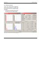
Task Display Area
The Task Display area is the main area for
tasks, user input, and selected output. This area
displays images, the reflections used in indexing, and the observed and predicted diffraction
patterns. It also displays the runs for data collection and solution and refinement. (For version
1.22,
space group determination, SaintChart output,
XSHELL refinement, and XCIF report generation do not use the Task Display Area; they
open in a new window). All other plug-ins open
in the Task Display area of the GUI.
Figure 3.5 - The Task Display area showing COSMO
3 - 10
M86-E00078
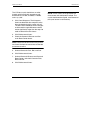
4. Program Start-Up and Shutdown
As mentioned previously, the APEX2 Suite is
composed of several programs. All of the programs are started in a similar fashion. For ease
of use there is usually a desktop icon for the
folder containing these programs, and desktop
icons linked directly to these programs. However, the Start > Programs > Bruker … path is
always available. This more explicit method will
be used in this discussion.
4.1 Server Computer Start-Up
Two programs must be running: Bruker Instrument Service and APEX2 Server.
NOTE: For Kappa APEX II systems, the programs will be on the server computer in the
goniometer cabinet. For SMART APEX II systems, there is typically only one computer.
4.1.1 Starting Bruker Instrument Service
(BIS)
1. Click on Start > Programs > Bruker AXS
Programs > Bruker Instrument Service or
click on the BIS icon on the desktop.
M86-E00078
4-1
Program Start-Up and Shutdown
After a brief initialization period, a window will
appear (see Figure 4.1). On Kappa APEX II systems, the goniometer will move to reference
positions.
APEX2 User Manual
NOTE: With a Kappa APEX II, the kappa goniometer will home and the kappa server will activate when BIS is started. This may take a
minute or two. The Kappa server is a service
tool and should not be used to control the instrument.
Figure 4.1 - The BIS window
If a small pop-up window appears that says
“This second instance of BIS is exiting” (see Figure 4.2), BIS was already running. Click on OK
to clear this informational message.
Figure 4.2 - BIS exiting message
4-2
M86-E00078
APEX2 User Manual
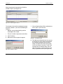
4.1.2 Starting the APEX2 Server
1. Click on Start > Programs > Bruker Nonius
Programs > APEX2 Server or click on the
APEX2 Server icon on the desktop.
Program Start-Up and Shutdown
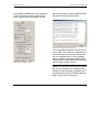
2. In the top left corner, click on the Instrument
pull-down menu (see Figure 4.4).
A window will appear (see Figure 4.3).
Figure 4.4 - Connecting to the instrument
3. Click on Connection and a new window will
appear (see Figure 4.5). The name of your
server should already be filled in.
4. Click on Connect.
Figure 4.3 - Initial APEX2 Server window
Figure 4.5 - Connection window
NOTE: If the host name is wrong, then the
instrument is not properly configured and you
should consult your system manager. (It is possible to configure the instrument to automatically
connect so that this window will not appear).
This is discussed in Appendix E: Config.
M86-E00078
4-3
Program Start-Up and Shutdown
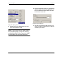
4.2 Client Computer Start-Up
On the client computer, two programs are also
required: the database and APEX2. It is best to
start the database before starting APEX2.
APEX2 User Manual
You can minimize this window. If the database
has not previously been closed properly (e.g.,
after a power failure), a window will appear (see
Figure 4.7) that states that another postmaster
is running. If this happens, stop the database
and then start it again.
NOTE: For the SMART APEX II, there is typically only one computer for the client and server
software.
4.2.1 Starting the Database
1a. For Windows systems, click on Start > Programs > Bruker AXS Programs > Start
Database or click on the Start Database
icon on the desktop.
Figure 4.7 - Database failure message
4.2.2 Starting APEX2
1a. For Windows systems, on the client computer click on Start > Programs > Bruker
Nonius Programs > APEX2 or click on the
APEX2 icon on the desktop.
1b. For Linux systems, open a terminal window
and type
bnrun startdb
or click on the Start Database icon.
A window should appear that says the database
system is ready.
1b. For Linux systems, open a terminal window
and type
bnrun apex2
or click on the APEX2 icon.
Figure 4.6 - The database is ready
4-4
M86-E00078
APEX2 User Manual
2. A window will prompt you to log in to the
database by entering a user name and
password (see Figure 4.8).
Program Start-Up and Shutdown
4. Click on File.
2.1 If the system manager has set up the
system to automatically enter the user
name and password, step 2 is skipped.
Figure 4.10 - File menu
5. Use the options in this menu to create a
new project or to open an existing project.
Figure 4.8 - Login request
6. If the window in Figure 4.11 appears, then
APEX2 thinks the database is already in
use. Answer “Yes” to close the window.
3. An empty start-up window will appear (see
Figure 4.9).
Figure 4.11 - Sample locked window
Figure 4.9 - APEX2 start-up window
M86-E00078
4-5
Program Start-Up and Shutdown
4.3 Client Computer Shutdown
APEX2 User Manual
A window will appear and quickly disappear, and
the Start Database window will close.
NOTE: The order of stopping these programs is
important. If you attempt to close the database
before APEX2 is stopped, the database will
remain open until APEX2 is stopped.
4.3.1 Stopping APEX2
1. For Windows or Linux systems, click on the
X in the upper right corner of the window or
click on File > Exit in the upper left. It is not
necessary to disconnect from the instrument.
4.3.2 Stopping the Database
1a. For Windows systems, click on Start > Programs > Bruker Nonius Programs > Stop
Database or click on the Stop Database
icon.
Figure 4.12 - Stop database screen
NOTE: Occasionally the windows won’t disappear and the Start Database window will display
a “smart shutdown request” (see Figure 4.12).
This message means that the database is waiting to close until applications that it might write
to are closed. Exit APEX2 to solve this problem.
If the message still appears, use the Task Manager to check for other processes that may still
be running (e.g., COSMO).
1b. For Linux systems, in a terminal window
enter
bnrun stopdb
or click on the Stop Database icon.
4-6
M86-E00078
APEX2 User Manual
Program Start-Up and Shutdown
4.4 Server Computer Shutdown
Stop APEX2 Server before BIS. It is acceptable for the order to be reversed. Generally, BIS
is never stopped.
4.4.1 Stopping the APEX2 Server
1. Click on the X in the upper right corner of
the window or click on File > Exit in the
upper left. It is not necessary to disconnect
from the instrument.
4.4.2 Stopping BIS
It is almost never necessary to stop and exit
BIS. If necessary, click on the Stop BIS button
on the bottom of the BIS window and then click
on the Exit button at the bottom of the window.
M86-E00078
4-7
Program Start-Up and Shutdown
4-8
APEX2 User Manual
M86-E00078
5. Crystal Orientation
We are now ready to begin data collection with
the instrument. It is assumed that your system
manager has set up the system properly and
that all system default parameters have been
set appropriately.
The data collection process is divided into five
steps, which will be covered in Section 5 and
Section 6. The steps in Section 5 are performed
using the APEX2 Server software on the server
computer. The steps in Section 6 are performed
using the APEX2 program on the client computer.
See Section 5 for:
2. Crystal quality check (from the APEX2
Server—the Simple Scans module)
See Section 6 for:
3. Cell determination (from APEX2—the Cell
Determination module)
4. Data collection setup (from APEX2—the
Strategy module)
5. Data collection (from APEX2—the Experiment module)
The first steps—mounting, aligning and screening a crystal—are performed on the server computer.
1. Centering/aligning the crystal on the diffractometer (from the APEX2 Server—the Center module)
M86-E00078
5-1
Crystal Orientation
5.1 Mount the Goniometer Head on
the Instrument
1. Open the enclosure doors. Push either of
the rectangular green Open Door buttons on
the side posts. This will release the door
locks for approximately five seconds. During
this time, pull out on one or both of the handles to physically open the doors.
2. In the APEX2 Server GUI, under Setup click
on Center Crystal.
The centering buttons will appear and the video
window will open.
APEX2 User Manual
The bottom five buttons will drive the goniometer to various pre-defined positions that are
designed to simplify crystal centering. The top
two buttons will drive phi by either 90 or 180
degrees.
3. Click on Mount to mount the goniometer
head.
4. Carefully remove the goniometer head containing the crystal from its case.
Use extreme care when handling the
goniometer head to prevent damage to the
sample on the end of the small glass fiber.
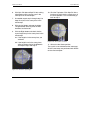
5. Place the goniometer head onto its base on
the phi drive. Line up the slot on the bottom
of the goniometer head with the pin on the
mounting base (see Figure 5.2).
Figure 5.1 - The Center buttons
Figure 5.2 - View of the bottom of the goniometer head
5-2
M86-E00078
APEX2 User Manual
Crystal Orientation
6. Screw the head’s collar to the base so that
the head does not move. Do not overtighten
it (finger-tighten only).
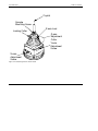
Figure 5.3 - Huber goniometer head in detail
M86-E00078
5-3
Crystal Orientation
APEX2 User Manual
#RYSTAL
3AMPLE
-OUNTING3CREW
,OCKING#OLLAR
:AXIS,OCK
:AXIS
!DJUSTMENT
#OLLAR
9AXIS
!DJUSTMENT
3CREW
8AXIS
!DJUSTMENT
3CREW
Figure 5.4 - Standard goniometer head in detail
5-4
M86-E00078
APEX2 User Manual
5.2 Center and Align the Sample
To obtain accurate unit cell dimensions and to
collect good quality data, align the center of the
sample with the center of the X-ray beam and
maintain this alignment for the entire experiment. Your video camera should be aligned so
that the crosshairs of the video camera coincide
with the center of the goniometer and the center
of the X-ray beam (see manual M86-Exx024 for
instructions on aligning the microscope to the
center of the instrument). If the microscope is
not centered, you can still align the sample—the
key to crystal centering is that the crystal stays
in the same place in the microscope’s field of
view in all orientations.
NOTE: Use the thin end on the goniometer
wrench to unlock the X, Y and Z locks at the
beginning of the centering process and to lock
them at the end—locking needs only a very
slight touch. The other end of the wrench is
used to move the adjustment slides. Do not
overtighten.
Crystal Orientation
NOTE: Centering is often easier if the crystal is
rotated to give a good view before the actual
centering process is started (e.g., down an edge
for a plate). To do this, drive to one of the centering positions, loosen the screw that locks the
crystal mounting pin, rotate the crystal to a suitable orientation and then tighten the screw
again.
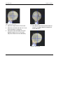
5.2.1 For a Kappa APEX II System
1. Click the Center button—the crystal and
goniometer head will be positioned perpendicular to the microscope. To center the
sample, make adjustments in the height
with the Z-axis adjustment and with the
translation screw that faces the front of the
diffractometer.
Figure 5.5 - Crystal initially mounted
M86-E00078
5-5
Crystal Orientation
APEX2 User Manual
Figure 5.6 - Crystal centered
Figure 5.7 - Spin Phi 90
2. Adjust the height with the Z-axis screw.
5. Click Spin Phi 180 and adjust the screw facing you, as needed. (Adjust to remove half
of the difference.)
3. Adjust the translation with the X- or Y-axis
screw, whichever is facing you.
4. Click Spin Phi 90 and adjust the crystal
position using the X- or Y-axis screw.
(Adjust to remove half of the difference.)
Figure 5.8 - Spin Phi 180
5-6
M86-E00078
APEX2 User Manual
6. Click Spin Phi 180 and Spin Phi 90, making
adjustments until the crystal stays in the
same place in the microscope.
7. As needed, repeat step 2 through step 5 to
keep the crystal in the same place in the
microscope.
Crystal Orientation
10. Click the Top button. Click Spin Phi 180 a
few times to verify that the sample stays in
the same position. If it is not centered, go
back to step 2.
8. Click the Left button and note the height.
The goniometer drives to place the fiber
horizontal and to the left.
9. Click the Right button and check that the
crystal height stays in the same place in the
microscope.
9.a If the height is in the same place, you
are done.
9.b If the height is not in the same place,
adjust to remove half of the difference
and repeat step 8 and step 9.
Figure 5.10 - The crystal is centered
11. Go back to the Center position.
The crystal is now centered on the instrument.
All of the next steps are performed with APEX2
on the client computer.
Figure 5.9 - Check the crystal height
M86-E00078
5-7
Crystal Orientation
APEX2 User Manual
5.2.2 For a SMART APEX II System
NOTE: If the image of the crystal is difficult to
see, illuminate the sample with a high-intensity
lamp and/or temporarily place a light-colored
piece of paper on the front of the detector.
1. Click the Right button. The crystal and goniometer head will be positioned perpendicular to the microscope. To center the sample,
make adjustments to the height with the Zaxis adjustment.
Figure 5.12 - Initial center position
Figure 5.13 - Initial X- or Y-axis (translation) ajustment
Figure 5.11 - Initial mounted crystal
3. Click Spin Phi 90. Remove half of the difference with the adjustment screw that is facing you.
2. Click the Center button. Move the crystal so
that it is centered in the microscope reticle
by adjusting the X- or Y- axis translation
adjustment screw that is perpendicular to
the microscope axis and facing you (see
Figure 5.3 and Figure 5.4).
Figure 5.14 - Spin Phi 90
5-8
M86-E00078
APEX2 User Manual
Crystal Orientation
4. Click Spin Phi 180. Remove half of the difference with the adjustment screw that is
facing you.
5. Click Spin Phi 180 again.
5.1 If the crystal is centered, click Spin Phi
90.
5.2 If the crystal is not centered, adjust to
remove half of the difference and click
Spin Phi 180. Repeat until the crystal is
centered. Click Spin Phi 90.
5.3 If centered, adjust the height. If not centered, repeat steps 2 through 5 until it is
centered.
Figure 5.16 - Check Left
7. Click the Right button. Adjust the height.
Adjust to remove half of the difference.
Figure 5.17 - Check Right
Figure 5.15 - Height adjusted
6. Click the Left button. Adjust to remove half
of the difference. Adjust the height.
8. If a height adjustment was made in step 6 or
7, repeat those steps to check the height. If
the height is adjusted, repeat steps 2 to 5 to
check the centering. If no height adjustment
was made, the crystal is centered.
The crystal is now centered on the instrument.
All of the next steps are performed with APEX2
on the client computer.
M86-E00078
5-9
Crystal Orientation
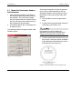
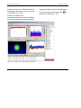
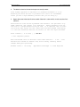
APEX2 User Manual
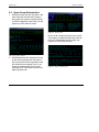
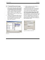
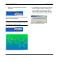
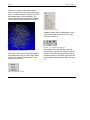
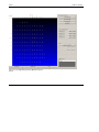
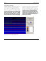
5.3 Simple Scans
The Simple Scan plug-in provides the tools for
rapid screening of the sample to check sample
quality. It allows the user to quickly set up scans
to measure a 360-degree phi rotation as well as
still, thin (0.5 degree) and thick (2.0 degree)
images.
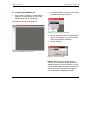
1. Click on the Simple Scan icon. The menu
shown in Figure 5.18 will open.
Figure 5.18 - Simple Scans menu
5 - 10
M86-E00078
APEX2 User Manual
The sliders and data boxes at the top can be
used to position the detector.
The buttons in the middle provide easy access
to common movements.
There are four possible user-defined buttons.
The Drive button initiates the requested movement. If it is gray, an impossible movement has
been requested.
The buttons and boxes at the bottom set up
scans. In Figure 5.18, the Drive + Scan button is
grey and therefore inactive because no scan
has been requested.
Crystal Orientation
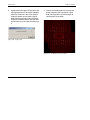
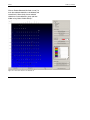
4. Click 360degree Phi and set the desired
exposure time. The default of 15 seconds is
usually sufficient.
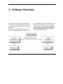
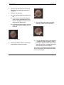
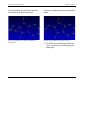
5. Click “Drive + Scan”. Since these are evaluation scans, there is no need to request correlated images or new darks. The resulting
Phi 360° image is shown in Figure 5.19. The
crystal diffracts nicely with lots of sharp
spots. Figure 5.23 shows a Phi 360° scan
with a bad crystal.
2. Click on Zero and then on Drive.
3. Set the distance.
3.1 On Kappa APEX II systems, check that
the moveable beamstop is pushed in
and set the desired position (typically
45 mm) for Distance in the data window.
3.2 On SMART APEX II systems with movable DX, set the desired position (typically 50 mm) for Distance in the data
window.
3.3 On SMART APEX II systems with fixed
DX, check that the distance displayed is
the same as the actual distance in mm
on the detector arm.
M86-E00078
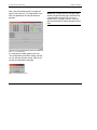
Figure 5.19 - A 360° Phi scan on a good quality crystal
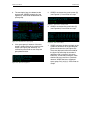
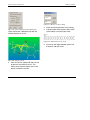
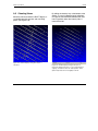
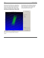
6. Click on Wide (2.0), change the scan range
to 2.0 and set the desired exposure time. A
time of 5 to 15 seconds is usually sufficient.
5 - 11
Crystal Orientation
APEX2 User Manual
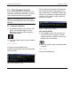
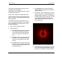
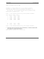
7. Click “Drive + Scan”. The resulting 2-degree
scan is shown in Figure 5.20. The spots are
sharp and clean. There are no peaks that
are very close together. Figure 5.24 shows
a 2-degree scan with a bad crystal.
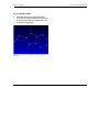
Figure 5.21 - A 2° phi scan at plus 90 in phi on a high quality
crystal. The spots’ shapes are well-defined and the spots
are well-separated.
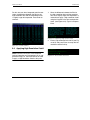
10. Set 2Theta to -30. This will allow evaluation
of the diffraction at higher angles.
Figure 5.20 - A 2° phi scan on a high quality crystal. The
spots’ shapes are well-defined and the spots are wellseparated.
8. Click “Phi + 90” in the middle row of boxes.
9. Click “Drive + Scan”. The resulting 2-degree
scan is shown in Figure 5.21. This image is
measured 90 degrees from the previous
one giving a view of the diffraction pattern
from a different (perpendicular) direction.
Figure 5.25 gives a similar view for the poor
crystal.
5 - 12
M86-E00078
APEX2 User Manual
Crystal Orientation
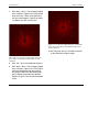
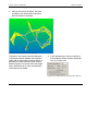
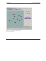
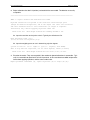
11. Click “Drive + Scan.” The resulting image is
shown in Figure 5.22.
Figure 5.22 - A 2° phi scan on a high quality crystal at 2theta of -30. The cursor is pointing to an area between the
two reflections shown in the 2D box. The cursor info at the
bottom left shows the resolution is 0.93 and 2-theta is 45.
M86-E00078
5 - 13
Crystal Orientation
APEX2 User Manual
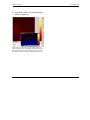
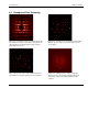
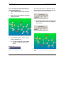
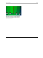
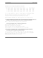
5.4 Examples of Poor Screening
Figure 5.23 - A 360° phi scan on a poor quality crystal. The
spot shape is poor and the spots tend to run together. The
obvious bands on the image suggest that the crystal is
nearly aligned on an axis.
Figure 5.25 - A 2° phi scan on a poor quality crystal at plus
90 in phi. The spot shape is poor and the spots are very
close together.
Figure 5.24 - A 2° phi scan on a poor quality crystal. The
spot shape is poor and the spots are very close together.
Figure 5.26 - A 360° phi scan on a small crystal. The
diffraction power of the crystal is small, but with slower
scans this is clearly a reasonable candidate for data
collection.
5 - 14
M86-E00078
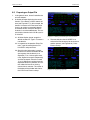
6. Data Collection
The data collection process is carried out on the
client computer using APEX2. Once data collection is started, exit APEX2 (optional). Data collection will continue regardless.
6.1 Start a New Project and
Describe the Sample
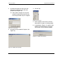
1. In APEX2, left-click on File > New.
2. In the window that appears, enter the sample name.
Figure 6.1 - The New Sample window
3. Click OK.
4. The task bar will appear with the Setup section open. Left-click on Describe.
M86-E00078
6-1
Data Collection
APEX2 User Manual
5. Enter the requested information into the
Describe window.
Figure 6.2 - Describe window
6. Close this module. The data will automatically save to the database.
6-2
M86-E00078
APEX2 User Manual
Data Collection
6.2 Determine the Unit Cell
6.2.1 Collect Images
1. In the task bar, left-click on Collect and then
Experiment.
If there was no connection to the instrument
when this module was started, the program will
either automatically connect or it will recognize
that it needs to connect in order to collect
images, and will ask to connect (see Figure 6.3).
Figure 6.3 - Instrument Connection window
2. Click on Connect.
3. Click on Append Matrix Strategy at the bottom left of the window.
M86-E00078
6-3
Data Collection
APEX2 User Manual
Figure 6.4 - Append matrix runs
4. Adjust the scan time and scan width if
desired. The default values are usually
good. The default time of 10 seconds works
for most samples, but shorter times will not
adversely affect most experiments.
5. Click on Execute. The view will shift to the
Monitor Experiment view (see Figure 6.5).
The program will collect a series of three
runs with twelve frames per run. This typically takes less than ten minutes. The
images will stop changing when the experiment is done. It is not necessary to wait for
all runs to complete before proceeding to
the harvesting step (step 6.2.2).
6-4
NOTE: Adjust the time (upper right) to match the
scattering ability of the crystal (i.e., shorter
exposure times for strong diffractors and longer
times for weak diffractors). If the exposure times
are five seconds or less, click on the check mark
by Correlate Frames to turn off this feature.
Frame correlation takes two exposures for each
frame, each typically having half the duration of
the full exposure, and then combines the two
together. This is usually not necessary with
shorter exposure times.
M86-E00078
APEX2 User Manual
Data Collection
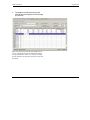
NOTE: The format for frame names is shown in
Figure 6.5. APEX2 assigns every frame a name.
For this figure, the name is
ylid_manual_01_005.sfrm. This means that the
frame is for the project ylid_manual and that this
is the fifth image of the first run.
Left and right
arrows move
between frames
Up and down
arrows move
between runs
Figure 6.5 - Monitor Experiment view
M86-E00078
6-5
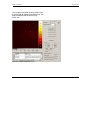
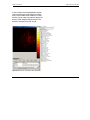
Data Collection
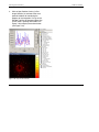
To change the color of the image display (e.g.,
Black On White), right-click in the intensity bar
to the right of the image display (see Figure 6.6).
APEX2 User Manual
6.2.2 Harvest the Reflections
1. Left-click on Evaluate Crystal > Determine
Unit Cell.
Figure 6.7 - The Determine Unit Cell (Indexing) icon
Figure 6.6 - Color tool
NOTE: After the first run is completed, there is
usually sufficient information to start the indexing step.
6-6
M86-E00078
APEX2 User Manual
Data Collection
This will open the image viewer, but with a tool
bar to the right for indexing (see Figure 6.8). The
plug-in initializes with the first run (e.g.,
matrix_01).
Figure 6.8 - Image viewer with indexing tool
M86-E00078
6-7
Data Collection
2. The name of the first image is already
entered. Click on Harvest Spots.
NOTE: All other options are gray at this point
because no reflections are available.
A blue progress bar will appear as the software
determines the best background level to use for
harvesting. Then a window with two sliders will
appear.
APEX2 User Manual
3. Change the run number in the “First Image”
box to matrix_02_0001 and click on Harvest
Spots. The run number is 02. The image or
frame number is 0001.
4. Change the run number in the “First Image”
box to matrix_03_0001 and click on Harvest
Spots.
At this point you should have 100 to 300 reflections harvested.
NOTE: If you have started harvesting before all
of the matrix runs were collected, a window may
pop up that says “Do you want to continue with
the images that could be read?” If this happens
and only one or two frames are needed to complete the run, wait, and then process the entire
run. However, if you have a hundred or more
spots and there are several frames yet to be collected, you can skip step 3 or 4 and go to Section 6.2.3. Then return to Section 6.2.2 and
harvest the spots before refining.
Figure 6.9 - Indexing sliders
The right slider selects which image is displayed. The left slider increases or decreases
the I/s(I), the cutoff criteria for accepting reflections. Generally, the defaults are acceptable.
6-8
M86-E00078
APEX2 User Manual
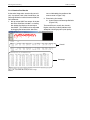
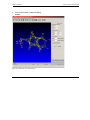
6.2.3 Index the Reflections
1. Click on Index in the tool bar to the right of
the image viewer. A window will open.
Data Collection
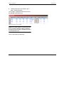
After approximately 30 seconds, the Index window will display a possible cell and the OK button will no longer be gray. The values shown in
Figure 6.11 are reasonable for the YLID crystal.
Figure 6.11 - The unit cell
The spot statistics are also acceptable with 98%
(i.e., (238/244)x100) of the selected spots
indexed.
Figure 6.10 - Indexing tool
The defaults are usually acceptable. Use the
slider to omit reflections with lower I/sigma from
the calculations. If indexing is difficult, try reducing the number of reflections used.
If indexing is difficult, use the RLATT tool. This
tool is described in Appendix A.
2. Click on Index.
Figure 6.12 - Focus on the spot results
There are often a few reflections that are not
indexed. You can use the reciprocal lattice
viewer to look at the spots used in the indexing,
but refine this cell first .
3. Click on OK to accept the indexing results.
M86-E00078
6-9
Data Collection
APEX2 User Manual
6.2.4 Refine the Unit Cell
There is not a correct order for the following
steps. Use this procedure as a guideline with
the main goal of creating a stable converged
refinement.
1. Click Refine in the Indexing Tools menu.
The Refine Unit Cell window will open.
Figure 6.13 - The Refine menu with histograms displayed
6 - 10
M86-E00078
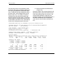
APEX2 User Manual
The YLID test crystal should have an orthorhombic primitive cell with approximate cell
dimensions of a=5.95Å, b=9.03Å, c=18.38Å,
and α=β=γ=90°.
2. Click View Histograms. The histograms
show how observed data compares to the
data calculated using the current unit cell.
The HKL values should be close to integers
and the rotation angle differences should
not be significantly larger than the step size
used to collect the matrix frames.
Data Collection
NOTE: In most cases, the angle zeroes are
close to zero and should not be refined. The
crystal should now be aligned, so refinement of
the crystal center is not necessary.
3. Click Refine several times.
4. Check the Constrain Distance and Constrain Beam Center boxes.
NOTE: Check the constraints to fix the parameters listed. Uncheck the constraints to allow the
parameters to refine.
5. Uncheck Constrain Pitch, Roll, and Yaw.
6. Click Refine several times.
7. Uncheck Constrain Distance and Constrain
Beam Center, and check Constrain Pitch,
Roll, and Yaw.
8. Click Refine several times.
M86-E00078
6 - 11
Data Collection
APEX2 User Manual
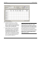
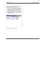
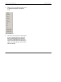
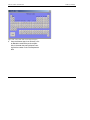
6.2.5 Determine the Bravais Lattice
1. After refining, click Bravais Lattice and look
for other unit cell choices (i.e., look at fit values).
Figure 6.14 - Bravais lattice display
Note that even though monoclinic has a slightly
better fit, the software makes the correct choice
of the higher symmetry cell.
Now you have a unit cell ready for determining a
data collection strategy.
2. Click on the appropriate Bravais lattice (in
this case, Orthorhombic).
3. Press OK to accept the suggested lattice
settings.
4. Refine again.
5. Refine for several more cycles, changing
the constraints one or two at a time.
6 - 12
M86-E00078
APEX2 User Manual
Data Collection
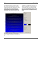
6.3 Determine the Data Collection
Strategy
APEX2 includes a powerful algorithm, COSMO,
for determining an efficient strategy that fully utilizes the flexibility of your instrument.
1. Left-click on Collect > Data Collection Strategy.
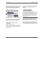
Figure 6.15 - The strategy display
M86-E00078
6 - 13
Data Collection
NOTE: COSMO will use information from cell
determination to set defaults. You can modify
the suggested values.
2. Check the inputs for defining the data collection.
2.1 Set the data collection distance. For
SMART APEX II systems, this should
be set to the actual detector distance.
For Kappa APEX II systems, there is a
variable (DX) and the distance will
default to the shortest reasonable distance. For the APEX II detector, the distance in millimeters should generally be
about the same as the longest cell
dimension in angstroms. Typically, distances ranging from 35 to 45 are reasonable.
2.2 Set the exposure time and press Enter.
For normal crystals on an APEX II, five
seconds is a reasonable time.
2.3 Click Same to set all of the times to be
the same.
NOTE: If the “Same” feature is not chosen, the
times for shells can be set to collect high angle
data more slowly than inner shell data.
6 - 14
APEX2 User Manual
2.4 Set the desired resolution (0.75 is a reasonable value).
2.5 Check the other values (Laue class,
Lattice, etc.).
2.6 Each time a value is changed, COSMO
recalculates the statistics for the runs.
The results are displayed in the column
labeled Current.
2.7 Below the Target and Priority columns
is a pull-down menu with several different strategies. Choose the one that
best meets the needs of the experiment
(e.g., “Best in 2 hours” for the example
used here).
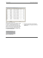
At this point, if all of the runs available were collected it would take 183.98 hours and have a
redundancy of 452.86. Clearly this is not desirable.
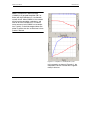
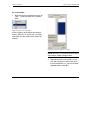
3. Click on Refine Strategy.
4. A list of options will appear. Click on Refine
Strategy again.
Figure 6.16 - Click on Refine Strategy
M86-E00078
APEX2 User Manual
Data Collection
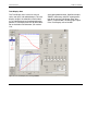
NOTE: The objective in Refine Strategy
(COSMO) is to get good completion (98% or
better) with high redundancy in a reasonable
amount of time. When COSMO is first started it
will tell you the completion, redundancy, and
time for all of the available runs. It is almost
never necessary to let COSMO run to completion. Typically, it should be stopped when completion is greater than 99% and the time is close
to what is desired.
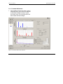
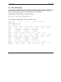
Figure 6.17 - Completeness and Redundancy chart
In this example, as shown in Figure 6.17, the
completion is 99.76% and the time is approximately 2.33 hours.
M86-E00078
6 - 15
Data Collection
APEX2 User Manual
NOTE: Time estimates are approximate. They
depend on the number of rescans, general
instrument overhead, backlash compensation,
etc. If estimated times are consistently longer or
shorter, modify the COSMO hardware profile.
5. Click Stop when the completeness nears
100% and the time and redundancy
approach the desired values. It is not necessary to wait until the refinement reaches
100%.
Figure 6.18 - Strategy Status and Priority control
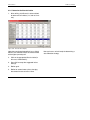
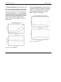
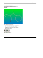
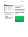
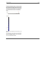
6. Click Refine Strategy.
7. A list of options will appear. Click on Sort
Runs for Completeness.
Figure 6.20 - Completeness and Redundancy charts after
sorting for completeness
Figure 6.19 - Choose “Sort Runs for Completeness”
6 - 16
M86-E00078
APEX2 User Manual
Data Collection
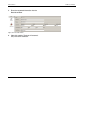
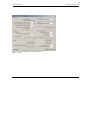
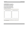
8. To look at the actual runs chosen, go to
View > Detailed Strategy.
This will open a window that shows the runs to
be collected (see Figure 6.21).
Figure 6.21 - Runs to be collected
NOTE: If for some reason it is necessary to start
over, change the distance slightly (by 0.02 for
example) and press Return. COSMO will reload
all of the possible runs.
You are now ready to collect data.
M86-E00078
6 - 17
Data Collection
APEX2 User Manual
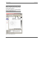
6.4 Data Collection/Run Experiment
1. Click Collect > Experiment.
2. Go back to the experiment window and
delete the three matrix runs if they are still
there.
Figure 6.22 - Deleting the matrix runs
3. Click Append Strategy.
6 - 18
M86-E00078
APEX2 User Manual
Data Collection
4. The program changes the name to the
name of the current project (in this example,
ylid_manual).
Figure 6.23 - Experiment view with strategy appended. In
Version 1.26 and later, the Execute and Resume buttons
are separated. Execute will force the collection of all data.
Resume will start at the point where the data collection was
interrupted.
M86-E00078
6 - 19
Data Collection
NOTE: At the top of the experiment window are
controls for data collection. Usually, the default
values are correct. For data collection times of
less than five seconds, correlation can usually
be turned off. If new dark frames are required,
APEX2 will automatically collect them. Checking
“Generate New Darks” will force the collection of
darks before every run. In Figure 6.23, the time
and width are explicitly set for each run, so
changing the default width and time will have no
effect. If the explicit time or width for a run is
deleted so that the box is empty, the word
“default” appears and the default values at the
top right will be used.
APEX2 User Manual
NOTE: After data collection is started, the
experiment window can be closed and APEX2
can be stopped. The server computer must be
left on. If communications are lost between the
client and the server, frame data is stored on the
server. Typically they will be in the directory
C:\frames\. They should be copied to the correct
project directory before starting integration.
5. Click Execute/Resume. The focus will shift
to Monitor Experiment and images will start
to appear. This may take a minute or two if
new darks are being collected.
NOTE: When resuming after a power failure,
APEX2 will automatically skip images that were
previously collected with matching angles and
generator settings. Otherwise, it will ask if you
want to overwrite the images.
Figure 6.24 - Monitor Experiment view
6 - 20
M86-E00078
7. Data Integration and Scaling
Before the data can be used to solve and refine
the crystal structure, it is necessary to convert
the information recorded on the frames into a
set of integrated intensities, and to scale all of
the data.
M86-E00078
7-1
Data Integration and Scaling
APEX2 User Manual
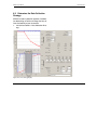
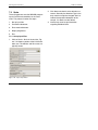
7.1 Integration
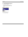
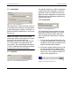
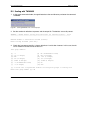
1. Click on Integrate in the task bar.
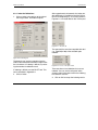
2. Click on the Integrate Images icon. The following window will open.
Figure 7.1 - Initial integration window
3. Check the default values.
There are two items of interest at the top of the
window: the Space Group tool and the Resolution Limit value.
Figure 7.2 - The Space Group tool
7-2
M86-E00078
APEX2 User Manual
The Space Group tool allows the user to set the
symmetry for integration. Typically, this value is
correct when the Integration window opens.
Data Integration and Scaling
At the bottom of the window are two buttons for
defining the data collection runs to be integrated.
Figure 7.5 - The Find and Import Runs buttons
The Import Runs button determines the runs to
be integrated from the experiment that has just
been submitted. Using this button allows the
user to start integration while the data is still
being collected.
Figure 7.3 - Choosing P2(1)2(1)2(1) with the Space Group
tool
The Resolution window on the upper right sets
the upper limit of resolution for integration.
NOTE: SAINT will integrate all of the data currently measured and then will wait for the next
image, integrate that, wait for the next, etc.
The Find Runs button is used to browse to the
set of runs to be integrated. This button is normally used when the data collection is finished.
Figure 7.4 - The Resolution tool
The APEX2 Suite will suggest a resolution cutoff. In this case, the suggested value has been
changed to 0.75.
M86-E00078
7-3
Data Integration and Scaling
APEX2 User Manual
1. Click on Find Runs.
The following window will open. Usually it will
have the correct directory and base name as the
defaults. If these are not correct, then use the
Browse button to find the runs for the data collection of interest.
Figure 7.6 - Find Runs tool view
Both the Import Runs from Experiment and the
Find Runs buttons will generate a list of runs as
shown in Figure 7.7.
Figure 7.7 - Completed runs list
NOTE: To integrate runs from a CD or DVD,
browse to the device and find the runs to be
integrated. APEX2 will automatically write the
result in the work directory for the current
project.
7-4
M86-E00078
APEX2 User Manual
Figure 7.8 shows a run list entry being modified.
(A) shows the original run information. (B)
shows the run with the starting image number
changed to 51. (C) shows the number of frames
to process changed to 111.
Data Integration and Scaling
The default values are generally very good.
There is seldom any need to change those in
the Refine window.
Double-click on any of the fields in this list to
open up that value for editing.
A
B
C
Figure 7.8 - Example of manually editing a run list
2. Check the refinement defaults.
Figure 7.9 - Refine Window
The two buttons on the bottom far left are used
to change the default options for the refinement
of the data.
3. Change the default options for the integration in the “Integration Options” window.
The Integration Options window has a few values that are changed more frequently.
Figure 7.10 - Integration Options window
M86-E00078
7-5
Data Integration and Scaling
APEX2 User Manual
The default values in the Model Profiles window
are usually good.
Figure 7.11 - Model Profiles window
For weakly-diffracting crystals it is sometimes
helpful to change some options in the Model
Profiles window. Reducing the Intensity/Sigma
ratios from 10 and 9 to, for example, 5 and 4 or
3 gives the profile fitting algorithm more reflections to model. Increasing the profile blending by
clicking on “Blend Profiles from All Detector
Regions” can also help with weakly-diffracting
crystals.
4. Click on More Options. This results in an
expanded window (see Figure 7.12) and
gives access to several other useful features, in particular Active Mask (see Figure
7.13), Algorithm (see Figure 7.14), and
Image Queue (see Figure 7.15).
7-6
M86-E00078
APEX2 User Manual
Data Integration and Scaling
Figure 7.12 - The Integration Options window with “More
Options” selected
M86-E00078
7-7
Data Integration and Scaling
7.1.1 Active Mask
APEX2 User Manual
The algorithm buttons are used to change from
narrow to wide frame integration. Frames collected with narrow scan widths (less than one
degree) should be integrated as narrow frames.
Those greater than one degree should be integrated as wide frames.
7.1.3 Image Queue
Figure 7.13 - The Active Mask tool
The Active Mask is used to mask out areas that
are covered by the beamstop, low-temp nozzle,
or other obstructions. Typically a value of 0.7 is
good here. SAINT will determine an active mask
for each run.
NOTE: If this option is set, the user should
examine the active mask images that are written
into the work directory with the name
basename_am_##.sfrm. There is one for each
run. These images can be opened with the
image viewer. They should be blank except for
an area in a different color showing the shape of
the obstruction, typically the beamstop.
7.1.2 Algorithm
Figure 7.15 - The Image Queue tool
The Image Queue sets the number of frames
being used to determine profiles. For crystals
with high mosaic spread (large, wide reflections), increasing the queue size can improve
integration.
5. Click on the Start Integration button on the
far right of the bottom row. This will start the
integration and will open the SaintChart window for monitoring the integration.
6. Examine the output. Double-click on any of
the output entries for one additional tool—
the ls button at the far right of the line (see
Figure 7.16). This will open the SAINT listing file for that integration run.
Figure 7.14 - The Narrow/Wide Algorithm tool
Figure 7.16 - Using the runs list ls tool
7-8
M86-E00078
APEX2 User Manual
Data Integration and Scaling
7.2 SaintChart
SaintChart is a powerful tool for monitoring the
progress of the calculation and for graphically
presenting the results of the integration process.
7.2.1 Monitor the Progress of the Integration
Run
Figure 7.17 - SaintChart view
M86-E00078
7-9
Data Integration and Scaling
As shown in Figure 7.17, when the SaintChart
window opens the graphs are small, and under
Linux the text area is large.
APEX2 User Manual
Expand the windows to fill the available image
area by clicking on the four-square icon
in
the upper left (see Figure 7.18).
If desired, change the view.
Change the text area by clicking and dragging
on the line between the text and image areas.
Figure 7.18 - SaintChart view with graphical area expanded
7 - 10
M86-E00078
APEX2 User Manual
Data Integration and Scaling
To the right of the image area are a series of
check boxes that select the displays.
1. Click on the check boxes to add or remove
displays. Click on Integration Progress to
add the new display seen in Figure 7.19.
When the integration is complete, the blue
progress bars will be full and the remaining
time will be zero.
Figure 7.19 - Integration Progress display
M86-E00078
7 - 11
Data Integration and Scaling
APEX2 User Manual
2. Click on Spot Position Overlay (in PerImage Statistics) to add one of the most
powerful windows for monitoring the
progress of the integration. Pull up on the
Window Tool Bar for Integrated Spots (the
cursor arrow is pointing to this tool bar in
Figure 7.20) to display the entire window
(see Figure 7.21).
Figure 7.20 - Spot Position Overlay
7 - 12
M86-E00078
APEX2 User Manual
Data Integration and Scaling
In this full view, the Integrated Spots window
looks much like the image viewer used previously. At the bottom of the window is an entry
box that can be used to change the display frequency of the Integrated Spots images. The
default is to display every fifth image.
Figure 7.21 - Full view of the Spot Position Overlay
M86-E00078
7 - 13
Data Integration and Scaling
APEX2 User Manual
7.2.2 Examine Final Results
At the end of integration, examine this text critically. In particular, look at the Overall Rsym, the
Coverage Statistics and the Unconstrained Unit
Cell refinement.
1. Set up to view SAINT text output. At the bottom of the SaintChart window is a scrolling
text window that displays the text output
from SAINT. (This window can be expanded
by dragging the horizontal bar above the
text as indicated by the position of the
mouse cursor in Figure 7.22).
2. Examine the final results.
2.1 Overall Rsym and Coverage Statistics
(Figure 7.22)
The overall Rsym is usually less than 8%.
Higher values may indicate problems with
absorption, twinning or poor crystal quality.
Overall
Coverage
Figure 7.22 - Final SAINT Overall Rsym and Coverage
Statistics
7 - 14
M86-E00078
APEX2 User Manual
The coverage statistics are reported by resolution shells. The values in the Rsym column give
the cumulative agreement of equivalent reflections. The Rshell values give agreement within a
particular shell. These change faster than the
Rsym values. The %<2s column is useful for
checking where the weak data becomes predominant (greater than 50 or 60%). The #Sigma
column gives the average I/sigma for each shell.
If that number is less than 1.5 or 2, then little significant data is being measured in that shell.
Data Integration and Scaling
2.2 Unconstrained Unit Cell Refinement
(Figure 7.23)
Check the angles in the unconstrained unit cell
refinement to get a quick confirmation that the
initial lattice determination was correct. In the
unconstrained refinement, angles that are
required to be 90 or 120 are allowed to refine. If
they differ considerably from the expected
value, then the data should be checked carefully.
Figure 7.23 - Unconstrained unit cell refinement
M86-E00078
7 - 15
Data Integration and Scaling
7.3 Scale
The scaling process uses the SADABS program
to put all of the measured data on the same
scale. This process involves five steps:
1. Set up input files.
2. Parameter refinement.
APEX2 User Manual
2. Click Next and check that the defaults are
correct. Generally the Absorber Type is the
only value that might be changed. Set it to
indicate the expected absorption of the
sample. If in doubt, use the default.
3. Use the help arrow to get information
regarding individual items.
3. Error model refinement.
4. Display diagnostics.
5. Exit.
7.3.1 Set up Input Files
1. Click on Scale > Scale in the task bar. Figure 7.24 shows a portion of the initial Scale
work area. The defaults and file names are
typically correct.
Figure 7.24 - Input setup window
7 - 16
M86-E00078
APEX2 User Manual
Data Integration and Scaling
7.3.2 Parameter Refinement
1. Click on Refine. Figure 7.25 shows a typical
refinement result. The R-values are reduced
and the Mean Weight increases. Typical
final values are 3–4% for the R-values and
0.95–0.98 for the Mean Weight.
Figure 7.25 - XScale window after refinement
M86-E00078
7 - 17
Data Integration and Scaling
APEX2 User Manual
7.3.3 Error Model Refinement
Figure 7.26 shows typical Error Model results.
Figure 7.26 - Error Model results
If the R-values in one run are significantly higher
than the others, you can repeat the entire scaling calculation with that run omitted. Click the
check box by the “bad” run and then click
Repeat Parameter Refinement.
7 - 18
M86-E00078
APEX2 User Manual
7.3.4 Examine Display Diagnostics
The Display Diagnostics provide valuable
insight into the quality of the data and possible
problems with the data. Click on the tabs at the
bottom of the screen to view diagnostic data.
1. Click Finish to produce a series of diagnostic plots. Some of these are reviews of the
plots that have already been displayed.
Data Integration and Scaling
The Scale Variations plot (Figure 7.27) shows
the overall variation in Scale and R(int) for the
individual frames. The Scale plot should be flat
(for highly absorbing, irregularly shaped crystals
it will probably be sinusoidal) and the R(int) plot
should not show large variations (more than
2%).
Figure 7.27 - Overall Scale and R(int) variations
M86-E00078
7 - 19
Data Integration and Scaling
The Intensity Statistics plots look at R(int) and
|E2-1| as a function of resolution. Typical plots of
R(int) versus resolution increase to the right as
seen in Figure 7.28. An |E2-1| plot should have
a constant resolution. |E2-1| is a strong indicator
of centric and acentric space groups. The two
horizontal lines indicate the expected values for
centric (top) and acentric (bottom) space
groups. This plot clearly suggests an acentric
space group.
APEX2 User Manual
The plots of Chi-Squared values for the data as
a function of resolution and intensity should be
mostly flat. Values below one are not unusual
for weaker high-resolution data. The plots
shown in Figure 7.29 are typical.
Figure 7.29 - Chi-squared
Figure 7.28 - Intensity Statistics
7 - 20
M86-E00078
APEX2 User Manual
Data Integration and Scaling
The Spatial Distribution plots are generated
for each data collection run. They indicate, using
red and blue dots, points of average intensity for
a particular reflection after scaling. The actual
intensity measured at that spot on the detector
may vary by more than three standard deviations. Figure 7.30 shows two spatial distribution
plots side by side. This is the way they are typically output by the scaling process.
Figure 7.30 - Spatial distribution
M86-E00078
7 - 21
Data Integration and Scaling
Figure 7.31 shows a single plot so that the dots
are easier to see. Note that the points of disagreement are spread fairly evenly over the
entire detector face.
APEX2 User Manual
If the spots are clustered in an area or if there
are significantly more spots of one color than
there are of another, then the data should be
examined critically. Figure 7.32 is from another
data set where the Active Mask was not used
during integration and the reflections collected
in that area are consistently smaller than
expected. This kind of problem may affect the
final results.
Figure 7.31 - A single Spatial Distribution
Figure 7.32 - A Spatial Distribution plot showing a problem
area
7 - 22
M86-E00078
APEX2 User Manual
Data Integration and Scaling
7.3.5 Exit
1. Click on Exit AXScale to close the scaling
GUI.
Figure 7.33 - Exit AXScale
NOTE: Scale is one of the few GUIs where it is
necessary to exit using a special Exit button.
This avoids an error message indicating that
SADABS has exited improperly.
M86-E00078
7 - 23
Data Integration and Scaling
7 - 24
APEX2 User Manual
M86-E00078
8. Examine Data
In this step, the space group for the sample is
determined and optional simulated precession
photographs are calculated to further evaluate
the overall quality of the data. APEX2 provides
two tools for this: XPREP for space group determination and Precession Images for looking at
undistorted slices of reciprocal space. This is
the final step before beginning the structure
solution and refinement process.
8.1 XPREP
1. Click on XPREP (Space Group Determination) under Examine in the task bar.
2. Check that the two files in the pop-up window are correct (see Figure 8.1) and click
OK.
M86-E00078
Figure 8.1 - Select files for XPREP input
NOTE: In this example, the scaling process has
created two files: ylid_manual_0m.p4p containing the final unit cell parameters from integration
and ylid_manual_0m.hkl containing the corrected intensities. Typically, these are the files
to use for determining space groups, but you
can browse to choose other files.
8-1
Examine Data
APEX2 User Manual
8.2 Space Group Determination
1. XPREP evaluates the data and looks at the
mean intensities and the mean int/sigma.
Since these are large for all groups except
P, XPREP suggests that the lattice is P (see
Figure 8.2). Press Enter to accept.
Figure 8.3 - Reduced cell
For the YLID, no higher symmetry cell is found.
The program has determined that the YLID crystal has an orthorhombic primitive lattice (see
Figure 8.4). Press Enter to accept.
Figure 8.2 - Lattice statistics
2. XPREP determines the reduced cell based
on the lattice entered above. Since the lattice was primitive and the magnitudes of the
cell dimensions were proper (a<b<c), the
original and reduced cells are the same
(see Figure 8.3). Press Enter to search for a
higher symmetry cell.
8-2
Figure 8.4 - Higher symmetry cells
M86-E00078
APEX2 User Manual
3. The next logical step is to determine the
space group. XPREP suggests this (see
Figure 8.5). Press Enter to determine the
space group.
Examine Data
5. XPREP has chosen the crystal system [O]
(see Figure 8.7). Press Enter to accept.
Figure 8.7 - Choose the crystal system
6. XPREP has chosen the crystal lattice [P]
(see Figure 8.8). Press Enter to accept.
Figure 8.5 - Determine the space group
4. If the space group is known or if the compound is known to be chiral, enter that information (see Figure 8.6). Generally, it is
sufficient to press Enter to start the space
group determination.
Figure 8.6 - Space Group options
M86-E00078
Figure 8.8 - Choose the lattice
7. XPREP evaluates the data and looks at the
systematic absences for all possible glide
planes and screw axes (see Figure 8.9).
These are displayed across the middle of
the figure. By examining the number of
reflections with I>3 sigma(I), the mean
intensities, and the mean int/sigma, which
should all be very small for a systematic
absence, XPREP derives a suggested
space group, P2(1)2(1)2(1). Press Enter to
accept.
8-3
Examine Data
8.3 Reflection Statistics.
APEX2 User Manual
3. The data can be merged in several ways.
Choose the “Merge ALL equivalents including Friedel opposites” option [A] (see Figure
8.11). Press Enter to accept.
NOTE: This merge will not average the reflections in the final data file. It is only for the calculation of statistics.
Figure 8.9 - Systematic absences and a suggested space
group
1. XPREP returns to the general menu seen
previously (see Figure 8.5). This time D is
chosen to evaluate the data set. Press
Enter to accept.
2. There are multiple choices for data manipulation (see Figure 8.10). “S” chooses a display of statistics.
Figure 8.10 - The data manipulation menu
8-4
Figure 8.11 - The merge data menu
4.
A table of statistics appears (see Figure
8.12). Examine the data presented. Is the
completion near 100%? Is the redundancy
good? Are Rint and Rsigma small and
increasing smoothly from top to bottom? In
particular, look at the last two lines which
compare all of the data with the high-resolution data. The completion should be near
100% for both the high-resolution shell and
the complete data set. The redundancy and
Rint should be similar for the two. The Mean
Intensity and the Mean I/sigma(I) will usually
be quite different. The Mean I/sigma(I) for
the high-resolution data should be greater
than 3.0.
M86-E00078
APEX2 User Manual
For this data set, when integrated to 0.67Å resolution, the difference between the Rint for the
high-resolution data and the complete data set
is slightly larger than expected. Press Enter to
continue.
Examine Data
1. Since the difference between the Rint for
the high-resolution data and the complete
data set is slightly larger than expected, it is
reasonable to apply a high-resolution cutoff
using the H option in the data manipulation
menu. (see Figure 8.13). Type H and press
Enter.
Figure 8.13 - Requesting a high resolution cutoff
Figure 8.12 - Intensity statistics
2. Enter a high resolution limit of 0.75 (see Figure 8.14) and press Enter to accept the low
resolution cutoff of infinity.
8.4 Applying High Resolution Cutoff
NOTE: For the YLID crystal, if the resolution
limit for integration was changed to 0.75 as suggested on Page 7-3, then there will be no need
to apply a High Resolution Cutoff at this point.
M86-E00078
Figure 8.14 - The resolution cutoff menu
8-5
Examine Data
3. Applying the cutoff removes approximately
3000 reflections from the data set (see Figure 8.15). The next step is to see if the cutoff has improved the statistics. Type S and
press Enter.
APEX2 User Manual
5. After the cutoff, all of the statistics look better (see Figure 8.16). Press Enter to continue.
Figure 8.16 - Statistics after high resolution cutoff
Figure 8.15 - Requesting statistics after applying a high
resolution cutoff
4. As in step 3 of Section 8.3, enter [A] to
merge all equivalents.
8-6
6. This response will return to the data manipulation menu (see Figure 8.10, Figure 8.13
or Figure 8.15). The default answer should
be E for Exit. Press Enter to accept this
default and return to the general menu.
M86-E00078
APEX2 User Manual
Examine Data
8.5 Preparing an Output File
1. In the general menu, chose C to define the
unit cell contents.
2. A window will open displaying the current
formula, Z, the density, and the atomic volume (see Figure 8.17). In this example, the
formula is incorrect and Z has been set to
six to try to achieve a reasonable density
and atomic volume. Since this formula is
incorrect, it must be modified now. The correct chemical formula for the YLID crystal is
C11H10O2S.
2.1 At Select Option, do not accept the
default answer of E. Type in F to enter a
new formula.
2.2 In response to the question “Enter Formula,” type the correct formula C11
H10 O2 S1 and press Enter.
2.3 Check that the information is correct.
Check that Z seems reasonable for the
space group, that the density is as
expected (1.1 to 1.4 for organic molecules, higher for inorganic compounds),
and that the atomic volume is around
17 or 18. Significant variation from the
expected values may indicate an incorrect molecular formula or missing
counter ions or solvates. The values at
the bottom of the window look fine for
the YLID. Press Enter to accept.
M86-E00078
Figure 8.17 - Defining and checking the unit cell contents
3. The next default action for XPREP is to
write out the files necessary for the structure
solution process (see Figure 8.18). Press
Enter to accept.
Figure 8.18 - Requesting output files
8-7
Examine Data
APEX2 User Manual
4. The program asks for an output file name.
Since this data has been cut off at a resolution of 0.75A, it makes sense to change the
output file name to ylid_res75 to reflect the
cutoff (see Figure 8.19). Press Enter to
accept.
Figure 8.20 - The input file for structure solution and a final
question
6. Exit XPREP (see Figure 8.21). Press Enter
to exit the program.
Figure 8.19 - Changing the file name
5. After entering the file name (or hitting Enter
to accept the default file name) an input file
for the structure solution module is created
and displayed on the screen, and the program asks, “Do you wish to (over)write the
intensity data file ylid_res75.hkl?” Since the
file name has been changed, this question
must be answered with a y (see Figure
8.20).
8-8
Figure 8.21 - Exit XPREP from the general menu
NOTE: There are many other features in
XPREP that can be accessed from the general
menu; reciprocal space plots, simulated powder
patterns and a test for merohedral twinning are
very useful tools.
M86-E00078
APEX2 User Manual
8.6 Simulated Precession Images
1. Click on Precession Images under Examine
in the task bar. Precession Images provide
an undistorted view of layers of the reciprocal lattice. APEX2 generates simulated precession images by finding the appropriate
pixels in a series of “.sfrm” images. You
must specify the images to examine and the
zones to calculate.
2. To open the File Selection window, left-click
on the folder beside the file name. Choose
the sets of images that you want to use for
the calculation by clicking on the check
boxes (see Figure 8.22).
Examine Data
3. Check the default input value. Modify as
needed and press Calculate.
Calculating more zones does not significantly
increase the calculation time. In the example,
1kl, h1l and hk1 have been added to the
defaults of 0kl, h0l and hk0. Fractional values
(e.g., 0.5kl) are allowed. Reducing the resolution may speed the calculations slightly. The
thickness defines the range of pixels above and
below the requested range. For example, if the
0kl zone is requested with a thickness of 0.1,
then the simulation is looking for all pixels that
have -0.1<h<0.1, and any value (including fractional values) for k and l.
Figure 8.23 - Detail of the input section
Figure 8.22 - File Selection window with matrix runs
deselected
M86-E00078
8-9
Examine Data
4. A progress bar will appear (Figure 8.24) and
after approximately 5–10 minutes (depending on the number of “.sfrm” files read) an
image will appear on the screen. Display
other planes by clicking on the calculated
images to the bottom right of the work area
or by browsing as usual with the View plugin.
APEX2 User Manual
5. Use the simulated patterns to check space
group symmetry (see Figure 8.25, Figure
8.26 and Figure 8.27) and to find signs of
twinning (see Figure 8.28).
Figure 8.24 - Progress bar
Figure 8.25 - The 0kl plane for the test YLID
8 - 10
M86-E00078
APEX2 User Manual
Figure 8.26 - The h0l plane for the test YLID
M86-E00078
Examine Data
Figure 8.27 - The hk0 plane for the test YLID
8 - 11
Examine Data
APEX2 User Manual
Figure 8.28 - A plane from a rotationally twinned crystal
showing the two lattices
8 - 12
M86-E00078
9. Structure Solution and Refinement
9.1 Overview
You are now ready to solve and refine the crystal structure. The various steps in solving and
refining the structure are carried out within the
APEX2 GUI. XPREP has prepared the input
files for a standard direct methods run. There
are two files: .ins and .hkl. In this example, the
two files are ylid_res75.ins and ylid_75.hkl.
M86-E00078
These files are all that is required to begin the
structure solution and refinement process. The
various steps of solving and refining the structure are carried out using the Solve and Refine
functions of the APEX2 Suite.
9-1
Structure Solution and Refinement
9.2 Solve the Structure
The process of obtaining an initial model of the
compound is started by clicking in the Task Bar
on Solve Structure and then on Structure Solution.
1. This will open the Structure Solution GUI.
Check that there is a reasonable formula in
the formula window.
APEX2 User Manual
1.1 If you entered a correct formula in the
display GUI, then you are ready to start
a normal direct methods run.
1.2 If the formula is incorrect, change it in
the formula window and press Return.
The input file will update.
Figure 9.1 - Default Solve Structure view
9-2
M86-E00078
APEX2 User Manual
2. Click on Solve Structure to start the calculations and open an output window. This window can be used to monitor the progress of
the direct methods calculations.
Structure Solution and Refinement
In most cases the default values will give a good
initial model, but there are several other options
available for more difficult problems.
1. Chose the solution method by clicking the
appropriate radio button on the left in the
Method box.
2. Highlight and click on Direct 1 to set up a
default run with a simple TREF instruction.
3. Highlight and click on Direct 2 to set up an
extended run with TREF 10000. By adding
10000 to the TREF command, more
attempts are made to determine a solution.
This will take more time, but if you see a
good solution in the output window it is possible to stop at that point by clicking on the
STOP button. Good solutions typically have
a CFOM of 0.06 or less.
Figure 9.2 - Structure Solution output
3. Click on the arrow to the right of Direct 1 in
the Method box (see Figure 9.3). This gives
three choices for structure solution using
direct methods.
4. Highlight and click on Direct 3 to set up an
extreme run with two instructions, ESEL 1.0
and TREF 100000. By adding ESEL 1.0,
more reflections are used in the solution
process. Increasing the number of tries in
the TREF command to 100000 runs (until
ended by clicking on the STOP button) is
particularly useful for acentric triclinic structures and for pseudo-symmetric structures.
There is only one pre-defined option for the
dual space calculations and also only one
for the heavy atom Patterson methods.
Figure 9.3 - Method box
M86-E00078
9-3
Structure Solution and Refinement
At the end of the direct methods runs, the output
display will look like Figure 9.2. Good figures of
merit are near 1.0 for Sigma-1 and M(abs) and
less than 0.06 for Ralpha and the CFOM. Structures can be solved with figures of merit that
deviate from these numbers, but they may
require more effort.
If the initial model looks reasonable, click OK in
the output display and Exit in the Solutions plugin. The next step is structure refinement using
XShell.
APEX2 User Manual
9.3 XShell
9.3.1 Refine the Structure
The structure solution step produced statistics
indicating that a solution had been found. The
real proof, however, is in the initial model that is
produced. XShell provides the tools to view and
refine the model. A quick glance at the results of
the direct methods run is often all that is needed
to see that the results make chemical sense.
Control of the refinement process is quite
straightforward using XShell.
1. Start XShell, the molecular viewing and
refinement plug-in, by clicking on Refine
Structure in the Task Bar and then on the
Structure Refinement icon.
2. This will open a window to select files for
XShell. In usual operations, the file name
will be pre-selected. If a different file is
desired, select Browse.
Figure 9.4 - The Select Files tool
9-4
M86-E00078
APEX2 User Manual
Structure Solution and Refinement
3. Click on OK to open a molecular display
window.
Figure 9.5 - Initial view of the YLID molecule
M86-E00078
9-5
Structure Solution and Refinement
APEX2 User Manual
4. Right-click in the background to open a popup window with options to change the
image.
Figure 9.6 - XShell menu
5. Click on the Information On All Atoms option
to open a window displaying a list of the
peaks and their heights (see Figure 9.7).
The drop in height between Q13 (the last
real peak) and Q14 (the first noise peak) is
typical of a correct solution. Click on OK to
close this window.
9-6
M86-E00078
APEX2 User Manual
Structure Solution and Refinement
Figure 9.7 - Atom information screen
At the bottom right of the main window is a slide
bar which is used for deselecting peaks. The
arrow can be moved by left-clicking and dragging the arrow or by left-clicking on either side of
the arrow. Left-clicking to the left of the arrow
(i.e., where the mouse cursor is pointed in Figure 9.8) will remove peaks.
6. Slide the pointer down while watching the
molecular display. Change the number of Q
peaks to 15.
Figure 9.8 - The Q peak slider
M86-E00078
9-7
Structure Solution and Refinement
APEX2 User Manual
At 15 the molecule is much cleaner, but there
are still peaks that do not make sense.
Click left on the slider until you find a reasonable
model.
Figure 9.9 - Image after the number of Q peaks was
changed to 15
Figure 9.10 - Image with all noise peaks removed
9-8
7. Put the cursor over the bonds to check distance. The distance will be displayed at the
bottom right.
M86-E00078
APEX2 User Manual
Structure Solution and Refinement
9.3.2 Label the Atoms
1. Label the atoms and set the atom types.
Left-click on atoms to select them. Left-click
on the peaks for the two oxygen atoms (Q2
and Q5 in this example).
Figure 9.11 - View of model with the probable oxygen peaks
selected
M86-E00078
9-9
Structure Solution and Refinement
APEX2 User Manual
2. If it is difficult to see the color and labels,
change the color scheme by left-clicking on
Preferences and then right-clicking on
Background Color. Choose colors and click
Apply. Click Cancel to exit the background
color mode. Note that the selected peaks
are blue in Figure 9.13.
Figure 9.12 - Selecting the background color
9 - 10
M86-E00078
APEX2 User Manual
Structure Solution and Refinement
The Atom Labelling box will open.
Figure 9.15 - Atom Labelling box
4. The two selected atoms need to be
changed to oxygen atoms. Do this one of
two ways:
Figure 9.13 - New background color
•
3. Right-click to view a pop-up menu and
select Labelling.
Click on the Element field and type in the
element symbol (case does not matter).
•
Click on the El button to the right of the Element field. This will open a periodic table.
Left-click on the appropriate element symbol to select it (the periodic table will automatically close).
Figure 9.14 - Select Labelling
M86-E00078
9 - 11
Structure Solution and Refinement
APEX2 User Manual
Figure 9.16 - The periodic table for selecting atom types
5. Once the element type is set correctly, click
on Relabel to number the peaks sequentially in the order they were selected, starting with the number in the First Sequence #
field.
9 - 12
M86-E00078
APEX2 User Manual
6. Seeing the color of atoms can be difficult in
the Wireframe view used so far. Right-click
in the background with no atoms selected to
get a slightly different action menu. In this
menu, highlight and left-click on Pipes. This
makes the bonds thicker and makes it obvious that there is an incorrectly labeled atom.
This will be corrected when the carbon
atoms are labeled.
Structure Solution and Refinement
7. Left-click on the remaining peaks in the
order that you want them labeled.
NOTE: If working on YLID test data, look at Figure 9.18 and click on the peaks to give the same
order as used here. Right-click and choose
Labelling. Select Carbon and apply the labels.
8. In the Labelling tool, change the element
type to C (carbon). The starting atom number will change to 1—the first available
number for carbon atoms.
9. Click Relabel.
10. Click Cancel to close the window.
Figure 9.17 - Choose the pipes view
M86-E00078
9 - 13
Structure Solution and Refinement
APEX2 User Manual
9.3.3 Refine the Molecule
The labeled YLID molecule is now ready for
refinement.
Figure 9.18 - Correctly labeled model
1. Left-click on the Refine icon in the tool icon
bar (the cursor is pointing to it in Figure
9.19) or Type Control+R or go to Refine in
the Windows tool bar.
Figure 9.19 - The Refine icon
9 - 14
M86-E00078
APEX2 User Manual
This will open the Refine Box. Click on Refine to
launch XL (the least-squares refinement program) using the default parameters as given.
Structure Solution and Refinement
After a few seconds, a Refine window will open
with output results for the calculation.
Figure 9.21 - Isotropic refinement output
Figure 9.20 - The Refine menu
In the output displayed above, note that the R1
value is 0.08. This is typical for a preliminary isotropic refinement for an organic molecule with
data to a resolution of 0.75 and no hydrogen
atoms included. The refinement program also
indicates that the model needs to be inverted to
get the correct absolute structure.
NOTE: This indication of the absolute configuration is usually reliable, but all assignments of
absolute structure should be confirmed later in
the refinement process by including TWIN and
BASF cards in the instruction input.
M86-E00078
9 - 15
Structure Solution and Refinement
APEX2 User Manual
2. Click on OK to return to XShell. The molecule display will refresh with the results of
the least-squares calculations.
Figure 9.22 - The model after isotropic refinement
The peaks in the diagram represent difference
in the electron density between the refinement
model and the experimental electron density as
defined by the measured data. Many of these
difference peaks are near the sulfur and oxygen
atoms. Refinement of all atoms anisotropically
should improve the model.
3. In the refinement box, click on Invert Structure and Refine All Non-H Atoms Anisotropically as in Figure 9.23.
Figure 9.23 - Inverting and choosing anisotropic refinement
9 - 16
M86-E00078
APEX2 User Manual
Structure Solution and Refinement
4. Click on the Refine button to launch the
least-squares refinement program. The output window will open and a summary of the
results of individual cycles of refinement will
appear.
Figure 9.24 - Least-squares refinement summary
The value for R1, 0.047, is typical for an initial
anisotropic refinement with no hydrogen atoms
included. Since the mean shift/esd is greater
than 0.1, the model is still changing. Since the
highest peak in the difference map has a height
of 0.49 and is 0.5Å from C10, there are certainly
some hydrogen atoms to be included.
M86-E00078
9 - 17
Structure Solution and Refinement
APEX2 User Manual
Examination of the difference peaks in the
resulting difference electron density map shows
that the top difference peaks all correspond to
hydrogen atoms.
Figure 9.25 - Difference peaks correspond to expected
hydrogen atom positions
9 - 18
M86-E00078
APEX2 User Manual
Structure Solution and Refinement
9.3.4 Look at Atomic Displacement
Parameters (Thermal Ellipsoids)
It is generally good practice to examine the displacement parameters at this point in structure
determination.
1. Remove difference peaks with the slider
tool.
Figure 9.26 - Removing all Q peaks with the slider bar
2. Right-click on the background and select
Thermal Ellipsoids.
Figure 9.28 - Thermal Ellipsoid plot
Figure 9.27 - Selecting Thermal Ellipsoids
3. Right-click on the background and click on
Information on All Atoms.
Alternatively, a list of Ueq’s (equivalent isotropic
displacement parameters) can be generated by
requesting information on all of the atoms.
Examining these values for outliers is good
practice.
Figure 9.29 - Selecting Information on All Atoms
M86-E00078
9 - 19
Structure Solution and Refinement
APEX2 User Manual
This produces the table in Figure 9.30.
Figure 9.30 - List of parameters with Ueq to the right
Examining the values here is difficult because
the atoms are not in order.
9 - 20
M86-E00078
APEX2 User Manual
Structure Solution and Refinement
9.3.5 Sort Atoms
1. Right-click on the background and click on
“Sort…” to sort the atoms into a sensible
order.
Figure 9.31 - Choose the Sort option
A box will appear to the right of the molecule
display. Since S1, O1 and O2 are in a reasonable order, only the carbon atoms need to be
ordered.
Figure 9.32 - Selecting carbons for sorting
NOTE: Generally, it is easier to sort and number
atoms before adding hydrogen atoms.
2. Highlight the atoms to be sorted (i.e., leftclick and drag over the atoms) and move
them to the Sort Bin (i.e., left-click on Move
Selected Atoms to Sort Bin).
M86-E00078
9 - 21
Structure Solution and Refinement
APEX2 User Manual
4. Highlight O2 and click on Insert All After as
in Figure 9.34.
Figure 9.33 - Carbon atoms in Sort Bin
3. After the atoms are in the Sort Bin, click on
Sort(Alpha-Numeric) to get them into a normal order.
Figure 9.34 - Sorted atoms with “insert after” atom (O2)
selected.
5. Click on OK to accept the sorting.
Figure 9.35 - OK button
9 - 22
M86-E00078
APEX2 User Manual
The resulting list of atom information is easier to
examine.
Structure Solution and Refinement
9.3.6 Add Hydrogen Atoms
At this point, refine the hydrogen atoms either
by renaming the Q peaks using the Labelling
tool as before and then including them in the
refinement, or include the hydrogen atoms in
fixed idealized positions riding on the atom to
which they are attached.
In this manual we will illustrate the latter fixed
idealized method.
Figure 9.36 - Sorted atoms
The Ueq are reasonable if there are:
•
lower values for the sulfur atom and the fivemember ring
•
higher values for the terminal atoms—methyls and carbonyls
•
sensible numbers for the six-member ring—
lower for C8 and C9, higher for C5 and C6,
and in between for C4 and C7.
NOTE: In some cases (e.g., hydrogen atoms on
hetero atoms or on geometrically strained carbon atoms), it is better to refine the hydrogen
atom positions. A general rule is to refine if there
is some doubt about the position of the hydrogen atom and there is difference electron density present.
1. Using the slider tool, remove all of the Q
peaks.
Figure 9.37 - Refined model with difference peaks removed
M86-E00078
9 - 23
Structure Solution and Refinement
2. Right-click in the background and click on
Hybridize All.
APEX2 User Manual
3. The following warning will appear indicating
that the hydrogen atoms have been provisionally added and that the final addition
with naming will take place when the leastsquares calculations are started. Click OK.
Figure 9.38 - Hybridize button
The colors of the atom labels will change to indicate the atom hybridization.
NOTE: If the atom hybridizations are hard to
see, right-click on the background and open the
Information on All Atoms window.
Figure 9.41 - Hydrogen atom warning
Figure 9.39 - Calculate Hydrogens button
Figure 9.40 - Model with added Hydrogen atoms
9 - 24
M86-E00078
APEX2 User Manual
Structure Solution and Refinement
4. Click on the Refine button to launch the
least-squares refinement program. The output window will open and a summary of the
results of individual cycles of refinement will
appear.
Figure 9.43 - Difference peaks in a well-refined model
9.3.7 Final Refinement for Publication
Obtain a view that is much easier to interpret by
reducing the number of difference peaks in the
Refine menu (see Figure 9.44).
Figure 9.42 - Refinement results
The value for R1, 0.029, is typical for an anisotropic refinement with riding hydrogen atoms
and a data set measured to 0.75Å. Since the
mean shift/esd is less than 0.01, the model is
not changing significantly. Since the highest
peak and the deepest hole in the difference map
are similar, there are probably no missing
atoms.
The resulting difference electron density map
appears rather ugly. This is because the number
of difference peaks to be displayed has been left
at 20.
M86-E00078
1. For the final cycles of refinement, reduce
the number of peaks to be displayed to five
and turn on “Use Suggested Weights” and
“Generate ACTA(CIF) Information File” as
shown in the next two figures.
NOTE: If the suggested weights vary significantly from 0.06 and 0.00, then change the values to 0.06 and 0.00.
Figure 9.44 - Reduce the number of difference peaks
9 - 25
Structure Solution and Refinement
APEX2 User Manual
Figure 9.47 - Open the .ins file for editing
3. Check that the temperature card is correct.
Figure 9.45 - Select weights and request ACTA output
Figure 9.46 shows a difference map with the
number of peaks set at five.
4. If torsion angles are of interest, add a CONF
(confirmation) card (see Figure 9.48).
Figure 9.48 - Add instructions in the .ins file
5. If planarity and angles between planes are
of interest, add mpla cards.
Figure 9.46 - Difference peaks
2. Click on Edit File, choose INS and click OK
to open the instruction file for XL. This
allows you to add instructions that are not
directly available in the GUI.
9 - 26
M86-E00078
APEX2 User Manual
9.3.8 Generate an Atomic Displacement
(Thermal Ellipsoid) Plot
1. Remove difference peaks with the slider
tool.
Structure Solution and Refinement
At the top of the box that is opened, there are
three values that can be changed to adjust the
size of atoms and the bonds to them.
2. Right-click on the background and select
Thermal Ellipsoids.
Figure 9.51 - Default atom preferences
4. Change the hydrogen radius to 0.08 and the
bond radius to 0.15 to make the hydrogen
atoms smaller.
Figure 9.52 - Modified atom preferences
Figure 9.49 - Thermal ellipsoids with large hydrogen atoms
3. If the hydrogen atoms in Figure 9.49 are
large, change their size.
3.1 Click on Preferences in the Window
Tool Bar and choose Atom Preferences.
Figure 9.50 - Atom Preferences tool
M86-E00078
Figure 9.53 - Thermal ellipsoid plot with smaller hydrogen
atoms
9 - 27
Structure Solution and Refinement
APEX2 User Manual
5. Position atom labels by right-clicking on the
atom and choosing Position Label.
Figure 9.56 - Generate JPEG
Figure 9.54 - Position Label menu
NOTE: A message may appear that the font file
needs to be defined: “Please set your font directory for the first time for opengl rendering.” If this
happens, click on Preferences > OpenGL Preferences. Then click on the TrueType font
For.OpenGL. In Windows, browse to
C:\bn\xshell\fonts\ or in Linux go to /usr/local/
bin/xshell/fonts. Choose a font.
Figure 9.55 - Positioned labels
6. Convert this image into a high-quality .jpg
file for inclusion into reports by clicking on
render in the Windows Tool Bar and choosing Black and White to High Quality JPEG
file.
9 - 28
M86-E00078
APEX2 User Manual
Structure Solution and Refinement
Figure 9.57 - The final rendered thermal ellipsoid/atomic
displacement parameter plot
M86-E00078
9 - 29
Structure Solution and Refinement
9 - 30
APEX2 User Manual
M86-E00078
Appendix A. RLATT
RLATT is a very powerful tool for viewing the
harvested reflections in a reciprocal lattice. This
section will cover only a few of its features.
RLATT is best learned through use.
A.1 Open RLATT
This example has over 3300 reflections. This is
not the typical case; generally only 300 or 400
reflections are examined. Using extra reflections
will make the examples easier to see.
2. Click on the Start icon to read the reflections
from the database into RLATT.
1. Start RLATT from the Task Menu under
“Examine Crystal.”
Figure A.1 - RLATT icon
M86-E00078
A-1
RLATT
APEX2 User Manual
Figure A.2 is a typical unoriented view after
import. The gray circles are more intense reflections, i.e., those with higher I/sigma(I). The black
dots represent less intense reflections. The
intensity key slider at the bottom of the window
can be used to change the selection criterion.
Figure A.4 - Full menu tools
Additional context-sensitive information is available by left-clicking on the “What’s This” help
arrow in the menu bar.
Figure A.5 - The “What’s This“ help arrow
Figure A.2 - Unoriented RLATT view
Other tools can be accessed by right-clicking on
the background to give the “Quick Tools” menu
(Figure A.3) and by clicking on RLATT in the
menu bar (Figure A.4).
For example, clicking on the help arrow and
then clicking in the work area (the gray area to
the right of the lattice display) gives the display
of shortcuts shown in Figure A.6. Clicking on the
blue background gives the hints shown in Figure
A.7.
Figure A.3 - Quick Tools menu
A-2
M86-E00078
APEX2 User Manual
RLATT
Figure A.6 - Shortcut keys and commands
M86-E00078
A-3
RLATT
APEX2 User Manual
Figure A.7 - Help for the 3D display obtained by clicking the
“What’s This” arrow on the blue display background
A-4
M86-E00078
APEX2 User Manual
A.2 Orienting Views
Move the mouse to rotate the RLATT display. It
is possible to easily see rows and non-fitting
peaks (see Figure A.8).
Figure A.8 - RLATT display looking down layers of
reflections
M86-E00078
RLATT
By sliding the intensity key at the bottom of the
display, it is easy to deselect weak reflections.
In Figure A.9 the reflections between the layer
lines all go black when the intensity filter is
moved to the left.
Figure A.9 - RLATT display looking down layers of
reflections. Weaker reflections, i.e., those with smaller I/
sigma(I), are black because the “Intensity Filter” slider
(bottom left) has been moved slightly to the left.
A-5
RLATT
With additional rotations, the layers of reflections can be further oriented so that stacks of
reflections become visible. Sometimes it is quite
useful to right click on the background and
choose Z-rotations from the rotation options.
The 2D profiles on the top and to the left are a
valuable aid in this process. With practice, the
APEX2 User Manual
2D profiles can be organized into clusters. As
shown, the 2D profiles are counting intensity.
The counting mode can be changed to spot
count or turned off completely using the Visualization menu (RLATT > Visualization) or by hitting the “s” key to cycle through the counting
modes.
Figure A.10 - An oriented lattice view. The Visualization
menu is to the right. The 2D profiles are to the left and to the
top.
A-6
M86-E00078
APEX2 User Manual
RLATT
The distance between layers can be measured
by clicking on one of the clusters of lines in the
2D view and then dragging to the next cluster. If
you drag over three clusters, then the distance
as measured would need to be multiplied by
three.
Figure A.11 - RLATT display with measured distances in the
2D views.
The Orientation menu allows easy orientation if
the cell is indexed. Hit the F1, F2, or F3 key or
click on the appropriate button.
M86-E00078
A-7
RLATT
APEX2 User Manual
Figure A.12 - An aligned image with the Orientation menu to
the left
A-8
M86-E00078
APEX2 User Manual
RLATT
1. Select reflections with the Lattice tool.
The Lattice tool is one of the most useful editing
tools. Activate it from the Edit menu or by clicking on the background and choosing Select >
Lattice. When initially activated, nothing
appears. Hold down the Alt key to lock on a centroid and then left-click and hold on a spot. Now
drag the mouse and line up the line that is tied to
your spot on a row. Choose a longer row and
align carefully. Now, while still holding the left
mouse button, drag the second line to another
row as shown in Figure A.13. Let go of the button. If you want to start over, click on another
spot and repeat the process. Using the Alt key is
optional, but it makes alignment of the lines easier and more accurate (Linux users may find that
the Alt key has operating system functions).
M86-E00078
A-9
RLATT
APEX2 User Manual
Figure A.13 - Two lattice lines selected
A - 10
M86-E00078
APEX2 User Manual
RLATT
Hit the “plus” key to add lines between the two
you have marked. Hit the “minus” key to remove
lines.
Figure A.14 - View with most of the lattice lines selected.
Lines to the top and bottom are not selected.
M86-E00078
A - 11
RLATT
APEX2 User Manual
Hit “Page Up” to add lines to the outside of the
previously selected lines (in this example, the
top and bottom). “Page Down” will remove lines
from the outside. Now all visible lines are
selected. Note that the selected reflections are
turquoise.
Figure A.15 - A view with all layers selected
A - 12
M86-E00078
APEX2 User Manual
RLATT
Click on Invert Selection (in the “Editing Menu”
(RLATT > Edit) under “Selection Helpers”). All of
the spots that do not touch the layer lines are
now selected.
Figure A.16 - The selected spots are now the little ones
between the layers. The spots in the layers are grey and the
selected spots are turquoise.
M86-E00078
A - 13
RLATT
APEX2 User Manual
Click on “Delete Selected (finalized at save)” to
mark the selected reflections to be deleted (and
turned black). Alternatively, these selected
reflections can be added to a group and then
hidden using “Select Visible Groups.”
Figure A.17 - Selected reflections are blacked out
A - 14
M86-E00078
APEX2 User Manual
RLATT
Save the file by clicking the disk icon (Figure
A.18) or use File > Save to remove the reflection
from the reflection list. Hiding a group with
“Select Visible Groups” does not remove it from
the reflection list. Either way, the resulting
RLATT image is much cleaner and easier to
interpret (Figure A.19).
Figure A.18 - Save File icon
M86-E00078
A - 15
RLATT
Enable the Unit Cell tool to put a colored box in
the view. This allows you to see if reflections are
actually falling on the corners of the box (see
Figure A.19 and Figure A.20). There are multiple options in the Unit Cell tool. “Select a Visible
Plane” displays individual planes. “Select Plane
APEX2 User Manual
Size” determines the boundaries of the planes
and the number of unit cells displayed. Grid
Planes mode displays planes as grids with
spacings determined by the lattice.
Figure A.19 - A view of the reciprocal lattice after the nonfitting reflections were deleted and with the Unit Cell tool
enabled.
A - 16
M86-E00078
APEX2 User Manual
RLATT
Figure A.20 - A view that zooms in on the Unit Cell tool.
Almost all spots lie on the lines and planes defined by the
unit cell. To the left and right are two weaker reflections
(black dots) that do not fit.
M86-E00078
A - 17
RLATT
APEX2 User Manual
A.3 Defining Groups
Selected reflections can be grouped. This tool is
most useful for examining twinned, split, ingrown and otherwise problematic crystals. For
Figure A.21, alternate rows were selected with
the Lattice Selection tool. In the Grouping Tools
section of the tool boxes to the right, the current
group was set to Group 1 (red). Click on “Add to
Current Group” to turn these rows red. Then, the
other rows and Group 13 (white) were selected
and added. The box tool was used to select the
reflection to the top left and these were put in
Group 3, the yellow group. Finally, some of the
reflections to the top and bottom were selected
and added to Group 5, the blue group. This
example of using the color groups generates a
flag-type display. For twinned crystals, etc., the
groups would be used to denote different components (see Figure A.22).
Figure A.21 - Reflections selected for different groups
A - 18
M86-E00078
APEX2 User Manual
RLATT
Figure A.22 - A more practical use of the selection and color
groupings in RLATT. The two components of a rotational
twin are colored yellow and red.
M86-E00078
A - 19
RLATT
APEX2 User Manual
A.4 Measuring Distances and
Angles
Right-click on the background and choose Measure to get tools for measuring distances and
angles.
The Measure Distance tool gives two lines,
much like the lines in the Lattice Selection tool,
that can be oriented and dragged to get lattice
spacings (see Figure A.23). Use the Alt key to
lock on spot centers for easier orientation and
more accurate measuring.
Figure A.23 - Using the Measure Distance tool
A - 20
M86-E00078
APEX2 User Manual
With the Measure Angle tool, left-click, hold, and
drag a line on a lattice layer ending on the spot
that will become the vertex of the angle. When
the mouse is released, that point becomes the
pivot point for a new line. Moving the mouse
with no buttons depressed gives angle measurements (see Figure A.24). As described, the
angle measurements will be done in 2D mode
RLATT
(i.e., the angle between the two lines displayed).
To measure an angle in 3D mode, hold the Alt
key while selecting spots as above. The tool will
then lock on to spot centroids and the angle will
be calculated using spot coordinates. This eliminates errors that might result from measuring
using the 2D projection of the current orientation.
Figure A.24 - Using the Measure Angle tool
M86-E00078
A - 21
RLATT
APEX2 User Manual
A.5 Writing a .p4p File
At the bottom of the Edit menu, there is a button
for exporting all visible reflections to a .p4p file.
The .p4p file is a text file of crystal, instrument,
and reflection information. If the cell and crystal
orientation is known, that information is included
also (otherwise, dummy values are included).
The sequence of cleaning up a set of reflections
using RLATT and then exporting the results for
input to CELL_NOW is a useful tool for dealing
with hard-to-index crystals.
A - 22
M86-E00078
Appendix B. SaintPlus
Occasionally, it is necessary to integrate images
outside of the APEX2 GUI. Usually this is necessary in order to import a matrix (.p4p) file.
SaintPlus, executed from a command window,
is designed for this purpose.
4. For Linux, enter the command
bnrun /usr/local/bn/src/plugins/saint/
saintplus.pyc.
1. Open a Command Prompt window.
2. Change directories to the folder of interest.
3. For Windows, enter the command
bnrun c:\bn\src\plugins\saint\
saintplus.pyc
Figure B.1 - Starting SaintPlus
(see Figure B.1).
M86-E00078
B-1
SAINTPLUS
APEX2 User Manual
After the command is executed, the SaintPlus
window will open (see Figure B.2).
Figure B.2 - Initial integration window
This window is like the Saint window discussed
previously (Section 7), but with the following differences:
•
Defaults are not determined by previous
knowledge of the sample.
•
There is a button to replace the matrix files.
7. Click on Replace Matrix Files and browse to
find a .p4p or .spin file to use.
5. Click Find Runs.
6. Browse to find the images to integrate.
Figure B.3 - Find Runs window
B-2
Figure B.4 - Find Matrix window
8. This defines the information on the runs, but
the defaults for space group and resolution
have not been updated. Click on Space
Group and select the correct space group,
in this case Pmmm. Actually, it is the Laue
symmetry that is important here. you will
note that ‘Pmmm’ is starred in the list, indicating a preferred choice (see Figure B.5).
M86-E00078
APEX2 User Manual
SAINTPLUS
10. Use the Refinement Options and Integration
Options buttons to set up the SAINT run. In
this case, Generate Active Mask has been
turned on and set to 0.7.
Figure B.6 - Active Mask tool
Figure B.5 - Space group tool
9. Double-click on the Resolution Limit and
enter an appropriate value.
11. Click on Start Integration to start the calculations and open the SaintChart window for
monitoring the results.
NOTE: If the starting values for SAINT need to
be changed frequently, change the default by
modifying the SAINT.ini file. Consult the SAINT
manual 269-0175xx for further information.
M86-E00078
B-3
SAINTPLUS
B-4
APEX2 User Manual
M86-E00078
Appendix C. Using CELL_NOW
CELL_NOW is an extremely powerful tool for
determining unit cells for difficult crystals. It analyzes a list of reflections to find a cell and orientation matrix despite the presence of several
twin domains or other problems.
the reflection list (e.g., a wrong detector distance) or a cell axis is longer than the given
search range.
In initial search mode, the program tries to find
sets of reciprocal lattice planes that pass close
to as many reflections as possible. The corresponding real space vectors are sorted on a figure of merit (1.0 being a perfect fit). After the
vector list has been output, CELL_NOW
attempts to suggest a suitable cell. This will not
necessarily be the conventional cell, so it should
be checked using XPREP.
CELL_NOW must be run from the command
line. It requires a list of reflections exported from
the APEX software (a .p4p file).
Once a cell is found, it may be rotated to locate
further twin domains iteratively using only the
reflections that have not yet been indexed.
If CELL_NOW fails to suggest a sensible cell,
either something is seriously wrong with
M86-E00078
C.1 Running CELL_NOW
1. Open a Command Prompt window.
2. Change directories to the folder containing
the exported reflection list.
3. For Windows or Linux, enter the command:
cell_now
After the command is entered, the terminal will
print out an explanation of the program. Read
this (a copy is on the next page) as it has useful
information about what the program is doing.
C-1
Using CELL_NOW
APEX2 User Manual
CELL_NOW analyses a list of reflections to find a cell and orientation matrix
despite the presence of several twin domains or other junk. In initial search
mode the program tries to find sets of reciprocal lattice planes that pass
close to as many reflections as possible. The corresponding real space vectors
are sorted on a figure of merit (1.0 would be a perfect fit). In the output
these are followed by the percentages of reflections that fit within 0.1, 0.2
and 0.3 times the interplanar separation, the components a1, a2 and a3 of
the vector, the angles to previous vectors and a cross figure of merit to
previous vectors. The latter should be larger for reflections belonging to
the same twin component. Cosines of angles between vectors a and b can also
be calculated from the components by (a1*b1+a2*b2+a3*b3)/(a*b).
After the vector list has been output, CELL_NOW attempts to suggest a suitable
cell. This will not necessarily be the conventional cell, so it should be
checked using XPREP (without an .hkl file) taking the lattice type found with
CELL_NOW into account. If necessary this conventional cell may be reinput in
'specified cell' search mode to find the orientation matrix. If CELL_NOW
fails to suggest a sensible cell, either something is seriously wrong with
the reflection list (e.g. a wrong detector distance) or a cell axis is longer
than the given search range.
In specified cell search mode the program tries to find the best cell within
the specified ranges. The reflections that fit this cell within a specified
fraction of all three interplanar spacings may be flagged as indexed, and a
new .p4p or .spin file written in which they have the 'H' flag so that they
can be displayed in a different color with RLATT. Then the cell may be rotated
to locate further twin domains iteratively using only the reflections that
have not yet been indexed.
** WARNING: the exhaustive search employed in this program is VERY SLOW **
** so a CPU clock frequency of AT LEAST 3GHz is strongly recommended
**
C-2
M86-E00078
APEX2 User Manual
Using CELL_NOW
CELL_NOW will then request the name of the input file and will suggest a name for the output file.
4. Enter the name of the input file (For the output file, hit <Enter> to accept the default).
Full name of .p4p, .spin or .drx file to read: example.p4p
999 reflections read in
Listing file [example._cn]:
514 reflections read in
Listing file [example._cn]:
5. Hit <Enter> to start a general search.
Initial search (<Enter>) or specified cell search (S):
6. If the default superlattice threshold is suitable, hit <Enter>.
Superlattice threshold: an axis will be rejected if less than this percentage
of reflections has indices not equal to 2n or 3n resp. [10]:
7. If the default minimum and maximum distances are acceptable, hit <Enter> again.
Minimum and maximum allowed values for cell edge [5 40]:
NOTE: Usually CELL_NOW is used to search generally for a cell, but if the cell is known, choose the
specified cell option and enter the cell dimensions. CELL_NOW will then search for a matching cell.
After some period of time, a list of real space vectors sorted on a figure of merit (1.0 being a perfect fit)
will be output. These are followed by the percentages of reflections that fit within 0.1, 0.2 and 0.3 times
the interplanar separation, the components a1, a2 and a3 of the vector, the angles to previous vectors
and a cross figure of merit to previous vectors. The latter should be larger for reflections belonging to
the same twin component. Cosines of angles between vectors a and b can also be calculated from the
components by (a1*b1+a2*b2+a3*b3)/(a*b).
M86-E00078
C-3
Using CELL_NOW
APEX2 User Manual
Length, fom, #hits, %(0.1), %(0.2), %(0.3), components
Followed by angle/correlation to previous vectors:
12.692
0.902
30
94.493
99.999
99.999
-0.475
5.493
-11.432
11.016
90.0
0.798
0.891
20
99.098
99.698
99.899
0.491
-9.912
-4.782
16.802 0.836
139.0 131.0
0.754 0.755
24
93.793
99.398
99.698
-0.011
4.417
16.211
16.805 0.819
139.1 49.1 81.9
0.749 0.739 0.688
25
90.189
99.498
99.899
0.953
-15.402
6.654
80.379
93.692
98.898
-0.446
1.111
-27.668
27.701 0.736
43
78.477
156.6 66.6 64.4 17.5 133.2
0.687 0.659 0.620 0.645 0.569
92.091
97.296
1.396
-20.915
18.109
25.428 0.722
45
77.376 98.497
119.9 150.1 19.1 101.0 143.3 83.5
0.651 0.674 0.638 0.600 0.557 0.533
99.598
-0.496
14.332
20.999
18.381 0.688
35
72.271 86.285 91.791
89.3 127.1 67.3 113.8 103.2 104.5 58.9
0.596 0.605 0.556 0.544 0.480 0.484 0.487
-15.128
9.256
4.827
0.248
-2.729
5.705
27.693 0.741
19
23.4 66.6 162.4 115.7
0.675 0.657 0.638 0.616
6.329
C-4
0.686
4
65.465
65.465
65.465
M86-E00078
APEX2 User Manual
Using CELL_NOW
179.9 90.1 40.9 41.0 156.7 23.5 60.0 90.7
0.574 0.573 0.532 0.524 0.459 0.469 0.465 0.426
14.648 0.684
18
73.873 85.484 91.090 -14.633
-0.652
0.025
89.1 90.3 90.5 90.9 89.3 90.9 90.2 36.8 91.1
0.591 0.603 0.556 0.539 0.475 0.477 0.490 0.539 0.424
.
.
.
---------------------------------------------------------------------------
After the vector list has been output, CELL_NOW attempts to suggest a suitable cell. This will not necessarily be the conventional cell, so it should be checked using XPREP (without an .hkl file) taking the
lattice type found with CELL_NOW into account. If necessary, this conventional cell may then be input
in 'specified cell' search mode to find the orientation matrix.
The following cells would appear to be plausible, but should be checked using
XPREP because they are not necessarily the conventional cells.
FOM, % within 0.2, a..gamma, volume and lattice type for potential unit-cells:
1 1.000
85.3
12.692
11.016
14.648
89.70
90.95
90.00
2047.7
P
-----------------------------------------------------------------------------Cell for domain
1:
12.692
Figure of merit: 0.619
11.016
%(0.1):
68.3
14.648
%(0.2):
89.70
85.3
90.95
%(0.3):
90.00
91.0
CELL_NOW has identified a domain that fits 85.3% of the data with a tolerance of 0.2.
M86-E00078
C-5
Using CELL_NOW
APEX2 User Manual
The output shows a suitable cell with its orientation matrix, figure of merit and the deviations of the input
reflections from integer indices. This deviation is used to determine which reflections fit this cell and
which are left for further searches for new domains.
Orientation matrix:
0.00164338 -0.00357404 -0.06816319
-0.03417112 0.08170117 -0.00385047
0.07098872 0.03940338 0.00098036
Maximum deviation from integer index [0.25]:
8. Enter the maximum deviation from integer index cutoff (Typically the default is reasonable). Hit
<Enter>.
Percentages of reflections in this domain not consistent with lattice types:
A: 50.1, B: 49.9, C: 45.0, I: 48.9, F: 72.5, O: 64.3 and R: 65.8%
Lattice information (given as % of relevant reflections that do not fit a particular lattice) should be used
in XPREP to determine the conventional cell. Typically, for a lattice to be present the % inconsistent
should be less than 10, but problem crystals can make the value higher.
Percentages of reflections in this domain that do not have:
h=2n: 36.3, k=2n: 49.8, l=2n: 49.3, h=3n: 69.1, k=3n: 67.2,
l=3n: 66.4%
This percentage information is useful for identifying supercell problems. Typically, the percentages
should be 30% or higher for the 2n values and 50% or higher for the 3n values, but problem crystals or
crystals with heavy atoms in special positions can make the values lower. Low values for a particular
class of reflections can suggest that an axis is double (2n) or triple (3n) its correct length.
New cell from list (number), reorientate (R), accept (A) or quit (Q) [A]: A
9. Enter A or just hit <Enter> to accept this cell. The program will ask for a name for a .p4p file. Enter
the name of the .p4p file for this solution (in this example, domain1.p4p).
C-6
M86-E00078
APEX2 User Manual
Using CELL_NOW
.p4p or .spin file to write domain to: domain1.p4p
RLATT color-coding employed in file: domain1.p4p
White: indexed for first domain
Red: not yet indexed
877 reflections within 0.250 of an integer index assigned to domain 1,
877 of them exclusively;
122 reflections not yet assigned to a domain
122 reflections, approximately 1/10 of the data, have not yet been indexed (assigned to a domain).This
is more than might be expected for random noise peaks. A search for an additional domain makes
sense. The domain 1 cell will be rotated to locate further twin domains iteratively using only the reflections that have not yet been indexed.
Re-refine initial cell (R), search for next domain (S), quit (Q) or choose
new cell from list (enter number) [S]: S
10. Enter S to search for another orientation of the newly chosen cell.
Cell for domain
2:
12.692
Figure of merit: 0.643
Orientation matrix:
11.016
%(0.1):
69.7
14.648
%(0.2):
89.70
97.5
%(0.3):
90.00
98.4
0.00598966 0.00402327 0.06807401
-0.03367313 -0.08180340 0.00480114
0.07099302 -0.03914713 -0.00221035
Rotated from first domain by 179.7 degrees about
reciprocal axis 1.000 0.001 -0.032 and real axis
Twin law to convert hkl from first to
this domain (SHELXL TWIN matrix):
M86-E00078
90.95
0.999
0.003
-0.064
1.000
0.004
-1.000
0.006
0.002 -0.010
-0.019
-0.004
-0.999
C-7
Using CELL_NOW
APEX2 User Manual
CELL_NOW has identified an additional domain that fits 97.5% of the data with a tolerance of 0.2. The
relationship between this domain and the first domain and the SHELXL TWIN matrix are reported. This
example is for a rotational twin about the a* axis.
The output shows a suitable cell with its orientation matrix, figure of merit and the deviations of the input
reflections from integer indices. This deviation is used to determine which reflections fit this cell and
which are left for further searches for new domains.
11. Enter the maximum deviation from integer index cutoff (typically the default is reasonable).
Maximum deviation from integer index [0.25]:
12. Enter the name of the .p4p file for this solution (in this example domain2.p4p).
.p4p or .spin file to write domain to: domain2.p4p
RLATT color-coding employed in file: domain2.p4p
White: indexed for first domain
Green: current domain (but not in a previous domain)
Red: not yet indexed
691 reflections within 0.250 of an integer index assigned to domain 2,
119 of them exclusively;
3 reflections not yet assigned to a domain
Re-refine initial cell (R), search for next domain (S), quit (Q) or choose
new cell from list (enter number) [Q]:
13. Enter <q> to exit CELL_NOW.
C:\struc\guest\twin>
NOTE: At this point CELL_NOW has indexed a two-component twin. The orientation matrices for the
two components are in the domain2.p4p file discussed below. Typically the next step in processing is to
integrate using SAINTPLUS with the multi-component p4p file, in this case domain2.p4p, used as the
matrix file.
C-8
M86-E00078
APEX2 User Manual
Using CELL_NOW
C.2 CELL_NOW output
In this example, in addition to the terminal output described above and the example._cn listing file written to disk, CELL_NOW has written two .p4p files, domain1.p4p and domain2.p4p. The second of
these is a multicomponent .p4p for a two component twin. It is shown below.
The following entries appear twice – once for each domain.
CELL, ORT1, ORT2, ORT3, ZEROES, ADCOR
CELL2, ORT12, ORT22, ORT32, ZEROES2, ADCOR2
This will eventually trigger SAINT to treat this data set as a twin.
FILEID SAINT
V6.43A
4.00
06/19/03 09:36:24 mraa
SITEID RufM
Ruf
TITLE [RCpCrCl2.nTHF]n
CHEM
C40H58Cr2Cl4O2
CELL
12.6918
11.0161
14.6480
89.7011
90.9494
90.0010
2047.695
CELLSD
0.0025
0.0022
0.0029
0.0300
0.0300
0.0300
1.024
ORT1
0.001643376
-0.003574040
-0.068163186
ORT2
-0.034171116
0.081701167
-0.003850471
ORT3
0.070988722
0.039403379
0.000980361
ZEROS
0.0000000 0.3249754 -0.0041494
0.0000
0.0000
0.0000
ADCOR
2.9302
-0.0047
0.0003
-0.8959
0.0123
0.0937
CELL2
12.6918
11.0161
14.6480
89.7011
90.9494
90.0010
2047.695
CELLSD2
0.0025
0.0022
0.0029
0.0300
0.0300
0.0300
1.024
ORT12
0.005989663
0.004023272
0.068074010
ORT22
-0.033673126
-0.081803404
0.004801138
ORT32
0.070993021
-0.039147127
-0.002210349
ZEROS2 0.0000000 0.3249754 -0.0041494
0.0000
0.0000
0.0000
ADCOR2
2.9302
-0.0047
0.0003
-0.8959
0.0123
0.0937
SOURCE Mo
0.71073
0.70930
0.71359
2.00000
50.00
40.0
M86-E00078
C-9
Using CELL_NOW
C - 10
APEX2 User Manual
M86-E00078
Appendix D. Processing Twinned Data
D.1 Integration with SAINTPLUS
The multicomponent .p4p file written by
cell_now is processed using SAINTPLUS.
1. Open a Command Prompt window.
2. Change directories to the folder containing
the exported reflection list.
3. Depending on your operating system, enter
the command to start SAINTPLUS:
Windows:
bnrun c:\bn\src\plugins\saint\
saintplus.pyc
Linux:
bnrun /usr/local/bn/src/plugins/saint/
saintplus.pyc
After the command is entered, the SAINTPLUS
GUI will open.
4. Use of SAINTPLUS is described in appendix A.
5. The output from a multicomponent integration is a .mul file rather than the normal .raw
file. This file will be processed with TWINABS.
M86-E00078
D-1
Processing Twinned Data
APEX2 User Manual
D.2 Scaling with TWINABS
1. In the same command window, change directories to the work directory and enter the command
TWINABS.
Figure D.1 - Starting TWINABS at the command prompt
2. Set the number of reflections to process and the output file. The defaults are usually correct.
TWINABS - Bruker Nonius scaling and corrections for twinned crystals - V1.05
--------------------------------------------------------------------------Maximum number of reflections allowed (500000):
Enter listing filename [twin.abs]:
3. Check the Laue group carefully. It always defaults to 2 and is often incorrect. In this case, the unit
cell is monoclinic and the correct answer is 2.
Laue group numbers:
[1]
[2]
[3]
[4]
[5]
[6]
[7]
-1
2/m (Y unique)
mmm
4/m (Z unique)
4/mmm (Z unique)
-3 (rhombohedral axes)
-3 (Z unique)
[8] -3m (rhombohedral axes)
[9] -31m (Z unique)
[10] -3m1 (Z unique)
[11] 6/m (Z unique)
[12] 6/mmm (Z unique)
[13] m3
[14] m3m
[0] to write list of equivalent indices for Laue/point groups to listing file
Enter Laue group number [2]: 2
D-2
M86-E00078
APEX2 User Manual
Processing Twinned Data
4. The default values for the next two inputs are usually correct.
Treat Friedel opposites as equivalent for parameter refinement (Y or N)?
Answering "N" halves the data to parameter ratio and is not recommended
unless you have a high redundancy and know what you are doing [Y]:
5. Supply the name of the data file to be scaled. Often this is a 0m.mul file. In this case, the file is
‘twin.mul’.
Read reflection files written by EVALCCD with extension .sam specified) or by
SAINT (extension .mul, default if no extension). Either individual files for
each scan or a single merged file may be read. It is important that all files
are from the same crystal and that reflections have been indexed consistently,
i.e. that the orientation matrices are similar (no rows with signs reversed)!
Enter filename (/ if no more) [ ]: twin.mul
2 twin components present
Mean and maximum errors in direction cosine check function =
0.000
0.002
The mean error should not exceed 0.008, and is usually caused by matrix
changes during data processing.
Maximum 2-theta =
M86-E00078
56.63 deg.
Approximate wavelength = 0.71066 Angstroms
D-3
Processing Twinned Data
APEX2 User Manual
6. Model the systematic errors. Check the defaults. They are usually correct, but in some cases the
error model can be improved by changing some or all of the defaults.
==============================================================================
PART 1 - Refinement of parameters to model systematic errors
9701 data (
9653 data (
5479 data (
3680 unique ) involve component 1 only, mean I/sigma
2.1
3649 unique ) involve component 2 only, mean I/sigma
2.4
2500 unique ) involve
2 components, mean I/sigma
3.3
6a. Set the treatment of twin components. With limited data, as in this example, “-2” is recommended, but given more data, “0” is often used.
Enter N to fit component N and apply to all data, e.g. when one component
dominates; -N for one parameter set to fit equivalent singles and composites
that contain at least one contribution from domains 1..N; or 0 to fit each
component separately [-2]:-2
6b. Set the cutoffs and initial weighting scheme.
Enter mean(I/sigma) threshold (must be positive) [3]:
Highest resolution for parameter refinement [0.1]:
Factor g for initial weighting scheme w = 1/(sigma^2(I)+(g<I>)^2), where
sigma(I) is estimated by SAINT and <I> is mean intensity [0.04]:
6c. Set up the treatment of weak, moderate or strong absorbers.
The following restraint esd should be increased for strong absorbers.
Restraint esd for equal consecutive scale factors [0.005]:
Suitable spherical harmonic orders are 4,1 for weak absorption and 8,5 for
strong. Highest even order for spherical harmonics (0,2,4,6 or 8) [6]:
Highest odd order for spherical harmonics (0,1,3,5 or 7) [3]:
6d. For fast computers, increase the number of refinement cycles.
D-4
M86-E00078
APEX2 User Manual
Processing Twinned Data
Number of refinement cycles [15]: 30
Refinement of a single parameter set to fit all single and composite
reflections that contain at least one contribution from domains 1.. 2
--------------------------------------------------------------------------4150 single and
1483 overlapped reflections used for parameter fitting
Effective data to parameter ratio =
2.69
R(int) =
Cycle
1
2
3
4
5
.
.
.
29
30
0.0532 (selected reflections only, before parameter refinement)
R(incid)
0.0517
0.0496
0.0495
0.0495
0.0496
R(diffr)
0.0504
0.0496
0.0496
0.0496
0.0496
Mean wt.
0.9393
0.9417
0.9419
0.9420
0.9420
0.0497
0.0497
0.0497
0.0497
0.9419
0.9419
R(int) =
0.0497 (selected reflections only, after parameter refinement)
7. Examine the results and accept them if they are reasonable (i.e., if the Rint is lowered and the
mean weight has increased to approximately 1).
Repeat parameter refinement (R) or accept (A) [A]:
M86-E00078
D-5
Processing Twinned Data
APEX2 User Manual
8. Reject reflections that don’t fit (outliers) and establish the error model. The defaults are usually
acceptable.
==============================================================================
PART 2 - Reject outliers and establish error model
Rejected reflections are ignored in the statistics and Postscript plots
(except the detector diagnostics) and in the output .hkl files. All statistics
and error estimates refer to total intensities (of single or composite
reflections) only. Before applying rejections there are:
24833 total and
9829 unique reflections assuming Friedel's law.
8a. Input the resolution and rejection criteria. Typically the defaults are fine.
High resolution limit [0.1]:
|I-<I>|/su ratio for rejection [4.0]:
8b. Input the weighting terms to use in determining rejection sigmas.
g-value for use in: su^2 = sigma^2 + (g<I>)^2 (sigma(I) from SAINT).
This is only used for rejections, not for final sigma(I) values [0.04000]:
24832 total and
9829 unique reflections left after |I-<I>|/su test
9. Examine the results. They are acceptable if the number of rejected reflections is reasonable. Typically it is reasonable to reject less than half of your data. In this case there were 9829 unique reflections before applying rejections, and the same number after.
Repeat parameter refinement (P), repeat rejections (R) or accept (A) [A]:
D-6
M86-E00078
APEX2 User Manual
Processing Twinned Data
10. If the suggested g value is reasonable (0.02 to 0.09), accept the suggested value.
g = 0.0610
gives best error model.
Enter new value for g or <CR> to accept:
11. Examine the statistics for the twin components, comparing the R(int) values for various runs and
components. In general, each class of statistics should stay about the same for all of the runs and
components. Accept if they are reasonable.
Statistics for singles for twin component 1
-------------------------------------------Run 2-theta R(int) Incid. factors Diffr. factors
1 -28.0 0.1755
0.907 - 1.005
1.002 - 1.127
2 -28.0 0.1471
0.962 - 1.026
0.993 - 1.126
3 -28.0 0.1750
0.968 - 1.062
1.014 - 1.128
4 -28.0 0.2466
0.964 - 1.012
0.967 - 1.172
K
0.653
0.629
0.684
0.662
Total I>2sig(I)
2753
1024
4223
1716
1827
732
898
340
Statistics for singles for twin component 2
-------------------------------------------Run 2-theta R(int) Incid. factors Diffr. factors
1 -28.0 0.1522
0.907 - 1.005
1.002 - 1.129
2 -28.0 0.1249
0.962 - 1.026
1.000 - 1.126
3 -28.0 0.1447
0.968 - 1.062
1.014 - 1.128
4 -28.0 0.1828
0.964 - 1.012
0.966 - 1.172
K
0.632
0.608
0.658
0.677
Total I>2sig(I)
2666
1102
4223
1855
1857
893
906
376
Statistics for all composite reflections
---------------------------------------Run 2-theta R(int) Incid. factors Diffr. factors
1 -28.0 0.1018
0.907 - 1.005
1.005 - 1.124
2 -28.0 0.1121
0.962 - 1.026
0.986 - 1.125
3 -28.0 0.1184
0.968 - 1.062
1.011 - 1.096
4 -28.0 0.0750
0.965 - 1.012
0.946 - 1.110
K
0.611
0.632
0.617
0.706
Total I>2sig(I)
1955
1058
2343
1221
577
251
604
402
M86-E00078
D-7
Processing Twinned Data
APEX2 User Manual
Statistics for all single and composite reflections
--------------------------------------------------Run 2-theta R(int) Incid. factors Diffr. factors
1 -28.0 0.1381
0.907 - 1.005
1.002 - 1.129
2 -28.0 0.1274
0.962 - 1.026
0.986 - 1.126
3 -28.0 0.1500
0.968 - 1.062
1.011 - 1.128
4 -28.0 0.1378
0.964 - 1.012
0.946 - 1.172
su = K * Sqrt[ sigma^2(I) + (g<I>)^2 ]
K
0.636
0.621
0.664
0.679
Total I>2sig(I)
7374
3179
10789
4796
4261
1880
2408
1123
where sigma(I) is estimated by SAINT
The above statistics are based on all non-rejected data, ignoring
reflections without equivalents when estimating R(int) and K.
Repeat parameter refinement (P), repeat rejections (R) or accept (A) [A]:
12. Output the diagnostics plots and look at them. The plots have the same information content and
meaning as in the scaling section of the main manual. The defaults are usually fine.
PART 3 - Output Postscript diagnostics and corrected data
12a. Set up the diagnostic output. Typically the defaults are fine.
Write Postscript diagnostic file (Y or N) [Y]:
Enter name of Postscript file [twin.eps]:
Short (<21 chars) title for Postscript plots [Test]:
Spatial display of (I-<I>)/su greater than [3.0] (0 for none):
13. Examination of the diagnostic plots is recommended before writing the .hkl data files.
13a. Output an HKLF 4 format file for solving the structure.
It is now possible to generate a HKLF 4 format file with crude intensities
for structure solution or a more accurate HKLF 5 format file for refinement.
Repeat (R), write .hkl file (4 or 5), or quit (Q) [4]:
Average equivalent reflections (Y or N) [Y]:
D-8
M86-E00078
APEX2 User Manual
Processing Twinned Data
13b. Change the output file to reflect that this is a HKLF 4 type file. For example, name it “hklf4” or
“twin_4”. The extension .hkl is added automatically.
Enter name of output .hkl file [twin.hkl]: twin_4
13c. Enter spherical absorption and Friedel averaging.
Mu*r of equivalent sphere for additional spherical absorption correction.
Enter <CR> if none:
Average Friedel opposites in output file (Y or N) [Y]:
13d. IMPORTANT! Specify that only component 1 should be used for the HKLF 4 file.
Use component N only (recommended); 0 to use all [1]:
5158 Corrected reflections written to file twin_4.hkl
Reflections merged according to point-group 2/m
Ratio of minimum to maximum apparent transmission:
0.807218
13e. Output an HKLF 5 format file for refining the structure (Note: TWINABS has automatically
changed the default to type 5).
It is now possible to generate a HKLF 4 format file with crude intensities
for structure solution or a more accurate HKLF 5 format file for refinement.
Repeat (R), write .hkl file (4 or 5), or quit (Q) [5]:
Average equivalent reflections (Y or N) [Y]:
13f. Set the output file to reflect that this is a HKLF 5 type file. For example, name it “hklf5” or
“twin_5”.
Enter name of output .hkl file [twin.hkl]: twin_5
Mu*r of equivalent sphere for additional spherical absorption correction.
Enter <CR> if none:
Average Friedel opposites in output file (Y or N) [Y]:
M86-E00078
D-9
Processing Twinned Data
APEX2 User Manual
13g. IMPORTANT! Note well that the default will output only component 1. You can enter 0 for all
data. Experience has shown, however, that only writing single or composite reflections to the
.hkl file when a given component (e.g., 1) is present usually gives a better structure and
reduces the statistical underestimate of the parameter esd’s.
Output only reflections containing component N (0 to output all) [1]: 0
12329 Corrected reflections written to file twin_5.hkl
Reflections merged according to point-group 2/m
Ratio of minimum to maximum apparent transmission:
0.807218
14. Typically accept the default (Q) and exit twinabs.
It is now possible to generate a HKLF 4 format file with crude intensities
for structure solution or a more accurate HKLF 5 format file for refinement.
Repeat (R), write .hkl file (4 or 5), or quit (Q) [Q]:
Integration and scaling with the multicomponent .p4p file written by cell_now is complete. Use the standard APEX2 GUI and the twin_4.hkl data (typically copied or renamed to match the .ins file) to solve the
structure.
Use the twin_5.hkl data (typically copied or renamed to match the .ins file) to refine the structure.
D - 10
M86-E00078
Appendix E. Config
The APEX2 Suite includes the ability to customize many features of the program. Most customization should be left to the site administrator,
but some introduction is appropriate. The example below is a color-coded example of an actual
Python file. It gives an introduction to configuring the program.
M86-E00078
In the following text,
•
Red denotes comments that result from #
comments.
•
Green denotes comments between triple
quotes (""").
•
Black denotes actual Python code.
E-1
Config
APEX2 User Manual
# Examples of configuration changes"""
The following is a collection of examples of possible changes to the configuration files for
Apex2 and Proteum2. These files control the look and feel of the GUI.
Configuration variables the system adminstrator wants to set globally
for all users go into a file called
bn-config.py that resides in C:\ for Windows or /usr/local/lib for Linux.
Individual users can set their own preferences
for most configuration variables in a file in their home directory.
This file is named bn-config.py for Windows
and .bn-config for Linux
(Under Windows, at a command prompt type
echo %UserProfile%
to find out where the user version of bn-config.py should be located.)
Additionally, configuration variables can be set for a specific
sample using a file in the sample directory
This file is bn-config for Windows and Linux
These files are read in the order given above so
values set globally are replaced by individual values and
global and individual values are replaced by specific values.
A few notes about Python comments.
Three quotation marks in a row on a line (“““) start a comment section
The next three quotation marks (“““) end the section
The text you have just read is in a comment section
"""
#end of commenting out a section with triple "'s
E-2
M86-E00078
APEX2 User Manual
Config
# Pound or Number starts a simple comment. This can be anywhere on a line.
#
#
# The default color scheme for the image display:
#
colorramp='Colored_SCD.ICM'
# This is the typical BAXS orange display
#
"""
The most frequently used other color choices are:
Black_On_White_SCD.ICM
White_On_Black_SCD.ICM
The_Blues_ANY.ICM
Other color ramps are in:
Windows:
Linux:
"""
#
M86-E00078
C:\bn\src\gui\intensitycolormaps
/usr/local/bn/src/gui/intensitycolormaps
E-3
Config
APEX2 User Manual
# This is how user positions can be defined:
#
userpos1=
{'name':'Zero@dx60','type': 'n',
'dx': 60.0,
'theta': 0,
'omega': 0,
'chi': 0,
'phi': +0.0 }
#
#If you want angles other than zero, the import projtls and del projtls must be used:
#
import projtls
userpos2=
{'name':'Chi45@dx90','type': 'n',
'dx': 90.0,
'theta': -10.0*projtls.degrees,
'omega': -5.0*projtls.degrees,
'chi': 45.0*projtls.degrees,
'phi': 180.0*projtls.degrees }
del projtls
#
# Acceptable CCD temperature:
#
ccdtemperaturerange=(-65,-55)
#
E-4
M86-E00078
APEX2 User Manual
Config
# Auto connect to the instrument when needed:
# (This is a protected varialble that is controlled by the System Administrator)
#
autoconnect=1
#
# The following five values define matrix runs:
#
perpendicular_matrix_runs_2theta=30
# Set the 2-theta for the matrix measurement:
perpendicular_matrix_runs_distance=41
# Set the detector distance for the matrix measurement:
perpendicular_matrix_runs_nr_sweeps=3
# Do three sweeps or runs:
perpendicular_matrix_runs_sweep=6
# Each run will be 6 degrees long.
perpendicular_matrix_runs_frametime=None
# The frame time is left to be the default.
#
# Setup to get some debug messages for scans. This is useful if resume is failing.
#
#debug=('goniometer.scan',)
#debug=('expt.findresolution',)
#
#
M86-E00078
E-5
Config
APEX2 User Manual
# Hardware profile used by the data collection strategy planner:
bishost='bruker-server'
hardwareprofile='Kappa-APEX-II-euler.hrd'
#bishost='smart-apex'
#hardwareprofile='SMART-APEX-II.hrd'
#
#
# IP address or DNS name of the file server used for storing images,
# followed by the name of a network shared folder on that server.
# Add additional path segments as comma-separated and quoted strings.
# To find out the DNS name:
# For Linux type: hostname
at the command prompt
# For Windows type: echo %computername% at the DOS prompt.
#
fileserver=('x8-client','frames')
# Supported file name protocols. Currently these are 'smb' for
# files that are accessed over a MS Windows network and 'file' for
# local files.
universalfnprotocols=('smb','file')
#
E-6
M86-E00078
APEX2 User Manual
Config
Configuration of the APEX & PROTEUM programs
============================================
The appearance and working of this
can be modified by a configuration
a seires of configuration files in
specification in a later file
overwrites a setting in an earlier
suite of programs
file. The programs read the
folowing order. As described below, a
file.
On unix these files are:
1 a file /usr/local/lib/bn-config.py
2 a file .bn-config in your home directory (Please note
the initial "." character, which renders this file invisible
for the normal "ls" command).
3 a file bn-config in your current directory.
On
1
2
3
Windows these files are:
bn-config.py in the "SystemDrive" folder
bn-config.py in the "USERPROFILE" folder
bn-config in the current folder
If none of these files is present (the situation when the program has
just been installed) all parameters are using built-in defaults. To
change a single configuration parameter, creates or edits
one of the three files and put in a value for the parameter
to be customized.
You should put a parameter in (1) if it should be the system default for
all users; put it in (2) if it is your own default, and other people might
want to use other values; put it in (3) if it is only required for a single
project.
The configuration files are read as "Python" programs, and therefore
M86-E00078
E-7
Config
APEX2 User Manual
syntax is very important. The best way to use it is to only use
variable assignments or function calls, as described below. If required,
you can comment out lines from your configuration file by preceding them
with a ’#’ character.
Note:
- Leading space is significant. Start all assignments in the first column.
- Variable names are case sensitive.
Functionality groups
====================
Sometimes a complete group of options need to be changed to get
a specific functionality. For these cases there are function calls
that change a number of variables at once.
Due to the "default-like" nature of these function calls, they should
probably be used only in the site-wide configuration files, and even
there only at the beginning [but this is not enforced].
The available functions are:
default_protein()
This switches from the default "small molecule" parameters to more
protein-like parameters. At this time, the following parameters are
set:
chiralonly=1
autochiralpointgroup=1
resomode=1
resolution=2.5
default_noprotein()
This sets the defaults back to small molecule values
E-8
M86-E00078
APEX2 User Manual
Config
The following variables, in alphabetic order, can be set in a configuration
file.
* anglemargin, type=floating point, default=1.0
Do not change
* autochiralpointgroup, type=boolean, default=0
This selects whether point groups are preferably chiral. This can be
useful in a protein setting.
* autoconnect, type=boolean, default=0
If this is set to 1, the connection to the BIS server will be created
automatically without user-intervention whenever required. This variable
can only be changed in the system-wide configuration file (see
”protectedvariables”)
* axcrit, type=floating point angle, default=0.2 degrees
This is the criterion used by the automatic cell reduction algorithm to
decide whether two axes coincide. Do not touch.
* badcolor, type=tuple of three integers, default=(255,190,190)
Color in the GUI that is associated with ’bad’ situations
* busycolor, type=tuple of three integers, default=(240,240,96)
Color in the GUI that is associated with ’busy’ situations
* bgdone, type=tuple of three integers, default=(96,240,96)
Color in the GUI that is associated with ’done’ situations
* bgerror, type=tuple of three integers, default=(240,96,96)
Color in the GUI that is associated with ’error’ situations
M86-E00078
E-9
Config
APEX2 User Manual
* bgimpossible, type=tuple of three integers, default=(240,240,96)
Color in the GUI that is associated with ’impossible’ situations
* bgpossible, type=tuple of three integers, default=(96,240,96)
Color in the GUI that is associated with ’possible’ situations
* bgtodo, type=tuple of three integers, default=(96,240,96)
Color in the GUI that is associated with ’todo’ situations
* bgwarning, type=tuple of three integers, default=(240,240,96)
Color in the GUI that is associated with ’warning’ situations
* bishost, type=string, default is not set
The name or IP address of the BIS server computer
* ccdtemperaturerange, type=tuple of 2 integers, default=(-60,-40)
Acceptable range (minimal,maximal) of temperatures in deg C for the
detector
* chiralonly, type=boolean, default=0
If set to 1, only chiral point groups will be used at any moment. Do not
touch.
* colorramp, type=file name, default=’Colored_SCD.ICM’
Default color ramp used by the image display tool
* communicationlog, type=file name, default=’communication.log’
File name used for logging all communication between application and
BIS. If unset, no logfile will be kept.
E - 10
M86-E00078
APEX2 User Manual
Config
* component1color, type=string (color name), default=’green’
?
* component2color, type=string (color name), default=’blue’
?
* component3color, type=string (color name), default=’yellow’
?
* datcoldx, type=floating point, default=35.0
Default sample-to-detector distance for data collections.
* dbtype, type=string, default=’postgresql’
Type of database engine used. Do not touch.
* dbhost, type=string, default=’127.0.0.1’
Name or IP address of the server running the database. The default is to
run the database on the same host as the rest of the software, hence the
default that refers to the local host.
* dbport, type=string, default=’5432’
IP port to use to address the database. Normally dependent on database
installation.
* dbname, type=string, default=’testdb’
Name of the database. Do not touch.
* debug, type=tuple of strings, default=()
This is a list of all modules that are to be debugged. This should
not be touched except if a developer asks you to add something here to
help track a problem.
M86-E00078
E - 11
Config
APEX2 User Manual
* defaulthardwaretype, type=integer, default=4
If different hardware types are supported, this can be used to select
which one should be used. 4=BIS. Do not touch.
* detectorsizemargin, type=floating point, default=0.1
Do not touch.
* eventlogfile, type=file name, default=’bn-event.log’
File in which important events are logged during program runs.
* fontsize, type=integer, default=None
GUI font size in points
* groupcolors, type=tuple of color names, default=(’gray75’,
’red’,’green’,’yellow’,’blue’,’magenta’,’cyan’,’white’,
’gray25’,’brown’,’forest green’,
’khaki’,’midnight blue’,’violet’,’turquoise’,’gray50’)
* guicolor, type=tuple of three integers making a color,
default=0xd4,0xd0,0xc8
?
* guistyle, type=string, default=’windows’
The style of the GUI. Do not touch.
* hardwareprofile, type=file name, default=None
The hardware profile to be used by COSMO for strategy calculations.
* hashfilepattern, type=string, default=’_##_####’
Do not touch
E - 12
M86-E00078
APEX2 User Manual
Config
* headerdisplay, type=?, default=not set
?
* imageextension, type=string, default=’.sfrm’
Do not touch
* imagemask, type=int,default=0
value of a mask used in viewing powder frames
* inhibitgc, type=boolean, default=0
Inhibit garbage collection. Do not touch.
* localfilemap, type=map, default=None
A map of network drives, translating local file names to equivalent
network names. On Windows machines, this is set automatically. On unix,
this should represent a copy of the relevant parts of the samba
configuration.
* lowcurrent, type=floating point, default=5
Tube current in mA to set when an experiment finishes.
* lowvoltage, type=floating point, default=20
Tube voltage in kV to set when an experiment finishes.
* mailfrom, type=string, default=Not set
The "From" address of E-mails sent by the software (e.g. bug reports).
* mailfromdomain, type=string, default=Not set
The domain of the From address of E-mails sent by the software. This
will only be used if ’’mailfrom’’ is not set. The user name will be
prepended.
M86-E00078
E - 13
Config
APEX2 User Manual
* matrixstrategy, type=list of scans, default=3 specific scans
The measurement strategy that is to be used to find a unit cell.
* minimalpowerfraction, type=floating point, default=0.5
The minimal generator power as fraction of the maximal power that will
be considered as sufficient to make a measurement
* mosaicity, type=floating point angle, default=0.4
Expected normal width of a reflection, in degrees.
* nominalpowerfraction, type=floating point, default=0.9
The normal generator power as fraction of the maximal power that the
generator should be set to before a measurement
* nominalvoltage, type=map, default={’MO’:60,’CU’:45,’AG’:60}
A definition of the nominal tube voltage in kV as a function of the
target element.
* orientdx, type=floating point, default=-5
The default crystal to detector distance for the “aligned images”
plugin. If given as a negative number, it is counted from the back of
the dx-sled.
* orientdegreetime, type=floating point, default=10.0
Default scan time in seconds per degree for an aligned image.
* orientscanwidth, type=floating point, default=5.0
Default scan angle in degrees for an aligned image.
* overlapcolor, type=color string, default=’red’
?
E - 14
M86-E00078
APEX2 User Manual
Config
* overlaycolor, type=color string, default=’green’
?
* peakradiusfactor, type=floating point, default=2.2
How many times the single-sigma-spot radius should be used as
integration radius. Do not touch.
* planes, type=string, default=’0kl h0l hk0’
List of precession planes that is suggested as default planes for the
calculations
* planethickness, type=floating point, default=0.1
Default thickness of precession images
* precessionmargin, type=integer, default=1
How many pixels at the outer edge of the detector that is to be ignored
in precession calculations
* prefereulerian, type=boolean, default=1
1 = prefer eulerian geometry over kappa geometry
0 = prefer kappa geometry over eulerian geometry
This should not be changed after installation.
* preferreddirection, type=integer, default=-1
?
* productline, type=string, default=’ANY’
A selection of the features in the program suite based on the type of
application we’re running:
’ANY’ or ’ALL’ = all products,
’SCD’ = single crystal,
’XRD’ = powder,
’XRF’ = fluorescence
M86-E00078
E - 15
Config
APEX2 User Manual
* protectedvariables, type=map,
default={’protectedvariables’:1,’autoconnect’:1}
A selection of variable names and a limit to which configuration files
can be used to change them. This can be used to make sure users do not
overwrite system defaults, like is done by default for the autoconnect
variable.
* resolution, type=floating point, default=0.77
Default resolution to go for in an experiment. 0.77 is reasonable for
standard small-molecule experiments.
* scanrepr, type=integer, default=-1
Determines how scans are represented in text:
-1: scan angle from x to y length y-x
0: scan angle length y-x starting from x
1: scan angle from x to y
* scanwidthtolerance, type=floating point angle, default=0.003
Tolerance in degrees that determines whether two scans are equal. Do not
touch.
* fileserver, type=tuple of strings, default=()
Where experiment data files should be stored by default. First element
in the tuple is the host name, second the share name, and the rest are
successive folder names inside the share.
* fileserverprotocol, type=string, default=’smb’
The protocol that should be used to address the file server. Should be
either ’file’ (local file) or ’smb’ (network drive)
E - 16
M86-E00078
APEX2 User Manual
Config
* smbroot, type=string, default=’/smb’
Unix only. Where samba will mount shares made available from other
hosts.
* smtphost, type=string, default=’localhost’
Host of a machine that can be addressed via SMTP to send E-mails.
* statuslines, type=integer, default=1000
?
* temperaturerampspeed, type=integer, default=240
The speed to use for ramping the temperature of a low-temperature
device, in K per hour.
* universalfnprotocols, type=tuple of strings, default=(’smb’,’file’)
Allowed protocols to exchange files with the BIS. Should be
(’smb’,’file’) when BIS is running on the same machine, and (’smb’,)
if BIS is running remotely.
* userpos1, type=scan, default=Not set
?
* userpos2, type=scan, default=Not set
?
* userpos3, type=scan, default=Not set
?
* userpos4, type=scan, default=Not set
?
* calibweaklevel, type=integer, default=10
Minimal I/sigma for peaks to be used in calibration routines.
M86-E00078
E - 17
Config
APEX2 User Manual
E - 18
M86-E00078