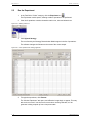
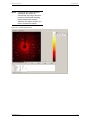
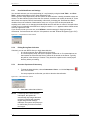
Download apexii user manual 2010 - X-ray Diffraction Texas A & M University

Bruker AXS
APEX2 Release 2010
User Manual
Part Number: DOC-M86-E02078
Publication Date: 13 May 2010
think forward
X-ray Diffraction
APEX2 Software User Manual
This document covers the APEX2 Suite of programs.
References to this document should be shown as DOC-M86-EXX078 APEX2 User Manual.
© 2010 Bruker AXS Inc., 5465 East Cheryl Parkway, Madison, WI 53711. All world rights reserved.
Notice
The information in this publication is provided for reference only. All information contained in this publication is believed to be correct and complete. Bruker AXS Inc. shall not be liable for errors contained herein, nor for incidental or consequential damages in
conjunction with the furnishing, performance, or use of this material. All product specifications, as well as the information contained in this publication, are subject to change without notice.
This publication may contain or reference information and products protected by copyrights or patents and does not convey any
license under the patent rights of Bruker AXS Inc. nor the rights of others. Bruker AXS Inc. does not assume any liabilities arising
out of any infringements of patents or other rights of third parties. Bruker AXS Inc. makes no warranty of any kind with regard to
this material, including but not limited to the implied warranties of merchantability and fitness for a particular purpose.
No part of this publication may be stored in a retrieval system, transmitted, or reproduced in any way, including but not limited to
photocopy, photography, magnetic, or other record without prior written permission of Bruker AXS Inc.
Address comments to:
Technical Publications Department
Bruker AXS Inc.
5465 East Cheryl Parkway
Madison, Wisconsin 53711-5373
USA
All trademarks and registered trademarks are the sole property of their respective owners.
Printed in the U.S.A.
Revision History
Revision
Date
Changes
0
February 2005
Initial release.
1
June 2006
Revised and expanded for APEX2 Version 2.
2
13 May 2010
Revised and expanded.
Bruker Corporation
Bruker AXS Inc.
40 Manning Road
Billerica, MA USA
5465 East Cheryl Parkway
Madison, WI 53711-5373 USA
Phone +1 (978) 663-3660
Fax: +1 (978) 667-5993
Phone +1 (800) 234-XRAY [9729]
Fax +1 (608) 276-3006
E-mail: [email protected]
www.bruker-biosciences.com
E-mail: [email protected]
www.bruker-axs.com
Table of Contents
. . . . . . . . . . . . . . . . . . . . APEX2 Release 2010
1
Notices-i
About this User Manual . . . . . . . . . . . . . . . . . . . . . . . . . . . . . . . . . . . . . . 1-1
1.1
APEX2 Software for Chemical Crystallography . . . . . . . . . . . . . . . . . . . . . . . 1-1
1.2
The Ylid Crystal . . . . . . . . . . . . . . . . . . . . . . . . . . . . . . . . . . . . . . . . . . . . . . . . . 1-2
1.3
Terms and Conventions. . . . . . . . . . . . . . . . . . . . . . . . . . . . . . . . . . . . . . . . . . . 1-3
1.3.1
1.3.2
1.4
Referenced Documentation. . . . . . . . . . . . . . . . . . . . . . . . . . . . . . . . . . . . . . . . 1-5
1.5
X-ray Safety. . . . . . . . . . . . . . . . . . . . . . . . . . . . . . . . . . . . . . . . . . . . . . . . . . . . . 1-6
1.6
Help and Technical Support . . . . . . . . . . . . . . . . . . . . . . . . . . . . . . . . . . . . . . . 1-7
1.6.1
1.6.2
2
Typographical Conventions . . . . . . . . . . . . . . . . . . . . . . . . . . . . . . . . . . . 1-3
Equivalent Terms . . . . . . . . . . . . . . . . . . . . . . . . . . . . . . . . . . . . . . . . . . . 1-3
The “What’s This?” Help Function . . . . . . . . . . . . . . . . . . . . . . . . . . . . . . 1-7
Technical Support from Bruker AXS Service Centers . . . . . . . . . . . . . . . 1-7
APEX2 Software Overview . . . . . . . . . . . . . . . . . . . . . . . . . . . . . . . . . . . . 2-1
2.1
Introduction to Client and Server Functions . . . . . . . . . . . . . . . . . . . . . . . . . . 2-2
2.1.1
2.2
Server Programs . . . . . . . . . . . . . . . . . . . . . . . . . . . . . . . . . . . . . . . . . . . . . . . . 2-3
2.2.1
2.3
Online and Offline Operation . . . . . . . . . . . . . . . . . . . . . . . . . . . . . . . . . . 2-2
The Bruker Instrument Service (BIS). . . . . . . . . . . . . . . . . . . . . . . . . . . . 2-3
Client Programs . . . . . . . . . . . . . . . . . . . . . . . . . . . . . . . . . . . . . . . . . . . . . . . . . 2-4
2.3.1
2.3.2
2.3.3
APEX2 GUI and Modules . . . . . . . . . . . . . . . . . . . . . . . . . . . . . . . . . . . . 2-4
The Bruker Configuration Program (BCP) . . . . . . . . . . . . . . . . . . . . . . . . 2-4
APEX2Server . . . . . . . . . . . . . . . . . . . . . . . . . . . . . . . . . . . . . . . . . . . . . 2-5
2.4
The Sample Database . . . . . . . . . . . . . . . . . . . . . . . . . . . . . . . . . . . . . . . . . . . . 2-6
2.5
License Considerations. . . . . . . . . . . . . . . . . . . . . . . . . . . . . . . . . . . . . . . . . . . 2-6
2.6
The Main Window . . . . . . . . . . . . . . . . . . . . . . . . . . . . . . . . . . . . . . . . . . . . . . . . 2-7
2.6.1
2.6.2
2.6.3
2.6.4
2.6.5
DOC-M86-E02078
The Title Bar . . . . . . . . . . . . . . . . . . . . . . . . . . . . . . . . . . . . . . . . . . . . . . 2-8
The Menu Bar . . . . . . . . . . . . . . . . . . . . . . . . . . . . . . . . . . . . . . . . . . . . . 2-8
The Tool Icon Bar . . . . . . . . . . . . . . . . . . . . . . . . . . . . . . . . . . . . . . . . . 2-10
The Task Bar . . . . . . . . . . . . . . . . . . . . . . . . . . . . . . . . . . . . . . . . . . . . . 2-11
The Task Display Area. . . . . . . . . . . . . . . . . . . . . . . . . . . . . . . . . . . . . . 2-14
iii
Table of Contents
3
APEX2 Software User Manual
Startup and Shutdown . . . . . . . . . . . . . . . . . . . . . . . . . . . . . . . . . . . . . . . 3-1
3.1
User Access . . . . . . . . . . . . . . . . . . . . . . . . . . . . . . . . . . . . . . . . . . . . . . . . . . . . 3-1
3.2
Startup . . . . . . . . . . . . . . . . . . . . . . . . . . . . . . . . . . . . . . . . . . . . . . . . . . . . . . . . . 3-2
3.2.1
3.2.2
3.2.3
3.2.4
3.3
Centering the Crystal . . . . . . . . . . . . . . . . . . . . . . . . . . . . . . . . . . . . . . . . . . . . . 4-1
4.1.1
4.1.2
4.1.3
4.1.4
4.2
Start the Center Crystal Module. . . . . . . . . . . . . . . . . . . . . . . . . . . . . . . . 4-2
Mount the Goniometer Head . . . . . . . . . . . . . . . . . . . . . . . . . . . . . . . . . . 4-2
Center the Crystal on the KAPPA Series II Goniometer . . . . . . . . . . . . . 4-4
Center the Crystal on the D85 Goniometer . . . . . . . . . . . . . . . . . . . . . . 4-10
Checking Crystal Quality . . . . . . . . . . . . . . . . . . . . . . . . . . . . . . . . . . . . . . . . . 4-15
4.2.1
4.2.2
4.2.3
4.2.4
4.2.5
4.2.6
4.2.7
Start the Simple Scans Module . . . . . . . . . . . . . . . . . . . . . . . . . . . . . . .
Set up the Scan . . . . . . . . . . . . . . . . . . . . . . . . . . . . . . . . . . . . . . . . . . .
Use the Resolution Circle Tool . . . . . . . . . . . . . . . . . . . . . . . . . . . . . . .
Use the Line Tool. . . . . . . . . . . . . . . . . . . . . . . . . . . . . . . . . . . . . . . . . .
Plot a Rocking Curve . . . . . . . . . . . . . . . . . . . . . . . . . . . . . . . . . . . . . . .
View Peak Profiles in 3D . . . . . . . . . . . . . . . . . . . . . . . . . . . . . . . . . . . .
Examples of Poor-Quality Crystals . . . . . . . . . . . . . . . . . . . . . . . . . . . .
4-15
4-15
4-17
4-18
4-19
4-20
4-21
Data Collection . . . . . . . . . . . . . . . . . . . . . . . . . . . . . . . . . . . . . . . . . . . . . 5-1
5.1
Create a New Sample . . . . . . . . . . . . . . . . . . . . . . . . . . . . . . . . . . . . . . . . . . . . . 5-2
5.2
Describe the Sample with the Describe Module . . . . . . . . . . . . . . . . . . . . . . . 5-2
5.3
Determining the Unit Cell . . . . . . . . . . . . . . . . . . . . . . . . . . . . . . . . . . . . . . . . . 5-3
5.3.1
5.3.2
5.3.3
5.4
5.5
Start the Determine Unit Cell Module . . . . . . . . . . . . . . . . . . . . . . . . . . . 5-4
Determine the Unit Cell in Automatic Mode. . . . . . . . . . . . . . . . . . . . . . . 5-4
Manual Mode. . . . . . . . . . . . . . . . . . . . . . . . . . . . . . . . . . . . . . . . . . . . . . 5-5
Determining the Data Collection Strategy . . . . . . . . . . . . . . . . . . . . . . . . . . . 5-14
5.4.1
5.4.2
Using the Collect-Style Data Collection Strategy Module . . . . . . . . . . . 5-15
Using the Data Collection Strategy Module . . . . . . . . . . . . . . . . . . . . . . 5-20
Run the Experiment . . . . . . . . . . . . . . . . . . . . . . . . . . . . . . . . . . . . . . . . . . . . . 5-26
5.5.1
5.5.2
5.5.3
iv
Shut Down APEX2 . . . . . . . . . . . . . . . . . . . . . . . . . . . . . . . . . . . . . . . . . 3-3
Shut Down BIS . . . . . . . . . . . . . . . . . . . . . . . . . . . . . . . . . . . . . . . . . . . . 3-3
Crystal Centering and Screening . . . . . . . . . . . . . . . . . . . . . . . . . . . . . . 4-1
4.1
5
3-2
3-2
3-2
3-2
Shutdown . . . . . . . . . . . . . . . . . . . . . . . . . . . . . . . . . . . . . . . . . . . . . . . . . . . . . . 3-3
3.3.1
3.3.2
4
Start BIS . . . . . . . . . . . . . . . . . . . . . . . . . . . . . . . . . . . . . . . . . . . . . . . . .
Start APEX2. . . . . . . . . . . . . . . . . . . . . . . . . . . . . . . . . . . . . . . . . . . . . . .
Log In. . . . . . . . . . . . . . . . . . . . . . . . . . . . . . . . . . . . . . . . . . . . . . . . . . . .
Connect to BIS . . . . . . . . . . . . . . . . . . . . . . . . . . . . . . . . . . . . . . . . . . . .
User-Defined Runs and Settings . . . . . . . . . . . . . . . . . . . . . . . . . . . . . . 5-28
Exiting During Data Collection . . . . . . . . . . . . . . . . . . . . . . . . . . . . . . . . 5-28
Abort the Experiment if Necessary . . . . . . . . . . . . . . . . . . . . . . . . . . . . 5-28
DOC-M86-E02078
APEX2 Software User Manual
6
Data Integration and Scaling . . . . . . . . . . . . . . . . . . . . . . . . . . . . . . . . . . 6-1
6.1
Start the Integrate Images Module . . . . . . . . . . . . . . . . . . . . . . . . . . . . . . . . . . 6-2
6.2
Set the Resolution Limit . . . . . . . . . . . . . . . . . . . . . . . . . . . . . . . . . . . . . . . . . . 6-2
6.3
Select Runs for Integration . . . . . . . . . . . . . . . . . . . . . . . . . . . . . . . . . . . . . . . . 6-3
6.3.1
6.3.2
6.3.3
6.4
6.5
Monitoring Integration Progress with SaintChart . . . . . . . . . . . . . . . . . . 6-10
Examine the Integration Results. . . . . . . . . . . . . . . . . . . . . . . . . . . . . . . . . . . 6-13
6.7.1
6.7.2
6.8
Integration Options Controls . . . . . . . . . . . . . . . . . . . . . . . . . . . . . . . . . . 6-8
Start the Integration . . . . . . . . . . . . . . . . . . . . . . . . . . . . . . . . . . . . . . . . . . . . . 6-10
6.6.1
6.7
Refinement Options Controls . . . . . . . . . . . . . . . . . . . . . . . . . . . . . . . . . 6-6
Set the Integration Options . . . . . . . . . . . . . . . . . . . . . . . . . . . . . . . . . . . . . . . . 6-7
6.5.1
6.6
Browse for Runs . . . . . . . . . . . . . . . . . . . . . . . . . . . . . . . . . . . . . . . . . . . 6-3
Import Runs from Experiment . . . . . . . . . . . . . . . . . . . . . . . . . . . . . . . . . 6-4
Modifying Integration Run Lists . . . . . . . . . . . . . . . . . . . . . . . . . . . . . . . . 6-4
Set the Refinement Options . . . . . . . . . . . . . . . . . . . . . . . . . . . . . . . . . . . . . . . 6-5
6.4.1
Overall Rsym and Coverage Statistics . . . . . . . . . . . . . . . . . . . . . . . . . 6-13
Unconstrained Unit Cell Refinement . . . . . . . . . . . . . . . . . . . . . . . . . . . 6-14
Scaling Data . . . . . . . . . . . . . . . . . . . . . . . . . . . . . . . . . . . . . . . . . . . . . . . . . . . 6-15
6.8.1
6.8.2
6.8.3
6.8.4
6.8.5
6.8.6
7
Table of Contents
Start the Scale Module . . . . . . . . . . . . . . . . . . . . . . . . . . . . . . . . . . . . .
Set Up the Scale Operation . . . . . . . . . . . . . . . . . . . . . . . . . . . . . . . . . .
Refine the Parameters. . . . . . . . . . . . . . . . . . . . . . . . . . . . . . . . . . . . . .
Refine the Error Model . . . . . . . . . . . . . . . . . . . . . . . . . . . . . . . . . . . . .
Examine the Diagnostic Plots . . . . . . . . . . . . . . . . . . . . . . . . . . . . . . . .
Close the Scale Module. . . . . . . . . . . . . . . . . . . . . . . . . . . . . . . . . . . . .
6-16
6-16
6-18
6-20
6-21
6-23
Examining Data . . . . . . . . . . . . . . . . . . . . . . . . . . . . . . . . . . . . . . . . . . . . . 7-1
7.1
Using the Space Groups and Statistics Module . . . . . . . . . . . . . . . . . . . . . . . 7-2
7.1.1
7.1.2
7.1.3
7.1.4
7.1.5
7.1.6
7.1.7
7.1.8
7.1.9
7.1.10
7.2
Determining the Space Group with XPREP . . . . . . . . . . . . . . . . . . . . . . . . . . 7-11
7.2.1
7.2.2
7.2.3
7.2.4
DOC-M86-E02078
Start the Space Groups and Statistics Module. . . . . . . . . . . . . . . . . . . . . 7-2
Set Up the Determination Parameters. . . . . . . . . . . . . . . . . . . . . . . . . . . 7-2
Examine the Lattice Exceptions . . . . . . . . . . . . . . . . . . . . . . . . . . . . . . . 7-3
Choose a Space Group . . . . . . . . . . . . . . . . . . . . . . . . . . . . . . . . . . . . . . 7-4
Examine the Reflection Statistics . . . . . . . . . . . . . . . . . . . . . . . . . . . . . . 7-5
Check the Unit Cell Contents . . . . . . . . . . . . . . . . . . . . . . . . . . . . . . . . . 7-7
Set Up the Output File . . . . . . . . . . . . . . . . . . . . . . . . . . . . . . . . . . . . . . . 7-8
Examine Cell Information . . . . . . . . . . . . . . . . . . . . . . . . . . . . . . . . . . . . 7-9
Examine Diagnostics . . . . . . . . . . . . . . . . . . . . . . . . . . . . . . . . . . . . . . . 7-10
Exit the Space Groups and Statistics Module . . . . . . . . . . . . . . . . . . . . 7-10
Determine the Space Group . . . . . . . . . . . . . . . . . . . . . . . . . . . . . . . . .
Examine Reflection Statistics . . . . . . . . . . . . . . . . . . . . . . . . . . . . . . . .
Prepare an Output File . . . . . . . . . . . . . . . . . . . . . . . . . . . . . . . . . . . . .
Quit XPREP. . . . . . . . . . . . . . . . . . . . . . . . . . . . . . . . . . . . . . . . . . . . . .
7-12
7-14
7-16
7-17
v
Table of Contents
APEX2 Software User Manual
7.3
Create Simulated Precession Images . . . . . . . . . . . . . . . . . . . . . . . . . . . . . . 7-18
8
Structure Solution and Refinement. . . . . . . . . . . . . . . . . . . . . . . . . . . . . 8-1
8.1
Using AUTOSTRUCTURE . . . . . . . . . . . . . . . . . . . . . . . . . . . . . . . . . . . . . . . . . 8-1
8.1.1
8.1.2
8.1.3
8.2
Solving the Structure with the Structure Solution Module. . . . . . . . . . . . . . . 8-4
8.2.1
8.2.2
8.2.3
8.3
9.1
Preparing for Report Generation . . . . . . . . . . . . . . . . . . . . . . . . . . . . . . . . . . . 9-1
9.2
Using the Module . . . . . . . . . . . . . . . . . . . . . . . . . . . . . . . . . . . . . . . . . . . . . . . . 9-2
9.3
9.4
Saving the CIF-Formatted Report . . . . . . . . . . . . . . . . . . . . . . . . . . . . . . 9-5
Adding Additional Information to the Report . . . . . . . . . . . . . . . . . . . . . . . . . 9-6
9.5.1
9.5.2
9.5.3
9.6
Saving the HTML-Formatted Report . . . . . . . . . . . . . . . . . . . . . . . . . . . . 9-4
Creating a Report for Submission to Acta Crystallographica . . . . . . . . . . . . 9-5
9.4.1
9.5
Starting the Module . . . . . . . . . . . . . . . . . . . . . . . . . . . . . . . . . . . . . . . . . 9-2
Choosing a Template File . . . . . . . . . . . . . . . . . . . . . . . . . . . . . . . . . . . . 9-3
Creating an HTML-Formatted Report for Online or Print Distribution . . . . . 9-4
9.3.1
Adding Information from a .CIF File. . . . . . . . . . . . . . . . . . . . . . . . . . . . . 9-7
Adding the Run List . . . . . . . . . . . . . . . . . . . . . . . . . . . . . . . . . . . . . . . . . 9-8
Adding Additional Information . . . . . . . . . . . . . . . . . . . . . . . . . . . . . . . . . 9-9
Report Sections . . . . . . . . . . . . . . . . . . . . . . . . . . . . . . . . . . . . . . . . . . . . . . . . 9-11
9.6.1
9.6.2
9.6.3
9.6.4
9.6.5
9.6.6
vi
Refining the Structure in XSHELL . . . . . . . . . . . . . . . . . . . . . . . . . . . . . . 8-9
Labelling the Atoms . . . . . . . . . . . . . . . . . . . . . . . . . . . . . . . . . . . . . . . . 8-12
Refining the Model. . . . . . . . . . . . . . . . . . . . . . . . . . . . . . . . . . . . . . . . . 8-13
Refining for Publication with XSHELL . . . . . . . . . . . . . . . . . . . . . . . . . . 8-21
Creating a Publication-Quality Image . . . . . . . . . . . . . . . . . . . . . . . . . . 8-22
Using the Report Generation Module . . . . . . . . . . . . . . . . . . . . . . . . . . . 9-1
9.2.1
9.2.2
10
Direct Methods Options . . . . . . . . . . . . . . . . . . . . . . . . . . . . . . . . . . . . . . 8-6
Dual-Space Methods Options . . . . . . . . . . . . . . . . . . . . . . . . . . . . . . . . . 8-6
Patterson Methods Options . . . . . . . . . . . . . . . . . . . . . . . . . . . . . . . . . . . 8-6
Refining the Structure with the Structure Refinement Module . . . . . . . . . . . 8-7
8.3.1
8.3.2
8.3.3
8.3.4
8.3.5
9
Before you Begin . . . . . . . . . . . . . . . . . . . . . . . . . . . . . . . . . . . . . . . . . . . 8-1
Solving the Structure . . . . . . . . . . . . . . . . . . . . . . . . . . . . . . . . . . . . . . . . 8-2
Automatically Solving and Refining the Structure . . . . . . . . . . . . . . . . . . 8-3
“Report” Tab. . . . . . . . . . . . . . . . . . . . . . . . . . . . . . . . . . . . . . . . . . . . . .
“Atoms” Tab . . . . . . . . . . . . . . . . . . . . . . . . . . . . . . . . . . . . . . . . . . . . . .
“Bond Lengths” Tab . . . . . . . . . . . . . . . . . . . . . . . . . . . . . . . . . . . . . . . .
Bond Angles . . . . . . . . . . . . . . . . . . . . . . . . . . . . . . . . . . . . . . . . . . . . .
“Torsion Angles” Tab . . . . . . . . . . . . . . . . . . . . . . . . . . . . . . . . . . . . . . .
“Miscellaneous” Tab. . . . . . . . . . . . . . . . . . . . . . . . . . . . . . . . . . . . . . . .
9-11
9-12
9-13
9-14
9-15
9-16
Appendices . . . . . . . . . . . . . . . . . . . . . . . . . . . . . . . . . . . . . . . . . . . . . . . 10-1
DOC-M86-E02078
APEX2 Software User Manual
10.1
Table of Contents
Using BCP with APEX2 . . . . . . . . . . . . . . . . . . . . . . . . . . . . . . . . . . . . . . . . . . 10-2
10.1.1
10.1.2
10.1.3
10.1.4
10.1.5
Start BCP . . . . . . . . . . . . . . . . . . . . . . . . . . . . . . . . . . . . . . . . . . . . . . . .
Select a Connection Mode . . . . . . . . . . . . . . . . . . . . . . . . . . . . . . . . . .
Parameter Menus . . . . . . . . . . . . . . . . . . . . . . . . . . . . . . . . . . . . . . . . .
Change the Detector’s Beam Center. . . . . . . . . . . . . . . . . . . . . . . . . . .
Collect a Dark Current Correction . . . . . . . . . . . . . . . . . . . . . . . . . . . . .
10-2
10-2
10-2
10-3
10-5
10.2
Set Default Orientation Matrix Scans in the bn-config.py File . . . . . . . . . . . 10-6
10.3
Face Indexing with the Crystal Faces Module . . . . . . . . . . . . . . . . . . . . . . . . 10-7
10.3.1
10.3.2
10.3.3
10.3.4
10.3.5
10.3.6
10.4
The Reciprocal Lattice Viewer Module . . . . . . . . . . . . . . . . . . . . . . . . . . . . . 10-15
10.4.1
10.4.2
10.4.3
10.4.4
10.4.5
10.5
Starting the Crystal Faces Module. . . . . . . . . . . . . . . . . . . . . . . . . . . . . 10-7
Collecting a Video Zip Stream . . . . . . . . . . . . . . . . . . . . . . . . . . . . . . . . 10-7
The Crystal Faces Module Interface . . . . . . . . . . . . . . . . . . . . . . . . . . . 10-9
Specifying Crystal Faces . . . . . . . . . . . . . . . . . . . . . . . . . . . . . . . . . . . 10-11
Editing the Face List . . . . . . . . . . . . . . . . . . . . . . . . . . . . . . . . . . . . . . 10-13
Scaling with Face Indices . . . . . . . . . . . . . . . . . . . . . . . . . . . . . . . . . . 10-14
Start the Reciprocal Lattice Viewer Module . . . . . . . . . . . . . . . . . . . . .
Views and Tools. . . . . . . . . . . . . . . . . . . . . . . . . . . . . . . . . . . . . . . . . .
Defining Groups. . . . . . . . . . . . . . . . . . . . . . . . . . . . . . . . . . . . . . . . . .
Measuring Distances and Angles . . . . . . . . . . . . . . . . . . . . . . . . . . . .
Writing a .p4p File . . . . . . . . . . . . . . . . . . . . . . . . . . . . . . . . . . . . . . . .
10-15
10-15
10-28
10-30
10-30
Using CELL_NOW . . . . . . . . . . . . . . . . . . . . . . . . . . . . . . . . . . . . . . . . . . . . . 10-31
10.5.1 Running CELL_NOW on a List of Reflections . . . . . . . . . . . . . . . . . . . 10-31
10.5.2 CELL_NOW Output . . . . . . . . . . . . . . . . . . . . . . . . . . . . . . . . . . . . . . . 10-36
10.6
Configuring the Suite. . . . . . . . . . . . . . . . . . . . . . . . . . . . . . . . . . . . . . . . . . . 10-37
10.6.1
10.6.2
10.6.3
10.6.4
10.6.5
Index
The bn-config Configuration File . . . . . . . . . . . . . . . . . . . . . . . . . . . . .
Global, User, and Sample-specific Variables. . . . . . . . . . . . . . . . . . . .
Configuration File Examples . . . . . . . . . . . . . . . . . . . . . . . . . . . . . . . .
Functionality Groups in the Configuration File. . . . . . . . . . . . . . . . . . .
Configuration File Variables. . . . . . . . . . . . . . . . . . . . . . . . . . . . . . . . .
10-37
10-38
10-39
10-41
10-42
. . . . . . . . . . . . . . . . . . . . . . . . . . . . . . . . . . . . . . . . . . . . . . . . . . . . . . .Index-1
DOC-M86-E02078
vii
Table of Contents
APEX2 Software User Manual
This page intentionally left blank.
viii
DOC-M86-E02078
1
About this User Manual
1.1
APEX2 Software for Chemical Crystallography
Figure 1.1 — APEX2 software (Integrate Images module shown)
APEX2 is Bruker’s comprehensive software suite for single-crystal X-ray diffraction. APEX2, combined
with Bruker’s X-ray diffractometer hardware, provides the tools for complete small-molecule structure
determination. The software provides the highest-quality data: from acquisition, collection, integration
and scaling, through structure solution and refinement, through report generation.
DOC-M86-E02078
1-1
About this User Manual
APEX2 User Manual
APEX2 redefines user interaction with the crystallographic experiment. The user interface guides the
user through the complete experiment with minimal user input and maximal graphical feedback. APEX2
lets the user focus on the structure determination at hand and does not require any knowledge of
instrument geometry or data collection strategies. APEX2 is easy to use for the novice, but has all of
the features required by expert crystallographers.
The software features a client/server architecture that provides for remote control of—and access
to—the instrumentation.
Optional software modules for APEX2 include XRD2 Eval for powder diffraction pattern integration, and
AUTOSTRUCTURE for completely-automated structure solution.
1.2
The Ylid Crystal
The compound used was 2-dimethylsulfuranylidene-1,3-indanedione (abbreviated “ylid”):
C11H10O2S
More information on the ylid crystal is available in the article “Polymorphism and History of
2-Dimethylsufuranylidene-1,3-indanedione (YLID)”, Ilia A. Guzei, Galina A. Bikzhanova, Lara C.
Spencer, Tatiana V. Timofeeva, Tiffany L. Kinnibrugh and Charles F. Campana. Cryst. Growth Des.,
2008, 8 (7), pp. 2411–2418, DOI: 10.1021/cg701260p.
Figure 1.2 — Ylid crystal structure
1-2
DOC-M86-E02078
APEX2 User Manual
About this User Manual
1.3
Terms and Conventions
1.3.1
Typographical Conventions
Table 1.1 shows typographical conventions used to help you quickly locate and identify information in
this document.
Table 1.1 —
Typographical conventions
Convention
Usage
boldface
Software user interface controls (such as icons, menu items, and buttons) to be selected as part
of the current procedure.
italics
New terms and words requiring emphasis.
monospace
Information read from or entered into a field or command prompt.
>
Navigation through a hierarchical menu. For example, “Choose Start > Programs > Bruker AXS
> BIS” describes navigating Windows’ menus from Start to Programs to Bruker AXS to BIS.
[square brackets]
Keyboard input.
1.3.2
Equivalent Terms
Frame/Image
In 2-dimensional X-ray diffraction, the terms frame and image refer to the same 2-dimensional view of
the diffraction pattern.
Greek and Roman Text
This document uses scientific terminology that may be rendered in Greek text. However, this document
follows a convention of using Roman text to the greatest extent possible.
Table 1.2 —
Greek and Roman Text
Greek
Roman
2θ
2theta
ω
omega
φ
phi
χ
chi
κ
kappa
DOC-M86-E02078
1-3
About this User Manual
APEX2 User Manual
Notices: Danger, Caution, and Note
This document contains notices that must be observed to ensure personal safety, as well as to protect
the product and connected equipment. These notices are highlighted as follows according to the level
of danger.
!
!
!
!
DANGER
WARNING
The word “DANGER” alerts you to an immediate
or potential hazard that can result in death,
severe personal injury, or substantial property
damage.
CAUTION
WARNING
The word “CAUTION” alerts you to a potential
practice or condition that could result in minor
personal injury or damage to the product or
property.
NOTE:
1-4
The word “NOTE” in bold capital letters
draws your attention to particularly
important information on the product or
handling of the product, or to a
particular part of the product
documentation.
DOC-M86-E02078
APEX2 User Manual
1.4
About this User Manual
Referenced Documentation
The following Table contains a list of documentation referenced by this document. It is necessary to
have this additional documentation available as you work with this document. In the documents’ part
numbers, a variable revision number is indicated by a letter “X”. Always use the most current revisions
available.
All of the documents shown in the Table may be found at Bruker AXS’ comprehensive support site
www.brukersupport.com, or on the Online Documentation CD-ROM that accompanies the shipment.
Table 1.3 —
Referenced documentation
Part Number
Title
DOC-269-0159XX
SHELXTL Software Reference Manual
DOC-269-0175XX
SAINT Software Reference Manual
DOC-269-0228XX
VIDEO Installation Notes
DOC-M86-EXX010
COSMO Installation Notes
DOC-M86-EXX024
D8 and PLATFORM Microscope Focus and Sample Alignment Procedure
DOC-M86-EXX043
BCP and BIS Installation Notes
DOC-M86-EXX045
RLATT User Manual
DOC-M86-EXX087
APEX2 and PROTEUM2 Installation Notes
DOC-M86-EXX092
User Manager User Manual
DOC-M86-EXX112
COSMATIC Fixed-Chi Geometry Hardware Profile Procedure
DOC-M86-EXX113
COSMATIC Kappa Geometry Hardware Profile Procedure
DOC-M88-EXX099
License Manager User Manual
DOC-M86-E02078
1-5
About this User Manual
1.5
!
APEX2 User Manual
X-ray Safety
!
DANGER
WARNING
X-ray equipment produces potentially harmful
radiation and can be dangerous to anyone in the
equipment’s vicinity unless safety precautions
are completely understood and implemented. All
persons designated to operate or perform
maintenance on this instrument must be fully
trained on the nature of radiation, X-ray
generating equipment, and radiation safety. All
users of the X-ray equipment are required to
accurately monitor their exposure to X-rays by
proper use of X-ray dosimeters.
For safety issues related to operation and maintenance of your particular X-ray generator,
diffractometer, and shield enclosure, please refer to the manufacturer’s operation manuals or to your
Radiation Safety Officer. The user is responsible for compliance with local safety regulations.
1-6
DOC-M86-E02078
APEX2 User Manual
About this User Manual
1.6
Help and Technical Support
1.6.1
The “What’s This?” Help Function
Context-based help is available at any time within the program by simply clicking the “What’s This?”
help icon:
Figure 1.3 — “What’s This?” help icon
After clicking the icon, click on any window or field to obtain detailed help in a pop-up window.
The “What’s This?” help function can also be invoked at any time by pressing [Shift]+[F1].
1.6.2
Technical Support from Bruker AXS Service Centers
You are invited to contact Bruker AXS whenever there are problems or questions related to the system.
Before contacting Bruker AXS, please:
!
•
If you suspect a software problem, determine the system’s software version.
•
Record any error messages that appear.
•
If possible, determine conditions and steps that recreate the problem.
!
CAUTION
WARNING
Failure to refer instrument servicing to qualified
Bruker personnel may result in injury or property
damage!
North American Service Center Contact Information
Table 1.4 —
Bruker AXS North American Service Center contact information
Bruker AXS North American Service Center
Address:
Bruker AXS Inc.
Customer Support
5465 East Cheryl Parkway
Madison, WI 53711-5373
USA
Toll-free telephone:
1 (800) 234-XRAY [9729]
Direct line:
1 (608) 276-3087
Fax:
1 (608) 276-3015
E-mail:
[email protected]
Web:
http://www.bruker-axs.com
Outside North America
Outside North America, contact your local Bruker AXS Service Center.
DOC-M86-E02078
1-7
About this User Manual
APEX2 User Manual
This page intentionally left blank.
1-8
DOC-M86-E02078
2
APEX2 Software Overview
From a software and operational viewpoint, the APEX2 software controls all operations—from crystal
screening to report generation—for a typical crystallography study.
This is a complete departure from the older, functionally-separate programs SMART, SAINTPLUS, and
SHELXTL. Enhanced versions of the proven and widely-accepted algorithms used by these programs
(e.g., SAINT, SADABS, XPREP, XS, XM, XL, etc.) form the foundation of the APEX2 software.
DOC-M86-E02078
2-1
APEX2 Software Overview
2.1
APEX2 User Manual
Introduction to Client and Server Functions
The various programs within the Bruker Single-Crystal and Powder Diffraction Suite have a
client-server relationship (Figure 2.1), in which the server program (BIS) executes commands given by
one of several client programs (APEX2, APEX2Server, or BCP).
Figure 2.1 — Client and server relationships
2.1.1
Online and Offline Operation
The Suite can operate in online or offline mode.
In online mode, the Suite uses BIS to communicate with the instrument for performing experiments. To
work in online mode, you must start BIS, your Suite program (i.e., APEX2). BIS will also start VIDEO
when needed.
In offline mode, the Suite program is not connected to the instrument, but is still able to analyze and
interpret existing data. To work in offline mode, you only need to start your Suite program.
2-2
DOC-M86-E02078
APEX2 User Manual
2.2
Server Programs
2.2.1
The Bruker Instrument Service (BIS)
APEX2 Software Overview
BIS acts as a server to the client programs, providing a link between the hardware and software. Once
a connection is established, BIS executes hardware commands sent by the client programs. BIS can
also be used as a service tool, displaying diagnostic messages during operation.
Figure 2.2 — BIS main window
DOC-M86-E02078
2-3
APEX2 Software Overview
2.3
Client Programs
2.3.1
APEX2 GUI and Modules
APEX2 User Manual
APEX2 is the main program that controls experiments and analyzes data. The user works with APEX2
though a variety of plug-ins, or modules, for different aspects of an experiment. The Suite includes a
sample database that stores relevant data from each step in the experiment.
2.3.2
The Bruker Configuration Program (BCP)
BCP is a client program for BIS. It is used to configure BIS, as well as provide instrument control and
alignment tools.
In BCP’s main window (Figure 2.3), specific hardware parameters can be updated. BCP writes these
values to the configuration file BrukerInstrument.ini, which is used by BIS. When changes are saved in
BCP, BIS automatically reads in the new values.
See DOC-M86-EXX043 BCP and BIS Installation Notes, in addition to BCP’s online help, for more
information.
Figure 2.3 — BCP main window (Configuration screen)
2-4
DOC-M86-E02078
APEX2 User Manual
2.3.3
APEX2 Software Overview
APEX2Server
APEX2Server is operated on the computer that controls the instrument. It provides functionality for
quickly centering a crystal and determining its diffraction quality.
APEX2Server contains two main modules: “Center Crystal” and “Simple Scans” (see Figure 2.4).
Figure 2.4 — APEX2Server’s “Simple Scans” module
DOC-M86-E02078
2-5
APEX2 Software Overview
2.4
APEX2 User Manual
The Sample Database
The Sample Database is used for the storage of data generated by the Suite. It is designed to
transparently handle data from all of the Suite’s modules without intervention from the user.
The sample database is used internally by the Suite and is not available for user customization or
manipulation. It is automatically started when the computer starts up, and it is automatically stopped
before the computer shuts down.
2.5
License Considerations
You need a software license to activate your purchased software packages, options, and/or features.
The Suite requires a valid license file to operate. This file, “bn-license.dat”, must be present in the root
directory of drive C:\ for the software to start properly.
If the license file is not present or has expired, an error window will appear when you try to start your
Suite program (i.e., APEX2). This window prompts you to run the License Manager application to obtain
a valid license for the Suite.
For more information on licenses and License Manager, refer to DOC-M88-EXX099 License Manager
User Manual.
2-6
DOC-M86-E02078
APEX2 User Manual
2.6
APEX2 Software Overview
The Main Window
The APEX2 graphical user interface (GUI) has one main window (Figure 2.5).
Figure 2.5 — Main window diagram
The main window is divided into five sections:
NOTE:
•
Title Bar
•
Menu Bar
•
Tool Icon Bar
•
Task Bar
•
Task Display Area
Throughout the interface, input fields
with pink backgrounds indicate invalid
entries. Disabled (i.e., grayed-out)
fields indicate that a feature is not
available (i.e., not supported or
dependent upon the instrument
configuration).
DOC-M86-E02078
2-7
APEX2 Software Overview
2.6.1
APEX2 User Manual
The Title Bar
The Title Bar displays the software name and version, user name, sample, license type, and active
module. The right-hand edge of the Title Bar also contains the three Windows buttons
minimizing, restoring, and closing the main window.
2.6.2
for
The Menu Bar
The Menu Bar provides drop-down menus for a variety of file operations, image tools, and help files.
An icon for the currently-active module appears on the left-hand side of the Menu Bar. Clicking on this
icon allows you to minimize, restore, resize, close, or move the currently-active window.
The Sample Menu
Figure 2.6 — Sample menu
Table 2.1 —
Sample menu commands
Sample menu command
Description
Login...
Opens a window for logging into the Sample Database using your username and password.
Logout
Logs out of the Sample Database.
Change Password...
Opens a dialog for changing your Sample Database password.
New...
Opens a dialog for creating a new sample in the Sample Database.
Open...
Opens a previously-saved sample.
Reopen
Reopens a recently-opened sample.
Save
Saves the current sample.
Close
Closes the current sample.
Archive
Restore Archive...
Restores an archived sample from a .zip file or CD.
Archive Sample...
Archives the current sample to a .zip file or CD.
Delete Samples...
Deletes samples from the Sample Database.
Show Notes...
Opens the “Sample Notes” window.
Import
Allows you to import crystal information contained in a .p4p or .spin file into the Sample
Database.
Export
Allows you to export crystal data for the current sample as an .xml or .p4p file.
Run Command...
Opens a command prompt window.
Exit
Exits the application. This menu item has the same function as the
2-8
button.
DOC-M86-E02078
APEX2 User Manual
APEX2 Software Overview
The Instrument Menu
Figure 2.7 — Instrument menu
Table 2.2 —
Instrument menu commands
Instrument menu command
Description
Connect...
Opens a connection to BIS.
Disconnect
If connected, disconnects from BIS.
Show Status...
Opens a window showing a summary of the current status of
the instrument and the program’s connection to it.
Toggle Shutter
Instructs BIS to send a shutter open or close command to the
instrument. If all interlocks and safety circuits are satisfied, the
shutter will open and close.
Abort...
Aborts all pending instrument operations.
The Windows Menu
Figure 2.8 — Windows menu
Table 2.3 —
Windows menu command
Windows menu command
Description
Window selection
Displays a list of active windows. Any of these windows may
be brought to the front by clicking its title.
The Help Menu
Figure 2.9 — Help menu
Table 2.4 —
Help menu command
Help menu command
Description
About APEX2...
Displays APEX2’s version and copyright information.
DOC-M86-E02078
2-9
APEX2 Software Overview
2.6.3
APEX2 User Manual
The Tool Icon Bar
Some icons on the Tool Icon Bar provide shortcuts to the options available through the Menu Bar.
Table 2.5 —
Icon
Tool Icon Bar: menu bar shortcuts
Description
Creates a new entry in the Sample Database.
Opens an existing entry in the Sample Database.
Saves the current information to the Sample Database.
Shows the “Sample Notes” window
Stops any instrument activity.
“What’s this?” Context-sensitive help.
Other icons on the Tool Icon Bar are visible only when a frame is displayed.
Table 2.6 —
Icon
Tool Icon Bar: displayed frame controls
Description
Shows the currently-displayed frame’s filename. Click the drop-down triangle to choose
previously-displayed frames.
Opens a frame using a browse dialog.
Displays the first frame in a run.
Displays previous frame.
Sequentially displays frames in reverse as a movie.
If displaying frames as a movie, stops the movie.
Sequentially displays frames as a movie.
Displays the next frame.
Displays the last frame in a run.
Adjusts the rate of display when viewing frames as a movie.
Displays frames from the next lower-numbered run.
Displays frames from the next higher-numbered run.
Draws a resolution circle.
Draws a plotting line. The plot appears below the image.
Selects a region of the frame.
2 - 10
DOC-M86-E02078
APEX2 User Manual
2.6.4
APEX2 Software Overview
The Task Bar
The Task Bar gives you access to all of the modules available in the Suite.
NOTE:
If the Task Bar is not visible, there is no
open sample. Choose Sample >
New... or Sample > Open... to open or
create a new sample.
Table 2.7 —
“Setup” category
Icon
Table 2.8 —
Description
Describe
Specify crystal size, color, shape, etc.
Center Crystal
Manual and motorized crystal centering.
Simple Scans
Provides tools for rapid crystal screening using phi and omega scans.
“Evaluate” category
Icon
Table 2.9 —
Name
Name
Description
Determine Unit Cell
Determine unit cell and Bravais lattice type.
Transform Unit Cell
Transform a unit cell.
Reciprocal Lattice Viewer
3D visualization of the lattice projected in reciprocal space.
View Images
View and analyze diffraction images.
“Collect” category
Icon
Name
Description
Data collection strategy
Data collection strategy as in Collect.
Data Collection Strategy
Simulate data collection and determine strategy.
Experiment
Sequence editor for data collection experiments.
Oriented Scans
Measure diffraction frames with the crystal aligned along axes.
Table 2.10 — “Integrate” category
Icon
Name
Description
Integrate Images
Integrate diffraction data.
Table 2.11 — “Scale” category
Icon
DOC-M86-E02078
Name
Description
Crystal Faces
Determine Miller indices and distances of single-crystal faces.
Scale
Scale intensities and perform absorption correction.
2 - 11
APEX2 Software Overview
APEX2 User Manual
Table 2.12 — “Examine Data” category
Icon
Name
Description
Space Groups and Statistics
Dataset analysis and manipulation.
Compare Unit Cells
Compare unit cells to find twin laws.
Precession Images
Create precession images based on measured frames.
Diffraction Space Viewer
Create a 3D view in reciprocal space based on measured frames.
Space Group Determination
Run XPREP.
Find a Reflection
Find a reflection in measured frames.
Table 2.13 — “Solve Structure” category
Icon
Name
Description
AUTOSTRUCTURE
Automatic solution and refinement with minimum user input.
Structure Solution
Solve the structure.
View Molecule
Visualize the molecule in 3D.
Table 2.14 — “Refine Structure” category
Icon
Name
Description
Structure Refinement
Run XP, XL, or XSHELL.
Table 2.15 — “Report” category
Icon
Name
Description
Generate Report
Use Bruker’s automatic report generation system.
Generate Report
Run XCIF to generate a report.
Table 2.16 — “PILOT” category
Icon
Name
Description
XRD² Eval
Display and integrate single and multiple frames.
Table 2.17 — “Instrument” category
Icon
2 - 12
Name
Description
System Calibration
Make calibration measurements.
Unwarp and Convert Images
Convert frames between formats.
Play Tic Tac Toe
Play a game of Tic Tac Toe!
DOC-M86-E02078
APEX2 User Manual
APEX2 Software Overview
Stack Bar and Tree View
Right-click in the Task Bar to choose one of two views: Stack Bar or Tree View.
Figure 2.10 —Stack Bar view
In Stack Bar view, click one of the Task Bar categories to display only the icons belonging to that
category. All other Task Bar icons will be hidden.
Figure 2.11 — Tree view
In Tree View, categories may be expanded to display their Task Bar icons by clicking the plus or minus
sign next to the category name.
DOC-M86-E02078
2 - 13
APEX2 Software Overview
2.6.5
APEX2 User Manual
The Task Display Area
The Task Display Area is the main area for tasks, user input, and selected output. This area displays
images and other output from the modules.
NOTE:
In APEX2 Version 2, XSHELL
refinement and XCIF report generation
do not use the Task Display Area; they
open in new windows. All other
modules open in APEX2’s Task Display
Area.
Figure 2.12 —Task Display Area showing the Data Collection Strategy module
2 - 14
DOC-M86-E02078
3
Startup and Shutdown
3.1
User Access
Bruker software allows different user accounts to have different levels of access to the instrument:
•
Service
•
Security
•
Administrator
•
User
•
Non-user
You need “Bruker Instrument Administrator” rights to run BCP and “Bruker Instrument User” rights to
run programs from the Suite. Typically, your system administrator will already have your user account
configured or you will be using the default accounts as provided by Bruker AXS.
DOC-M86-E02078
3-1
Startup and Shutdown
3.2
Startup
3.2.1
Start BIS
1.
APEX2 User Manual
From the Windows Task Bar, choose Start > Programs > Bruker AXS >
Administration > BIS.
The BIS main window opens.
2.
3.2.2
Start APEX2
1.
3.2.3
If you are asked to confirm any system parameters, do so and click OK.
From the Windows Task Bar, choose Start > Programs > Bruker AXS > APEX2.
Log In
1.
At the “Login” dialog, enter your user name and password (as shipped by Bruker AXS,
the default account is guest with password guest). Click OK.
Figure 3.1 — “Login” dialog
NOTE:
If your setup does not require individual
login accounts, you can configure the
software to automatically log into a
specified account.
3.2.4
Connect to BIS
1.
To use the software in online mode, choose Instrument > Connect....
The “Instrument Connection” dialog appears.
2.
Enter the instrument host name (the dialog shows the default host). Click Connect.
Figure 3.2 — “Instrument Connection” dialog
3-2
DOC-M86-E02078
APEX2 User Manual
Startup and Shutdown
3.3
Shutdown
3.3.1
Shut Down APEX2
1.
Log out of the Sample Database by choosing Sample > Logout.
2.
In the “Closing Sample” window, choose whether to save or discard the changes made
to the Sample Database.
Figure 3.3 — “Closing Sample” window
NOTE:
The “Closing Sample” window appears
even if no apparent changes were
made to the Sample Database,
because the date and time of the last
access are held in the Sample
Database and differ from the current
date and time.
3.
Choose Sample > Exit.
APEX2 closes.
3.3.2
Shut Down BIS
NOTE:
If BIS is running, it will prevent your
computer from shutting down or
rebooting.
1.
Click the Exit button in the upper right-hand corner of BIS’ main window. You may be
asked to place the generator into standby mode.
2.
At the confirmation dialog, click OK.
BIS closes.
DOC-M86-E02078
3-3
Startup and Shutdown
APEX2 User Manual
This page intentionally left blank.
3-4
DOC-M86-E02078
4
Crystal Centering and Screening
4.1
Centering the Crystal
To obtain accurate unit cell dimensions and collect high-quality data, position the crystal in the center of
the X-ray beam and maintain this position for the entire experiment.
Your video microscope should be aligned so that the VIDEO software’s reticle coincides with the
goniometer center (for instructions on aligning the microscope to the center of the instrument, see
DOC-M86-EXX024 Microscope Focus and Sample Alignment). If the reticle does not coincide with the
goniometer center, you can still center the crystal. A successfully-centered crystal stays in the same
place in the microscope’s field of view in all orientations.
Also, the centering process can be greatly helped by lighting both the sample and background for
maximum contrast.
NOTE:
Use the thin end of the goniometer
wrench to unlock the X, Y and Z locks
at the beginning of the centering
process and to lock them at the end.
Locking needs only a very slight touch.
The other end of the wrench is used to
move the adjustment sleds. Do not
overtighten the locks.
NOTE:
Centering is often easier if the crystal is
rotated to give a good view before the
actual centering process is started
(e.g., down an edge for a plate). To do
this, drive to the initial centering
position, loosen the crystal mounting
screw, rotate the crystal to a suitable
orientation, and then tighten the screw
again.
DOC-M86-E02078
4-1
Crystal Centering and Screening
4.1.1
APEX2 User Manual
Start the Center Crystal Module
1.
Under the “Setup” category in the Task Bar, click the Center Crystal icon
.
The Center Crystal module opens.
4.1.2
!
Mount the Goniometer Head
1.
Open the enclosure doors.
2.
In the Center Crystal Module, click Mount to drive the goniometer to a convenient
position for mounting the goniometer head.
3.
Carefully remove the goniometer head containing the crystal from its case.
!
CAUTION
WARNING
Use extreme care when handling the goniometer
head to prevent damage to the crystal on the end
of the small glass fiber.
4.
Place the goniometer head onto its base on the phi drive. Line up the slot on the bottom
of the goniometer head with the pin on the mounting base (Figure 4.1).
Figure 4.1 — Goniometer head bottom
5.
4-2
Screw the goniometer head collar to the base so that the head does not move. Do not
overtighten it (finger-tighten only).
DOC-M86-E02078
APEX2 User Manual
Crystal Centering and Screening
Figure 4.2 — Huber goniometer head in detail
Figure 4.3 — Nonius goniometer head in detail
DOC-M86-E02078
4-3
Crystal Centering and Screening
4.1.3
APEX2 User Manual
Center the Crystal on the KAPPA Series II Goniometer
1.
Click the Center button.
The goniometer head drives so that its Y and Z translation axes are positioned
perpendicular to the microscope. The Y- and Z-axis adjustment screws should be facing
the front of the diffractometer. If they are not, click Spin Phi 180.
Figure 4.4 — Center position, Y- and Z-axis adjustment screws
Figure 4.5 — Crystal initially mounted
2.
Center the crystal in the video microscope reticle by making adjustments to the Y- and
Z-axis adjustment screws.
Figure 4.6 — Centered crystal after Y- and Z-axis adjustments
4-4
DOC-M86-E02078
APEX2 User Manual
3.
Crystal Centering and Screening
Click Spin Phi 180 and check that, after rotating 180°, the crystal appears in the same
position in the microscope reticle. If the crystal does not appear in the same position:
3.1. Use the adjustment screw facing you to remove half of the difference shown in
the reticle (Figure 4.7 and Figure 4.8).
3.2. Click Spin Phi 180.
3.3. Repeat step 3.1 and step 3.2 until you are satisfied that the crystal remains in
the same position in the microscope reticle when rotated by 180°.
NOTE:
If the crystal consistently fails to appear
in the same position when rotated by
180°, the position of the microscope
reticle may need adjustment. For more
information, refer to
DOC-M86-EXX024 Microscope Focus
and Sample Alignment.
Figure 4.7 — Error in Y-axis
Figure 4.8 — Example: error removed by half
DOC-M86-E02078
4-5
Crystal Centering and Screening
4.
APEX2 User Manual
Click Spin Phi 90.
Phi rotates so that the X-axis adjustment is facing forward. Any error in the crystal’s
position along the X-axis will now appear in the microscope.
Figure 4.9 — Center position, X-axis adjustment screw
Figure 4.10 —X-axis error after spinning phi 90°
5.
Center the crystal in the video microscope reticle by making adjustments to the X-axis
adjustment screw.
Figure 4.11 — Centered crystal after X-axis adjustments
4-6
DOC-M86-E02078
APEX2 User Manual
Crystal Centering and Screening
6.
Alternately click Spin Phi 180 and Spin Phi 90 to verify that the crystal stays in the same
place in the microscope reticle through all motions of phi. If the crystal fails to stay in the
same position as phi is rotated, make adjustments to the axes by repeatedly removing
half the error as in step 3.
7.
Click the Left button. The goniometer drives to place the fiber horizontal and to the left.
Note the height of the crystal in the video microscope reticle.
Figure 4.12 —Left position
Figure 4.13 —Crystal in left position
DOC-M86-E02078
4-7
Crystal Centering and Screening
8.
APEX2 User Manual
Click the Right button.
The goniometer drives to place the fiber horizontal and to the right.
Figure 4.14 —Right position
Figure 4.15 —Crystal in right position
9.
Check that the crystal height is the same as the height you noted in step 7.
9.1. If the height is the same, proceed to step 10.
9.2. If the height is not in the same place, adjust to remove half of the difference,
click Spin Phi 180, and repeat step 7 through step 9.
4-8
DOC-M86-E02078
APEX2 User Manual
Crystal Centering and Screening
10. Click the Top button.
The goniometer drives so that the phi axis is pointing directly into the microscope.
Figure 4.16 —Top position
Figure 4.17 —Crystal in top position
11. Click Spin Phi 180 a few times to verify that the crystal stays in the same position as Phi
rotates. If the crystal does not remain centered, go back to step 1.
12. Click Center to drive the goniometer back to the center position.
The crystal is now centered on the KAPPA Series II goniometer.
DOC-M86-E02078
4-9
Crystal Centering and Screening
4.1.4
APEX2 User Manual
Center the Crystal on the D85 Goniometer
1.
Click the Right button.
The crystal and goniometer head drive to a position perpendicular to the microscope. To
center the crystal, make adjustments to the height with the Z-axis adjustment.
Figure 4.18 —Right position, Z-axis adjustment screw
Figure 4.19 —Initial mounted crystal
2.
4 - 10
Click the Center button.
DOC-M86-E02078
APEX2 User Manual
3.
Crystal Centering and Screening
Move the crystal so that it is centered in the microscope reticle by adjusting the X- or Yaxis translation adjustment screw that is perpendicular to the microscope axis and facing
you.
Figure 4.20 —Center position, Y and Z adjustments
Figure 4.21 —Initial center position before X- or Y-axis adjustment
Figure 4.22 —Crystal after X- or Y- adjustments
DOC-M86-E02078
4 - 11
Crystal Centering and Screening
4.
APEX2 User Manual
Click Spin Phi 90. Remove half of the difference with the adjustment screw that is facing
you.
Figure 4.23 —Example: error in X-axis
Figure 4.24 —Example: error removed by half
4 - 12
5.
Click Spin Phi 180. Remove half of the difference with the adjustment screw that is
facing you.
6.
Click Spin Phi 180 again.
7.
If the crystal is centered, click Spin Phi 90.
8.
If the crystal is not centered, adjust to remove half of the difference and click Spin Phi
180. Repeat until the crystal is centered.
DOC-M86-E02078
APEX2 User Manual
9.
Crystal Centering and Screening
Click Spin Phi 90. If centered, adjust the height. If not centered, repeat step 4 through
step 8 until it is centered.
Figure 4.25 —Height adjusted
10. Click the Left button. Adjust to remove half of the difference. Adjust the height.
Figure 4.26 —Left position
Figure 4.27 —Check height in left position
DOC-M86-E02078
4 - 13
Crystal Centering and Screening
APEX2 User Manual
11. Click the Right button. Adjust the height. Adjust to remove half of the difference.
Figure 4.28 —Right position
Figure 4.29 —Check height in right position
12. If a height adjustment was made in step 7 or step 8, repeat those steps to check the
height. If the height is correct, repeat step 3 through step 6 to check the centering. If no
height adjustment was made, the crystal is centered.
The crystal is now centered on the D85 goniometer.
4 - 14
DOC-M86-E02078
APEX2 User Manual
4.2
Crystal Centering and Screening
Checking Crystal Quality
A number of tools provide information about the current image. These tools, present throughout the
Suite, can help determine the diffraction characteristics of a crystal.
4.2.1
Start the Simple Scans Module
1.
In the Task Bar’s “Setup” category, click the Simple Scans icon
.
The Simple Scans module opens.
4.2.2
Set up the Scan
Figure 4.30 —Simple Scans menu
1.
NOTE:
Set the goniometer to the desired position either by using the preset position buttons,
adjusting the sliders, or manually editing the goniometer angle values.
The User positions may be defined in
the bn-config.py file.
DOC-M86-E02078
4 - 15
Crystal Centering and Screening
2.
NOTE:
APEX2 User Manual
Click Drive to initiate the requested movement.
You must click the Drive button to
move the goniometer to the new
position. If the button is gray, the
requested position violates the
software limits.
3.
Set up the scan parameters either by using the preset scan buttons or manually editing
the values.
4.
Choose whether to use the existing dark current correction or a new one by clicking the
appropriate radio button.
5.
Click Drive + Scan to start the scan.
Collect a 360-degree Phi Scan
1.
Click the 360° Phi button.
A value of 360.00 is displayed in both the “Scan Range:” and “Scan Width:” fields.
2.
If necessary, enter an exposure time (the default exposure time is usually sufficient).
3.
To start the scan, click the Drive+Scan button.
Collect a Still Scan
1.
Click the Still button.
A value of 0.00 is displayed in both the “Scan Range:” and “Scan Width:” fields.
2.
Enter an exposure time.
You can select the units to be either seconds/frame or seconds/degree.
3.
To start the scan, click the Drive+Scan button.
An example of starting goniometer positions for sample screening is shown in Table 4.1.
If the reflections are overlapping, increase the DX distance. If there are reflections that
extend out to the edge of the image, increase the 2-theta angle to determine how well
the crystals diffract (10° intervals work well).
NOTE:
If the low-temperature device’s nozzle
is perpendicular to the goniometer
base and chi is near zero for a long
period of time, ice may form on the
goniometer head. Whenever BIS
becomes idle, it will automatically drive
the crystal to chi = 45° to eliminate
icing.
Table 4.1 —
Starting goniometer positions
Goniometer
DX (mm)
2theta (°)
Omega (°)
Phi (°)
Chi (°)
D85
60
0
0
0
54.74 (fixed)
KAPPA Series II
60
0
0
0
45
4 - 16
DOC-M86-E02078
APEX2 User Manual
Crystal Centering and Screening
Collect a Narrow or Wide Rotation Scan
1.
Choose the desired rotation axis by clicking either the Phi or Omega radio button.
2.
Choose either Narrow or Wide for the rotation angle.
The same values will appear in the editable “Scan Range:” and “Image Width:” fields.
For example, if you want to collect 3° of data at 0.5° intervals, choose Narrow and
change 0.5 in the “Scan Range” field to 3.0. The “Image Width” field can also be
adjusted in the same way.
3.
Adjust the exposure time as you would for a still image.
4.
Click the Drive + Scan button.
If the Correlate Exposures checkbox is activated, the image will be taken in two parts
and added together. If the New dark image radio button is activated, the system will
generate a new dark image with a duration equal to the current exposure time.
4.2.3
Use the Resolution Circle Tool
1.
Click the Resolution Circle tool
in the Tool Icon Bar to activate it.
2.
Click and drag the mouse to draw the resolution circle.
The circle will extend outward from the beam center and display the resolution at the
circle edge (the ring is always drawn from the direct beam position).
Figure 4.31 —Drawing a resolution circle
3.
To hold the position, release the button.
4.
To deactivate the Resolution Circle tool, click its icon in the Tool Icon Bar.
DOC-M86-E02078
4 - 17
Crystal Centering and Screening
4.2.4
APEX2 User Manual
Use the Line Tool
A quick way to check whether reflections are overlapping is to use the Line Tool.
A chart showing the counts for each peak under the line is displayed at the bottom. The length of the
line in pixels and angstroms is also shown.
1.
Click the Line tool
in the Tool Icon Bar to activate it.
2.
To draw the line, click and drag the mouse.
When you release the button, the length of the line remains fixed and it can be placed
anywhere on the image.
Figure 4.32 —Drawing a line
3.
4 - 18
To deactivate the Line tool, click its icon in the Tool Icon Bar.
DOC-M86-E02078
APEX2 User Manual
4.2.5
Crystal Centering and Screening
Plot a Rocking Curve
The Box tool allows the rocking curve determination of a spot. The full-width half-maximum for a peak’s
rocking curve is a good estimate of the peak’s mosaic spread. Looking at a few peaks away from the
Lorentz region gives a rough idea of the overall mosaicity.
1.
Click the Box tool
in the Tool Icon Bar to activate it.
2.
Click and drag to draw the box.
If necessary, zoom into the selected area by right-clicking and choosing Zoom+.
3.
Draw a box around a single reflection, right-click, and choose Rocking Curve.
A graph appears displaying the total counts as a function of the rotation angle.
You typically need around 1.5° of data on either side of a scan to sample several peaks.
If the peak begins at and returns to the background level, the full-width half-maximum
value will be displayed. If additional scans are available, the slider bar at the bottom of
the graph allows the angular range to be increased.
Figure 4.33 —Rocking curve
4.
To close the “Rocking Curve” window, click the
5.
To deactivate the Box tool, click its icon in the Tool Icon Bar.
DOC-M86-E02078
button.
4 - 19
Crystal Centering and Screening
4.2.6
APEX2 User Manual
View Peak Profiles in 3D
1.
Click the Box tool
in the Tool Icon Bar to activate it.
2.
To draw the box, hold the left mouse button down and drag the mouse.
If necessary, zoom into the selected area by right-clicking and choosing Zoom+.
3.
Draw a box around a peak or group of peaks, right-click, and choose 3D-View.
A 3D profile of the box region appears.
The profile can be rotated by holding down the left mouse button and dragging the
mouse. the display colors can be changed by right-clicking the contrast scale.
Figure 4.34 —3D View
4 - 20
4.
To close the “3D View” window, click the
button.
5.
To deactivate the Box tool, click its icon in the Tool Icon Bar.
DOC-M86-E02078
APEX2 User Manual
4.2.7
Crystal Centering and Screening
Examples of Poor-Quality Crystals
Figure 4.35 shows a 360° phi scan on what is likely a poor-quality crystal. The spot shape is poor and
the spots tend to run together. The obvious bands on the image suggest that the crystal is nearly
aligned along an axis; however, spots will always apparently run together in a nearly-aligned crystal
mounting. Figure 4.36 is much more convincing proof of a poor-quality crystal.
Figure 4.35 —Possible poor-quality crystal, 360° phi scan
Figure 4.36 shows a 2° phi scan on a poor-quality crystal. The spot shape is poor, and some spots
seem split.
Figure 4.36 —Poor-quality crystal, 2° phi scan
DOC-M86-E02078
4 - 21
Crystal Centering and Screening
APEX2 User Manual
Figure 4.37 shows a 2° phi scan on a poor-quality crystal at +90 in phi. The spot shape is poor, and the
spots are very close together.
Figure 4.37 —Poor-quality crystal, 2° phi scan, phi=+90°
Figure 4.38 shows a 360° phi scan on a small crystal. The diffraction power of the crystal is poor, but
with longer exposure times this is a reasonable candidate for data collection.
Figure 4.38 —Good-quality crystal but weak diffractor
4 - 22
DOC-M86-E02078
5
Data Collection
In the data collection example that follows, we will use an ylid crystal with the sample name ylid
(entered in Section 5.1).
DOC-M86-E02078
5-1
Data Collection
5.1
APEX2 User Manual
Create a New Sample
1.
Choose Sample > New....
The “New Sample” dialog opens.
Figure 5.1 — “New Sample” dialog
2.
In the “New Sample” dialog, enter the sample name and choose an access group for
your sample (if desired). The Suite will automatically create a directory for data storage.
3.
Click OK.
The Task Bar appears with the “Setup” category open.
5.2
Describe the Sample with the Describe Module
1.
In the Task Bar’s “Setup” category, click the Describe icon
.
The Describe module opens.
2.
Fill in the fields.
Figure 5.2 — Describe module (filled in)
3.
Close the Describe module by clicking the
Bar.
button on the right-hand side of the Menu
The data is automatically saved to the Sample Database.
5-2
DOC-M86-E02078
APEX2 User Manual
5.3
Data Collection
Determining the Unit Cell
Unit cell determination is performed in several steps:
1.
Data collection
2.
Harvesting of reflections from collected frames
3.
Indexing of harvested reflections
4.
Bravais lattice type determination
5.
Refinement
These steps are integrated in the Determine Unit Cell module, which also contains a one-click solution
for fully-automated unit cell determination.
The upper right-hand corner of the Determine Unit Cell module contains two sections:
•
Automatic Mode - for fully-automated unit cell determination (Section 5.3.2); and
•
Manual Mode - for unit cell determination with user-defined parameters (Section 5.3.3).
NOTE:
The Determine Unit Cell module
automatically determines crystal
mosaicity and provides a table of
exposure time versus diffraction limit
(Figure 5.3, lower right-hand corner).
NOTE:
This table is strictly informational and
its contents are not used when
determining exposure times for a data
collection strategy. However, you can
use the information in the table to
manually set exposure times for your
maximum desired resolution.
Figure 5.3 — Determine Unit Cell module (initial view)
DOC-M86-E02078
5-3
Data Collection
5.3.1
APEX2 User Manual
Start the Determine Unit Cell Module
1.
In the Task Bar’s “Setup” category, click the Determine Unit Cell icon
.
The Determine Unit Cell module opens.
5.3.2
Determine the Unit Cell in Automatic Mode
1.
From the Start At: pull-down menu, select the step at which you want to begin automatic
unit cell determination (useful if you want to find a unit cell from frames that have already
been collected).
2.
From the Stop After: pull-down menu, select the step at which you want to stop
automatic unit cell determination.
3.
Click Run.
Automatic data collection begins, and collected frames appear in the Information Display
Area. The area containing the Automatic and Manual mode options changes to a list
showing the system’s progress through the steps of unit cell determination.
Figure 5.4 — Automatic Mode progress list
When automatic unit cell determination is complete, the progress list will show a check
mark and comments for each completed step (Figure 5.5).
Figure 5.5 — Automatic Mode progress list (complete)
4.
Click the Close button to close the progress list and return to the main Determine Unit
Cell window.
The window’s right-hand side displays the unit cell parameters, along with options to edit
or delete the unit cell and reflection list if you wish to perform additional operations in
Manual Mode.
NOTE:
5-4
If desired, you can set up your own
runs for the Determine Unit Cell
module by using BCP’s Single Crystal
function (in the “Instrument” category)
or by editing the bn-config.py
configuration file.
DOC-M86-E02078
APEX2 User Manual
5.3.3
Data Collection
Manual Mode
The Determine Unit Cell Module’s Manual Mode functions allow you a great degree of control over unit
cell determination. Manual Mode consists of five sections, each with its own menu, corresponding to
the five stages of unit cell determination:
1.
Collect Data
2.
Harvest Spots
3.
Index
4.
Bravais
5.
Refine
Collect Data
Figure 5.6 — Collect data menu
Table 5.1 —
Collect Data menu items
Menu Item
Function
Image Location:
Location where collected frames will be saved.
Image Base Name:
Text string that is appended to each frame’s filename and is used to identify frames by their
filenames.
First Run:
Choose which run number will be the first run; useful for adding runs without overwriting
previous ones.
Distance [mm]:
Detector distance.
Exposure Time:
Duration, in seconds, of each frame.
Image width [deg]:
Distance, in degrees, that the scan axis travels over the course of a single exposure.
DOC-M86-E02078
5-5
Data Collection
This page intentionally left blank.
APEX2 User Manual
Menu Item
Function
Detector Format:
Resolution of the frames collected by the detector.
Correlate Frames:
Two frames are taken (each with half the duration of the overall Exposure Time), to correct for
spurious events appearing on individual frames.
[left arrow]
Go to the previous step in the unit cell determination process.
[right arrow]
Go to the next step in the unit cell determination process.
Finish
Finish the sequence of steps in the unit cell determination process, beginning with the current
step. Perform any tasks that are necessary.
Collect...
Proceed with data collection according to the options set in the preceding menu items.
Cancel
Leave Manual Mode and return to the initial Unit Cell Determination page, performing no
operations and ignoring any changes made to menu items.
5-6
DOC-M86-E02078
APEX2 User Manual
Data Collection
Harvest Spots
Figure 5.7 — Harvest Spots menu
Table 5.2 —
Harvest Spots menu items
Menu Item
Function
First Image:
Select the first image in the group of images to be examined for spots.
Number of Runs:
Number of runs to be examined.
Images Per Run:
Number of images to be examined in each run.
Go to Image:
Select a frame filename from this drop-down menu to display the frame in the Image
Information Area.
Min. I/sigma(I):
Adjust the criterion for harvesting a spot based on its pixels’ intensity versus their standard
deviation. Slide the slider between “More Spots” and “Fewer Spots” to vary the minimum
I/sigma(I).
Smooth images
A Gaussian filter is applied to the frames prior to harvesting, which reduces the noise and
eliminates falsely harvested pixels. For very weak data, however, the Smooth images function
can interfere with successful harvesting.
Excluded shells:
Add, edit, or delete resolution shells to be excluded from the harvesting process, for example
in the case of rings caused by ice or amorphous diffractors (the three inner resolution shells for
water ice appear as defaults).
Excluded shells are defined by their starting and ending resolution (which may be found by
placing the mouse cursor on a displayed frame and referring to the Resolution [Å] field in the
Cursor Position Tab).
DOC-M86-E02078
5-7
Data Collection
This page intentionally left blank.
APEX2 User Manual
Menu Item
Function
Store (Reflection Group
Combo Box):
The Reflection Group Combo Box shows a list of reflection groups to choose from. For each
group, the group name and number of reflections in the group are displayed.
If, instead of the number of reflections, an entry is labeled empty, this indicates an unassigned
entry. Choosing the empty entry creates a new group instead of appending to the current one.
A color is associated with each reflection group. The color is displayed in the box to the left of
the group name. The color helps in recognizing a group while navigating through the software.
Right-click to edit or clear groups.
Save only reflections that
span images
With this checkbox enabled, a spot is only harvested if it is found on multiple contiguous
frames.
[left arrow]
Go to the previous step in the unit cell determination process.
[right arrow]
Go to the next step in the unit cell determination process.
Finish
Finish the sequence of steps in the unit cell determination process, beginning with the current
step. Perform any tasks that are necessary.
Harvest
Proceed with harvesting according to the options set in the preceding menu items.
Cancel
Leave Manual Mode and return to the initial Unit Cell Determination page, performing no
operations and ignoring any changes made to menu items.
5-8
DOC-M86-E02078
APEX2 User Manual
Data Collection
Index
Figure 5.8 — Index menu
Table 5.3 —
Index menu items
Menu Item
Function
Reflections:
Opens the Reflection Group Combo Box to allow you to select a certain group of reflections for
indexing.
Go to Image:
Select a frame filename from this drop-down menu to display the frame in the Image Display
Area.
Min I/sigma(I):
Adjust the criterion for indexing a reflection based on its integrated intensity versus its standard
deviation. Slide the slider between “More Spots” and “Fewer Spots” to vary the minimum
I/sigma(I) needed for a reflection to qualify for indexing.
Resolution (Å):
Set the resolution range from which spots will be used to index the unit cell.
Reflections must be isolated
If this checkbox is active, overlapping spots will not be used for indexing.
Reflections must span
images
If this checkbox is active, only spots which registered on at least two adjacent images will be
used for indexing.
Reflections must be whole
If this checkbox is active, spots that have only partially registered on the first and last images
of the range from which they are harvested will not be used for indexing.
DOC-M86-E02078
5-9
Data Collection
This page intentionally left blank.
APEX2 User Manual
Menu Item
Function
Store (Unit Cell Combo Box):
The Unit Cell Combo Box shows a list of unit cells to choose from. For each unit cell, the unit
cell parameters are displayed, as is the unit cell volume and, optionally, the Bravais lattice type.
If, instead of the unit cell parameters, an entry is labeled empty, this indicates an unassigned
entry. Choosing the empty entry creates a new unit cell instead of replacing the current one.
A color is associated with each unit cell. The color is displayed in the box to the left of the unit
cell. The color helps in recognizing a unit cell while navigating through the software. It is also
used in the image display to color the overlay and indicate the unit cell that was used to
calculate the overlay.
Right-click to edit or clear unit cells.
Corrections:
Select corrections to detector parameters. Corrections are available from the stored
parameters (i.e., from the Sample Database), from the last harvest, or from manual input.
Methods:
Select methods employed in indexing: difference vectors, fast fourier transform, or least
squares.
[left arrow]
Go to the previous step in the unit cell determination process.
[right arrow]
Go to the next step in the unit cell determination process.
Finish
Finish the sequence of steps in the unit cell determination process, beginning with the current
step. Perform any tasks that are necessary.
Index
Proceed with indexing according to the options set in the preceding menu items.
Cancel
Leave Manual Mode and return to the initial Unit Cell Determination page, performing no
operations and ignoring any changes made to menu items.
5 - 10
DOC-M86-E02078
APEX2 User Manual
Data Collection
Bravais
Figure 5.9 — Bravais menu
Table 5.4 —
Bravais menu items
Menu Item
Function
Initial Unit Cell:
Use the Unit Cell Combo Box to select a unit cell to which to assign a Bravais lattice type.
Bravais Lattice:
This list shows the 14 Bravais lattice types for the selected unit cell parameters. For each entry,
the list contains (from left to right) the Bravais lattice type, the figure of merit (ranging from 0.0
to 1.0, with 1.0 being perfect agreement), and the six unconstrained unit cell parameters for that
Bravais lattice type.
Bravais lattices that are in agreement with the unit cell are displayed in green, while those that
do not are displayed in red. The most likely Bravais lattice type is chosen automatically. If
necessary, you may override the program’s decision by clicking on a different entry.
[left arrow]
Go to the previous step in the unit cell determination process.
[right arrow]
Go to the next step in the unit cell determination process.
Finish
Finish the sequence of steps in the unit cell determination process, beginning with the current
step. Perform any tasks that are necessary.
Accept
Accept the choice of Bravais lattice type given in the menu items above.
Cancel
Leave Manual Mode and return to the initial Unit Cell Determination page, performing no
operations and ignoring any changes made to menu items.
DOC-M86-E02078
5 - 11
Data Collection
APEX2 User Manual
Refine
Figure 5.10 —Refine menu
Table 5.5 —
Refine menu items
Menu Item
Function
Unit Cell:
Use the Unit Cell Combo Box to select a unit cell to refine.
Parameters:
Within the Parameters window, several areas are available for refinement: Unit Cell, Domain
Translation, Domain Orientation, Detector Translation, Beam Center, Detector Orientation, and
Goniometer Zeros. By activating or deactivating the checkbox on the left, the parameters in this
group are selected for refinement or are constrained to their current values during the
refinement.
Reflections:
Use the Reflection Group Combo Box to the select a group of reflections for refinement.
Go to Image:
Select a frame filename from this drop-down menu to display the frame in the Image Display
Area.
Tolerance:
Upon startup, the Refine dialog determines a useful value for the tolerance. This may take a
few seconds depending on the number of reflections.
Show selected reflections
In the Image Display Area, reflections selected for refinement are marked with circles.
Show predicted reflections
In the Image Display Area, predicted reflections are marked with circles.
RMS XY [mm], angle [°]:
The root mean square of the deviation between observed and predicted spot positions in the
XY image plane and along the trajectory of the spot while it passed through the Ewald sphere.
Tools:
Refine – Refine the unit cell using the selected parameters.
Histograms... – Displays histograms of reflections’ variances in H, K, L, detector X, detector Y,
and rotation angle.
Transformations... – Opens a dialog for transforming the unit cell.
5 - 12
DOC-M86-E02078
APEX2 User Manual
Menu Item
Data Collection
Function
[left arrow]
Go to the previous step in the unit cell determination process.
[right arrow]
Go to the next step in the unit cell determination process.
Finish
Finish the sequence of steps in the unit cell determination process, beginning with the current
step. Perform any tasks that are necessary.
Accept
Accept the options set in the preceding menu items, and proceed with a single cycle of
least-squares refinement. The Refine dialog has a built-in safety which checks whether enough
reflections are available for the refinement. If the number of reflections is critically low, a
warning is displayed with the option to override.
Cancel
Leave Manual Mode and return to the initial Unit Cell Determination page, performing no
operations and ignoring any changes made to menu items.
DOC-M86-E02078
5 - 13
Data Collection
5.4
APEX2 User Manual
Determining the Data Collection Strategy
APEX2 includes powerful algorithms for determining flexible, efficient data collection strategies for your
instrument.
These features are available in two modules, depending on your preference:
5 - 14
•
The Nonius Collect-style Data Collection Strategy module
•
The Bruker Data Collection Strategy Module
(Section 5.4.1); and
(Section 5.4.2).
DOC-M86-E02078
APEX2 User Manual
5.4.1
Data Collection
Using the Collect-Style Data Collection Strategy Module
Start the Data Collection Strategy Module
1.
In the Task Bar’s “Collect” category, click the Data Collection Strategy icon
.
The Data Collection Strategy module opens.
Choose the Unit Cell and Symmetry
1.
In the “Step 1” area, choose the desired unit cell from the drop-down menu.
2.
Use the “Apply symmetry:” drop-down menu to choose the symmetry.
Choose to treat Bijvoet pairs as equivalent (Centrosymmetric) or inequivalent (Chiral),
or choose a specific point-group symmetry based on the metric symmetry of the unit cell.
A full sphere may be collected using a setting of 1.
Figure 5.11 — Initial view with unit cell and symmetry chosen
DOC-M86-E02078
5 - 15
Data Collection
APEX2 User Manual
Choose the Reflections to be Measured
1.
In the “Step 2” area, choose an appropriate resolution limit.
2.
If desired, click the More options button to open an expanded menu that allows
measurement of data based on an input reflection file, collection based on a list of
previously-collected data, or collection based on the orientation matrix (the default
setting is Unique set).
Table 5.6 —
More options function descriptions
Function
Description
Unique set
Collects data based on the orientation matrix and resolution limit provided.
From file/Reflection file:
Calculates a strategy to collect the reflections contained in an existing .hkl file.
From file/Already
measured:
Calculates strategy to collect reflections missing between input file and input resolution limit.
Determine the Runs to be Collected
1.
In the “Step 3” area, click the Determine Strategy... button.
The “Parameters for the strategy determination” window opens.
Figure 5.12 —“Parameters for the strategy determination” window
2.
Choose the strategy determination options:
2.1. Set the crystal-to-detector distance.
2.2. Choose the strategy type (phi and omega scans, or simply omega scans).
Kappa goniometers also offer options for collecting Friedel pairs in the same
frame (with omega scans for those that cannot be collected on the same
frame) and for two 360° phi scans in reverse-beam geometry.
2.3. Choose whether to avoid space occupied by the low-temperature device.
2.4. Choose whether to avoid overlapping reflections by orienting the unit cell’s
longest axis parallel to the detector.
2.5. Choose whether to limit the swing of 2theta to improve efficiency (this may limit
the ability to acquire all data for triclinic settings).
2.6. Set the desired completeness and multiplicity (i.e., redundancy).
5 - 16
DOC-M86-E02078
APEX2 User Manual
3.
Data Collection
Click OK.
The module computes the data collection strategy.
After the calculation, a summary appears showing the sweep for each run, the number of
reflections to be collected, the number of unique reflections to be collected, and the
redundancy achieved (this is cumulative). Following this is a summary of the reflection
distribution with respect to multiplicity. For example, redundancy at 90% is the lowest
redundancy measured for 90% of the unique reflections.
Figure 5.13 —Runs found
4.
NOTE:
If desired, click Extend strategy... to specify collection of additional data based on
multiplicity.
Extending the strategy will increase
data collection time.
Figure 5.14 —“Strategy extension” window
DOC-M86-E02078
5 - 17
Data Collection
5.
APEX2 User Manual
If desired, click Show runs to see the scan parameters for the calculated runs.
Figure 5.15 —“Collected runs” window
6.
5 - 18
If desired, click Show data collection graphs to display graphs showing completeness
and multiplicity as a function of resolution (upper graph), and as a function of the data
collection sweep (lower graph).
DOC-M86-E02078
APEX2 User Manual
7.
Data Collection
If desired, click Show reciprocal lattice view to display the strategy in reciprocal space.
Options are available to display the unique data to be collected, the data expanded
across the sphere, or only the missing reflections.
The Multiplicity sliders apply a lower-redundancy cutoff (left slider), or a
higher-redundancy cutoff (right slider) to help visualize the data collection. The Sweep
slider can be used to examine the data collection coverage with respect to experiment
time.
Figure 5.16 —“3D strategy result viewer” window
Set the Scan Parameters
1.
In the “Step 4” area, click the Select scan parameters... button.
The “Scan Parameters” window opens.
Figure 5.17 —“Scan Parameters” window
2.
Set the scan parameters:
2.1. Set the desired scan width (i.e., frame angle) based on the crystal’s mosaicity.
2.2. Set the scan time, in seconds per degree.
2.3. If desired, click the Set Time... button to open a dialog that allows you to set
the finish time (this adjusts the measuring time to best fill the time allowed).
3.
Click OK.
The “Scan Parameters” window closes. Note that the elapsed time and time of day have
been added to the run list in the “Step 3” area.
The strategy calculation is now complete. The module may be closed, and the runs may be imported to
the Experiment module. Open the Experiment module, and click Append Strategy to move the
calculated runs into the experiment’s table of operations.
DOC-M86-E02078
5 - 19
Data Collection
5.4.2
APEX2 User Manual
Using the Data Collection Strategy Module
Start the Data Collection Strategy Module
1.
In the Task Bar’s “Collect” category, click the Data Collection Strategy icon
.
The Data Collection Strategy module opens.
Set Up the Strategy Calculation
NOTE:
The Data Collection Strategy module
uses information from the Determine
Unit Cell module to set defaults.
However, you can modify the
suggested values.
1.
Set the data collection distance.
For SMART APEX II systems, this should be set to the actual detector distance. For
KAPPA APEX II systems, the distance is variable and will default to the shortest
reasonable distance. For the APEX II detector, the distance in millimeters should
generally be about the same as the longest cell dimension in angstroms. Typically,
distances ranging from 35 mm to 45 mm are reasonable.
NOTE:
NOTE:
5 - 20
2.
Set the exposure time, and press [Enter].
3.
Click Same to set all of the times to be the same.
If the “Same” feature is not chosen, the
times for resolution shells can be set to
collect high-angle data with longer
exposures than inner shell data.
4.
Set the desired resolution (0.75Å is a reasonable value).
5.
Check the other values (Laue class, Lattice, etc.).
6.
Each time a value is changed, the Data Collection Strategy module recalculates the
statistics for the runs. The results are displayed in the “Current” column.
The rescanning of runs can be
interrupted by pressing [Esc]. No
statistics will be displayed.
DOC-M86-E02078
APEX2 User Manual
Data Collection
Refine the Strategy
Before proceeding with the experiment, it is necessary to optimize the data collection strategy for your
desired experimental parameters (e.g., experiment duration or redundancy).
1.
Below the “Target” and “Priority” columns is a pull-down menu with several different
strategies. Choose the one that best meets the needs of the experiment.
The “Target” column changes to reflect your choice.
2.
Click in the “Execute:” field, and choose Refine Strategy.
Figure 5.18 —Click Refine Strategy
The strategy begins to refine, approaching the target Completeness, Redundancy, and
Time.
3.
When you are satisfied with the Completeness, Redundancy, and Time displayed in the
“Current” column (whether the module is finished refining or not), click Stop.
It is neither necessary nor advisable to wait until the refinement reaches 100%.
NOTE:
When refining the strategy, the
objective is to get good completion
(98% or better) with high redundancy in
a reasonable amount of time. When the
Data Collection Strategy module is first
started, it will tell you the
Completeness, Redundancy, and Time
for all of the available runs.
NOTE:
It is almost never necessary to let the
Data Collection Strategy module run to
completion. It may be stopped when
the parameters approach the desired
values.
DOC-M86-E02078
5 - 21
Data Collection
APEX2 User Manual
Figure 5.19 —Completeness and redundancy chart
NOTE:
Time estimates are approximate. They
depend on the number of rescans,
general instrument overhead, backlash
compensation, etc. If estimated times
are consistently longer or shorter, it
may be advisable to modify the
COSMO hardware profile (see
DOC-M86-EXX112 COSMATIC
Fixed-Chi Geometry Hardware Profile
Procedure or DOC-M86-EXX113
COSMATIC Kappa Geometry
Hardware Profile Procedure as
applicable).
Figure 5.20 —Strategy status and priority control
5 - 22
DOC-M86-E02078
APEX2 User Manual
4.
Data Collection
Click in the “Execute:” field, and choose Sort Runs for Completeness.
Figure 5.21 —Sort runs for completeness
Figure 5.22 —Completeness and redundancy after sorting for completeness
NOTE:
If it becomes necessary to start the
refinement process over, change the
distance slightly (e.g., by 0.02) and
press [Enter]. The Data Collection
Strategy module will reload its list of
possible runs.
DOC-M86-E02078
5 - 23
Data Collection
APEX2 User Manual
Working with the Current Strategy
1.
To look at the actual runs output by the Data Collection Strategy Module, choose View >
Detailed Strategy.
A window opens showing the runs to be collected (see Figure 5.23).
Figure 5.23 —Current Strategy window
5 - 24
DOC-M86-E02078
APEX2 User Manual
Data Collection
Run Properties and Behaviors
Each line in the “Current Strategy” window represents one run. It is specified by:
•
Origin
•
Crystal-to-detector distance
•
Angular positions of the goniometer axes
•
Name of the scan axis
•
Image width
•
Number of Images
•
Total Sweep
•
Exposure time + overhead
Each run is displayed in a color that indicates its behavior during the strategy refinement:
Table 5.7 —
Run colors and behaviors
Run Color
Behavior
Black
Permanent runs that are always active during the refinement process. They are not altered during the
refinement. This option is intended for runs that have already been collected and therefore definitively
contribute to the data set.
Red
“As-is” runs that, unlike the permanent runs, can be disabled by the refinement algorithm. However, the
configuration of such a run remains unchanged (e.g., the scan range will not change).
Blue
Runs that can change their scan range during the course of the refinement. They are therefore called “partial
runs”. This is the default option for all runs from the basis set, because it gives the refinement algorithm the
highest flexibility in fulfilling the criteria for completeness, redundancy, and total data collection time.
Gray
Disabled runs that are not taken into account at any time during the strategy refinement.
Change the Behavior of a Run
To change the behavior of a run:
1.
Place the Data Collection Strategy algorithm in idle mode (i.e., make sure that it is not
calculating the reflection list, refining a strategy, or sorting the run list).
2.
Select the run or runs you wish to change by clicking or dragging the mouse inside the
“Current Strategy” window.
3.
Right-click inside the “Current Strategy” window.
A right-click menu opens.
4.
DOC-M86-E02078
In the right-click menu, choose the desired behavior (permanent, as-is, partial, or
disabled). The “Current Strategy” window and the contents of the Main Window will then
be updated.
5 - 25
Data Collection
5.5
APEX2 User Manual
Run the Experiment
1.
In the Task Bar’s “Collect” category, click the Experiment icon
.
The Experiment module opens, showing a table of operations to be performed.
2.
If the list of operations contains orientation matrix runs, select and delete them.
Figure 5.24 —Deleting matrix runs
3.
Click Append Strategy.
The runs found by the Strategy Determination Module appear in the list of operations.
The software changes the filename to the name of the current sample.
Figure 5.25 —List of operations with strategy appended
4.
To begin the experiment, click Execute.
The “Monitor Experiment” tab opens, and diffraction images begin to appear. This may
take a minute or two if new dark current corrections are being collected, or if the
generator is being ramped up from a low-power state.
5 - 26
DOC-M86-E02078
APEX2 User Manual
NOTE:
Data Collection
If resuming after a data collection
interruption, the system will
automatically skip images that were
previously collected with matching
angles and generator settings.
Otherwise, the system will ask if you
want to overwrite the images.
Figure 5.26 —“Monitor Experiment” tab
DOC-M86-E02078
5 - 27
Data Collection
5.5.1
APEX2 User Manual
User-Defined Runs and Settings
You can load and save your own experiments (in *.exp format) by using the Load Table... and Save
Table... buttons at the bottom of the “Setup Experiment” tab.
At the top of the “Setup Experiment” tab are controls for data collection. Usually, the default values are
correct. For data collection times of less than five seconds, correlation can usually be turned off. If new
dark frames are required, BIS will automatically collect them. Activating the “Generate New Darks”
checkbox forces the collection of darks before every run. In Figure 5.25, the time and width are
explicitly set for each run, so changing the default width and time will have no effect. If the explicit time
or width for a run is deleted so that the box is empty, the word default appears and the default values
at the top right will be used.
If you choose to enter your own runs, click Validate to test the strategy for illegal goniometer
movements. If all movements are valid, the “All operations are valid” window will appear (Figure 5.27).
Figure 5.27 —“All operations are valid” window
5.5.2
Exiting During Data Collection
If desired, you can exit APEX2 after you begin data collection:
•
In a single-computer setup, BIS must be left running.
•
In a dual-computer setup, the Server computer must be left on. If communications are
lost between the Client and the Server, frames will be stored on the Server. Typically,
they will be in the directory C:\frames\. They should be copied into the correct project
directory before proceeding.
5.5.3
Abort the Experiment if Necessary
1.
To abort the data collection, choose Instrument > Abort... or click the Stop button
in the Tool Icon Bar.
You are prompted to confirm that you wish to abort the data collection.
Figure 5.28 —“Abort Instrument” window
2.
NOTE:
5 - 28
Click Yes to abort data collection.
If resuming after a data collection
interruption, the system will
automatically skip images that were
previously collected with matching
angles and generator settings.
Otherwise, the system will prompt you
to confirm that you wish to overwrite
the images.
DOC-M86-E02078
6
Data Integration and Scaling
Before the data can be used to solve and refine the crystal structure, it is necessary to convert the
information recorded on the frames to a set of integrated and scaled intensities.
When setting up the integration, the Integrate Images module creates a subdirectory named “\work”
and assigns an output filename for each run’s integration results. These files are in ASCII form, which
can be input into XScale and XPREP to produce a scaled intensity file. The SAINT Software Reference
Manual DOC-269-0175XX provides a detailed description of the process of integration along with the
various parameters involved.
A detailed description of the SAINT file format is available in BIS’ online help.
It is possible to integrate while collecting data.
Corrections for crystal decay and X-ray absorption can also be made, and data from different runs and
different crystals can be merged and scaled. A detailed statistical analysis of the data is produced in
tabular and graphical form.
DOC-M86-E02078
6-1
Data Integration and Scaling
6.1
APEX2 User Manual
Start the Integrate Images Module
1.
In the Task Bar’s “Integrate” category, click the Integrate Images icon
.
The Integrate Images module opens, and the orientation matrix and Bravais information
are loaded from the database.
Figure 6.1 — Integrate Images module: initial view
6.2
Set the Resolution Limit
The “Resolution Limit (Å):” field sets the upper (i.e., better) resolution limit to which the data will be
integrated. The module suggests a resolution limit, but this value is editable.
1.
Check the suggested resolution limit. If you want a limit other than that suggested, enter
it in the field.
Figure 6.2 — “Resolution Limit (Å):” field
6-2
DOC-M86-E02078
APEX2 User Manual
6.3
Data Integration and Scaling
Select Runs for Integration
The module’s right-hand side has two buttons for defining the data collection runs to be integrated: Find
Runs... and Import Runs from Experiment.
Figure 6.3 — Find Runs and Import Runs from Experiment buttons
6.3.1
Browse for Runs
The Find Runs... button is used to browse to the set of runs to be integrated. This button is normally
used when the data collection is finished.
1.
Click Find Runs....
The “Select Runs” window (Figure 6.4) opens.
2.
Usually, the “Select Runs” window has the correct directory and base name as the
defaults. If these are not correct, use the Browse button
experiment of interest.
NOTE:
to find the runs for the
To integrate images from a CD or DVD,
browse to the device and find the runs
to be integrated. The module
automatically writes the result in the
“\work” directory for the current project.
3.
The window pane on the right-hand side displays all of the runs available in the current
directory. Any combination of runs may be selected by simply activating the checkboxes
next to the groups.
Figure 6.4 — “Select Runs” window
4.
Click OK.
The module populates the list of runs to be integrated with the selected runs.
DOC-M86-E02078
6-3
Data Integration and Scaling
6.3.2
APEX2 User Manual
Import Runs from Experiment
The Import Runs from Experiment button determines the runs to be integrated from the experiment
that has just been submitted. Using this button allows you to start integration while the data is still being
collected.
NOTE:
When integrating while collecting data,
the SAINT integration module will
integrate all of the data currently
measured and then wait for the next
image, integrate that image, wait for
the next, etc.
1.
Click Import Runs from Experiment.
The module populates the list of runs to be integrated with the runs from the experiment.
6.3.3
Modifying Integration Run Lists
By editing the fields in the run list, the starting image name and output filename can be changed. You
can use standard clipboard tools (e.g., Copy, Paste) by selecting a run entry and right-clicking on the
entry number. In the way, it is also possible to count the number of frames available for each run.
Figure 6.5 shows a run list entry being modified. (A) shows the original run information. (B) shows the
run with the starting image number changed to 51. (C) shows the number of frames to process changed
to 111.
Double-click any of the fields in this list to open the value for editing.
Figure 6.5 — Example: manually editing a run list
6-4
DOC-M86-E02078
APEX2 User Manual
6.4
Data Integration and Scaling
Set the Refinement Options
1.
Click the Refinement Options... button in the lower right-hand corner of the module.
Figure 6.6 — Refinement and Integration Options buttons
The default values are generally very good. There is seldom any need to change the
values in the “Refinement Options” window.
Figure 6.7 — “Refinement Options” window
NOTE:
To change the default values that
appear in the “Refinement Options”
window, create a text file C:\saint.ini.
Copy the sections and parameters you
want to change from
C:\bn\src\interface\saint.ini into
C:\saint.ini (do not change
C:\bn\src\interface\saint.ini).
2.
DOC-M86-E02078
Click OK to close the window.
6-5
Data Integration and Scaling
6.4.1
Refinement Options Controls
Table 6.1 —
Refinement options
Option
Per-image
refinement
Periodic
refinement
Global
refinement
6-6
APEX2 User Manual
Usage
Enable Orientation
Refinement
Updates the crystal and detector parameters on a per-frame basis.
Enable Box Size
Refinement
Allows the program to refine the size of the box used to determine the model
profiles. This can be very helpful if the spot shapes change as the crystal is rotated.
Damping Factor
Varies the number of frames used in per-frame refinement. Best left alone unless
you are an advanced user.
Initial XYZ Box Size
The module’s estimate of the spot size in degrees. The program tries to come up
with a good starting value, but sometimes the box is too small. This value is refined
at the beginning of integration, so it usually doesn’t need to be changed unless
instructed by the module.
Enable Periodic
Refinement
Tells the module to perform a full-matrix least-squares orientation matrix refinement
after every user-defined number of frames.
Frequency
(Images)
Shows how often the Periodic Refinement takes place.
Constrain Metric
Symmetry
Defaults to the current space group constraints. Clicking on the Crystal System
radio button and selecting a symmetry class can change this.
Refinement
Parameters
Designates which parameters are to be refined.
Enable Global
Refinement
After integration and output of sorted reflection files for the individual runs and
merged reflection file, the module performs a global unit cell least squares. It uses
data stored during integration in a temporary file (###. _MA). This file contains
information only for reflections above the strong-reflection threshold and is required
because some information needed to perform such a refinement (for example, all
four setting angles for every reflection) is not in the output reflection file.
Max. Number of
Reflections
The total number of reflections used for global refinement. The default works well.
DOC-M86-E02078
APEX2 User Manual
6.5
Data Integration and Scaling
Set the Integration Options
1.
Click Integration Options... on the module’s right-hand side.
The “Integration Options” window opens.
Figure 6.8 — “Integration Options” window
2.
Click the More Options button to expand the window (see Figure 6.9).
Figure 6.9 — “Integration Options” window (expanded)
3.
Set the options as necessary for your data.
4.
Click OK.
DOC-M86-E02078
6-7
Data Integration and Scaling
6.5.1
APEX2 User Manual
Integration Options Controls
Table 6.2 —
Integration options
Option
Usage
Enable LS Profile
fitting
With this checkbox activated, the module will perform a per-frame
least-squares fit between the observed reflections and the model profiles.
During the integration, the model profile shape is determined separately for
nine regions of the detector (see picture). Blending the model profiles results
in less variation across the detector area, and may provide better statistics for
regions where the reflections are very weak.
Model Profiles
Blend Profiles from
All Detector Regions
Intensity/Sigma
lower limit
Active Mask
6-8
Reflections that meet this criteria are used to produce the model profiles. The
default value of 10 is acceptable for most data sets. If the sample has a very
weak scatter, lowering this value may produce a more representative profile.
The Active Mask is used to mask out areas that are covered by the beamstop,
low-temperature device nozzle, or other obstructions. Typically a value of 0.7
is good here. The module will determine an active mask for each run.
If this option is set, you should examine the active mask images that are written
into the work directory with the names <basename>_am_##.sfrm. There is
one for each run. These images can be opened with the image viewer. They
should be blank except for an area in a different color showing the shape of the
obstruction, typically the beamstop.
DOC-M86-E02078
APEX2 User Manual
Data Integration and Scaling
Option
Usage
Use narrow frame
algorithm
The wide-frame algorithm differs from the narrow-frame algorithm as follows:
•
Spot sizes in Z are estimated based on partiality statistics
accumulated for those spots which span frames.
•
Orientation least squares uses both “fulls” and “partials”,
with “fulls” given zero weight in Z.
•
Reflection profiles are collapsed in Z for purposes of
correlation with model profiles and LS profile fitting.
•
Spots that collide in Z (i.e., spots at similar X and Y with
overlapping intensity on a common frame) are recognized
and excluded from output. Their Z centroids may occur on
the same frame, or on different (and not necessarily
adjacent) frames.
Algorithm
Use wide frame
algorithm
Integration of wide-frame twin and modulated-structure data are both
supported although not recommended, since problems with spot overlap will
tend to increase.
The wide-frame algorithm will usually give better results in cases where the
frame width is substantially greater than the spot width. Acquisition of wide
frames often degrades the signal-to-noise ratio, especially for weak reflections,
and results in a higher number of overlapping spots. Narrow-frame data
collection is therefore recommended, and will usually result in higher data
quality.
Image Timeout
Image Queue
Wait for images
during data collection
The integration will wait for new images during data collection if this checkbox
is activated.
Active Image Queue
Half-Width (images)
The Image Queue sets the number of frames being used to determine profiles.
For crystals with high mosaic spread (i.e., large, wide reflections), increasing
the queue size can improve integration.
The active image queue is the angular integration region. If the rocking curve
of a reflection is smaller than the queue, the reflection is considered to be whole
and is integrated. If not, the reflection is rejected as a partial. To increase or
decrease the size of the queue, change the active image queue half-width.
For example, if the half-width is 10, the image queue consists of 20 frames. If
the rotation range for each frame were 0.5°, then the size of the queue would
be 10°. Spots that are wider than 10° are rejected and are not written to the
output file. Usually, the only reflections rejected are those with high Lorentz
factors. To include more of these spots, increase the half-width for the image
queue.
If this option is set, the following diagnostic files will be generated:
Output/Diagnostic
Files
DOC-M86-E02078
•
XPREP reciprocal space plot file (*.EDI): This is a
SHELXTL HKLF 4 file that can be viewed with XPREP’s
Reciprocal Space Display. It indicates the disagreement
among symmetry-related intensities as a function of 3D
position in reciprocal space.
•
Scatter Plots (*.EXX, *.EXZ, *.EXI, *.EYY, *.EYZ, *.EZZ,
*.EDX, *.EDY, *.EDZ,): Each of these files contains a
scatter plot in PLOTSO format. you can use PLOTSO to
view these files.
Generate Diagnostic
Plot Files
6-9
Data Integration and Scaling
6.6
APEX2 User Manual
Start the Integration
1.
Click the Start Integration button on the lower right-hand side of the module.
Integration begins, and the SaintChart windows open for monitoring the integration.
A file containing the unmerged raw intensities (.raw) is written for each run. If multiple
runs are integrated, a merged intensity file is written as well. The filename of the merged
file contains a “0m” for the run number.
At the end of the integration run, the module carries out a global refinement of crystal
and detector parameters, followed by a statistical analysis of the integrated data set. The
results are reported in the text display.
6.6.1
Monitoring Integration Progress with SaintChart
SaintChart is a powerful tool for monitoring the progress of the integration process and for graphically
presenting the results of the integration process.
To the right of the image area are a series of checkboxes that select the displays. Activate or deactivate
the checkboxes to add or remove displays.
Change the text area by clicking and dragging on the line between the text and image areas. You can
also expand the windows to fill the available image area by clicking Chart > Tile in the Menu Bar.
After integration, the results are reported in the text display and a chart file (*.cht) is written to the work
directory. You can open a chart file using Chart > Open Chart File... in the Menu Bar.
Figure 6.10 —SaintChart view
6 - 10
DOC-M86-E02078
APEX2 User Manual
Data Integration and Scaling
Average Difference
Errors in X, Y, and Z should be small (less than 1 pixel) and should not vary during the integration of a
run. Large variations indicate problems with slipping crystals, misalignment of the instrument, or other
problems.
Spot Shape Profiles by Detector Region
Spot shape profiles displays the model 3D reflection profiles in pixels for the nine regions of the
detector. Holding the left mouse button down while moving the mouse enables the box to be rotated.
Figure 6.11 — Detector regions (viewed from the detector front)
In general, each 3D profile should be centered in the box but the spot shapes may change from region
to region. Multiple or deformed 3D profiles indicate that your choice of initial box size or indexing may
be incorrect. Split spot shapes may indicate diffraction from split crystals or twins.
Spot Shape Intensity and I/Sigma
Spot intensity and I/sigma plots the average intensity and average I/sigma (intensity divided by
standard deviation) for the integrated reflections on a given image.
Spot Shape Correlation
The Spot Shape Correlation graph is the best indicator for a successful integration. It plots the degree
of correlation between the measured 3D reflation profiles and the model 3D profiles computed from the
strong spots.
•
For well-diffracting crystals with properly-chosen exposure times, the spot shape
correlation should be in the range of 0.8 or better.
•
For weak diffractors, the spot shape correlation will be lower but should be at least 0.4 if
the exposure time is chosen correctly.
•
Correlation factors below 0.4 indicate a serious problem with the indexing, the
experimental setup, or both.
You can investigate any unusual features in the spot shape correlation by checking the images
corresponding to the region of concern using the Movie Tool. To start the movie, right-click in the Image
Display Area and choose Movie.
DOC-M86-E02078
6 - 11
Data Integration and Scaling
APEX2 User Manual
Integration Progress
Activate the Integration Progress checkbox to add the new display seen in Figure 6.12. When the
integration is complete, the blue progress bars will be full and the remaining time will be zero.
Figure 6.12 —“Integration Progress” window
Spot Position Overlay
Activate the Spot Position Overlay checkbox (in the “Per-Image Statistics” category) to add a window
for monitoring the progress and quality of the integration. Pull up on the Window Tool Bar to display the
entire window.
In this full view, the “Integrated Spots” window looks much like the Image Viewer module. At the bottom
of the window is an entry box that can be used to change the display frequency of the Integrated Spots
images (the default is to display every fifth image).
The shape of the overlay represents the reflections’ sizes and shapes determined during the
integration.
Figure 6.13 —“Integrated Spots” window with spot position overlay
X, Y, Z Error
X, Y, Z error plots the average difference in pixels (X and Y) and frame number (Z) between the
observed and predicted reflection positions on a given frame. These parameters are useful indicators of
the module’s ability to track reflections.
6 - 12
DOC-M86-E02078
APEX2 User Manual
6.7
Data Integration and Scaling
Examine the Integration Results
After integration, examine this text critically. In particular, look at the Overall Rsym, the Coverage
Statistics, and the Unconstrained Unit Cell refinement.
1.
View the text output:
•
At the bottom of the SaintChart window is the scrolling text window that
displays text output (this window can be expanded by dragging the horizontal
bar above the text).
•
Alternatively, double-click any of the output entries (in the “Output Filename”
area) for an additional tool: the ls button at the far right of the line. The ls
button opens the listing file for that integration run.
Figure 6.14 —Runs List’s ls button
6.7.1
Overall Rsym and Coverage Statistics
The overall Rsym is usually less than 8%. Higher values may indicate problems with absorption,
twinning, or poor crystal quality.
The coverage statistics are reported by resolution shells:
•
The values in the Rsym column give the cumulative agreement of equivalent reflections.
•
The Rshell values give agreement within a particular shell. These change faster than
the Rsym values.
•
The %<2s column is useful for checking where the weak data becomes predominant
(greater than 50 or 60%).
•
The #Sigma column gives the average I/sigma for each shell. If that number is less than
1.5 or 2, then little significant data is being measured in that shell.
Figure 6.15 —Final SAINT Overall Rsym and coverage statistics
DOC-M86-E02078
6 - 13
Data Integration and Scaling
6.7.2
APEX2 User Manual
Unconstrained Unit Cell Refinement
Check the angles in the unconstrained unit cell refinement to get a quick confirmation that the initial
lattice determination was correct. In the unconstrained refinement, angles that are required to be 90° or
120° are allowed to refine. If they differ considerably from the expected value, then the data should be
checked carefully.
Figure 6.16 —Unconstrained unit cell refinement
6 - 14
DOC-M86-E02078
APEX2 User Manual
6.8
Data Integration and Scaling
Scaling Data
The scaling process puts all of the measured data on the same scale. The Scale module exploits data
redundancy to correct 3D-integrated data and provide useful diagnostics such as:
•
Variations in the crystal’s volume;
•
Incident beam inhomogeneities;
•
Absorption by the crystal support; and
•
Crystal decay.
The only required inputs for the Scale module are a .raw file (output from the Integrate Images module)
and the crystal’s Laue group. For a more detailed description of the module’s parameters, refer to the
SADABS documentation file provided.
Scaling involves five steps:
1.
Setting up input files
2.
Refining parameters
3.
Refining the error model
4.
Displaying diagnostics
5.
Exiting
DOC-M86-E02078
6 - 15
Data Integration and Scaling
6.8.1
APEX2 User Manual
Start the Scale Module
1.
In the Task Bar’s “Scale” category, click the Scale icon
.
The Scale module opens.
6.8.2
Set Up the Scale Operation
Figure 6.17 shows the right-hand portion of the module’s “Setup” tab.
Figure 6.17 —“Setup” tab
1.
Check that the defaults are correct.
Generally, the Absorption Correction Type is the only value that might be changed.
Numerical Absorption Correction requires the Crystal Faces module.
6 - 16
DOC-M86-E02078
APEX2 User Manual
2.
Data Integration and Scaling
If necessary, read in the runs to be scaled:
Click the “Base:” field’s Browse button
. A window appears showing the .raw files
available for scaling. If the files are not visible, select the correct folder. A single run can
be selected by highlighting that run and clicking OK. All runs with the same base name
can be chosen by highlighting any of the runs in that series and activating the Open All
With Base checkbox. Selecting a merged file (i.e., the one ending in “m” rather than a
run number) will use all of the runs that were integrated during the same integration job.
The program will assign filenames for the output files. To change these names, edit the
output boxes.
3.
Choose the preferred point group. To keep Friedel pairs separate during scaling,
deactivate the Use only centrosymmetric point groups checkbox.
4.
If necessary, activate the Additional Spherical Absorption Correction checkbox.
It is possible to apply an additional absorption correction assuming a spherical crystal
with given μr, where μ is the linear absorption coefficient and r is the radius of the
equivalent sphere. This correction is included because the theta-dependent part of the
absorption cannot be modeled well by comparing equivalent reflections (because these
invariably have the same 2theta values). The main effect of applying it will be to increase
the equivalent isotropic displacement parameters in the resulting refinement.
NOTE:
This parameter should be disabled
unless the sample contains a strong
absorber. A good starting value for the
“Mu*r of Equivalent Sphere” field is
0.05. Check to see if the min/max
transmission ratio is closer to 1.0.
5.
If necessary, set the Allow for crystal decomposition by B-value Refinement
parameter.
6.
Click Next.
The module proceeds to the “Parameter Refinement” tab.
DOC-M86-E02078
6 - 17
Data Integration and Scaling
6.8.3
APEX2 User Manual
Refine the Parameters
The “Parameter Refinement” tab shows the reflection statistics before refinement, under the “Reflection
Graphs” sub-tab.
Figure 6.18 —“Parameter refinement” tab before refinement
1.
Table 6.3 —
If necessary, set the refinement parameters (the defaults work well in most cases):
Refinement parameters
Parameter
Usage
Mean I/sigma(I) threshold
The signal/noise cutoff for reflections used in the scale factor determination.
High Resolution threshold
The resolution cutoff for reflections used in the scale factor determination.
Factor g for initial weighting scheme:
Read the SADABS documentation for how this weighting factor is used.
Restraints esd for Scale Factors
Restrains the scale factors from shifting too much during refinement. Relaxing the
restraints a bit may help in some cases, but be careful not to over-fit the data.
Absorption Type
Sets the order of spherical harmonics used for the absorption correction. Medium is
fine for all data sets. If there are heavy atoms in the unit cell and the data redundancy
is high, the Strong Absorber setting may help.
No. of Refinement Cycles
Sets the number of cycles of scale factor refinement.
Marquardt damping factor
Damping parameter for the Levenberg-Marquardt algorithm used in least-squares
analysis. The damping factor is adjusted so that the closer you get to optimum, the
more damping takes place.
6 - 18
DOC-M86-E02078
APEX2 User Manual
2.
Data Integration and Scaling
Click Refine.
The module proceeds to the “Refinement Graphs” tab.
Figure 6.19 shows a typical refinement result. The R-values should decrease quickly and
converge to similar values. The Mean Weight should increase and converge. Typical
final values are 3–4% for the R-values, and 0.95–0.98 for the Mean Weight.
Figure 6.19 —“Refinement Graphs” tab after refinement
3.
If necessary, make changes to the refinement parameters and click Refine to refine the
data set again.
4.
When you are satisfied with the refinement, click Next.
The module proceeds to the “Error Model” tab.
DOC-M86-E02078
6 - 19
Data Integration and Scaling
6.8.4
APEX2 User Manual
Refine the Error Model
Initially, the graphs in the “Error Model” area are blank.
1.
If necessary, adjust the parameters in the “Outlier Rejection” area.
2.
Click Determine Error Model.
Figure 6.20 shows typical Error Model results.
Figure 6.20 —Error Model results
3.
If necessary, adjust the error model and click Determine Error Model again.
For example, to reject fewer reflections, increase the |I-<I>|/su ratio in the “Outlier
Rejection” area.
NOTE:
If the R-values in one run are
significantly higher than the others, you
can repeat the entire scaling
calculation with that run omitted.
Deactivate the checkbox next to the
“bad” run, and click Repeat Parameter
Refinement.
4.
When you are satisfied with the error model, click Finish.
The module proceeds to the “Diagnostics” tab.
6 - 20
DOC-M86-E02078
APEX2 User Manual
6.8.5
Data Integration and Scaling
Examine the Diagnostic Plots
Diagnostic plots provide valuable insight into the quality of the data and possible problems with the
data.
1.
Click the tabs at the bottom of the screen to view the diagnostic data (some of these
plots are reviews of plots that have already been displayed).
Scale Variations
The Scale Variations plot (Figure 6.21) shows the overall variation in Scale and R(int) for the individual
frames. The Scale plot should be flat (for strongly-absorbing, irregularly-shaped crystals it will probably
be sinusoidal), and the R(int) plot should not show large variations (more than 2%).
Figure 6.21 —Overall Scale and R(int) variations
DOC-M86-E02078
6 - 21
Data Integration and Scaling
APEX2 User Manual
Intensity Statistics
The Intensity Statistics plots look at R(int) and |E2-1| as a function of resolution. Typical plots of R(int)
versus resolution increase to the right as seen in Figure 7.24. An |E2-1| plot should have a constant
value. |E2-1| is a strong indicator for centric and acentric space groups. The two horizontal lines
indicate the expected values for centric (top) and acentric (bottom) space groups. This plot clearly
suggests an acentric space group.
Figure 6.22 —Intensity Statistics
Chi-Squared Distributions
The plots of Chi-Squared values for the data as a function of resolution and intensity should be mostly
flat. The plots shown in Figure 6.23 are typical.
Figure 6.23 —Chi-squared distributions
6 - 22
DOC-M86-E02078
APEX2 User Manual
Data Integration and Scaling
Spatial Distribution Plots
Spatial Distribution plots are generated for each data collection run. They indicate spots that were either
stronger or weaker than expected with a deviation from the mean intensity larger than three standard
uncertainties.
Figure 6.24 —Spatial Distribution plots
Typically, the points of disagreement are spread fairly evenly over the detector face.
If the points are clustered in a single area or if there are significantly more spots of one color than
another, the data should be examined critically. Figure 6.25 is from a data set in which the Active Mask
was not used during integration. Consequently, the reflections collected in that area are consistently
weaker than expected. This kind of problem may affect the final results.
Figure 6.25 —Spatial Distribution plot showing a problem area
6.8.6
Close the Scale Module
1.
Click Exit AXScale.
The module closes.
DOC-M86-E02078
6 - 23
Data Integration and Scaling
APEX2 User Manual
This page intentionally left blank.
6 - 24
DOC-M86-E02078
7
Examining Data
After integrating and scaling the data, the crystal’s space group is determined and optional simulated
precession photographs are calculated to further evaluate the overall quality of the data. Three
modules are available for this:
•
Space Groups and Statistics (based on XPREP);
•
Space Group Determination (which opens the command-line version of XPREP); and
•
Precession Images (for looking at undistorted slices of reciprocal space).
DOC-M86-E02078
7-1
Examining Data
APEX2 User Manual
7.1
Using the Space Groups and Statistics Module
7.1.1
Start the Space Groups and Statistics Module
1.
In the Task Bar, click the Space Groups and Statistics icon
.
The module opens with the “Setup” tab active.
7.1.2
Set Up the Determination Parameters
1.
NOTE:
In the module’s “Setup” tab, check that the default-loaded files are correct.
Typically the files to use for space
group determination are the “/work”
directory’s *m.p4p file (containing the
final unit cell parameters from
integration) and *m.hkl file (containing
the corrected intensities). You can
browse to choose other files if desired.
Figure 7.1 — “Setup” tab
2.
Click Next.
The module proceeds to the “Lattice Exceptions” tab.
7-2
DOC-M86-E02078
APEX2 User Manual
7.1.3
Examining Data
Examine the Lattice Exceptions
The module evaluates the data and suggests a lattice type based on the mean intensities and the mean
int/sigma.
Figure 7.2 — “Lattice Exceptions” tab
1.
If you know that your sample has a different lattice type than that suggested by the
module, you can choose it from the Select Lattice Type pull-down menu.
2.
Click Next.
The module proceeds to the “Space Group Determination” tab.
DOC-M86-E02078
7-3
Examining Data
7.1.4
APEX2 User Manual
Choose a Space Group
The module determines the reduced unit cell based on the chosen lattice type.
Figure 7.3 — Space group determination
NOTE:
1.
Check the E-value statistics to determine if the space group is centrosymmetric or
non-centrosymmetric.
2.
At the bottom of the Task Display Area, examine the suggested space groups and
choose a space group by clicking its radio button.
To choose a space group other than
the suggested ones, click the Choose
a different space group radio button.
This opens a drop-down menu of all
permissible space groups.
3.
Click Next.
The module proceeds to the “Statistics” tab.
7-4
DOC-M86-E02078
APEX2 User Manual
7.1.5
Examining Data
Examine the Reflection Statistics
Figure 7.4 — “Statistics” tab
1.
2.
DOC-M86-E02078
Adjust the statistics parameters if desired:
•
The two pull-down menus at the top of the “Statistics” tab allow you to change
the current dataset and control merging of equivalent reflections.
•
Change Resolution Limits allows you to adjust the range of resolutions for
which statistics are displayed. Adjust the quantities in the fields and click Set
New Limits.
Examine the data presented in the table of statistics and in the “Graphs” tabs along the
bottom of the screen:
•
Is the completion near 100%?
•
Are the redundancies at various resolutions close to the desired values?
•
Are Rint and Rsigma small and increasing smoothly from top to bottom
(low-angle to high-angle data)?
•
Are the Overall Weighted R(int), Overall Weighted R(sigma), Lowest
Resolution (Å) and Down-weighted Outliers appropriate for your experiment?
7-5
Examining Data
APEX2 User Manual
Figure 7.5 — Graphs 1
Figure 7.6 — Graphs 2
3.
Click the Next button.
The module proceeds to the “Unit Cell Contents” tab.
7-6
DOC-M86-E02078
APEX2 User Manual
7.1.6
Examining Data
Check the Unit Cell Contents
The “Unit Cell Contents” tab displays the current formula from the module’s “Setup” tab, a tentative Z
value, the density, and the atomic volume.
Figure 7.7 — “Unit Cell Contents” tab
1.
Check that the information is correct:
1.1. Check that Z seems reasonable for the space group, that the Rho value
(density) is as expected (1.1 to 1.4 for organic molecules, higher for inorganic
compounds).
1.2. Check that the Non-H atomic volume is around 17 or 18.
Significant variation from the expected values may indicate an incorrect molecular
formula.
2.
If necessary, update the formula or Z units by typing directly in the field(s) and clicking
the appropriate buttons at the top of the module.
3.
Click Next.
The module proceeds to the “Set Up Files” tab.
DOC-M86-E02078
7-7
Examining Data
7.1.7
APEX2 User Manual
Set Up the Output File
1.
If you want to change the output file name, type the new name in the “Output File” field.
2.
If you want to overwrite the existing .hkl file, activate the Overwrite Existing .hkl File
checkbox.
3.
Click Setup Output File.
The module fills in the appropriate commands for the .ins file.
Figure 7.8 — “Set Up Files” tab (filled in)
4.
7-8
Click Accept to write the .ins file.
DOC-M86-E02078
APEX2 User Manual
7.1.8
Examining Data
Examine Cell Information
1.
Click the “Cell Information” tab to examine additional cell information.
Figure 7.9 — “Cell Information” tab
DOC-M86-E02078
7-9
Examining Data
7.1.9
APEX2 User Manual
Examine Diagnostics
1.
Click the “Diagnostics” tab to examine additional diagnostic information.
Figure 7.10 —“Diagnostics” tab (“# Data Points” Section shown)
7.1.10
Exit the Space Groups and Statistics Module
1.
Click the Exit button in the module’s lower right-hand corner.
The module closes.
7 - 10
DOC-M86-E02078
APEX2 User Manual
7.2
Examining Data
Determining the Space Group with XPREP
1.
Under the Task Bar’s “Examine Data” category, click the Space Group Determination
icon
.
The module starts, and the “Select Files for XPrep” window opens.
2.
Check that the two files in the “Select Files for XPrep” window are correct for your data
set (Figure 7.11) and click OK.
Figure 7.11 — “Select Files for XPrep” window
NOTE:
In this example, the integration process
has created two files: ylid_0m.p4p
containing the final unit cell parameters
from integration and ylid_0m.hkl
containing the corrected intensities.
Typically, these are the files to use for
determining space groups, but you can
browse to choose other files.
NOTE:
In addition to space group
determination, many other features of
XPREP can be accessed from the
general menu. Resolution cutoff,
reciprocal space plots, simulated
powder patterns, and a test for
merohedral twinning are very useful
tools.
DOC-M86-E02078
7 - 11
Examining Data
7.2.1
APEX2 User Manual
Determine the Space Group
1.
Lattice type: XPREP evaluates the data and looks at the mean intensities and the mean
int/sigma. Since these are large for all groups except P, XPREP suggests that the lattice
is P (Figure 7.12). Press [Enter] to accept.
Figure 7.12 —Lattice statistics
2.
XPREP determines the reduced cell based on the lattice entered above. Since the lattice
was primitive and the magnitudes of the cell dimensions were proper (a < b < c), the
original and reduced cells are the same (Figure 7.13). Press [Enter] to search for a
higher symmetry cell.
Figure 7.13 —Reduced cell
7 - 12
DOC-M86-E02078
APEX2 User Manual
3.
Examining Data
For the YLID, no higher symmetry cell is found. The program has determined that the
YLID crystal has an orthorhombic primitive lattice (Figure 7.14). Press [Enter] to accept.
Figure 7.14 —Higher-symmetry cells
4.
The next logical step is to determine the space group. XPREP suggests this (Figure
7.15). Press [Enter] to determine the space group.
Figure 7.15 —Determine the space group
5.
If the space group is known or if the compound is known to be chiral, enter that
information (Figure 7.16). Generally, it is sufficient to press [Enter] to start the space
group determination.
Figure 7.16 —Space group options
6.
XPREP has chosen the crystal system [O] (Figure 7.17). Press [Enter] to accept.
Figure 7.17 —Choose the crystal system
DOC-M86-E02078
7 - 13
Examining Data
7.
APEX2 User Manual
XPREP has chosen the crystal lattice [P] (Figure 7.18). Press [Enter] to accept.
Figure 7.18 —Choose the lattice type
8.
XPREP evaluates the data and looks at the systematic absences for all possible glide
planes and screw axes (Figure 7.19). These are displayed across the middle of the
figure. By examining the number of reflections with I > 3 sigma(I), the mean intensities,
and the mean int/sigma, which should all be very small for a systematic absence,
XPREP derives a suggested space group, P2(1)2(1)2(1). Press [Enter] to accept.
Figure 7.19 —Systematic absences and a suggested space group
7.2.2
Examine Reflection Statistics
1.
After determining the space group, XPREP returns to the general menu. This time, D is
chosen to evaluate the data set. Press [Enter] to accept.
2.
There are multiple choices for data manipulation (Figure 7.20). “S” chooses a display of
statistics.
Figure 7.20 —Data manipulation menu
7 - 14
DOC-M86-E02078
APEX2 User Manual
3.
NOTE:
Examining Data
The data can be merged in several ways. Choose the “Merge ALL equivalents including
Friedel opposites” option [A] (Figure 7.21). Press [Enter] to accept.
This merge will not average the
reflections in the final data file. It is only
for the calculation of statistics.
Figure 7.21 —Merge data menu
4.
A table of statistics appears (Figure 7.22). Examine the data presented. Is the
completion near 100%? Is the redundancy good? Are Rint and Rsigma small and
increasing smoothly from top to bottom? In particular, look at the last two lines which
compare all of the data with the high-resolution data. The completion should be near
100% for both the high-resolution shell and the complete data set. The redundancy and
Rint should be similar for the two. The Mean Intensity and the Mean I/sigma(I) will
usually be quite different. The Mean I/sigma(I) for the high-resolution data should be
greater than 3.0.
Figure 7.22 —Intensity statistics
5.
Press [Enter] to continue.
6.
Press [Enter] again to exit to the main XPREP menu.
DOC-M86-E02078
7 - 15
Examining Data
7.2.3
APEX2 User Manual
Prepare an Output File
1.
In the general menu, choose [C] to define the unit cell contents.
A window opens displaying the current formula, Z, the density, and the atomic volume
(see Figure 7.23). In this example, the formula is incorrect and Z has been set to six to
try to achieve a reasonable density and atomic volume. Since this formula is incorrect, it
must be modified now. The correct chemical formula for the ylid crystal is C11H10O2S.
2.
At “Select option”, do not accept the default answer of E. Type in [F] to enter a new
formula.
3.
In response to the question “Enter Formula,” type the correct formula [C11 H10 O2 S1]
and press [Enter].
4.
Check that the information is correct. Check that Z seems reasonable for the space
group, that the density is as expected (1.1 to 1.4 for organic molecules, higher for
inorganic compounds), and that the atomic volume is around 17 or 18. Significant
variation from the expected values may indicate an incorrect molecular formula or
missing counter ions or solvates. The values at the bottom of the window look fine for the
ylid. Press [Enter] to accept.
Figure 7.23 —Defining and checking the unit cell contents
5.
The next default action for XPREP is to write out the files necessary for the structure
solution process (see Figure 7.24). Press [Enter] to accept.
Figure 7.24 —Requesting output files
7 - 16
DOC-M86-E02078
APEX2 User Manual
6.
Examining Data
The program asks for an output file name. Press [Enter] to accept.
Figure 7.25 —Output file name
7.
After entering the file name or pressing [Enter] to accept the default file name, an input
file for the structure solution module is created and displayed on the screen, and the
program asks, “Do you wish to (over)write the intensity data file ylid_0m.hkl?” Since the
file name has been changed, this question must be answered with a “y” (see Figure
7.26).
Figure 7.26 —The input file for structure solution
7.2.4
Quit XPREP
1.
DOC-M86-E02078
At XPREP’s main menu, choose Q (or press [Enter] if Q is the default) to exit the
program.
7 - 17
Examining Data
7.3
APEX2 User Manual
Create Simulated Precession Images
The Precession Images module provides an undistorted view of layers of the reciprocal lattice. The
module generates simulated precession images by finding the appropriate pixels in a series of “.sfrm”
images. You must specify the images to examine and the zones to calculate.
1.
In the Task Bar’s “Examine” category, click Precession Images.
The Precession Images module opens.
2.
Select the runs for image synthesis by clicking the Browse button
“Images From:” field.
beside the
A “Select Runs” dialog opens.
3.
Choose the sets of images that you want to use for the calculation by activating and
deactivating the checkboxes. Click OK.
4.
Check the default input values. Modify as needed, and click Calculate.
Calculating more zones does not significantly increase the calculation time. Reducing
the resolution may speed the calculations slightly. The thickness defines the range of
pixels above and below the requested range. For example, if the 0kl zone is requested
with a thickness of 0.1, then the simulation will use all pixels that have -0.1 < h < 0.1, and
any value (including fractional values) for k and l.
A progress bar appears (Figure 7.27).
Figure 7.27 —Progress bar
After a short time (depending on the speed of the computer and the number of “.sfrm”
files read), the simulated precession image will appear on the screen.
5.
7 - 18
Display other planes by clicking on the calculated images in the bottom right of the Task
Display Area, or by browsing as usual with the View Images module.
DOC-M86-E02078
APEX2 User Manual
6.
Examining Data
Use the simulated patterns to check space group symmetry (Figure 7.28, Figure 7.29,
and Figure 7.30) and to find signs of twinning (Figure 7.31).
Figure 7.28 —Example 0kl plane
Figure 7.29 —Example h0l plane
DOC-M86-E02078
7 - 19
Examining Data
APEX2 User Manual
Figure 7.30 —Example hk0 plane
Figure 7.31 —A plane from a rotationally-twinned crystal, showing the two lattices
7 - 20
DOC-M86-E02078
8
Structure Solution and Refinement
The .ins and .hkl files (output by the Space Groups and Statistics module or, alternatively, XPREP) are
all that is required to begin the structure solution and refinement process. The various steps of solving
and refining the structure are carried out using the Structure Solution and Structure Refinement
modules.
8.1
Using AUTOSTRUCTURE
8.1.1
Before you Begin
Required Files
Before using AUTOSTRUCTURE, make sure that you have:
•
Unit cell and formula unit (.ins or .res file)
•
Set of indexed reflections (.hkl file)
DOC-M86-E02078
8-1
Structure Solution and Refinement
8.1.2
APEX2 User Manual
Solving the Structure
1.
In the Task Bar’s “Solve Structure” category, click the AUTOSTRUCTURE icon
.
The AUTOSTRUCTURE module opens.
Figure 8.1 — AUTOSTRUCTURE GUI
2.
Click the Open File icon
in the top right-hand corner of the module.
A “Choose File” dialog window opens.
3.
Navigate to an .ins or .res file.
Only the unit cell and formula information from this file will be used. There should be an
.hkl file in the same directory containing the list of indexed reflections.
4.
Click Open.
The “Choose File” dialog window closes, the information gathered from the file is
displayed, and the Start button becomes enabled.
NOTE:
8-2
The displayed formula is the formula
unit (derived from the .ins file’s UNIT
line and Z), but the formula unit field is
editable.
DOC-M86-E02078
APEX2 User Manual
8.1.3
Structure Solution and Refinement
Automatically Solving and Refining the Structure
1.
Click Start.
The Stop button becomes enabled, and AUTOSTRUCTURE begins solving and refining
the structure.
As structure solution proceeds, the lower right-hand window displays progress
information. The R1 histogram will update regularly as the solution improves. The text
window below the R1 histogram displays the current phase: “solving…”, “refining…”, etc.,
as well as any errors that may occur.
NOTE:
Clicking Stop will not stop the
auto-solution immediately; the process
will stop after the display’s next update.
When the auto-solution process is finished, the final model will appear in the 3D view and
the final R1 value will appear in the text window.
2.
Save the image by right-clicking in the 3D view. Choose the desired format and
resolution under Save Image.
The following image formats are available:
NOTE:
•
Bitmap (*.bmp)
•
JPEG (*.jpg)
•
PNG Image (*.png)
The molecular model is also available
as a scene file for the free POV-Ray
raytracing program. Choose POV-Ray
from the right-click menu.
Figure 8.2 — Structure rendered in POV-Ray
DOC-M86-E02078
8-3
Structure Solution and Refinement
8.2
APEX2 User Manual
Solving the Structure with the Structure Solution Module
1.
In the Task Bar’s “Solve Structure” category, click the Structure Solution icon
.
The Structure Solution module opens.
Figure 8.3 — Structure Solution module: initial view
2.
8-4
Check that there is a reasonable formula in the “Formula” window.
•
If you have a correct formula in the formula field, then you are ready to start a
normal direct methods run.
•
If the formula is incorrect, change it and press [Enter]. The input file will be
updated.
DOC-M86-E02078
APEX2 User Manual
3.
Structure Solution and Refinement
Click Solve Structure to start the direct methods calculations.
The upper window displays the Q-peaks of the initial model, and the text area displays
the progress of the calculations.
Figure 8.4 — Structure Solution module output
DOC-M86-E02078
8-5
Structure Solution and Refinement
8.2.1
APEX2 User Manual
Direct Methods Options
The “Method” area’s first drop-down menu (Figure 8.5) gives three preset choices for structure solution
using direct methods.
Figure 8.5 — “Method” area
In most cases the default values will give a good initial model, but several other options are available for
more difficult problems. Chose the solution method by clicking the appropriate radio button in the
“Method” area.
Table 8.1 —
Direct methods presets
Preset
Description
Direct 1
Standard settings, which should be appropriate for a wide range of circumstances.
Sets up a default run with a simple TREF instruction.
Direct 2
Brute-force method with a higher number of direct methods attempts.
Sets up an extended run with TREF 10000. By adding 10000 to the TREF command, more attempts
are made to determine a solution. This will take more time, but if you see a good solution in the output
window it is possible to stop at that point by clicking Stop. Good solutions typically have a CFOM of 0.06
or less.
Direct 3
Brute-force method with even more direct methods attempts.
Sets up an extreme run with two instructions: ESEL 1.0 and TREF 100000. By adding ESEL 1.0, more
reflections are used in the solution process. Increasing the number of tries in the TREF command to
100000 runs (until ended by clicking Stop) is particularly useful for acentric triclinic structures and for
pseudosymmetric structures.
For direct methods calculations, good figures of merit are near 1.0 for Sigma-1 and M(abs) and less
than 0.06 for Ralpha and the CFOM. Structures can be solved with figures of merit that deviate from
these numbers, but they may require more effort.
If the initial model looks reasonable, click OK in the output display and Exit in the “Structure Solution”
module. The module automatically switches to the “Display” tab and displays the initial solution.
8.2.2
Dual-Space Methods Options
Two predefined options are available for the Dual-Space method. Dual-Space methods are effective for
larger organic molecules and polypeptides.
More information on Dual-Space methods and their use within APEX2 is available from the “What’s
This?” Help function.
8.2.3
Patterson Methods Options
Two predefined options are available for Patterson methods. Patterson methods are effective for finding
heavy-atom positions. In general, Patterson methods favor a small number of strong scatterers.
More information on Patterson methods and their use within APEX2 is available from the “What’s
This?” Help function.
8-6
DOC-M86-E02078
APEX2 User Manual
8.3
Structure Solution and Refinement
Refining the Structure with the Structure Refinement Module
The structure solution step produced statistics indicating that a solution had been found. The real proof,
however, is in the initial model that is produced. XSHELL provides the tools to view and refine the
model. A quick glance at the results of the direct methods run is often all that is needed to see that the
results make chemical sense. Control of the refinement process is quite straightforward using XSHELL.
1.
Under the Task Bar’s “Refine Structure” category, click the Structure Refinement icon
.
The “Structure Refinement” module opens. It contains tabbed sections for viewing the
instructions file, listing file, results file, and a 3D model of the structure.
Figure 8.6 — “Structure Refinement” module initial view
DOC-M86-E02078
8-7
Structure Solution and Refinement
2.
APEX2 User Manual
Click the Browse icon
on the right-hand side of the “Base:” field, and select the
desired .ins file in the “Choose a File...” dialog.
Figure 8.7 — “Choose a File...” dialog
3.
Click Open.
The contents of the .ins file and any other files with the same base name are displayed
under their respective tabs. Also, the six buttons in the lower right-hand corner of the
module become available.
Table 8.2 —
“Structure Refinement” module buttons
Button
Function
Refresh Files
Refresh the tabs using the absolute latest contents of all the files.
Copy RES to INS
Copy the contents of the results file to the instructions file.
Save Files
Save any changes you have made to the files.
Refine with XL
Refine the instruction file using XL.
Open in XP
Open XP for editing the results file.
Open in XSHELL
Open the selected file in XSHELL.
8-8
DOC-M86-E02078
APEX2 User Manual
8.3.1
Structure Solution and Refinement
Refining the Structure in XSHELL
1.
Click Open in XSHELL.
The XSHELL Main Window appears.
Figure 8.8 — Initial view of the ylid molecule
DOC-M86-E02078
8-9
Structure Solution and Refinement
2.
APEX2 User Manual
Right-click in the background to open a menu with image display options.
Figure 8.9 — Right-click menu
3.
Choose Information on All Atoms to open a window displaying a list of the peaks and
their heights (Figure 8.10). The drop in height between Q13 (the last real peak) and Q14
(the first noise peak) is typical of a correct solution. Click OK to close this window.
Figure 8.10 —“Information on all atoms” window
8 - 10
DOC-M86-E02078
APEX2 User Manual
4.
Structure Solution and Refinement
At the bottom right of the main window is a slider which is used for deselecting peaks.
The arrow can be moved by clicking and dragging the arrow or by clicking on either side
of the arrow. Clicking to the left of the arrow (i.e., where the mouse cursor is pointed in
Figure 9.9) removes peaks. Slide the pointer down while watching the molecular display.
Reduce the number of Q peaks until you find a reasonable model.
Figure 8.11 — Q peaks slider
Figure 8.12 —Image after the number of Q peaks was changed to 15
Figure 8.13 —Image with all the noise peaks removed
5.
DOC-M86-E02078
Put the cursor over the bonds to check distance. The distance is displayed at the bottom
right.
8 - 11
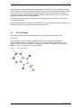
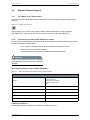
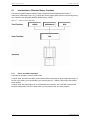
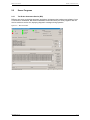
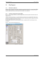
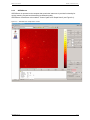
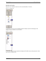
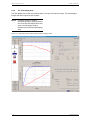
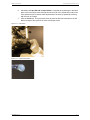
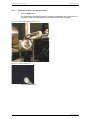
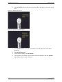
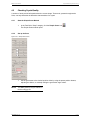
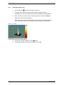
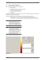
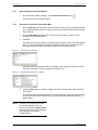
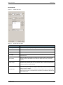
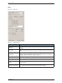
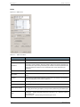
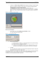
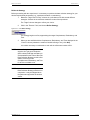
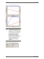
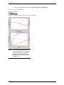
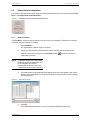
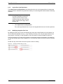
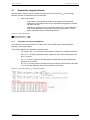
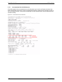
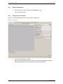
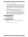
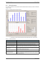
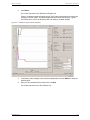
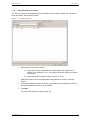
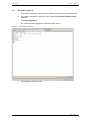
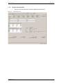
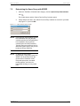
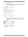
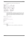
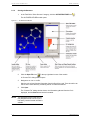
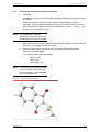
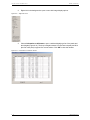
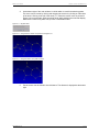
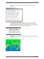
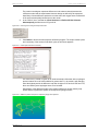
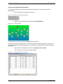
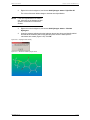
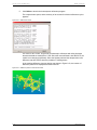
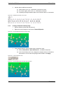
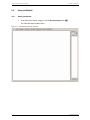
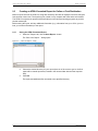
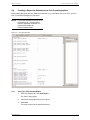
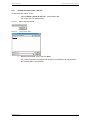
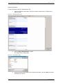
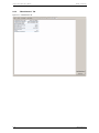
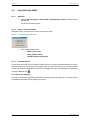
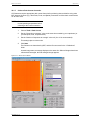
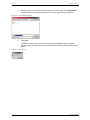
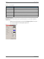
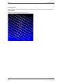
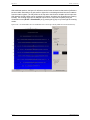
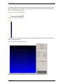
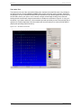
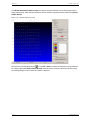
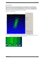
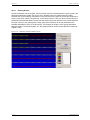
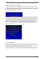
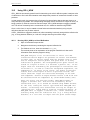
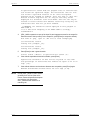
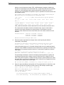
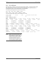
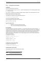
Structure Solution and Refinement
8.3.2
Labelling the Atoms
1.
NOTE:
APEX2 User Manual
Left-click the peaks for the two oxygen atoms to select them (Figure 8.14).
If it is difficult to see the color and
labels, change the color scheme with
Preferences > Background Color.
Choose colors and click Apply. Click
Cancel to exit the background color
mode.
Figure 8.14 —Model with probable oxygen peaks selected
2.
Right-click in the display, and choose Labelling... from the right-click menu.
The Atom Labelling box opens.
Figure 8.15 —Atom labelling box
3.
8 - 12
Label the selected atoms as oxygen. Do this in one of two ways:
•
Click the “Element” field and type the element symbol (case does not matter).
•
Click the El button to the right of the “Element” field to open a periodic table.
Click the appropriate element symbol to choose it (the periodic table will
automatically close).
DOC-M86-E02078
APEX2 User Manual
Structure Solution and Refinement
Figure 8.16 —Periodic table for choosing atom types
4.
Click Relabel to relabel and number the peaks sequentially in the order they were
selected, starting with the number in the “First Sequence #” field.
5.
To label the carbon atoms, select the remaining peaks in the order you want them
labeled.
6.
In the labelling tool, change the element type to C (carbon).
The starting atom number changes to 1 (i.e., the first available number for carbon
atoms).
8.3.3
7.
Click Relabel to relabel the carbon atoms.
8.
When all atoms are labeled and the molecule is ready for refinement, click Cancel.
Refining the Model
1.
In XSHELL’s Tool Icon Bar, click the Refine icon
> Refine.
, press [Ctrl]+[R], or choose Refine
The “Refine” window opens.
2.
Click Refine to launch XL (the least-squares refinement program) using the default
parameters as given in Figure 8.17.
Figure 8.17 —“Refine” menu
DOC-M86-E02078
8 - 13
Structure Solution and Refinement
APEX2 User Manual
After a few seconds, the “Refine” window opens containing output results for the
calculation.
Figure 8.18 —Isotropic refinement output
In the output displayed above, note that the R1 value is 0.09. This is typical for a
preliminary isotropic refinement for an organic molecule with data to a resolution of
0.75Å, and no hydrogen atoms included. The refinement program also indicates that the
model needs to be inverted to get the correct absolute structure.
NOTE:
This indication of the absolute
configuration is usually reliable, but all
assignments of absolute structure
should be confirmed later in the
refinement process by including TWIN
and BASF commands in the instruction
input.
3.
Click OK to return to XSHELL. The display refreshes with the results of the least-squares
calculations.
Figure 8.19 —Model after isotropic refinement
8 - 14
DOC-M86-E02078
APEX2 User Manual
Structure Solution and Refinement
The peaks in the diagram represent differences in the electron density between the
refinement model and the experimental electron density as defined by the measured
data. Many of these difference peaks are near the sulfur and oxygen atoms. Refinement
of all atoms anisotropically should improve the model.
4.
In the “Refine” menu, activate the Invert Structure and Refine All Non-H Atoms
Anisotropically checkboxes as in Figure 9.24.
Figure 8.20 —Inverting and choosing anisotropic refinement
5.
Click Refine to launch the least-squares refinement program. The output window opens
and a summary of the results of individual cycles of refinement appears.
Figure 8.21 —Least-squares refinement summary
The value for R1, 0.0459, is typical for an initial anisotropic refinement with no hydrogen
atoms included. Since the mean shift/esd is greater than 0.1, the model is still changing.
Since the highest peak in the difference map has a height of 0.47 and is 0.97Å from C10,
there are certainly some hydrogen atoms to be included.
Examination of the difference peaks in the resulting difference electron density map
shows that the top difference peaks all correspond to hydrogen atoms.
Figure 8.22 —Difference peaks correspond to expected hydrogen atom positions
DOC-M86-E02078
8 - 15
Structure Solution and Refinement
APEX2 User Manual
Viewing Atomic Displacement Parameters
It is generally good practice to examine the displacement parameters at this point in structure
determination.
1.
Remove difference peaks with the slider tool.
Figure 8.23 —Removing all Q peaks with the slider bar
2.
Right-click in the background, and choose Thermal Ellipsoids.
Figure 8.24 —Thermal ellipsoid plot
Generating a List of Equivalent Isotropic Displacement Parameters
In addition to the thermal ellipsoid plot, a list of Ueqs (equivalent isotropic displacement parameters)
can be generated by requesting information on all of the atoms. Examining these values for outliers is
good practice.
1.
Right-click in the background, and choose Information on All Atoms.
The “Information on All Atoms” window appears.
Figure 8.25 —List of parameters with Ueq to the right
8 - 16
DOC-M86-E02078
APEX2 User Manual
2.
Structure Solution and Refinement
Sort the atoms.
Reasonable Ueq Values
For the ylid molecule, the Ueq values are reasonable if there are:
•
lower values for the sulfur atom and the five-member ring;
•
higher values for the terminal atoms — methyls and carbonyls; and
•
sensible numbers for the six-member ring — lower for C8 and C9, higher for C5 and C6,
and in between for C4 and C7.
Sorting Atoms
When examining the values in the “Information on All Atoms” window is difficult because the atoms are
not in order, the atoms may be sorted.
1.
Right-click on the window’s background, and choose Sort… to sort the atoms into a
sensible order.
An Atom List box appears to the right of the molecule display. Since S1, O1 and O2 are
in a reasonable order, only the carbon atoms need to be ordered.
Figure 8.26 —Selecting carbons for sorting
NOTE:
Generally, it is easier to sort and
number atoms before adding hydrogen
atoms.
2.
Select the atoms to be sorted (i.e., click and drag over the atoms) and move them to the
Sort Bin (i.e., click Move Selected Atoms to Sort Bin).
Figure 8.27 —carbon atoms in Sort Bin
DOC-M86-E02078
8 - 17
Structure Solution and Refinement
3.
After the atoms are in the Sort Bin, click Sort (Alpha-Numeric).
4.
Select “O2”, and click Insert All After as in .
APEX2 User Manual
Figure 8.28 —Sorted atoms with the “insert after” atom (i.e., O2) selected
5.
Click OK to accept the sorting.
Adding Hydrogen Atoms
After refining the non-H-atoms, refine the hydrogen atoms either by:
•
renaming the Q-peaks using the Labelling tool, and then including them in the
refinement; or
•
including the hydrogen atoms in fixed idealized positions, riding on the atoms to which
they are attached.
In this example, we illustrate the latter fixed idealized method.
NOTE:
In some cases (e.g., hydrogen atoms
on hetero atoms or on geometrically
strained carbon atoms), it is better to
refine the hydrogen atom positions. A
general rule is to refine if there is some
doubt about the position of the
hydrogen atom and there is difference
electron density present.
1.
Use the slider tool to remove all of the Q peaks.
Figure 8.29 —Refined model with difference peaks removed
8 - 18
DOC-M86-E02078
APEX2 User Manual
2.
Structure Solution and Refinement
Right-click on the background, and choose Add Hydrogen atoms > Hybridize All.
The colors of the atom labels change to indicate atom hybridization.
NOTE:
If the atom hybridizations are hard to
see, right-click on the background and
open the “Information on All Atoms”
window.
3.
Right-click on the background, and choose Add Hydrogen atoms > Calculate
Hydrogens.
4.
A warning appears indicating that the hydrogen atoms have been provisionally added
and that the final addition with naming will take place when the least-squares
calculations are started (Figure 8.30). Click OK.
Figure 8.30 —Hydrogen atom warning
Figure 8.31 —Model with added hydrogen atoms
DOC-M86-E02078
8 - 19
Structure Solution and Refinement
5.
APEX2 User Manual
Click Refine to launch the least-squares refinement program.
The output window opens, and a summary of the results of individual refinement cycles
appears.
Figure 8.32 —Refinement results
The value for R1, 0.0281, is typical for an anisotropic refinement with riding hydrogen
atoms and a data set measured to 0.75Å. Since the mean shift/esd is less than 0.01, the
model is not changing significantly. Since the highest peak and the deepest hole in the
difference map are similar, there are probably no missing atoms.
In the resulting difference electron density map shown in Figure 8.33, the number of
difference peaks to be displayed has been left at 20.
Figure 8.33 —Difference peaks in a well-refined model
8 - 20
DOC-M86-E02078
APEX2 User Manual
8.3.4
NOTE:
Structure Solution and Refinement
Refining for Publication with XSHELL
1.
Obtain a view that is much easier to interpret by reducing the number of difference peaks
in the “Refine” menu (Figure 8.34).
2.
For the final cycles of refinement, reduce the number of peaks to be displayed to five and
turn on “Use Suggested Weights” and “Generate ACTA(CIF) Information File” as shown
in the next two figures.
If the suggested weights vary
significantly from 0.06 and 0.00, then
change the values to 0.06 and 0.00.
Figure 8.34 —Reduce the number of difference peaks
Figure 8.35 —Select weights and request ACTA output
Figure 8.36 shows a difference map with the number of peaks set at 5.
Figure 8.36 —Difference peaks
3.
Click the Edit File button, choose the .ins file, and click OK to open the instruction file for
XL. This allows you to add instructions that are not directly available in the GUI.
Figure 8.37 —“Edit File” window
DOC-M86-E02078
8 - 21
Structure Solution and Refinement
4.
APEX2 User Manual
Add the desired additional commands.
4.1. Check that the TEMP (i.e., temperature) command is correct.
4.2. For torsion angles, add a CONF (i.e., confirmation) command.
4.3. If planarity and angles between planes are of interest, add MPLA commands.
Figure 8.38 —Additional instructions in the .ins file
8.3.5
Creating a Publication-Quality Image
1.
Remove difference peaks with the slider tool.
2.
Right-click on the background, and choose Thermal Ellipsoids.
Figure 8.39 —Thermal ellipsoids with large hydrogen atoms
3.
If the hydrogen atoms in Figure 8.39are large, change their sizes:
3.1. Choose Preferences > Atom Preferences... in XSHELL’s Menu Bar.
3.2. In the “Atom Preferences” area, change the hydrogen radius to 0.08 and the
bond radius to 0.15 to make the hydrogen atoms smaller. Click Apply.
Figure 8.40 —“Atom Preferences” menu
Figure 8.41 —Thermal ellipsoid plot with smaller hydrogen atoms
8 - 22
DOC-M86-E02078
APEX2 User Manual
4.
Structure Solution and Refinement
Position atom labels by right-clicking on the atom and choosing Position Label.
Figure 8.42 —Positioned atom labels
5.
Convert this image into a high-quality .jpg file for inclusion into reports by choosing
Render > Color > To High Quality JPEG File.
NOTE:
A message may appear that the font
file needs to be defined: “Please set
your font directory for the first time for
opengl rendering.” If this happens,
choose Preferences > OpenGL
Preferences, and click on the
TrueType font For.OpenGL.
NOTE:
In Windows, browse to
C:\bn\xshell\fonts\
NOTE:
In Linux, navigate to
/usr/local/bin/xshell/fonts. Choose a
font.
Figure 8.43 —Final rendered thermal ellipsoid/atomic displacement parameter plot
DOC-M86-E02078
8 - 23
Structure Solution and Refinement
APEX2 User Manual
This page intentionally left blank.
8 - 24
DOC-M86-E02078
9
Using the Report Generation Module
9.1
Preparing for Report Generation
Before creating the report, make sure that your *.ins file has the correct values for the final structure:
NOTE:
•
Correct formula (SFAC and UNIT instructions)
•
Correct Z value (ZERR instruction)
•
Final cell constants with ESDs (from the final *_0m._ls file)
•
Correct atom sorting and labelling
•
TEMP instruction (in °C) (e.g., TEMP -173 for 100K)
•
SIZE instruction
•
ACTA instruction
•
BOND $H instruction
•
CONF instruction for torsion angles (if applicable)
•
HTAB instruction for hydrogen bonds (if applicable)
You may need to edit the instructions
file to add one or more of these
instructions or parameters. If so, click
Refine with XL to generate the .cif file
that you will import into the report.
Figure 9.1 — Instructions added to .ins file
DOC-M86-E02078
9-1
Using the Report Generation Module
9.2
Using the Module
9.2.1
Starting the Module
1.
In the Task Bar’s “Report” category, click the Generate Report icon
APEX2 User Manual
.
The Generate Report module opens.
Figure 9.2 — Generate Report module: initial view
9-2
DOC-M86-E02078
APEX2 User Manual
9.2.2
Using the Report Generation Module
Choosing a Template File
To set the formatting for your report, you will choose a template on which your report will be based.
Template files are contained in the directory C:/bn/src/report.
1.
In the right-hand section of the module, use the drop-down menu or the Browse button
to find the desired template file:
•
Choose apex2.zip to format the report as output from the module, without
instrument-specific text.
•
Choose x2s.zip to format the report with SMART X2S-specific text and data.
•
Choose acta.cif to format the report as a .cif file for submission to Acta
Crystallographica.
Figure 9.3 — Choosing a template file
2.
Click Open.
The module retrieves your project’s data and populates the report based on the selected
template.
Proceed to Section 9.3 for information on creating a report for online or print distribution.
Proceed to Section 9.4 for information on creating a report for submission to Acta Crystallographica.
DOC-M86-E02078
9-3
Using the Report Generation Module
9.3
APEX2 User Manual
Creating an HTML-Formatted Report for Online or Print Distribution
Bruker’s report format is an HTML file, along with necessary Java files to display the structure using the
free structure viewer Jmol. The report may be viewed on any computer with Java and a web browser.
The HTML file may also be opened in Microsoft Word or other word-processing programs to produce
printed manuscripts.
Before saving the report, add any additional information (e.g., information from your .cif file, your run
lists, your contact information) to the report.
9.3.1
Saving the HTML-Formatted Report
1.
Under the “Report” tab, click the Save Report... button.
The “Save Your Report...” dialog opens.
Figure 9.4 — “Save Your Report...” dialog
2.
Choose the desired directory for your report (there is no file name to type in; the final
report will be named report.html, located in the chosen folder with the other required
files).
3.
Click OK.
The report and additional files are saved to the specified directory.
9-4
DOC-M86-E02078
APEX2 User Manual
9.4
Using the Report Generation Module
Creating a Report for Submission to Acta Crystallographica
Before saving the report, add any additional information (e.g., information from your .cif file, your run
lists, your contact information) to the report.
NOTE:
If you need information from the .cif file
generated by XL, you will need to
import it regardless of whether you
have already created an
HTML-formatted report.
Figure 9.5 — CIF report initial view
9.4.1
Saving the CIF-Formatted Report
1.
Under the “Report” tab, click Save Report....
The “Save” dialog opens.
2.
Choose the desired directory for your report.
3.
Click Save.
The report is saved to the specified directory.
DOC-M86-E02078
9-5
Using the Report Generation Module
9.5
APEX2 User Manual
Adding Additional Information to the Report
To achieve a publication-quality report, you will need to add certain information to the report before
saving it. This information may include:
•
Information from the .cif file generated by XL (e.g., torsion angles, hydrogen bonds)
•
The experiment’s run list
•
Additional information (e.g., diffractometer information, name of institution, contact
information, etc.)
Figure 9.6 — Torsion and hydrogen bonds missing
9-6
DOC-M86-E02078
APEX2 User Manual
9.5.1
Using the Report Generation Module
Adding Information from a .CIF File
To add information from a .cif file:
1.
Choose Report > Import XL CIF File... from the Menu Bar.
The “Import CIF File” window opens.
Figure 9.7 — Report > Import XL CIF File...
Figure 9.8 — “Import CIF File” dialog
2.
Browse to the desired .cif file, and click Open.
The .cif file’s information is imported into the report. If information is already present in
the imported fields, it is overwritten.
DOC-M86-E02078
9-7
Using the Report Generation Module
9.5.2
APEX2 User Manual
Adding the Run List
To add the run list:
1.
Choose Report > Import Run List... from the Menu Bar.
A run list selection dialog appears.
Figure 9.9 — Report > Import Run List...
Figure 9.10 —“Select Runs” dialog
2.
Browse to your project’s location, choose the desired runs, and click OK.
The run list is imported into the report.
9-8
DOC-M86-E02078
APEX2 User Manual
9.5.3
Using the Report Generation Module
Adding Additional Information
To add additional information to the report, simply choose the desired tab (e.g., the “Miscellaneous”
tab), and edit the information directly in the necessary fields. When you return to the “Report” tab, the
new information will be updated in the report.
Importing and Exporting Additional Information
The “Miscellaneous” tab allows you to import and export report information (e.g., for generic information
that is reused often, such as experiment setup and contact information).
Importing Information
To import information into the “Miscellaneous” tab:
1.
Click the Import Items... button.
The “Import Items” dialog opens.
Figure 9.11 — “Import Items” dialog
2.
Browse to the .pcf file that contains the desired information.
3.
Click Open.
The information is imported into the report. If information is already present in the
imported fields, it is overwritten.
DOC-M86-E02078
9-9
Using the Report Generation Module
APEX2 User Manual
Exporting Information
To export information from the “Miscellaneous” tab:
1.
Click on the fields to select them. [Ctrl]-click to select multiple items, or [Shift]-click to
select a range.
Figure 9.12 —Selecting data for export
2.
Click the Export Selected Items... button.
The “Export Items” dialog opens.
Figure 9.13 —“Export Items” dialog
3.
9 - 10
Choose a directory and filename for the exported information, and click Save to save the
information as a .pcf file.
DOC-M86-E02078
APEX2 User Manual
9.6
Using the Report Generation Module
Report Sections
The module displays the report in a series of tabbed sections for review before saving.
9.6.1
“Report” Tab
The Report tab gives an at-a-glance view of the report as it will appear after saving (either as HTML or
as a .cif file). It contains all of the sections that are shown in the other tabs.
Figure 9.14 —“Report” tab
DOC-M86-E02078
9 - 11
Using the Report Generation Module
9.6.2
APEX2 User Manual
“Atoms” Tab
The “Atoms” tab lists the atoms in the solved structure by type. The columns are sortable.
Figure 9.15 —“Atoms” tab
9 - 12
DOC-M86-E02078
APEX2 User Manual
9.6.3
Using the Report Generation Module
“Bond Lengths” Tab
Bond lengths and ESDs for the structure are given in this tab. The columns are sortable. Additionally,
you can move an individual entry in the table up or down by selecting it with the mouse and clicking the
and
buttons in the lower right-hand corner.
Figure 9.16 —“Bond Lengths” tab
DOC-M86-E02078
9 - 13
Using the Report Generation Module
9.6.4
APEX2 User Manual
Bond Angles
Bond angles and ESDs are given in this tab. The columns are sortable. Additionally, you can move an
individual entry in the table up or down by selecting it with the mouse and clicking the
and
buttons in the lower right-hand corner.
Figure 9.17 —“Bond Angles” tab
9 - 14
DOC-M86-E02078
APEX2 User Manual
9.6.5
Using the Report Generation Module
“Torsion Angles” Tab
Figure 9.18 —“Torsion Angles” tab
DOC-M86-E02078
9 - 15
Using the Report Generation Module
9.6.6
APEX2 User Manual
“Miscellaneous” Tab
Figure 9.19 —“Miscellaneous” tab
9 - 16
DOC-M86-E02078
10 Appendices
DOC-M86-E02078
10 - 1
Appendices
APEX2 User Manual
10.1
Using BCP with APEX2
10.1.1
Start BCP
1.
Choose Start > Programs > Bruker AXS > Administration > BCP, or double-click the
desktop icon.
The BCP main window opens.
10.1.2
Select a Connection Mode
When BCP starts, it prompts you to choose a connection mode.
Figure 10.1 —“Select connection mode” window
1.
10.1.3
Click the appropriate button:
•
Master (full control)
•
Slave (monitor status)
•
No BIS (off-line/configuration)
Parameter Menus
The left-hand pane of BCP’s main window contains menus for various instrument parameters. Most of
these parameters will never have to be changed by the user, but some values (e.g., the detector beam
center) may need to be updated from time to time. If changes are made, the parameters are updated by
clicking the Save button
.
The "Instrument" Category
This menu contains the configuration parameters for the goniometer and generator. These are set prior
to installation and should not be changed by the user.
10 - 2
DOC-M86-E02078
APEX2 User Manual
Appendices
The "Generator" Category
If the software has control over the generator, this menu contains the power settings and limits for the
generator. Otherwise, most of these parameters are accessible from the generator’s I/O panel.
•
The “Tube Limits” area contains the generator’s power limit parameters. These values
are set up prior to or during installation and should not need to be changed.
•
The “Preferred” area contains the values for the standard user settings. If “user settings”
are selected when setting the generator power in BCP, the generator will ramp up to the
preferred values. The warm-up delay is the time delay between when the generator
ramps up to the user settings and when the first image can be taken. The default should
be 120 seconds (00:02:00 hr:min:sec).
•
The “Standby” area contains target parameters for the generator if it is idle for the
prescribed time. The default power settings are 45 kV and 5 mA. The bias can remain at
the optimum setting. If desired, the idle time counter can be disabled during weekday
hours.
Some users may want to disable the “Standby” feature. To do this, set the idle time to 3
days (72 hours) or longer, and the activate the Exclude weekday checkbox.
10.1.4
Change the Detector’s Beam Center
1.
Under the “Detector” category in BCP’s left-hand pane, click Settings.
The detector settings information appears.
Figure 10.2 —Detector settings
DOC-M86-E02078
10 - 3
Appendices
APEX2 User Manual
2.
In the “Detector center at default frame size” area, right-click on any of the values and
choose Modify.
The “Enter detector center parameters” window opens.
Figure 10.3 —“Enter detector center parameters” window
3.
Enter the desired values for Xraw and Yraw. Click OK.
4.
If you have a detector that requires a spatial correction, click the Raw => Unw button.
If this button is disabled (i.e., grayed-out), load the spatial correction table under Tools >
Spatial and try again.
5.
10 - 4
Save the changes by choosing File > Save.
DOC-M86-E02078
APEX2 User Manual
10.1.5
Appendices
Collect a Dark Current Correction
CCD detectors require appropriate dark current frames before collecting data, and before using other
BCP detector functions (e.g., Bad Pixels, Flood, and Spatial). Remember to collect dark current frames
for all frame sizes.
NOTE:
Be sure that the detector is cooled to its
normal operating temperature before
collecting a dark current correction.
1.
Choose Tools > Dark Current.
2.
Set the “Seconds per exposure” value to the same time needed by your experiment (or
your bad pixel, flood, or spatial frame).
3.
Set the “Number of exposures to average” value to 9 (9 to 16 is recommended).
This setting helps to reduce noise.
4.
Click Start.
The filenames are determined by BCP, and the files are stored in the “/Calibrations”
folder.
As each image starts, a message displays on the status line. When all images have been
collected and averaged, the final averaged image appears.
Figure 10.4 —Dark current collected
DOC-M86-E02078
10 - 5
Appendices
10.2
APEX2 User Manual
Set Default Orientation Matrix Scans in the bn-config.py File
The bn-config.py file contains default orientation matrix run settings.
1.
Open the bn-config.py file in a text editor.
2.
Edit the following parameters (or, if they are not present, add them at the end of the file):
2.1. Set the 2theta angle using the parameter
perpendicular_matrix_runs_2theta.
2.2. Set the detector distance using the parameter
perpendicular_matrix_runs_distance.
2.3. Set the extent of the scan using the parameter
perpendicular_matrix_runs_sweep.
For example, a value of 3 for this variable would mean that six 0.5° images
would be collected for a total of 3°.
2.4. Set the number of scans to collect using the parameter
perpendicular_matrix_runs_nr_sweeps.
If more than one scan is requested, the program uses different settings of the
phi axis for each scan.
2.5. Set the default exposure time using the parameter
perpendicular_matrix_runs_frametime.
3.
NOTE:
10 - 6
Save the bn-config.py file, and exit the text editor.
If APEX2 is running when the
bn-config.py file is updated, it should
be restarted so that it reads the
updated bn-config.py file.
DOC-M86-E02078
APEX2 User Manual
10.3
Appendices
Face Indexing with the Crystal Faces Module
In order to perform numerical correction for intensity data, the crystal’s faces must be indexed. This
allows a very exact crystallographic description of the crystal’s shape.
Once you have a unit cell for your crystal, the Face Indexing module allows you to define faces directly
over images of the crystal. As you define more and more faces, The module automatically determines
the dimensions of the crystal.
This example uses a large crystal for which the unit cell has already been determined.
10.3.1
Starting the Crystal Faces Module
1.
From the Task Bar’s “Scale” category, click the Crystal Faces icon
.
The Crystal Faces module starts.
10.3.2
Collecting a Video Zip Stream
To index the faces, first collect a video zip stream, which is a series of images taken with the video
microscope as the crystal is rotated through 360° about the phi axis.
NOTE:
For the best results, make sure that
lighting conditions are optimal for the
crystal you are viewing. If possible, try
to illuminate the crystal for optimum
contrast between the crystal and the
background. Also, it may desirable to
use multiple light sources to illuminate
several faces simultaneously.
1.
If no video zip stream has been collected for this crystal, a dialog appears prompting you
to acquire a new video zip stream or load an existing one.
Figure 10.5 —“Video Source” window
DOC-M86-E02078
10 - 7
Appendices
APEX2 User Manual
2.
Because we have not yet taken a video zip stream for this crystal, click Acquire New....
The “Save Video File” dialog (defaulted to your current project directory) appears.
Figure 10.6 —“Save Video File” dialog
3.
Click Save.
If VIDEO is not open, it will open with a progress bar showing the video zip stream
collection. When the video zip stream is fully collected, the Face Indexing initial view will
appear.
Figure 10.7 —Progress bar
10 - 8
DOC-M86-E02078
APEX2 User Manual
10.3.3
Appendices
The Crystal Faces Module Interface
The Face Indexing module uses a dial at the bottom of the screen to step through the images of the
crystal, and a tool called the T-tool to define faces. The Face List, shown on the right, displays the faces
you have defined for the crystal and their distance from the instrument center.
Figure 10.8 —Crystal Faces module: initial view
Table 10.1 — Face indexing controls
Item
Description
Show T-tool
Show and hide the T-tool for a better view of the crystal faces.
Max. Miller index:
The highest Miller index shown as face normals in the overlay.
Max. out-of-plane angle
(deg):
When the T-tool snaps to a face normal, the plane you define may differ from the specified
index by a maximum of this amount.
Show possible face normals
The module suggests face normals.
Snap to possible face
normals
The T-tool snaps to the suggested face normals.
Dial (or mouse wheel)
Use the dial to rotate around 360° of phi. The right-click menu lets you rotate phi by 180° to
define parallel faces.
Crystal face information
Shows the Miller indices of a given face, the face’s distance from the instrument center, and
the out-of-plane angle.
DOC-M86-E02078
10 - 9
Appendices
APEX2 User Manual
Table 10.2 — Face list controls
Item
Description
Unit Cell
Displays the unit cell that the module uses to display faces in the overlay.
H,K,L
Miller indices of the normal to the specified face.
Distance (mm)
The specified face’s distance to the center of the instrument.
Remove Invisible Faces
Faces obscured by the body of the crystal are removed from the Face list.
Closed:
Displays whether the faces you have defined encapsulate a closed volume.
Size (mm):
Dimensions of the crystal, calculated according to the defined faces.
Setting View Options
Depending on the color and reflectivity of the crystal and background, you may want to adjust the
display colors.
1.
Right-click in the image display area, and choose Configure Overlay from the menu.
The “Overlay Configuration” window appears (Figure 10.9).
Figure 10.9 —“Overlay Configuration” window
10 - 10
DOC-M86-E02078
APEX2 User Manual
10.3.4
Appendices
Specifying Crystal Faces
1.
Use the dial control at the bottom of the screen (or use the mouse wheel) to rotate the
crystal until one of the faces is parallel to the microscope axis as in Figure 10.10.
Note that, because Show T-Tool and Show possible face normals are activated, the
module suggests possible faces (whose indices are within the Max. Miller Index
parameter) with dotted lines.
Figure 10.10 —Face parallel to microscope axis
2.
Move the mouse cursor to the dotted line that is perpendicular to the face.
The mouse cursor snaps to the possible face normal. A line appears to show the
possible face. This line defines a plane along the microscope axis, which should be
parallel to the crystal face.
3.
Use the mouse to move the line until it touches the crystal face.
Figure 10.11 —Face normals
DOC-M86-E02078
10 - 11
Appendices
APEX2 User Manual
4.
Click to fix the face.
An entry appears in the Face List showing the Miller Indices of the crystal face, along
with the face’s distance from the instrument center.
Figure 10.12 —Fixing the face
5.
Repeat the steps in this Section to specify all of the crystal’s visible faces.
If the module does not suggest a face normal for a certain face, you can increase the
value in the “Max. Miller index” field to show more suggested normals. As you define
more faces, the module will begin to display its geometric model of the crystal,
superimposed over the video images (Figure 10.13).
Figure 10.13 —Some—but not all—faces defined
Figure 10.14 —All faces defined
10 - 12
DOC-M86-E02078
APEX2 User Manual
10.3.5
Appendices
Editing the Face List
Consider Figure 10.15. The face (1 3 -2) does not appear to define a face correctly. Removing this face
will give a more accurate model of the crystal.
Figure 10.15 —Face (1 3 -2) is incorrect
1.
In the Face List, select the HKL (1 3 -2).
2.
Right-click and choose Remove. The face is removed from the list and the model is
improved (Figure 10.17).
DOC-M86-E02078
10 - 13
Appendices
NOTE:
APEX2 User Manual
Alternatively, you can select Clear List
to start over, or Add and Edit to define
your own faces and see where they
appear on the crystal.
Figure 10.16 —Face List right-click menu
Figure 10.17 —Face (1 3 -2) removed
10.3.6
10 - 14
Scaling with Face Indices
1.
When all faces are defined, the module has accurate crystal dimensions (as shown in
the bottom right-hand corner). At this point, you can exit the Face Indexing module and
proceed with scaling.
2.
In the Scale module, be sure to select Numerical Absorption Correction under the
“Setup” tab.
DOC-M86-E02078
APEX2 User Manual
10.4
Appendices
The Reciprocal Lattice Viewer Module
The Reciprocal Lattice Viewer module is a very powerful tool for viewing the harvested reflections in a
reciprocal lattice.
10.4.1
Start the Reciprocal Lattice Viewer Module
1.
In the Task Bar’s “Evaluate” section, click the Reciprocal Lattice Viewer icon
.
The Reciprocal Lattice Viewer module opens.
The module automatically reads the reflections from the current project and displays
them as a reciprocal space plot.
10.4.2
Views and Tools
Figure 10.18 is a typical unoriented view after import. The gray circles are more intense reflections, i.e.,
those with higher I/sigma(I). The black dots represent less intense reflections. The intensity key slider at
the bottom of the window can be used to change the selection criterion.
Figure 10.18 —Unoriented view
DOC-M86-E02078
10 - 15
Appendices
APEX2 User Manual
Other tools can be accessed by right-clicking on the background to give the “Quick Tools” menu (Figure
10.19), and by choosing RLATT in the Menu Bar (Figure 10.20).
Figure 10.19 —Quick Tools menu
Figure 10.20 —Full menu tools
Additional context-sensitive information is available by clicking the “What’s This” help arrow in the Menu
Bar.
Figure 10.21 —“What’s This?” help icon
10 - 16
DOC-M86-E02078
APEX2 User Manual
Appendices
For example, clicking the “What’s This?” help icon and then clicking in the work area (i.e., the gray area
to the right of the lattice display) gives the shortcuts shown in Figure 10.22. Clicking on the blue
background gives the hints shown in Figure 10.23.
Figure 10.22 —Shortcut keys and commands
Figure 10.23 —3D display information window
DOC-M86-E02078
10 - 17
Appendices
APEX2 User Manual
Orienting Views
Move the mouse to rotate the lattice display. It is possible to easily see rows and non-fitting peaks (see
Figure 10.24).
Figure 10.24 —Display looking down layers of reflections
10 - 18
DOC-M86-E02078
APEX2 User Manual
Appendices
By moving the intensity slider at the bottom of the display, it is easy to deselect weak reflections. In
Figure 10.25, the reflections between the layer lines all turn black when the intensity filter is moved to
the left.
Figure 10.25 —Display looking down layers of reflections. Weaker reflections, i.e., those with smaller I/sigma(I), are black because
the “Intensity Filter” slider has been moved to the left.
DOC-M86-E02078
10 - 19
Appendices
APEX2 User Manual
With additional rotations, the layers of reflections can be further oriented so that stacks of reflections
become visible. Sometimes it is quite useful to right-click on the background and choose Z-rotations
from the rotation options. The 2D profiles on the top and to the left are a valuable aid in this process.
With practice, the 2D profiles can be organized into clusters. As shown, the 2D profiles are counting
intensity. The counting mode can be changed to spot count or turned off completely using the
Visualization menu (RLATT > Visualization) or by pressing the [s] key to cycle through the counting
modes.
Figure 10.26 —An oriented lattice view. The Visualization menu is to the right. The 2D profiles are to the left and to the top.
10 - 20
DOC-M86-E02078
APEX2 User Manual
Appendices
The distance between layers can be measured by clicking on one of the clusters of lines in the 2D view
and then dragging to the next cluster. If you drag over three clusters, then the distance as measured
would need to be multiplied by three.
Figure 10.27 —Horizontal measured distance
Figure 10.28 —Vertical measured distance
The Orientation menu allows easy orientation if the cell is indexed. Press the [F1], [F2], or [F3] key or
click the appropriate button.
Figure 10.29 —Orientation menu with aligned view
DOC-M86-E02078
10 - 21
Appendices
APEX2 User Manual
The Lattice Tool
The Lattice tool is one of the most useful editing tools. Activate it from the Edit menu or by clicking on
the background and choosing Select > Lattice. When initially activated, nothing appears. Hold down
the [Alt] key to lock on a centroid and then left-click and hold on a spot. Now drag the mouse and line up
the line that is tied to your spot on a row. Choose a longer row and align carefully. Now, while still
holding the left mouse button, drag the second line to another row as shown in Figure A.13. Let go of
the button. If you want to start over, click on another spot and repeat the process. Using the [Alt] key is
optional, but it makes alignment of the lines easier and more accurate (Linux users may find that the
[Alt] key has operating system functions).
Figure 10.30 —Two lattice lines selected
10 - 22
DOC-M86-E02078
APEX2 User Manual
Appendices
Press the [+] key to add lines between the two you have marked. Press the [-] key to remove lines.
Figure 10.31 —View with most of the lattice lines selected (lines to the top and bottom are not selected).
DOC-M86-E02078
10 - 23
Appendices
APEX2 User Manual
Use the [Page Up] key to add lines to the outside of the previously selected lines (in this example, the
top and bottom). [Page Down] removes lines from the outside. Now all visible lines are selected. Note
that the selected reflections are turquoise.
Figure 10.32 —A view with all the layers selected
10 - 24
DOC-M86-E02078
APEX2 User Manual
Appendices
Click Invert Selection (in the “Editing Menu” (RLATT > Edit) under “Selection Helpers”). All of the
spots that do not touch the layer lines are now selected.
Figure 10.33 —Spots selected between layers
DOC-M86-E02078
10 - 25
Appendices
APEX2 User Manual
Click Delete Selected (finalized at save) to mark the selected reflections to be deleted (and turned
black). Alternatively, these selected reflections can be added to a group and then hidden using Select
Visible Groups.
Figure 10.34 —Selected reflections are black
Save the file by clicking the disk icon
, or use File > Save to remove the reflection from the reflection
list. Hiding a group with Select Visible Groups does not remove it from the reflection list. Either way,
the resulting image is much cleaner and easier to interpret.
10 - 26
DOC-M86-E02078
APEX2 User Manual
Appendices
The Unit Cell Tool
Enable the Unit Cell tool to put a colored box in the view. This allows you to see if reflections are
actually falling on the corners of the box (see Figure 10.35 and Figure 10.36). There are multiple
options in the Unit Cell tool. Select a Visible Plane displays individual planes. Select Plane Size
determines the boundaries of the planes and the number of unit cells displayed. Grid Planes mode
displays planes as grids with spacings determined by the lattice.
Figure 10.35 —Unit Cell tool enabled
Figure 10.36 —A view that zooms in on the Unit Cell tool. Almost all spots lie on the lines and planes defined by the unit cell. To
the left and right are two weaker reflections (black dots) that do not fit.
DOC-M86-E02078
10 - 27
Appendices
10.4.3
APEX2 User Manual
Defining Groups
Selected reflections can be grouped. This tool is most useful for examining twinned, split, ingrown, and
otherwise problematic crystals. For Figure 10.37, alternate rows were selected with the Lattice
Selection tool. In the Grouping Tools section of the tool boxes to the right, the current group was set to
Group 1 (red). Click “Add to Current Group” to turn these rows red. Then, the other rows and Group 13
(white) were selected and added. The box tool was used to select the reflection to the top left and these
were put in Group 3, the yellow group. Finally, some of the reflections to the top and bottom were
selected and added to Group 5, the blue group. This example of using the color groups generates a
flag-type display. For twinned crystals, etc., the groups would be used to denote different components
(Figure 10.38).
Figure 10.37 —Reflections selected for different groups
10 - 28
DOC-M86-E02078
APEX2 User Manual
Appendices
Figure 10.38 — A more practical use of the selection and color groupings. The two components of a rotational twin are colored yellow and red.
DOC-M86-E02078
10 - 29
Appendices
10.4.4
APEX2 User Manual
Measuring Distances and Angles
Right-click on the background and choose Measure to get tools for measuring distances and angles.
The Measure Distance tool gives two lines, much like the lines in the Lattice Selection tool, that can be
oriented and dragged to get lattice spacings (Figure 10.39). Use the [Alt] key to lock on spot centers for
easier orientation and more accurate measuring.
Figure 10.39 —Measure distance tool
With the Measure Angle tool, left-click, hold, and drag a line on a lattice layer ending on the spot that
will become the vertex of the angle. When the mouse is released, that point becomes the pivot point for
a new line. Moving the mouse with no buttons depressed gives angle measurements (Figure 10.40). As
described, the angle measurements will be done in 2D mode (i.e., the angle between the two lines
displayed). To measure an angle in 3D mode, hold the [Alt] key while selecting spots as above. The tool
will then lock on to spot centroids and the angle will be calculated using spot coordinates. This
eliminates errors that might result from measuring using the 2D projection of the current orientation.
Figure 10.40 —Measure angle tool
10.4.5
Writing a .p4p File
At the bottom of the Edit menu, there is a button for exporting all visible reflections to a .p4p file. The
.p4p file is a text file of crystal, instrument, and reflection information. If the cell and crystal orientation is
known, that information is included also (otherwise, dummy values are included).
The sequence of cleaning up a set of reflections using the Reciprocal Lattice Viewer module and then
exporting the results for input to CELL_NOW is a useful tool for dealing with hard-to-index crystals.
10 - 30
DOC-M86-E02078
APEX2 User Manual
10.5
Appendices
Using CELL_NOW
CELL_NOW is an extremely powerful tool for determining unit cells for difficult crystals. It analyzes a list
of reflections to find a cell and orientation matrix despite the presence of several twin domains or other
problems.
In initial search mode, the program tries to find sets of reciprocal lattice planes that pass close to as
many reflections as possible. The corresponding real space vectors are sorted on a figure of merit (1.0
being a perfect fit). After the vector list has been output, CELL_NOW attempts to suggest a suitable
cell. This will not necessarily be the conventional cell, so it should be checked using XPREP.
Once a cell is found, it may be rotated to locate further twin domains iteratively using only the
reflections that have not yet been indexed.
If CELL_NOW fails to suggest a sensible cell, either something is seriously wrong with the reflection list
(e.g., a wrong detector distance) or a cell axis is longer than the given search range.
10.5.1
Running CELL_NOW on a List of Reflections
1.
Open a Command Prompt window.
2.
Navigate to the directory containing the exported reflection list.
3.
For Windows or Linux, enter the command cell_now.
The terminal prints out an explanation of the program. Read this as it has useful
information about what the program is doing:
CELL_NOW analyses a list of reflections to find a cell and
orientation matrix despite the presence of several twin domains
or other junk. In initial search mode the program tries to find
sets of reciprocal lattice planes that pass close to as many
reflections as possible. The corresponding real space vectors are
sorted on a figure of merit (1.0 would be a perfect fit). In the
output these are followed by the percentages of reflections that
fit within 0.1, 0.2 and 0.3 times the interplanar separation, the
components a1, a2 and a3 of the vector, the angles to previous
vectors and a cross figure of merit to previous vectors. The
latter should be larger for reflections belonging to the same
twin component. Cosines of angles between vectors a and b can also
be calculated from the components by (a1*b1+a2*b2+a3*b3)/(a*b).
After the vector list has been output, CELL_NOW attempts to
suggest a suitable cell. This will not necessarily be the
conventional cell, so it should be checked using XPREP (without
an .hkl file) taking the lattice type found with CELL_NOW into
account. If necessary this conventional cell may be reinput in
'specified cell' search mode to find the orientation matrix. If
CELL_NOW fails to suggest a sensible cell, either something is
seriously wrong with the reflection list (e.g. a wrong detector
distance) or a cell axis is longer than the given search range.
DOC-M86-E02078
10 - 31
Appendices
APEX2 User Manual
In specified cell search mode the program tries to find the best
cell within the specified ranges. The reflections that fit this
cell within a specified fraction of all ?hree interplanar
spacings may be flagged as indexed, and a new .p4p or .spin file
written in which they have the 'H' flag so that they can be
displayed in a different color with RLATT. Then the cell may be
rotated to locate further twin domains iteratively using only the
reflections that have not yet been indexed.
** WARNING: the exhaustive search employed in this program is
VERY SLOW **
** so a CPU clock frequency of AT LEAST 3GHz is strongly
recommended **
4.
CELL_NOW requests the name of the input file and suggests a name for the output file.
Enter the name of the input file (For the output file, press [Enter] to accept the default).
Full name of .p4p, .spin or .drx file to read: example.p4p
999 reflections read in
Listing file [example._cn]:
514 reflections read in
Listing file [example._cn]:
5.
Press [Enter] to start a general search.
Initial search (<Enter>) or specified cell search (S):
6.
If the default superlattice threshold is suitable, press [Enter].
Superlattice threshold: an axis will be rejected if less than
this percentage of reflections has indices not equal to 2n or 3n
resp. [10]:
7.
If the default minimum and maximum distances are acceptable, press [Enter] again.
Minimum and maximum allowed values for cell edge [5 40]:
NOTE:
10 - 32
Usually CELL_NOW is used to search
generally for a cell, but if the cell is
known, choose the specified cell option
and enter the cell dimensions.
CELL_NOW will then search for a
matching cell.
DOC-M86-E02078
APEX2 User Manual
Appendices
After some period of time, a list of real space vectors sorted on a figure of merit (1.0
being a perfect fit) will be output. These are followed by the percentages of reflections
that fit within 0.1, 0.2 and 0.3 times the interplanar separation, the components a1, a2
and a3 of the vector, the angles to previous vectors and a cross figure of merit to
previous vectors. The latter should be larger for reflections belonging to the same twin
component. Cosines of angles between vectors a and b can also be calculated from the
components by (a1*b1+a2*b2+a3*b3)/(a*b).
Length, fom, #hits, %(0.1), %(0.2), %(0.3), components
Followed by angle/correlation to previous vectors:
12.692
0.902
30
94.493
99.999
99.999
-0.475
5.493
-11.432
11.016
90.0
0.798
0.891
20
99.098
99.698
99.899
0.491
-9.912
-4.782
16.802 0.836
139.0 131.0
0.754 0.755
24
93.793
99.398
99.698
-0.011
4.417
16.211
16.805 0.819
139.1 49.1 81.9
0.749 0.739 0.688
25
90.189
99.498
99.899
0.953
-15.402
6.654
80.379
93.692
98.898
-0.446
1.111
-27.668
27.701 0.736
43
78.477
156.6 66.6 64.4 17.5 133.2
0.687 0.659 0.620 0.645 0.569
92.091
97.296
1.396
-20.915
18.109
25.428 0.722
45
77.376 98.497
119.9 150.1 19.1 101.0 143.3 83.5
0.651 0.674 0.638 0.600 0.557 0.533
99.598
-0.496
14.332
20.999
18.381 0.688
35
72.271 86.285 91.791
89.3 127.1 67.3 113.8 103.2 104.5 58.9
0.596 0.605 0.556 0.544 0.480 0.484 0.487
-15.128
9.256
4.827
6.329 0.686
4
65.465 65.465 65.465
179.9 90.1 40.9 41.0 156.7 23.5 60.0 90.7
0.574 0.573 0.532 0.524 0.459 0.469 0.465 0.426
0.248
-2.729
5.705
14.648 0.684
18
73.873 85.484 91.090 -14.633
89.1 90.3 90.5 90.9 89.3 90.9 90.2 36.8 91.1
0.591 0.603 0.556 0.539 0.475 0.477 0.490 0.539 0.424
-0.652
0.025
27.693 0.741
19
23.4 66.6 162.4 115.7
0.675 0.657 0.638 0.616
.
.
.
---------------------------------------------------------------------------
DOC-M86-E02078
10 - 33
Appendices
APEX2 User Manual
After the vector list has been output, CELL_NOW attempts to suggest a suitable cell.
This will not necessarily be the conventional cell, so it should be checked using XPREP
(without an .hkl file) taking the lattice type found with CELL_NOW into account. If
necessary, this conventional cell may then be input in 'specified cell' search mode to find
the orientation matrix.
The following cells would appear to be plausible, but should be checked using XP
REP because they are not necessarily the conventional cells.
FOM, % with i
n 0 .2, a..gamma, volume and lattice type for potential
unit-cells:
1
1 .000
85.3
12.692 11.016 14.648
89.70
90.95
90.00
2047.7 P
-----------------------------------------------------------------------------Cell for domain 1:
12.692
11.016
14.648
89.70
90.95
90.00
Figure of merit: 0.619
%(0.1): 68.3
%(0.2): 85.3
%(0.3): 91.0
CELL_NOW has identified a domain that fits 85.3% of the data with a tolerance of 0.2.
The output shows a suitable cell with its orientation matrix, figure of merit and the
deviations of the input reflections from integer indices. This deviation is used to
determine which reflections fit this cell and which are left for further searches for new
domains.
Orientation matrix:
0.00164338 -0.00357404 -0.06816319
-0.03417112 0.08170117 -0.00385047
0.07098872 0.03940338 0.00098036
Maximum deviation from integer index [0.25]:
8.
Enter the maximum deviation from integer index cutoff (Typically the default is
reasonable). Press [Enter].
Percentages of reflections in this domain not consistent with lattice types:
A: 50.1, B: 49.9, C: 45.0, I: 48.9, F: 72.5, O: 64.3 and R: 65.8%
Lattice information (given as % of relevant reflections that do not fit a particular lattice)
should be used in XPREP to determine the conventional cell. Typically, for a lattice to be
present the % inconsistent should be less than 10, but problem crystals can make the
value higher.
Percentages of reflections in this domain that do not have:
h=2n: 36.3, k=2n: 49.8, l=2n: 49.3, h=3n: 69.1, k=3n: 67.2,
l=3n: 66.4%
This percentage information is useful for identifying supercell problems. Typically, the
percentages should be 30% or higher for the 2n values and 50% or higher for the 3n
values, but problem crystals or crystals with heavy atoms in special positions can make
the values lower. Low values for a particular class of reflections can suggest that an axis
is double (2n) or triple (3n) its correct length.
New cell from list (number), reorientate (R), accept (A) or quit (Q) [A]: A
9.
Enter A or just press [Enter] to accept this cell. The program asks for a name for a .p4p
file. Enter the name of the .p4p file for this solution (in this example, domain1.p4p).
.p4p or .spin file to write domain to:domain1.p4p
RLATT color-coding employed in file: domain1.p4p
White: indexed for first domain
Red: not yet indexed
877 reflections within 0.250 of an integer index assigned to domain 1,
877 of them exclusively;
122 reflections not yet assigned to a domain
10 - 34
DOC-M86-E02078
APEX2 User Manual
Appendices
10. 122 reflections, approximately 1/10 of the data, have not yet been indexed (assigned to a
domain). This is more than might be expected for random noise peaks. A search for an
additional domain makes sense. The domain 1 cell will be rotated to locate further twin
domains iteratively using only the reflections that have not yet been indexed. Enter S to
search for another orientation of the newly chosen cell.
Re-refine initial cell (R), search for next domain (S), quit (Q) or choosenew cell
from list (enter number) [S]: S
Cell for domain
2:
12.692
Figure of merit: 0.643
Orientation matrix:
11.016
%(0.1):
69.7
14.648
%(0.2):
89.70
97.5
90.95
%(0.3):
90.00
98.4
0.00598966 0.00402327 0.06807401
-0.03367313 -0.08180340 0.00480114
0.07099302 -0.03914713 -0.00221035
Rotated from first domain by 179.7 degrees about
reciprocal axis 1.000 0.001 -0.032 and real axis
Twin law to convert hkl from first to
this domain (SHELXL TWIN matrix):
0.999
0.003
-0.064
1.000
0.004
-1.000
0.006
0.002 -0.010
-0.019
-0.004
-0.999
CELL_NOW has identified an additional domain that fits 97.5% of the data with a
tolerance of 0.2. The relationship between this domain and the first domain and the
SHELXL TWIN matrix are reported. This example is for a rotational twin about the a*
axis.
The output shows a suitable cell with its orientation matrix, figure of merit and the
deviations of the input reflections from integer indices. This deviation is used to
determine which reflections fit this cell and which are left for further searches for new
domains.
11. Enter the maximum deviation from integer index cutoff (typically, the default is
reasonable).
Maximum deviation from integer index [0.25]:
12. Enter the name of the .p4p file for this solution (in this example domain2.p4p).
.p4p or .spin file to write domain to:domain2.p4p
RLATT color-coding employed in file: domain2.p4p
White: indexed for first domain
Green: current domain (but not in a previous domain)
Red: not yet indexed
691 reflections within 0.250 of an integer index assigned to domain 2,
119 of them exclusively;
3 reflections not yet assigned to a domain
Re-refine initial cell (R), search for next domain (S), quit (Q) or choose
new cell from list (enter number) [Q]
13. Enter <q> to exit CELL_NOW.
C:\struc\guest\twin>
NOTE:
At this point CELL_NOW has indexed a
two-component twin. The orientation
matrices for the two components are in
the domain2.p4p file.
DOC-M86-E02078
10 - 35
Appendices
10.5.2
APEX2 User Manual
CELL_NOW Output
After processing, in addition to the terminal output and the example._cn listing file written to disk,
CELL_NOW writes two .p4p files, domain1.p4p and domain2.p4p. The second of these is a
multicomponent .p4p for a two-component twin. It is shown below.
The following entries appear twice (once for each domain):
CELL, ORT1, ORT2, ORT3, ZEROES, ADCOR
CELL2, ORT12, ORT22, ORT32, ZEROES2, ADCOR2
This will eventually trigger SAINT to treat this data set as a twin.
FILEID SAINT
V6.43A
4.00
06/19/03 09:36:24 mraa
SITEID RufM
Ruf
TITLE [RCpCrCl2.nTHF]n
CHEM
C40H58Cr2Cl4O2
CELL
12.6918
11.0161
14.6480
89.7011
90.9494
90.0010
2047.695
CELLSD
0.0025
0.0022
0.0029
0.0300
0.0300
0.0300
1.024
ORT1
0.001643376
-0.003574040
-0.068163186
ORT2
-0.034171116
0.081701167
-0.003850471
ORT3
0.070988722
0.039403379
0.000980361
ZEROS
0.0000000 0.3249754 -0.0041494
0.0000
0.0000
0.0000
ADCOR
2.9302
-0.0047
0.0003
-0.8959
0.0123
0.0937
CELL2
12.6918
11.0161
14.6480
89.7011
90.9494
90.0010
2047.695
CELLSD2
0.0025
0.0022
0.0029
0.0300
0.0300
0.0300
1.024
ORT12
0.005989663
0.004023272
0.068074010
ORT22
-0.033673126
-0.081803404
0.004801138
ORT32
0.070993021
-0.039147127
-0.002210349
ZEROS2 0.0000000 0.3249754 -0.0041494
0.0000
0.0000
0.0000
ADCOR2
2.9302
-0.0047
0.0003
-0.8959
0.0123
0.0937
SOURCE Mo
0.71073
0.70930
0.71359
2.00000
50.00
40.0
NOTE:
10 - 36
SAINT+ users should be aware that
APEX2 Version 2 can import .p4p files
created with CELL_NOW, and the
Integrate Images module will handle
the multiple orientation matrices
correctly. There is no longer a need to
use the standalone SAINT+ program.
DOC-M86-E02078
APEX2 User Manual
10.6
Appendices
Configuring the Suite
The Bruker Suite includes the ability to customize many features of the program. Most customizations
should be left to the site administrator, but some introduction is appropriate.
The following is a collection of examples of possible changes to the configuration files that control the
look and feel of the GUI.
10.6.1
The bn-config Configuration File
The appearance and behavior of this Suite of programs can be modified by a configuration file. The
programs read a series of configuration files in following order. As described below, a specification in a
later file overwrites a setting in an earlier file.
For Windows: these files are (in order):
1.
bn-config.py in the “SystemDrive” folder
2.
bn-config.py in the “USERPROFILE” folder
3.
bn-config in the current folder
For Linux/UNIX: these files are (in order):
1.
/usr/local/lib/bn-config.py
2.
.bn-config in your home directory (Please note the initial “.” character, which renders this
file invisible for the normal ls command).
3.
bn-config in your current directory.
If none of these files are present (e.g., when the program has just been installed), all parameters use
built-in defaults. To change a single configuration parameter, create or edit one of the three files and put
in a value for the parameter to be customized. You should:
•
put a parameter in (1) if it should be the system default for all users;
•
put it in (2) if it is your own default, and other people might want to use other values; and
•
put it in (3) if it is only required for a single project.
The configuration files are read as Python programs, and therefore syntax is very important. The best
way to use it is to only use variable assignments or function calls. If required, you can comment out
lines from your configuration file by preceding them with a # character.
NOTE:
Leading space is significant. Start all
assignments in the first column.
Variable names are case sensitive.
DOC-M86-E02078
10 - 37
Appendices
10.6.2
APEX2 User Manual
Global, User, and Sample-specific Variables
Configuration variables the system administrator wants to set globally for all users go into a file called
“bn-config.py” that resides in:
•
C:\ for Windows; or
•
/usr/local/lib for Linux.
An individual user can set his or her own preferences for most configuration variables in a file in the
home directory. This file is named:
NOTE:
•
bn-config.py for Windows; or
•
.bn-config for Linux.
To find out where the user version of
bn-config.py should be located (under
Windows), enter echo
%UserProfile% at a command
prompt.
Additionally, configuration variables can be set for a specific sample using a file in the sample directory.
For Windows and Linux, this file is named “bn-config”.
These files are read in the order given above, so values set globally are replaced by individual values
and global and individual values are replaced by sample-specific values.
10 - 38
DOC-M86-E02078
APEX2 User Manual
10.6.3
Appendices
Configuration File Examples
Comments
A few notes about Python comments:
Three quotation marks in a row on a line (“““) start a comment section The next three quotation marks
(“““) end the section.
The “pound” or “number sign” character (#)starts a simple comment. This can be anywhere on a line.
Default Color Scheme for Image Display
The default color scheme for the image display is given in:
colorramp='Colored_SCD.ICM'
This is the typical BAXS orange display.
The most frequently used other color choices are:
Black_On_White_SCD.ICM
White_On_Black_SCD.ICM
The_Blues_ANY.ICM
Other color ramps are in:
•
Windows: C:\bn\src\gui\intensitycolormaps
•
Linux: /usr/local/bn/src/gui/intensitycolormaps
User Positions
The detector distance is specified in millimeters. The goniometer angles are specified in degrees. To
activate a user defined goniometer position, its userpos<#> variable and at least one of the positional
variables must be uncommented. For instruments with a manual detector track, the detector distance
variable (dx) should normally not be uncommented because of the risk of setting the distance to a
different value than the actual distance. The chi angle setting must be uncommented for instruments
with a Kappa goniostat.
An example user position:
userpos1 = "User Position 1"
userpos1_dx = 40.0
userpos1_2theta = 23.0
userpos1_omega = 23.0
userpos1_phi = 90.0
userpos1_chi = 54.74
CCD Detector Temperature Range
Acceptable CCD temperature:
ccdtemperaturerange=(-65,-55)
Automatically Connect to BIS
Automatically connect to the instrument when needed:
autoconnect=1
NOTE:
This is a protected variable that is
controlled by the System Administrator.
DOC-M86-E02078
10 - 39
Appendices
APEX2 User Manual
Custom Orientation Matrix Runs
The following five values define matrix runs:
perpendicular_matrix_runs_2theta=30
# Set the 2-theta for the matrix measurement:
perpendicular_matrix_runs_distance=41
# Set the detector distance for the matrix measurement:
perpendicular_matrix_runs_nr_sweeps=3
# Do three sweeps or runs:
perpendicular_matrix_runs_sweep=6
# Each run will be 6 degrees long.
perpendicular_matrix_runs_frametime=None
# The frame time is left to be the default.
Debug Messages for Scans
Set up to get some debug messages for scans. This is useful if the Resume command is failing:
debug=('goniometer.scan',)
debug=('expt.findresolution',)
Hardware Profile Used by Data Collection Strategy Module
Hardware profile used by the data collection strategy planner (also called COSMO; the hardware profile
is generated by a program called COSMATIC):
bishost='bruker-server'
hardwareprofile='Kappa-APEX-II-euler.hrd'
#bishost='smart-apex'
#hardwareprofile='SMART-APEX-II.hrd'
Frames in a Network Shared Folder
IP address or DNS name of the file server used for storing images, followed by the name of a network
shared folder on that server. Add additional path segments as comma-separated and quoted strings:
fileserver=('x8-client','frames')
To find out the DNS, enter the following at a command prompt:
•
Windows: echo %computername%
•
Linux: hostname
Supported Filename Protocols
Currently-supported filename protocols are smb for files that are accessed over a Microsoft Windows
network, and file for local files:
universalfnprotocols=('smb','file')
10 - 40
DOC-M86-E02078
APEX2 User Manual
10.6.4
Appendices
Functionality Groups in the Configuration File
Sometimes a complete group of options need to be changed to get a specific functionality. For these
cases, there are function calls that change a number of variables at once.
Due to the “default-like” nature of these function calls, they should probably be used only in the
site-wide configuration files, and even there only at the beginning (but this is not enforced).
The available functions are:
•
default_protein()
This switches from the default “small-molecule” parameters to more protein-like
parameters. At this time, the following parameters are set:
chiralonly=1
autochiralpointgroup=1
resomode=1
resolution=2.5
•
default_noprotein()
This sets the defaults back to small-molecule values.
DOC-M86-E02078
10 - 41
Appendices
10.6.5
APEX2 User Manual
Configuration File Variables
Table 10.3 — Configuration file variables
Variable
Type
Default Value
Description
anglemargin
floating point
1.0
Do not change.
autochiralpointgroup
boolean
0
This selects whether point groups are preferably
chiral. This can be useful in a protein setting.
autoconnect
boolean
0
If this is set to 1, the connection to the BIS server will
be created automatically without user intervention
whenever required. This variable can only be
changed in the system-wide configuration file.
axcrit
floating point
angle
0.2 (degrees)
This is the criterion used by the automatic cell
reduction algorithm to decide whether two axes
coincide. Do not change.
badcolor
tuple of three
integers
(255,190,190)
Color in the GUI that is associated with “bad”
situations
busycolor
tuple of three
integers
(240,240,96)
Color in the GUI that is associated with “busy”
situations
bgdone
tuple of three
integers
(96,240,96)
Color in the GUI that is associated with “done”
situations
bgerror
tuple of three
integers
(240,96,96)
Color in the GUI that is associated with “error”
situations
bgimpossible
tuple of three
integers
(240,240,96)
Color in the GUI that is associated with “impossible”
situations
bgpossible
tuple of three
integers
(96,240,96)
Color in the GUI that is associated with “possible”
situations
bgtodo
tuple of three
integers
(96,240,96)
Color in the GUI that is associated with “todo”
situations
bgwarning
tuple of three
integers
(240,240,96)
Color in the GUI that is associated with ’warning’
situations
bishost
string
localhost
The name or IP address of the BIS server computer
calibweaklevel
integer
10
Minimal I/sigma for peaks to be used in calibration
routines.
ccdtemperaturerange
tuple of 2 integers
(-65,-35)
Acceptable range (minimal,maximal) of
temperatures in °C for the detector. This is used
only to indicate a red or a green status light for the
CCD temperature in the status window.
chiralonly
boolean
0
If set to 1, only chiral point groups will be used at any
moment. Do not modify.
colorramp
filename
’Colored_SCD.I
CM’
Default color ramp used by the image display tool
communicationlog
filename
’communication
.log’
File name used for logging all communication
between application and BIS. If not set, no logfile
will be kept.
10 - 42
DOC-M86-E02078
APEX2 User Manual
Appendices
Variable
Type
Default Value
Description
component1color
string (color
name)
’green’
The “component#color” variables are obsolete. Use
groupcolors instead.
component2color
string (color
name)
’blue’
The “component#color” variables are obsolete. Use
groupcolors instead.
component3color
string (color
name)
’yellow’
The “component#color” variables are obsolete. Use
groupcolors instead.
datcoldx
floating point
35.0
Default sample-to-detector distance for data
collections.
dbtype
string
‘postgresql’
Type of database engine used. Do not change.
dbhost
string
’127.0.0.1’
Name or IP address of the server running the
database. The default is to run the database on the
same host as the rest of the software, hence the
default that refers to the local host.
dbport
string
’5432’
IP port to use to address the database. Normally
dependent on database installation.
dbname
string
’BAXSdb’
Name of the database. Do not change.
debug
tuple of strings
()
This is a list of all modules that are to be debugged.
This should not be touched, except if a developer
asks you to add something here to help track a
problem.
defaulthardwaretype
integer
4
If different hardware types are supported, this can
be used to select which one should be used. 4=BIS.
Do not touch.
detectorsizemargin
floating point
0.1
Do not change.
eventlogfile
filename
’bn-event.log’
File in which important events are logged during
program runs.
fileserver
tuple of strings
()
Where experiment data files should be stored by
default. First element in the tuple is the host name,
second the share name, and the rest are
successive folder names inside the share.
fileserverprotocol
string
’smb’
The protocol that should be used to address the file
server. Should be either ’file’ (local file) or ’smb’
(network drive).
fontsize
integer
<none>
GUI font size in points
tuple of color
names
(’gray75’,’red
’,’green’,’yel
low’,’blue’,’m
agenta’,’cyan’
,’white’,’gray
25’,’brown’,’f
orest
green’,’khaki’
,’midnight
blue’,’violet’
,’turquoise’,’
gray50’)
groupcolors
DOC-M86-E02078
10 - 43
Appendices
APEX2 User Manual
This page intentionally left blank.
Variable
Type
Default Value
Description
guicolor
tuple of three
integers making a
color
0xd4,0xd0,0xc8
Overall background color of user interface.
guistyle
string
’windows’
The style of the GUI. Do not change.
hardwareprofile
filename
<none>
The hardware profile to be used by the Strategy
Determination module (i.e., COSMO) for strategy
calculations.
hashfilepattern
string
’_##_####’
Do not change.
headerdisplay
filename
<not set>
If present, this variable defines the name of a file
containing the default image header items that
should be displayed in the Image Display Area.
imageextension
string
’.sfrm’
Do not change.
imagemask
integer
0
Value of a mask used in viewing powder frames.
inhibitgc
boolean
0
Inhibits garbage collection. Do not change.
localfilemap
map
<none>
A map of network drives, translating local file names
to equivalent network names. On Windows
machines, this is set automatically. On UNIX, this
should represent a copy of the relevant parts of the
Samba configuration.
lowcurrent
floating point
5
Tube current in mA to set when an experiment
finishes.
lowvoltage
floating point
20
Tube voltage in kV to set when an experiment
finishes.
mailfrom
string
<not set>
The "From:" address of emails sent by the software
(e.g., bug reports).
mailfromdomain
string
<not set>
The domain of the “From:” address of emails sent by
the software. This will only be used if mailfrom is
not set. The user name will be prepended.
matrixstrategy
list of scans
3 specific scans
The measurement strategy that is to be used to find
a unit cell.
minimalpowerfraction
floating point
0.5
The minimal generator power as a fraction of the
maximal power that will be considered sufficient to
make a measurement.
mosaicity
floating point
angle
0.4
Expected normal width of a reflection, in degrees.
nominalpowerfraction
floating point
0.9
The normal generator power as fraction of the
maximal power that the generator should be set to
before a measurement.
nominalvoltage
map
{’MO’:60,’CU’:
45,’AG’:60}
A definition of the nominal tube voltage in kV as a
function of the target element.
orientdx
floating point
-5
The default crystal-to-detector distance for the
“aligned images” module. If given as a negative
number, it is counted from the rear of the DX sled.
10 - 44
DOC-M86-E02078
APEX2 User Manual
Appendices
Variable
Type
Default Value
Description
orientdegreetime
floating point
10.0
Default scan time in seconds per degree for an
aligned image.
orientscanwidth
floating point
5.0
Default scan angle in degrees for an aligned image.
overlapcolor
color string
’red’
Color used for overlapping predicted spots
overlaycolor
color string
’green’
Color used for predicted spots
peakradiusfactor
floating point
2.2
How many times the single-sigma-spot radius
should be used as integration radius. Do not
change.
planes
string
’0kl h0l hk0’
List of precession planes that is suggested as
default planes for the calculations.
planethickness
floating point
0.1
Default thickness of precession images
precessionmargin
integer
1
How many pixels at the outer edge of the detector
are to be ignored in precession calculations.
prefereulerian
boolean
1
•
1 = prefer eulerian geometry
over kappa geometry
•
0 = prefer kappa geometry over
eulerian geometry
This should not be changed after installation.
preferreddirection
integer
-1
(default rotation direction of axes)
A selection of the features in the program suite
based on the type of application:
productline
string
’ANY’
protectedvariables
map
{’protectedvar
iables’:1,’aut
oconnect’:1}
resolution
floating point
0.77
•
’ANY’ or ’ALL’ = all products,
•
’SCD’ = single-crystal,
•
’XRD’ = powder,
•
‘XRF’ = fluorescence
A selection of variable names and a limit to which
configuration files can be used to change them. This
can be used to make sure users do not overwrite
system defaults, like is done by default for the
autoconnect variable.
Default resolution to go for in an experiment. 0.77 is
reasonable for standard small-molecule
experiments.
Determines how scans are represented in text:
scanrepr
scanwidthtolerance
DOC-M86-E02078
integer
floating point
angle
-1
0.003
•
-1: scan angle from x to y length
y-x
•
0: scan angle length y-x starting
from x
•
1: scan angle from x to y
Tolerance in degrees that determines whether two
scans are equal. Do not change.
10 - 45
Appendices
APEX2 User Manual
This page intentionally left blank.
Variable
Type
Default Value
Description
smbroot
string
’/smb’
UNIX only. Where Samba will mount shares made
available from other hosts.
smtphost
string
‘localhost’
Host of a machine that can be addressed via SMTP
to send emails.
statuslines
integer
1000
Maximum number of lines displayed in the “Status”
window.
temperaturerampspeed
integer
240
The speed to use for ramping the temperature of a
low-temperature device, in K per hour.
universalfnprotocols
tuple of strings
(’smb’,’file’)
Allowed protocols to exchange files with BIS.
Should be (’smb’,’file’) when BIS is running
on the same machine, and (’smb’,) if BIS is
running remotely.
userpos1
scan
<not set>
User-defined instrument axis position.
userpos2
scan
<not set>
User-defined instrument axis position.
userpos3
scan
<not set>
User-defined instrument axis position.
userpos4
scan
<not set>
User-defined instrument axis position.
10 - 46
DOC-M86-E02078
Index
Copyright Notice
Notices-ii
A
Abort command
abort data collection
B
2-9
5-28
Absorption correction
and Face Indexing
10-7
Absorption Correction Type
6-16
Absorption Type
6-18
Access levels
3-1
Accounts
3-1
Acentric space groups
and Intensity Statistics
Active Mask
Align Crystal module
Anisotropic refinement
6-22
6-8, 6-23
2-5
8-15
bad runs
omitting during scaling
6-20
Base Name
5-5
BCP
required rights
3-1
BIS
connecting to
defined
required for online mode
starting
bn-config.py
Box tool
Bravais lattice
figure of merit
3-2
2-3
2-2
3-2
10-38
2-10
5-10, 5-11
5-11
brukerinstrument.ini
2-4
brukersupport.com
1-5
APEX2
starting
3-2
APEX2 software
1-1
C
APEX2Server
2-5
Calibration module
Archive functions
2-8
Caution notice
defined
2-12
1-4
Atom labelling
in XSHELL
8-12
Center Crystal module
2-11
Atomic Displacement Parameters
8-16
AutoStructure
2-12
Centric space groups
and Intensity Statistics
6-22
AUTOSTRUCTURE module
1-2, 2-12
Centroids
Change Password
10-22
2-8
Chiral compounds
DOC-M86-E02078
Index - 1
Index
APEX2 Software User Manual
specifying in XPREP
7-13
Chi-Squared plots
6-22
CIF file
8-21
Circle tool
2-10
Client
defined
2-2
Close sample
2-8
Compare Unit Cells
2-12
Compare Unit Cells module
2-12
Completeness
in XPREP
5-21
7-15
Domains
in CELL_NOW
10-31
Doors (enclosure)
4-2
Dual-Space methods
8-6
E
El button in XSHELL
8-12
Enable Box Size Refinement
6-6
Enable Orientation Refinement
6-6
Enable Periodic Refinement
6-6
Connection... dialog
2-9
Ewald sphere
and RMS XY
in refinement
Constrain Metric Symmetry
6-6
Excluded shells
5-7
Copy RES to INS
8-8
Execute button
5-26
Correlate frames
5-6
Exit
Correlated frames
5-6
Exiting during data collection
5-28
coverage statistics
6-13
Experiment module
2-11
Crystal Faces module
2-11, 10-7
D
D85 goniometer
centering the crystal
Export .p4p or .xml files
5-12
5-12
2-8
2-8
F
4-10
Damping Factor
6-6
Danger notice
defined
1-4
Face Indexing
2-11
Face List
10-9
Face normals
10-9
Factor g for initial weighting scheme
6-18
Data Collection Strategy module
2-11
Find a Reflection
2-12
data collection strategy modules
5-14
Find a Reflection module
2-12
Describe module
Determine Unit Cell
custom runs
Determine Unit Cell module
Diagnostic plots
diagnostics
messages in BIS
2-11, 5-2
5-4
2-11, 5-3
6-21
2-3
Difference electron density maps
8-20
Diffraction Space Viewer module
2-12
Direct methods
8-6
Disconnect from BIS command
2-9
documentation revision numbers
1-5
Index - 2
Find Runs... button
6-3
First frame
2-10
Formula
in XPREP
8-4
7-16
frames
displaying
2-10
Frequency (Images)
Friedel pairs
6-6
5-16
G
Generate New Darks checkbox
5-28
Generate Report module
2-12
DOC-M86-E02078
APEX2 Software User Manual
Index
Generate Report with XCIF module
2-12
J
generator standby
10-3
JPEG output
Geometrically strained carbon atoms
8-18
K
Goniometer head
Huber
Nonius
unlocking sleds
4-3
4-3
4-1
KAPPA Series II goniometer
centering the crystal
Greek and Roman text
1-3
L
Groups
in Reciprocal Lattice Viewer
GUI
Last frame
10-28
2-7
H
Help menu commands
High Resolution threshold
2-9
6-18
Least Squares
Line tool
Logout
2-8
Hybridize All command
8-19
Max. Number of Reflections
Hydrogen atoms
adding in XSHELL
8-18
icing
4-16
Image width
5-5
Import .p4p or .spin file
2-8
Import Runs from Experiment
6-4
Information on All Atoms
8-10, 8-16
Initial XYZ Box Size
6-6
Instrument menu commands
2-9
Integrate Images module
6-13
6-6
Mean I/sigma(I) threshold
6-18
Mean Weight
6-19
Menu Bar
5-7
2-10
2-8
M
ice resolution shells
6-6
Login
6-19
5-12
5-7, 5-9
2-10
3-2
ls button
I
4-4
Logging in
Histograms
in Scale module
in unit cell refinement
I/sigma(I)
in unit cell determination
8-23
Merge all equivalents
in XPREP
2-8
7-15
Microscope
4-1
module
defined
2-4
Mosaicity
6-9
mosaicity
5-3
Mount button
4-2
Movie view
2-10
Movie view for frames
2-10
Movie view rate slider
2-10
2-11
integrated intensities
6-1
N
integrating images from a CD or DVD
6-3
New Sample
2-8, 5-2
6-22
New sample
2-10
Next frame
2-10
Next run
2-10
No. of Refinement Cycles
6-18
Intensity Statistics plots
Isolated reflections
Isotropic displacement parameters
DOC-M86-E02078
5-9
8-16
Index - 3
Index
Normals
in Face Indexing
APEX2 Software User Manual
10-9
R
North American service center
1-7
Note
defined
R(int)
variations
vs. resolution
1-4
R1 value
Numerical Absorption Correction (From Face Indices)
10-14
O
Open frame
2-10
Open in XP
8-8
Open in XSHELL
8-8
Open sample
2-8, 2-10
6-21
6-22
8-14, 8-15, 8-20
Radiation Safety Officer
Reciprocal Lattice Viewer module
Redundancy
in XPREP
1-6
2-11, 10-15
7-15
referenced documentation
1-5
Refine
with XL
8-8
Refine button
6-19
OpenGL rendering alert
8-23
Refinement Parameters
6-6
Oriented Scans module
2-11
Reflection Group Combo Box
5-8
Relabelling peaks
P
p4p file
writing from Reciprocal Lattice Viewer 10-30
P4P files
CELL_NOW output
10-36
8-13
Reopen sample
2-8
Resolution circle
drawing
2-10
Resolution Limit
6-2
Patterson methods
8-6
Restraints esd for Scale Factors
6-18
pink fields (invalid entries)
2-7
reverse Movie view
2-10
Planarity
and MPLA command
reverse-beam geometry
5-16
8-22
Rint
7-15
Play Tic Tac Toe module
2-12
RLATT
2-11
Plotting lines
drawing
2-10
RMS XY
5-12
poor-quality crystals
4-21
Rshell values in SAINT output
6-13
Precession Images
2-12
Rsigma
7-15
Rsym
overall
6-13
Precession Images module
2-12, 7-1, 7-18
Previous frame
2-10
Previous run
2-10
Run command
R-values
2-8
6-19
Publication
Generate ACTA(CIF) Information File 8-21
refinement in XSHELL
8-21
S
SADABS
2-1
Q
safety issues
1-6
SAINT
2-1
SAINT file format description
6-1
Q-peaks (unassigned peaks)
Index - 4
8-5, 8-11, 8-18
DOC-M86-E02078
APEX2 Software User Manual
SaintChart
Index
Sample Database
automatic startup and shutdown
default account
defined
2-6
3-2
2-6
Sample menu commands
2-8
Sample Notes window
2-8, 2-10
Save sample
2-8, 2-10
Scale module
closing
2-11
6-23
Scale Variations plot
6-21
scaling
6-1
Server
defined
2-2
Simple Scans module
Smooth images
Sort Runs for Completeness
and XPREP
6-10
2-5, 2-11
5-7
5-23
7-14
T
Task Bar
2-11
Task Display Area
2-14
technical support
1-7
Thermal Ellipsoids
plots
8-22
Tic Tac Toe
2-12
Title Bar
2-8
Toggle Shutter command
2-9
Tolerance
in refinement
5-12
Tool Icon Bar
2-10
Torsion angles
and CONF command
8-22
Transform Unit Cell module
2-11
Space Group Determination module
2-12, 7-1
Tree View
2-13
Space Groups and Statistics module
2-12
T-tool (in Crystal Faces module)
10-9
Spatial Distribution plots
6-23
Stack Bar view
2-13
Twinned crystals
and precession images
7-20
Status window
2-9
Typographical conventions
1-3
Stop button
2-10
stop Movie view
2-10
Strategy module
2-11
Strategy view (detailed)
5-24
Structure refinement
module
overview
2-12
8-13
Structure Refinement module
2-12, 8-7
Structure Solution module
2-12, 8-4
Suite
rights required to run
Supercell problems
in CELL_NOW
3-1
Systematic absences
DOC-M86-E02078
unconstrained unit cell refinement
6-14
Unit Cell Combo Box
5-12
Unit Cell tool
in Reciprocal Lattice Viewer
Unwarp and Convert Images module
user positions
10-34
2-12
10-27
2-12
10-39
V
Validate button
Variables in bn-config.py
Symmetry
higher symmetry cell search with XPREP
7-12
System Calibration module
U
5-28
10-38
Video zip stream
10-7
View Images
2-11
View Images module
2-11
View Molecule module
2-12
vzs file
10-8
Index - 5
Index
APEX2 Software User Manual
W
Water ice resolution shells
5-7
What’s This? Help function
1-7, 2-10
Whole reflections
5-9
Windows menu commands
2-9
work directory
6-1
X
XL
2-1
XM
2-1
XPREP
2-1
X-ray safety
1-6
XRD² Eval module
2-12
XRD2 Eval module
1-2
XS
2-1
XSHELL
changing displayed atom sizes
8-22
Y
ylid
1-2
Z
Zvalues
Index - 6
7-16
DOC-M86-E02078