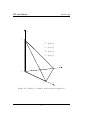
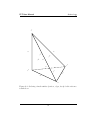
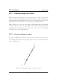
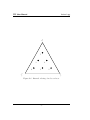
1
FFC User Manual
February 24, 2006
Anders Logg
www.fenics.org
Visit http://www.fenics.org/ for the latest version of this manual.
Send comments and suggestions to [email protected].
Contents
About this manual
7
1 Quickstart
11
1.1
Downloading and installing FFC . . . . . . . . . . . . . . . . . 11
1.2
Compiling Poisson’s equation with FFC . . . . . . . . . . . . . 12
2 Command-line interface
15
2.1
Synopsis . . . . . . . . . . . . . . . . . . . . . . . . . . . . . . 15
2.2
Description . . . . . . . . . . . . . . . . . . . . . . . . . . . . 15
2.3
Options . . . . . . . . . . . . . . . . . . . . . . . . . . . . . . 16
2.3.1
-h, --help . . . . . . . . . . . . . . . . . . . . . . . . 16
2.3.2
-v, --version . . . . . . . . . . . . . . . . . . . . . . 16
2.3.3
-l language, --language language . . . . . . . . . 16
2.3.4
-d debuglevel, --debug debuglevel . . . . . . . . . 16
2.3.5
-f option . . . . . . . . . . . . . . . . . . . . . . . . . 17
3
FFC User Manual
Anders Logg
2.3.6
-f no-gpl . . . . . . . . . . . . . . . . . . . . . . . . . 17
2.3.7
-f blas . . . . . . . . . . . . . . . . . . . . . . . . . . 17
3 Python interface
19
3.1
compile(forms, ...) . . . . . . . . . . . . . . . . . . . . . . 20
3.2
build(forms, ...) . . . . . . . . . . . . . . . . . . . . . . . 20
3.3
write(forms, ...) . . . . . . . . . . . . . . . . . . . . . . . 20
3.4
writeFiniteElement(element, ...) . . . . . . . . . . . . . 21
4 Form language
23
4.1
Overview . . . . . . . . . . . . . . . . . . . . . . . . . . . . . . 23
4.2
The form language as a Python extension . . . . . . . . . . . . 25
4.3
Basic data types
4.4
. . . . . . . . . . . . . . . . . . . . . . . . . 25
4.3.1
FiniteElement . . . . . . . . . . . . . . . . . . . . . . 25
4.3.2
MixedElement . . . . . . . . . . . . . . . . . . . . . . . 27
4.3.3
BasisFunction . . . . . . . . . . . . . . . . . . . . . . 27
4.3.4
Function . . . . . . . . . . . . . . . . . . . . . . . . . 28
4.3.5
Constant . . . . . . . . . . . . . . . . . . . . . . . . . 29
4.3.6
Index . . . . . . . . . . . . . . . . . . . . . . . . . . . 30
4.3.7
Identity . . . . . . . . . . . . . . . . . . . . . . . . . 30
Scalar operators . . . . . . . . . . . . . . . . . . . . . . . . . . 31
4.4.1
Scalar addition: + . . . . . . . . . . . . . . . . . . . . . 31
4
FFC User Manual
4.5
4.6
4.7
Anders Logg
4.4.2
Scalar subtraction: - . . . . . . . . . . . . . . . . . . . 31
4.4.3
Scalar multiplication: * . . . . . . . . . . . . . . . . . . 31
4.4.4
Scalar division: / . . . . . . . . . . . . . . . . . . . . . 32
Vector operators
. . . . . . . . . . . . . . . . . . . . . . . . . 32
4.5.1
Component access: v[i] . . . . . . . . . . . . . . . . . 32
4.5.2
Scalar product: dot(v, w) . . . . . . . . . . . . . . . . 33
4.5.3
Vector product: cross(v, w) . . . . . . . . . . . . . . 33
4.5.4
Matrix product: mult(A, B)
4.5.5
Transpose: transp(A) . . . . . . . . . . . . . . . . . . 33
4.5.6
Trace: trace(A) . . . . . . . . . . . . . . . . . . . . . 34
4.5.7
Vector length: len(v) . . . . . . . . . . . . . . . . . . 34
4.5.8
Rank: rank(v) . . . . . . . . . . . . . . . . . . . . . . 34
4.5.9
Vectorization: vec(v) . . . . . . . . . . . . . . . . . . 34
. . . . . . . . . . . . . . 33
Differential operators . . . . . . . . . . . . . . . . . . . . . . . 35
4.6.1
Scalar partial derivative: D(v, i) . . . . . . . . . . . . 35
4.6.2
Gradient: grad(v) . . . . . . . . . . . . . . . . . . . . 35
4.6.3
Divergence: div(v) . . . . . . . . . . . . . . . . . . . . 36
4.6.4
Rotation: rot(v) . . . . . . . . . . . . . . . . . . . . . 36
Integrals . . . . . . . . . . . . . . . . . . . . . . . . . . . . . . 36
4.7.1
Integration over the interior: *dx . . . . . . . . . . . . 36
4.7.2
Integration over the boundary: *ds . . . . . . . . . . . 37
5
FFC User Manual
Anders Logg
4.8
Index notation . . . . . . . . . . . . . . . . . . . . . . . . . . . 37
4.9
User-defined operators . . . . . . . . . . . . . . . . . . . . . . 38
5 Examples
41
5.1
The mass matrix . . . . . . . . . . . . . . . . . . . . . . . . . 41
5.2
Poisson’s equation
5.3
Vector-valued Poisson . . . . . . . . . . . . . . . . . . . . . . . 43
5.4
The strain-strain term of linear elasticity . . . . . . . . . . . . 43
5.5
The nonlinear term of Navier–Stokes . . . . . . . . . . . . . . 44
5.6
The heat equation
5.7
Mixed formulation of Stokes . . . . . . . . . . . . . . . . . . . 46
. . . . . . . . . . . . . . . . . . . . . . . . 42
. . . . . . . . . . . . . . . . . . . . . . . . 45
A Reference elements
49
A.1 The reference triangle . . . . . . . . . . . . . . . . . . . . . . . 49
A.2 The reference tetrahedron . . . . . . . . . . . . . . . . . . . . 51
A.3 Ordering of degrees of freedom . . . . . . . . . . . . . . . . . . 52
A.3.1 Mesh entities . . . . . . . . . . . . . . . . . . . . . . . 52
A.3.2 Ordering among mesh entities . . . . . . . . . . . . . . 55
A.3.3 Internal ordering on edges . . . . . . . . . . . . . . . . 55
A.3.4 Alignment of edges . . . . . . . . . . . . . . . . . . . . 56
A.3.5 Internal ordering on faces . . . . . . . . . . . . . . . . 56
A.3.6 Alignment of faces . . . . . . . . . . . . . . . . . . . . 56
6
FFC User Manual
Anders Logg
B Installation
59
B.1 Installing from source . . . . . . . . . . . . . . . . . . . . . . . 59
B.1.1 Dependencies and requirements . . . . . . . . . . . . . 59
B.1.2 Downloading the source code . . . . . . . . . . . . . . 61
B.1.3 Installing the compiler . . . . . . . . . . . . . . . . . . 62
B.1.4 Compiling the demos . . . . . . . . . . . . . . . . . . . 62
B.1.5 Verifying the generated code . . . . . . . . . . . . . . . 63
B.2 Debian package . . . . . . . . . . . . . . . . . . . . . . . . . . 63
C Contributing code
65
C.1 Creating a patch . . . . . . . . . . . . . . . . . . . . . . . . . 65
C.2 Sending patches . . . . . . . . . . . . . . . . . . . . . . . . . . 67
C.3 Applying a patch (maintainers) . . . . . . . . . . . . . . . . . 67
C.4 License agreement . . . . . . . . . . . . . . . . . . . . . . . . . 68
D License
69
7
About this manual
This manual is currently being written. As a consequence, some sections
may be incomplete or inaccurate.
Intended audience
This manual is written both for the beginning and the advanced user. There
is also some useful information for developers. More advanced topics are
treated at the end of the manual or in the appendix.
Typographic conventions
• Code is written in monospace (typewriter) like this.
• Commands that should be entered in a Unix shell are displayed as
follows:
# ./configure
# make
Commands are written in the dialect of the bash shell. For other shells,
such as tcsh, appropriate translations may be needed.
9
FFC User Manual
Anders Logg
Enumeration and list indices
Throughout this manual, elements xi of sets {xi } of size n are enumarated
from i = 0 to i = n − 1. Derivatives in Rn are enumerated similarly:
∂/∂x0 , ∂/∂x1 , . . . , ∂/∂xn−1 .
Contact
Comments, corrections and contributions to this manual are most welcome
and should be sent to
[email protected]
10
Chapter 1
Quickstart
This chapter demonstrates how to get started with FFC, including downloading and installing the latest version of FFC, and compiling Poisson’s
equation. These topics are discussed in more detail elsewhere in this manual. In particular, see Appendix B for detailed installation instructions and
Chapter 4 for a detailed discussion of the form language.
1.1
Downloading and installing FFC
The latest version of FFC can be found on the FEniCS web page:
http://www.fenics.org/
The following commands illustrate the installation process, assuming that
you have downloaded release 0.1.0 of FFC:
# tar zxfv ffc-0.1.0.tar.gz
# cd ffc-0.1.0
# python setup.py install
11
FFC User Manual
Anders Logg
Make sure that you download the latest release (which is not 0.1.0).
Note that you may need to be root on your system to do the last step.
You may also need to install the Python packages FIAT and Numeric. (See
Appendix B for detailed instructions.)
1.2
Compiling Poisson’s equation with FFC
The discrete variational (finite element) formulation of Poisson’s equation,
−∆u = f , reads: Find U ∈ Vh such that
a(v, U ) = L(v) ∀v ∈ V̂h ,
(1.1)
with (V̂h , Vh ) a pair of suitable function spaces (the test and trial spaces).
The bilinear form a : V̂h × Vh → R is given by
Z
a(v, U ) =
∇v · ∇U dx
(1.2)
Ω
and the linear form L : V̂h → R is given by
Z
L(v) =
v f dx.
(1.3)
Ω
To compile the pair of forms (a, L) into code that can called to assemble the
linear system Ax = b corresponding to the variational problem (1.1) for a
pair of discrete function spaces, specify the forms in a text file with extension
.form, e.g. Poisson.form, as follows:
element = FiniteElement(‘‘Lagrange’’, ‘‘triangle’’, 1)
v = BasisFunction(element)
U = BasisFunction(element)
f = Function(element)
a = dot(grad(v), grad(U))*dx
L = f*v*dx
12
FFC User Manual
Anders Logg
The example is given for piecewise linear finite elements in two dimensions,
but other choices are available, including arbitrary order Lagrange elements
in two and three dimensions.
To compile the pair of forms implemented in the file Poisson.form, call the
compiler on the command-line as follows:
# ffc Poisson.form
This generates the file Poisson.h which implements the forms in C++ for
inclusion in DOLFIN. For help on the ffc command, including compilation
for other systems than DOLFIN, type ffc -h or man ffc.
13
Chapter 2
Command-line interface
The command-line interface of FFC is documented by the man page for FFC,
which can be read by the command
man ffc
on any system where FFC has been installed. A copy of this documentation
is included below for convenience.
2.1
Synopsis
ffc [-h] [-l language] [-d debuglevel] [-f option] input.form
2.2
Description
The FEniCS Form Compiler FFC accepts as input one or more files each
specifying one or more multilinear forms and compiles the given forms into
15
FFC User Manual
Anders Logg
efficent low-level code for automatic assembly of the tensors representing the
multilinear forms. In particular, FFC compiles a pair of bilinear and linear
forms defining a variational problem into code that can be used to efficiently
assemble the corresponding linear system.
By default, FFC generates C++ code for DOLFIN, but this can be changed
by specifying a different output language (option -l). It is also possible to
add new output languages to FFC.
2.3
2.3.1
Options
-h, --help
Display help text and exit.
2.3.2
-v, --version
Display version number and exit.
2.3.3
-l language, --language language
Specify output language, one of dolfin (default), latex, raw, ase or xml.
2.3.4
-d debuglevel, --debug debuglevel
Specify debug level (default is 0).
16
FFC User Manual
2.3.5
Anders Logg
-f option
Specify code generation options. The list of options available depends on
the specified language (format). Current options include -f no-gpl and -f
blas described in detail below.
2.3.6
-f no-gpl
Don’t add GPL license to generated code. This option has only effect when
compiling with -ldolfin.
2.3.7
-f blas
Generate code that uses BLAS to compute tensor products. This option has
only effect when compiling with -ldolfin.
17
Chapter 3
Python interface
FFC provides a Python interface in the form of a standard Python module.
The following example demonstrates how to define and compile the variational problem for Poisson’s equation in a Python script:
from ffc import *
element = FiniteElement(‘‘Lagrange’’, ‘‘triangle’’, 1)
v = BasisFunction(element)
U = BasisFunction(element)
f = Function(element)
a = dot(grad(v), grad(U))*dx
L = f*v*dx
compile([a, L])
At the basic level, the only difference between the command-line interface
and the Python interface is that the function compile must be called when
using the Python interface.
19
FFC User Manual
Anders Logg
In addition to the function compile, the Python interface provides the functions build, write and writeFiniteElement. These functions are documented below.
Documentation can also be accessed from within Python. To read the documentation for the function compile, run the following commands in a Python
shell:
from ffc import *
help(compile)
3.1
compile(forms, ...)
This function takes as argument a form or list of forms and compiles it into
low-level code for assembly. Calling this function is equivalent to first calling
build followed by write.
3.2
build(forms, ...)
This function takes as argument a form or list of forms and does preprocessing
of the forms (including computation of the reference tensor), but does not
generate any code.
3.3
write(forms, ...)
This function takes a preprocessed form or list of forms and generates code.
Note that build must be called before write:
forms = build([a, L])
write(forms)
20
FFC User Manual
3.4
Anders Logg
writeFiniteElement(element, ...)
This function generates code for a given FiniteElement. Use this function
if you just want to generate code for a finite element (including mapping of
nodes and nodal points):
element = FiniteElement(‘‘Lagrange’’, ‘‘triangle’’, 1)
writeFiniteElement(element)
21
Chapter 4
Form language
FFC uses a flexible and extensible language to define and process multilinear
forms. In this chapter, we give the details of this form language and present a
number of examples to illustrate the use of the form language in applications.
4.1
Overview
A form is expressed using a combination of basic data types and operators.
FFC compiles a given multilinear form
a : Vh1 × Vh2 × · · · × Vhr → R
(4.1)
into code that can be used to compute the corresponding tensor
Ai = a(φ1i1 , φ2i2 , . . . , φrir ).
(4.2)
In the form language, a multilinear form is defined by first specifying the set
of function spaces, Vh1 , Vh2 , . . . , Vhr , and then expressing the multilinear form
in terms of the basis functions of these functions spaces.
A function space is defined in the form language through a FiniteElement,
and a corresponding basis function is represented as a BasisFunction. The
23
FFC User Manual
Anders Logg
following code defines a pair of basis functions v and U for a first-order Lagrange finite element on triangles:
element = FiniteElement(‘‘Lagrange’’, ‘‘triangle’’, 1)
v = BasisFunction(element)
U = BasisFunction(element)
The two basis functions can now be used to define a bilinear form:
a = v*D(U, 0)*dx
corresponding to the mathematical notation
Z
∂U
a(v, U ) =
v
dx.
Ω ∂x0
(4.3)
Note the order of the argument list of the multilinear form is determined by
the order in which basis functions are declared, not by the order in which they
appear in the form. Thus, both a = v*D(U, 0)*dx and a = D(U, 0)*v*dx
define the same multilinear form.
The arity of a multilinear form is determined by the number of basis functions
appearing in the definition
R of the form. Thus, a = v*U*dx defines a bilinear
form, namely a(v,
R U ) = Ω v u dx, whereas L = v*f*dx defines a linear form,
namely L(v) = Ω v f dx.
In the case of a bilinear form, the first of the two basis functions is referred
to as the test function and the second is referred to as the trial function.
Not every expression is a valid multilinear form. The following list explains
some of the basic rules that must be obeyed in the definition of a form:
• A form must be linear in each of its arguments; otherwise it is not a
multilinear form. Thus, a = v*v*U*dx is not a valid form, since it is
quadratic in v.
24
FFC User Manual
Anders Logg
• The value of a form must be a scalar. Thus, if v is a vector-valued
basis function (see below), then L = v*dx is not a valid form, since the
value of the form is not a scalar.
• The integrand of a form must be integrated exactly once. Thus, neither
a = v*u nor a = v*u*dx*dx are valid forms.
4.2
The form language as a Python extension
The FFC form language is built on top of Python. This is true both when
calling FFC as a compiler from the command-line or when calling the FFC
compiler from within a Python program. Through the addition of a collection
of basic data types and operators, FFC allows a form to be specified in a
language that is close to the mathematical notation. Since the form language
is built on top of Python, any Python code is valid in the definition of a form
(but not all Python code defines a multilinear form). In particular, comments
(lines starting with #) and functions (keyword def, see Section 4.9 below)
are allowed in the definition of a form.
4.3
4.3.1
Basic data types
FiniteElement
The data type FiniteElement represents a finite element on a triangle or
tetrahedron. A FiniteElement is declared by specifying the type of element,
the underlying shape, the polynomial order and, optionally, the number of
vector components:
element = FiniteElement(type, shape, <degree>, <num components>)
The argument type is a string and possible values include:
25
FFC User Manual
Anders Logg
• ‘‘Lagrange’’, representing a standard Lagrange finite element for continuous piecewise polynomial functions;
• ‘‘Discontinuous Lagrange’’, representing a discontinuous Lagrange
finite element for discontinuous piecewise polynomial functions;
• ‘‘Vector Lagrange’’, representing a standard vector Lagrange finite
element for continuous piecewise polynomial vector-valued functions;
• ‘‘Discontinuous vector Lagrange’’, representing a discontinuous
Lagrange finite element for discontinuous piecewise polynomial vectorvalued functions.
The argument shape is a string and possible values include:
• ‘‘triangle’’, representing a triangle in R2 ;
• ‘‘tetrahedron’’, representing a tetrahedron in R3 .
The argument order is an integer specifying the polynomial order of the
finite element. Note that the minimal order for Lagrange finite elements is
one, whereas the minimal order for discontinuous Lagrange finite elements is
zero.
The argument num components is optional and specifies the number of vector
components for a vector-valued element. If not specified, the number of vector components is assumed to be the same the dimension d of the underlying
shape.
Note that more than one FiniteElement can be declared and used in the
definition of a form. The following example declares two elements, one linear
and one quadratic Lagrange finite element:
P1 = FiniteElement(‘‘Lagrange’’, ‘‘tetrahedron’’, 1)
P2 = FiniteElement(‘‘Lagrange’’, ‘‘tetrahedron’’, 2)
26
FFC User Manual
4.3.2
Anders Logg
MixedElement
The data type MixedElement represents a mixed finite element on a triangle
or tetrahedron. The function space of a mixed finite element is defined as the
direct sum of the function spaces of a given list of elements. A MixedElement
is declared by specifying a list of FiniteElements:
mixed_element = FiniteElement([e0, e1, ...])
Alternatively, a MixedElement can be created as the sum of a sequence of
FiniteElements. The following example illustrates how to create a TaylorHood element (quadratic velocity and linear pressure):
P2 = FiniteElement("Vector Lagrange", "triangle", 2)
P1 = FiniteElement("Lagrange", "triangle", 1)
TH = P2 + P1
4.3.3
BasisFunction
The data type BasisFunction represents a basis function on a given finite
element. A BasisFunction must be declared from a previously declared
FiniteElement:
v = BasisFunction(element)
Note that more than one BasisFunction can be declared from the same
FiniteElement.
Note that the order in which BasisFunctions are declared is important. The
order determines the order of arguments to the multilinear form. Thus, for a
bilinear form a(v, U ), the test function v should be declared before the trial
function U :
27
FFC User Manual
Anders Logg
v = BasisFunction(element)
U = BasisFunction(element)
For a MixedElement, the function BasisFunctions can be used to construct
tuples of BasisFunctions, as illustrated here for a mixed Taylor-Hood element:
(v, q) = BasisFunctions(TH)
(U, P) = BasisFunctions(TH)
4.3.4
Function
The data type Function represents a function belonging to a given finite
element space, that is, a linear combination of basis functions of the finite
element space. A Function must be declared from a previously declared
FiniteElement:
f = Function(element)
Note that more than one BasisFunction can be declared from the same
FiniteElement. The following example declares two BasisFunctions and
one Function from the same FiniteElement:
v = BasisFunction(element)
U = BasisFunction(element)
f = Function(element)
Function is used to represent user-defined functions, including right-hand
sides, variable coefficients and stabilization terms. FFC treats each Function
as a linear combination of basis functions with unknown coefficients. It is
the responsibility of the user or the system for which the form is compiled to
28
FFC User Manual
Anders Logg
supply the values of the coefficients at run-time. In the case of DOLFIN, the
coefficients are automatically computed from a given user-defined function
during the assembly of a form.
Note that the order in which Functions are declared is important. The
code generated by FFC accepts as arguments a list of functions that should
correspond to the Functions appearing in the form in the order they have
been declared.
For a MixedElement, the function Functions can be used to construct tuples
of Functions, as illustrated here for a mixed Taylor-Hood element:
(f, g) = Functions(TH)
4.3.5
Constant
The data type Constant represents a constant scalar value that is unknown
at compile-time. A Constant is declared without any arguments:
c = Constant()
Just as with Functions, it is the responsibility of the user or the system for
which the form is compiled to supply the value of the constant at run-time.
In the case of DOLFIN, a constant is automatically assigned a value from a
given user-defined variable.
Note that the order in which Constants are declared is important. The
code generated by FFC accepts as arguments a list of constants that should
correspond to the Constants appearing in the form in the order they have
been declared.
29
FFC User Manual
4.3.6
Anders Logg
Index
The data type Index represents an index used for subscripting derivatives
or taking components of vector-valued functions. If an Index is declared
without any arguments,
i = Index()
a free Index is created, representing an index range determined by the context; if used to subscript a vector-valued BasisFunction or a Function, the
range is given by the number of vector dimensions n, and if used to subscript
a derivative, the range is given by the dimension d of the underlying shape
of the finite element space. As we shall see below, indices can be a powerful
tool when used to define forms in tensor notation.
An Index can also be fixed, meaning that the value of the index remains
constant:
i = Index(0)
When using the command-line interface to FFC, a sequence of free indices
are automatically declared for convenience: i, j, k, l, m, n. Note however
that a user is free to declare new indices with other names or even reuse these
variables for other things than indices.
4.3.7
Identity
The data type Identity represents an n × n unit matrix of given size n. An
Identity is declared by specifying the dimension n:
I = Identity(n)
30
FFC User Manual
4.4
Anders Logg
Scalar operators
The basic operators used to define a form are scalar addition, subtraction
and multiplication. Note the absence of division which is intentionally left
out (but see the comment below).
4.4.1
Scalar addition: +
Scalar addition is supported for all scalar-valued basic data types, thus
including BasisFunction, Function, Constant and expressions involving
these data types.
In addition, unary plus is supported for all basic data types.
4.4.2
Scalar subtraction: -
Scalar subtraction is supported for all scalar-valued basic data types, thus
including BasisFunction, Function, Constant and expressions involving
these data types.
In addition, unary minus is supported for all basic data types.
4.4.3
Scalar multiplication: *
Scalar multiplication is supported for all scalar-valued basic data types, thus
including BasisFunction, Function, Constant and expressions involving
these data types.
31
FFC User Manual
4.4.4
Anders Logg
Scalar division: /
Division is not allowed in the definition of a form. This is because division
by a BasisFunction in the definition of a form does not result in a valid
multilinear form, since a multilinear form must be linear in each of its arguments. Division by Functions and Constants may be implemented in future
versions of FFC.
4.5
Vector operators
Vectors are defined in the form language using Python’s built-in list type.
This means that all list operations such as slicing, list comprehension etc.
are supported. There is one exception to this rule, namely vector-valued
BasisFunctions and Functions, which are not lists (but can be made into
lists using the operator vec discussed below). The operators listed below
support all objects which are logically vectors, thus including both Python
lists and vector-valued expressions.
4.5.1
Component access: v[i]
Brackets [] are used to pick a given component of a logically vector-valued
expression. Thus, if v is a vector-valued expression, then v[0] represents a
function corresponding to the first component of (the values of) v. Similarly,
if i is an Index (free or fixed), then v[i] represents a function corresponding
to component i of (the values of) v.
32
FFC User Manual
4.5.2
Anders Logg
Scalar product: dot(v, w)
The operator dot accepts as arguments two logically vector-valued expressions and returns the scalar product (dot product) of the two vectors:
dot(v, w) ↔ v · w =
n−1
X
v i wi .
(4.4)
i=0
Note that this operator is only defined for vectors of equal length.
4.5.3
Vector product: cross(v, w)
The operator cross accepts as arguments two logically vector-valued expressions and returns a vector which is the cross product (vector product) of the
two vectors:
cross(v, w) ↔ v × w = (v1 w2 − v2 w1 , v2 w0 − v0 w2 , v0 w1 − v1 w0 ).
(4.5)
Note that this operator is only defined for vectors of length three.
4.5.4
Matrix product: mult(A, B)
The operator mult accepts as arguments two matrices (or more generally,
tensors) and returns the matrix (tensor) product.
4.5.5
Transpose: transp(A)
The operator transp accept as argument a matrix and return the transpose
of the given matrix:
transp(A)[i][j] ↔ (A> )ij = Aji .
33
(4.6)
FFC User Manual
4.5.6
Anders Logg
Trace: trace(A)
The operator trace accepts as argument a square matrix A and returns its
trace, that is, the sum of its diagonal elements:
trace(A) ↔ trace(A) =
n−1
X
Aii .
(4.7)
i=0
4.5.7
Vector length: len(v)
The operator len accepts as argument a logically vector-valued expression
and returns its length (the number of vector components).
4.5.8
Rank: rank(v)
The operator rank returns the rank of the given argument. The rank of an
expression is defined as the number of times the operator [] can be applied
to the expression before a scalar is obtained. Thus, the rank of a scalar is
zero, the rank of a vector is one and the rank of a matrix is two.
4.5.9
Vectorization: vec(v)
The operator vec is used to create a Python list object from a logically
vector-valued expression. This operator has no effect on expressions which
are already lists. Thus, if v is a vector-valued BasisFunction, then vec(v)
returns a list of the components of v. This can be used to define forms in
terms of standard Python list operators or Python Numeric array operators.
The operator vec does not have to be used if the form is defined only in
terms of the basic operators of the form language.
34
FFC User Manual
4.6
4.6.1
Anders Logg
Differential operators
Scalar partial derivative: D(v, i)
The basic differential operator is the scalar partial derivative D. This differential operator accepts as arguments a scalar or logically vector-valued
expression v together with a coordinate direction i and returns the partial
derivative of the expression in the given coordinate direction:
D(v, i) ↔
∂v
.
∂xi
(4.8)
Alternatively, the member function dx can be used. For v an expression, the
two expressions D(v, i) and v.dx(i) are equivalent, but note that only the
operator D works on vector-valued expressions that are defined in terms of
Python lists.
4.6.2
Gradient: grad(v)
The operator grad accepts as argument an expression v and returns its gradient. If v is scalar, the result is a vector containing the partial derivatives
in the coordinate directions:
grad(v) ↔ grad(v) = ∇v = (
∂v ∂v
∂v
,
,...,
).
∂x0 ∂x1
∂xd−1
(4.9)
If v is logically vector-valued, the result is a matrix with rows given by the
gradients of each component:
grad(v)[i][j] ↔ (grad(v))ij = (∇v)ij =
∂vi
.
∂xj
(4.10)
Thus, if v is scalar-valued, then grad(grad(v)) returns the Hessian of v,
and if v is vector-valued, then grad(v) is the Jacobian of v.
35
FFC User Manual
4.6.3
Anders Logg
Divergence: div(v)
The operator div accepts as argument a logically vector-valued expression
and returns its divergence:
div(v) ↔ div(v) = ∇ · v =
d−1
X
∂vi
.
∂x
i
i=0
(4.11)
Note that the length n of the vector v must be equal to the dimension d of
the underlying shape of the FiniteElement defining the function space for v.
4.6.4
Rotation: rot(v)
The operator rot accepts as argument a logically vector-valued expression
and returns its rotation:
rot(v) ↔ rot(v) = ∇ × v = (
∂v1 ∂v0
∂v2 ∂v1
∂v0
∂v2
−
,
−
,
−
). (4.12)
∂x1 ∂x2 ∂x2 ∂x0 ∂x0 ∂x1
Note that this operator is only defined for vectors of length three.
Alternatively, the name curl can be used for this operator.
4.7
Integrals
Each term of a valid form expression must be a scalar-valued expression
integrated exactly once. Integrals are expressed through multiplication with
a measure, representing either an integral over the interior of the domain Ω
or the boundary ∂Ω of Ω.
4.7.1
Integration over the interior: *dx
A measure for integration over the interior of Ω is created as follows:
36
FFC User Manual
Anders Logg
dx = Integral(‘‘interior’’)
If v is a scalar-valued expression, then the integral of v over the interior of
Ω is written as v*dx.
When using the command-line interface to FFC, the measure dx is automatically declared as an integral over the interior of Ω. Note however that a user
is free to declare measures with other names or even reuse the variable dx
for something else.
4.7.2
Integration over the boundary: *ds
A measure for integration over the boundary of Ω is created as follows:
ds = Integral(‘‘boundary’’)
If v is a scalar-valued expression, then the integral of v over the boundary
of Ω is written as v*ds.
When using the command-line interface to FFC, the measure ds is automatically declared as an integral over the boundary of Ω. Note however that a
user is free to declare measures with other names or even reuse the variable
ds for something else.
At this point, complete support has not been added to FFC for boundary
integrals, which means that all boundary integrals are currently evaluated to
zero.
4.8
Index notation
FFC supports index notation, which is often a convenient way to express
forms. The basic principle of index notation is that summation is implicit
37
FFC User Manual
Anders Logg
over indices repeated twice in each term of an expression. The following
examples illustrate the index notation, assuming that each of the variables i
and j have been declared as a free Index:
v[i]*w[i] ↔
D(v, i)*D(w, i) ↔
D(v[i], i) ↔
D(v[i], j)*D(w[i], j) ↔
n−1
X
i=0
d−1
X
i=0
d−1
X
v i wi ,
(4.13)
∂v ∂w
= ∇v · ∇w,
∂xi ∂xi
(4.14)
∂vi
= ∇ · v,
∂xi
(4.15)
∂vi ∂wi
.
∂xj ∂xj
(4.16)
i=0
n−1
d−1
XX
i=0 j=0
Index notation is used internally by FFC to represent multilinear forms and in
most cases, FFC is capable of generating an efficient tensor representation of
any given expression. However, in some cases index notation might generate
more efficient code.
4.9
User-defined operators
A user may define new operators, using standard Python syntax. As an
example, consider the strain operator ² of linear elasticity, defined by
1
²(v) = (∇v + (∇v)> ).
2
(4.17)
This operator can be implemented as a function using the Python def keyword:
def epsilon(v):
return 0.5*(grad(v) + transp(grad(v)))
38
FFC User Manual
Anders Logg
Alternatively, using the shorthand lambda notation, the strain operator may
be defined as follows:
epsilon = lambda v: 0.5*(grad(v) + transp(grad(v)))
39
Chapter 5
Examples
The following examples illustrate basic usage of the form language for the
definition of a collection of standard multilinear forms. We assume that
dx has been declared as an integral over the interior of Ω and that both i
and j have been declared as a free Index, which is always the case if the
command-line interface is used.
The examples presented below can all be found in the subdirectory src/demo
of the FFC source tree.
5.1
The mass matrix
As a first example, consider the bilinear form corresponding to a mass matrix,
Z
a(v, U ) =
v U dx,
(5.1)
Ω
which can be implemented in FFC as follows:
element = FiniteElement("Lagrange", "triangle", 1)
v = BasisFunction(element)
41
FFC User Manual
Anders Logg
U = BasisFunction(element)
a = v*U*dx
This example is implemented in the file Mass.form in the collection of demonstration forms included with the FFC source distribution.
5.2
Poisson’s equation
The bilinear and linear forms form for Poisson’s equation,
Z
a(v, U ) =
∇v · ∇U dx,
Ω
Z
L(v) =
v f dx,
(5.2)
(5.3)
Ω
can be implemented as follows:
element = FiniteElement("Lagrange", "triangle", 1)
v = BasisFunction(element)
U = BasisFunction(element)
f = Function(element)
a = dot(grad(v), grad(U))*dx
L = v*f*dx
Alternatively, index notation can be used to express the scalar product:
a = D(v, i)*D(U, i)*dx
This example is implemented in the file Poisson.form in the collection of
demonstration forms included with the FFC source distribution.
42
FFC User Manual
5.3
Anders Logg
Vector-valued Poisson
The bilinear and linear forms for a system of (independent) Poisson equations,
Z
a(v, U ) =
∇v : ∇U dx,
(5.4)
Ω
Z
v · f dx,
(5.5)
L(v) =
Ω
with v, U and f vector-valued can be implemented as follows:
element = FiniteElement(‘‘Vector Lagrange’’, ‘‘triangle’’, 1)
v = BasisFunction(element)
U = BasisFunction(element)
f = Function(element)
a = dot(grad(v), grad(U))*dx
L = dot(v, f)*dx
Alternatively, index notation may be used:
a = D(v[i], j)*D(U[i], j)*dx
L = v[i]*f[i]*dx
This example is implemented in the file PoissonSystem.form in the collection of demonstration forms included with the FFC source distribution.
5.4
The strain-strain term of linear elasticity
The strain-strain term of linear elasticity,
Z
a(v, U ) =
²(v) : ²(U ) dx,
Ω
43
(5.6)
FFC User Manual
Anders Logg
where
1
²(v) = (∇v + (∇v)> )
2
can be implemented as follows:
(5.7)
element = FiniteElement("Vector Lagrange", "tetrahedron", 1)
v = BasisFunction(element)
U = BasisFunction(element)
def epsilon(v):
return 0.5*(grad(v) + transp(grad(v)))
a = dot(epsilon(v), epsilon(U))*dx
Alternatively, index notation can be used to define the form:
a = 0.25*(D(v[i], j) + D(v[j], i))*
(D(U[i], j) + D(U[j], i))*dx
This example is implemented in the file Elasticity.form in the collection
of demonstration forms included with the FFC source distribution.
5.5
The nonlinear term of Navier–Stokes
The bilinear form for fixed-point iteration on the nonlinear term of the incompressible Navier–Stokes equations,
Z
a(v, U ) =
v · ((w · ∇)U ) dx,
(5.8)
Ω
with w the frozen velocity from a previous iteration, can be conveniently
implemented using index notation as follows:
44
FFC User Manual
Anders Logg
element = FiniteElement("Vector Lagrange", "tetrahedron", 1)
v = BasisFunction(element)
U = BasisFunction(element)
w = Function(element)
a = v[i]*w[j]*D(U[i], j)*dx
This example is implemented in the file NavierStokes.form in the collection
of demonstration forms included with the FFC source distribution.
5.6
The heat equation
Discretizing the heat equation,
u̇ − ∇ · (c∇u) = f,
(5.9)
in time using the dG(0) method (backward Euler), we obtain the following
variational problem for the discrete solution U = U (x, t): Find U n = U (·, tn )
with U n−1 = U (·, tn−1 ) given such that
Z
Z
Z
1
n
n−1
n
(U − U ) v dx +
c ∇U · ∇v dx =
f n v dx
(5.10)
kn Ω
Ω
Ω
for all test functions v, where k = tn − tn−1 denotes the time step . In the
example below, we implement this variational problem with piecewise linear
test and trial functions, but other choices are possible (just choose another
finite element).
Rewriting the variational problem in the standard form a(v, U ) = L(v) for
all v, we obtain the following pair of bilinear and linear forms:
Z
Z
n
n
(5.11)
a(v, U ) =
v U dx + kn c v · ∇U n dx,
Ω
Ω
Z
Z
n−1
L(v) =
vU
dx + kn v f n dx,
(5.12)
Ω
Ω
which can be implemented as follows:
45
FFC User Manual
Anders Logg
element = FiniteElement("Lagrange", "triangle", 1)
v
U1
U0
c
f
k
=
=
=
=
=
=
BasisFunction(element)
BasisFunction(element)
Function(element)
Function(element)
Function(element)
Constant()
#
#
#
#
#
#
Test function
Value at t_n
Value at t_n-1
Heat conductivity
Heat source
Time step
a = v*U1*dx + k*c*dot(grad(v), grad(U1))*dx
L = v*U0*dx + k*v*f*dx
5.7
Mixed formulation of Stokes
To solve Stokes’ equations,
− ∆u + ∇p = f,
∇ · u = 0,
(5.13)
(5.14)
we write the variational problem in standard form a(v, U ) = L(v) for all v
to obtain the following pair of bilinear and linear forms:
Z
a(v, (U, P )) =
∇v : ∇U − (∇ · v) P + q (∇ · U ) dx,
(5.15)
ZΩ
L(v) =
v · f dx.
(5.16)
Ω
Using a mixed formulation with Taylor-Hood elements, this can be implemented as follows:
P2 = FiniteElement("Vector Lagrange", "triangle", 2)
P1 = FiniteElement("Lagrange", "triangle", 1)
TH = P2 + P1
(v, q) = BasisFunctions(TH)
46
FFC User Manual
Anders Logg
(U, P) = BasisFunctions(TH)
f = Function(P2)
a = (dot(grad(v), grad(U)) - div(v)*P + q*div(U))*dx
L = dot(v, f)*dx
47
Appendix A
Reference elements
A.1
The reference triangle
The reference triangle (Figure A.1) is defined by the following three vertices:
v 0 = (0, 0),
v 1 = (1, 0),
v 2 = (0, 1).
(A.1)
Note that this corresponds to a counter-clockwise orientation of the vertices
in the plane.
The edges of the reference triangle are ordered following the convention that
edge ei should be opposite to vertex v i for i = 0, 1, 2, with the vertices of
each edge ordered to give a counter-clockwise orientation of the triangle in
the plane:
e0 : (v 1 , v 2 ),
e1 : (v 2 , v 0 ),
e2 : (v 0 , v 1 ).
49
(A.2)
FFC User Manual
Anders Logg
x1
v2
v 0 = (0, 0)
v 1 = (1, 0)
PSfrag replacements
v 2 = (0, 1)
x0
v0
v1
Figure A.1: Physical coordinates of the reference triangle.
v2
e1
e0
v0
e2
PSfrag replacements
v1
Figure A.2: Ordering of mesh entities (vertices and edges) for the reference
triangle.
50
FFC User Manual
A.2
Anders Logg
The reference tetrahedron
The reference tetrahedron (Figure A.3) is defined by the following four vertices:
v0
v1
v2
v4
= (0, 0, 0),
= (1, 0, 0),
= (0, 1, 0),
= (0, 0, 1).
(A.3)
The faces of the reference tetrahedron are ordered following the convention
that face f i should be opposite to vertex v i for i = 0, 1, 2, 3, with the vertices
of each face ordered to give a counter-clockwise orientation of each face as
seen from the outside of the tetrahedron and the first vertex of face f i given
by vertex v i+1 mod 4 :
f0
f1
f2
f3
: (v 1 , v 3 , v 2 ),
: (v 2 , v 3 , v 0 ),
: (v 3 , v 1 , v 0 ),
: (v 0 , v 1 , v 2 ).
(A.4)
The edges of the reference tetrahedron are ordered following the convention
that edges e0 , e1 , e2 should correspond to the edges of the reference triangle.
Edges e3 , e4 , e5 all ending up at vertex v 3 are ordered based on their first
vertex:
e0
e1
e2
e3
e4
e5
: (v 1 , v 2 ),
: (v 2 , v 0 ),
: (v 0 , v 1 ),
: (v 0 , v 3 ),
: (v 1 , v 3 ),
: (v 2 , v 3 ).
(A.5)
The ordering of vertices on faces implicitly defines an ordering of edges on
51
FFC User Manual
Anders Logg
faces by identifying an edge on a face with the opposite vertex on the face:
f0
f1
f2
f3
: (e5 , e0 , e4 ),
: (e3 , e1 , e5 ),
: (e2 , e3 , e4 ),
: (e0 , e1 , e2 ).
(A.6)
Note that the ordering of edges on f 3 is the same as the ordering of edges
on the reference triangle. Also note that the internal ordering of vertices
on edges does not always follow the orientation of the face (which is not
possible).
A.3
Ordering of degrees of freedom
The local and global orderings of degrees of freedom or nodes are obtained
by associating each node with a mesh entity, locally and globally.
A.3.1
Mesh entities
We distinguish between mesh entities of different topological dimensions:
vertices
edges
faces
cells
topological
topological
topological
topological
dimension
dimension
dimension
dimension
0
1
2
2 or 3
A cell can be either a triangle or a tetrahedron depending on the type of
mesh. For a mesh consisting of triangles, the mesh entities involved are
vertices, edges and cells, and for a mesh consisting of tetrahedrons, the mesh
entities involved are vertices, edges, faces and cells.
52
FFC User Manual
Anders Logg
x2
v3
v 0 = (0, 0, 0)
v 1 = (1, 0, 0)
v 2 = (0, 1, 0)
v 3 = (0, 0, 1)
PSfrag replacements
v2
x1
v0
v1
x0
Figure A.3: Physical coordinates of the reference tetrahedron.
53
FFC User Manual
Anders Logg
v3
PSfrag replacements e3
e5
f
1
f0
f2
e4
v2
e1
v0
f3
e0
e
2
v1
Figure A.4: Ordering of mesh entities (vertices, edges, faces) for the reference
tetrahedron.
54
FFC User Manual
A.3.2
Anders Logg
Ordering among mesh entities
With each mesh entity, there can be associated zero or more nodes and the
nodes are ordered locally and globally based on the topological dimension of
the mesh entity with which they are associated. Thus, any nodes associated
with vertices are ordered first and nodes associated with cells last.
If more than one node is associated with a single mesh entity, the internal
ordering of the nodes associated with the mesh entity becomes important, in
particular for edges and faces, where the nodes of two adjacent cells sharing
a common edge or face must lign up.
A.3.3
Internal ordering on edges
For edges containing more than one node, the nodes are ordered in the direction from the first vertex (ve0 ) of the edge to the second vertex (ve1 ) of the
edge as in Figure A.5.
ve1
2
1
PSfrag replacements
0
ve0
Figure A.5: Internal ordering of nodes on edges.
55
FFC User Manual
A.3.4
Anders Logg
Alignment of edges
Depending on the orientation of any given cell, an edge on the cell may be
aligned or not aligned with the corresponding edge on the reference cell if the
vertices of the cell are mapped to the reference cell. We define the alignment
of an edge with respect to a cell to be 0 if the edge is aligned with the
orientation of the reference cell and 1 otherwise.
Example 1: The alignment of the first edge (e0 ) on a triangle is 0 if the
first vertex of the edge is the second vertex (v 1 ) of the triangle.
Example 2: The alignment of the second edge (e1 ) on a tetrahedron is 0 if
the first vertex of the edge is the third vertex (v 2 ) of the tetrahedron.
If two cells share a common edge and the edge is aligned with one of the cells
and not the other, we must reverse the order in which the local nodes are
mapped to global nodes on one of the two cells. As a convention, the order
is kept if the alignment is 0 and reversed if the alignment is 1.
A.3.5
Internal ordering on faces
For faces containing more than one node, the ordering of nodes is nested
going from the first to the third vertex and in each step going from the first
to the second vertex as in Figure A.6.
A.3.6
Alignment of faces
There are six different ways for a face to be aligned on a tetrahedron; there are
three ways to pick the first edge of the face, and once the first edge is picked,
there are two ways to pick the second edge. To define an alignment of faces as
an integer between 0 and 5, we compare the ordering of edges on a face with
the ordering of edges on the corresponding face on the reference tetrahedron.
If the first edge of the face matches the first edge on the corresponding face
on the reference tetrahedron and also the second edge matches the second
edge on the reference tetrahedron, then the alignment is 0. If only the first
56
FFC User Manual
Anders Logg
vf2
PSfrag replacements
5
3
0
4
1
2
vf0
vf1
Figure A.6: Internal ordering of nodes on faces.
57
FFC User Manual
Anders Logg
edge matches, then the alignment is 1. We similarly define alignments 2, 3
by matching the first and second edges with the second and third edges on
the corresponding face on the reference tetrahedron, and alignments 4, 5 by
matching the first and second edges with the third and first edges on the
corresponding face on the reference tetrahedron.
Example 1: The alignment of the first face of a tetrahedron is 0 if the first
edge of the face is edge number 5 and the second edge is edge number 0.
Example 2: The alignment of the first face of a tetrahedron is 1 if the first
edge of the face is edge number 5 and the second edge is not edge number 0.
(It must then be edge number 4.)
Example 3: The alignment of the first face of a tetrahedron is 4 if the first
edge of the face is edge number 4 and the second edge is edge number 5.
Example 4: The alignment of the first face of a tetrahedron is 5 if the first
edge of the face is edge number 4 and the second edge is not edge number 5.
(It must then be edge number 0.)
58
Appendix B
Installation
The source code of FFC is portable and should work on any system with a
standard Python installation. Questions, bug reports and patches concerning
the installation should be directed to the FFC mailing list at the address
[email protected]
FFC must currently be installed directly from source, but effort is underway
to provide precompiled Debian packages of FFC and other FEniCS components.
B.1
B.1.1
Installing from source
Dependencies and requirements
FFC depends on a number of libraries that need to be installed on your
system. These libraries include FIAT and the Python Numeric module. In
addition, you need to have a working Python installation on your system.
59
FFC User Manual
Anders Logg
Installing Python
FFC is developed for Python 2.4, but might also work with Python 2.3.
To check which version of Python you have installed, issue the command
python -V:
# python -V
Python 2.4.1
If Python is not installed on your system, it can be downloaded from
http://www.python.org/
Follow the installation instructions for Python given on the Python web page.
For Debian users, the package to install is python2.4.
Installing Numeric
In addition to Python itself, FFC depends on the Python package Numeric,
which is used by FFC to process multidimensionall arrays (tensors). Python
Numeric can be downloaded from
http://www.scipy.org/
For Debian users, the package to install is python2.4-numeric.
Installing FIAT
FFC depends on the latest version of FIAT, which can be downloaded from
60
FFC User Manual
Anders Logg
http://www.fenics.org/
FIAT is used by FFC to create and evaluate finite element basis functions
and quadrature rules. The installation instructions for FIAT are similar to
those for FFC given in detail below.
In addition, you will need to install the Python package LinearAlgebra, which
may already be included in your installation of Python Numeric. For Debian
users, the package to install is python2.4-numeric-ext.
B.1.2
Downloading the source code
The latest release of FFC can be obtained as a tar.gz archive in the download section at
http://www.fenics.org/
Download the latest release of FFC, for example ffc-0.1.0.tar.gz, and
unpack using the command
# tar zxfv ffc-0.1.0.tar.gz
This creates a directory ffc-0.1.0 containing the FFC source code.
If you want the very latest version of FFC, there is also a version named
ffc-cvs-current.tar.gz which provides a snapshot of the current CVS
version of FFC, updated automatically from the CVS repository each hour.
This version may contain features not yet present in the latest release, but
may also be less stable and even not work at all.
61
FFC User Manual
B.1.3
Anders Logg
Installing the compiler
FFC follows the standard for Python packages. Enter the source directory
of FFC, and issue the following command:
# python setup.py install
This will install the FFC Python package in a subdirectory called ffc in
the default location for user-installed Python packages (usually in the directory /usr/lib/python2.4/site-packages). In addition, the compiler
executable (a Python script) will be installed in the default directory for
user-installed Python scripts (usually in /usr/bin).
To see a list of optional parameters to the installation script, type
# python setup.py install --help
If you don’t have root access to the system you are using, you can pass the
--home option to the installation script to install FFC in your home directory:
# mkdir ~/local
# python setup.py install --home ~/local
This installs the FFC package in the directory ~/local/lib/python and the
FFC executable in ~/local/bin. If you use this option, make sure to set
the environment variable PYTHONPATH to ~/local/lib/python and to add
~/local/bin to the PATH environment variable.
B.1.4
Compiling the demos
To test your installation of FFC, enter the subdirectory src/demo and compile some of the demonstration forms. With FFC installed on your system,
just type
62
FFC User Manual
Anders Logg
# ffc Poisson.form
to compile the bilinear and linear forms for Poisson’s equation. This will
generate a C++ header file called Poisson.h that can be used with DOLFIN
to implement a solver for Poisson’s equation. Adding the flag -l latex
generates output in LATEX format:
# ffc -l latex Poisson.form
# latex Poisson.tex
# xdvi Poisson.dvi
It is also possible to compile the forms in src/demo without needing to install
FFC on your system. In that case, you need to supply the path to the FFC
executable:
# ../bin/ffc Poisson.form
B.1.5
Verifying the generated code
To verify the output generated by the compiler, run the script verify from
within the FFC source tree:
# scripts/verify
This script compiles all forms found in src/demo and compares the output
with previously compiled forms in src/reference.
B.2
Debian package
In preparation.
63
Appendix C
Contributing code
If you have created a new module, fixed a bug somewhere, or have made a
small change which you want to contribute to FFC, then the best way to do
so is to send us your contribution in the form of a patch. A patch is a file
which describes how to transform a file or directory structure into another.
The patch is built by comparing a version which both parties have against
the modified version which only you have.
C.1
Creating a patch
The tool used to create a patch is called diff and the tool used to apply
the patch is called patch. These tools are free software and are standard on
most Unix systems.
Here’s an example of how it works. Start from the latest release of FFC,
which we here assume is release 0.1.0. You then have a directory structure
under ffc-0.1.0 where you have made modifications to some files which you
think could be useful to other users.
1. Clean up your modified directory structure to remove temporary and
binary files which will be rebuilt anyway:
65
FFC User Manual
Anders Logg
# make clean
2. From the parent directory, rename the FFC directory to something else:
# mv ffc-0.1.0 ffc-0.1.0-mod
3. Unpack the version of FFC that you started from:
# tar zxfv ffc-0.1.0.tar.gz
4. You should now have two FFC directory structures in your current
directory:
# ls
ffc-0.1.0
ffc-0.1.0-mod
5. Now use the diff tool to create the patch:
# diff -u --new-file --recursive ffc-0.1.0
ffc-0.1.0-mod > ffc-<identifier>-<date>.patch
written as one line, where <identifier> is a keyword that can be used
to identify the patch as coming from you (your username, last name,
first name, a nickname etc) and <date> is today’s date in the format
yyyy-mm-dd.
6. The patch now exists as ffc-<identifier>-<date>.patch and can
be distributed to other people who already have ffc-0.1.0 to easily
create your modified version. If the patch is large, compressing it with
for example gzip is advisable:
# gzip ffc-<identifier>-<date>.patch
66
FFC User Manual
C.2
Anders Logg
Sending patches
Patch files should be sent to the FFC mailing list at the address
[email protected]
Include a short description of what your patch accomplishes. Small patches
have a better chance of being accepted, so if you are making a major contribution, please consider breaking your changes up into several small selfcontained patches if possible.
C.3
Applying a patch (maintainers)
Let’s say that a patch has been built relative to FFC release 0.1.0. The
following description then shows how to apply the patch to a clean version
of release 0.1.0.
1. Unpack the version of FFC which the patch is built relative to:
# tar zxfv ffc-0.1.0.tar.gz
2. Check that you have the patch ffc-<identifier>-<date>.patch and
the FFC directory structure in the current directory:
# ls
ffc-0.1.0
ffc-<identifier>-<date>.patch
Unpack the patch file using gunzip if necessary.
3. Enter the FFC directory structure:
# cd ffc-0.1.0
67
FFC User Manual
Anders Logg
4. Apply the patch:
# patch -p1 < ../ffc-<identifier>-<date>.patch
The option -p1 strips the leading directory from the filename references
in the patch, to match the fact that we are applying the patch from
inside the directory. Another useful option to patch is --dry-run
which can be used to test the patch without actually applying it.
5. The modified version now exists as ffc-0.1.0.
C.4
License agreement
By contributing a patch to FFC, you agree to license your contributed code
under the GNU General Public License (a condition also built into the GPL
license of the code you have modified). Before creating the patch, please
update the author and date information of the file(s) you have modified
according to the following example:
__author__ = ‘‘Anders Logg ([email protected])’’
__date__ = ‘‘2004-11-17 -- 2005-09-09’’
__copyright__ = ‘‘Copyright (c) 2004, 2005 Anders Logg’’
__license__ = ‘‘GNU GPL Version 2’’
# Modified by Johan Jansson 2005.
As a rule of thumb, the original author of a file holds the copyright.
68
Appendix D
License
FFC is licensed under the GNU General Public License (GPL) version 2,
included verbatim below.
GNU GENERAL PUBLIC LICENSE
Version 2, June 1991
Copyright (C) 1989, 1991 Free Software Foundation, Inc.
59 Temple Place, Suite 330, Boston, MA 02111-1307 USA
Everyone is permitted to copy and distribute verbatim copies
of this license document, but changing it is not allowed.
Preamble
The licenses for most software are designed to take away your
freedom to share and change it. By contrast, the GNU General Public
License is intended to guarantee your freedom to share and change free
software--to make sure the software is free for all its users. This
General Public License applies to most of the Free Software
Foundation’s software and to any other program whose authors commit to
using it. (Some other Free Software Foundation software is covered by
the GNU Library General Public License instead.) You can apply it to
your programs, too.
When we speak of free software, we are referring to freedom, not
price. Our General Public Licenses are designed to make sure that you
have the freedom to distribute copies of free software (and charge for
69
FFC User Manual
Anders Logg
this service if you wish), that you receive source code or can get it
if you want it, that you can change the software or use pieces of it
in new free programs; and that you know you can do these things.
To protect your rights, we need to make restrictions that forbid
anyone to deny you these rights or to ask you to surrender the rights.
These restrictions translate to certain responsibilities for you if you
distribute copies of the software, or if you modify it.
For example, if you distribute copies of such a program, whether
gratis or for a fee, you must give the recipients all the rights that
you have. You must make sure that they, too, receive or can get the
source code. And you must show them these terms so they know their
rights.
We protect your rights with two steps: (1) copyright the software, and
(2) offer you this license which gives you legal permission to copy,
distribute and/or modify the software.
Also, for each author’s protection and ours, we want to make certain
that everyone understands that there is no warranty for this free
software. If the software is modified by someone else and passed on, we
want its recipients to know that what they have is not the original, so
that any problems introduced by others will not reflect on the original
authors’ reputations.
Finally, any free program is threatened constantly by software
patents. We wish to avoid the danger that redistributors of a free
program will individually obtain patent licenses, in effect making the
program proprietary. To prevent this, we have made it clear that any
patent must be licensed for everyone’s free use or not licensed at all.
The precise terms and conditions for copying, distribution and
modification follow.
GNU GENERAL PUBLIC LICENSE
TERMS AND CONDITIONS FOR COPYING, DISTRIBUTION AND MODIFICATION
0. This License applies to any program or other work which contains
a notice placed by the copyright holder saying it may be distributed
under the terms of this General Public License. The "Program", below,
refers to any such program or work, and a "work based on the Program"
means either the Program or any derivative work under copyright law:
that is to say, a work containing the Program or a portion of it,
either verbatim or with modifications and/or translated into another
70
FFC User Manual
Anders Logg
language. (Hereinafter, translation is included without limitation in
the term "modification".) Each licensee is addressed as "you".
Activities other than copying, distribution and modification are not
covered by this License; they are outside its scope. The act of
running the Program is not restricted, and the output from the Program
is covered only if its contents constitute a work based on the
Program (independent of having been made by running the Program).
Whether that is true depends on what the Program does.
1. You may copy and distribute verbatim copies of the Program’s
source code as you receive it, in any medium, provided that you
conspicuously and appropriately publish on each copy an appropriate
copyright notice and disclaimer of warranty; keep intact all the
notices that refer to this License and to the absence of any warranty;
and give any other recipients of the Program a copy of this License
along with the Program.
You may charge a fee for the physical act of transferring a copy, and
you may at your option offer warranty protection in exchange for a fee.
2. You may modify your copy or copies of the Program or any portion
of it, thus forming a work based on the Program, and copy and
distribute such modifications or work under the terms of Section 1
above, provided that you also meet all of these conditions:
a) You must cause the modified files to carry prominent notices
stating that you changed the files and the date of any change.
b) You must cause any work that
whole or in part contains or is
part thereof, to be licensed as
parties under the terms of this
you distribute or publish, that in
derived from the Program or any
a whole at no charge to all third
License.
c) If the modified program normally reads commands interactively
when run, you must cause it, when started running for such
interactive use in the most ordinary way, to print or display an
announcement including an appropriate copyright notice and a
notice that there is no warranty (or else, saying that you provide
a warranty) and that users may redistribute the program under
these conditions, and telling the user how to view a copy of this
License. (Exception: if the Program itself is interactive but
does not normally print such an announcement, your work based on
the Program is not required to print an announcement.)
71
FFC User Manual
Anders Logg
These requirements apply to the modified work as a whole. If
identifiable sections of that work are not derived from the Program,
and can be reasonably considered independent and separate works in
themselves, then this License, and its terms, do not apply to those
sections when you distribute them as separate works. But when you
distribute the same sections as part of a whole which is a work based
on the Program, the distribution of the whole must be on the terms of
this License, whose permissions for other licensees extend to the
entire whole, and thus to each and every part regardless of who wrote it.
Thus, it is not the intent of this section to claim rights or contest
your rights to work written entirely by you; rather, the intent is to
exercise the right to control the distribution of derivative or
collective works based on the Program.
In addition, mere aggregation of another work not based on the Program
with the Program (or with a work based on the Program) on a volume of
a storage or distribution medium does not bring the other work under
the scope of this License.
3. You may copy and distribute the Program (or a work based on it,
under Section 2) in object code or executable form under the terms of
Sections 1 and 2 above provided that you also do one of the following:
a) Accompany it with the complete corresponding machine-readable
source code, which must be distributed under the terms of Sections
1 and 2 above on a medium customarily used for software interchange; or,
b) Accompany it with a written offer, valid for at least three
years, to give any third party, for a charge no more than your
cost of physically performing source distribution, a complete
machine-readable copy of the corresponding source code, to be
distributed under the terms of Sections 1 and 2 above on a medium
customarily used for software interchange; or,
c) Accompany it with the information you received as to the offer
to distribute corresponding source code. (This alternative is
allowed only for noncommercial distribution and only if you
received the program in object code or executable form with such
an offer, in accord with Subsection b above.)
The source code for a work means the preferred form of the work for
making modifications to it. For an executable work, complete source
code means all the source code for all modules it contains, plus any
associated interface definition files, plus the scripts used to
72
FFC User Manual
Anders Logg
control compilation and installation of the executable. However, as a
special exception, the source code distributed need not include
anything that is normally distributed (in either source or binary
form) with the major components (compiler, kernel, and so on) of the
operating system on which the executable runs, unless that component
itself accompanies the executable.
If distribution of executable or object code is made by offering
access to copy from a designated place, then offering equivalent
access to copy the source code from the same place counts as
distribution of the source code, even though third parties are not
compelled to copy the source along with the object code.
4. You may not copy, modify, sublicense, or distribute the Program
except as expressly provided under this License. Any attempt
otherwise to copy, modify, sublicense or distribute the Program is
void, and will automatically terminate your rights under this License.
However, parties who have received copies, or rights, from you under
this License will not have their licenses terminated so long as such
parties remain in full compliance.
5. You are not required to accept this License, since you have not
signed it. However, nothing else grants you permission to modify or
distribute the Program or its derivative works. These actions are
prohibited by law if you do not accept this License. Therefore, by
modifying or distributing the Program (or any work based on the
Program), you indicate your acceptance of this License to do so, and
all its terms and conditions for copying, distributing or modifying
the Program or works based on it.
6. Each time you redistribute the Program (or any work based on the
Program), the recipient automatically receives a license from the
original licensor to copy, distribute or modify the Program subject to
these terms and conditions. You may not impose any further
restrictions on the recipients’ exercise of the rights granted herein.
You are not responsible for enforcing compliance by third parties to
this License.
7. If, as a consequence of a court judgment or allegation of patent
infringement or for any other reason (not limited to patent issues),
conditions are imposed on you (whether by court order, agreement or
otherwise) that contradict the conditions of this License, they do not
excuse you from the conditions of this License. If you cannot
distribute so as to satisfy simultaneously your obligations under this
License and any other pertinent obligations, then as a consequence you
73
FFC User Manual
Anders Logg
may not distribute the Program at all. For example, if a patent
license would not permit royalty-free redistribution of the Program by
all those who receive copies directly or indirectly through you, then
the only way you could satisfy both it and this License would be to
refrain entirely from distribution of the Program.
If any portion of this section is held invalid or unenforceable under
any particular circumstance, the balance of the section is intended to
apply and the section as a whole is intended to apply in other
circumstances.
It is not the purpose of this section to induce you to infringe any
patents or other property right claims or to contest validity of any
such claims; this section has the sole purpose of protecting the
integrity of the free software distribution system, which is
implemented by public license practices. Many people have made
generous contributions to the wide range of software distributed
through that system in reliance on consistent application of that
system; it is up to the author/donor to decide if he or she is willing
to distribute software through any other system and a licensee cannot
impose that choice.
This section is intended to make thoroughly clear what is believed to
be a consequence of the rest of this License.
8. If the distribution and/or use of the Program is restricted in
certain countries either by patents or by copyrighted interfaces, the
original copyright holder who places the Program under this License
may add an explicit geographical distribution limitation excluding
those countries, so that distribution is permitted only in or among
countries not thus excluded. In such case, this License incorporates
the limitation as if written in the body of this License.
9. The Free Software Foundation may publish revised and/or new versions
of the General Public License from time to time. Such new versions will
be similar in spirit to the present version, but may differ in detail to
address new problems or concerns.
Each version is given a distinguishing version number. If the Program
specifies a version number of this License which applies to it and "any
later version", you have the option of following the terms and conditions
either of that version or of any later version published by the Free
Software Foundation. If the Program does not specify a version number of
this License, you may choose any version ever published by the Free Software
Foundation.
74
FFC User Manual
Anders Logg
10. If you wish to incorporate parts of the Program into other free
programs whose distribution conditions are different, write to the author
to ask for permission. For software which is copyrighted by the Free
Software Foundation, write to the Free Software Foundation; we sometimes
make exceptions for this. Our decision will be guided by the two goals
of preserving the free status of all derivatives of our free software and
of promoting the sharing and reuse of software generally.
NO WARRANTY
11. BECAUSE THE PROGRAM IS LICENSED FREE OF CHARGE, THERE IS NO WARRANTY
FOR THE PROGRAM, TO THE EXTENT PERMITTED BY APPLICABLE LAW. EXCEPT WHEN
OTHERWISE STATED IN WRITING THE COPYRIGHT HOLDERS AND/OR OTHER PARTIES
PROVIDE THE PROGRAM "AS IS" WITHOUT WARRANTY OF ANY KIND, EITHER EXPRESSED
OR IMPLIED, INCLUDING, BUT NOT LIMITED TO, THE IMPLIED WARRANTIES OF
MERCHANTABILITY AND FITNESS FOR A PARTICULAR PURPOSE. THE ENTIRE RISK AS
TO THE QUALITY AND PERFORMANCE OF THE PROGRAM IS WITH YOU. SHOULD THE
PROGRAM PROVE DEFECTIVE, YOU ASSUME THE COST OF ALL NECESSARY SERVICING,
REPAIR OR CORRECTION.
12. IN NO EVENT UNLESS REQUIRED BY APPLICABLE LAW OR AGREED TO IN WRITING
WILL ANY COPYRIGHT HOLDER, OR ANY OTHER PARTY WHO MAY MODIFY AND/OR
REDISTRIBUTE THE PROGRAM AS PERMITTED ABOVE, BE LIABLE TO YOU FOR DAMAGES,
INCLUDING ANY GENERAL, SPECIAL, INCIDENTAL OR CONSEQUENTIAL DAMAGES ARISING
OUT OF THE USE OR INABILITY TO USE THE PROGRAM (INCLUDING BUT NOT LIMITED
TO LOSS OF DATA OR DATA BEING RENDERED INACCURATE OR LOSSES SUSTAINED BY
YOU OR THIRD PARTIES OR A FAILURE OF THE PROGRAM TO OPERATE WITH ANY OTHER
PROGRAMS), EVEN IF SUCH HOLDER OR OTHER PARTY HAS BEEN ADVISED OF THE
POSSIBILITY OF SUCH DAMAGES.
END OF TERMS AND CONDITIONS
75
Index
BasisFunctions, 27
BasisFunction, 27
Constant, 29
D, 35
FiniteElement, 25
Functions, 28
Function, 28
Identity, 30
Index, 30
MixedElement, 27
cross, 33
curl, 36
div, 36
dot, 33
grad, 35
len, 34
rank, 34
rot, 36
trace, 34
transp, 33
vec, 34
cross product, 33
Debian package, 63
def, 39
dependencies, 59
diff, 65
differential operators, 35
discontinuous Lagrange element, 25
divergence, 36
division, 32
downloading, 11, 61
elasticity, 43
examples, 41
ffc, 13
FIAT, 12
finite elements, 25
fixed-point iteration, 44
form language, 23
functions, 28
GNU General Public License, 69
GPL, 69
gradient, 35
addition, 31
backward Euler, 45
basis functions, 27
boundary measure, 37
heat equation, 45
Hessian, 35
component access, 32
constants, 29
contributing, 65
identity matrix, 30
index notation, 37
indices, 30
77
FFC User Manual
Anders Logg
installation, 11, 59
integrals, 36
interior measure, 36
time-stepping, 45
trace, 34
transpose, 33
Jacobian, 35
user-defined operators, 38
Lagrange element, 25
lambda, 39
license, 68, 69
linear elasticity, 43
vector length, 34
vector operators, 32
vector product, 33
vector rank, 34
vector-valued Poisson, 43
vectorization, 34
man page, 13
mass matrix, 41
matrix product, 33
mixed finite elements, 27
mixed formulation, 46
multiplication, 31
Navier-Stokes, 44
Numeric, 12
partial derivative, 35
patch, 65, 67
Poisson’s equation, 12, 42
Python, 25
quickstart, 11
reference tetrahedron, 51
reference triangle, 49
rotation, 36
scalar operators, 31
scalar product, 33
source code, 61
Stokes’ equations, 46
strain, 43
subscripting, 32
subtraction, 31
Taylor-Hood element, 46
78