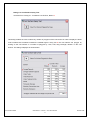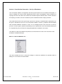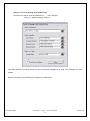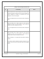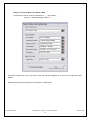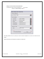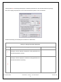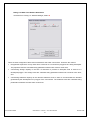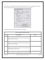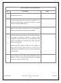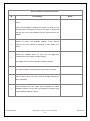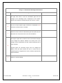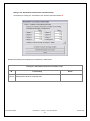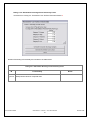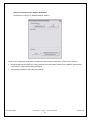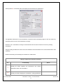
1
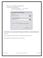
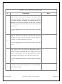
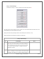
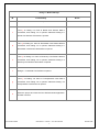
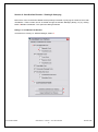
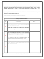
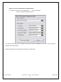
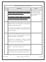
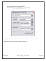
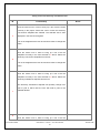
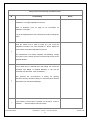
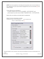
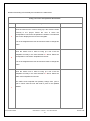
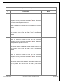
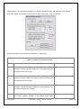
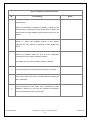
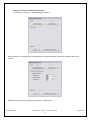
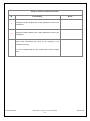
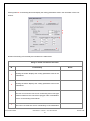
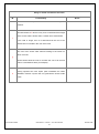
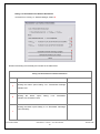
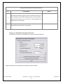
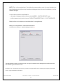
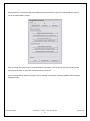
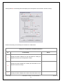
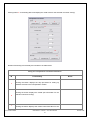
CITY OF CAPE TOWN COST SURFACE MODEL USER MANUAL VOLUME I OF II THE USER INTERFACE Contents Page Notes 2 Section 1: Getting Started 3 Dialog 1.1: Point to Combined Costs Surface Data 4 Dialog 1.2: Module Manager 6 Section 2: Cost Surface Results – Viewing & Querying Dialog 2.1: Combined Cost Surface 8 Dialog 2.2: Cost Surface Query Tool 11 Section 3: Cost Surface Generation – Set Up of Databases 13 Menu 3.1: Point to Databases for . . . 13 Dialog 3.1: Point to Sewage Cost Surface Data 14 Dialog 3.2: Point to Water Cost Surface Data 18 Dialog 3.3: Point to Roads Cost Surface Data 22 Dialog 3.4: Point to Stormwater Cost Surface Data 26 Dialog 3.5: Point to Electricity Cost Surface Data 29 Dialog 3.6: Point to Transportation Cost Data 33 Section 4: Cost Surface Generation – User Inputs Cost Surface Model 8 38 Dialog 4.1 Sewage Cost Surface Generation 38 Dialog 4.2 Water Cost Surface Generation 44 Dialog 4.3 Roads Cost Surface Generation 51 Dialog 4.4 Stormwater Cost Surface Generation 55 Dialog 4.5 Electricity Cost Surface Generation 60 Dialog 4.6 Transport Cost Surface Generation 66 User Manual – Volume I – The User Interface 1 October 2008 Notes: each dialog is headed with it’s name / description in bold and a string of italics directly beneath the name, e.g. Dialog 1.1: Point to Combined Costs Surface Data Accessed from: Automatic At Start Up Menu “Point to Databases for . . .”, Item “Combined” Dialog 1.2: Module Manager, Button f The italics string indicates the “location” at which the dialog can be found, e.g. Dialog 1.1 is activated at start up or through a menu item or via a button on a dialog; grey-shaded lower-case letters on the dialogs indicate areas / functionalities on the dialog that are to be discussed in the text table following the dialog; and the right column of each table is provided for the user to make notes during training and thereafter. Cost Surface Model User Manual – Volume I – The User Interface 2 October 2008 Section 1: Getting Started Open ArcView 3.x. Under menu “File” click item “Open Project…” Navigate to the folder “cost surface model/projects” and open the latest apr file. Cost Surface Model User Manual – Volume I – The User Interface 3 October 2008 Dialog 1.1: Point to Combined Costs Surface Data Accessed from: Automatic At Start Up Menu “Point to Databases for . . .”, Item “Combined” Dialog 1.2: Module Manager, Button f a b c d This dialog opens on start up in order that the application-critical dataset (the cost surface shapefile) and the number of sites per cost surface polygon can be designated at the outset in order that future functionality is not impeded. It is not envisaged that any of the parameters on this dialog need be changed by the user. Details of the dialog’s functionality are included in the table below: Cost Surface Model User Manual – Volume I – The User Interface 4 October 2008 Dialog 1.1: Point to Combined Costs Surface Data ID Functionality Notes Click the search tool in order to bring up a list of all the views currently in the project. Select the view in which the combined cost surface shapefile is situated. The selected view is then displayed in the text box alongside and this view is opened a when querying of the combined cost surface is undertaken (refer to Section 2). It is not envisaged that the user should have need to change this value. Click the search tool in order to bring up a list of all the shapefiles currently in the view selected in a above. Select the b combined cost surface shapefile from the list. It is not envisaged that the user should have need to change this value. Each polygon of the cost surface is approximately 40ha in extent. It has been calculated that this is roughly the size of a 500 unit housing project. All costs to provide bulks to a polygon c are divided by this number in order to arrive at a cost per site. It is not envisaged that the user should have need to change this value. d Clicking this “Next” button will open Dialog 1.2 Module Manager (refer below for details). Cost Surface Model User Manual – Volume I – The User Interface 5 October 2008 Dialog 1.2: Module Manager Accessed from: Dialog 1.1: Point to Combined Costs Surface Data, Button d a b c d e f g h This dialog remains open throughout the user’s session in the Cost Surface Model and enables the user to navigate between the various modules of the model. Clicking each button will open dialogs relevant to that module (refer to Sections 2, 3 & 4). Details of the dialog’s functionality are included in the table below: Dialog 1.2: Module Manager ID Functionality Notes If box y (the “do not show at start up” check box) on Dialog 3.1: a Point to Sewage Cost Surface Data is unchecked, then Dialog 3.1 is opened. Otherwise Dialog 4.1: Sewage Cost Surface Generation is opened. b If box y on Dialog 3.2: Point to Water Cost Surface Data is unchecked, then Dialog 3.2 is opened. Otherwise Dialog 4.2: Cost Surface Model User Manual – Volume I – The User Interface 6 October 2008 Dialog 1.2: Module Manager ID Functionality Notes Water Cost Surface Generation is opened. If box y on Dialog 3.3: Point to Roads Cost Surface Data is c unchecked, then Dialog 3.3 is opened. Otherwise Dialog 4.3: Roads Cost Surface Generation is opened. If box y on Dialog 3.4: Point to Stormwater Cost Surface Data is d unchecked, then Dialog 3.4 is opened. Otherwise Dialog 4.4: Stormwater Cost Surface Generation is opened. If box y on Dialog 3.5: Point to Electricity Cost Surface Data is e unchecked, then Dialog 3.5 is opened. Otherwise Dialog 4.5: Electricity Cost Surface Generation is opened. f Dialog 2.1: Combined Cost Surface is opened. If box y on Dialog 3.6: Point to Transportation Cost Data is g unchecked, then Dialog 3.6 is opened. Otherwise Dialog 4.6: Transportation Cost Surface is opened. h Saves the project and exits the Cost Surface Model application. ArcView is closed. Cost Surface Model User Manual – Volume I – The User Interface 7 October 2008 Section 2: Cost Surface Results – Viewing & Querying Most users of the Cost Surface Model will be primarily interested in querying the results of the model calculations. These results can be accessed through the Module Manager (Dialog 1.2) by clicking button f labelled “Combined”. This opens the dialog as follows: Dialog 2.1: Combined Cost Surface Accessed from: Dialog 1.2: Module Manager, Button f a b c d e Cost Surface Model User Manual – Volume I – The User Interface 8 October 2008 This dialog enables the user to specify the various bulk costs that should be incorporated into the cost surface that is being displayed in the view. Note that the bulk costs for each of the different services has been previously calculated (refer to Section 4) and this process merely sums the individual costs to give a combined cost of the selected bulks. Importantly, the transportation costs have not been included in the combined cost surface as they are an operating type cost as opposed to a bulk cost. Details of the dialog’s functionality are included in the table below: Dialog 2.1: Combined Cost Surface ID Functionality Notes Check or uncheck the box in order to include the Sewage bulk costs in the combined cost surface. a Similarly, this can be done for the Water, Roads, Stormwater Drainage & Electricity bulk costs. Each service’s bulk cost is itself made up of various components and the user is enabled to specify which of these components b should be included in the combined cost surface. If no selection is made then all component costs will be considered if the bulk has been selected (using a above) The user can choose to add the valuation roll land values to the bulks’ combined cost surface. c Cost Surface Model User Manual – Volume I – The User Interface 9 October 2008 Dialog 2.1: Combined Cost Surface ID Functionality Notes Using the selections in a, b and c above, the model calculates and displays the combined cost surface. d It may be necessary for the user to manipulate the legend of the cost surface theme in order for the theme to display intelligibly. e Clicking this button opens Dialog 2.2: Cost Surface Query Tool (refer below for functionality) Cost Surface Model User Manual – Volume I – The User Interface 10 October 2008 Dialog 2.2: Cost Surface Query Tool Accessed from: Dialog 2.1: Combined Cost Surface, Button e f This dialog enables the user to select any number of polygons of the cost surface in order to display the bulks costs numbers that contribute towards the shaded legend. Using tool a the user selects one polygon by clicking on the cost surface or a number of polygons by “click, hold, drag rectangle, release” on the cost surface. The dialog redisplays as shown below: f h g j Cost Surface Model User Manual – Volume I – The User Interface 11 October 2008 Details of the dialog’s functionality are included in the table below: Dialog 2.2: Cost Surface Query Tool ID f g Functionality Notes Tool used to select polygon(s) of Cost Surface theme for query. The selections specified under a, b and c on Dialog 2.1 are listed here with relevant costs. According to the spread of values found in the selection of h polygons, the minimum, maximum and average cost values are displayed. j Given the bulk selection and the polygon selection, the average cost per site is calculated and displayed. Cost Surface Model User Manual – Volume I – The User Interface 12 October 2008 Section 3: Cost Surface Generation – Set Up of Databases The Cost Surface Model is an application that was purpose-written for the eThekwini Municipality. In order to facilitate it’s roll-out across departments and to other municipalities, where possible, the scripting has been soft-coded. This means that eThekwini-specific datasets have not been named in the scripting, but rather, the user is enabled to point to datasets that the scripting accesses. This means that the user has to go through a process of “pointing” to datasets before parameters can be input or calculations can be run. The Cost Surface Model is, however, provided to the Municipality with all relevant datasets “pointed to” and it is not envisaged that the user will have to redo the process. In order to gain a greater understanding of the requirements of the Cost Surface Model (and for completeness), the procedures for designating datasets is detailed in this section. The dialogs on which the datasets are pointed to are accessed via a menu in the view GUI or from the Dialog 1.2 Module Manager: Menu 3.1: Point to Databases for . . . This menu enables the user to access the dialogs on which the datasets are specified. Refer to Dialogs 3.1 to 3.6 below for further details. Cost Surface Model User Manual – Volume I – The User Interface 13 October 2008 Dialog 3.1: Point to Sewage Cost Surface Data Accessed from: Menu “Point to Databases for . . .”, Item “Sewage” Dialog 1.2: Module Manager, Button a a b c d e f y z This dialog enables the user to specify the view and relevant shapefiles to be used in the sewage bulk costs module. Details of the dialog’s functionality are included in the table below: Cost Surface Model User Manual – Volume I – The User Interface 14 October 2008 Dialog 3.1: Point to Sewage Cost Surface Data ID Functionality Notes Click the search tool in order to bring up a list of all the views currently in the project. Select the view in which the sewage cost surface shapefiles are situated. The selected view is then a displayed in the text box alongside. It is not envisaged that the user should have need to change this value. Click the search tool in order to bring up a list of all the shapefiles currently in the view selected in a above. Select the b sewage cost surface shapefile from the list. It is not envisaged that the user should have need to change this value. Click the search tool in order to bring up a list of all the shapefiles currently in the view selected in a above. Select the sewage treatment systems shapefile from the list. Refer to Definition 4.1.a on page 38 for information on treatment systems. c The treatment systems shapefile will possibly change from year to year in which case the user will need to point to the updated dataset. d Cost Surface Model User Manual – Volume I – The User Interface 15 October 2008 Dialog 3.1: Point to Sewage Cost Surface Data ID Functionality Notes Click the search tool in order to bring up a list of all the shapefiles currently in the view selected in a above. Select the sewage pipework zones shapefile from the list. Refer to Definition 4.1.b on page 38 for information on pipework zones. The pipework zones shapefile will possibly change from year to year in which case the user will need to point to the updated dataset. Click the search tool in order to bring up a list of all the shapefiles currently in the view selected in a above. Select the sewage pipework buffers shapefile from the list. e The pipework buffers shapefile will definitely change from year to year in which case the user will need to point to the updated dataset. Click the search tool in order to bring up a list of all the tables currently in the project. Select the sewage pipework costs table from the list. f y The pipework costs will definitely change from year to year in which case the user will need to point to the updated table. If this check box is selected then this Dialog 3.1 cannot be accessed from Dialog 1.2 Module Manager. It can only be accessed from the Menu “Point to Datasets . . .” Cost Surface Model User Manual – Volume I – The User Interface 16 October 2008 Dialog 3.1: Point to Sewage Cost Surface Data ID Functionality Notes This prevents the inconvenience of Dialog 3.1 opening whenever the user accesses Dialog 4.1: Sewage Cost Surface Generation from the Module Manager. If this Dialog 3.1 has been accessed via the Menu “Point to Datasets . . .” then this button will read “Close”. z If the dialog has been accessed via the Module Manager then this button will read “Next >>” and Dialog 4.1: Sewage Cost Surface Generation will be opened when the button is clicked. Cost Surface Model User Manual – Volume I – The User Interface 17 October 2008 Dialog 3.2: Point to Water Cost Surface Data Accessed from: Menu “Point to Databases for . . .”, Item “Water” Dialog 1.2: Module Manager, Button b a b c d e f g h y z This dialog enables the user to specify the view and relevant shapefiles to be used in the water bulk costs module. Details of the dialog’s functionality are included in the table below: Cost Surface Model User Manual – Volume I – The User Interface 18 October 2008 Dialog 3.2: Point to Water Cost Surface Data ID Functionality Notes Click the search tool in order to bring up a list of all the views currently in the project. Select the view in which the water cost surface shapefiles are situated. The selected view is then a displayed in the text box alongside. It is not envisaged that the user should have need to change this value. Click the search tool in order to bring up a list of all the shapefiles currently in the view selected in a above. Select the b water cost surface shapefile from the list. It is not envisaged that the user should need to change this value. Click the search tool in order to bring up a list of all the shapefiles currently in the view selected in a above. Select the c water works zones shapefile from the list. The water works zones shapefile will possibly change from year to year. The user will need to point to the updated dataset. Click the search tool in order to bring up a list of all the shapefiles currently in the view selected in a above. Select the d reservoir zones shapefile from the list. The reservoir zones shapefile will change from year to year in which case the user will need to point to the updated dataset. e Click the search tool in order to bring up a list of all the Cost Surface Model User Manual – Volume I – The User Interface 19 October 2008 Dialog 3.2: Point to Water Cost Surface Data ID Functionality Notes shapefiles currently in the view selected in a above. Select the water trunks buffers shapefile from the list. The water trunks buffers shapefile will definitely change from year to year in which case the user will need to point to the updated dataset. Click the search tool in order to bring up a list of all the shapefiles currently in the view selected in a above. Select the water reticulation buffers shapefile from the list. f The water reticulation buffers shapefile will definitely change from year to year in which case the user will need to point to the updated dataset. Click the search tool in order to bring up a list of all the shapefiles currently in the view selected in a above. Select the g water reticulation shapefile from the list. The water reticulation shapefile will definitely change from year to year. The user will need to point to the updated dataset. Click the search tool in order to bring up a list of all the tables currently in the project. Select the water trunks costs table from h the list. The water trunks costs will definitely change from year to year in which case the user will need to point to the updated table. y If this check box is selected then this Dialog 3.2 cannot be accessed from Dialog 1.2 Module Manager. It can only be accessed from the Menu “Point to Datasets . . .” Cost Surface Model User Manual – Volume I – The User Interface 20 October 2008 Dialog 3.2: Point to Water Cost Surface Data ID Functionality Notes This prevents the inconvenience of Dialog 3.2 opening whenever the user accesses Dialog 4.2: Water Cost Surface Generation from the Module Manager. If this Dialog 3.2 has been accessed via the Menu “Point to Datasets . . .” then this button will read “Close”. z If the dialog has been accessed via the Module Manager then this button will read “Next >>” and Dialog 4.2: Water Cost Surface Generation will be opened when the button is clicked. Cost Surface Model User Manual – Volume I – The User Interface 21 October 2008 Dialog 3.3: Point to Roads Cost Surface Data Accessed from: Menu “Point to Databases for . . .”, Item “Roads” Dialog 1.2: Module Manager, Button c a b c d e f g y z This dialog enables the user to specify the view and relevant shapefiles to be used in the roads bulk costs module. Details of the dialog’s functionality are included in the table below: Cost Surface Model User Manual – Volume I – The User Interface 22 October 2008 Dialog 3.3: Point to Roads Cost Surface Data ID Functionality Notes Click the search tool in order to bring up a list of all the views currently in the project. Select the view in which the roads cost surface shapefiles are situated. The selected view is then a displayed in the text box alongside. It is not envisaged that the user should have need to change this value. Click the search tool in order to bring up a list of all the shapefiles currently in the view selected in a above. Select the b roads cost surface shapefile from the list. It is not envisaged that the user should have need to change this value. Click the search tool in order to bring up a list of all the shapefiles currently in the view selected in a above. Select the c traffic zones shapefile from the list. The traffic zones will possibly change from year to year in which case the user will need to point to the updated dataset. Click the search tool in order to bring up a list of all the shapefiles currently in the view selected in a above. Select the d features shapefile from the list. The features shapefile will change from year to year in which case the user will need to point to the updated dataset e Click the search tool in order to bring up a list of all the Cost Surface Model User Manual – Volume I – The User Interface 23 October 2008 Dialog 3.3: Point to Roads Cost Surface Data ID Functionality Notes shapefiles currently in the view selected in a above. Select the working offsets shapefile from the list. It is not envisaged that the user should have need to change this value. Click the search tool in order to bring up a list of all the shapefiles currently in the view selected in a above. Select the f working routes shapefile from the list. It is not envisaged that the user should have need to change this value. Click the search tool in order to bring up a list of all the tables currently in the project. Select the roads costs table from the list. g The roads costs will definitely change from year to year in which case the user will need to point to the updated table. If this check box is selected then this Dialog 3.3 cannot be accessed from Dialog 1.2 Module Manager. It can only be accessed from the Menu “Point to Datasets . . .” y This prevents the inconvenience of Dialog 3.3 opening whenever the user accesses Dialog 4.3: Roads Cost Surface Generation from the Module Manager. z If this Dialog 3.3 has been accessed via the Menu “Point to Datasets . . .” then this button will read “Close”. Cost Surface Model User Manual – Volume I – The User Interface 24 October 2008 Dialog 3.3: Point to Roads Cost Surface Data ID Functionality Notes If the dialog has been accessed via the Module Manager then this button will read “Next >>” and Dialog 4.3: Roads Cost Surface Generation will be opened when the button is clicked. Cost Surface Model User Manual – Volume I – The User Interface 25 October 2008 Dialog 3.4: Point to Stormwater Cost Surface Data Accessed from: Menu “Point to Databases for . . .”, Item “Stormwater” Dialog 1.2: Module Manager, Button d a b c d e f y z This dialog enables the user to specify the view and relevant shapefiles to be used in the stormwater mitigation bulk costs module. Details of the dialog’s functionality are included in the table below: Cost Surface Model User Manual – Volume I – The User Interface 26 October 2008 Dialog 3.4: Point to Stormwater Cost Surface Data ID Functionality Notes Click the search tool in order to bring up a list of all the views currently in the project. Select the view in which the stormwater cost surface shapefiles are situated. The selected view is then a displayed in the text box alongside. It is not envisaged that the user should have need to change this value. Click the search tool in order to bring up a list of all the shapefiles currently in the view selected in a above. Select the b stormwater cost surface shapefile from the list. It is not envisaged that the user should have need to change this value. Click the search tool in order to bring up a list of all the shapefiles currently in the view selected in a above. Select the c discharge points shapefile from the list. The discharge points shapefile may be updated periodically as new stormwater infrastructure is constructed. Click the search tool in order to bring up a list of all the shapefiles currently in the view selected in a above. Select the river sensitivity polygons shapefile from the list. d The river sensitivity polygons may be updated periodically as more water courses are evaluated to determine their Ecological River Rehabilitation Potential Priority. Cost Surface Model User Manual – Volume I – The User Interface 27 October 2008 Dialog 3.4: Point to Stormwater Cost Surface Data ID Functionality Notes Click the search tool in order to bring up a list of all the The infrastructure condition shapefiles currently in the view selected in a above. Select the category is now an attribute infrastructure condition shapefile from the list. of the “GENERATED PIPES” dataset (f, below) e The infrastructure condition shapefile may be updated periodically as older stormwater infrastructure deteriorates and new infrastructure replaces poor condition infrastructure. Click the search tool in order to bring up a list of all the shapefiles currently in the view selected in a above. Select the generated pipes shapefile from the list. f The generated pipes shapefile holds the algorith-generated pipes. The pipes will be replaced in the shapefile when the cost surface is recalculated. If this check box is selected then this Dialog 3.4 cannot be accessed from Dialog 1.2 Module Manager. It can only be accessed from the Menu “Point to Datasets . . .” y This prevents the inconvenience of Dialog 3.4 opening whenever the user accesses Dialog 4.4: Stormwater Cost Surface Generation from the Module Manager. If this Dialog 3.4 has been accessed via the Menu “Point to Datasets . . .” then this button will read “Close”. z If the dialog has been accessed via the Module Manager then this button will read “Next >>” and Dialog 4.4: Stormwater Cost Surface Generation will be opened when the button is clicked. Cost Surface Model User Manual – Volume I – The User Interface 28 October 2008 Dialog 3.5: Point to Electricity Cost Surface Data Accessed from: Menu “Point to Databases for . . .”, Item “Electricity” Dialog 1.2: Module Manager, Button e a b c d e y z This dialog enables the user to specify the view and relevant shapefiles to be used in the electricity bulk costs module. Details of the dialog’s functionality are included in the table below: Cost Surface Model User Manual – Volume I – The User Interface 29 October 2008 Dialog 3.5: Point to Electricity Cost Surface Data ID Functionality Notes Click the search tool in order to bring up a list of all the views currently in the project. Select the view in which the electricity cost surface shapefiles are situated. The selected view is then a displayed in the text box alongside. It is not envisaged that the user should have need to change this value. Click the search tool in order to bring up a list of all the shapefiles currently in the view selected in a above. Select the b electricity cost surface shapefile from the list. It is not envisaged that the user should have need to change this value. Click the search tool in order to bring up a list of all the shapefiles currently in the view selected in a above. Select the electricity substations shapefile from the list. The electricity substations shapefile will possibly change from year to year in which case the user will need to point to the c d updated dataset. Click the search tool in order to bring up a list of all the Cost Surface Model User Manual – Volume I – The User Interface 30 October 2008 Dialog 3.5: Point to Electricity Cost Surface Data ID Functionality Notes shapefiles currently in the view selected in a above. Select the substations coverage shapefile from the list. Refer to Definition 4.5.a on page 61 for information on substation coverages. It is not envisaged that the user should have need to change this value. Click the search tool in order to bring up a list of all the shapefiles currently in the view selected in a above. Select the transmission line buffers shapefile from the list. e The transmission line buffers shapefile will definitely change from year to year in which case the user will need to point to the updated dataset. If this check box is selected then this Dialog 3.5 cannot be accessed from Dialog 1.2 Module Manager. It can only be accessed from the Menu “Point to Datasets . . .” This prevents the inconvenience of Dialog 3.5 opening y z whenever the user accesses Dialog 4.5: Electricity Cost Surface Generation from the Module Manager. If this Dialog 3.5 has been accessed via the Menu “Point to Datasets . . .” then this button will read “Close”. Cost Surface Model User Manual – Volume I – The User Interface 31 October 2008 Dialog 3.5: Point to Electricity Cost Surface Data ID Functionality Notes If the dialog has been accessed via the Module Manager then this button will read “Next >>” and Dialog 4.5: Electricity Cost Surface Generation will be opened when the button is clicked. Cost Surface Model User Manual – Volume I – The User Interface 32 October 2008 NOTE: Due to the complexities of calculating the transportation costs, the user interface has been disabled and only the output results are displayed when the user clicks button g on the module manager. A cost surface has been calculated for: - all modes of transport (refer to theme “ALL MODES - COST SURFACE”); and - public transport only (refer to theme “PUBLIC TRANSPORT ONLY - COST SURFACE”). Details of the user interface are included below for completeness. Dialog 3.6: Point to Transportation Cost Data Accessed from: Menu “Point to Databases for . . .”, Item “Commuter Costs” Dialog 1.2: Module Manager, Button g a b c d e f g h j y z This dialog enables the user to specify the view and relevant shapefiles to be used in the transportation costs module. Cost Surface Model User Manual – Volume I – The User Interface 33 October 2008 Details of the dialog’s functionality are included in the table below: Dialog 3.6: Point to Transportation Surface Data ID Functionality Notes Click the search tool in order to bring up a list of all the views currently in the project. Select the view in which the transportation cost surface shapefiles are situated. The selected a view is then displayed in the text box alongside. It is not envisaged that the user should have need to change this value. Click the search tool in order to bring up a list of all the shapefiles currently in the view selected in a above. Select the b transportation cost surface shapefile from the list. It is not envisaged that the user should have need to change this value. Click the search tool in order to bring up a list of all the shapefiles currently in the view selected in a above. Select the traffic zones shapefile from the list. The traffic zones shapefile will possibly change from year to year in which case the user will need to point to the updated c dataset. Cost Surface Model User Manual – Volume I – The User Interface 34 October 2008 Dialog 3.6: Point to Transportation Surface Data ID Functionality Notes Click the search tool in order to bring up a list of all the shapefiles currently in the view selected in a above. Select the commuter zones shapefile from the list. d Refer to Definition 4.6.a on page 66 for information on commuter zones. The commuter zones shapefile will possibly change from year to year in which case the user will need to point to the updated dataset. Click the search tool in order to bring up a list of all the shapefiles currently in the view selected in a above. Select the railway stations shapefile from the list. e The railway stations shapefile will possibly change from year to year in which case the user will need to point to the updated dataset. Click the search tool in order to bring up a list of all the shapefiles currently in the view selected in a above. Select the railway stations buffers shapefile from the list. The railway stations buffers shapefile will possibly change from f year to year in which case the user will need to point to the updated dataset. Cost Surface Model User Manual – Volume I – The User Interface 35 October 2008 Dialog 3.6: Point to Transportation Surface Data ID Functionality Notes Click the search tool in order to bring up a list of all the shapefiles currently in the view selected in a above. Select the g working routes shapefile from the list. It is not envisaged that the user should have need to change this value. Click the search tool in order to bring up a list of all the tables currently in the project. Select the origin/destination table from the list. h The origin/destination table will possibly change from year to year in which case the user will need to point to the updated table. Click the search tool in order to bring up a list of all the tables currently in the project. Select the commuter zone table from the j list. The commuter zone table will possibly change from year to year in which case the user will need to point to the updated table. If this check box is selected then this Dialog 3.6 cannot be accessed from Dialog 1.2 Module Manager. It can only be accessed from the Menu “Point to Datasets . . .” y This prevents the inconvenience of Dialog 3.6 opening whenever the user accesses Dialog 4.6: Transportation Cost Surface Generation from the Module Manager. z If this Dialog 3.6 has been accessed via the Menu “Point to Cost Surface Model User Manual – Volume I – The User Interface 36 October 2008 Dialog 3.6: Point to Transportation Surface Data ID Functionality Notes Datasets . . .” then this button will read “Close”. If the dialog has been accessed via the Module Manager then this button will read “Next >>” and Dialog 4.6: Transportation Cost Surface Generation will be opened when the button is clicked. Cost Surface Model User Manual – Volume I – The User Interface 37 October 2008 Section 4: Cost Surface Generation – User Inputs User inputs dialogs are accessed via Dialog 1.2: Module Manager. Dialog 4.1: Sewage Cost Surface Generation Accessed from: Dialog 1.2: Module Manager, Button a a b There are two categories of bulk costs considered for the sewage cost surface. These are the costs of: constructing treatment capacity at the relevant wastewater treatment works in order to accommodate the flows generated by the development of a polygon of the cost surface; and the pipework required to convey sewerage from a cost surface polygon to tie-in to the existing network. The treatment costs are calculated using parameters entered at a treatment systems level. Definition 4.1.a: The treatment systems theme comprises polygons representing areas of the Municipality in which the treatment destination of sewerage is common. The pipework costs are calculated using parameters entered at a pipework zone level. Definition 4.1.b: The pipework zone theme comprises polygons representing areas of the Municipality in which the treatment destination of sewerage is common and the mode whereby the sewerage is transferred to the treatment works is common (i.e. either under gravity or via pumpstation), e.g. the area in which Cost Surface Model User Manual – Volume I – The User Interface 38 October 2008 sewerage can flow under gravity to the Phoenix Wastewater Treatment Works is a pipework zone and the area in which sewerage is / will be pumped to the Phoenix Works is another zone. Clicking button a on the dialog above will display the pipework parameters for the selected pipework zone(s). Note: the scripting will prompt the user to select a pipework zone if none are selected. a b c d e f g h j k m Details of the dialog’s functionality are included in the table below: Dialog 4.1: Sewage Cost Surface Generation ID Functionality Notes Clicking the button displays the pipework costing parameters for a the selected pipework zone(s). Clicking the button displays the treatment costing parameters for b the selected treatment system(s). c The pipe size used to cost the pipework in the pipework zone is displayed in this window. Should it be required to change the Cost Surface Model User Manual – Volume I – The User Interface 39 October 2008 Dialog 4.1: Sewage Cost Surface Generation ID Functionality Notes pipe size, refer to f below. The unit cost per length of pipe of diameter as displayed in c is d read from the sewer pipes cost table (refer to Dialog 3.1: Point to Sewage Cost Surface Data button f). Should the pipework zone under consideration be a pumped e zone, then this option will be enabled and the user can input the value of a suitably-sized pumpstation to pump the flows. f Allows the user to select an alternative pipe size (and hence an alternative unit cost) to be used in the cost calculations. The length of pipe that is costed for each cost surface polygon is the straight line distance between the polygon under consideration and the closest point of the existing sewer network. This distance is measured using buffers generated around the sewer network. g Physical pipes are obviously longer than the straight line distance and this factor allows the user to ensure that the modelled pipes are lengthened to more accurately represent the physical situation. In reality there is a limit as to how long a pipe will be built to tie a h new development into an existing network. It may in fact be more economical to construct a new wastewater treatment works nearer the development than to run a long pipe for many Cost Surface Model User Manual – Volume I – The User Interface 40 October 2008 Dialog 4.1: Sewage Cost Surface Generation ID Functionality Notes kilometres. Checking this box will ensure that the application considers this option (in accordance with the values specified in j & k below). The application uses this number (in conjunction with the j number specified in k below) to determine if it is more economical to build a new treatment works than to construct very long pipes. The application uses this number (in conjunction with the k number specified in j above) to determine if it is more economical to build a new treatment works than to construct very long pipes. Having specified the user inputs (and undertaken the tasks m detailed in Section 5.1) the user can generate the pipework costs for the selected pipework zone(s). Cost Surface Model User Manual – Volume I – The User Interface 41 October 2008 Clicking button b on the dialog will display the treatment parameters for the selected treatment system(s). Note: the scripting will prompt the user to select a treatment system if none are selected. a b c d e f g h Details of the dialog’s functionality are included in the table below: Dialog 4.1: Sewage Cost Surface Generation ID a Functionality Notes Clicking the button displays the pipework costing parameters for the selected pipework zone(s). Clicking the button displays the treatment costing parameters for the selected treatment system(s). b Cost Surface Model User Manual – Volume I – The User Interface 42 October 2008 Dialog 4.1: Sewage Cost Surface Generation ID Functionality Notes The treatment capacity available in the selected treatment system(s) is displayed in Ml/day and in a unit termed “Equivalent Dwelling Units”. c EDU’s are calculated by dividing the capacity in Ml/day by the average sewage generation per site per day (refer f below) and tells the user how many dwelling units the treatment system can support. Similar to c above, the available capacity, or the capacity d remaining for new projects is displayed in both Ml/day and EDU’s. Should the available EDU’s be zero, then the application e calculates the cost to supply treatment capacity. The capital cost to construct capacity is entered. f g The expected sewage generation per site per day is entered. Using e and f above, the cost to provide treatment capacity per site is calculated. Having specified the user inputs (and undertaken the tasks h detailed in Section 5.1) the user can generate the treatment costs for the selected treatment system(s). Cost Surface Model User Manual – Volume I – The User Interface 43 October 2008 Dialog 4.2: Water Cost Surface Generation Accessed from: Dialog 1.2: Module Manager, Button b a b c There are three categories of bulk costs considered for the water cost surface. These are the costs of: the pipework required to convey water from a reservoir to a cost surface polygon that is being developed. The pipework costs are calculated using parameters entered at a reservoir zone level; constructing storage capacity in the form of reservoirs to provide an adequate level of service to a developed polygon. The storage costs are calculated using parameters entered at a reservoir zone level; and constructing treatment capacity at the relevant treatment works in order to accommodate the demand generated by the development of a polygon of the cost surface. The treatment costs are calculated using parameters entered at a water works zones level. Cost Surface Model User Manual – Volume I – The User Interface 44 October 2008 Clicking button a on the dialog above will display the pipework parameters for the selected reservoir zone(s). Note: the scripting will prompt the user to select a reservoir zone if none are selected. a b c d e f g h Details of the dialog’s functionality are included in the table below: Dialog 4.2: Water Cost Surface Generation ID a b c d Functionality Notes Clicking the button displays the pipework costing parameters for the selected reservoir zone(s). Clicking the button displays the storage costing parameters for the selected reservoir zone(s). Clicking the button displays the treatment costing parameters for the selected water works zones(s). The pipe size used to cost the pipework in the reservoir zone is Cost Surface Model User Manual – Volume I – The User Interface 45 October 2008 Dialog 4.2: Water Cost Surface Generation ID Functionality Notes displayed in this window. Should it be required to change the pipe size, refer to f below. The unit cost per length of pipe of diameter as displayed in d is e read from the water trunks cost table (refer to Dialog 3.2: Point to Water Cost Surface Data button h). f Allows the user to select an alternative pipe size (and hence an alternative unit cost) to be used in the cost calculations. The length of pipe that is costed for each cost surface polygon is the straight line distance between the polygon under consideration and the closest point of the existing water trunk network. This distance is measured using buffers generated g around the water trunks. Physical pipes are obviously longer than the straight line distance and this factor allows the user to ensure that the modelled pipes are lengthened to more accurately represent the physical situation. Having specified the user inputs (and undertaken the tasks h detailed in Section 5.2) the user can generate the pipework costs for the selected reservoir zone(s). Cost Surface Model User Manual – Volume I – The User Interface 46 October 2008 Clicking button b on the dialog will display the storage parameters for the selected reservoir zone(s). Note: the scripting will prompt the user to select a reservoir zone if none are selected. a b c j k m n p q Details of the dialog’s functionality are included in the table below: Dialog 4.2: Water Cost Surface Generation ID a b c k Functionality Notes Clicking the button displays the pipework costing parameters for the selected reservoir zone(s). Clicking the button displays the storage costing parameters for the selected reservoir zone(s). Clicking the button displays the treatment costing parameters for the selected water works zones(s). The storage capacity available in the selected reservoir zone(s) Cost Surface Model User Manual – Volume I – The User Interface 47 October 2008 Dialog 4.2: Water Cost Surface Generation ID Functionality Notes is displayed in Ml/day and in a unit termed “Equivalent Dwelling Units”. EDU’s are calculated by dividing the capacity in Ml/day by the average water consumption per site per day (refer n below) and tells the user how many dwelling units the reservoir zone can support. Similar to k above, the available capacity, or the capacity k remaining for new projects is displayed in both Ml/day and EDU’s. Should the available EDU’s be zero, then the application m calculates the cost to supply storage capacity. The capital cost to construct storage capacity is entered. n p The expected water consumption per site per day is entered. Using m and n above, the cost to provide storage capacity per site is calculated. Having specified the user inputs (and undertaken the tasks q detailed in Section 5.2) the user can generate the storage costs for the selected reservoir zone(s). Cost Surface Model User Manual – Volume I – The User Interface 48 October 2008 Clicking button c on the dialog will display the treatment parameters for the selected water works zone(s). Note: the scripting will prompt the user to select a water works zone if none are selected. a b c r s t u v w Details of the dialog’s functionality are included in the table below: Dialog 4.2: Water Cost Surface Generation ID a b c r Functionality Notes Clicking the button displays the pipework costing parameters for the selected reservoir zone(s). Clicking the button displays the storage costing parameters for the selected reservoir zone(s). Clicking the button displays the treatment costing parameters for the selected water works zones(s). The storage capacity available in the selected water works Cost Surface Model User Manual – Volume I – The User Interface 49 October 2008 Dialog 4.2: Water Cost Surface Generation ID Functionality Notes zone(s) is displayed in Ml/day and in a unit termed “Equivalent Dwelling Units”. EDU’s are calculated by dividing the capacity in Ml/day by the average water consumption per site per day (refer u below) and tells the user how many dwelling units the water works zone can support. Similar to r above, the available capacity, or the capacity s remaining for new projects is displayed in both Ml/day and EDU’s. Should the available EDU’s be zero, then the application t calculates the cost to supply treatment capacity. The capital cost to construct treatent capacity is entered. u v The expected water consumption per site per day is entered. Using t and u above, the cost to provide treatment capacity per site is calculated. Having specified the user inputs (and undertaken the tasks w detailed in Section 5.2) the user can generate the treatment costs for the selected water works zone(s). Cost Surface Model User Manual – Volume I – The User Interface 50 October 2008 Dialog 4.3: Roads Cost Surface Generation Accessed from: Dialog 1.2: Module Manager, Button c a b Clicking button a on the dialog above will display the routing parameters used in the calculation of the cost surface. a b c Details of the dialog’s functionality are included in the table below: Cost Surface Model User Manual – Volume I – The User Interface 51 October 2008 Dialog 4.3: Roads Cost Surface Generation ID a b Functionality Notes Clicking the button displays the routing parameters used in the calculations. Clicking the button displays the costing parameters used in the calculations. These three parameters are used by the scripting in the calculation exercise. c It is not envisaged that the user should have need to modify them. Cost Surface Model User Manual – Volume I – The User Interface 52 October 2008 Clicking button b on the dialog above will display the costing parameters used in the calculation of the cost surface. a b d e f g h Details of the dialog’s functionality are included in the table below: Dialog 4.3: Roads Cost Surface Generation ID a b Functionality Notes Clicking the button displays the routing parameters used in the calculations. Clicking the button displays the costing parameters used in the calculations. The user is to enter the unit cost of constructing a bus route type d surfaced road from the cost surface polygon under consideration to tie-in to the existing road network. e The user is to enter the cost of constructing a new intersection Cost Surface Model User Manual – Volume I – The User Interface 53 October 2008 Dialog 4.3: Roads Cost Surface Generation ID Functionality Notes to tie the new development’s access road into the existing road network. The intersection of e above is only to be constructed if the length of the access road is shorter than a certain value entered here. f If the road is longer, then it is assumed that the cost of an intersection is included in the cost of the road. The cost of an access road varies according to the terrain on which it is built. g These factors allow the user to increase the cost of an access road in a mountainous area (for example). Having specified the user inputs (and undertaken the tasks h detailed in Section 5.3) the user can generate the access roads costs. Cost Surface Model User Manual – Volume I – The User Interface 54 October 2008 Dialog 4.4: Stormwater Cost Surface Generation Accessed from: Dialog 1.2: Module Manager, Button d a b c d e f Details of the dialog’s functionality are included in the table below: Dialog 4.4: Stormwater Cost Surface Generation ID a b Functionality Notes Clicking the button opens Dialog 4.4.1: Stormwater Drainage Infrastructure Clicking the button opens Dialog 4.4.2: Stormwater Infrastructure Condition Factor Clicking the button opens Dialog 4.4.3: Stormwater Discharge c Point Sensitivity Cost Surface Model User Manual – Volume I – The User Interface 55 October 2008 Dialog 4.4: Stormwater Cost Surface Generation ID Functionality Notes Generates the lengths of pipes required to drain the low point of d each hexagon to the nearest discharge point of lower elevation. This process should be run only when a new discharge point dataset has been developed. e Recalculates the Stormwater Cost Surface . Dialog 4.4.1: Stormwater Drainage Infrastructure Accessed from: Dialog 4.4: Stormwater Cost Surface Generation Button a a b c d e f g Details of the dialog’s functionality are included in the table overleaf: Cost Surface Model User Manual – Volume I – The User Interface 56 October 2008 Dialog 4.4.1: Stormwater Drainage Infrastructure ID Functionality Notes The pipe size used to cost the stormwater pipe from the a hexagon to the discharge point is displayed in this window. Should it be required to change the pipe size, refer to c below. b c The unit cost per length of pipe of diameter as displayed in b is read from the water trunks cost table. Allows the user to select an alternative pipe size (and hence an alternative unit cost) to be used in the cost calculations. The length of pipe that is costed for each cost surface hexagon is the straight line distance between the lowest point of the hexagon under consideration and the closest discharge point of lower elevation. d Physical pipes are obviously longer than the straight line distance and this factor allows the user to ensure that the modelled pipes are lengthened to more accurately represent the physical situation. e Returns to previous dialog. Cost Surface Model User Manual – Volume I – The User Interface 57 October 2008 Dialog 4.4.2: Stormwater Infrastructure Condition Factor Accessed from: Dialog 4.4: Stormwater Cost Surface Generation Button b Details of the dialog’s functionality are included in the table below: Dialog 4.4.2: Stormwater Infrastructure Condition Factor ID general Functionality Notes Modify factors based on empirical data. Cost Surface Model User Manual – Volume I – The User Interface 58 October 2008 Dialog 4.4.3: Stormwater Discharge Point Sensitivity Factor Accessed from: Dialog 4.4: Stormwater Cost Surface Generation Button c Details of the dialog’s functionality are included in the table below: Dialog 4.4.3: Stormwater Discharge Point Sensitivity Factor ID general Functionality Notes Modify factors based on empirical data. Cost Surface Model User Manual – Volume I – The User Interface 59 October 2008 Dialog 4.5: Electricity Cost Surface Generation Accessed from: Dialog 1.2: Module Manager, Button e a b There are two categories of bulk costs considered for the electricity cost surface. These are the costs of: the transmission lines required to convey electricity from the existing network to a substation positioned at a cost surface polygon that is being developed; constructing substations where they are required. Cost Surface Model User Manual – Volume I – The User Interface 60 October 2008 Clicking button a on the dialog above will display the transmission line parameters. a b c d e f g h j The application determines if a new substation is required for each developing polygon of the cost surface by developing what is known as the substation coverage. Definition 4.5.a: a substation coverage is the theoretical extent to which areas are serviced by existing substations. Polygons falling outside these areas have new substations and transmission lines constructed and their costs assessed. Details of the dialog’s functionality are included in the table below: Dialog 4.5: Electricity Cost Surface Generation ID a b Functionality Notes Clicking the button displays the transmission line costing parameters used in the calculations. Clicking the button displays the substation costing parameters Cost Surface Model User Manual – Volume I – The User Interface 61 October 2008 Dialog 4.5: Electricity Cost Surface Generation ID Functionality Notes used in the calculations. c The user enters an unit cost per km of overhead transmission line. The length of transmission line that is costed for each cost surface polygon is the straight line distance between the polygon under consideration and the closest point of the existing transmission line network. This distance is measured using d buffers generated around the transmission line network. Physical lines are obviously longer than the straight line distance and this factor allows the user to ensure that the modelled lines are lengthened to more accurately represent the physical situation. These numbers are used to generate what is known as the substation coverage. Each substation’s capacity is considered efg and the area in hectares which it can service is calculated. A circle of this area is drawn centred on the substation. This factor allows the reach of the substation coverage to be increased as their actual coverages are not circular in extent. h This factor makes the circles bigger, thus designating more areas as having electricity. j Having specified the parameters, the user clicks the button. A new substation coverage is generated and thereafter each Cost Surface Model User Manual – Volume I – The User Interface 62 October 2008 Dialog 4.5: Electricity Cost Surface Generation ID Functionality Notes polygon of the cost surface is evaluated to see if it falls within the existing coverage. Cost Surface Model User Manual – Volume I – The User Interface 63 October 2008 Clicking button b on the dialog above will display the substation costing parameters. a b m n p q Details of the dialog’s functionality are included in the table below: Dialog 4.5: Electricity Cost Surface Generation ID a b p g Functionality Notes Clicking the button displays the transmission line costing parameters used in the calculations. Clicking the button displays the substation costing parameters used in the calculations. An average cost per site to provide substation capacity is calculated by considering user inputs m and n. All the areas falling outside the substation coverage are Cost Surface Model User Manual – Volume I – The User Interface 64 October 2008 Dialog 4.5: Electricity Cost Surface Generation ID Functionality Notes assigned the average cost per site to provide substation capacity. Cost Surface Model User Manual – Volume I – The User Interface 65 October 2008 NOTE: Due to the complexities of calculating the transportation costs, the user interface has been disabled and only the output results are displayed when the user clicks button g on the module manager. A cost surface has been calculated for: - all modes of transport (refer to theme “ALL MODES - COST SURFACE”); and - public transport only (refer to theme “PUBLIC TRANSPORT ONLY - COST SURFACE”). Details of the user interface are included below for completeness. Dialog 4.6: Transportation Cost Surface Generation Accessed from: Dialog 1.2: Module Manager, Button g a b c The transportation module is built around the concept of commuter zones developed from traffic zones and their related origin-destination matrix. Definition 4.6.a: Commuter zones are any number of merged traffic zones retaining the integrity of the traffic zones’ origin-destination information. Cost Surface Model User Manual – Volume I – The User Interface 66 October 2008 Clicking button a on the dialog above will display the tools necessary to process existing datasets ready for use in the transportation module. a b c Upon receiving new traffic zones or origin-destination information, new commuter zones should be created using the functionality on the panel “Generate Commuter Zones”. Upon receiving railway station information, the functionality on the panel “Generate Railway Data” should be stepped through. Cost Surface Model User Manual – Volume I – The User Interface 67 October 2008 Clicking button b on the dialog above will display the modal splits for the selected commuter zone(s). a b c d e f g h j Details of the dialog’s functionality are included in the table below: Dialog 4.6: Transportation Cost Surface Generation ID a Functionality Notes Clicking the button displays the step processes for setting up datasets relevant to the transportation module. Clicking the button displays the modal split information for the b c selected commuter zone(s). Clicking the button displays the modal costs information for the Cost Surface Model User Manual – Volume I – The User Interface 68 October 2008 Dialog 4.6: Transportation Cost Surface Generation ID Functionality Notes selected commuter zone(s). d Inter-zone travel refers to movement between different commuter zones, i.e. from origin to destination. The different proportions of commuters using different modes of e inter-zone transport in the selected commuter zone(s) are entered by the user. Intra-zone travel refers to travel within the same commuter zone f and is limited to commuters switching mode to train travel only, i.e. how do the people who travel inter-zone by train get to the train station intra-zone – by bus, taxi or walking? The different proportions of commuters using different modes of g intra-zone transport in the selected commuter zone(s) are entered by the user. h j Updates the selected commuter zone(s) with the latest data. Generates transportation routes using the information entered to date. Cost Surface Model User Manual – Volume I – The User Interface 69 October 2008 Clicking button c on the dialog above will display the modal costs for the selected commuter zone(s). a b c k m n Details of the dialog’s functionality are included in the table below: Dialog 4.6: Transportation Cost Surface Generation ID a Functionality Notes Clicking the button displays the step processes for setting up datasets relevant to the transportation module. Clicking the button displays the modal split information for the b c selected commuter zone(s). Clicking the button displays the modal costs information for the Cost Surface Model User Manual – Volume I – The User Interface 70 October 2008 Dialog 4.6: Transportation Cost Surface Generation ID Functionality Notes selected commuter zone(s). k m n The user enters the costs of transport of each mode in the selected commuter zone(s). Updates the selected commuter zone(s) with the latest data. Generates transportation costs using the information entered to date. Cost Surface Model User Manual – Volume I – The User Interface 71 October 2008