1
Using CellProfiler for Automatic
Identification and Measurement of
Biological Objects in Images
UNIT 14.17
Martha S. Vokes1 and Anne E. Carpenter1
1
Broad Institute Imaging Platform, Cambridge, Massachusetts
ABSTRACT
Visual analysis is required to perform many biological experiments, from counting yeast
colonies to measuring the size and shape of individual cells or the intensity of fluorescently labeled proteins within them. This unit outlines the use of CellProfiler, a free,
open-source image analysis tool that extracts quantitative information from biological
images. It includes a step-by-step protocol for automated analysis of the number, color,
and size of yeast colonies growing on agar plates, but the methods can be adapted to
identify and measure any objects in images. The flexibility of the software allows users to
tailor pipelines of adjustable modules to fit different biological experiments, to generate
accurate measurements from dozens or even hundreds of thousands of images. Curr.
C 2008 by John Wiley & Sons, Inc.
Protoc. Mol. Biol. 82:14.17.1-14.17.12. !
Keywords: automatic image analysis ! yeast colonies ! open-source software !
morphology ! colony counting
INTRODUCTION
Many experiments in a biology laboratory involve visual inspection—whether examining
yeast colonies or growth patches on agar plates, or examining live or stained cell samples
by microscopy. Acquiring images and analyzing them automatically with image analysis
software has several advantages over simple visual inspection. It is less tedious, more
objective and quantitative, and, while the set up can be time-consuming, the analysis
itself is usually much faster for large sample sets.
This unit outlines a protocol for the automated counting and analysis of yeast colonies
growing on agar plates; however, the methods described can be adapted to a wide
variety of biological “objects” and can be used to measure a wide variety of features for
each object. The protocol uses the open-source, freely downloadable software package,
CellProfiler. CellProfiler has been validated for a wide variety of biological applications,
including yeast colony counting and classification, cell microarray annotation, yeast patch
assays, cell-cycle classification, mouse tumor quantification, wound healing assays, and
tissue topology measurement (Cowen et al., 2006; Hartwell et al., 2006; Lamprecht et al.,
2007), as well as analysis of fluorescence microscopy images for measurement of cell
size and morphology, cell cycle distributions, fluorescence staining levels, and other
features of individual cells in images (Bailey et al., 2006; Carpenter et al., 2006; Moffat
et al., 2006; Carpenter, 2008).
SETTING UP AND USING CellProfiler
The protocol begins with instructions for downloading the CellProfiler program and an
example “pipeline,” which is shown in Figure 14.17.1. The pipeline is then adjusted so
that it can analyze the experimenter’s own images. Tens of thousands of images can be
routinely analyzed per experiment. In this example, CellProfiler is used to identify and
Current Protocols in Molecular Biology 14.17.1-14.17.12, April 2008
Published online April 2008 in Wiley Interscience (www.interscience.wiley.com).
DOI: 10.1002/0471142727.mb1417s82
C 2008 John Wiley & Sons, Inc.
Copyright !
BASIC
PROTOCOL
In Situ
Hybridization
and Immunohistochemistry
14.17.1
Supplement 82
Using CellProfiler
for Automatic
Image Analysis
Figure 14.17.1 An overview of the CellProfiler example pipeline. The names of the images
created or objects identified appear in italics below each image, whereas the module names
appear in a larger regular font.
14.17.2
Supplement 82
Current Protocols in Molecular Biology
count yeast colonies on each plate, and to measure each colony’s size, shape, texture, and
color. Lastly, instructions are given for analyzing the numerical results, which can be done
within CellProfiler using its built-in data tools, or by exporting the data in a tab-delimited
text file to a spreadsheet program such as Microsoft Excel or more sophisticated analysis
programs such as R (R Development Core Team, 2007).
NOTE: In addition to the Help menu in the main CellProfiler window, there are several
“?” buttons containing more information about how to use CellProfiler. Clicking the
“?” button near the pipeline window will show information about the selected module
within the pipeline. Additionally, the CellProfiler user manual is available in pdf format (http://www.cellprofiler.org/install.htm), and a user forum is available for posting
and reading questions and answers about how to use the software (http://cellprofiler.
org/forum/).
NOTE: There are several options for modifying the appearance of the main CellProfiler
window. To change preferences, click on File > Set Preferences.
Materials
Images of yeast plates to be processed
Images can be taken with a flatbed scanner or digital camera (Dahle et al., 2004;
Memarian et al., 2007; see Critical Parameters for guidance). The images can
be located within subfolders and need not be in a particular order or follow a
particular naming convention. While this example only analyzes one image, it
is possible to analyze hundreds of images on a single computer, or tens of
thousands of images using a computing cluster (see Alternate Protocol). A
variety of file formats are currently readable by CellProfiler, including bmp,
cur, fts, fits, gif, hdf, ico, jpg, jpeg, pbm, pcx, pgm, png, pnm, ppm, ras, tif,
tiff, xwd, dib, mat, fig, and zvi. See Critical Parameters for more information
about acquiring images and image file types.
Computer with at least 1 Gb of RAM and 1 GHz processor (recommended)
CellProfiler is available for Macintosh, Windows, and Unix/Linux. A complete
list of compatible operating systems can be found at http://www.CellProfiler.
org/download.htm. The example image pipeline demonstrated here will be
processed in <1 min/image on a single computer with a 2.4 GHz processor
and 3 Gb RAM. Large image sets (greater than ∼500 images) will likely
require a computing cluster (see Alternate Protocol).
Decompression software (e.g., Winzip, http://www.winzip.com, or Stuffit,
http://www.stuffit.com) for unpacking compressed files
CellProfiler software (see step 1)
Example images and corresponding CellProfiler pipeline (see step 4)
CellProfiler manual (http://www.cellprofiler.org/install.htm)
Download and install CellProfiler software
1. Choose whether to use the regular version or the developer’s version.
Most users will use the regular version (also known as the compiled/Binary version)
suitable for their computing platform (Macintosh, Windows, or Unix/Linux). This version
is free (GPL license) and does not require MATLAB software or a MATLAB license.
Researchers wishing to implement their own image analysis algorithms should download
the developer’s version—i.e., the MATLAB source code. The developer’s version is free
and open-source (GPL license), but does require the installation of MATLAB software
(including its Image Processing Toolbox) and its licenses, not detailed here (Mathworks;
http://www.mathworks.com).
2. Download the chosen version of software from http://www.cellprofiler.org/download.
htm.
CellProfiler downloads in <1 min with a 1 Gbps internet connection.
In Situ
Hybridization
and Immunohistochemistry
14.17.3
Current Protocols in Molecular Biology
Supplement 82
3. Follow the installation instructions from the Web page to install CellProfiler. If difficulties on this step are encountered, consult the installation instructions (http://www.
cellprofiler.org/install.htm), or visit the online forum (http://cellprofiler.org/forum/)
to search if the problem has been encountered previously and resolved.
Download example pipeline and run on example images
4. Download the example image and pipeline called Classified Colonies from
http://www.cellprofiler.org/examples.htm (the downloaded file is called ExampleYeastColonies BT Images.zip). After downloading the file, make sure that it
is decompressed.
Often, decompression occurs automatically. If the downloaded file does not automatically
produce an accompanying folder, decompress the file manually by double clicking it,
which should launch the decompression software.
5. Start CellProfiler as instructed in the installation help.
6. Run the example pipeline, ExampleYeastColonies BT PIPE.mat which was downloaded, on the example images. To do this, follow the instructions in Help > Getting
Started > GettingStarted.
This step shows how processing typically proceeds. A window opens for each module in
the pipeline. Under normal circumstances, more than one image will be processed, and
the module windows will refresh upon completion of each cycle.
See Troubleshooting if an out of memory error message is obtained.
Create test image folders
7. Using the computer’s normal interface, create a test image folder and copy several
test images into it.
These images are used during the setup of the pipeline. To test specific settings thoroughly
and ensure accurate results from the entire experiment, be sure to select a variety of
images from throughout the entire set of images that should be processed. For example,
choose one or two from the beginning, middle, and end, rather than choosing test images
that were collected near each other.
8. Using the computer’s normal interface, create a test output folder.
9. In CellProfiler, set the default image and output folder to be the test image folder
and test output folder, respectively.
Adjust example pipeline for test images
10. Load the desired images using the LoadImages module (see Figs. 14.17.1 and
14.17.2A).
The images need not be named or organized in a particular way to use CellProfiler.
Setting this module tells CellProfiler where to retrieve images and gives each image a
meaningful name that the other modules can access. There are a number of ways images
can be loaded and identified.
When analyzing images of yeast plates, or other samples in which there is only one image
per plate, all you need to do is change the setting to look for text that all of the images have
in common (e.g., a file extension such as.tif). If the images are located within subfolders
inside a main folder, be sure to change the setting Analyze all subfolders within the
selected folder? to Yes. The current example pipeline looks for an exact match between
1.jpg and all files in the default image folder. If the image file names do not have precise
text in common, the Text-regular expressions option might be useful.
Using CellProfiler
for Automatic
Image Analysis
When there are pairs of images from the same plate, there are two basic methods to denote
the image types within CellProfiler. The Order option is used when images are present
in a folder or series of subfolders in repeating order (e.g., Light, Fluorescence, Light,
Fluorescence, etc.). The Text option is used when each type of image has a particular
14.17.4
Supplement 82
Current Protocols in Molecular Biology
Figure 14.17.2 (A) The original plate image. (B) The colonies identified. The colors are arbitrary.
(C) The SubtractedRed image (or the red channel). (D) All identified colonies outlined. (E) The
colonies classified by area. (F) The colonies classified by redness. For the color version of this
figure, go to http://www.currentprotocols.com.
piece of text in the name; for example, when all of the light images contain “LT” and
all of the fluorescence images contain “FL” in the file names. Alternatively, placing two
different LoadImages modules in the pipeline allows one to choose one entire folder of a
particular image type and a separate folder of a different image type (e.g., if “Light” and
“Fluorescence” images are stored in separate folders).
Any number of channels can be analyzed; for example, multiple bright field and fluorescence images. See Help for the LoadImages module for more information.
In Situ
Hybridization
and Immunohistochemistry
14.17.5
Current Protocols in Molecular Biology
Supplement 82
11. Split images using the ColorToGray module.
ColorToGray splits the original color image into three separate images: red, blue, and
green. Each of these images is then converted to an image with varying intensities on a
grayscale. The images are used for separate purposes later in the pipeline. For example,
the red channel will be used to identify all colonies (white and red). A different channel
or combination of channels might be better suited to your own images. This can be
decided based on a visual inspection of which images (red, blue, or green) show the best
contrast for all colonies compared to background, or by using CellProfiler Image Tools
> ShowOrHidePixelData to check the contrast in each channel numerically.
If the original images were collected in grayscale rather than color, it is not necessary to
use the ColorToGray module. Delete this module from the pipeline and adjust the image
names to allow the LoadImages module to feed directly to the next module.
12. Calculate corrections for uneven illumination using the CorrectIllumination
Calculate module.
Because most images are taken with uneven lighting across the image (or uneven thickness
of the agar, resulting in a similar effect), it is important to correct the images prior to
further processing. Three CorrectIllumination Calculate modules are used, one for each
channel of the original image (red, green, and blue). The goal is to produce an image
(called the illumination correction function) for each channel that represents smooth
shading across the plate, and that will be subtracted from the image in the next step.
There are several options for calculating the illumination correction function. The Background option calculates the illumination correction function across each color channel
while ignoring the colonies, so that background can be subtracted in the next step. The
Background option finds the minimum pixel intensities across the image within blocks of a
given block size. By contrast, the Regular option is more appropriate in a pipeline whose
purpose is to measure fluorescence intensities from objects that are distributed uniformly
across the field of view in the images.
Depending on the image, it may be necessary to adjust the block size before calculating
the optimal illumination correction function. The block size should be slightly larger
than the diameter of the largest colony expected in the experiment. Note also that, within
this module, a smoothing function is applied so that the illumination correction function
resembles the uneven illumination pattern present in the image. The smoothing size is
set automatically and displayed in the figure window. Upon visual inspection, if the
smoothing size does not seem appropriate, the user can adjust this setting. The smoothing
should be set high enough so that individual colonies are not visible in the illumination
correction function. Once this decision is made for the setting, it will be applied to all
images analyzed in the set.
The uneven illumination pattern is likely to change when images are acquired on different
days, under different conditions, or when the thickness of the agar plate varies. It is,
therefore, wise to use the Each option so that the illumination correction function is
calculated for each individual plate. The All option should only be used if the entire
set of images is well aligned and shows the identical shading pattern. Refer to Critical
Parameters for further information.
13. Apply the illumination correction function using CorrectIllumination Apply.
This module applies the illumination correction functions, thus normalizing the red,
green, and blue channels. The option to Divide or Subtract depends on the method used
in the CorrectIllumination Calculate module. When the Background option is used in the
CorrectIllumination Calculate module, Subtract is used in the CorrectIllumination Apply
module. The resulting illumination-corrected images no longer show an uneven illumination pattern across the background of the plate. They have a darker background, and the
colonies are still visible.
Using CellProfiler
for Automatic
Image Analysis
14.17.6
Supplement 82
Current Protocols in Molecular Biology
14. Combine the corrected blue and green images into one image.
The resulting combined image will be used later in the pipeline so that the blue and green
contributions to the red channel can be subtracted in the Subtract module. This is needed
for measuring the redness of each colony (see step 19).
15. Retrieve the PlateTemplate using LoadSingleImage.
This module retrieves the image PlateTemplate, which will be used later in the pipeline
to crop away edges and the exterior region of the plastic plate. The LoadSingleImage
module will load that image during the first time through the pipeline, and the image will
then be available for subsequent cycles.
If the test plates do not appear exactly the same size as those in the example images, it
will be necessary to create your own plate template. To do this, use Adobe Photoshop
(or an alternative image modification program) to modify and save one of your images to
use as a template, making the center of the plate white, and the surrounding background
black. Alternatively, resize the PlateTemplate.png image in Photoshop or in CellProfiler
(using a pipeline consisting of the LoadImages, Resize, and SaveImages modules).
16. Convert PlateTemplate to a binary image using ApplyThreshold.
Although the PlateTemplate appears as a binary image (i.e., black and white, rather than
grayscale), the image is loaded as a grayscale image by LoadSingleImage. ApplyThreshold will convert the plate template into a binary image, which is important for the Crop
modules later in the pipeline.
17. Align the PlateTemplate within the plate images using the Align module.
This pipeline is flexible regarding the placement of each plate within the image, i.e.,
the Align and Crop modules together make it possible for CellProfiler to find the plate
anywhere within the image, to account for experimental variation in the plate placement.
This allows the plate edges to be accurately cropped away, even if the position of the plate
within the image varies from sample to sample.
18. Crop the images using the Crop module.
There are three options for cropping images: rectangle, ellipse, or other. When the Other
option is selected, a popup window appears and the user can type in the name of an
existing image that shows the shape to use for cropping. In each of the Crop modules in
this example, use Other so that the shape of the AlignedPlate can be used to crop and
remove the plate edges from each of the plate images.
19. Subtract the CropCombined image from the CropRed image to create an image
called SubtractedRed (Fig. 14.17.2C).
The resulting image accurately displays the redness of each colony. This is because white
colonies have high pixel intensity values in all three channels (red, green, and blue), but
red colonies have high pixel intensity values in the red channel only.
20. Use the IdentifyPrimAutomatic module to identify all yeast colonies (white and red)
within the plate (Fig. 14.17.2B). Use the red channel image, since both red and white
colonies are bright in this image. Adjust the minimum and maximum diameter (in
pixel units) depending on the expected colony size in your own images.
It may also be necessary to adjust the maximum suppression neighborhood, which controls
the distance allowed between the centers of the colonies and is important for determining
whether an object is an individual colony or a clump of colonies.
CellProfiler is usually fairly capable of separating clumped colonies, if the IdentifyPrimAutomatic settings are appropriate for your images. In some cases, in the example
images, you will notice that colonies are inappropriately clumped together. This is unfortunately unavoidable due to the poor resolution and the lossy jpg format of these example
images.
In Situ
Hybridization
and Immunohistochemistry
14.17.7
Current Protocols in Molecular Biology
Supplement 82
In this pipeline, IdentifyPrimAutomatic separates the clumped colonies in a two-step process: identification of the number of colonies in a clump, and then drawing of boundaries
between the clumped objects. For the first step (identifying the number of colonies in a
clump), two criteria options are available: Intensity and Shape. Intensity tends to work
well if the objects are brighter in the center and dimmer at the edges, whereas Shape
works well when the objects have definite indentations where clumped objects touch each
other (especially if the objects are round). Yeast colonies are best analyzed with the Shape
option. Once the number of colonies in a clump is identified, CellProfiler carries out the
second step (deciding where to draw the boundaries between clumped objects). Here, the
options include Distance and Intensity, where the Distance option draws boundary lines
midway between the centers of objects, and the Intensity option draws boundary lines at
the dimmest line between objects. Yeast colonies usually do not have dim lines separating
them, so the Distance option is best.
As shown in Figure 14.17.2B, the identified colonies appear as arbitrary colors. These
colors help the user determine if each colony has been identified and separated from its
neighbors properly. When two colonies are touching, but identified separately using the
declumping settings, the objects will appear as distinct colors. The color scheme can be
changed using File > Set Preferences.
To include objects identified at the edge of the plate in the analysis, change Discard
objects touching the border of the image? to No.
21. Use MeasureObjectIntensity to measure the intensity of each colony in the SubtractedRed image.
Adjustments should not be necessary, unless you have added more identify modules
to identify other objects in the images, or if you want to measure the intensity of a
different color for the colonies. The measurements displayed in the figure window are the
average measurements of the colonies. The individual colony measurements are saved by
CellProfiler and can be exported using Export Data under the Data Tools menu (step 29).
22. Use MeasureObjectAreaShape to measure area and shape features.
Several features can be measured for each colony. The average measurements for all
colonies in the image are displayed in the figure window.
23. Use the ClassifyObjects modules to classify each colony for the desired parameters.
There are two modules in this pipeline for classifying each colony. The first classifies
colonies based on area (Fig. 14.17.2E) in a histogram with three bins. You might, for
example, adjust the thresholds to distinguish tiny, small, and large colonies. In Figure
14.17.2E, colonies are classified and labeled with different colors: tiny (blue), small
(aqua), and large (yellow). The second module classifies the intensity of the colonies into
two bins, for distinguishing white and red colonies (shown as aqua and green, respectively,
in Fig. 14.17.2F).
Objects can alternatively be classified by any feature that has been measured upstream
in the pipeline, in any number of bins.
24. Use OverlayOutlines to overlay the colony outlines on the CropRedPlate image (Fig.
14.17.2D).
The toggle button in the window allows you to show or hide the outlines to more easily
see whether the outlining of colonies is accurate.
25. Use the final module, SaveImages, to save the image with the overlaid outlines to
the default output folder.
Because there are so many intermediate image processing steps, CellProfiler never saves
processed images unless specifically requested via a SaveImages module.
Using CellProfiler
for Automatic
Image Analysis
14.17.8
Supplement 82
Current Protocols in Molecular Biology
26. Add additional modules to adjust your pipeline as needed.
There are dozens of optional modules that can be added to customize your pipeline. These
include additional image processing steps, saving processed images to the hard drive,
making additional types of measurements, defining subregions of each colony for analysis,
etc. For a detailed description and instructions, see the CellProfiler manual. Modules are
added, removed, and rearranged in the pipeline using the [+] [-] [ˆ] [v] buttons below
the pipeline.
Run adjusted pipeline on images
27. Once the pipeline has been tested with your test images, run the pipeline to process
all of the images. If the number of images is manageable for a single computer, do
this by changing the default image folder from the test image folder to the real image
folder, changing the output file name (if desired), and clicking the Analyze images
button.
The output file is created at the end of the first cycle, but will not be complete until the
status window indicates that analysis has completed; it will grow in size as each cycle
completes analysis.
If you are using a SaveImages module, CellProfiler will save the processed images to
the default output folder during each cycle. Even before processing has completed on
the entire set, these processed images can be opened to check whether the processing is
accurate by examining whether the outlines properly identify colonies. If not, you can
cancel the pipeline using the Cancel button in the Status window and adjust settings in
the pipeline appropriately, using the guidance for each module above, before beginning
processing again.
For sets of images too large for a single computer, see the Alternate Protocol to run
images on a computing cluster.
Explore data with the built-in data tools of CellProfiler
28. CellProfiler has several data tools for analysis, including tools for plotting histograms,
scatter plots, and bar and line charts. To use the tools after analysis is complete, click
on Data Tools in the main CellProfiler window, and then select one of the following:
a. Histogram: To display the analyzed data in a histogram, the tool will prompt you
to choose the output file (.mat) from your analysis. Follow the prompts to select
the data to be displayed.
b. PlotMeasurement: To visualize the data as a one- or two-dimensional scatter plot,
bar chart, or line chart, the PlotMeasurement tool will prompt you to choose the
output file (.mat) from your analysis and the features you would like to visualize.
For bar charts, line charts, and one-dimensional scatter plots, the mean and one
standard deviation are shown.
Export data to spreadsheet program
29. Once processing has completed, the data can also be exported to a tab-delimited text
file that can be opened in Excel or more sophisticated statistical analysis programs
(e.g., R). Click on Data Tools > ExportData in the main CellProfiler window.
Measurements for each individual colony can be exported (by checking the Colonies
checkbox) and/or the means, medians, or standard deviations of the colonies within each
image can be exported (by checking the Image checkbox).
Alternatively, the output file itself can be directly opened and analyzed in MATLAB. If
exporting a large dataset, exporting the data to a database may be a better option. See
Alternate Protocol, step 3.
In Situ
Hybridization
and Immunohistochemistry
14.17.9
Current Protocols in Molecular Biology
Supplement 82
ALTERNATE
PROTOCOL
ANALYZING IMAGES ON A COMPUTING CLUSTER
Depending on the number of images and size of the pipeline, it may be necessary to use
a computing cluster. CellProfiler can create batch files to run any pipeline on a Linux
cluster. While a few hundred image sets can usually be run on a stand-alone desktop
computer within a few hours, users should consider running larger image sets on a
computing cluster in batch mode to speed up processing.
For materials, see Basic Protocol.
1. Download the cluster version of CellProfiler (CPCluster) and install it on a computing
cluster. See the installation instructions as well as Help > General Help > Batch
Processing within CellProfiler and the online forum (http://cellprofiler.org/forum/).
Choose either the developer’s version or the compiled version. The developer’s version
requires a MATLAB license (Mathworks; http://www.mathworks.com) for every node; the
compiled version does not.
There are a wide variety of computing clusters in existence; one compiled version of
CellProfiler is available for 64-bit cluster computers running GNU Linux (download at
http://www.cellprofiler.org). If this version is not compatible with a particular cluster, the
developer’s version (source code) can be downloaded and re-compiled (using MATLAB’s
Compiler) on a representative cluster computer. This requires a single MATLAB license,
including the Compiler and Image Processing Toolbox. Once CellProfiler is compiled, it
can be run on the entire cluster without MATLAB licenses.
2. Create the batch files for running your analyses on a computing cluster.
a. Add the CreateBatchFiles module (in the File Processing category) to the end of
the pipeline and configure it appropriately, according to the Help for the module.
If your dataset is large and requires analysis in a database environment, add the
ExportToDatabase module. It should be added after all other modules in your
pipeline, but before the CreateBatchFiles module.
b. Click on the Analyze images button. CellProfiler will process the first batch of
images locally and then produce the necessary files for batch processing.
c. Submit the batches to your cluster for processing. See the Help > General Help >
Batch Processing within CellProfiler for details.
3. Manage data processed on a computing cluster.
The first file written to the output folder will contain data for the first image cycle only.
When processing images in batches on a cluster, the resulting measurements will be
written to separate data files for each batch. There are two options to access results. (1) If
the resulting data files are not overwhelmingly large, merge the output files into a single
output file using the Data Tool MergeOutputFiles. Then, the Data Tool ExportToExcel
can be used to export the data into a tab-delimited text file. Note that Excel has a limit of
65,536 rows and 256 columns. (2) Most often for large image sets, it is preferred to export
the resulting data to a MySQL or Oracle database for further analysis and exploration.
In this case, be sure to use the ExportToDatabase module in the pipeline, as described in
step 2a.
COMMENTARY
Background Information
Using CellProfiler
for Automatic
Image Analysis
As research laboratories move towards
high-throughput sample preparation and data
acquisition, visual inspection of images becomes less desirable. Traditionally, biologists
visually inspected images and drew meaningful conclusions, but these conclusions were
usually qualitative and, because measuring
more than a few metrics was rarely possible,
valuable information was often overlooked.
Using automated image analysis programs like
CellProfiler, visual assays can be scaled up
from a few samples to hundreds or thousands of samples. By analyzing the size, shape,
14.17.10
Supplement 82
Current Protocols in Molecular Biology
texture, and color intensity of every object in
each image quantitatively, new types of experiments can be quickly and accurately accomplished. Unlike more user-interactive programs such as Adobe Photoshop or NIH Image/ImageJ, CellProfiler contains modules designed to be mixed and matched for automated
high-throughput image analysis.
Critical Parameters
It is absolutely critical that images be acquired using a uniform protocol that is followed as strictly as any traditional biochemical
procedure.
The lighting and image acquisition apparatus (camera or scanner) should be kept as constant as possible throughout the entire sample
set, including parameters like exposure time,
shutter speed, focus, lighting conditions, and
sensitivity.
Air bubbles and noticeable imperfections
on the agar plate should be minimized. Large
imperfections might be subtracted effectively
with the illumination correction steps built into
the pipeline, but—depending on the severity
of the imperfections—CellProfiler may incorrectly identify imperfections as colonies.
When capturing images to be analyzed by
CellProfiler, it is best to use lossless image
file formats when possible, such as .bmp, .gif,
.png, or .tif. Although .jpg images are commonly used for photography, the file compression for .jpg files results in artifacts that
can hinder accurate image processing and
measurement. Thus, even though the example images are .jpg files, this format should be
avoided when acquiring experimental images.
If using the .jpg format is unavoidable, be sure
to set the quality to maximum. For further information, see Internet References. More tips
on image acquisition have recently been published (Pearson, 2007).
When designing a plate template, it is best
to make as much of the interior of the plate
white as possible. The plastic plate edges, and
the remaining parts of the image, should be
black.
Troubleshooting
If a module fails, an error message will
appear. In addition to the user manual,
CellProfiler has a forum (http://CellProfiler.
org/forum/) for posting questions and reporting problems, which is frequently monitored
by the developers.
If your computer does not have adequate
memory, an Out of Memory error will appear.
This can often be ameliorated by reducing the
number of display windows shown during processing. In File > Set Preferences, change the
display mode to Specify windows to display.
Anticipated Results
Once the pipeline is completed, the measurements will be saved in the output file
(.mat). In addition, a processed image will be
saved to the hard drive for each input image,
showing the cropped plate with the colonies
outlined.
Time Considerations
Downloading and installing the software
should take <15 min, and running the example pipeline only a few additional minutes. Depending on the extent that your images differ
from the examples, 1 day should be allotted
to adjust the pipeline to your images and learn
the basics of how to operate CellProfiler before
proceeding to analyze all of your images. The
set up time for an analysis is the same whether
a handful or hundreds of thousands of images
are processed. Tens of thousands of images
can be routinely analyzed per experiment.
Once the pipeline has begun to cycle
through your images, CellProfiler will run
until all images are analyzed, at a rate of
∼1 image/min. After completing the first analysis on a set of your own images, it usually only
requires 15 min to double check the settings
on a few test images and begin running a new
batch of images.
Literature Cited
Bailey, S.N., Ali, S.M., Carpenter, A.E., Higgins,
C.O., and Sabatini, D.M. 2006. Microarrays of
lentiviruses for gene function screens in immortalized and primary cells. Nat. Methods 3:117122.
Carpenter, A.E. 2008. Data analysis: Extracting rich
information from images. Methods Mol. Biol. In
press.
Carpenter, A.E., Jones, T.R., Lamprecht, M.R.,
Clarke, C., Kang, I.H., Friman, O., Guertin,
D.A., Chang, J.H., Lindquist, R.A., Moffat, J.,
Golland, P., and Sabatini, D.M. 2006. CellProfiler: Image analysis software for identifying
and quantifying cell phenotypes. Genome Biol.
7:R100.
Cowen, L.E., Carpenter, A.E., Matangkasombut,
O., Fink, G.R., and Lindquist, S. 2006.
Genetic architecture of Hsp90-dependent drug
resistance. Eukaryot. Cell 5:2184-2188.
Dahle, J., Kakar, M., Steen, H.B., and Kaalhus, O.
2004. Automated counting of mammalian cell
colonies by means of a flat bed scanner and image processing. Cytometry A 60:182-188.
In Situ
Hybridization
and Immunohistochemistry
14.17.11
Current Protocols in Molecular Biology
Supplement 82
Hartwell, K.A., Muir, B., Reinhardt, F., Carpenter,
A.E., Sgroi, D.C., and Weinberg, R.A. 2006. The
Spemann organizer gene, Goosecoid, promotes
tumor metastasis. Proc. Natl. Acad. Sci. U.S.A.
103:18969-18974.
Lamprecht, M.R., Sabatini, D.M., and Carpenter,
A.E. 2007. CellProfiler: Free, versatile software for automated biological image analysis.
Biotechniques 42:71-75.
Memarian, N., Jessulat, M., Alirezaie, J.,
Mir-Rashed, N., Xu, J., Zareie, M., Smith, M.,
and Golshani, A. 2007. Colony size measurement of the yeast gene deletion strains for functional genomics. BMC Bioinformatics 8:117.
Moffat, J., Grueneberg, D.A., Yang, X., Kim,
S.Y., Kloepfer, A.M., Hinkle, G., Piqani,
B., Eisenhaure, T.M., Luo, B., Grenier, J.K.,
Carpenter, A.E., Foo, S.Y., Stewart, S.A.,
Stockwell, B.R., Hacohen, N., Hahn, W.C.,
Lander, E.S., Sabatini, D.M., and Root, D.E.
2006. A lentiviral RNAi library for human and
mouse genes applied to an arrayed viral highcontent screen. Cell 124:1283-1298.
Pearson, H. 2007. The good, the bad and the ugly.
Nature 447:138-140.
R Development Core Team. 2007. R: A Language
and Environment for Statistical Computing. R
Foundation for Statistical Computing, Vienna,
Austria. http://www.R-project.org.
Internet Resources
http://www.CellProfiler.org
The CellProfiler home page allows free access to
the software, example pipelines, and the discussion
forum.
http://en.wikipedia.org/wiki/
Lossy data compression
A detailed Web page discussing lossless versus lossy
image compression. Example images are available
that demonstrate the difference in quality in lossless
images versus lossy images.
Using CellProfiler
for Automatic
Image Analysis
14.17.12
Supplement 82
Current Protocols in Molecular Biology