1
User Manual
Version 1.0 (Alpha)
Filipe Maia
February 5, 2007
Contents
1 Introduction
1
2 Learning by Example
2
2.1
First contact with Hawk . . . . . . . . . . . . . . . . . . . . . . . . . . . . . . . . . .
2
2.2
Ring preprocessing . . . . . . . . . . . . . . . . . . . . . . . . . . . . . . . . . . . . .
4
3 Reference
9
3.1
Algorithms . . . . . . . . . . . . . . . . . . . . . . . . . . . . . . . . . . . . . . . . .
9
3.2
uwrap.conf Options . . . . . . . . . . . . . . . . . . . . . . . . . . . . . . . . . . . . .
9
Chapter 1
Introduction
Hawk is a collection of computer programs which aim at reconstructing an object from it’s oversampled diffraction pattern. This usually means diffraction patterns from single particle diffraction, as
opposed to crystal diffraction. An oversampled diffraction pattern is simply a diffraction pattern
which can be sampled more finely than a crystal of the same sample. This progrm makes use of
many different algorithms which all take advantage of the fact that in real space an oversampled
diffraction pattern causes the solution to be surrounded by an empty region, which can be used be
used to constraint the possible phases for the diffraction pattern [?].
Chapter 2
Learning by Example
We’re gonna start by trying to reconstruct a simple object, a ring. I’m going to assume you
have Hawk installed and all the programs are in the path. If this is not the case please read the
Installation chapter ??.
2.1
First contact with Hawk
For this reconstruction we’re gonna start with a preprocessed diffraction pattern. The preprocessing
involves masking out overexposed pixels, removing background and beamstop, and other trivialities
which are nevertheless important, but which we can learn more about later. For the moment we’ll
focus on the inversion problem alone. To begin with you need to go to the Hawk website and
download the examples package if you haven’t done it yet. Then just decompress it and change
your current directory to the newly created “examples/ring” directory.
$ tar -zxf examples.tar.gz
$ cd examples/ring
Now inside this directory there should be two files called “ring.h5” and “uwrapc.conf”. The first
file has the experimental data that we are trying to reconstruct. It contains things like image
intensity at each point, a mask, image center and other important information. For a more detailed
description of the format please check the file format reference ??. The second one contains the
options that are passed to the solver. This is the file that controls the solver and is always named
“uwrapc.conf”. Here’s how it looks like:
# File containing the diffraction pattern
amplitudes_file = "ring.h5";
# Threshold of the autocorrelation which defines the initial guess
patterson_threshold = 0.01000000;
# Threshold for defining the new support after each support update
support_intensity_threshold = 0.100000000;
CHAPTER 2. LEARNING BY EXAMPLE
3
# Number of iterations untill the minimum blurring is reached
iterations_to_min_blur = 4000;
# Reconstruction algorithm used
algorithm = "RAAR";
# Use random intensities for the non zero part of the initial guess
random_initial_intensities = 1;
# Directory where to do the reconstructions
work_directory = ".";
# Algorithm for support update
support_update_algorithm = "fixed";
# Make all amplitudes relative to maximum
rescale_amplitudes = 1;
It’s a simple key = value configuration file. All lines starting with “#” are comments and not
interpreted by the program. Don’t worry if you don’t understand all lines. It might be a good idea
to take a look at the Basic Algorithm chapter ?? if all this seems alien to you.
Now lets run the program and see what output it produces.
$ uwrapc
A word of warning, the program never stops so you are responsible to kill it when you’re satisfied
with the results.
Using another shell you can take a look at the files being created in that directory. First a file
called uwrapc.confout will be created which lists all the options you chose, plus the defaults that
were used. Don’t be afraid by it’s length, many options are irrelevant for most reconstructions.
Another file created is diffraction.png, which contains a color coded representation of the pattern
being phased. The file autocorrelation.png shows the patterson function of your diffraction pattern
and the files “initial guess.png” and “initial support.png” are obviously the first guess for the iterative algorithm and the first support, respectively. You should take a quick look at them all to see
if everything is running as expected.
Within some time the program start to output files named “real out-xxxxxxx” and “supportxxxxxxx” where the x’s represent a number. This is simply the output of the program after
xxxxxxx iterations. The output is stored in color coded png file for quick inspection and in h5 files
for more rigorous future analysis. The remaining file created by the program is uwrapc.log and it
contains numerous statistics useful for checking the evolution of the reconstruction. You can look
at this file using Grace, which is freely available on the internet, with the following command:
xmgrace -nxy uwrapc.log
The most interesting plots are probably the Fourier Error and Real Space Error. For more information about the log file check the appropriate chapter ??.
CHAPTER 2. LEARNING BY EXAMPLE
4
After about 20000 iterations or so the program should have reached a stable solution, so you can kill
it. You can check the final values of the Fourier and Real Space Errors in the log file and visually
inspect the reconstructed image. Hopefully it should look something like this:
Figure 2.1: Colormap representation of the reconstructed ring.
Congratulations, you have just finished your first reconstruction!
2.2
Ring preprocessing
Prepocessing is necessary because unfortunately in the real word pixels saturate, there’s background
noise, there are beamstops and other problems that make life more difficult. Prepocessing might
also be desirable to reduce image size throwing away redudant information in order to speed up
calculation. So in Hawk there’s a program called “process image” which will take your raw experimental image and massage it so it becomes suitable for further processing. You can start by taking
a look at the raw image using a small utility bundled in called “image to png”, and compare it to
the preprocessed one.
$ image to png ring raw.h5 ring raw.png
CHAPTER 2. LEARNING BY EXAMPLE
5
$ display -resize 600x400 ring raw.h5 &
$ image to png ring.h5 ring.png
$ display -resize 400x400 ring.png &
Figure 2.2: a) Log scale colormap of the raw ring data. b) Log scale colormap of the processed ring
data.
The first thing you’ll probably notice is that the processed one doesn’t look at all like rings, and
it’s also much smaller. One of the effects of preprocessing is to swap the quadrants of the picture
with respect to the center of the diffraction pattern. To do this it will try to figure out the center
of the image by using the maximum of the self convolution as the center. Alternatively it can also
be specified by the user.
Figure 2.3: Quadrant swapping data, for compatibility with FFTW
Another interesting difference between the two images images is that the processed one is square
while the raw is rectangular. For the moment Hawk can only image with square image so the input
has to be cropped to make it square. A last important difference is that the processed image has
zeroes(blue) where the raw image has saturated pixels near the center of the diffraction pattern.
These zeroes are not really zeroes, they are just unkown values. Inside ring.h5 besides the image
itself there’s also a mask that specifies which values have experimental meaning and which do not.
We can take a look at it by doing (figure 2.5):
$ image to png ring.h5 ring.png ring mask.png &
CHAPTER 2. LEARNING BY EXAMPLE
6
$ display -resize 400x400 ring mask.png &
Figure 2.4: Ring image with mask next to it. The blue represent unmeasured data, and red the
opposite.
You can see that there are quite a few regions with zero in the mask, which correspond to experimentally unkown intensities. The area close to the corners of the mask correspond to saturated
pixel detectors (this area actually corresponds to the center of the detector). The horizontal strip
in middle of the mask is due to a completely different reason. Because Hawk can only deal with
square images, the images are first made square by padding the smallest dimension with zeroes
untill the image becomes square. Obviously the padding values don’t have any real meaning so
they are masked out.
Now that we know a bit more about images and masks lets try to process our image. We’ll start
by examining the image to determine at which point the detector seems to saturate. An easy way
to examine images is to use an excellent visualizer called VisIt produced by the LLNL and freely
available for many platforms. Please visit the page http://www.llnl.gov/visit/ for more information,
including installation details. From now on i’ll assume that you have VisIt installed.
VisIt cannot open the image format used by Hawk so we’ll have to convert it to some standard
format. We’ll use image to vtk to do just that:
$ image to vtk raw ring.h5 raw ring.vtk &
This will transform the image into a 2D structured points VTK file. You can now start VisIt and
load the file (File-¿Select File, chooses the files and hit select). Draw the image using Pseudo color
(select the file from the list box, press open, then go to Plots and choose pseudocolor, and you
maybe need to hit the Draw button now).
You should be able to see now the raw image (figure ??):
You can now use use the Node picking tool to check the red values close to the center. The highest
value you’ll find is 65535, but we should set the saturation limit somewhat below let, lets say 55000.
We should now try to determine more or less the background. For this it’s better to change the
CHAPTER 2. LEARNING BY EXAMPLE
7
Figure 2.5: Pseudocolor representation of the raw ring image.
color scale to logarithmic (on the Active plots list click on the arrow on the left side of the first
plot, double click on the tree member “Pseudocolor”, select Min and set it to 1, and then select log
scale). You can see that there seems to be plenty of signal all the way to high resolution, and the
background seems very small. So we can safely set the background to 0.
Another important thing to notice about this diffraction pattern is that it’s quite smooth. This
means that it’s higly oversampled. To reduce computing time we can downsample it. We can for
example first try to downsample it by 3x. So lets put all of this into a command:
$ process image -i raw ring.h5 -o pro1 ring.h5 -s 55000 -g 0 -a 3
This command will transform the intensities into amplitudes, do the required fft shifts, mask out
all intensities above 55000, remove the background from our picture and downsample it by 3x. It’s
always a good idea to visually inspect the output to make sure it is what you expect (you have to
convert it first with either image to png or image to vtk when quantitative analysis is required).
We can now use the configuration file provided in the examples to try to reconstruct our new
file. So create a new directory, for example “pro1” and copy pro1 ring.h5 and uwrapc.conf there.
Edit uwrapc.conf to replace the amplitudes file value with “pro1 ring.h5” instead of “ring.h5”. Now
simply run uwrapc and check the result. You’ll notice that the iterations take a lot longer than with
the ring.h5 file provided. This is because the image we’re using is much larger. One important thing
to check then is the “autocorrelation.vtk” file. This file unsurprisingly contains the autocorrelation
of the input. If you see a lot of blank space around the autocorrelation of the object you can usually
CHAPTER 2. LEARNING BY EXAMPLE
8
further downsample the diffraction pattern to improve the speed of the algorith. As long as most
of the autocorrelation fits inside the image, downsampling should not be a problem [?]. It should
be noted though that decreasing the oversampling ratio will increase the noise so it’s use depends
on the signal to noise ratio of your particular dataset.
If you are tired of waiting for the solution you can kill the process and try out an image with a
lower oversampling ratio. Instead of downsampling 3x lets try with 10x and see what happens.
$ process image -i raw ring.h5 -o pro2 ring.h5 -s 55000 -g 0 -a 10
Again create another directory copy uwrapc.conf and ro2 ring.h5 there and do the required changes
in uwrapc.conf. Run uwrapc and check out the output.
Chapter 3
Reference
3.1
Algorithms
3.2
uwrap.conf Options
Options can be either floating point numbers (marked as float), integers (marked as int) or quoted
textual strings (marked as string).
• (float) initial blur radius - The standard deviation of the starting radius of the gaussian,
in pixels, used for blurring the real space image during the outerloop, that is used to define a
new support. 3.0 is a typical value.
• (float) patterson threshold - Defines the value that determines if a pixel is going to be used
as initial support or not. Pixels with a value greater than max(autocorrelation)*patterson threshold
will be part of the support derived from the autocorrelation. 0.04 is a typical value, although
this depends strongly on the image.
• (float) beta - Relaxation parameter used in several algorithms including HIO and RAAR. It
can vary between 0 and 1, with 1 meaning no relaxation. It’s value is directly related with
the instability and speed of the algorithms. 0.9 is a typical value.
• (int) innerloop iterations - How many innerloop iterations to execute before executing an
outer loop iteration. 20 is a typical value.
• (float) added noise - How much noise to add to the input amplitudes. The value is the standard deviation of the gaussian noise with mean 1 that is multiplied with the input ampltitude.
• (float) beamstop radius - This defines a circle centered in the middle of the image, with a
given radius, and all the pixels lying inside that area will be marked as unknown.
• (float) support intensity threshold - Defines the value that determines if a pixel is going to be used as support in the next iteration or not. Pixels with a value greater than
CHAPTER 3. REFERENCE
10
max(blurred image)*support intensity threshold will be part of the support that is updated
at every outerloop. 0.20 is a typical value, although this depends strongly on the image.
• (int) iterations to min blur - How many innerloop iteration untill the bluring radius decreases to it’s minimal value. Usually around 3000.
• (float) minimum blur radius - Minimum bluring radius, in pixels. 0.7 is a usual value.
• (bool) enforce reality - If not 0 the real space image will be forced to be real by setting it’s
imaginary part to 0.
• (string) logfile - Name of the file where to write to log. Usually ”uwrapc.log”.
• (int) output period - Number of innerloops between writing image files.
• (int) log output period - Number of innerloops between writing output to the log file.
• (string) algorithm - Name of the algorithm to use. Check section 3.1 for details.