Download Manual - FAST ComTec

MCS6
5(6) Input 100ps Multi-stop TDC,
Multiscaler, Time-Of-Flight
User Manual
 Copyright FAST ComTec GmbH
Grünwalder Weg 28a, D-82041 Oberhaching
Germany
Version 1.75, May 8, 2012
Software Warranty
Software Warranty
FAST ComTec warrants proper operation of this software only when used with software and
hardware supplied by FAST ComTec. FAST ComTec assumes no responsibility for modifications
made to this software by third parties, or for the use or reliability of this software if used with
hardware or software not supplied by FAST ComTec. FAST ComTec makes no other warranty,
expressed or implied, as to the merchantability or fitness for an intended purpose of this software.
Software License
You have purchased the license to use this software, not the software itself. Since title to this
software remains with FAST ComTec, you may not sell or transfer this software. This license
allows you to use this software on only one compatible computer at a time. You must get FAST
ComTec's written permission for any exception to this license.
Backup Copy
This software is protected by German Copyright Law and by International Copyright Treaties. You
have FAST ComTec's express permission to make one archival copy of this software for backup
protection. You may not otherwise copy this software or any part of it for any other purpose.
Copyright  1988 - 2012 FAST ComTec GmbH
D-82041 Oberhaching, Germany
All rights reserved
This manual contains proprietary information; no part of it may be reproduced by any means
without prior written permission of FAST ComTec, Grünwalder Weg 28a, D-82041 Oberhaching,
Germany. Tel: ++49 89 66518050, FAX: ++49 89 66518040.
The information in this manual describes the hardware and the software as accurately as
possible, but is subject to change without notice.
ComTec GmbH
II
Table of Contents
Table of Contents
1. Introduction .............................................................................................................................. 1-1
2. Installation Procedure .............................................................................................................. 2-1
2.1. Hard- and Software Requirements ............................................................................. 2-1
2.2. Software Installation.................................................................................................... 2-1
2.3. Hardware Installation .................................................................................................. 2-2
2.4. Getting Started ............................................................................................................ 2-3
st
2.4.1. 1 Basic Measurements................................................................................. 2-3
nd
2.4.2. 2 Introductional Measurement ..................................................................... 2-7
2.4.3. Pulse-Width Measurement........................................................................... 2-10
2.4.4. Using a two-dimensional position sensitive detector ................................... 2-14
2.5. Installing more than one MCS6 modules .................................................................. 2-17
3. Hardware Description .............................................................................................................. 3-1
3.1. Overview ..................................................................................................................... 3-1
3.2. START / STOP Inputs................................................................................................. 3-2
3.3. SYNC Outputs............................................................................................................. 3-4
3.4. TAG Inputs .................................................................................................................. 3-5
3.5. ‘GO’-Line ..................................................................................................................... 3-6
3.6. FEATURE (Multi-) I/O Connector................................................................................ 3-6
3.7. Time Base / Reference Clock ..................................................................................... 3-8
4. Functional Description ............................................................................................................. 4-1
4.1. Introduction ................................................................................................................. 4-1
4.2. Modes of Operation..................................................................................................... 4-1
4.2.1. Stop-After-Sweep Mode ................................................................................. 4-1
4.2.2. Endless Mode................................................................................................. 4-2
4.2.3. Tagged Spectra Acquisition ........................................................................... 4-2
4.3. FIFO Concept.............................................................................................................. 4-3
5. Software Description................................................................................................................ 5-1
5.1. Server functions .......................................................................................................... 5-1
5.1.1. Initialization files ............................................................................................. 5-1
5.1.2. Action menu ................................................................................................... 5-2
5.1.3. File menu........................................................................................................ 5-3
5.1.4. Settings dialog................................................................................................ 5-5
5.1.5. System definition dialog ................................................................................. 5-9
5.1.6. Dual-parameter and Calculated spectra dialog............................................ 5-11
5.1.7. Getting 50 psec resolution ........................................................................... 5-16
5.1.8. File formats................................................................................................... 5-18
5.2. Control Language...................................................................................................... 5-20
5.3. Controlling the MCS6 Windows Server via DDE ...................................................... 5-26
5.3.1. Open Conversation ...................................................................................... 5-26
5.3.2. DDE Execute................................................................................................ 5-26
5.3.3. DDE Request ............................................................................................... 5-27
5.3.4. Close Conversation ...................................................................................... 5-28
5.3.5. DDE Conversation with GRAMS/386........................................................... 5-29
5.4. Controlling the MCS6 Windows Server via DLL ....................................................... 5-30
6. MPANT Software ..................................................................................................................... 6-1
6.1. File Menu .................................................................................................................... 6-2
6.2. Window Menu ............................................................................................................. 6-4
6.3. Region Menu............................................................................................................... 6-5
6.4. Options Menu.............................................................................................................. 6-9
6.5. Action Menu .............................................................................................................. 6-21
7. Programming and Software Options........................................................................................ 7-1
ComTec GmbH
III
Table of Contents
8. Appendix .................................................................................................................................. 8-1
8.1. Performance Characteristics....................................................................................... 8-1
8.1.1. General........................................................................................................... 8-1
8.1.2. Time base....................................................................................................... 8-1
8.2. Specifications .............................................................................................................. 8-2
8.2.1. Absolute Maximum Ratings ........................................................................... 8-2
8.2.2. Recommended Operating Conditions ............................................................ 8-2
8.2.3. Signal Connectors .......................................................................................... 8-2
8.3. Diagrams..................................................................................................................... 8-6
8.3.1. Discriminator Sensitivity and Monitor Output ................................................. 8-6
8.3.2. Peak Resolution at different Time Ranges .................................................... 8-8
8.3.3. Pulse Width Measurement ............................................................................. 8-9
8.3.4. Fast-NIM SYNC_1 Output.............................................................................. 8-9
8.3.5. SYNC_2 Output.............................................................................................. 8-9
8.4. Power Requirements................................................................................................. 8-11
8.5. Metal Case ................................................................................................................ 8-11
8.6. Accessories............................................................................................................... 8-11
8.7. Trouble Shooting....................................................................................................... 8-13
8.8. Personal Notes.......................................................................................................... 8-14
ComTec GmbH
IV
Table of Figures
Table of Figures
Fig. 1.1: MCS6 transport case ...................................................................................................... 1-1
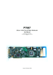
Fig. 2.1: MCS6 rear panel ............................................................................................................. 2-2
Fig. 2.2: MCS6 / MPANT startup screen....................................................................................... 2-3
Fig. 2.3: “MCS6 Settings” and “Inspect MCS6” window ............................................................... 2-4
Fig. 2.4: Axis Parameters window................................................................................................. 2-5
Fig. 2.5: Input Thresholds and ROI Presets window .................................................................... 2-5
Fig. 2.6: Spectrum of a 10 MHz clock signal................................................................................. 2-6
Fig. 2.7: Inputs set to 6 Input Channels and different Edges........................................................ 2-7
Fig. 2.8: Setup internal pulse train ................................................................................................ 2-8
Fig. 2.9: Spectrum of a N=7 pulse train ........................................................................................ 2-8
Fig. 2.10: MCS6 Settings – Acquisition Delay .............................................................................. 2-9
Fig. 2.11: Spectra with 96 ns acquisition delay........................................................................... 2-10
Fig. 2.12: Inputs setup for a pulse width measurement .............................................................. 2-11
Fig. 2.13: MCS6 Settings for a pulse width measurement.......................................................... 2-11
Fig. 2.14: MAP and Isometric View of a pulse width measurement ........................................... 2-12
Fig. 2.15: MAP View display options........................................................................................... 2-12
Fig. 2.16: Single Display Options................................................................................................ 2-13
Fig. 2.17: Single View of a pulse width measurement ................................................................ 2-13
Fig. 2.18: Two-dimensional position-sensitive detector .............................................................. 2-14
Fig. 2.19: Settings for acquisition with position-sensitive detector ............................................. 2-15
Fig. 2.20: Creating a dual-parameter spectra ............................................................................. 2-15
Fig. 2.21: View of dual-parameter spectra .................................................................................. 2-16
Fig. 2.22: Experimental setup .................................................................................................... 2-16
Fig. 2.23: Editing MCS6.INI ........................................................................................................ 2-17
Fig. 2.24: Testing and identifying three MCS6 modules ............................................................. 2-17
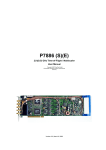
Fig. 3.1: MCS6 front panel ............................................................................................................ 3-1
Fig. 3.2: Thermal picture of the metal case................................................................................... 3-2
Fig. 3.3: START / STOP inputs..................................................................................................... 3-2
Fig. 3.4: MONITOR signal of a STOP input .................................................................................. 3-3
Fig. 3.5: Fast-NIM SYNC_1 output schematic .............................................................................. 3-5
Fig. 3.6: TAG input logic................................................................................................................ 3-5
Fig. 3.7: Schematic of FEATURE I/O connector........................................................................... 3-6
Fig. 3.8: TTL/LVDS TAG input schematic..................................................................................... 3-7
Fig. 4.1: Simplified timing diagram................................................................................................ 4-1
Fig. 4.2: FIFO concept .................................................................................................................. 4-3
Fig. 5.1: MCS6 Server Window..................................................................................................... 5-1
Fig. 5.2: MCS6 Ini File................................................................................................................... 5-2
Fig. 5.3: Data Operations dialog for MPA data (left) and selected spectra (right) ........................ 5-3
Fig. 5.4: Replay Settings dialog .................................................................................................... 5-4
Fig. 5.5: About MCS6 dialog box .................................................................................................. 5-4
Fig. 5.6: Settings dialog................................................................................................................. 5-5
Fig. 5.7: Inspect MCS6 dialog....................................................................................................... 5-7
Fig. 5.8: Input Thresholds dialog................................................................................................... 5-7
Fig. 5.9: Principle of "Software CFT" ............................................................................................ 5-9
Fig. 5.10: System Definition dialog box....................................................................................... 5-10
Fig. 5.11: System Definition dialog box, three MCS6 modules .................................................. 5-10
Fig. 5.12: Remote control dialog ................................................................................................. 5-11
Fig. 5.13: Dualparameter and Calculated spectra dialog box..................................................... 5-12
Fig. 5.14: Multi Display Setting ................................................................................................... 5-12
Fig. 5.15: Calculated Spectrum Setting ...................................................................................... 5-13
Fig. 5.16: Conditions ................................................................................................................... 5-14
Fig. 5.17: ROI Conditions dialog ................................................................................................. 5-14
Fig. 5.18: Combine Conditions dialog ......................................................................................... 5-15
Fig. 5.19: Test acquisition with calculated spectra ..................................................................... 5-15
Fig. 5.20: Defining two Spectra with Interleaved 50 psec time resolution .................................. 5-16
ComTec GmbH
V
Table of Figures
Fig. 5.21: How to adjust thresholds for Interleaved 50 psec time resolution .............................. 5-17
Fig. 5.22: Opening the DDE conversation with the MCS6 in LabVIEW ..................................... 5-26
Fig. 5.23: Executing a MCS6 command from a LabVIEW application ....................................... 5-27
Fig. 5.24: Getting the total number of data with LabVIEW ......................................................... 5-27
Fig. 5.25: Getting the data with LabVIEW................................................................................... 5-28
Fig. 5.26: Closing the DDE communication in LabVIEW ............................................................ 5-28
Fig. 5.27: Control Panel of the demo VI for LabVIEW ................................................................ 5-29
Fig. 6.1: MPANT main window...................................................................................................... 6-1
Fig. 6.2: MPANT Map and Isometric display................................................................................. 6-2
Fig. 6.3: File New Display dialog box............................................................................................ 6-3
Fig. 6.4: Print dialog box ............................................................................................................... 6-4
Fig. 6.5: Slice and rectangular ROI Editing dialog box ................................................................. 6-7
Fig. 6.6: Polygonal ROI Editing dialog box ................................................................................... 6-7
Fig. 6.7: Single Gaussian Peak Fit................................................................................................ 6-8
Fig. 6.8: Log file Options for the Single Gaussian Peak Fit .......................................................... 6-9
Fig. 6.9: Colors dialog box .......................................................................................................... 6-10
Fig. 6.10: Color Palette dialog box.............................................................................................. 6-10
Fig. 6.11: Single View dialog box................................................................................................ 6-11
Fig. 6.12: Custom-transformed spectra dialog............................................................................ 6-12
Fig. 6.13: MAP View dialog box .................................................................................................. 6-12
Fig. 6.14: Isometric View dialog box ........................................................................................... 6-13
Fig. 6.15: Axis Parameter dialog box .......................................................................................... 6-14
Fig. 6.16: Scale Parameters dialog box ...................................................................................... 6-15
Fig. 6.17: Calibration dialog box ................................................................................................. 6-16
Fig. 6.18: Comments dialog box ................................................................................................. 6-17
Fig. 6.19: Settings dialog box...................................................................................................... 6-17
Fig. 6.20: Data Operations dialog box ........................................................................................ 6-18
Fig. 6.21: System Definition dialog box....................................................................................... 6-18
Fig. 6.22: Spectra dialog box ...................................................................................................... 6-19
Fig. 6.23: Slice dialog box ........................................................................................................... 6-19
Fig. 6.24: Replay dialog box ....................................................................................................... 6-20
Fig. 6.25: Tool Bar dialog box ..................................................................................................... 6-20
Fig. 6.26: Function keys dialog box ............................................................................................ 6-21
Fig. 7.1: Autocorrelation software option ...................................................................................... 7-1
Fig. 8.1: 12mV and 8mV input pulses and cor. SYNC_1 MONITOR outputs............................... 8-6
Fig. 8.2: Spectrum of 12 mV pulses.............................................................................................. 8-6
Fig. 8.3: Spectrum of 8 mV pulses................................................................................................ 8-7
Fig. 8.4: Spectrum of 250 mV pulses............................................................................................ 8-7
Fig. 8.5: Peak Resolution at 1 ms after the Trigger ...................................................................... 8-8
Fig. 8.6: Peak Resolution at 100 ms after the Trigger .................................................................. 8-8
Fig. 8.7: Peak Resolution at 1,000 ms after the Trigger ............................................................... 8-8
Fig. 8.8: Pulse width measurement............................................................................................... 8-9
Fig. 8.9: SYNC_1 output signals: fall time, rise time, 200 MHz clock........................................... 8-9
Fig. 8.10: SYNC_2 output signals: rise time, fall time................................................................... 8-9
Fig. 8.11: SYNC_2 10 MHz clock output signal.......................................................................... 8-10
Fig. 8.12: SYNC_2 100 MHz clock output signal........................................................................ 8-10
Fig. 8.13: Power splitters for 50 psec option............................................................................... 8-12
ComTec GmbH
VI
WARNINGS
WARNINGS
The metal case of the MCS6 might be hot.
Beware of burning yourself!
The whole metal case works as a passive cooler for the device.
It can reach surface temperatures of well over 50°C.
The metal case of the MCS6 works as a passive cooler. Please provide ample airflow around the
device. Do not cover the case. Do not place it inside a closed cabinet etc.
Static electricity discharges can severely damage the MCS6. Use strict antistatic procedures
when connecting cables and during handling of the device.
Take care not to exceed the maximum input voltages as described in the technical data.
The START and STOP inputs are ultra high speed, high sensitivity inputs and thus, susceptible to
oscillation and noise pick-up. Take care to apply low impedance (≤ 50 Ω) source signals and well
shielded, 50 Ω coaxial cables.
ComTec GmbH
VII
Introduction
1.
Introduction
The Model MCS6 is a 100ps per time bin, multiple-event time digitizer (TDC). It can be used in
ultra-fast multi-scaler/TOF systems, in Time-of-Flight mass-spectrometry and time-resolved single
ion- or photon counting.
A unique feature is the MCS6’s capability to detect the rising and the falling edges
simultaneously. Thus, Time-over-Threshold (ToT) and Time-under-Threshold (TuT), i.e. pulsewidth measurements are easily accomplished.
Fig. 1.1: MCS6 transport case
Pulse-width evaluation with 100ps resolution enables the user to calculate the area, the pulseheight of the detector pulse but also if multiple events have occurred – multiple events have a
broader pulse width than single pulses.
A new genuine feature is the Constant-Fraction-Timing (CFT) mode. Some detectors will deliver
different height signals depending on the number of particles detected. To derive most accurate
timing information of the event a long known method is to use the constant farction timing. This
was previously only possible with analogue constant fraction timing discriminators. But these
have a main downfall, namely the acceptable data rate. With the MCS6’s capability of detecting
rising and falling edges simultaneously it is now possible to do that on a digital and thus, not(!)
bandwidth limited basis.
Also a new capability is to evaluate coincidental events at a resolution of 100 ps. Thus multidimensional spectra with 100 ps time resolution can be generated.
In standard operation a sweep is started by a user supplied start (trigger) pulse. Then subsequent
events detected at the STOP inputs are recorded, each in a specific time bin corresponding to the
time of arrival relative to the start pulse. Compared to non-multi-hit devices the MCS6 can
evaluate stop events at a rate of 10GHz state changes per second. In the pulse-width mode
ComTec GmbH
1-1
Introduction
pulses as narrow as 100ps can be evaluated at a pulse repetition rate of up to 5GHz. The MCS6
is designed with fully digital circuitry capable of accepting at least 65,000 events at peak (burst)
input rates of up to 10Gbit/s for each input.
The MCS6 has been optimized for the best pulse pair resolving while providing state-of-the-art
time resolution available in digital designs. Six built-in discriminators can be adjusted for a wide
range of input signal levels.
Sixteen TAG inputs allow for a wide range of spectra routing, multi detector experiments,
sequential acquisition etc.
An open-drain 'GO'-line (compatible to other products of FAST ComTec) allows for overall
experiment synchronization.
Two software configurable SYNC outputs provide synchronization and triggering of external
devices or experiment monitoring.
A versatile 8 bit digital I/O1 port may further satisfy your experimental needs.
The single sweep time range enables the user to take data of up to 20 days (54 bit setting) or
30 minutes (44 bit setting plus 16 TAG bits enabled) with a time resolution of 100 ps.
Via the 10 MHz reference I/O the already excellent stability of the internal oven controlled crystal
oscillator can be further improved by connecting an optional available high stability external
reference clock source such as a GPS or rubidium-disciplined oscillator.
The FIFO memory buffers enable to MCS6 to continuously transfer data rates of approximately
35 MByte/s to the connected computer. Available are FIFOs as large as 2 GB.
Selection of data width per event in steps of 16 bits (16, 32, 48 or 64 bits) allows for optimized
FIFO and USB bandwidth usage.
For experiments requiring repetitive sweeps the spectral data obtained from each sweep can be
summed in the PC enabling very high sweep repetition rates. In endless / wrap-around mode
sweep repetitions with zero end-of-sweep dead time can be accommodated.
The MCS6 is designed with “state-of-the-art” components, which offer excellent performance and
reliability. The high-performance hardware is matched by sophisticated WINDOWS™-based
software (delivered with each MCS6) providing a powerful graphical user interface for setup, data
transfer and spectral data display.
Some of MPANT´s features are high-resolution graphics displays with zoom, linear and
logarithmic (auto) scaling, grids, ROIs2, Gaussian fit, calibration using diverse formulas and
FWHM3 calculations. Macro generation using the powerful command language allows task
oriented batch processing and self-running experiments.
A DLL (Dynamic Link Library) is available for operation in a Laboratory Automation environment.
Drivers for LINUX are also available.
1 I/O: Input / Output
2 ROI: Region Of Interest
3 FWHM: Full Width at Half Maximum
ComTec GmbH
1-2
Installation Procedure
2.
Installation Procedure
2.1.
Hard- and Software Requirements
For operating the MCS6 you need a standard PC with USB 2.0 port and Microsoft Windows XP or
Vista. USB 1.0 ports do not work. The MCS6 works well using only one USB 2.0 port. The
maximum throughput is then 30 Mbyte/sec. This throughput can be somewhat increased by
using two USB ports. USB port 1 will then be used for controlling and parameter transfer, USB
port 2 will be used for data transfer only using two pipes acting interleaved in parallel switching 1
kbyte buffers between two different endpoints. The maximum throughput is then typically 35
Mbyte/sec, we have seen on one computer a record of about 40 Mbyte/sec.
The large 1 or 2 GB FIFO is able to buffer data recorded at 33 million events/sec. Of course it will
take some time after stopping an acquisition to empty a full FIFO, 2 Gbyte / 30Mb/sec is about a
minute. The filling status of the FIFO is shown in the software. There is also an indicator showing
if any data is lost. The fast FIFOs on each input channel can buffer data recorded with 10 GHz
without loss up to 6.5 mikrosec. See chapter 4.3 in this manual.
We do not expect any problems with host compatibility as we do not use something else than any
USB hard disk or memory stick. Of course it is necessary that the PC has a true USB 2.0 port.
Older PC's that do not have USB 2.0 on the motherboard can use a PCI card providing USB 2.0
ports. We have no good experience with such PCI cards, the throughput will be much lower,
typically only 15..20 Mbyte/sec, and some cards may not work at all. So we recommend a PC
with true USB 2.0 ports on the motherboard, as is now standard even for laptops.
First check you have all shipped equipment available:
•
Transport case (ref. Fig. 1.1)
•
MCS6 module
•
Power supply module 100…240 VAC / 12 VDC
•
Power line cord
•
(6x) SMA – BNC cable, RG316, 2 m
•
(2x) USB 2.0 (A/B) cable, 3 m
•
User manual
•
CD with operating software
•
USB stick with operating software
NOTE:
Please install the software before connecting the MCS6 to your computer.
2.2.
Software Installation
To install the MCS6 software on your hard disk insert the MCS6 installation medium (CD or USBStick) and start the installation program by double clicking from the explorer
SETUP
If you connect the USB cable, the device manager will recognize the new hardware, and will ask
for a driver. Please insert then the installation disk and specify the WDMDRIV\XP or
WDMDRIV\Vista directory on the installation medium as the driver location, corresponding to your
Windows version.
ComTec GmbH
2-1
Installation Procedure
A directory called C:\MCS6 is created on the hard disk and all MCS6 and MPANT files are
transferred to this directory. Drive C: is taken as default drive and \MCS6 as default directory. It is
not mandatory that the MCS6 operating software is located in this directory. You may specify
another directory during the installation or may copy the files later to any other directory.
The Setup program has installed a shortcut on the desktop. The icon starts directly the
MCS6.EXE. The server program will automatically call the MPANT.EXE program when it is
executed. The MCS6 Server program controls the MCS6 module but provides no graphics
display capability by itself. By using the MPANT program, the user has complete control of the
MCS6 along with the MPANT display capabilities.
To run the MCS6 software, simply double click on the “MCS6 Server Program“ icon. To close it,
close the MCS6 server in the Taskbar.
2.3.
Hardware Installation
Installation of the MCS6 is as easy as connecting a cable. Connect the power supply to the “+12V
Supply” connector and a USB 2.0 cable to the “USB 1” port. At the host computer plug in the USB
cable into a high-speed capable USB 2.0 port. Since USB is a hot-pluggable interface the
sequence of applying power and connecting the USB port is not important.
NOTE:
At the host computer a high-speed (480 Mbit/s4) capable USB 2.0 interface must be used.
When power is applied the “POWER ON” LED on the front of the MCS6 should be lit and a
second later “POWER GOOD” as well.
Fig. 2.1: MCS6 rear panel
If you intend to use 2 USB ports for higher data transfer rates also connect “USB 2”.
IMPORTANT:
All setup and control data exchange is handled over “USB 1”. Thus, “USB 1” must always be
connected to the host computer.
4 The USB 2.0 specification includes low-speed (1.5 Mbit/s), full-speed (12 Mbit/s) and high-speed (480 Mbit/s) signaling rates
ComTec GmbH
2-2
Installation Procedure
When the software and driver are already installed the computer will detect the MCS6
automatically as soon as it is connected.
2.4.
Getting Started
The Model MCS6 has built-in signal generators that enable you to get familiar with the device
usage without any external signal sources.
There are 2 possible ways to get measurements running without external signals:
1) an internal pulse generator can be internally fed to all START / STOP inputs
2) the SYNC_1 output can be connected to inputs using cables and maybe a power splitter
2.4.1.
st
1 Basic Measurements
To ease getting familiar with the use of the MCS6 we will now setup a first basic measurement.
Thanks to the built-in signal generator and the “internal pulser” mode no external signals or
additional connections are needed.
Start the MCS6 software by double clicking the corresponding icon. This will automatically start
the MPANT program. On startup the MCS6 server is iconized and one does not have to worry
about it since all hardware settings are as well accessible from the MPANT program which
actually is the graphical user interface and which will now appear on the screen (ref. Fig. 2.2).
Fig. 2.2: MCS6 / MPANT startup screen
Now we first have to setup the MCS6. What we will want to do is to setup the system such that
we use the internal pulser and acquire a spectrum of 4096 time bins using input channel STOP 1.
Click on Options – Range, Preset… or
to find the MCS6 Settings window pop up. Set the
Range to 4096 time bins (Bin width = 1), which corresponds to a time range of 409.5 ns. Enable
Sweep preset and set it to e.g. 20,000,000. Verify that Timepreset is not checked (ref. Fig. 2.3).
Now click on Inspect… and you will see the Inspect MCS6 window pop up. Enable the internal
pulser and select a signal of 10 MHz (ref. Fig. 2.3).
ComTec GmbH
2-3
Installation Procedure
Fig. 2.3: “MCS6 Settings” and “Inspect MCS6” window
Now click on Inputs…. Select CH 1 and deselect all other input channels. Check that Falling Edge
is selected for both CH 6 / Start and CH 1 (ref. Fig. 2.5). Do not worry about the threshold levels
since we use the internal pulser, which does bypass the input discriminators. Click OK.
You are back in the Settings window. Also click OK here. Now we enable a grid selecting Options
– Axis… or
and ticking the grid enables (ref. Fig. 2.4).
Now start the acquisition by a mouse click on Action – Start or the start button . You will see a
spectrum growing that is comprised of needles separated by 1000 channels or 100ns, which
corresponds to the selected 10 MHz pulser signal. After a while the sweep preset of 20,000,000
will be reached and acquisition is stopped (ref. Fig. 2.6).
You might want to zoom into a specific peak by holding the right mouse button and drawing up a
window inside the spectrum. Then click on Region – Zoom or . With the left mouse button you
can move a cursor round the spectrum giving information on its time position and counts in the
corresponding bin. Play around with zooming in and out, toggling lin/log scale and Gaussian fit.
ComTec GmbH
2-4
Installation Procedure
Fig. 2.4: Axis Parameters window
Fig. 2.5: Input Thresholds and ROI Presets window
ComTec GmbH
2-5
Installation Procedure
Fig. 2.6: Spectrum of a 10 MHz clock signal
ComTec GmbH
2-6
Installation Procedure
2.4.2.
nd
2
Introductional Measurement
So far so good. Now lets plunge a little deeper into the capabilities of the MCS6 by using several
channels measuring different edges of a more complex input waveform. We use a built-in pulsetrain generator that delivers 10 ns wide, negative-going pulses that are separated by 30 ns and
repeated N times (with N selectable from 1 to 255). The whole pulse-train is restarted every
10.24 µs.
Lets enable all 5 STOP channels and the sampling of the START input as well (ref. Fig. 2.7).
Thus, after a sweep is triggered the subsequent events into the START channel are acquired as
th
well. Using this feature the START input works like a 6 input channel. As can be seen in Fig. 2.7
we set the edge detection of CH 6 / START, CH 1 and CH 4 to ‘Falling’. Channel 2 is set to
‘Rising’ and the channels 3 and 5 to ‘Both Edges’. Triggering is done with the falling edge of the
START input signal (‘Start with rising edge’ is not checked). The threshold voltages can still be
ignored due to the use of the internal pulser.
Fig. 2.7: Inputs set to 6 Input Channels and different Edges
Now let’s set the internal pulser to pulse train mode and the number of subsequent pulses to
seven (ref. Fig. 2.8).
Now that you have set the MCS6 to the use of 6 input channels the MPANT program will show 6
client windows, one for each input channel. The window ‘A6’ shows the START input, ‘A1’ to ‘A5’
the STOP inputs 1 to 5.
ComTec GmbH
2-7
Installation Procedure
Fig. 2.8: Setup internal pulse train
When you start the acquisition now 6 spectra like in Fig. 2.9 will build up. To indicate the
correlation of input signal edges to the peaks in the spectra the selected pulse train is drafted in
the picture. You can easily see the signal period of 40 ns and that the sweeps were triggered on
the falling edge etc. The pulse width of 10 ns can be very well seen in the spectra with both
edges enabled.
Fig. 2.9: Spectrum of a N=7 pulse train
Now we will introduce another feature of the MCS6: the acquisition delay. This is very useful
when we want to discard events in a specified time occurring directly after the trigger pulse. In
some experiments this can dramatically reduce the measured event rate. In our example we will
ComTec GmbH
2-8
Installation Procedure
want to acquire data only beginning 96 ns (settable in steps of 6.4 ns only) after the START
event. Go to the MCS6 Settings window again and insert ‘96’ in the Acq. Delay field (ref. Fig.
2.10). With all other settings left as before we will expect the first 960 time bins of the above
spectra to “disappear” i.e. the spectra being shifted left by 960 bins or 96 ns.
Fig. 2.10: MCS6 Settings – Acquisition Delay
Start acquisition and compare the delayed spectra data (ref. Fig. 2.11) with the above spectra
that began instantly with the START pulse. Referring the input channel STOP 1 (A1) spectrum
you see that the first 3 peaks at position 0, 400 and 800 have disappeared. The first peak in the
new spectrum is at channel 240 corresponding to time bin 1200 in Fig. 2.9. And, as expected,
only 4 peaks are left compared to the 7 peaks before.
ComTec GmbH
2-9
Installation Procedure
Fig. 2.11: Spectra with 96 ns acquisition delay
2.4.3.
Pulse-Width Measurement
Now lets see how the pulse width measurement mode works and how the different graphical
display modes can be used.
Go to the ‘Inputs Thresholds and ROI Presets’ window again and enable channel 1 with ‘Both
Edges’ to be sampled (ref. Fig. 2.12). For ‘Pulse width mode’ select ‘Under threshold’. This
implies that a pulse is expected to start with a falling edge. Remember the internal pulser that we
are using delivers negative going pulses of 10 ns every 40 ns. And, we start the sweeps with the
first falling edge (‘Start with rising edge’ is not checked).
ComTec GmbH
2-10
Installation Procedure
Fig. 2.12: Inputs setup for a pulse width measurement
Back in the ‘MCS6 Settings’ window make sure that ‘Pulse width’ is checked with an ‘y-Range’ of
2 for the falling and the rising edge (ref. Fig. 2.13). The acquisition delay should be ‘0’.
Fig. 2.13: MCS6 Settings for a pulse width measurement
The display will switch into a ‘MAP View’ mode, i.e. you are looking from a birds view onto two
spectra – the lower for the falling edges and the upper spectrum for the rising edges.
ComTec GmbH
2-11
Installation Procedure
Start the acquisition and you will see peaks grow their height indicated by color-coding. With
you can toggle between the 2- and a 3-dimensional view.
Fig. 2.14: MAP and Isometric View of a pulse width measurement
Go back to the 2-dimensional MAP view and then, click on Options – Display… and select
‘>> Overlapped’ (Fig. 2.15).
Fig. 2.15: MAP View display options
The spectrum display changes to a 2-dimensional spectrum with rising and falling edges that are
drawn overlapped (ref. Fig. 2.17). With the Display Options window you can choose which edges
should be in the fore- and background (Fig. 2.16). Always the foreground spectrum can be
measured using a mouse cursor. By pressing the left mouse button you can move the cursor and
see the corresponding data of time bin and counts below the spectrum.
ComTec GmbH
2-12
Installation Procedure
Fig. 2.16: Single Display Options
Fig. 2.17: Single View of a pulse width measurement
ComTec GmbH
2-13
Installation Procedure
2.4.4.
Using a two-dimensional position sensitive detector
Position-sensitive detectors often work by a delay-line readout. An example is shown in Fig. 2.18.
To get a two-dimensional histogram usually at least two TDC's (time-to-digital converter) and a
multiparameter data acquisition system is needed, for example the FAST ComTec 7072T and
MPA-3. Now let's see how the MCS6 can be used to do the same.
Fig. 2.18: Two-dimensional position-sensitive detector
Let's assume that the detector has in both x- and y- direction 150 wires and a delay-line of 2.7 ns
between each wire, i.e. a total delay of 405 nsec. The MCS6 offers 100 psec time resolution, i.e.
4096 time bins would be the maximum possible range that could be used. For the 150 wires a
resolution of 1k x 1k is certainly good enough, so a range of 1024 and a bin width of 4 is
reasonable. A common trigger signal must be connected to the "START" input, the x-stop signal
to the "STOP1" input, the y-stop signal to "STOP2".
Click the "Range, Preset" toolbar icon.
See Fig. 2.19 for possible settings. Set the bin width to 4. Make sure that the checkbox
"Sweepcounter in data not needed" is not checked. The sweep counter actually is necessary to
enable the unique assignment of events from separated input channels to the same trigger event.
Click the "Inputs" button to open the dialog for "Input Thresholds and ROI Presets"
The input channels CH1 and CH2 must be enabled, and suited thresholds for the signals must be
set. In principle both edges of the signals could be evaluated and a "software constant fraction"
method could be used to get an improved time resolution (see Fig. 5.9).
ComTec GmbH
2-14
Installation Procedure
Fig. 2.19: Settings for acquisition with position-sensitive detector
Now a two-dimensional histogram for the two parameters must be defined. Open the "Spectra"
dialog by clicking the corresponding toolbar icon.
Click "Add Multi" to define a dual-parameter spectra. In the "Multi Display Setting" dialog select
CHN1 for the x-parameter and CHN2 for the y-parameter. Select 1024 for both Ranges.
Fig. 2.20: Creating a dual-parameter spectra
Fig. 2.21 shows a view of such a dual-parameter spectra in the MCS6 software, Fig. 2.22 a photo
of the corresponding experimental setup. An example spectra named "tongs.mpa" can be found
in the sample data supplied with the software.
Instead of using only one signal for each position coordinate, one could read out the detector
from both sides and get two signals for each direction, i.e. in total one trigger signal and four stop
signals. The difference of the time from the left and right side gives an improved position
ComTec GmbH
2-15
Installation Procedure
parameter, and one could calculate in addition the sum of the signals from both ends and set a
condition on events inside a ROI (Region of Interest) around the sum peak in the sum spectra. All
this can be done with the MCS6, example settings are described in chapter 5-11.
Fig. 2.21: View of dual-parameter spectra
Fig. 2.22: Experimental setup
ComTec GmbH
2-16
Installation Procedure
2.5.
Installing more than one MCS6 modules
The software is able to operate up to three MCS6 modules with a single computer (if you need
more, contact us and we will expand the software). Each may be connected either by one or two
USB cables. When using only one USB line per MCS6 module, it is simple: just connect them at
USB1, switch on the power, and install the driver when you are prompted. When starting the
software, you will be asked to edit the MCS6.INI file as more than one MCS6 modules are found,
and the notepad editor will be automatically started with MCS6.INI loaded. Edit the line
"devices=1" accordingly and save the file.
Fig. 2.23: Editing MCS6.INI
That is all you have to do, next time when you start the software all modules will be found and
can be operated.
Fig. 2.24: Testing and identifying three MCS6 modules
ComTec GmbH
2-17
Installation Procedure
When connecting 2 USB cables to one or more MCS6 modules, it is more complicated. The
software cannot automatically identify which USB2 and USB1 ports belong together. So it is
recommended to use the built-in test pulser and set different signals for each module, for
example a pulse train with 5 pulses for module A, 2 pulses for module B and three pulses for
module C. The data are transfered via the USB2 line, so the pattern may be exchanged between
different modules to what you expect. In this case exchange the corresponding cables connected
at USB2 and restart the software, until you get a picture as shown in Fig. 2.24.
To get a quick identification which physical MCS6 module belongs to a module shown in the
software, you can use the "ID" button in the status window shown at the left beside the spectra in
MPANT. The LED's at the front panel will blink and the internal serial number will be shown
beside the ID button.
ComTec GmbH
2-18
Hardware Description
3.
Hardware Description
3.1.
Overview
The MCS6 is a USB 2.0 device with two high-speed USB 2.0 ports. It is able to measure multiple
events in up to 6 input channels at a time resolution of 100 ps. The logic is capable to
accommodate an incredible burst edge rate of 10 GHz. Such a burst can last for up to 6.5 µs
before any event might be lost. And that for each input channel independently. No dead time
between the time bins and secure prevention of double counting is established by the
sophisticated input logic.
A unique feature is the MCS6’s capability to measure falling and rising edges simultaneously.
Thus, Time-over-Threshold or pulse width measurements are easily accomplished.
Fig. 3.1: MCS6 front panel
Each input channel has its own onboard discriminator with individually adjustable threshold
levels. Adjustment is supported by a monitor capability of each discriminated signal.
Besides, two SYNC outputs with a large variety of output signal options (all software selectable)
and the ‘GO’-line (compatible with other FAST ComTec products) allow for easy synchronization
or triggering of other measurement equipment.
Furthermore a very versatile 8 bit digital I/O port allows for a whole bunch of experimental control,
monitoring or whatsoever tasks.
Moreover the 16-bit TAG input allows more multi-detector configurations, sequential data
acquisition etc.
Also improved are more built-in test capabilities than ever before. An internal pulse generator
allows for hardware tests and also to get familiar with all of the operation modes without the need
to setup external hardware.
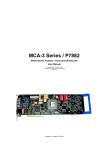
And there is the optional 2 GB large FIFO that extends the onboard storage capabilities.
The MCS6 contains many very high-speed logic circuits, which usually need large supply currents
and thus, produce high thermal power loss. To dissipate this thermal energy the complete metal
case is used for passive cooling. This improves reliability since no mechanically moving devices
like fans are involved. The downside is that the case can get quite warm or even hot. Refer Fig.
3.2, which is taken in a standard laboratory environment with the MCS6 placed on a table and no
other devices nearby. The crosses indicate local temperatures. The upper left cross shows the
ambient temperature of 22.9°C. The middle left cross indicates 45.3°C. With increasing ambient
temperature the maximum case temperature will increase as well. And also reduced airflow will
result in higher case temperature. In the software a temperature monitor feature is provided that
shows the internal FPGA and PCB temperatures.
ComTec GmbH
3-1
Hardware Description
Fig. 3.2: Thermal picture of the metal case
WARNING:
The metal case can get very warm or even hot. Beware of burning yourself.
IMPORTANT NOTE:
Provide ample airflow around the device for proper cooling. Do not cover the case. Do not place it
inside closed cabinets etc.
3.2.
START / STOP Inputs
The START (trigger) and STOP 1…5 (event) inputs are SMA types located on the front panel.
The input impedance is 50 Ω to ground. The inputs are edge sensitive with software selectable
rising, falling or even both edges. The threshold is software tunable in a range of ±1.5 V. In most
cases the threshold should be set right in the middle of the input pulse amplitude.
The sensitivity of these inputs is better than 10 mV. Please refer chapter 8.3.1 for example scope
pictures and related spectra. .
Fig. 3.3: START / STOP inputs
For input protection low capacity (approx. 1pF per diode) clamp diodes are provided. The clamp
voltages follow the threshold level by ±1.5 V. Thus, the input voltage level should not exceed the
threshold level by ±1.5 V or the diodes will become forward biased.
ComTec GmbH
3-2
Hardware Description
WARNING:
Take care not to exceed the maximum input voltages as described in the technical data.
Discriminator Propagation Delay Dispersion
The input discriminators propagation delay varies slightly with input overdrive voltage and slew
rate. When overdrive varies from 10 mV to 500 mV and slew rate varies from 1 V/ns to 10 V/ns
the delay can vary for up to 25 ps, which is ¼ of the bin width. This specification applies for both
positive and negative going signals.
For overdrive voltages above 200 mV the delay variation due to overdrive dispersion is mostly
negligible.
Monitoring the Inputs
To ease the adjustment of the threshold levels the discriminator outputs are sampled at a
frequency of 312.5 MHz cor. 3.2 ns and can be output on the SYNC outputs. Preferable SYNC_1
should be used as it is a fast-NIM output and provides best speed and edge rates.
Due to the 3.2 ns sampling the delay of the monitor signal relative to the input pulse will vary by
3.2 ns as well. The minimum output pulse width will be 3.2 ns and thus, even for very narrow
input pulses only 300…500 MHz scopes are necessary to see the monitor signals. Be aware that
for pulses smaller than 3.2 ns the detection probability will be below ‘1’ i.e. “pulse width [ns]/ 3.2”.
NOTE: this is only true for the monitor output and not for the spectrum acquisition. For spectrum
acquisition the pulses can be as narrow as 100 ps and still are 100% detected.
5
Fig. 3.4: MONITOR signal of a STOP input
Input Slew Rate Requirements
Due to the high bandwidth nature of the input discriminators, a minimum slew rate of the input
signal should be met to ensure proper switching and that the input does not oscillate when the
input signal crosses the threshold level. A minimum slew rate of 50 V/µs should ensure clean
signal transition.
For other reasons the slew rate should be high as well. The extremely high bandwidth of the
device means that broadband noise can have significant impact on the detection accuracy when
the slew rate is low. The input termination resistors generate 120 µV of thermal noise over the
discriminator’s bandwidth at room temperature. With a slew rate of 50 V/µs, the inputs will be
5 This scope picture is taken with a 2 GS/s, 500 MHz bandwidth digital scope
ComTec GmbH
3-3
Hardware Description
inside the noise band for over 2 ps. In reality the temperature will be higher and thus the thermal
noise.
3.3.
SYNC Outputs
The SYNC outputs provide a large variety of output signals for a lot of synchronizing, triggering,
monitoring or whatever application. The selectable output signals are as follows:
• 0
static "0"
• 10 MHz
10 MHz reference clock
• 78.125 MHz
10 GHz free running sampling clock / 128
• 100.000 MHz
100 MHz free running clock
• 156.250 MHz
10 GHz free running sampling clock / 64
• 200.000 MHz
200 MHz free running clock
• 312.500 MHz
10 GHz free running sampling clock / 32
• START
monitor of the discriminated START input sampled at 312.5 MHz
• STOP 1
monitor of the discriminated STOP 1 input sampled at 312.5 MHz
• STOP 2
monitor of the discriminated STOP 2 input sampled at 312.5 MHz
• STOP 3
monitor of the discriminated STOP 3 input sampled at 312.5 MHz
• STOP 4
monitor of the discriminated STOP 4 input sampled at 312.5 MHz
• STOP 5
monitor of the discriminated STOP 5 input sampled at 312.5 MHz
• GO
GO-line state
• START-OF-SWEEP
6.4 ns pulse at the beginning of a new sweep
• ARMED
ready for START
• SYS_ON
acquisition ON
• WINDOW
measurement time window
• HOLD_OFF
active HOLD-OFF time
• EOS_DEADTIME
active from the end of a sweep till re-arm
• TIME[0]
6.4ns = 2 x 6.4 ns periodic timer signal active only when sampling
• TIME[1]
12.8ns = 2 x 6.4 ns periodic timer signal active only when sampling
…
0
1
…
31
• TIME[31]
13.7s = 2
• SWEEP[0]
bit 0 of the sweep counter
• SWEEP[1]
bit 1 of the sweep counter
…
• SWEEP[11]
x 6.4 ns periodic timer signal active only when sampling
…
bit 11 of the sweep counter
All these signals may be output on the fast-NIM SYNC_1 output on the front panel and on the
TTL SYNC_2 output on the FEATURE connector as well. They can also be inverted.
The sweep counter is incremented when a new sweep is started / triggered.
ComTec GmbH
3-4
Hardware Description
Fig. 3.5: Fast-NIM SYNC_1 output schematic
The fast-NIM SYNC_1 output is a current mode output and supplies standard fast-NIM (0...-0.8 V
/ 16 mA) signals into an external 50 Ω load. The output impedance is 50 Ω. For fast-NIM signals a
logic ‘TRUE’ corresponds to a low voltage (-0.7 V), e.g. while a sweep is running ‘ON’ will result in
–0.7 V (=’TRUE) output. You can switch to negative logic by selecting ‘inverted’ in the
corresponding settings.
3.4.
TAG Inputs
A unique feature of the MCS6 is a 16-bit TTL/LVDS TAG input with a time resolution of 6.4 ns.
As can be seen from the simplified logic diagram in Fig. 3.6 the TTL ENABLE must be connected
to +5 V when the TTL TAG inputs shall be used. A short between pin 37 and pin 19 on the 37-pin
D-SUB connector will be sufficient.
TTL
ENABLE
TO OTHER
TAG INPUTS
PULLDOWN
32 k Ω
TTL ENABLE
TAG_IN(x)
100 Ω
+5V
TTL TAG
INPUT(x)
LVDS TAG
INPUT(x)
7V
PULLDOWN
110 Ω
Fig. 3.6: TAG input logic
NOTE:
For usage of the LVDS TAG input mode please contact factory for details.
For details on the pinning of the connectors please refer Fig. 3.8.
When in use the TAG inputs are stored with each detected event at a resolution of 6.4 ns.
Since it might mostly take some time to derive the proper TAG signals from the experimental
setup (e.g. due to further external logic delays etc.) the MCS6 provides a software settable input
delay to the START and STOP inputs. This can be set in 15 steps of 3.2 ns each in a range of
0…48 ns. Thus adjustment of the arrival times of TAG to STOP signals was never that easy.
ComTec GmbH
3-5
Hardware Description
3.5.
‘GO’-Line
The ‘GO’ line is a system-wide open-drain wired-AND signal that can start and stop a
measurement. This line is available on the FEATURE connector and on the specific BNC
connector on the rear panel.
The ‘GO’ line may be enabled, disabled, set and reset by the software. The system-wide opendrain ‘GO’ line enables any connected device to enable and to stop all participating measurement
equipment simultaneously. This allows for easy synchronization of electronic devices previously
often not possible.
When watching of the ‘GO’ line is enabled for the MCS6, a low voltage will halt the measurement.
When output to the ‘GO’ line is enabled, starting a measurement (i.e. the MCS6 is armed) will
release the ‘GO’ line (high impedance output) whereas a halt of the measurement will pull-down
the ‘GO’ line to a low state. Since it is an open-drain output wired-AND connection with other
devices is possible. Also refer Fig. 3.7.
The ‘GO’ line is available on most of the other FAST ComTec products as well.
3.6.
FEATURE (Multi-) I/O Connector
A very versatile 8 bit digital I/O port is implemented on the 15-pin high-density female D-SUB
connector. The pull-up and series resistors (ref. Fig. 3.7) of the digital I/O ports are socket
mounted and thus, can be easily adapted to specific needs.
This I/O port is fully software controllable and each single (1-bit) port is individually configurable.
Each individual port can be configured as input only (tri-stated output) or open-drain (pull-up)
output with read back capability. Wired-OR/AND connections are also feasible.
It might be used for external alert signals, sample changer control, status inputs / outputs etc.
Fig. 3.7: Schematic of FEATURE I/O connector
NOTE:
Please contact factory if changes to the resistors are needed.
Also on the FEATURE connector there is the TTL SYNC_2 output.
Furthermore an analog output is provided. The output voltage is software controllable in a range
of 0…+2.5 V with a 14 bit or 0.15 mV resolution.
ComTec GmbH
3-6
Hardware Description
Fig. 3.8: TTL/LVDS TAG input schematic
ComTec GmbH
3-7
Hardware Description
3.7.
Time Base / Reference Clock
To derive the outstanding temperature and long-term stability the MCS6 is equipped with an onboard ovenized crystal oscillator (OCXO). This OCXO stabilizes the 10 GHz PLL (phase locked
loop) synthesizer that clocks the sampling circuitry.
The reference is a 10 MHz clock. Either the internal (on-board) or an external reference is
software selectable, see section 5.1.1. See in 8.2.3 for the signal impedance and amplitude.
For highest stability and accuracy Rubidium disciplined oscillators or GPS controlled clock
generators are available.
ComTec GmbH
3-8
Functional Description
4.
Functional Description
4.1.
Introduction
The MCS6 measures the arrival time of STOP input events relative to a previous START signal.
The resolution or time bin width is 100 ps. The full dynamic range is 54 bits which results in the
incredible maximum sweep time of 20.84 days. 32 bits [6…37] of the timer are also accessible via
the SYNC outputs (TIME[0…31], ref. Chapter 3.3). The measured data is transferred into the
computer in list-mode, i.e. as they are acquired per each input channel.
A unique feature of the MCS6 is that the START channel can be sampled as well and thus can be
used as a sixth input channel.
Since the time base for all 6 inputs is the very same and since each data transferred into the PC
contains the channel number and a long time information relative to a common start (even
software start) for the first time correlation's between several input channels can be acquired with
one single instrument. Time differences or correlation's between specific events in up to 6
different channels can be measured. And this always at the full 100 ps resolution even for long
time periods.
4.2.
Modes of Operation
4.2.1.
Stop-After-Sweep Mode
This might be the mode many have used before with single channel instruments.
When the MCS6 is armed it waits for a START input signal. When one occurs the sweep is
started / triggered, meaning the time starts to count. Now the arrival times of the STOP input
signals relative to the start are acquired on all channels that are enabled. A STOP event can be
either a falling or a rising edge or both. Even further signals into the START input can be
acquired. Since the type of edge is detected and marked in the acquired data even Time-overThreshold or pulse width measurements can be accomplished.
An acquisition delay time might be selected in steps of 6.4 ns to accept only STOP events that
arrive after the selected delay.
Fig. 4.1: Simplified timing diagram
When the selected measurement time range – selectable in steps of 6.4 ns - has elapsed the
sweep and so the data acquisition ends. After a short (96 ns) end-of-sweep dead time the MCS6
is ready for a new start and will begin a new sweep as soon as the next START event occurs.
ComTec GmbH
4-1
Functional Description
To reduce the overall average data rate a HOLD OFF time might be selected – as well in steps of
6.4 ns - that allows a new start only after this additional time has elapsed after the end of the
sweep.
Acquisition delay, time range and hold-off are 48 bit values in 6.4 ns units each.
48
Acq.Delay + TimeRange + Hold-Off ≤ 2 x 6.4 ns = 20 days max.
Since the time window in which events are actually acquired is programmable in such a wide
range it is possible to count stop events at very high input rates even at late arrival times. This is
due to the data reduction executed. The fact is that all events that occur outside the programmed
time range window are discarded.
Example 1:
Average STOP data rate of 100 MHz. Interesting time window is 1 µs at 1 ms after the START /
TRIGGER signal:
In a time range of 1 ms the 100 MHz input rate would result in 100,000 STOP events which would
cause data loss due to filled FIFO's. When programming an acquisition offset of 1 ms and a 1 µs
measurement time window the resulting number of events per sweep is only 100. Thus, no data
loss at all will occur. And even with highest speed sweep repetition rates an average data rate of
only some 1000 sweeps/sec x 100 events/sweep = 100,000 events/sec has to be stored.
Additionally a trigger hold-off time, also programmable in increments of 6.4 ns, can be selected to
further reduce the average data rate by accepting only a new start / trigger after this additional
time has elapsed.
Example 2:
Average number of STOP events per sweep is 1,000. Say your computer allows an average
transfer rate over the USB of 10 Mevents/s a maximum of 10MHz / 1000 = 10kHz sweep
repetition rate can be accepted. With a sweep length of e.g. <5 µs and start signals every 5 µs
the average data rate would be 200 MHz. A trigger hold off after every sweep of 95 µs will reduce
the start rate to 10 kHz and thus the average count rate to 10kHz x 1,000 = 10MHz.
Sweep counter
A presettable 48-bit sweep counter is incremented at every start of a sweep. In fact the sweep
counter counts the real start of a new sweep rather than the completion of the sweeps. When a
preset is enabled and the preselected number of sweeps has occurred any further start of a
sweep is prohibited.
The lowest 12 bits of the sweep counter may be output and watched on the SYNC outputs. They
are particularly useful when some experiment should be periodically changed after a fixed
number of sweeps.
4.2.2.
Endless Mode
In the endless mode data acquisition is started only once, e.g. by a software start i.e.
asynchronously to the rest of the experiment. Then all arriving events are recorded and stored
with an absolute time relative only to the initial start. Since the dynamic range is up to 54 bit or
20 days the available absolute time range will be sufficient for every imaginable experiment.
4.2.3.
Tagged Spectra Acquisition
16 TAG inputs allow for sequenced spectra acquisition, multi detector configurations etc. The
16 Tag's are sampled synchronously to the START / STOP inputs. The time resolution is 6.4 ns.
E.g. in a multi detector experiment it is feasible to measure which detector (even if more than 5)
has fired and still maintain the incredible 100 ps bin width. This allows also for ultra fast
coincidence measurements with very little external logic required.
ComTec GmbH
4-2
Functional Description
In most cases the arrival time of the TAG signals relative to the corresponding STOP signals will
be late. To ease the adjustment of the arrival time between TAG and STOP signals a digital
selectable additional delay to the START /STOP signals is provided. This can delay those signals
in steps of 3.2 ns in a range of 0 to 48 ns. Thus, normally no external delay lines will be needed.
In case of using the TAG bits part of the upper 32 bits of the 64 bit data word are replaced by the
Tag's.
4.3.
FIFO Concept
A multi-stage FIFO concept is used to optimize for the two main difficulties of those data
acquisition systems. On the one hand ultra high burst count rates (here 10 Gevents/s) should be
acceptable for a period of time as long as possible.
Fig. 4.2: FIFO concept
In the case of the MCS6 each individual START / STOP input has its own 6.4 ns x 1024 FIFO.
These are able to store burst rates of as high as 10 G edge events per second for up to 6.5 µs
before any event might be lost. Each FIFO word is comprised of the complete event structure in a
6.4 ns period. It is worth noting that these ultra fast FIFO's are really independent for each
channel.
On the other hand a high average count rate must be stored without loss of events. The decoding
and binary time coding of the raw data as buffered in the first FIFO stage is accomplished at a
rate of over 33 MHz. Since the bandwidth of the USB 2.0 transmission is limited to something like
35 MB/s a large second FIFO is provided that is able to store a high number of data.
The optional up to 2 GB large DDR2 FIFO is designed to be used in an optimized way depending
on the number of bytes that is transferred for each single event. I.e. for 64 bit = 8 byte data words
up to 2 GB / 8 = 256 Mevents can be buffered. The same is true for 48 bit = 6 byte words. For
32 bit = 4 byte data up to 512 Mevents, for 16 bit = 2 byte data up to 1 Gevents can be stored in a
2 GB DDR2 module.
ComTec GmbH
4-3
Software Description
5.
Software Description
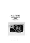
The window of the MCS6 server program is shown here. It enables the full control of the MCS6 to
perform measurements and save data. This program has no own spectra display, but it provides via a DLL (“dynamic link library“) - access to all functions, parameters and data. The server can
be completely controlled from the MPANT software that provides all necessary graphic displays.
Fig. 5.1: MCS6 Server Window
5.1.
Server functions
To start the software, just double click a shortcut icon linking to the server program. The server
program performs a test whether the hardware works well on this computer, then starts MPANT
and gets iconized. Usually you will control everything from MPANT, but it is possible to work with
the server alone and independently from MPANT.
5.1.1.
Initialization files
At program start the configuration files MCS6.INI and MCS6A.SET are loaded.
ComTec GmbH
5-1
Software Description
Fig. 5.2: MCS6 Ini File
Parameters that can be set by editing the MCS6.INI file are the update rate in msec for the
refresh of the status, and it can be specified whether 2GB or 1GB RAM is built in. Set
DDR_2GB=0 for 1GB.
External clock: If you have a good external 10 MHz reference signal, for example a Rubidium or
GPS clock, you can use it the following way:
Change the MCS6.INI file and insert a line
extclk=1
After power up always the internal clock is used, so you should not yet connect the external clock
signal. Start the software. You will be prompted by a Messagebox to connect the external 10 MHz
signal to the BNC connector labeled "10 MHz" at the back side. If you later exit and restart the
software, let it connected. But after power down please disconnect it. When using the internal
clock the same connector outputs the internal 10 MHz signal.
The file MCS6A.SET contains the default settings. It is not necessary to edit this file since it is
saved automatically. Instead of this .SET file any other setup file can be used if its name without
the appendix ‘A.SET’ is used as command line parameter (e.g. MCS6 TEST to load
TESTA.SET).
5.1.2.
Action menu
The server program normally is shown as an icon in the taskbar. After clicking the icon it is
opened to show the status window. Using the „Start“ menu item from the action menu a
measurement can be started. In the status window every second the acquired events, the
counting rate and the time are shown. Clicking the „Halt“ menu item the measurement is stopped
and via „Continue“ proceeded.
ComTec GmbH
5-2
Software Description
Fig. 5.3: Data Operations dialog for MPA data (left) and selected spectra (right)
5.1.3.
File menu
Clicking in the File menu on the Data... item opens the Data Operations dialog box.
This dialog allows to edit the data format settings and perform operations like Save, Load, Add,
Subtract, Smooth and Erase. The Radio Buttons MPA, Selected Spectra and New Spectra
provide a choice between handling of the complete data set (MPA) or selected spectra, or to load
new selected spectra for compare. Mark the checkbox Save at Halt to write a MPA file containing
the configuration and all spectra at the stop of a measurement. The filename can be entered. If
the checkbox auto incr. is crossed, a 3-digit number is appended to the filename that is
automatically incremented with each saving. The format of the data can be ASCII (extension for
separated spectra .ASC), binary (.DAT), CSV (.CSV). If Separate Header is not checked, the
Header and data is saved together in a file with extension .MP, otherwise the file with extension
.MP contains only the header and the data is written separately into a file with appropriate
extension. The buttons Save, Load, and Erase perform the respective operation. With Add and
Sub spectra can be added or subtracted from the present data. The checkbox calibr. can be
checked to use a calibration and to shift the data then according to the calibration. The Smooth
button performs an n-point smoothing of selected single spectra. The number of points to average
can be set with the Pts edit field between 2 and 21. Check the Write Listfile checkbox to write a
listfile during a run. No Histogramming prevents calculating any spectra to save computing time
and concentrate the system on writing the listfile.
The menu item File – Replay... opens the Replay dialog.
ComTec GmbH
5-3
Software Description
Fig. 5.4: Replay Settings dialog
Enable Replay Mode using the checkbox and specify a Filename of a list file (extension .LST) or
search one by pressing Browse... With the radio buttons it is possible either to choose the
complete list file by selecting All or a selected Start# Range. Specify the sweep range by editing
the respective edit fields from: and Preset: . The Replay Speed can be specified in units of 100
kB per sec. To Use Modified Settings enable the corresponding checkbox; otherwise the
original settings are used. To start Replay press then Start in the Action menu or the
corresponding MPANT toolbar icon.
The menu item File – About... opens the About MCS6 window where some information of the
MCS6 System can be found. Particularly the serial number is important for support purposes.
This serial number is unique for each MCS6 system.
Fig. 5.5: About MCS6 dialog box
The MPANT menu item in the file menu starts the MPANT program if it is not running.
ComTec GmbH
5-4
Software Description
Fig. 5.6: Settings dialog
5.1.4.
Settings dialog
The Hardware... item in the Settings menu opens the MCS6 Settings dialog box. The mode of the
measurement can be Endless if the corresponding checkbox is crossed, or Sweep mode. In
Sweep mode usually via an external start signal a sweep is started, after completion the next
sweep starts with the next start pulse. Endless mode means that the sweep is started once and
runs forever until the acquisition is stopped by software. The time counter will count for ever
(when using 54 bits for the time information up to 20.8 days) and in a list file the full time
information for every stop event is written, but the channel pointer for the histogram wraps around
and keeps counting along from zero. This mode can be used together with the sync out to
synchronize the experiment. If Softw. Start is marked no start signal is necessary. The timecounter for the spectra is masked corresponding to the chosen range. The signal for the
synchronization of the experiment can be obtained from one of the two Sync Out outputs.
Via the Sync out - combo boxes you can specify the signal you want to observe. See chapter
3.3. You can observe the START and STOP1…STOP5 signals. Use it as a monitor and vary the
input thresholds to find the best threshold settings. The Sync Outs can deliver 10 MHz, 78.125
MHz, 100 MHz, 156.25 MHz, 200 MHz and 312.5 MHz. The three frequencies above 100 MHz
are only available at the Sync1 Fast NIM output. SYS_ON indicates a running sweep, WINDOW
indicates the active measurement time window, HOLD_OFF is the Trigger hold off time window,
EOS_DEADTIME is the dead time at the end of a sweep. TIME[0]..TIME[31] are the Bits 0..31 of
the time counter. Furthermore, the bits of the sweep counter can be monitored at the Sync
ComTec GmbH
5-5
Software Description
outputs by specifying SWEEP[0]..SWEEP[11]. The time counter is incremented after 64 basic
dwell times i.e. after about 6.4 nsec. The signal for the synchronization of the experiment can be
obtained from one of the two Sync Out outputs. The level can be logical inverted by checking the
invert checkbox.
An acquisition mode "Time differences" is implemented for analyzing pulse trails. In this mode
the first stop event is used as a reference point and for following stop events the time difference
to the reference is calculated. The displayed spectrum is then a relative time distribution of stop
events related to the reference point. Even wrap around mode works in this differential mode.
The first stop event that falls out of the chosen time range after a reference event is taken as a
new reference point.
A List file can be written by checking the corresponding checkbox Write Listfile. If No Histogram
is checked, no histogramming is made. If Start event generation is checked, a start event is
inserted as a zero into the data stream and counted by the software. The measurement can be
stopped automatically after a specified number of sweeps by checking Starts preset or Sweep
preset. In the former case the start events are used, in the latter case the hardware sweep
counter.
A series of measurements can be acquired into separate memory parts by checking Sequential
cycles and specifying the number of cycles. Each single measurement should be terminated by
any of the preset conditions, the complete run stops after performing the specified number of
cycles or is repeated accordingly if the specified number of Sequences is greater than 1.
Tagged spectra allows to sort the spectra into up to 65536 separated parts, depending on tag
bits. MPANT will show the spectra in a 2 dimensional view. You can either select one hot mode
or binary for the tagging scheme. In "one hot" mode you get n+2 rows for n tag bits: the first row
contains the data for no tag bit set, the next row is data with tag bit 0 set, the next with tag bit 1
set, and so on. The last row is the data with more than one tag bit set.
In "binary" tagging scheme, y is the pattern of tag bits seen as a binary number.
The data acquisition can be ended after a given time via the Time preset. In the edit field Range
the length of the spectrum can be entered. A Bin width of 1 means the highest time resolution.
The Bin width can be chosen in powers of 2 up to 1677216 times the elementary dwell time. If an
Acq. Delay is specified, data are acquired in a sweep not before the specified time. Hold after
sweep allows to wait a specified time after a sweep before the next sweep can be started.
The data word length of MCS6 data can be 2, 4, 6 or 8 bytes and is chosen automatically
depending mainly on two parameters, the selected sweep range length and whether you have
checked "Sweep counter in data not needed". See the table in chapter 0. If you need any
correlations between events from different input channels, it is important that sweep counter data
is inserted into the data. The sweep counter in the event data word is the only way to uniquely
identify events from different channels belonging to the same sweep, as they are inserted
independently into the data stream as fast as possible from each input line.
By pressing the "Inspect" button a special dialog is opened that allows to inspect the data format
in detail. Here are two more checkboxes to influence the data word length: By unchecking "Allow
6 byte data words" you can require that only the binary values 2, 4 or 8 bytes are allowed as a
valid data word length. You can check "Require Data Lost Bit" to select a data format with a bit
set if the fast FIFO was full. You can then inspect the number of events with data lost bit set from
each channel in the server window. In the "Test mode" box you can check "internal pulser" and
can then select one of the offered frequencies from the drop-down list for testing the MCS6
hardware without any external signal, as described in chapter 2.4. The pulser signal can be
selected for each input individually. The LED's beside the corresponding input connectors will
blink if the input is enabled and switched to the internal pulser.
You see in addition information about the voltages and temperatures of the FPGA and the MCS6
board. Pressing the Read button can refresh that information.
ComTec GmbH
5-6
Software Description
Fig. 5.7: Inspect MCS6 dialog
Fig. 5.8: Input Thresholds dialog
ComTec GmbH
5-7
Software Description
The Inputs... button opens the Input Thresholds and DAC's dialog box. For all 6 inputs you can
Enable Sampling and you can specify for the START and STOP1..STOP5 inputs the threshold
level of the input signal and select Falling or Rising Edge. The combo box provides a choice
between standard Fast NIM (-0.3 V) and customized, i.e. Voltage level set by hand between -1.5
.. +1.5 V (scroll bar or edit field). It is also possible to choose both edges. Also the voltages for the
free usable Feature DAC output can be set in this dialog. If one of the ROI Preset checkboxes is
marked, the measurement will be stopped after acquiring more events than specified in the
corresponding edit field. The events are counted only if they are within the ROI limits, i.e. >= the
lower limit and < the upper limit. It is not necessary that this ROI is within the spectra range.
A common additional input delay to all 6 TOF inputs in steps of 3.2 ns until 48 nsec can be set
in the input settings dialog. It may be useful for adapting the timing of tag bits to the inputs.
As the edge information is contained in bit 3 of the data (a 1 in that bit means falling edge) it is
possible to distinguish stop events from rising and falling signals and it is possible to analyze the
pulse width of the signals, if Both Edges are chosen. There is a choice between "Over
threshold" or "Under threshold" for the Pulse width analyzing, depending on the corresponding
setting in the "inputs" dialog. To see the events from rising and falling signals separated, just
enable Pulse width in the settings dialog and set y-Range to 2 inside the box labeled “2D
spectra“. You will get a two dimensional spectra with a y-dimension of 2, for y=0 it contains the
stop events from rising edges and for y=1 from falling edges. You can see here the separation
time between both edges. If you set then the y-Range to a value larger than the maximum pulse
width in channels, you will get a 2-dimensional spectra with the time of the first edge as x
coordinate and the pulse width as y coordinate (see chapter 2.4.3).
A well known method named "Constant Fraction Timing" (CFT) is used in electronic
discriminators to get an enhanced time resolution for a trigger signal made from a detector signal.
Due to the capability of detecting both edges of a peak a similar method can be used in the
MCS6 software too. By assuming that the shape of the signal does not depend on the amplitude,
one can get a good estimation for the time of the peak by assuming that it is always at the same
fraction of the time between both detected edges. Select Both + CFT in the drop-down listbox for
the edge detection, and enter a suited value for the fraction "Time after Peak / Time to Peak"
i.e. time-after-peak divided by time-to-peak. For example enter 2 for a peak shaped like shown in
Fig. 5.9, when the time after peak is twice the time to peak. A suited Max. Width for the pulse
width in units of time bins must be entered, to reject spurious signals with too large width. Note
that for using CFT again the "Pulse width mode" must be chosen accordingly as "Under
threshold" for low going (negative) pulses or "Over threshold" for rising pulses. It is important that
no data are lost, as both edges of a signal pulse must be detected. Make sure that the count rate
remains below a value that the "Data Lost" indicator in the MPANT status window will not get on.
ComTec GmbH
5-8
Software Description
Fig. 5.9: Principle of "Software CFT"
5.1.5.
System definition dialog
The „System...“ item in the settings menu opens the System Definition dialog box. The use of the
Digital Input / Output and the GO-Line can be defined: It can be used either to show the status of
the MCA if the checkbox Status Dig 0 (0..3 for more modules) is marked. At the respective pins
+5 Volt are output if an acquisition is running and 0 V if not. The polarity can be inverted by
checking Invert. Alternatively, it can be used for example with a sample changer by checking
"Value inc. at Stop". Here, the 8-bit value entered in the edit field (a number between 0 and 255)
is output at the Dig I/O port. This value will always be incremented by 1 if the MCS6 is stopped.
The Invert checkbox allows inverting the logical level. See also the commands pulse and
waitpin how to handshake a sample changer. The output mode of the Dig I/O ports is Open
Drain.
It is also possible to use the digital input 4 as an external trigger for starting the system (DESY
control line). If the corresponding checkbox is marked, a start command for the respective
system will not immediately start the system. After the start command, the digital input will be
permanently checked for its logical level. If the level changes from high to low, the data for the
system is cleared and it will then be started. It will stop if the level returns to high (or vice versa if
Invert is marked) and can again be restarted with the next level change. A stop command for the
system will finish the digital input checking. By checking Clear before Start the spectra is cleared
before the start.
ComTec GmbH
5-9
Software Description
The Use of the GO-Line is controlled via the 3 checkboxes Watch, High when ON, and Low at
Stop. The GO line gates directly the hardware. "Low at Stop" means that the GO line is
immediately pulled down by the hardware when a sweep preset is reached, or as fast as possible
by the software at any other stop.
Fig. 5.10: System Definition dialog box
If more than one MCS6 modules are used, the system definition dialog box comes up as shown
in Fig. 5.11. Here the several units can be combined into a single system or different systems that
can be started, stopped and erased by one command. A checkbox "Any Preset stops all" allows
to automatically stop all modules combined in a system when in any individual MCS6 a preset is
reached.
Fig. 5.11: System Definition dialog box, three MCS6 modules
In the shown setting a single system is formed. The modules A, B and C are combined. System 1
can be started, stopped, erased, and continued with the respective commands in the Action 1
menu. It is also possible for example to form two independent systems 1 and 2: Click on the
ComTec GmbH
5-10
Software Description
button labeled <<All below the list box „System1“ to remove all units from system 1. They are
then shown in the „Not active“ list box. Then select unit A and click on the button labeled >>
below the „System 1“ list box to include it into system 1 and perform the respective action for unit
B and System 2.
OK accepts all settings. Cancel rejects all changes. Pressing „Save Settings“ stores all settings
in the file MCS6A.SET using the control language (see the following section). This file is loaded
at program start automatically and the parameters set.
Fig. 5.12: Remote control dialog
The Remote... button opens the Remote control dialog box. Here all settings can be made for the
control of the MCS6 server program via a serial port. If the Checkbox Use Remote Control is
marked and the MPA3COM.DLL is available (i.e. you have bought the optional MPANT external
Control software), the specified COM port will be used for accepting commands (see Control
language). If Echo command is marked, the input line will be echoed after the newline character
was sent. Echo character, on the other hand, immediately echoes each character.
5.1.6.
Dual-parameter and Calculated spectra dialog
The data from the 6 input channels are buffered individually with own FIFO's and fed
independently into the data stream (see chapter 4.3), so it is necessary to have the sweep
counter in the data when considering concidences between events recorded from separate
channels. The MCS6 software allows to create dual-parameter and calculated spectra from
coincident events arising from different channels. When using such coincident spectra,
automatically the checkbox "Sweepcounter in data not needed" in the settings is cleared and a 16
bit wide sweep counter is then available in the data. This way it is possible to use the input
channels like TAC's (Time to Amplitude Converters) with a multiparameter system and create
coincident spectra belonging to events triggered together. The range of the time spectra is limited
to 65536 time bins for this application. Only one stop event per channel is evaluated, it is the first
stop event after a time threshold that can be set in the software.
By clicking "Map Spectra..." in the Settings menu or the corresponding MPANT toolbar icon the
Dualparameter and Calculated Spectra dialog box of the MCS6 server is called. Here additional
dual parameter and calculated spectra can be added, modified and deleted from the list.
ComTec GmbH
5-11
Software Description
Fig. 5.13: Dualparameter and Calculated spectra dialog box
Press Add Multi to define a new multi parameter spectra in the Multi Display Settings dialog.
Fig. 5.14: Multi Display Setting
For the x Axis and y Axis a Parameter and Range must be chosen from the respective drop
down list. A time Threshold in units of time bins can be entered. You can edit a Name of the new
multi spectra, or you can left the 'Name' edit field untouched to choose an automatically
generated name like A1 x A2. If Conditions are defined, one can be selected as a necessary
Condition for incrementing a channel in this dual-parameter spectra. For zoomed Maps check
the x Offset and y Offset checkbox and enter a value for the respective Offsets and
Compression. The Offset point marks the lower left corner of the zoomed map, and the Compr.
ComTec GmbH
5-12
Software Description
by 2^n means the power of two by which the spectra are compressed. A value of zero means
full resolution.
Press Add Calc from the Map and Calculated Spectra dialog to define a new calculated single
spectrum in the Calculated Spectrum Setting dialog.
Fig. 5.15: Calculated Spectrum Setting
You have a choice between several formulas to combine two parameters: Sum = left + right
makes a sum spectrum, and Dif = Range + left - right can be used to subtract two spectra. The
Range and Name can be defined in the edit fields or default values will be taken. Any such
calculated spectrum can be used as a parameter for a new dual parameter spectrum. If
Conditions are defined, one can be selected as a necessary Condition for incrementing a
channel in this spectra. The COPY type of spectra allows to set conditions for copies of primary
spectra. Of course this "copy" can be quite different from the primary spectra, as only the first
stop event after the time threshold is selected.
Press Conditions... from the "Dualparameter and Calculated Spectra" dialog to define or edit
ROI Conditions in the Conditions dialog.
ComTec GmbH
5-13
Software Description
Fig. 5.16: Conditions
To define a new condition, press Add... to open the ROI Condition dialog.
Fig. 5.17: ROI Conditions dialog
Here it is possible to define a Condition as an event inside or outside of an ROI in any parameter
spectra i.e. a calculated parameter or a "copy" of a primary spectra. There are two drop-down list
boxes for the Parameter and ROI. Of course the ROI must be defined before by using the
MPANT program, it is not possible here to add any new ROI. A checkbox labeled NOT in ROI
allows to define a condition as an event outside the ROI. Using the edit field Name it is possible
to define a name for the Condition. A default name built by the parameter name and ROI number
will be set automatically.
Press Combine... to open the Combine Conditions dialog.
ComTec GmbH
5-14
Software Description
Fig. 5.18: Combine Conditions dialog
Here it is possible to define a Condition as a combination using the Boolean operators NOT, OR
or AND of already defined conditions. The OR will be symbolized in the automatically generated
name by a plus sign "+", the AND by an asterisk "*".
Fig. 5.19: Test acquisition with calculated spectra
Fig. 5.19 shows an acquisition with calculated spectra using the built-in test pulser. The settings could be
used as an example for a two-dimensional position dependent detector.
ComTec GmbH
5-15
Software Description
5.1.7.
Getting 50 psec resolution
A resolution of 50 psec by interleaved using two input channels each for start and stop is
implemented in the software. Set endless, time differences with ref Ch6 in the settings. In the
spectra dialog you will find a new button "Interleaved". Here you can define two calculated
spectra. Use Ch6 (START) and CH1 for the start using the same signal using a power splitter.
Suited power splitters can be ordered as an option, see in the appendix 8.6. The signal of CH1
should be delayed by 50 ps (or 150 ps, 250 ps..) versus CH6. It can be tuned by small changes of
the CH1 threshold voltage. The same way use CH2 and CH3 for the stop signal using another
power splitter, and a second spectra can be defined for CH4 and CH5 with a second stop signal.
The calculated spectra is the sum of the respective time channels belonging to the same event,
resulting in a 50 psec resolution. The Odd and Even Sums in the shown spectra view are
displayed to help minimizing the odd/even effect arising if the delay between the signals is not
exactly 50 ps, by tuning one of the threshold voltages. The maximum allowed time distance
between edges of the input signals for recognizing signals belonging to the same event can be
set in the dialog seperately for CH6-CH1 (Start), CH2-CH3 and CH4-CH5.
Fig. 5.20: Defining two Spectra with Interleaved 50 psec time resolution
ComTec GmbH
5-16
Software Description
Fig. 5.21 ahows how to adjust the thresholds usinag a 100 kHz pulser. Define ROIs around the
peak in each channel, then adjust first the Ch1 threshold so that the centroid is 0.50 time bin
away from the centroid in Ch6, then adjust the Ch3 threshold so that the centroid is 0.50 bins
away from the centroid in Ch2, and then the same for Ch5 versus Ch4. Note that the splitter
reduces the voltage to the half value.
Fig. 5.21: How to adjust thresholds for Interleaved 50 psec time resolution
ComTec GmbH
5-17
Software Description
5.1.8.
File formats
The .mpa format is used to save all spectra in a single file. It starts with an ASCII header
containing the settings and then the spectra follow one after the other, each proceeded with a
header line like
[TDAT0,4096]
(This means the first single spectra with a length of 4096 channels.)
[TDAT1,4096]
(This means the second single spectra...)
[CDAT0,16384]
(This is the first dual parameter or calculated spectra with a length of 16384 channels. The
enumeration starts again at zero after all "physical" spectra.)
The format of the data itself can be ASCII, binary, or CSV (see below). Individual spectra can also
be saved into single files. If "separate header" is checked in the data operations dialog, such
spectra data is written into two separate files, one with extension .mp containing configuration
data and one containing pure spectra data with an extension indicating the chosen format. The
.mp file contains the settings in ASCII format using the control language described in section 5.2
Spectra data files with extension .asc contain in each line one decimal number in ASCII
containing the corresponding count value in the histogram.
Binary data files with extension .dat are written with 4 bytes per data value, as usual in the Intel
world in reverse order i.e. the least significant byte comes first.
Another ASCII file format is the x y format with extension .csv. It can be read for example with
Excel and contains the channel number and content as two decimal numbers in ASCII per line
separated by a TAB character.
List files have the extension .lst and start with a header containing the usual report and
configuration data in ASCII as in the .mpa or .mp files. The header ends with a line containing
[DATA]. Immediately before the [DATA] label there is a line time_patch= and some comment lines
that describe the data length and the meaning of the data bits. An example is:
time_patch=5
;datalength=4 bytes
;bit0..2: channel# (1..6)
;bit3: up/dn
;bit24..31: sweeps (8 bit)
[DATA]
0100000e
0100044a
01003e8e
01003dd9
..
Then follows the data, depending on the format chosen for the data file either in ASCII or binary.
In ASCII format one data word is written in hex format per line. In binary format each stop event is
written with 2, 4, 6 or 8 bytes as specified in the comment lines. As usual in the Intel world in the
reverse order, i.e. the least significant byte comes first.
ComTec GmbH
5-18
Software Description
The following table shows the possible data formats characterized by the time_patch parameter,
together with the maximum possible sweep length. Bit 0..3 contain for all data formats the
channel number 1..6, where 6 means the start channel. Bit 3 is the edge information, 1 means
falling edge. In some combinations a "Data lost" bit provides information if the fast FIFO was full.
Time_patch
value (hex)
Data
length
Data lost
bit
Tag bits
Sweep counter
Time
bits
Max. sweep
length
0
2 bytes
-
-
-
12
0.4096 µs
5
4 bytes
-
-
8 (Bit[24:31] =
Sweeps[0:7])
20
0.105 ms
1
4 bytes
-
-
-
28
0.027 s
1a
6 bytes
-
-
16 (Bit[32:47] = 28
Sweeps[0:15])
0.027 s
2a
6 bytes
-
8 (Bit[40:47] = Tag[0:7]
8 (Bit[32:39] =
Sweeps[0:7])
28
0.027 s
22
6 bytes
-
8 (Bit[40:47] = Tag[0:7]
-
36
6.872 s
32
6 bytes
1 (Bit[47])
-
7 (Bit[40:46] =
Sweeps[0:6])
36
6.872 s
2
6 bytes
-
-
-
44
1759.2 s = 0.49 h
5b
8 byte
1 (Bit[63])
15 (Bit[48:62] =
Tag[0:14])
16 (Bit[32:47] = 28
Sweeps[0:15])
0.027 s
Db
8 byte
-
16 (Bit[48:63] =
Tag[0:15])
16 (Bit[32:47] = 28
Sweeps[0:15])
0.027 s
f3
8 byte
1 (Bit[47])
16 (Bit[48:63] =
Tag[0:15])
7 (Bit[40:46] =
Sweeps[0:6])
36
6.872 s
43
8 byte
1 (Bit[63])
15 (Bit[48:62] =
Tag[0:14])
-
44
1759.2 s = 0.49 h
c3
8 byte
-
16 (Bit[48:63] =
Tag[0:15])
-
44
1759.2 s = 0.49 h
3
8 byte
1 (Bit[63])
5 (Bit[58:62] = Tag[0:4]) -
54
500.4h = 20.85 d
ComTec GmbH
5-19
Software Description
5.2.
Control Language
A sequence of commands that are stored in a file with extension .CTL can be executed by the
MCS6 server program or MPANT with the „Load “ command. Also the configuration files
MCS6A.SET or the header files with extension .MP contain such commands to set the
parameters. Each command starts at the beginning of a new line with a typical keyword, the case
is ignored. Any other characters in a line may contain a value or a comment.
Following methods are available to execute commands:
• Load the command file using the Load command in the file menu.
• Enable remote mode in the server and send commands via the serial connection. A special
DLL is necessary which is part of the optional available MPANT EXTERNAL CONTROL
software.
• Open a DDE connection and send the commands via DDE as described in section 5.3. The
application name for opening the DDE connection with the standard MCS6 server program
MCS6.EXE is MCS6, the topic is MCS6-. Implemented are the DDE Execute to perform any
command, and the DDE Request with items RANGE and DATA.
• Send the commands over a TCP/IP net using a remote shell and the optional available
MPANT EXTERNAL CONTROL software. It is necessary to have a TCP/IP Winsock installed
and that the remote shell daemon program MPA3NET is running. See the readme file on the
installation disk.
• Send the commands via the DLL interface from LabVIEW, a Visual Basic program or any
other application (software including the complete source code of the DLL and examples
optional available).
• From your own Windows application, register a Windows message and then send the
command as can be seen in the DLL source code.
The file MCS6A.SET contains a complete list of commands for setting parameters. An example
is:
range=8192
; Spectrum length
fstchan=0
; sets acquisition delay = number of first bin / 64
holdafter=0
; sets hold after sweep in units of 64 basic dwelltimes
sweepmode=ffdeb080 ; (hex) sweepmode & 0xF: 0 = normal, 4=sequential
; 1=differential (relative to first stop in sweep)
; 5=seq.+diff (Ch1), bit0 = differential mode
; 9=differential to stop in Ch2, bit3 = Ch2 ref (diff.mode)
; 0xD = seq.+diff (Ch2)
; bit 4: Softw. Start
; bit 6: Endless
; bit 7: Start event generation
; bit 8: Enable Tag bits
; bit 9: start with rising edge
; bit 11: pulse width mode for any spectra with
;
both edges enabled
; bit 12: abandon Sweepcounter in Data
; bit 13: "one-hot" mode with tagbits
; bit 14: ch6 ref (diff.mode)
; bit 15: enable ch6 input
; bit 16..bit 20 ~(input channel enable)
swpreset=1000
ComTec GmbH
; Sweep-Preset value
5-20
Software Description
prena=0
; Presets enabled (hex)
; bit 0: realtime preset enabled
; bit 2: sweep preset enabled
; bit 3: ROI1 preset enabled
; bit 4: Starts preset enabled
; bit 5: ROI2 preset enabled
; bit 6: ROI3 preset enabled
; bit 7: ROI4 preset enabled
; bit 8: ROI5 preset enabled
; bit 9: ROI6 preset enabled
syncout=0
; sync out (hex): bit 0..5 NIM sync out, bit 8..13 TTL sync out
; bit7: NIM syncout_invert, bit15: TTL syncout_invert
fdac=0
; (hex) feature dac 0..16383 --> 0..2.5V
cycles=1
; cycles for sequential mode
sequences=1
; for sequential mode (default 1)
; specifies how often to repeat
; after performing cycles acquisitions
tagbits=8
; number of tagbits
dac0=2664
; (hex) dac0 value (START)
; bit 16: Start with rising edge
; (bit 14,15) : 0=falling, 1=rising, 2=both, 3=both+CFT
dac1=2664
; (hex) dac1 value (STOP1)
; (bit 14,15) : 0=falling, 1=rising, 2=both, 3=both+CFT
dac2=2664
; (hex) dac2 value (STOP2)
dac3=2664
; ..
dac4=2664
dac5=2664
;..(STOP5)
bitshift=0
, Binwidth (0: 1, 1:2, 2:4, 3:8,...)
rtpreset=50
; Timepreset (seconds)
digio=0
; Use of Digital I/O (hex):
; bit 0: DIG I/O bit 7 output status
; bit 1: Output digval and increment digval after stop
; bit 2: Invert Polarity
; bit 4: Input pin 4 Trigger System 1
; bit 8: GOWATCH
; bit 9: GO High at Start
; bit 10: GO Low at Stop
; bit 11: Clear before external triggered start
; bit 12: Only triggered start
digval=0
; 0..255 DIG I/O Output value
autoinc=0
; 1=Enable Auto increment of filename
savedata=0
; 1=Save at Halt
mpafmt=dat
; data format used in MPA files
; (dat=binary, asc=ASCII, csv=CSV)
sephead=0
; 1=Seperated Header file (extension MP) and
; Data file (extension dat, asc or spe) for separated spectra
ComTec GmbH
5-21
Software Description
fmt=dat
; data format used in separated spectra (extension MP)
; (dat=binary, asc=ASCII, csv=CSV
smoothpts=5
; Number of points to average for a smooth operation
wndwidth=237
; Sets width of server window
wndheight=263
; Sets height of server window
[CHN1]
; The following section concerns parameters of CHN1 (= STOP1)
range=8192
; Spectrum length
active=1
; System definition word for ADCs and spectra (hex):
; active & 0xFF ==0 not used
; ==1 single, System 1
cftfak=12c0100
; CFT parameter in hex:
; Low Word: 256 * time_after_peak / time_to_peak
; High Word: Max. Width
evpreset=10000
; ROI preset value
roimin=1
; Lower ROI limit
roimax=8192
; Higher ROI limit
caluse=0
; bit 0=1: Use calibration, higher bits: calibration formula
calch0=0.00
; First calibration point channel
calvl0=0.000000
; First calibration point value
calch1=100.00
; Second calibration point channel
calvl1=100.000000
; Second calibration point value
caloff=0.000000
; Calibration parameter: Offset
calfact=1.000000
; Calibration parameter: Factor
calunit=keV
; Calibration unit
[CHN2]
; The following section concerns parameters of CHN2 (= STOP2)
The following commands perform actions and therefore usually are not included in the
MCS6A.SET file:
start
; Clears the data and starts a new acquisition of system 1.
; Further execution of the .CTL file is suspended until any
; acquisition stops due to a preset.
halt
; Stops acquisition of system 1 if one is running.
cont
; Continues acquisition of system 1. If a time preset
; is already reached, the time preset is prolongated
; by the value which was valid when the „start„ command
; was executed. Further execution of the .CTL file
; is suspended (see start).
erase
; Clears all spectra of system 1.
savecnf
; Writes the settings into MCS6A.SET
savempa
; Saves all configuration and spectra data.
; An existing file is overwritten.
ComTec GmbH
5-22
Software Description
pushname
; pushes the actual mpa filename on an internal stack that can
; hold 4 names.
popname
; pops the last mpa filename from the internal stack.
loadmpa
; Loads mpa data; the filename
; must be specified before with a command mpaname=...
addmpa
; Adds mpa data to actual spectra; the filename
; must be specified before with a command mpaname=...
submpa
; Subtracts mpa data from actual spectra; the filename
; must be specified before with a command mpaname=...
MC_A
; Sets actual input channel to MC_A (STOP1) for the rest of
; the control file.
MC_B ... MC_F
; Sets actual multichannel analyzer to MC_B (STOP2)
; ... MC_F (ch6) for the rest of the control file.
savedat
; Saves data of actual channel as separated
; spectrum (extension .MP) An existing file
; is overwritten.
loaddat
; Loads data of actual channel, the filename
; must be specified before with a command datname=...
adddat
; Adds data into actual spectra; the filename
; must be specified before with a command datname=...
subdat
; Subtracts data from actual spectra channel; the filename
; must be specified before with a command datname=...
smooth
; Smoothes the data in actual spectra
erasedat
; Clears the data of actual spectra.
exit
; Exits the server (and MPANT) programs
alert Message
; Displays a Messagebox containing Message and an OK
; button that must be pressed before execution can continue.
waitinfo 5000 Message; Displays a Messagebox containing Message, an OK
; and an END button. After the specified time (5000 msec)
; the Messagebox vanishes and execution continues. OK
; continues immediately, END escapes execution.
beep *
; Makes a beep. The character '*' may be replaced with '?', '!' or
; left empty. The corresponding sound is defined in the WIN.INI
; file in the [sounds] section.
delay 4000
; Waits specified time (4000 msec = 4 sec).
pulse 100
; Outputs a pulse of 100 ms duration at dig 3.
waitpin 4000
; Waits 4000 ms for going the level at dig 5 going low.
; After a timeout a Messagebox warns and waits for pressing OK
; Can be used for connecting a sample changer.
loadcnf configfile
; Loads a configuration stored in a configfile like mcs6a.set.
run controlfile
; Runs a sequence of commands stored in controlfile. This
; command cannot be nested, i.e. it is not possible to execute
; a run command from the controlfile called with a run command,
; only if it was called with a load command.
ComTec GmbH
5-23
Software Description
onstart command
; The command is executed always after a start action when the
; acquisition is already running. The command can be any valid
; command, also 'run controlfile' is possible.
onstart off
; Switches off the 'onstart' feature. Also a manual Stop command
; switches it off.
onstop command
; The command is executed always after a stop caused by a
; preset reached or trigger. This can be used to program measure
; cycles. For example the command 'onstop start' makes a
; loop of this kind.
onstop off
; Switches off the 'onstop' feature. Also a manual Stop command
; switches it off.
lastrun=5
; Defines the file count for the last run in a measure cycle. After a
; file with this count or greater was saved with autoinc on, instead
; of the 'onstop command' the 'onlast command' is executed.
numruns=5
; Defines the file count for the last run in a measure cycle. The
; last count is the present one plus the numruns number. After a
; file with this count was saved with autoinc on, instead of the
; 'onstop command' the 'onlast command' is executed.
onlast command
; The command is executed after a stop caused by a preset
; reached or trigger instead of the 'onstop command', when the
; last file count is reached with autoinc on. This can be used to
; finish programmed measure cycles.
onlast off
; Switches off the 'onlast' feature. Also a manual Stop command
; switches it off.
exec program
; Executes a Windows program or .PIF file.
; Example: exec notepad test.ctl
; opens the notepad editor and loads test.ctl.
fitrois
; Makes a single peak Gaussian fit for all ROIs in the active
; Display of MPANT and dumps the result into a logfile. This is
; performed by the MPANT program and therefore can be
; made only if this application is running.
fitrois MC_1
; Similar to the fitroi command, but using the argument allows to
; specify which spectrum should be evaluated independently of
; which child window is activated in MPANT. MC_1 means CHN1
; (=STOP1)
autocal
; Makes a single peak Gaussian fit for all ROIs in the active
; Display of MPANT for which a peak value was entered in the
; MPANT Region Edit dialog and uses the results for a
; calibration. This is performed by the MPANT program and
; therefore can be made only if this application is running.
autocal MC_1
; Similar to the autocal command, but using the argument allows
; to specify which spectrum should be evaluated independently of
; which child window is activated in MPANT
deleteallrois
; deletes all ROIs in the active MPANT window.
deleteallrois MC_#
; allows to delete all ROIs of a specified spectra (1 for # means
; A1..).
The following commands make sense only when using the serial line or TCP/IP control or DLL
control interface:
ComTec GmbH
5-24
Software Description
MC_A?
; Sends the status of A1 (STOP1) via the serial port and make
; CHN1 actual.
...
MC_F?
; Sends the status of ch6 via the serial port and
; make it actual.
?
; Send the status of the actual ADC
sendfile filename
; Sends the ASCII file with name ‘filename’ via the serial line.
The execution of a control file can be finished from the Server or MPANT with any Halt command.
ComTec GmbH
5-25
Software Description
5.3.
Controlling the MCS6 Windows Server via DDE
The MCS6 program can be a server for DDE (Dynamic Data Exchange). Many Windows software
packages can use the DDE standard protocols to communicate with other Windows programs, for
example GRAMS, FAMOS or LabVIEW. In the following the DDE capabilities of the P7889
program are described together with a demo VI („Virtual Instrument“) for LabVIEW. It is not
recommended to use the DDE protocol for LabVIEW, as also a DLL interface is available that is
much faster. The following should be seen as a general description of the DDE conversation
capabilities of the MCS6 program.
5.3.1.
Open Conversation
application: MCS6
topic: MCS6Any application that wants to be a client of a DDE server, must open the conversation first by
specifying an application and a topic name. The application name is MCS6 and the topic is
MCS6-.
Fig. 5.22: Opening the DDE conversation with the MCS6 in LabVIEW
5.3.2.
DDE Execute
The DDE Execute command can be used to perform any action of the MCS6 program. Any of the
Control command lines described in section 5.2 can be used. For example a sequence of control
commands saved in a file TEST.CTL can be executed by specifying the command
RUN TEST.CTL
The MCS6 program then executes the command and, after finishing, it sends an Acknowledge
message to the DDE client. This can be used to synchronize the actions in both applications.
ComTec GmbH
5-26
Software Description
Fig. 5.23: Executing a MCS6 command from a LabVIEW application
5.3.3.
DDE Request
The DDE Request is a message exchange to obtain the value of a specified item. Only two items
are defined for DDE request up to now: RANGE and DATA. The value is obtained as an ASCII
string, i.e. it must be converted by the client to get the numbers. All other parameters concerning
the setup can be obtained by the client application by reading and evaluating the configuration
file.
RANGE
The RANGE item can be used to obtain the total number of data.
Fig. 5.24: Getting the total number of data with LabVIEW
DATA
With the DATA item the data is obtained. The value of this item is a multiline string that contains
in each line a decimal number as an ASCII string.
ComTec GmbH
5-27
Software Description
Fig. 5.25: Getting the data with LabVIEW
5.3.4.
Close Conversation
After finishing the DDE communication with the server program, it must be closed.
Fig. 5.26: Closing the DDE communication in LabVIEW
The following figure shows the „Panel“ of the described VI for LabVIEW.
ComTec GmbH
5-28
Software Description
Fig. 5.27: Control Panel of the demo VI for LabVIEW
5.3.5.
DDE Conversation with GRAMS/386
The following file GRAMS889.CIF can be used to get the MCS6 data into GRAMS/386 via DDE
using the „Collect“ menu:
MCS6 DDE Test
Query
MCS6
MCS6DATA
save
end
spc
1 second
ComTec GmbH
5-29
Software Description
5.4.
Controlling the MCS6 Windows Server via DLL
The MCS6 server program provides access to all functions, parameters and data via a DLL
(„dynamic link library“). So the server can be completely controlled by the MCDWIN software that
provides all necessary graphic displays.
In the following some parts of the header and definition files of the LMCS6.DLL are listed, that
may help an experienced programmer to use the DLL for own applications. The arguments „item,
nDevice, nDisplay, nSystem“ are only for compatibility with other devices controlled by the
MPANT software and must be zero.
NOTE:
The complete documented sourcecode of the DLL including fundamental VI’s and an example
VI for LabVIEW and an example Visual Basic and C program is available as an option.
#define
#define
#define
#define
#define
#define
#define
ST_RUNTIME
ST_OFLS
ST_TOTALSUM
ST_ROISUM
ST_ROIRATE
ST_SWEEPS
ST_STARTS
0
1
2
3
4
5
6
typedef struct{
unsigned long started; // aquisition status
unsigned long maxval; // maxval
double cnt[7];
// status: runtime in msec, ofls,
// total sum, roi sum, roi rate,
sweeps, starts
} ACQSTATUS;
typedef struct {
long savedata;
long autoinc;
long fmt;
long mpafmt;
long sephead;
long smpts;
long caluse;
char filename[256];
char specfile[256];
char command[256];
} DATSETTING;
typedef struct {
long use;
long modified;
long limit;
long speed;
double startsfrom;
double startsto;
double startspreset;
char filename[256];
} REPLAYSETTING;
ComTec GmbH
//
//
//
//
//
//
//
//
//
bit 0: auto save after stop
bit 1: write listfile
bit 2: listfile only, no evaluation
1 if auto increment filename
format type (seperate spectra):
0 == ASCII, 1 == binary,
2 == CSV
format used in mpa datafiles
seperate Header
//
//
//
//
//
//
//
//
1 if Replay Mode ON
Bit 0: 1 if different settings are used
0: all,
1: limited sweep range
replay speed in units of 100 kB / sec
first start#
last start#
last start - first start
5-30
Software Description
typedef struct{
long range;
long cftfak;
// spectrum length
// LOWORD: cft factor (256 * t_after_peak /
//
t_to_peak)
// HIWORD: Max. Width
long roimin;
// lower ROI limit
long roimax;
// upper limit: roimin <= channel < roimax
long nregions;
// number of regions
long caluse;
// bit0: 1 if calibration used,
// higher bits: formula
long calpoints;
// number of calibration points
long param;
// for MAP and SUM/DIF:
//
LOWORD=x, HIGHWORD=y
long offset;
// zoomed MAPS:
//
LOWORD: xoffset, HIGHWORD, yoffset
long xdim;
// x resolution of maps
long bitshift;
// LOWORD: Binwidth = 2 ^ (bitshift)
// HIWORD: Time threshold for Coinc.
long active;
// Spectrum definition words for CHN1..6:
// active & 0xF ==0 not used
//
==1 enable
// bit 8: enable Tag bits
// bit 9: start with rising edge
// bit 10: time under threshold for pulse width
// bit 11: pulse width mode for any spectra with
both edges enabled
// Spectrum definition words for calc. spectra:
// active & 0xF ==3 Dualparameter MAP,
//
((x-xoffs)>>xsh) x ((y-yoffs)>>ysh)
//
bit4=1: x zoomed MAP
//
bit5=1: y zoomed MAP
//
==5 SUM, (x + y)>>xsh
//
==6 DIFF,(x - y + range)>>xsh
//
==7 ANY, (for compare)
//
==8 COPY, x
// HIWORD(active) = condition no. (0=no condition)
double eventpreset;
// ROI preset value
double dummy1;
// (for future use..)
double dummy2;
//
double dummy3;
//
} ACQSETTING;
typedef struct {
long sweepmode;
ComTec GmbH
//
//
//
//
//
//
//
//
//
//
//
//
//
//
//
//
//
//
//
//
//
//
//
sweepmode & 0xF: 0 = normal,
1=differential
(relative to first stop in sweep)
4=sequential
5=seq.+diff (Ch1), bit0 = differential mode
9=differential to stop in Ch2,
bit3 = Ch2 ref (diff.mode)
0xD = seq.+diff (Ch2)
bit 4: Softw. Start
bit 6: Endless
bit 7: Start event generation
bit 8: Enable Tag bits
bit 9: start with rising edge
bit 10: time over threshold for pulse width
bit 11: pulse width mode for any
spectra with both edges enabled
bit 12: abandon Sweepcounter in Data
bit 13: "one-hot" mode with tagbits
bit 14: ch6 ref (diff.mode)
bit 15: enable ch6 input
bit 16..
bit 20 ~(input channel enable)
bit 24: require data lost bit in data
5-31
Software Description
long prena;
long cycles;
long sequences;
long syncout;
long digio;
long
long
long
long
long
long
long
digval;
dac0;
dac1;
dac2;
dac3;
dac4;
dac5;
int fdac;
int tagbits;
int extclk;
long maxchan;
long serno;
long ddruse;
long active;
double holdafter;
double swpreset;
double fstchan;
double timepreset;
} BOARDSETTING;
//
//
//
//
//
//
//
//
//
//
//
//
//
//
//
//
//
//
//
//
//
//
//
//
//
//
//
//
//
//
//
//
//
//
//
//
//
//
//
//
//
//
//
//
//
//
//
//
//
//
//
//
//
//
//
//
bit
bit
bit
bit
bit
bit
bit
bit
bit
bit
for
LOWORD: sync out;
bit 0..5 NIM syncout, bit 8..13 TTL syncout
bit7: NIM syncout_invert,
bit15: TTL syncout_invert
0="0", 1=10 MHz, 2=78.125 MHz, 3=100 MHz,
4=156.25 MHz, 5=200 MHz, 6=312.5 MHz,
7=Ch0, 8=Ch1, 9=Ch2, 10=Ch3,
11=Ch4, 12=Ch5, 13=GO,
14=Start_of_sweep, 15=Armed,
16=SYS_ON, 17=WINDOW, 18=HOLD_OFF,
19=EOS_DEADTIME
20=TIME[0],...,51=TIME[31],
52...63=SWEEP[0]..SWEEP[11]
LOWORD: Use of Dig I/O, GO Line:
bit 0: status dig 0..3
bit 1: Output digval and
increment digval after stop
bit 2: Invert polarity
bit 4: Input pins 4 Trigger System
bit 8: GOWATCH
bit 9: GO High at Start
bit 10: GO Low at Stop
bit 11: Clear at triggered start
bit 12: Only triggered start
digval=0..255 value for samplechanger
DAC0 value (START)
DAC1 value (STOP 1)
DAC2 value (STOP 2)
DAC3 value (STOP 3)
DAC4 value (STOP 4)
DAC5 value (STOP 5)
bit (14,15) of each word:
0=falling, 1=rising, 2=both, 3=both+CFT
Feature DAC 0..16383 --> 0..2.5V
number of tagbits
use external clock
number of input channels (=6)
serial number
bit0: DDR_USE, bit1: DDR_2GB
module in system
Hold off
sweep preset value
acquisition delay
time preset
typedef struct{
unsigned long HUGE *s0;
unsigned long far *region;
unsigned char far *comment0;
double far *cnt;
HANDLE hs0;
HANDLE hrg;
HANDLE hcm;
ComTec GmbH
25: don't allow 6 byte datalength
0: realtime preset enabled
2: sweep preset enabled
3: ROI preset enabled
4: Starts preset enabled
5: ROI2 preset enabled
6: ROI3 preset enabled
7: ROI4 preset enabled
8: ROI5 preset enabled
9: ROI6 preset enabled
sequential mode
//
//
//
//
pointer
pointer
pointer
pointer
to
to
to
to
spectrum
regions
strings
counters
5-32
Software Description
HANDLE hct;
} ACQDATA;
typedef struct {
int nDevices;
int nDisplays;
int nSystems;
int bRemote;
unsigned int sys;
int sys0[16];
int sys1[16];
} ACQDEF;
//
//
//
//
//
//
//
//
//
//
//
//
//
//
//
//
//
Number of channels = number of modules * 6
Number of histograms = nDevices
+ Positions + Maps
Number of independent systems = 1
1 if server controlled by MPANT
System definition word:
bit0=0, bit1=0: dev#0 in system 1
bit0=1, bit1=0: dev#0 in system 2
bit0=0, bit1=1: dev#0 in system 3
bit0=1, bit1=1: dev#0 in system 4
bit2..bit6:
bit6=1, bit7=1: dev#3 in system 4
System definition words for CHN1..16:
bit 0 CHN active
bit 1 =1 CHN coinc, =0 single
bit 2..4 CHN in system1..7
(reserved:) CHN in System
/*** FUNCTION PROTOTYPES (do not change) ***/
BOOL APIENTRY DllMain(HANDLE hInst, DWORD ul_reason_being_called,
LPVOID lpReserved);
VOID APIENTRY StoreSettingData(ACQSETTING FAR *Setting, int nDisplay);
// Stores Settings into the DLL
int APIENTRY GetSettingData(ACQSETTING FAR *Setting, int nDisplay);
// Get Settings stored in the DLL
VOID APIENTRY StoreExtSettingData(EXTACQSETTING FAR *Setting,
int nDisplay);
// Stores extended Settings into the DLL
int APIENTRY GetExtSettingData(EXTACQSETTING FAR *Setting,
int nDisplay);
// Get extended Settings stored in the DLL
VOID APIENTRY StoreStatusData(ACQSTATUS FAR *Status, int nDisplay);
// Store the Status into the DLL
int APIENTRY GetStatusData(ACQSTATUS FAR *Status, int nDisplay);
// Get the Status
VOID APIENTRY Start(int nSystem);
// Start
VOID APIENTRY Halt(int nSystem);
// Halt
VOID APIENTRY Continue(int nSystem);
// Continue
VOID APIENTRY NewSetting(int nDevice);
// Indicate new Settings to Server
UINT APIENTRY ServExec(HWND ClientWnd);
// Execute the Server MCS6.EXE
VOID APIENTRY StoreData(ACQDATA FAR *Data, int nDisplay);
// Stores Data pointers into the DLL
int APIENTRY GetData(ACQDATA FAR *Data, int nDisplay);
// Get Data pointers
long APIENTRY GetSpec(long i, int nDisplay);
// Get a spectrum value
VOID APIENTRY SaveSetting(void);
// Save Settings
int APIENTRY GetStatus(int nDevice);
// Request actual Status from Server
VOID APIENTRY Erase(int nSystem);
// Erase spectrum
VOID APIENTRY SaveData(int nDisplay, int all);
// Saves data
VOID APIENTRY GetBlock(long FAR *hist, int start, int end, int step,
int nDisplay);
// Get a block of spectrum data
VOID APIENTRY StoreDefData(ACQDEF FAR *Def);
// Store System Definition into DLL
int APIENTRY GetDefData(ACQDEF FAR *Def);
// Get System Definition
ComTec GmbH
5-33
Software Description
VOID
VOID
VOID
VOID
VOID
APIENTRY
APIENTRY
APIENTRY
APIENTRY
APIENTRY
LoadData(int nDisplay, int all);
// Loads data
AddData(int nDisplay, int all);
// Adds data
SubData(int nDisplay, int all);
// Subtracts data
Smooth(int nDisplay);
// Smooth data
NewData(void);
// Indicate new ROI or string Data
VOID APIENTRY HardwareDlg(int item);
// Calls the Settings dialog box
VOID APIENTRY UnregisterClient(void);
// Clears remote mode from MPANT
VOID APIENTRY DestroyClient(void);
// Close MPANT
UINT APIENTRY ClientExec(HWND ServerWnd);
// Execute the Client MPANT.EXE
int APIENTRY LVGetDat(unsigned long HUGE *datp, int nDisplay);
// Copies the spectrum to an array
VOID APIENTRY RunCmd(int nDisplay, LPSTR Cmd);
// Executes command
int APIENTRY LVGetRoi(unsigned long FAR *roip, int nDisplay);
// Copies the ROI boundaries to an array
int APIENTRY LVGetOneRoi(int nDisplay, int roinum, long *x1, long *x2);
// Get one ROI boundary
int APIENTRY LVGetCnt(double far *cntp, int nDisplay);
// Copies Cnt numbers to an array
int APIENTRY LVGetStr(char far *strp, int nDisplay);
// Copies strings to an array
VOID APIENTRY StoreMCSSetting(BOARDSETTING *Defmc, int ndev);
// Store BOARDSETTING Definition into DLL
int APIENTRY GetMCSSetting(BOARDSETTING *Defmc, int ndev);
// Get BOARDSETTING Definition from DLL
VOID APIENTRY StoreDatSetting(DATSETTING *Defdat);
// Store Data Format Definition into DLL
int APIENTRY GetDatSetting(DATSETTING *Defdat);
// Get Data Format Definition from DLL
VOID APIENTRY StoreReplaySetting(REPLAYSETTING *Repldat);
// Store Replay Settings into DLL
int APIENTRY GetReplaySetting(REPLAYSETTING *Repldat);
// Get Replay Settings from DLL
int APIENTRY GetDatPtr(int nDisplay, long *xmax, long *ymax, LPSTR *pt);
// Get a temporary pointer to spectra data
int APIENTRY ReleaseDatPtr(void);
// Release temporary data pointer
long APIENTRY GetSVal(int DspID, long xval);
// Get special display data like
// projections or slices from MPANT
EXPORTS
;
Functions in lmcs6.dll
StoreSettingData
GetSettingData
StoreStatusData
GetStatusData
Start
Halt
Continue
NewSetting
ServExec
StoreData
GetData
GetSpec
SaveSetting
GetStatus
Erase
SaveData
GetBlock
StoreDefData
GetDefData
LoadData
ComTec GmbH
@2
@3
@4
@5
@6
@7
@8
@9
@10
@11
@12
@13
@14
@15
@16
@17
@18
@19
@20
@21
5-34
Software Description
NewData
HardwareDlg
UnregisterClient
DestroyClient
ClientExec
LVGetDat
RunCmd
AddData
LVGetRoi
LVGetCnt
LVGetOneCnt
LVGetStr
SubData
Smooth
StoreExtSettingData
GetExtSettingData
StoreMCSSetting
GetMCSSetting
StoreDatSetting
GetDatSetting
StoreReplaySetting
GetReplaySetting
GetDatPtr
ReleaseDatPtr
LVGetOneRoi
GetSVal
ComTec GmbH
@22
@23
@24
@25
@26
@27
@28
@29
@30
@31
@32
@33
@34
@35
@36
@37
@38
@39
@40
@41
@42
@43
@44
@45
@46
@47
5-35
MPANT Software
6.
MPANT Software
The window of the MPANT program is shown here. It enables the full control of the MCS6 via the
server program to perform measurements and save data, and shows the data on-line in several
windows.
The server program MCS6.EXE automatically starts MPANT. If you try to start MPANT before the
server is started, a message box warns that you should start the server first.
Fig. 6.1: MPANT main window
MPANT has viewing capabilities for single- and two-dimensional spectra. For ROI's the ROISum,
Net sum and now also the mean counts per channel (i.e. ROISum divided by number of
channels) and the centroid is displayed (<x> for single spectra, <x> and <y> for two dimensional).
A single spectrum can be converted into a two-dimensional one by specifying the x dimension in
the display option dialog. It is possible to drag a rectangle and zoom into this rectangle.
Rectangular ROI's can be set and the ROISum and Net ROISum is displayed. The Net Sum is
calculated the same way like in the single view, by subtracting a linear interpolated background
from the both outmost channels in x-direction. This Net sums are then summed up in y-direction.
The ROI editing dialog is changed into a Rectangular Editing dialog for MAP and ISO displays.
The Cursor can be moved in x and y direction using the mouse and the arrow keys, in ISO
display only using the arrow keys.
A status window at the left side gives all information about the status of the MCS6. Below the
different counting rates you can see the present temperature of the board and main FPGA. It is
refreshed every minute. A "Data Lost" indicator shows if the FIFO was full at any time during an
acquisition, a progress bar shows how full the large FIFO presently is.
ComTec GmbH
6-1
MPANT Software
Fig. 6.2: MPANT Map and Isometric display
A toolbar provides fast access to many used functions in the menu. A status bar at the bottom
gives help about the meaning of the toolbar icons. A cursor appears when clicking the left mouse
button inside the graphics area. The cursor can be moved using the arrow keys. To get rid of the
cursor, make a double click with the right mouse button outside the graphics area. To define a
region, press the right mouse button, and while keeping the button pressed, drag a rectangle. In
zoomed state a scrollbar appears that allows scrolling through the spectrum.
In the following the several menu functions are described together with the corresponding toolbar
icons.
6.1.
File Menu
Load..., Add..., Save Display As..., Save MPA As...
These menu items provide the usual functions for loading and saving data, either a complete data
set when loading or saving a .MPA data file, or separated spectra when loading or adding a .MP
data file. The 'Load' function creates then a new spectrum for compare, whereas the 'Add'
functions adds the data to the spectrum selected by the active window. When saving data, you
have the choice between binary (.DAT), ASCII (.ASC), and CSV (.CSV) format. When you load
data, select a header file (extension .MP). This file contains the information about the size and
format of the data file, which is then automatically read. With „Add“ the data is added to the
present data. The data read from a file is shifted according to the calibration, if it is available and
'Use Calib' is checked in the MCS6 Data Operations dialog.
New Display...
With the Open New menu item or the corresponding icon a new Display window can be created
and shown as the active window. In the „Open New Display“ dialog box the spectra for the new
display can be selected.
ComTec GmbH
6-2
MPANT Software
Fig. 6.3: File New Display dialog box
Open All
By selecting the Open All menu item, all available Displays are shown. The windows of the last
opened Display become active.
Print...
The Print menu item opens the print dialog. It allows to arrange several pictures on a page into
zones. The number of zones in vertical and horizontal direction can be specified. The Color can
be black/white, RGB (colored) or Gray scale. RGB is recommended also for black laser printers.
Some info lines containing date, filename and title can be added. For each page a temporary file
PRINT1.WMF, PRINT2.WMF... will be created. This file is in Windows Metafile format and can be
exported into some other Windows applications.
ComTec GmbH
6-3
MPANT Software
Fig. 6.4: Print dialog box
Setup Printer...
The Setup Printer menu item allows to configure the printer.
Exit
The Exit menu item exits the MPANT.
6.2.
Window Menu
The Window menu allows to arrange the Display windows.
Tile
With the Tile menu item or clicking the corresponding icon, all opened and displayed MPANT
Display windows are arranged over the full MPANT client area trying to allocate the same size for
each window.
Cascade
The Cascade menu item or respective icon arranges all windows in a cascade display.
Arrange Icons
By the Arrange Icons menu item, the minimized MPANT Display windows are arranged in a
series at the bottom of the MPANT client area.
Close All
By selecting the Close All menu item, all Display windows are closed.
ComTec GmbH
6-4
MPANT Software
Window list
At the end of the Window menu, all created Display windows are listed with their names, the
current active window is checked. By selecting any of the names, this window becomes the active
window and is displayed in front of all the others.
6.3.
Region Menu
The Region menu contains commands for Regions and ROI's (Regions of Interest). A Region can
be defined by marking it in a display, with the mouse using the right mouse button and dragging a
rectangle over the area one is interested in. A ROI, i.e. an already defined region in a single
spectrum can be shown zoomed by double-clicking with the left mouse button on the
corresponding colored area in the bar at the bottom of the spectra display. A single mouse click
with the left button on the corresponding colored area makes this to the selected ROI and lets the
counts contained in this ROI be displayed in the information lines of the respective window.
Advance the selected ROI to the next or previous one using the "+" or "-" key from the numeric
keypad.
Polygonal and curved ROI's in MAP displays are now implemented in addition to the rectangular
ROI's. The boundaries can be polygonal, circular, annular or pie. Make a choice of the shape
using the Menu Region...Shape or the corresponding toolbar icon. Define the ROI using the right
mouse button, the TAB and the END key (please read the help in the status bar) and save the
ROI using the toolbar icon "Create new ROI". Advance the selected ROI to the next or previous
one using the "+" or "-" key from the numeric keypad. The ROI boundary is displayed by lines or
circles and the ROI area can in addition be displayed in inverted color by enabling the checkbox
"Invert ROI Pixel" in the MAP Display options dialog. The sum and net sum of counts within the
selected ROI is displayed. The net sum is calculated by subtracting a background integral by
summing line integrals S(y) for each y coordinate using the mean value of the counts at the
lowest and highest x coordinate of the ROI.
Zoom
The Zoom item or respective icon enlarges a Region to the maximum Spectrum Display size.
Back
The Back menu item or clicking the corresponding icon restores the last zoom view. Each time a
Back command is clicked the view is stepped back one step.
Zoom Out
The Zoom Out menu item or clicking the corresponding icon enlarges the actual zoom view by a
factor 2, if possible.
Home
Clicking the Home menu item or the corresponding icon restores a Display to the basic
configuration.
Shape
Selecting the Shape menu item opens a submenu with the items Rectangle, X-Slice Y-Slice and
Rectangle, Polygon, Circle, Annular and Pie to choose the ROI shape.
ComTec GmbH
6-5
MPANT Software
Rectangle
Sets the region shape to a rectangle with arbitrary dimensions. To enter the rectangular region,
press the right mouse button, drag a rectangle, and release the button to define the region.
X-Slice
Sets the Region shape to the rectangle with maximal height.
Y-Slice
Sets the Region shape to the rectangle with maximal width.
Polygon
Sets the Region shape to polygonal. To enter a polygonal Region using the mouse, press the
right button for each point, the TAB key for a next polygon and the END key to close it.
Circle
Sets the Region shape to circular. To enter a circular Region using the mouse, click the right
button at the center, move the mouse and press the END key to finish.
Annular
Sets the Region shape to annular. To enter an annular Region using the mouse, click the right
button at the center and first circle and press the END key at the second circle.
Pie
Sets the Region shape to pie. To enter a pie Region using the mouse, click the right button at the
center and first radial end-point, press the END key at the second radial line end-point.
Create
The Create menu item creates a new ROI from the current marked Region.
Delete
By selecting the Delete menu item or the respective icon, the current active ROI is deleted and
the previously defined ROI is activated.
Edit...
With the Edit item, a dialog box is opened which allows to edit the ROI list, i.e. create a new or
delete, change and activate an existing ROI. Also the peak values for an automatic calibration
ComTec GmbH
6-6
MPANT Software
can be entered here. A ROI can be edited and added to the list. It can also be made to the „Active
ROI“, that is the special ROI that is used by the server program to calculate the events within this
ROI and look for an event preset. The ROI list can be cleared and it can be written into a file with
extension .CTL, which can be directly loaded into the server to restore the ROI list.
Fig. 6.5: Slice and rectangular ROI Editing dialog box
Clicking on it in the ROI list can change the selected ROI. In the MPANT spectrum display the
total and net sum of the selected ROI is displayed.
ROI names are now implemented (ver 1.71, Feb.2007). The name can be entered in the ROI
editing dialog. Press "Modify" to insert a new name from the edit field of the selected ROI into the
list.
Fig. 6.6: Polygonal ROI Editing dialog box
For polygonal, circular, annular and pie ROI's there is a special dialog to select and edit all the
parameters. The ROI definition parameters can be saved into a .CTL file and reloaded using the
File menu like any control file. Note that the selected ROI can be advanced in any activated
spectra display by pressing the "+" and "-" key from the numeric keypad.
ComTec GmbH
6-7
MPANT Software
X-Projection, Y-Projection
Projections of ROI's in dual parameter spectra to the x- and y-axes are now implemented. There
are new menu items "X-Projection" and "Y-Projection" in the Region menu. They create new
single spectra displays showing the respective projection of the selected ROI in a dual parameter
spectrum in the active window.
Fit...
By selecting the Fit... menu item or the respective icon, a single Gaussian peak fit with linear
background is performed for the currently marked region. The fitted curve is displayed and a
dialog box shows the results:
Fig. 6.7: Single Gaussian Peak Fit
The full width at half maximum FWHM and Position of the Gaussian can be changed and a New
Fit can be performed, they even can be fixed to the entered value by marking the respective
checkbox. The Position and FWHM are displayed in channels and also in calibrated units, if a
calibration is available. The area of the Gaussian is also shown. For all values also the standard
deviations are given. The value of Q is the normalized chi**2. To take into account the systematic
error of the line shape, you may multiply the errors with the square root of Q. Click on Save to
append a line containing the results to a Log file with the specified name. OK closes the dialog
and lets the fitted function in the display also if it is refreshed, whereas after Cancel the curve no
longer will be shown in a refreshed display. Options... opens a new dialog box to define the
information in the log file:
ComTec GmbH
6-8
MPANT Software
Fig. 6.8: Log file Options for the Single Gaussian Peak Fit
The several quantities are written in standard text format with Tabs as separators and a Newline
character at the end of each line, so the file can be read with standard calculation programs like
EXCEL. Click on Print Header to write a header line.
Fit ROIs
With the Fit ROIs item, for all ROI's a Single Gaussian Peak Fit is performed and the results are
dumped into the log file.
Auto Calib
Makes a Gauss fit for all ROI's in the active Display for which a peak value was entered, and
performs a calibration using the fit results.
6.4.
Options Menu
The Options Menu contains commands for changing display properties like scale, colors etc.,
hardware settings, calibration and comments.
Colors...
The Colors menu item or respective icon opens the Colors dialog box.
ComTec GmbH
6-9
MPANT Software
Fig. 6.9: Colors dialog box
It changes the palette or Display element color depending on which mode is chosen. The current
color and palette setup may be saved or a new one can be loaded.
Fig. 6.10: Color Palette dialog box
To change on of the colors, select "Palette colors" and click on one of the colors. In the Color
Palette dialog box the RGB values can be edited or for a 256 color video driver one of the
Physical palette colors can be chosen.
ComTec GmbH
6-10
MPANT Software
Display...
The Display menu item or the corresponding icon opens for single spectra the Single view dialog
box.
Here the graphic display mode of single spectra can be chosen. The 'Type' combo box gives a
choice between dot, histogram, spline and line. The 'Symbol' combo box gives a choice between
None, Circle, Triangle down, Triangle up, Cross, Snow-flake and Diamond. The symbols can be
filled by checking Fill, error bars can be displayed by checking Error Bar.
'Dot' means that each spectra point is shown as a small rectangle or the specified symbol, the
size can be adjusted with the size combo box. 'Histogram' is the usual display with horizontal and
vertical lines, 'spline I' means linear interpolation between the points, and 'line' means vertical
lines from the ground to each spectra point.
If the displayed spectra range contains more channels as pixel columns are available in the video
graphic display, usually only the maximum value of the channels falling into that pixel columns is
displayed. But it can also explicitly specified by marking the checkboxes „Max Pixel“, „Mean
Pixel“ or „Min Pixel“ which value will be displayed. It is also possible to display all three possible
values in different colors that can be chosen in the colors dialog. For the „Mean Pixel“ a
Threshold value can be entered; channel contents below this value then aren't taken into account
for the mean value calculation.
Fig. 6.11: Single View dialog box
The button labeled Custom Formula... is visible only if you have a special DLL named
FMPA3.DLL. It allows communicating with MPANT for customer- calculated spectra. This DLL
including source code is now part of the DLL software interface that is available as an option.
Installation: Copy the FMPA3.DLL into the working directory (usually C:\MPA3). Use: This DLL
allows to calculate spectra and to display it with the MPANT program. Select a single spectrum
and open the Display options dialog. Press then the button labeled "Custom formula...". A dialog
box "Custom-transformed spectra" is opened. Here the formula for the calculation can be
selected and the parameters can be edited. A new display window showing the calculated
spectra can be created. Error Bars can be activated in the display options dialog, for the
calculation of the error bars also the DLL is used. Example: The supplied DLL is for acquisitions
marked by a tag bit in a high bit of the ADC interface. It allows to calculate the Sum=x+x',
Difference=x-x' and relative difference Delta=F*(x-x')/(x+x') of spectra marked by the tag bit.
ComTec GmbH
6-11
MPANT Software
Fig. 6.12: Custom-transformed spectra dialog
It is possible to change to a two dimensional view of the spectrum by specifying the x Dimension
and clicking the button ">> MAP" from the Single View dialog.
For MAP displays the Display Options dialog is changed and allows a choice between four
Graphic types: bitmap dot, vector dot, bitmap contour and vector contour. Bitmap Dot is
recommended as a standard, because it makes a good and fast display. The checkbox Invert
Roi Pixel allows changing the color inside ROI's to make it better visible. Vector Contour paints
colored contour lines. To calculate the lines takes a lot of time and causes the mouse pointer
changing to an hourglass. But it gives very impressive colored pictures suited especially for
presentation and when looking carefully at spectra details.
Fig. 6.13: MAP View dialog box
From the MAP View dialog it is possible to change to Single view by clicking ">> Single" or
change to Isometric View by clicking ">> Isometric". For pulse width measurements with a ydimension of two for the two edges a button will be displayed for switching into the "overlapped"
single view, see section 2.4.3.
ComTec GmbH
6-12
MPANT Software
Fig. 6.14: Isometric View dialog box
In isometric mode several single spectra are drawn behind each other. The Precession angle
around the vertical axis can be chosen in multiples of 90 degrees. The Tilt angle is between the x
and y-axis and can be chosen between 15 and 89 degrees. The Height specifies the percentage
of the z-axis length respective to the whole drawing, it can be entered between 0 and 99. With
hidden it can be specified whether the hidden parts are not drawn. If "Monochrome" is checked,
the spectra are painted monochrome, otherwise in color.
Axis...
By the Axis... menu item or the respective icon, the Axis Parameters dialog box is opened.
ComTec GmbH
6-13
MPANT Software
Fig. 6.15: Axis Parameter dialog box
It provides many choices for the axis of a display. The frame can be rectangular or L-shape, the
frame thickness can be adjusted (xWidth, yWidth). The font size can be chosen between Small
and Large. A grid for x and y can be enabled, the style can be chosen between Solid, Dash,
DashDot and DashDotDot. Ticks on each of the four frame borders can be enabled, the tick
length and thickness can be chosen. The style of the axis labeling depends on enabled ticks at
the bottom respective left side: If no ticks are enabled there, only the lowest and highest values
are displayed at the axis, otherwise the ticks are labeled. 'Use calibration' changes the axis ticks
and labels into calibrated values. A checkbox "Start maximized" allows to define if the MPANT
main window should start in maximized size. It is necessary to save the MPANT options to make
these settings permanent.
Scaling...
The Scaling menu item or the corresponding icon opens the Scale Parameters dialog box.
ComTec GmbH
6-14
MPANT Software
Fig. 6.16: Scale Parameters dialog box
It allows to change the ranges and attributes of a Spectrum axis. By setting the Auto scaling
mode, the MPANT will automatically recalculate the y-axe's maximum value for the visible
Spectrum region only. To keep the same height of the visible region for a longer time, deselect
the Auto scaling mode. Then with the scroll bar thumb one can quickly change the visible region
scale, otherwise the scale will be changed automatically. The Minimum auto scale mode helps to
display weak structures on a large background.
Lin / Log scale
For a Lin scale all data intervals have the same size. With Log scale the intervals will be small for
small y values and large for large y values. All options have effect only on the active Display.
Calibration...
Using the Calibration menu item or the corresponding icon opens the Calibration dialog box.
ComTec GmbH
6-15
MPANT Software
Fig. 6.17: Calibration dialog box
Choose between several calibration formulas. Enter some cursor positions and the corresponding
values. The actual cursor position can be entered by pressing 'Cursor' or the last fitted peak
position by pressing 'Fit'. Click on Add to insert the calibration position into the list, then on
Calibrate. The obtained coefficients can be inspected together with the statistical error, or they
can be changed and entered by hand. If ‘use calibration’ is on, the calibrated values are displayed
together with the channel position of the cursor. For MAP spectra the dialog is slightly different
and allows to select by two radio buttons between the calibration of x- and y-axis. For a selected
parameter there is only one calibration: If any ADC is already calibrated in a single spectrum and
it is used also in a MAP spectrum, the calibration is the same here.
Comments...
Up to 13 comment lines with each 60 characters can be entered using the Comments dialog box.
The content of these lines is saved in the data header file. The first line automatically contains the
time and date when a measurement was started. The second line contains the title of the spectra.
Note that editing this line changes the spectra name. This is the only method to change the name
of physical ADC spectra. The description of each comment line can be changed by editing the file
COMMENT.TXT.
ComTec GmbH
6-16
MPANT Software
Fig. 6.18: Comments dialog box
Range, Preset...
The Range, Preset dialog box allows to make all the respective MCS settings (ref. chapter 5.1.4).
Fig. 6.19: Settings dialog box
ComTec GmbH
6-17
MPANT Software
Data...
The Data dialog box allows to edit all the respective MCS6 settings (ref. chapter 5.1.3).
Fig. 6.20: Data Operations dialog box
System...
The System Definition dialog box allows to make all the respective MPA-3 settings (See chapter
5.1.5).
Fig. 6.21: System Definition dialog box
Spectra...
The Spectra dialog box allows editing the list of calculated and dual parameter spectra, see
chapter 5.1.6.
ComTec GmbH
6-18
MPANT Software
Fig. 6.22: Spectra dialog box
Slice...
The Slice option allows to create new single spectra displays, showing a slice in a dual parameter
spectrum. Click on a dual parameter spectra display to make it the active window, then select the
Slice menu item or toolbar icon. The Slice dialog box is displayed.
Select “x=const” or “y=const” for the slice direction, and the coordinate. Clicking the "create"
button creates the new display window. In the title bar of the new window the name of the dual
parameter spectra and the slice coordinate is shown.
The slice position can be changed using the scroll bar in the Slice dialog, or by entering the value
in the edit field and pressing the button, which is labeled “Set” after creation of the slice view.
Clicking its close field can close the Slice dialog. Created slice spectra displays remain visible
and their coordinates can be changed later using the Slice utility again. The position of the Slice
dialog with respect to the MPANT main window can be saved in the MPANT.CFG file.
Rectangular ROI's are visible in the slice spectra display and can be created here.
Fig. 6.23: Slice dialog box
Replay...
The menu item Options – Replay... opens the Replay settings dialog (ref. chapter 5.1.3).
ComTec GmbH
6-19
MPANT Software
Fig. 6.24: Replay dialog box
Tool Bar...
Selecting the Tool Bar Menu item opens the Tool Bar Dialog Box. It allows arranging the icons in
the Tool Bar.
Fig. 6.25: Tool Bar dialog box
If it is enabled, an array of icons in the MPANT Menu is shown. Clicking the left mouse button
with the cursor positioned on an icon, the user can perform a corresponding MPANT Menu
command very quick.
It is also possible to include icons for free programmable function keys F1...F12 into the Toolbar.
The function keys can be programmed in the Function keys dialog. It can be accessed either by
clicking the "Function keys..." button or directly from the options menu.
ComTec GmbH
6-20
MPANT Software
Fig. 6.26: Function keys dialog box
The functions can be executed by clicking the corresponding icon in the toolbar or by the
corresponding function key on the keyboard simultaneously with the CTRL key. The MPANT
window must be the active on the desktop and have the focus.
Status bar
With this menu item the Status bar at the bottom of the MPANT main window can be switched on
or off. A corresponding check mark shows if it is active or not. The Status bar usually shows if an
acquisition is active. When the left mouse button is pressed while the mouse cursor is within a
toolbar icon, it displays a short help message what the meaning of the toolbar icon is.
Status window
The same way it is possible to hide or show the status window at the left side of the MPANT main
window.
Save As...
Saves all parameters defined in the Options menu to the MPANT.CNF or a user defined config
file.
Open...
Loads a new configuration.
6.5.
Action Menu
The Action Menu or corresponding toolbar icons contain the commands to start, stop, continue
and erase a measurement. If more than one systems are formed, also more actions menus are
available, otherwise they are grayed.
Start
The Start toolbar button erases the data and starts a new measurement.
ComTec GmbH
6-21
MPANT Software
Halt
The Halt toolbar button stops a measurement.
Continue
The Continue toolbar button continues a measurement.
Erase
The Erase toolbar button erases the data.
ComTec GmbH
6-22
Programming and Software Options
7.
Programming and Software Options
The MCS6 can be controlled by user-written programs using the DLL software interface with
example programs for Visual Basic, LabVIEW and C that is available as an option. Furthermore,
LINUX software is available as an option containing a driver, library and console test program. A
Windows software similar to the LINUX package that runs without the server using a stand-alone
DLL is also available on demand for customers who own one of the two available library
packages.
Auto-Correlation: an optional available expansion of the Server program allows to acquire data
into a two-dimensional array M(i,j). The channel (i,j) is incremented when in a single sweep the
channel i and i+j has an event. The two dimensional MAP can be viewed in MPANT even during
the acquisition. Use the display options and switch to MAP and later to ISOMETRIC.
Fig. 7.1: Autocorrelation software option
ComTec GmbH
7-1
Appendix - Performance Characteristics
8.
Appendix
8.1.
Performance Characteristics
8.1.1.
General
Resolution6 FWHM7:
at 1 ms ≅ 10,000,000 chs over 60 min: ...........................typ. 135 ps
at 100 ms ≅ 1,000,000,000 chs over 60 min: ..................typ. 160 ps
at 1 sec ≅ 1,000,000,000 chs over 60 min: .....................typ. 340 ps
(see also the spectra in Fig. 8.5, Fig. 8.6 and Fig. 8.7)
Dynamic range:
.........................................................2 x 100 ps = 500.4 h =20.85 d
Differential non-linearity:
............................................................................................. << ± 1 %
Trigger delay:
(rel. to 1 detectable STOP) .................................................... none
Input delay (rel. to TAGs):
(selectable in steps of 3.2 ns) .......................................... 0 … 48 ns
Dead time:
end-of-sweep to re-arm (“stop-after-sweep” mode) ................ 96 ns
end-of-sweep to re-start (in “endless” mode) ........................... none
between time bins ................................................................... none
Loss less burst time:
(individually for each input channel) .................................... > 6.5 µs
Decoder rate:
........................................................................................... > 33 MHz
Sweep repetition time:
.......................................... (Acq. Delay + Range + Hold Off + 96 ns)
8.1.2.
54
st
Time base
Reference oscillator type:
................................................................. ovenized crystal oscillator
Nominal frequency: .......................................................10.000 MHz
Frequency stability:
in operating temperature range: .................................. ≤ ± 0.03 ppm
-9
vs. Supply voltage change ±5 %: ................................. ≤ ± 5.0 • 10
-10
vs. Short term: .......................................................... ≤ ±1.0 • 10 /s
-9
Ageing: ................................................................ ≤ ± 2.0 • 10 /day
-7 st
......................................................................... ≤ ± 2.0 • 10 /1 year
Jitter: ................................................................................ << 2 psrms
Phase noise: .....................................................(10 Hz) -105 dBc/Hz
........................................................................(100 Hz) -130 dBc/Hz
.......................................................................(> 1 kHz) -140 dBc/Hz
Warm-up time: .......................................................≤ 1 min. @ 25 °C
.................................................................................≤ 2 min. @ 0 °C
Sampling frequency:
(nominal) .............................................................................. 10 GHz
6 Input signal is a highly stable 10MHz GPS disciplined sine wave oscillator in a laboratory surrounding
7 Full width at half maximum. All FWHM data is derived from a gaussian fit.
ComTec GmbH
Appendix 8-1
Appendix - Specifications
8.2.
Specifications
8.2.1.
Absolute Maximum Ratings
Input voltage:
any multi I/O port (DIG I/O 0…7): .............................-0.5 to + 5.5 V8
GO-Line: ...................................................................-0.5 to + 5.5 V9
any TTL TAG input port: .............................................-0.5 to + 5.5 V
any LVDS TAG input port: ..........................................-0.5 to + 2.9 V
any discriminator input: .............................................. -3.0 … +4.0 V
Differential input voltage:
any discriminator input: ............................. (VIN – VThreshold) = ± 2.0V
DC input current:
any multi I/O port ..................................................................± 10 mA
any TTL TAG input port........................................................± 40 mA
any LVDS TAG input port.....................................................± 20 mA
any discriminator input: .....................................................± 100 mA
8.2.2.
Recommended Operating Conditions
Power supply:
........................................................................................... +12V / 5A
Operating temperature range: ........................................................................................ 0 to + 50°C
GO-Line load:
8.2.3.
............................................................................. min. 1 kΩ to +5.0V
or ..........................................................................min. 2 kΩ to GND
Signal Connectors
START / STOP (discriminator) inputs
Connector:
........................................................................................female SMA
Edge sensitivity:
(software selectable) .......................................... falling / rising / both
Voltage range:
............................................................................ VIN = -2.0 … +3.0 V
Threshold voltage:
....................................................................................... Vth = ±1.5 V
Clamp voltage:
................................................................................. VCL = Vth ± 1.5 V
Impedance:
......................................................................................... 50 Ω ± 3 Ω
Sensitivity:
(ref. chapter 8.3.1)............................................................... < 10 mV
Hystheresis:
..................................................................................... approx. 5 mV
Offset voltage:
.............................................................................................. ±10 mV
Bias current:
..................................................................................................30 µA
Equivalent input bandwidth:
(0…400mV input, tR=tF=25ps, 20/80%).................................. 8 GHz
Toggle rate:
(>50% output swing) ....................................................... 12.5 Gbps
Slew rate requirement:
........................................................................................... > 50 V/µs
8 Max. DC undershoot below GND must be limited to –0.5 V or 10 mA. During transitions internal device pins may undershoot to –
2.0 V and overshoot to +7.0 V, provided it lasts less than 10 ns and the forcing current is limited to 200 mA.
9 Max. DC undershoot below GND must be limited to –0.5 V or 10 mA. During transitions internal device pins may undershoot to –
2.0 V and overshoot to +7.0 V, provided it lasts less than 10 ns and the forcing current is limited to 200 mA.
ComTec GmbH
Appendix 8-2
Appendix - Specifications
Overdrive dispersion:
(VOD = 50 mV … 1.0 V) ........................................................... 10 ps
(VOD = 10 mV … 200 mV) ....................................................... 15 ps
Slew rate dispersion:
(2 V/ns … 10 V/ns) .................................................................. 15 ps
Pulse width dispersion:
(100 ps … 5 ns) ....................................................................... 15 ps
Fast NIM Sync_1 output
Connector:
....................................................................................... female SMA
Impedance:
........................................................................ back-terminated 50 Ω
Output signal:
fast NIM / current mode .......................... -16 mA into external 50 Ω
Output HIGH voltage:
(50 Ω load) ....................................................................... typ. -0.0 V
Output LOW voltage:
(50 Ω load) ........................................................................ typ. -0.8 V
Output short circuit current:
VOUT = GND .....................................................................typ. -32 mA
Fall time:
(ref. Fig. 8.9) ...................................................................... < 200 ps
Rise time:
............................................................................................. ~ 300 ps
Sync_2 output
Location:
........................................... ref. FEATURE (multi) I/O port connector
Impedance:
............................................................................................... ~ 50 Ω
Output HIGH voltage:
IOutHIGH = -24mA ................................................................ min. 2.4 V
........................................................................... typ. 1.6 V into 50 Ω
Output LOW voltage:
IOutLOW = 48mA ............................................................... max. 0.45 V
Recommended current:
VOUT = LOW .......................................................................< 180 mA
VOUT = HIGH ........................................................................< -90 mA
Rise time:
(ref. Fig. 8.10) ......................................................................... ~ 1 ns
Fall time:
................................................................................................. ~ 1 ns
Reference clock I/O
Connector:
................................................................................................... BNC
Frequency:
.............................................................................................. 10 MHz
Impedance:
...............................................................................(dc blocked) 50 Ω
Output HIGH voltage:
(50 Ω load) ......................................................................... typ. 2.0 V
Output LOW voltage:
(50 Ω load) ......................................................................... typ. 0.4 V
Input amplitude:
(clipped sine or sine wave).............................................. typ. 3.3 VPP
The clock I/O circuitry is widely adjustable to individual needs.
Contact factory for details.
Digital I/O 0...7
Location:
........................................... ref. FEATURE (multi) I/O port connector
R PULL :
(default) ..................................................................................1.0 kΩ
R I/O:
(default) .....................................................................................22 Ω
ComTec GmbH
Appendix 8-3
Appendix - Specifications
Input HIGH voltage:
(at PINi)10 ......................................................................... min. 2.0 V
Input LOW voltage:
(at PINi) ............................................................................ max. 0.8 V
Output HIGH voltage:
(at POUTi) IOutHIGH = -4.0mA ............................................. min. 2.4 V
Output LOW voltage:
(at POUTi) IOutLOW = 8.0mA .............................................. max. 0.4 V
DAC output:
Location:
........................................... ref. FEATURE (multi) I/O port connector
Voltage range:
....................................................................................... 0 … + 2.5 V
Resolution:
.................................................................................................. 14 bit
Short-circuit current:
................................................................................................ 40 mA
Load current:
............................................................................................... ± 1 mA
Capacitive load stability:
RL = ∞ ........................................................................... max. 200 pF
RL = 5 kΩ ................................................................... max. 1000 pF
DC output impedance:
.................................................................................................. 0.5 Ω
Relative accuracy:
.............................................................................................. ± 4 LSB
Differential non-linearity:
(guaranteed monotonic) ................................................. -1 / +2 LSB
Offset error:
(measured at code 64) .......................................................... ± 4 mV
Gain error:
...................................................................................... ± 0.1 % FSR
Output settling:
(¼ to ¾ scale change to ± 1 LSB) ...................................... typ. 8 µs
Glitch energy:
....................................................................................... typ. 12 nV s
Glitch impulse peak amplitude: ....................................................................................... typ. 15 mV
GO-Line
Location:
................................................................................................... BNC
.......................................... ref. FEATURE (multi) I/O port connector
Line type:
......................................................................open drain / wired-AND
Pull-up resistor:
................................................................................... 22kΩ to +5.0 V
Input HIGH voltage:
........................................................................................... min. 2.0 V
Input LOW voltage:
.......................................................................................... max. 0.8 V
Output LOW voltage:
IOut LOW = 8mA .................................................................. max. 0.4 V
TTL TAG inputs 0…15
Location:
..................................................... ref. TTL TAG input port connector
R PULL-DOWN:
..................................................................................................110 Ω
Input HIGH voltage:
........................................................................................... min. 2.0 V
Input LOW voltage:
.......................................................................................... max. 0.8 V
Time resolution:
..................................................................................................6.4 ns
Sampling uncertainty:
TAG to cor. STOP: .............................................................. ± 6.4 ns
10 Note: input and output voltages are measured at the internal logic pads not at the external connectors. Thus, the corresponding
pull and series resistors must be considered to get the external voltages
ComTec GmbH
Appendix 8-4
Appendix - Diagrams
Pulse width:
............................................................................................. >12.8 ns
TTL TAG clock output
Location:
..................................................... ref. TTL TAG input port connector
Output frequency:
........................................................................................156.25 MHz
Output period:
..................................................................................................6.4 ns
Output HIGH voltage:
IOut HIGH = 128mA................................................................ min. 2.0 V
Output LOW voltage:
IOut LOW = 64mA ................................................................. max. 0.4 V
Output HIGH current:
.................................................................................... max. –128 mA
Output LOW current:
...................................................................................... max. 256 mA
LVDS TAG inputs 0…15
Connector:
...................................................................... 68 pin HD-SMC (male)
............................................................ ERNI type 114807 SMC 68m
Location:
(optional only) ....................................................................... internal
R differential:
..................................................................................................100 Ω
detail of each input: .................. 100 Ω to GND and 100 Ω to +2.5 V
Input differential volt.:
..................................................................................... min. ±100 mV
...................................................................................... typ. ±350 mV
Input common-mode volt.:
(diff. ±350 mV)................................................................... min. 0.2 V
.......................................................................................... typ. 1.25 V
.......................................................................................... max. 1.8 V
Time resolution:
..................................................................................................6.4 ns
Sampling uncertainty:
TAG to cor. STOP: ...............................................................± 6.4 ns
Pulse width:
............................................................................................. >12.8 ns
LVDS TAG clock output
Connector:
........................................................................ ref. LVDS TAG inputs
Output frequency:
........................................................................................156.25 MHz
Output period:
..................................................................................................6.4 ns
Output differential volt.:
RDiff = 100 Ω .................................................................. min. 250 mV
........................................................................................ typ. 350 mV
...................................................................................... max. 400 mV
Output common-mode volt.:
RDiff = 100 Ω .................................................................. min. 1.125 V
............................................................................................ typ. 1.2 V
...................................................................................... max. 1.375 V
GPS-Antenna
Connector:
ComTec GmbH
(optional only) ........................................................................... TNC
Appendix 8-5
Appendix - Diagrams
8.3.
Diagrams
8.3.1.
Discriminator Sensitivity and Monitor Output
In the pictures below STOP 1 is monitored on SYNC_1 output. When the input signal height falls
below 10 mV, adjustment of the threshold level gets tricky and the monitor signal shows a large
uncertainty in pulse width. Keep in mind that the hysteresis is about 5 mV.
Fig. 8.1: 12mV and 8mV input pulses and cor. SYNC_1 MONITOR outputs11
And from the acquired spectra it can be seen that with input signal amplitudes below 10 mV the
noise floor is increasing. But still with the 8 mV pulses the noise is about 6 orders of magnitude
below the signal.
Fig. 8.2: Spectrum of 12 mV pulses
11 These pictures are taken with a 2 GS/s, 500 MHz digital scope
ComTec GmbH
Appendix 8-6
Appendix - Diagrams
Fig. 8.3: Spectrum of 8 mV pulses
Compare the perfect spectrum of the same signal with the original, not attenuated pulse height of
250 mV (Fig. 8.4).
Fig. 8.4: Spectrum of 250 mV pulses
ComTec GmbH
Appendix 8-7
Appendix - Diagrams
8.3.2.
Peak Resolution at different Time Ranges
Fig. 8.5: Peak Resolution at 1 ms after the Trigger
Fig. 8.6: Peak Resolution at 100 ms after the Trigger
Fig. 8.7: Peak Resolution at 1,000 ms after the Trigger
ComTec GmbH
Appendix 8-8
Appendix - Diagrams
8.3.3.
Pulse Width Measurement
12
Fig. 8.8: Pulse width measurement
8.3.4.
Fast-NIM SYNC_1 Output
Fig. 8.9: SYNC_1 output signals13: fall time, rise time, 200 MHz clock
8.3.5.
SYNC_2 Output
Fig. 8.10: SYNC_2 output signals: rise time, fall time14
12 This scope picture is taken with a 12 GHz loop through sampling head
13 These scope pictures are taken with a 14 GHz, 50 Ω sampling head
14 These pictures are taken with a 2 GS/s, 500 MHz digital scope
ComTec GmbH
Appendix 8-9
Appendix - Power Requirements
Fig. 8.11: SYNC_2 10 MHz clock output signal
Fig. 8.12: SYNC_2 100 MHz clock output signal
ComTec GmbH
Appendix 8-10
Appendix - Accessories
8.4.
Power Requirements
Connector:
(+) at center pin .................................................. 2.1 mm center pin
Supply voltage:
................................................................................ nominal +12 VDC
voltage range: .......................................................... +11 … +14 VDC
.................................................................. reverse polarity protected
Supply power:
........................................................................................... typ. 40 W
8.5.
Metal Case
Case material:
............................................................................................aluminum
Size:
.............................................................. 260 mm x 48 mm x 265 mm
Weight:
................................................................................................. 3.1 kg
8.6.
Accessories
Included:
•
USB 2.0 (A/B) cable, 3 m, (2x)
•
SMA – BNC adapter cable, RG316, 2 m, (6x)
•
Power supply 100-240 VAC / 12 VDC
•
Power supply cord
Optional:
•
GPS-disciplined 10 MHz reference oscillator
•
Rubidium-disciplined 10 MHz reference oscillator
•
TA1800, TA2400 dc-coupled pre-amplifiers
(x10 / 1.8 GHz, x5 / 2.4 GHz)
•
TD2000, 2 GHz timing discriminator
•
50 ps option: Three power splitters together with the software option described in chapter
5.1.7 allow 50 ps time resolution
ComTec GmbH
Appendix 8-11
Appendix - Accessories
Fig. 8.13: Power splitters for 50 psec option
ComTec GmbH
Appendix 8-12
Appendix - Personal Notes
8.7.
Trouble Shooting
•
The ‘POWER ON’ LED does not light up:
1) check that power is applied to the external power supply
2) check the 12 V supply cable is properly plugged in
3) check that the external power supply works – check it’s output voltage
•
No LED’s of the input channels will light up a few seconds after power is applied:
Please remove the power until the ‘POWER ON’ LED is dark and reapply power
•
The MCS6 is not found by the host computer:
1) Check that USB 1 is properly connected
2) Remove the MCS6 power supply, wait for about 10 seconds and reapply power
ComTec GmbH
Appendix 8-13
Appendix - Personal Notes
8.8.
Personal Notes
ComTec GmbH
Appendix 8-14