Download File

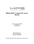
Floating-Point Mathematical Co-Processor for a Single-Chip
On-Board Computer
Tanya Vladimirova, David Eamey, Sven Keller and Prof Sir Martin Sweeting
Surrey Space Centre
School of Electronics and Physical Sciences
University of Surrey, Guildford, UK, GU2 7XH
tel: +44(0)1483 689278, email: [email protected]
Abstract: This paper is concerned with the design of a 32-bit floating-point mathematical co-processor core
using the CORDIC algorithm. The core implements the main arithmetic operations of addition, subtraction,
multiplication and division, as well as 13 elementary functions. The co-processor conforms to the IEEE-754
standard for single-precision floating-point numbers, handling overflow, underflow and special number
representations, such as infinity and not-a-number. The co-processor core was modelled in VHDL and integrated
with the LEON SPARC V8 microprocessor core. The operation of the integrated design was tested on a XILINX
Virtex XCV800 FPGA. This paper outlines the co-processor design and discusses its integration with the LEON
microprocessor core. Results, illustrating the performance of the co-processor core, are presented.
1. Introduction
Previously, work has been reported on the design of a system-on-a-chip on-board computer (SoC-OBC) for a
small satellite [1, 2, 3], consisting of soft intellectual property (IP) cores. This paper focuses on a 32-bit floatingpoint mathematical co-processor peripheral IP core for the SoC-OBC. The co-processor is based on the Coordinate Rotation Digital Computer (CORDIC) algorithm and is capable of computing 17 mathematical
functions: addition, subtraction, multiplication and division as well as square root, sine, cosine, tangent, inverse
sine, inverse cosine, inverse tangent, hyperbolic sine, hyperbolic cosine, hyperbolic tangent, inverse hyperbolic
tangent, exponential, and natural logarithm. The co-processor design conforms to the IEEE-754 standard for
single-precision (32-bit) floating-point numbers, handling overflow, underflow and special number
representations, such as infinity and not-a-number.
An RTL model of the co-processor was captured in VHDL. The functionality of the RTL design was fully
verified and debugged, leading to the final version of the VHDL code, which was then synthesized and
implemented. The co-processor was integrated with the LEON SPARC V8 microprocessor core and its operation
was tested on a XILINX Virtex XCV800 FPGA.
The paper is structured as follows. Section 2 introduces the theory behind the CORDIC algorithm. Section 3
gives details about the structure and design of the co-processor. Section 4 discusses the interface of the coprocessor with the LEON microprocessor core. System-level integration and performance results are presented
in Section 5.
2. The CORDIC Algorithm
The CORDIC algorithm was originally developed by Jack E. Volder [4] as a digital solution to real-time
navigation problems. The algorithm employs only shift and add/subtract operations, which makes it very
attractive for hardware implementation. It belongs to the “digit-by-digit” iterative numerical algorithms, which
have the property of generating one true binary digit of the result at each iteration. Generalization of the
algorithm by John Walther [5] permitted a number of functions to be implemented and extended the argument
domain. The computation scheme of the CORDIC algorithm is based on the rotation of a vector in a Cartesian
coordinate system and the evaluation of the length and angle of the vector.
In the CORDIC method, the rotation of a vector [x0 , y0 ]T by an angle θ is implemented as an iterative process,
consisting of a sequence of elementary rotations during which the initial vector is rotated stepwise by predetermined step angles α i , where i = 0,1, 2,..., n − 1 and n is the number of iterations. The elementary rotations
can be positive or negative depending on the direction of rotation, denoted by δ i ∈ {−1, 1} . The angle of rotation
θ is approximated by the sum of the n elementary rotations as follows:
θ≅
n −1
∑δ α
,
i i
(1)
i =0
The direction of the next elementary rotation is determined by the sign of the difference between the angle θ
i −1
and the i -th partial sum of step angles, θ − ∑ δ jα j . In the algorithm equations, an auxiliary variable zi serves
j =0
the purpose of accumulating the step angles and determining the sign of the next step rotation.
The rotations of the CORDIC algorithm are usually carried out in two modes, called rotation and vectoring. In
rotation mode, the input vector is rotated by a given angle, the angle accumulator zi is initialised with the
rotation angle and rotation at each iteration is aimed at making the angle accumulator converge towards zero. In
the vectoring mode the vector is rotated to the x -axis through whatever angle is necessary to align the result
vector with the x -axis.
Walther [5] has summarised the algorithm using a set of unified CORDIC iteration equations as follows:
xi +1 = xi − myiδ i 2 −i
(2)
yi +1 = yi + xiδ i 2 −i
(3)
(4)
zi +1 = zi − δ iα i
where δ i = sign( zi ) and i = 0,1, 2,..., n − 1 . The mode variable, m , takes the value of 1 , 0 or −1 for circular,
linear and hyperbolic groups of functions, and the elementary angle of rotation, α i , is an arctangent, a power of
two or a hyperbolic arctangent, correspondingly.
Using the unified CORDIC iteration equations, we can compute a wide range of mathematical functions.
Figure 1, adapted from Walther [5], shows the outputs of the algorithm, xn , yn and zn , for the three groups of
functions, where the diagrams in the left-hand column represent rotation mode and the diagrams in the righthand column – vectoring mode.
x
x
K1 (x cos z – y sin z)
y
y
K1 (y cos z + x sin z)
z
z
0
CIRCULAR (m=1), δ = sgn z
x
x
K1 (x2 + y2)1/2
y
y
0
z
z
z + tan-1(y/x)
CIRCULAR (m=1), δ = - sgn y
n -1
K1 = 1 / Π (1 + 2-2i)1/2 for n iterations
i=0
x
x
x
y
y
y + xz
z
z
0
x
x
0
y
y
0
z
z
z + y/x
LINEAR (m=0), δ = sgn z
LINEAR (m=0), δ = - sgn y
x
x
K -1 (x cosh z – y sinh z)
y
y
K -1 (y cosh z + x sinh z)
z
z
0
HYPERBOLIC (m=-1), δ = sgn z
x
x
K -1 (x2 - y2)1/2
y
y
0
z
z
z + tanh-1(y/x)
HYPERBOLIC (m=-1), δ = - sgn y
n -1
K -1 = 1 / Π (1 – 2-2i)1/2 for n iterations
i=0
Figure 1. Input-output relationships for CORDIC modes.
2
The input arguments values in the input-output relationships in Figure 1 can be chosen so as to make calculation
of functions like x ⋅ z , y ÷ x , sin z , cos z , tan −1 y , sinh z , cosh z and tanh −1 y possible. From these, we are
then able to generate the following composite functions:
tan z = sin z / cos z
tanh z = sinh z / cosh z
exp z = sinh z + cosh z
ln w = 2 tanh −1 ( y / x) ,
1/ 2
w
= (x − y ) ,
2
2 1/ 2
(5)
(6)
(7)
where x = w + 1 and y = w − 1
(8)
where x = w + 1 / 4 and y = w − 1 / 4
(9)
In addition to this, Andraka [6] shows how arcsine may also be calculated. This is achieved by starting with a
unit vector on the x -axis, then rotating it so that its y component is equal to the input argument. Using this
method, δ is obtained in a different way, as it is defined as:
⎧+ 1 if yi < c
δi = ⎨
(10)
⎩− 1 if yi ≥ c
where c is the input argument.
Stepping through the iteration equations in circular mode ( m = 1 ) produces:
xn = [( K n x0 ) 2 − c 2 ]1/ 2
(11)
yn = c
(12)
zn = z0 + arcsin[c /( K n x0 )]
(13)
The arccosine can be computed from the arcsine by subtracting 90° from the result and inverting the sign of this
new result.
The CORDIC equations impose a limited domain upon the arguments for the evaluated mathematical functions.
In order to make the algorithm work over the whole range, the inputs and outputs need to be scaled. A table of
pre-scaling identities is given in Table 1, taken from Walther [5].
Table 1. Pre-scaling identities for mathematical functions.
Identity
Domain
{ sin D if Q mod 4 = 0 }
sin(Q 90 + D) = { cos D if Q mod 4 = 1 }
|D| < 90
{ -sin D if Q mod 4 = 2 }
{ -cos D if Q mod 4 = 3 }
{ cos D if Q mod 4 = 0 }
cos(Q 90 + D) = { -sin D if Q mod 4 = 1 }
|D| < 90
{ -cos D if Q mod 4 = 2 }
{ sin D if Q mod 4 = 3 }
tan(Q 90 + D) = sin(Q 90 + D) / cos(Q 90 + D)
|D| < 90
tan-1(1/y) = 90 – tan-1 (y)
|y| < 1
sinh(Q loge 2 + D) = (2Q/2)[cosh D + sinh D – 2-2Q(cosh D – sinh D)]
|D| < loge 2
cosh(Q loge 2 + D) = (2Q /2)[cosh D + sinh D + 2-2Q(cosh D – sinh D)] |D| < loge 2
tanh(Q loge 2 + D) = sinh(Q loge 2 + D) / cosh(Q loge 2 + D)
|D| < loge 2
0.17 < T < 0.75
tanh-1(1 – M2-E) = tanh-1(T) + (E/2) loge 2
where T = (2 – M – M2-E) / (2 + M – M2-E)
for 0.5 ≤ M < 1, E ≥ 1
exp(Q loge 2 + D) = 2Q(cosh D + sinh D)
|D| < loge 2
loge (M2E) = loge M + E loge 2
0.5 ≤ M < 1.0
sqrt(M2E) ={ 2E/2 sqrt(M),
if E mod 2 = 0 }
{0.5 ≤ M < 1.0
{ 2(E+1)/2 sqrt (M/2), if E mod 2 = 1 }
{0.25≤ M/2 < 0.5
(Mx2Ex)(Mz2Ez) = (MxMz)2Ex + Ez
0.5 ≤ Mz < 1.0
(My2Ey) / (Mx2Ex) = (My / 2Mx)2Ey – Ex + 1
0.25 ≤ My / 2Mx < 1.0
Before any development work was carried out in VHDL, the floating-point operation of the CORDIC algorithm
was fully investigated via software modelling at bit-level using the C programming language.
3
3. Design of the Co-processor IP Core
The input/output interface of the CORDIC maths co-processor core is shown in Figure 2. There are two 32-bit
wide input ports for the two possible arguments A and B. There is a 6-bit input port “OP”, which specifies which
function is to be calculated, according to encoding shown below in Table 2 of Section 3.2. A “GO” input signal
is to tell the co-processor that the desired values are on the inputs and to begin calculation. There is also a clock
input signal. In terms of output ports, there is the 32-bit result output and also a “Done” output signal to indicate
the end of a computation.
A
B
Result
Co-processor
OP
GO
Done
CLK
Figure 2. Input/output interface of the maths co-processor module.
3.1 Structure of the Maths Co-Processor
The VHDL model of the co-processor IP core, “Math.vhd”, has a multi-level hierarchical structure. Figure 3
shows the top level of the design hierarchy, consisting of the following blocks - a generic iterative CORDIC
module, eight pre-scaling modules (Prescale000 to Prescale111), eight post-scaling modules (Postscale000 to
Postscale111), multiplexers and a finite state machine (“SM_scale.vhd”). Due to the fact that the CORDIC
algorithm will only work for arguments within a certain domain, as discussed in Section 2 above, there are three
stages in the computation. Any input arguments outside the specified domain are first of all scaled to within it,
before being input to the iterative CORDIC module at the centre of the co-processor. The results from the
CORDIC module finally pass through post-scaling blocks, to give the true result.
Prescale000
Postscale000
CORDIC
Module
Prescale001
Postscale001
…
…
Finite
State
Machine
GO
Done
Fig. 3. Top-level block-diagram of the co-processor IP core.
The generic computational CORDIC module in Figure 3 implements the unified equations (2)-(4) of the
CORDIC algorithm in Section 2. The module is able to evaluate functions in the circular ( m = 1 ), linear ( m = 0 )
and hyperbolic ( m = −1 ) modes, as shown in Figure 1. The design work also involved providing support for
vectoring mode and for computing arcsine and arccosine.
4
The 16 scaling modules (8 pre-scaling and 8 post-scaling modules) implement the scaling identities in Table 1. A
complex state machine, “SM_scale.vhd”, comprising different branches for each operation group, controls the
scaling operations, needing to be carried out. Multiplexers could then be used to select from which pre-scaling
block to take the x , y , z , c , δ and m inputs for the CORDIC module and also which post-scaling block to
take the final result from. The diagram presented in Figure 3 only includes two sets of pre-scaling and postscaling blocks and only the x , y and z inputs are connected to the CORDIC module.
Main components of the generic CORDIC module in Figure 3 are three 32-bit floating-point adders/subtractors
and a state machine “SM_CORD.vhd” controlling its operation.
3.2 Extending the Domain
Extending the domain of the arguments involved first of all scaling the input argument to be within a certain
domain as specified in Table 1, starting the CORDIC module with this new argument and then scaling of the
result from the CORDIC module so as to obtain the desired result.
Some of the functions can be grouped together, an obvious example being sine, cosine and tangent, as CORDIC
can compute the sine and cosine of the angle at the same time. All that needs to be done is for the post-scaling to
select either one of the two outputs, or channel both the outputs back into the division pre-scaling block, so as to
produce the result for tangent. Similarly, it is logical to group together sinh, cosh and tanh. Also, as exponential
is computed by addition of the sinh and cosh results, this can also be included in the group. Taking this argument
a little further yields the grouping of the trigonometric and the hyperbolic functions together. The pre-scaling for
both involves dividing the original argument by a constant to obtain a quotient and a remainder. The only
difference is that this constant is 90º for the trigonometric functions and loge 2 otherwise. Although different
post-scaling would be needed, this could still be implemented in the same post-scaling block, but with
multiplexers to select which result is taken. Table 2 shows the result of grouping functions together. It can be
seen that each operation now has a 6-bit representation, with the 3 most significant bits being the group number
and the least significant 3 bits referring to a specific function within that group.
It can be noticed that after the first two groups, it proved difficult to group any of the remaining functions
together, due to the differences between the scaling techniques used. This is in spite of the fact that the loge
function is being computed using the tanh-1 function.
Table 2. Grouping of functions for pre-scaling and
post-scaling.
Function
Group
Number
sin
cos
tan
sinh
cosh
tanh
exp
000
000
000
000
000
000
000
000
001
010
100
101
110
111
sin-1
cos-1
001
001
000
010
tan-1
010
000
tanh-1
011
000
sqrt
100
000
multiplication
101
000
division
110
000
loge
111
000
5
3.3 IEEE Standard 754 Special Cases
As well as the way in which numbers are usually represented, the IEEE Standard 754 [7] specifies, for single
precision numbers, the special representations shown in Table 3.
Table 3. Special representations for single-precision floating-point numbers.
Sign bit
0
0
1
0 or 1
Exponent
0
255
255
255
Mantissa
0
0
0
Not 0
Number represented
Zero
+∞
-∞
Not-a-number (NaN)
If the result of a computation carried out will have magnitude greater than is possible to represent normally with
a single-precision number (1.999 x 2127), then the magnitude of this number must instead be set to infinity. This
is known as overflow. Similarly, if the result of a computation will have magnitude less than is possible to
represent (1.0 x 2-126), then the result should instead be set to zero. This is known as underflow.
Giving certain arguments to a particular operation might result in one of the special cases, listed in Table 3
above, being the desired result. For instance, we have no way here of representing imaginary numbers, so if a
negative number is given as the argument for a square root calculation, we will want to return the not-a-number
(NaN) representation. Also, if a NaN representation is given as an input to an operation, then the result should
also be NaN. There are a number of cases like that when the result can be determined directly, given the
arguments. A list of these special cases is shown in Table 4.
Table 4. Special cases.
Operation
Argument A
Argument B
Result
sin/cos/tan/sinh/cosh/tanh/
sin-1/cos-1/tan-1/tanh-1/exp
sin/cos/tan/sinh/cosh/tanh/
sin-1/cos-1/tan-1/tanh-1/exp
Sqrt
Sqrt
Sqrt
multiplication
multiplication
multiplication
multiplication
multiplication
multiplication
multiplication
multiplication
multiplication
multiplication
division
division
division
division
division
division
division
ln
ln
ln
ln
±∞
N/A
NaN
NaN
N/A
NaN
+∞
Any negative
NaN
Any number
NaN
±∞
Any number
+∞
+∞
-∞
-∞
0
Any number
Any number
NaN
±∞
Any number
±∞
0
Any number
0
Any negative
NaN
+∞
N/A
N/A
N/A
NaN
Any number
Any number ≠0
±∞
-∞
+∞
+∞
-∞
Any number
0
NaN
Any number
±∞
±∞
Any number
Any number
0
N/A
N/A
N/A
N/A
+∞
NaN
NaN
NaN
NaN
±∞
±∞
-∞
+∞
-∞
+∞
0
0
NaN
NaN
NaN
0
±∞
0
±∞
NaN
NaN
NaN
+∞
Eight control signals are used to detect any of the special cases based on the values of the inputs. Two of these
are the sign bits of each of the two inputs (0 for positive, 1 for negative). The remaining control signals are
obtained by connecting the eight exponent bits of each input to both an “allzero” detector and an “allone”
detector, and the twenty-three mantissa bits of each to an “allzero” detector. The “allzero” detector outputs logic
‘1’ when all input bits are zero, logic ‘0’ otherwise. The “allone” detector performs a similar function, detecting
ones.
It is ensured that all the eventualities are handled if the inputs are special case numbers. As long as the values of
the input arguments are normal numbers, they will be scaled, so as to be within the domain required by the
6
CORDIC module. The CORDIC module will then compute accurate results for the mathematical operation. The
state machine of the maths co-processor “SM_scale.vhd” checks for any of the aforementioned special cases. If
any of these occur, then the machine jumps straight to the “Done” state, at the same time setting a certain output
signal to logic ‘1’. There are four of these output signals, to show that the result should be either +∞, -∞, zero or
not-a-number. In the top-level co-processor module, which contains the state machine, a 3-bit number is set
dependent on these output signals from the state machine. This 3-bit number is then used as the input to a
multiplexer, to select an appropriate result. This result can be either one of the special number representations or
a result output from the computational part of the co-processor (a result that has been calculated in the normal
way).
Of the functions computed by the co-processor, the only ones capable of producing overflow or underflow are
sinh, cosh, tanh, multiplication and division. It is in the post-scaling blocks where overflow and underflow are
handled. Adding or subtracting a number to or from the exponent of the result achieves the final part of postscaling for each of the appropriate functions. This number comes from the corresponding pre-scaling block and
is dependent on how much the original input argument had to be scaled. The addition or subtraction of the
exponent is carried out with a fixed-point binary adder using the value of its most significant carry output signal
as an indication of overflow or underflow. Programming in this logic, along with some checks that the final value
of the exponent was not either 0 or 255 (all zeroes or all ones), enabled select signals to be produced in the postscaling blocks. These were then connected to multiplexers, to select either the scaled result, positive or negative
infinity, or zero as our final result.
4. Interfacing the Co-processor to the LEON Microprocessor Core
4.1 Generic Co-Processor Interface
The LEON processor provides a generic interface enabling a co-processor to be connected. The interfacing of a
user-defined co-processor to LEON is described in the LEON Processor Users Manual [8]. This interface allows
the co-processor’s execution unit to operate in parallel to the integer unit (IU). Figure 4 shows a waveform
diagram defining the timing for all of the co-processor inputs and outputs [8].
As can be seen from Figure 4 the start signal should go high on a rising clock edge. For the one clock cycle that
this is high, the correct opcode will be available on the opcode input. On the following clock rising edge, the
load signal will go high and the two operands will be available on the op1 and op2 inputs. At the same time as
the load signal going high, the busy output from the co-processor must go high, and stay high until at least one
clock cycle before the correct result; condition codes (cc) and exception (exc) will be available on the
corresponding outputs.
Figure 4. Timing diagram for generic co-processor interface.
Although 64-bit operands and results are allowed for in the VHDL model of LEON, the co-processor was
designed to handle single-precision numbers, which need only 32 bits. Thus it was decided that the co-processor
would use only the 32 least significant bits of the inputs and outputs values. It should also be noted that 10-bit
opcodes are used.
7
Being a reduced instruction set computer (RISC) architecture, it is one of the features of the SPARC standard
that all computational type of operations are carried out exclusively register-to-register [9]. To facilitate this, a
register file consisting of thirty-two 32-bit registers is included in the design of the co-processor unit as
illustrated in Figure 5. There are specific co-processor load and store operations, which are used to move data
between co-processor registers and memory locations.
The basic principle of performing a co-processor operation follows these steps:
1. Loading the operands to the coprocessor register.
2. Asserting the start signal together with a valid opcode to start execution.
3. After finishing the operation the co-processor writes the results back to a coprocessor register.
4. A store operation writes the results back to memory.
Figure 5. Interface between the LEON processor and the co-processor.
4.2 Co-processor Operation Codes
The way in which the co-processor commands are defined is detailed in the SPARC Architecture Manual [9].
Two co-processor operate commands are provided, cpop1 and cpop2, each of which carry a 9-bit opcode
segment. The formats for these two instructions are shown in Table 5. In this table, “rd” represents destination
register, “rs1” - source register 1 and “rs2” - source register 2. The 10-bit opcode passed to the co-processor is
made up of a 0 or a 1, for cpop1 and cpop2 respectively, followed by the 9-bit opcode supplied with these
commands in field opc, bits 5 to 13.
Table 5. Format of the co-processor operate instructions.
Command
cpop1
cpop2
31-30
10
10
29-25
rd
rd
24-19
110110
110111
18-14
rs1
rs1
13-5
opc
opc
4-0
rs2
rs2
The co-processor design, described in Section 3 above, already makes use of 6-bit opcodes, so it was decided to
simply add on an extra four ‘0’ bits at the most significant end of the opcode number to make these up to 10-bit
opcodes. Only the cpop1 command is actually used.
In order to implement the co-processor interface specification [8] in VHDL, a “co-processor wrapper” was
created. This would contain the co-processor within itself, and implement suitable logic to map from the LEON
interface to the co-processor module.
Several modifications had to be made to the LEON VHDL code so that it would interface with the co-processor
correctly. Next, LEON had to be configured to accept the co-processor. Different configurations for LEON are
stored as constant records in the “target.vhd” file. The first stage was to create a new integer unit configuration,
as it is this part that decides whether or not the user-defined co-processor is enabled. A new LEON configuration
record also had to be created to make use of this new IU. Once again, this was based on an existing
configuration, with only the IU being altered:
8
constant fpga_2k2k_softprom_cp : config_type := (
synthesis => syn_gen, iu => iu_fpga_v8_cp, fpu => fpu_none,
cp => cp_cpc,
cache => cache_2k2k, ahb => ahb_fpga, apb => apb_std,
mctrl => mctrl_mem16,
boot => boot_mem, debug => debug_disas, pci => pci_none,
peri => peri_fpga);
Finally, the “device.vhd” file had to be altered to select this new configuration record.
5. System-Level Integration and Performance Results
The co-processor was integrated with the LEON SPARC V8 (LEON-2, version 1.0.9) microprocessor core and
its operation was tested on a XILINX Virtex XCV800 FPGA using the XSV800 [10] prototyping board as
shown in Figure 7. The bitstream was downloaded to the FPGA either directly from host PC 2 or indirectly from
the on-board flash memory. Communication with LEON was carried out from host PC1 via a serial connection.
Figure 7. Integration of the LEON processor and the co-processor core.
The Real Time Executive for Multiprocessor Systems (RTEMS) [11] is an open source real-time operating
system (RTOS), which provides a high performance environment for embedded systems. It supports preemptive
multitasking capabilities, multiprocessor support task prioritization and intertask communication and
synchronization. The RTOS RTEMS was installed on the LEON processor and software applications were run
with and without its support as illustrated in Figure 8.
Figure 8. Running software applications on LEON with and without RTEMS.
Major problem in implementing (SPARC) co-processor support for a conventional C-program is, that the
compiler cannot invoke the operations of the co-processor directly. In order to achieve that, a number of
assembly language routines have to be “hard-coded” within the user C-program for each function, which
requires deep knowledge of the underlying hardware by the application programmer. This may be feasible for
small programs but it is truly not applicable to larger “real-world” applications. Nested co-processor calls are
almost impossible using such a coding-style.
9
Therefore an additional mathematical software library “cpmath” has been developed in the programming
language C. The developed C-library provides an application program interface (API) and therefore removes the
need to use assembly language code to support co-processor function calls in a user program. The library is built
into a single library file (libcpmath.a) using a Makefile. If a program now wants to make use of the co-processor
operations, the library has to be linked to the program. Either copying the library to the standard library search
path or adding the path where the library resides to the search path using gcc options <PATH_TO_LIBRARY>
and -lcpmath in addition to the standard options can do this.
The Whetstone floating-point benchmark program was used to test the performance of the floating-point coprocessor. As the LEON core does not include a floating-point processor, the usual way to deal with floatingpoint calculations is to use the -msoft-float option during compile time, which emulates floating-point unit
(FPU) calls.
In order to use the mathematical co-processor with the newly built math-library it was necessary to make the
Whetstone test program compatible with the format of the co-processor library functions. For this purpose
changes were introduced in two of the most important modules of the test. As an example, changes in module 7
of the Whetstone program are shown in Figure 9, where the co-processor functions are used in the
#ifdef CP_ENABLE clause whereas in the #else clause the original code is used. It can be seen that, with the
use of the cpmath library the co-processor function calls are much easier to implement compared to the
alternative method of assembly language coding for each function call. However, it can also be seen, that
replacing even two lines of original code by co-processor calls can sometimes be rather complicated.
#ifdef CP_ENABLE
a = cpmul(t,
cpatan(cpmul( t2,
cpmul(cpsin(x),
cpdiv(cpcos(x),
(cpadd(cpcos(cpadd(x,y)),
(cpsub(cpcos(cpsub(x,y)),
1.0)))))))));
b = cpmul(t,
cpatan(cpmul( t2,
cpmul(cpsin(y),
cpdiv(cpcos(y),
(cpadd(cpcos(cpadd(x,y)),
(cpsub(cpcos(cpsub(x,y)),
1.0)))))))));
#else
c = t * atan(t2*sin(x)*cos(x) / (cos(x+y)+cos(x-y)-1.0));
d = t * atan(t2*sin(y)*cos(y) / (cos(x+y)+cos(x-y)-1.0));
#endif
Figure 9. Enabling co-processor support in a user program.
The Whetstone test was executed on four different versions of the hardware, configured as follows:
1) LEON, cp-disabled - the LEON processor on its own;
2) LEON, cp-enabled - the LEON processor with integrated co-processor core;
3) LEON/RTEMS, cp-disabled - the LEON processor on its own but running under RTEMS; and
4) LEON/RTEMS, cp-enabled - the LEON processor with integrated co-processor core and running
under RTEMS.
The co-processor has shown impressive capabilities in this test. The advantages of the co-processor can be
clearly seen from Table 6 and Figure 10, which show the performance results in seconds of execution time and
kilo Whetstone-instructions per second (KWIPS).
Table 6. Whetstone test - performance results.
10
Figure 10. Whetstone test – comparison of performance in KWIPS.
It must be noted that the maths library “cpmath”, discussed above, is totally hardware-dependent and only works
with this specific co-processor. However the principles are the same for any SPARC V8 architecture and
different co-processor op-codes can easily be adopted by changing the cpop.c, cpop.h and cpmath.h files.
6. Conclusions
This paper has described the main features of a 32-bit mathematical co-processor VHDL core for a system-on-achip on-board computer, based on the LEON SPARC V8 IP core. The co-processor is aimed at speeding up
computationally intensive applications on-board a small satellite, traditionally implemented in software, e.g.
attitude/orbit determination and control system (AODCS) algorithms.
The co-processor is compliant with the 32-bit floating-point IEEE 754 standard and implements 10 trigonometric
and hyperbolic functions, as well as square root, logarithm and exponential functions alongside the four main
arithmetic operations of addition, subtraction, multiplication and division.
Comprehensive investigation of the accuracy and correctness of the numerical results, generated by the coprocessor, was undertaken, which has shown that, overall, the accuracy of the co-processor is extremely good.
The co-processor operates at 25 MHz - when working standalone and at 2.5MHz, when integrated with the
LEON IP core. The co-processor accelerates the execution of floating-point calculations on the LEON processor.
The Whetstone benchmark runs 70% faster on the LEON processor with integrated co-processor core under
RTEMS, compared with the time it takes on LEON under RTEMS but without the co-processor. The coprocessor occupies half the size of a XILINX Virtex XCV800 chip.
The developed co-processor design is modular and its functionality can easily be tailored to a particular
application via reduction or expansion of the range of supported mathematical functions.
Acknowledgements
We would like to gratefully acknowledge financial support from the Surrey Satellite Technology Ltd. (SSTL),
which has enabled us to integrate the co-processor core with LEON under RTEMS and to run performance tests.
Thanks are due to Alex da Silva Curiel from SSTL for his encouragement and support.
References
1. H.Tiggeler, T.Vladimirova, J.Gaisler. “Designing a System-on-a-chip for Small Satellite Data Processing and
Control”, IIE Magazine on Engineering Technology, vol. 4, N 6, June 2001, pp. 38-42 .
2. D.Zheng, T.Vladimirova, M.Sweeting. “A CCSDS-Based Communication System for a Single Chip OnBoard Computer”, Proceedings of the 5th Military and Aerospace Applications of Programmable Devices and
Technologies International Conference (MAPLD'2002), D5, September 2002, Laurel, Maryland, US.
11
3. D.Zheng, T.Vladimirova, H.Tiggeler. M. Sweeting. “Reconfigurable Single-Chip On-Board Computer for a
Small Satellite” – Proceedings of the 52nd International Astronautical Federation Congress, IAF-01-U3.09,
October 2001, Toulouse, France.
4. J. Volder. “The CORDIC Trigonometric Computing Technique”, IRE Trans. Electronic Computing,
Vol EC-8, pp. 330-334, September, 1959.
5. J.S. Walther. “A Unified Algorithm for Elementary Functions”, Proceedings of the Spring Joint Computer
Conference, 1971, pp. 379-385.
6. R. Andraka. “A Survey of CORDIC Algorithms for FPGA Based Computers”, FPGA 98, Monterey CA USA,
Andraka Consulting Group, Inc, 1998.
7. “IEEE Standard for Binary Floating-Point Arithmetic”, ANSI/IEEE Std. 754-1985, The Institute of Electrical
and Electronic Engineers, Inc., 345 East 47th Street, New York, New York 10017, July 1985
8. J. Gaisler. “The LEON Processor User’s Manual”, Gaisler Research, http://www.gaisler.com/
9.“The SPARC Architecture Manual, Version 8”, SPARC International Inc.,
http://www.sparc.org/standards/V8.pdf
10. “XCV800 Prototyping Board V1.1 Manual, How to install and use your new XSV Board”, X Engineering
Software Systems (XESS) Corporation, http://www.xess.com/manuals/xsv-manual-v1_1.pdf
11. RTEMS Features, http://www.rtems.com/features.html
12