1
BIOS 203
http://bios203.stanford.edu
Winter 2013
Tutorial 1: Simulating a Solvated Protein that Contains NonStandard Residues
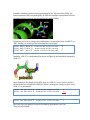
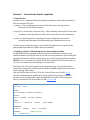
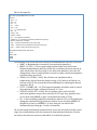
In this tutorial we will be aiming at a protein simulation of Proteorhodopsin (PR) in explicit solvent. In order to do this, we have two things to do. A. Parameter generation: Proteorhodopsin contains a protonated retinal Schiff base residue( LYR),which is a non-‐standard residue and we need to provide our own parameters.. Then we can use tleap to add explicit water solvents and finally generate the files needed for Sander to do molecular dynamics in a standard way. B. An introduction to minimization, molecular dynamics, and corresponding structure analysis for PR. This tutorial consists of following sections: 1.Do some editing of the PDB file. 2. Use tleap to Generate the Sander input files 3.Minimization and RMSD analysis of the backbone 4. MM molecular dynamics and corresponding analysis 5. Optional QM/MM dynamics and comparison (TBA). Section 1 – Do some editing of the PDB file The pdb file we will use is PDB ID: 2L6X Do this by opening PyMOL and running the command: fetch 2L6X After loading the pdb in PyMOL, you may find that it contains 20 models of the protein. For simplicity, we’re going to use only MODEL1. Make sure that you’re at the first of the 20 states, as shown above in the red rectangular. Then “File -‐> save molecule ..”, save the current molecule as a new pdb file “2l6x_001.pdb”. Now open “2l6x_001.pdb” with your favorite text editor (eg. vi) and take a look. You need to delete all of the connectivity data at the end of the PDB as this will not be used tleap. They look like this: CONECT 3277 3289 CONECT 3289 3277 3290 3318 CONECT 3290 3289 3291 3293 3319 CONECT 3291 3290 Then save the modified file as “2l6x_001_mod1.pdb” The next state is to modify some residue names that don’t match the Amber naming convention: <HIS75> and <ASP97> In amber, histidine residues can be protonated in the 'delta' position (HID), the epsilon position (HIE) or at both (HIP). In GPR, the histidine is protonated on both positions (shown as below, you should check it with PyMOL), Therefore, you need to change the residue name column of the lines of <HIS 75> to “HIP”. Finally you should got the following lines in the pdb: ATOM 863 N HIP A 75 10.964 -‐19.462 15.743 1.00 0.00 N ATOM 864 CA HIP A 75 11.800 -‐18.896 16.795 1.00 0.00 C ATOM 865 C HIP A 75 12.091 -‐17.422 16.525 1.00 0.00 C Similarly, <ASP 97> is protonated (as shown in Figure2) and should be changed to <ASH 97>. Apart from that, the charge on the OD2 atom in <ASH 97> is not correct, which is shown in the last column of the PDB file. There’s no negative charge on the O since <ASH 97> is protonated. ATOM 1240 OD1 ASH A 97 17.051 -‐17.974 14.632 1.00 0.00 O ATOM 1241 OD2 ASH A 97 16.438 -‐19.913 15.556 1.00 0.00 O1-‐ The modified result should be: ATOM 1241 OD2 ASH A 97 16.438 -‐19.913 15.556 1.00 0.00 O Now you’ve got the pdb file ready for parameter generation. Save it as “2l6x_001_mod2.pdb” Section 2 – Generate the Sander input files 1) Introduction In order to run a classical molecular dynamics simulation with Sander a number of files are required. They are: • prmtop -‐ a file containing a description of the molecular topology and the necessary force field parameters. • inpcrd (or a restrt from a previous run) -‐ a file containing a description of the atom coordinates and optionally velocities and current periodic box dimensions. • mdin -‐ the sander input file consisting of a series of namelists and control variables that determine the options and type of simulation to be run. In this section, we shall use tleap, a tool included in AmberTools to generate the prmtop and inpcrd files for explicit water solvated PR. 2)Topology and force field parameter for non-‐standard residue As mentioned at the beginning of the tutorial, Proteorhodopsin contains a non-‐
standard residue LYR and we need to provide our own parameters (frcmod file) and topology information (lib file) so that tleap can correctly generate prmtop & mdcrd. NOTE: In your own research, frcmod and lib files need to be built from scratch, but we’ll save you some time today and give you those files. The library file (.lib ) tells tleap the corresponding moiety’s charge distribution, bond order, connectivity within itself and with its neighboring moeities, and some other topology information. You can find the library file for LYR in the Tutorial1 directory (Part2):lyr.lib The force field parameter modification file (frcmod) specify the non-‐standard residue’s mass, missing bonds, angle and dihedrals as well as VDW parameters. Here is a snapshot of the frcmod file for LYR (res.frcmod) MASS n3 14.010 0.530 …. BOND n3-‐c3 320.60002 1.43560e+00 ; PARM 1 2 … ANGLE n3-‐c3-‐c 66.59001 107.10331 ; PARM 1 2 … DIHE n3-‐c3-‐c -‐o 1 6.62074e-‐01 180.000 2.000 ; PARM 2 … IMPROPER c3-‐h4-‐c -‐o 10.50000 180.0 2.0 ; PARM 1 … NONBON #VDW parameters n 1.8240 0.1700 3) Building the prmtop and inpcrd files We can now load the files into tleap and it will solvate the model and create prmtop, inpcrd for us. To start up tleap, run the following command: $AMBERHOME/bin/tleap -‐s -‐f leaprc.ff03.r1 Here the option “-‐s –f leaprc.ff03.r1” means that we are sourcing the file leaprc.ff03.r1, which is the force field file (Duan et al. 2003 ) we are going to use.
Then you can type in commands one by one in the tleap environment, just like typing bash commands in shell. Enter the following commands (only typing the portion before the commented # text in orange): source leaprc.ff03.r1 # source the force field for standard residue source leaprc.gaff #source the force field for non-‐standard residue loadamberparams res.frcmod #source the frcmod for LYR loadoff lyr.lib # load the library file for LYR MD1=loadpdb 2l6x_001_mod2.pdb #load the PR pdb file and name the molecule and MD1 check MD1 #Check the loaded molecule If tleap is running, quit it first, with the command “quit”. Run tleap, sourcing the command file: $AMBERHOME/bin/tleap -‐s -‐f leap.cmd You’ll find lines of output, including: Checking 'MD1'.... WARNING: The unperturbed charge of the unit: -‐2.000000 is not zero. Checking parameters for unit 'MD1'. Checking for bond parameters. Checking for angle parameters. check: Warnings: 1 Unit is OK. It shows that tleap has got the parameters necessary for building prmtop and inpcrd. However, the system has non-‐zero net charge. Charge neutralize our system: addions MD1 Na+ 0 #add counter ions Na+ to MD1 so that the final charge is 0 Next step, solvate the protein with explicit waters: solvateCap MD1 TIP3PBOX {16.474 -‐16.091 4.603} 40.0 What does “solvateCap” do? It adds a cap (sphere) of solvent molecules to the solute, usage: solvateCap <solute> <solvent> <position> <radius> <optional: closeness> Note, we’ve given you the center of the molecule but you could easily calculate this using a center of mass utility in PyMOL or VMD. Extra Credit (10 pts): Find a center of mass utility and use it to obtain the center of mass of each model in the full 20 model 2L6X PDB file. Prepare a table of each of these with X, Y, and Z listed separately. Tell us which utility you used. Finally save the solvated structure to prmtop and inpcrd files: saveamberparm MD1 gpr.prmtop gpr.inpcrd You can also save the solvated neutral PR model into an AMBER-‐conventional PDB file: savepdb MD1 gpr.pdb This way, you can reopen “gpr.pdb” with pymol or VMD and visually inspect your protein output to make sure that nothing has gone wrong in the preparation. Now we’ve got the sander coordinate and parameter files and we’re ready for the MM dynamics run! Section 3 – Minimization and equilibration This section will introduce sander and show how it can be used for minimization and molecular dynamics of our previously created PR model. This section of the tutorial will consist of 3 stages: 1. Minimization 2. Analysis of the minimization results. 3. Equilibration 4. Analysis of the equilibration results. 3.0) Introduction to minimization and Sander In the previous section we used the NMR structure to build a starting structure. It is always a good idea to minimize the experimental structure before commencing molecular dynamics. We used tleap to add 2 sodium ions at positions of high negative electric potential around GPR in order to neutralize it. Then we added a solvent cap of pre-‐equilibrated TIP3P water. This water has not felt the influence of the solute or charges and moreover there may be gaps between the solvent and solute. If we are not careful such holes can lead to “vacuum” bubbles forming and subsequently and instability in our molecular dynamics simulation. Thus we need to run careful minimization before slowly heating our system to 293K. We also want to allow the water to equilibrate around the solute and come to an equilibrium density. It is essential that we monitor this equilibrium phase in order to be certain our solvated system has reached equilibrium before we start obtaining results (production data) from our MD simulation. Now we are going to use sander to conduct minimization run. The basic usage for sander is as follows: sander [-O] -i mdin -o mdout -p prmtop -c inpcrd -r
restrt [-ref refc] [-x mdcrd] [-v mdvel] [-e mden] [inf mdinfo] •
•
•
•
•
•
•
•
•
•
•
•
Arguments in []'s are optional If an argument is not specified, the default name will be used. -‐O overwrite all output files (the default behavior is to quit if any output files already exist) -‐i the name of the input file (which describes the simulation options), mdin by default. -‐o the name of the output file, mdout by default. -‐p the parameter/topology file, prmtop by default. -‐c the set of initial coordinates for this run, inpcrd by default. -‐r the final set of coordinates from this MD or minimization run, restrt by default. -‐ref reference coordinates for positional restraints, if this option is specified in the input file, refc by default. -‐x the molecular dynamics trajectory file (if running MD), mdcrd by default. -‐v the molecular dynamics velocities file (if running MD), mdvel by default. -‐e a summary file of the energies (if running MD), mden by default. •
-‐inf a summary file written every time energy information is printed in the output file for the current step of the minimization of MD, useful for checking on the progress of a simulation, mdinfo by default. 3.1)Two-‐step minimization Our minimization procedure for solvated PR will consist of a two stage approach. In the first stage we will keep the PR fixed and just minimize the positions of the water and ions. Then in the second stage we will minimize the entire system. 3.1.1)Minimization Stage1 –Holding the solute fixed Here is the input file we shall use for our initial minimization of solvent and ions: min1.in gpr minimization step1, hold the protein fixed &cntrl imin = 1, maxcyc = 1000, ncyc = 500, cut = 14.0, ntb = 0, ntpr = 100, !print details to log every step ntwx = 100, !write coordinates to mdcrd every step ntwr = 100, !write restart file every step fcap = 0.1, ntr=1, / Hold the protein fixed 500.0 RES 1 235 END END NOTE: First line is for comments. Also, words after “!” are comments, which will not be explained by sander. The meaning of each of the terms are as follows: • IMIN = 1: Minimization is turned on (no MD) • MAXCYC = 1000: Conduct a total of 1,000 steps of minimization. • NCYC = 500: Initially do 500 steps of steepest descent minimization followed by 500 steps (MAXCYC -‐ NCYC) steps of conjugate gradient minimization. • NTB = 0: No periodical boundary condition used. Since sander assumes that the system is periodic by default we need to explicitly turn this off (NTB = 0) • CUT = 14.0: Use a non-‐bond cutoff of 14 angstroms. A larger cut off introduces less error in the non-‐bonded force evaluation but increases the computational complexity and thus calculation time. You will be testing this cutoff later in the problem set. • fcap=0.1. The force constant for the cap restraint potential is 1 kcal mol-‐1 angstrom-‐2. We have a solvent cap (TIP3P waters) and vacuum outside. Certainly we don’t want to see that because the system will no longer be the one we want to simulate. So, we need to add a weak restraint force on the cap. •
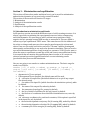
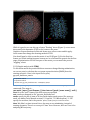
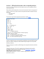
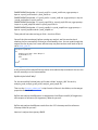
Later, we will want to test the appropriate values for this restraint in more detail. NTR = 1: Use position restraints based on the GROUP input given in the input file. GROUP input is described in detail in the appendix of the user's manual. In this example, we use a force constant of 500 kcal mol-‐1 angstrom-‐2 and restrain residues 1 through 235 (the protein). This means that the water and counterions are free to move. The GROUP input is the last 5 lines of the input file: Hold the protein fixed 500.0 RES 1 235 END END the GROUP option in the input you should Note that whenever you run using carefully check the top of the output file to make sure you've selected as many atoms as you thought you did. (Note also that 500 kcal/mol-‐A**2 is a very large force constant, much larger than is needed. You can use this for minimization, but for dynamics, stick to much smaller values around 10.) This is what your output should look like: -‐-‐-‐-‐-‐ READING GROUP 1; TITLE: Hold the protein fixed GROUP 1 HAS HARMONIC CONSTRAINTS 500.00000 GRP 1 RES 1 TO 235 Number of atoms in this group = 3672 -‐-‐-‐-‐-‐ END OF GROUP READ -‐-‐-‐-‐-‐ We are now ready to run the minimization. Note that we have an extra option on the command line (-‐ref). This specifies the structure to which we want to restrain the atoms, in this case our initial structure in the inpcrd file. We will be using the solvated prmtop and inpcrd files we created at the beginning of this tutorial. Here we’ll be using the scripts to submit our jobs to the cluster. The first few lines are commands for setting the calculation resources. The “real” sander commands start from where I commented “Here starts the sander command”. File “submin1”: #MSUB -‐S /bin/bash #MSUB -‐l nodes=1:ppn=1:gpus=7 #MSUB -‐N gpr_min1 #MSUB-‐l walltime=96:00:00 source ~/.bashrc cd ~/Tutorial1/Part3/ #Here starts your sander commands Because of the large size o-‐O f t-‐i he system, his minimization takes 1-‐0 $AMBERHOME/bin/sander min1.in -‐o mtin1.out -‐p gpr.prmtop s-‐tep c gpr.inpcrd x mins. min1.mdcrd -‐r min1.rst -‐ref gpr.inpcrd 3.1.2)Minimization Stage2 –Minimizing the entire system Now we have minimized the water and ions the next stage of our minimization is to minimize the entire system. In this case we will run 2,000 steps of minimization without the restraints this time. Here is the input file: min2.in gpr minimization step2:initial minimization whole system &cntrl imin = 1, maxcyc = 2000, ncyc = 100, cut = 14.0, ntb = 0, fcap = 0.1, ntpr = 100, !print detials to log every step ntwx = 100, !write coordinates to mdcrd every step ntwr = 100, !write restart file every step / Note, choosing the number of minimization steps to run is a bit of a black art. Running too few can lead to instabilities when you start running MD. Running too many will not do any real harm since we will just get ever closer to the nearest local minima. It will, however, waste cpu time. Here, 2,000 should be more than enough. Now run this using the following command: $AMBERHOME/bin/sander -‐O -‐i min2.in -‐o min2.out -‐p gpr.prmtop -‐c min1.rst -‐x min2.mdcrd -‐r min2.rst -‐ref gpr.inpcrd You also need to write this into a script “submin2” for submitting your job. Follow the format in submin1 and edit it. This run takes approximately 20min. 3.2) Analyzing the minimization results. 3.2.1) Visualize the minimization trajectory with VMD vmd File -‐> New Molecule (load the topology file gpr.prmtop, then load the min1.mdcrd and min2.mdcrd trajectory files into the this molecule. ) Fire up VMD and load the GPR topology file (remember to select parm7) and then load the min1.mdcrd or min2.mdcrd file into this molecule. Remember, we have not used periodic boundaries here so select "crd" (not "crdbox"). Figure 1 Figure 2 While it is good to see our big cap of water "floating" about (Figure 1) we are more interested in the dynamics of GPR so let's remove the water. Graphics-‐>Representations In Selected Atoms type: all not water and hit apply. At the same time change the drawing method to CPK. You should now be able to watch a movie of our PR (Figure 2). For the first few frames you’ll find nothing happens because we’ve restrained the protein for the first stage of minimization. For the rest part of the movie you can watch the protein “wiggling” about. 3.2.2) Simple analysis with PTRAJ To check how much the protein backbone structure changed during minimization, we can use ptraj to calculate the root mean square deviation (RMSD) from the starting structure. Here is the input file for ptraj: gpr_min_backbone_rms.in trajin min1.mdcrd trajin min2.mdcrd rms first out gpr_min_backbone.rms :1-‐235@CA,C,O,N,H Here, “trajin” is ptraj coordinate input command. Rms is one of the ptraj action commands. The usage is : rms mode [ mass ] [ out filename ] [ time interval ] mask [ name name ] [ nofit ] first: fit to the "start" frame of the first trajectory specified out: results are dumped to file “gpr_min_backbone.rms” mask: specify the list of atom to be used with Amber mask syntax. (For more on mask, see AmberTools Manual version1.5, Page146, 7.2.2 Mask syntax) ‘:1-‐235’ specify the residues, that’s the protein. ‘@CA,C,O,N,H’ specify the backbone atoms. time: We didn’t set time intervals here, because we are minimizing, instead of running dynamics. There’s no concept of “time” here. However, later we’ll use it for analyzing MD trajectory. Run ptraj : $AMBERHOME/bin/ptraj gpr.prmtop <gpr_min_backbone_rms.in plot the result with xmgrace or other graphing tool: xmgrace gpr_min_backbone.rms Or alternatively, copy the results over to your iMac and use Excel to visualize. Q: What do you notice about the RMSD of the PR backbone in relation to the restraints? What is the final RMSD? 3.3) Equilibration 3.3.1)Molecular Dynamics (heating) with restraint on the solute The next stage in our equilibration protocol is allow our system to heat up from 0 K to 293K. In order to ensure this happens without any wild fluctuations in our solute we will use a weak restraint on the solute (PR) atoms. Initially, we’ll use the Langevin temperature equilibration scheme (NTT=3) to maintain and equalize the system temperature. Since these simulations are relatively computationally expensive, it is essential that we try to reduce the computational complexity as much as possible. One way to do this is to use triangulated water, that is water in which the angle between the hydrogens is kept fixed (the TIP3P water model we used is just such kind of model). Additionally, we can constrain the O-‐H bond length in water (use SHAKE algorithm, NTC=2). This method of removing hydrogen motion can allow us to safely increase our time step to 2fs without introducing any instability into our MD simulation. Q: Why is it important to simplify our water model through fixed angle or fixed bond length in order to reduce computational cost? Why does removing hydrogen motion allow us to increase our timestep? What might our timestep limitation be if we included hydrogen motion? Short MD runs at smaller timesteps (0.5 fs) are useful for ensuring that the system can move out of unfavorable geometries without wild oscillations in the energy. Here we’re going to heat up our system with a shorter timestep (0.5fs) without SHAKE, then equilibrating with SHAKE with a step of 2fs. Here’s the input file: gpr heat up:20ps MD with res on PR &cntrl imin = 0, irest = 0, ntx = 1, cut = 14.0, fcap = 0.1, ig = -‐1, !random seed ntb = 0, tempi = 0.0, temp0 = 293.0, ntt = 3, !Langevin dynamics gamma_ln = 1.0, !Langevin dynamics collision frequency nstlim = 40000, dt = 0.0005 ntpr = 1000, !print details to log every step ntwx = 1000, !write coordinates to mdcrd every step ntwr = 1000, !write restart file every step / Keep PR fixed with weak restraints 10.0 RES 1 235 END END The meaning of the terms that didn’t show in the minimization steps are as follows: • IMIN = 0: Minimization is turned off (run molecular dynamics) • IREST = 0, NTX = 1: We are generating random initial velocities from a Boltzmann distribution and only read in the coordinates from the inpcrd. In other words this is the first stage of our molecular dynamics. Later we will change these values to indicate that we want to restart a molecular dynamics run from where we left off. • TEMPI = 0.0, TEMP0 = 300.0: We will start our simulation with a temperature, derived from the kinetic energy, of 0 K and we will allow it to heat up to 300 K. The system should be maintained, by adjusting the kinetic energy, as 300 K. • NTT = 3, GAMMA_LN = 1.0: The langevin dynamics should be used to control the temperature using a collision frequency of 1.0 ps-‐1. • NSTLIM = 40000, DT = 0.0005: We are going to run a total of 40,000 molecular dynamics steps with a time step of 0.5 fs per step, possible since we are now using SHAKE, to give a total simulation time of 20 ps. • IG=-‐1: when running production simulations with ntt=2/3 you should always change the random seed (ig) between restarts. If you are using AMBER 10 (bugfix.26 or later) or AMBER 11 or later then you can achieve this automatically by setting ig=-‐1 in the ctrl namelist. We run this using the following command. Note, we use the restrt file from the second stage of our minimization since this contains the final minimized structure. We also use this as the reference structure with which to restrain the protein: $AMBERHOME/bin/sander -‐O -‐i heatup.in -‐o heatup.out -‐p gpr.prmtop -‐c min2.rst -‐x heatup.mdcrd -‐r heatup.rst -‐ref min2.rst This takes a little less than an hour. 3.3.2)Running MD Equilibration on the whole system Now we are at 293 K we can safely remove the restraints on our protein. We will run this equilibration for 200 ps to give our system plenty of time to relax. equ.in equilibrate: &cntrl imin = 0, irest = 1, ntx = 5, cut = 14.0, ig = -‐1, !random seed fcap = 0.1, ntb = 0, ntc = 2, ntf = 2, tempi = 300.0, temp0 = 300.0, ntt = 3, !Langevin dynamics gamma_ln = 1.0, !Langevin dynamics collision frequency nstlim = 100000, dt = 0.002 ntpr = 500, !print detials to log every step ntwx = 500, !write coordinates to mdcrd every step ntwr = 500, !write restart file every step / The only things that needs to be mentioned about the inputfile is : • IREST = 1, NTX = 5: We want to restart our MD simulation where we left off after the 20 ps of simulation. IREST tells sander that we want to restart a simulation, so the time is not reset to zero but will start at 20 ps. Previously we have had NTX set at the default of 1 which meant only the coordinates were read from the restrt file. This time, however, we want to continue from where we finished so we set NTX = 5 which means the coordinates and velocities will be read from a formatted (ASCII) restrt file. • NTC = 2, NTF = 2: SHAKE should be turned on and used to constrain bonds involving hydrogen both in water and in the protein. We run this using the following command. $AMBERHOME/bin/sander -‐O -‐i equ.in -‐o equ.out -‐p gpr.prmtop -‐c heatup.rst -‐
x equ.mdcrd -‐r equ.rst This calculation takes 3.5h, be sure to leave running/queued overnight. You will also want to specify for the longer queue with the following command: msub –q longq <jobscript> Take note that you may need to use the long queue for some of the next few steps as well. Be sure to use the extended msub command where needed. 3.4) Analyzing the results to test the equilibration Before moving on to running any production MD simulations, it is essential that we check that we have successfully equilibrated our system. The properties that we’d check are as follows: Temperature RMSD 3.4.1)Analyzing the output files Let’s take a look at the output files (equ.out, heatup.out ), you can find a lot of info for each MD step that you’ve chosen to record. NSTEP = 500 TIME(PS) = 21.000 TEMP(K) = 293.53 PRESS = 0.0 Etot = -‐42085.8666 EKtot = 14258.6346 EPtot = -‐56344.5012 BOND = 665.2759 ANGLE = 1770.5041 DIHED = 2618.3474 1-‐4 NB = 903.0240 1-‐4 EEL = 12661.9741 VDWAALS = 8305.4811 EELEC = -‐83271.5664 EHBOND = 0.0000 RESTRAINT = 2.4583 EAMBER (non-‐restraint) = -‐56346.9595 To make it easier for analysis, we are going to use some scripts to extract the trajectory of each of those properties. First we can make use of the perl script from AMBER website. (process_mdout.perl). mkdir analysis cd analysis perl process_mdout.perl ../heatup.out ../equ.out This script takes a series of mdout files and will create a series, leading off with the prefix "summary." such as "summary.EPTOT", of output files. These files are just columns of the time vs. the value for each of the energy components. Q: Plot the temperature from the resulting simulations and note what you observe regarding equilibration of your system. 3.4.1)Analyzing the trajectory This is roughly the same as the ptraj analysis for minimization: equ_rms.in trajin heatup.mdcrd trajin equ.mdcrd rms first out gpr_heat_backbone.rms time 1 :1-‐235@CA,C,O,N,H Q: Plot the RMSD you get from ptraj and note what the RMSD is with constraints and then what its value is after constraints are released. Section 4 – MM molecular dynamics and corresponding analysis Now we’ve already at 293K with the well relaxed structure, we’re heading to the final step: production MD. Real production MD usually takes at least several nanoseconds. Here for the purpose of practice, we will only run 20ps to observe some phenomena when we adjust the input parameters: • Non-‐bond cutoff • Time Step The reference input file with appropriate parameters is called prod.in production md 20ps: &cntrl imin = 0, irest = 1, ntx = 5, cut = 14.0, ig = -‐1, !random seed ntc = 2, ntf = 2, fcap = 0.1, ntb = 0, tempi = 293.0, temp0 = 293.0, ntt = 3, !Langevin dynamics gamma_ln = 1.0, !Langevin dynamics collision frequency nstlim = 10000, dt = 0.002 ntpr = 10, !print detials to log every step ntwx = 10, !write coordinates to mdcrd every step ntwr = 10, !write restart file every step / This one is roughly the same as the input file for equilibration. We used SHAKE and time step of 2fs. Cutoff is 14 angstrom, which should be large enough for our non-‐periodic boundary simulation. Then we are going to try smaller cutoff and larger time step and see how the calculation collapses. Change the time step to 3.2 and 4 fs, respectively, and change the total step limit accordingly to keep the total run time 20ps. We’ll get prod_cut10.in, prod_cut8.in Submit the jobs in separate directories: $AMBERHOME/bin/sander -‐O -‐i prod.in -‐o prod.out -‐p gpr.prmtop -‐c equ.rst -‐x prod.mdcrd -‐r prod.rst $AMBERHOME/bin/sander -‐O -‐i prod_cut10.in -‐o prod_cut10.out -‐p gpr.prmtop -‐c equ.rst -‐x prod_cut10.mdcrd -‐r prod_cut10.rst $AMBERHOME/bin/sander -‐O -‐i prod_cut8.in -‐o prod_cut8.out -‐p gpr.prmtop -‐c equ.rst -‐x prod_cut8.mdcrd -‐r prod_cut8.rst $AMBERHOME/bin/sander -‐O -‐i prod_step3.2fs.in -‐o prod_step3.2fs.out -‐p gpr.prmtop -‐
c equ.rst -‐x prod_step3.2fs.mdcrd -‐r prod_step3.2fs.rst $AMBERHOME/bin/sander -‐O -‐i prod_step4fs.in -‐o prod_step4fs.out -‐p gpr.prmtop -‐c equ.rst -‐x prod_step4fs.mdcrd -‐r prod_step4fs.rst These jobs will not take too long to finish – less than 35min. Once all the jobs terminated, before running any analysis, we first need to check whether they are successfully finished or terminated by error. You can read through the output files one by one, but a more efficient way may be to write a small bash script nd call it check_jobs.sh: for file in `ls prod*.out` do numline=`grep "Run done" $file|wc -‐l` if [ $numline -‐lt 1 ] then echo $file fi done ./check_jobs.sh It will print out all the output files that seems to be abnormally terminated. You can also do this manually or at the commandline. Q: Which jobs failed? Why? For the successfully finished jobs, we’ll make a folder ‘analysis_XXX’ for each ie, analysis_prod, analysis_prod_cut10, analysis_prod_step3.2fs Then run the ‘process_mdout.perl’ script for each of them in the folders, so that we get properties for each run. Q: Plot and analyze the differences in temperature for different cutoffs (10 Angstroms) with respect to reference (14 Angstroms). What do you see? Q: Plot and analyze the different results from the 3.2 fs timestep and the reference timestep. What do you see? Now Let’s analyze the trajectory RMSD. You only need to modify the ptraj input file equ_rms.in a little bit by changing the trajin trajectory file name, output file name, and time interval. Input files: prod_rms.in, prod_cut10_rms.in, prod_step3.2fs_rms.in Output files: gpr_prod_backbone.rms, gpr_prod_cut10_backbone.rms, gpr_prod_step3.2fs_backbone.rms Q: Plot the RMSD for the different distance cutoff, timestep against the reference. What do you notice about the RMSD between all of these? We can evaluate a local backbone RMDS of the residues around the chromophore, eg. residues within 3.5 angstroms of LYR in the NMR structure. And you can imagine the only trick here is to set the correct “mask” for PTRAJ – we need to know the residue IDs. There are lots of ways for doing this. One way is to use the selection command of Pymol, and this maybe the most straightforward way. Load ‘gpr.pdb’ to PyMol, enter the command: sele br. (all within 3.5 of resn LYR) and (not resn LYR) br. Means “by residue” – extend the selection to the whole residue, namely for residue with any of its atoms inside the region, all atoms in the residue will be selected. Then just choose Menu: File -‐> Save Molecule, in the popped window, choose object “sele” to be saved as th
“sele.pdb”. You can read the residue ID from the 5 column of “sele.pdb”, but may find it tedious . A simple bash script can do this for you. grep "CA" sele.pdb |awk '{ print $5 }'|tr "\\n" "," Ah, we got the residue IDs nicely separated by commas. Now just paste this to your PTRAJ input file for backbone RMSD, run ptraj, and you’re all set. prod_rms_within3.5.in trajin prod.mdcrd rms first out gpr_prod_backbone_within5.rms time 0.02 :<residue selection from script>@CA,C,O,N,H test_cpptraj.in trajin gpr.inpcrd mask :LYR<:3.5&@CA maskout temp.txt Actually we can also select residues with the cpptraj action “mask”, if you prefer command line operation: Run cpptraj: $AMBERHOME/bin/cpptraj -‐i test_cpptraj.in -‐p gpr.prmtop And the results are dumped in “temp.txt”, with all alpha-‐C atoms whose residue is within 3.5 Angstrom of LYR. Once again we use a bash command to get the final IDs: grep CA temp.txt |awk '{ print $4 }'|tr "\\n" "," And you’ll get the same answer. For more use of cpptraj, please refer to the Amber-‐ Tools 12 Manual, Chapter 7. Q: Graph the RMSD of the near-‐LYR residues (3.5 Angstroms) and compare to that of the whole protein. Do you notice any key differences? Extra credit: Look for differences if you look at other subsets of residues. Can you identify any residues that give rise to a high RMSD to experiment? Which parts of the proteins give rise to a lower RMSD to experimental structure? Apart from RMSD, PTRAJ can keep track of lots of geometric properties, like angle , dihedral, etc. Please refer to AmberTools12 manual for details.