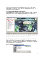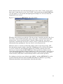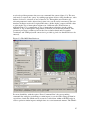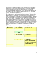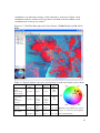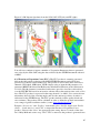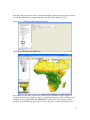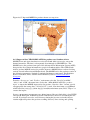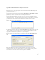
1
FACULTY OF GEO-INFORMATION SCIENCE
AND EARTH OBSERVATION
ITC
GEONETCAST
TOOLBOX
INSTALLATION, CONFIGURATION AND
USER GUIDE OF THE GEONETCAST
TOOLBOX PLUG-IN FOR ILWIS 3.7
Ben Maathuis, Chris Mannaerts
Department of Water Resources (WRS)
Martin Schouwenburg, Bas Retsios and Rob
Lemmens
Department of Geo-information Processing (GIP)
August 2010
University of Twente, Faculty ITC
i
Colofon:
University of Twente
Faculty of Geo-information science and earth observation
Department of Water Resources
Department of Geo-information Processing
Date last modified:
30 August 2010
Published version:
Version 1, contains 2 DVDs with GEONETCast sample data and CD with software
(ILWIS371 and GEONETCast Toolbox)
E-mail corresponding author:
[email protected]
Postal address:
P.O. Box 217
7500 AE Enschede
The Netherlands
Website:
www.itc.nl
Copyright:
© ITC, Faculty of Geo-Information Science and Earth Observation of the University of
Twente, Netherlands. Text and numerical material from this publication may be
reproduced in print, by photocopying or by any other means with the permission of ITC if
the source is mentioned.
Published by:
University of Twente
Faculty of Geo-Information Science and Earth Observation
Departments of Water Resources and Geo-information Processing
ii
Acknowledgement
Based on the announcement by EUMETSAT in 2004 that data from the SEVIRI
instrument (onboard of the MSG satellite) would be freely available for education and
research, at ITC an initiative started to be able to import and process the data from this
instrument. As more data became available, also through efforts of the Group on Earth
Observation (GEO), by means of global data dissemination systems – “GEONETCast”,
this process continued. The routines developed have been integrated into a toolbox, called
the “GEONETCast – Toolbox”, developed as a plug-in to be used within a generic
remote sensing and GIS freeware and open source package called “ILWIS”. Next to the
already existing “ILWIS community” hosted by “52North.org” also a new community
could be established, called “Earth Observation”, where all utilities can be freely
obtained. 52North is thanked for their support to host this website.
This development would not have been possible without the support from various
organizations. Firstly EUMETSAT’s support has been instrumental. Technical or
logistical questions, requests for trial data or establishing contacts with data providers
where handled promptly and efficiently. Also utilities developed by EUMETSAT could
be used, such as the Product Navigator. Also [email protected] was instrumental
in providing licenses for new users in Africa, specifically from Universities who wanted
to embark on “GEONETCast”.
Secondly, the ITC Directorate has been instrumental in supporting this development as
well. Next to their support to the Capacity Building component of GEO, they decided to
allocate resources for this development initiative as well, including setting up antennas,
providing data storage capacity and day to day management.
Thirdly, the collaboration within different projects with various partners from all over the
world was instrumental. Important activities to be mentioned are DevCoCast (FP-7),
AMESD and other training workshops. Through these project activities and workshops a
large group of data providers and users could be reached and their comments have helped
to further develop the toolbox. Special thanks go to VITO, JRC, INPE, INTA, RCMRD,
UCT.
It is hoped that this version of the GEONETCast toolbox will even reach a larger
audience than the 3.6 version and will be useful in integrating the ever increasing
environmental data stream for better management and planning of our resources.
iii
iv
Preface
Over the recent years many developments have taken place to provide the global user
community with large amounts of environmental data, provided free of charge and
delivered through satellite based communication systems. In order for the user
community to handle and process the data the “GEONETCast-Toolbox” has been
developed.
The GEONETCast-Toolbox allows the user to import a multitude of data types
disseminated via “EUMETCast-GEONETCast” into the freeware and open source RSGIS ILWIS package and its existing processing capability can be used for further
analysis.
This document is proving a description where to download all the freeware utilities, how
to install and configure them. The Toolbox developed is an open utility, it can be easily
modified and tuned to the user needs and furthermore it can be expanded to cope with the
increasing data stream without the need for programming skills. Next to this description
also an overview is presented on the various data types disseminated that can be imported
and processed.
Finally the document provides exercises on how to use the utilities offered and is
exploring the “GEONETCast” data stream. The exercises currently provided are
focussing on Africa and Latin America. It is foreseen that also an addition will be
provided later to cover the SE Asian – Pacific region.
The utilities provided are extensively tested using various operating systems, such as
Windows Vista, XP (various service packages) and Windows-7 and have found to be
performing in a stable manner. The toolbox currently does not work under LINUX. In
case unexpected behaviour or bugs are observed, additions to the functionality are
required or if you have developed new utilities that you want to share, please contact:
[email protected].
This document is not describing how to setup a low cost ground reception station.
Additional documentation in this respect can be found at: http://www.itc.nl/Pub/
WRS/WRS-GEONETCast or at: http://52North.org, under the “Earth Observation”
Community page. Here new additions and modifications will be posted and you can
register to a mailing list as well, to keep you updated on ongoing developments.
August 2010
Ben Maathuis and Chris Mannaerts
Department of Water Resources
ITC
v
vi
List of acronyms and abbreviations
52North
AFIS
AIDA
AMV
AVHRR
BEAM
BILKO
BRAT
BUFR
CBERS
CCD
CHC
CLAI
CMA
CSIR
CTH
DDS
DevCoCast
DMP
DN
DSLF
DSSF
DVB
ENVISAT
ESA
ET
EUMETCast
EUMETSAT
FAPAR
FDG
FDN
FDI
FENGYUN
FFDI
FTC
FTP
FVC-FCOVER
GDAL
GEO
52°North Initiative for Geospatial Open Source Software
Advanced Fire Information System
Advancing Information and Communication Technology (ICT) for
Disaster risk management in Africa
Atmospheric Motion Vector
Advanced Very High Resolution Radiometer
Basic ERS and Envisat AATSR and MERIS Toolbox
Software package for learning and teaching remote sensing image
analysis skills
Basic Radar Altimetry Toolbox
Binary Universal Form for the Representation of meteorological
data
Chinese Brazilian Earth Resources Satellite
Charge Coupled Device
CBERS CCD and HRC composite product
Cloud Analysis Image
Chinese Meteorological Agency
Council for Scientific and Industrial Research, South Africa
Cloud Top Height
Data Dissemination System
Geonetcast for and by Developing Countries
Dry Matter Productivity
Digital Number
Down welling Surface Long-wave radiation Flux
Down welling Surface Short-wave radiation Flux
Digital Video Broadcast
Environmental Satellite
European Space Agency
Evapotranspiration
A satellite based data dissemination of various (mainly satellite
based) data covering Europe and Africa
European Organisation for the Exploitation of Meteorological
Satellites
Fraction of Absorbed Photosynthetically Active Radiation
Fire Detection product from GOES
Fire Detection product from NOAA
Fire Danger Index
China's weather satellites (abbreviated FY), meaning “wind cloud”
McArthur Forest Fire Danger Index
Convective System Tracking and Evolution
File Transfer Protocol
Fraction of Vegetation Cover
Geospatial Data Abstraction Library
Group on Earth Observation
vii
GEONETCast
GEOSS
GOES
GNC
GRIB
GSOD
GUI
HRIT
HRC
HRV
ILWIS
INPE
INTA
ITC
IR
ISD
JASON
LAI
LDI
LFDI
LSA
LST
METOP
MODIS
MPE
MPEF
MSG
MTSAT
NDVI
NDWI
NIR
NOAA
PHENOKS
R
RFS
RGB
RSS
SAF
SEVIRI
SPOT
SST
SWB
TAMSAT
A global network of satellite based data dissemination systems
Global Earth Observation System of Systems
Geostationary Operational Environmental Satellites
Geonetcast
Gridded Binary data format
NOAA’s Global Summary of Day network
Graphical User Interface
High Rate Image Transmission
High Resolution Camera
High Resolution Visible
Integrated Land and Water Information System
Instituto Nacional de Pesquisas Espaciais, Brazil
Instituto Nacional de Tecnología Agropecuaria, Argentina
Faculty of Geo-Information Science and Earth Observation
Infra Red
Integrated Surface Data
The JASON altimeter program (named after the Greek
mythological hero Jason)
Leaf Area Index
Lightning Discharge Image
Lowveld Fire Danger Index
Land Surface Analysis
Land Surface Temperature
Meteorological Operational satellite programme
Moderate Resolution Imaging Spectrometer
Multi sensor Precipitation Estimate
Meteorological Product Extraction Facility
Meteosat Second Generation
Multifunctional Transport Satellites, Japanese weather satellites
Normalized Difference Vegetation Index
Normalized Difference Water Index
Near Infra Red
National Oceanic and Atmospheric Administration
Phenology Key Stages
A language and environment for statistical computing and graphics
Rainfall Satellite
Red – Green – Blue colour assignment
Rapid Scanning Service
Satellite Application Facilities
Spinning Enhanced Visible and Infrared Imager
Système Probatoire d’Observation de la Terre ou Satellite Pour
l’Observation de la Terre
Sea Surface Temperature
Small Water Bodies
Tropical Applications of Meteorology using Satellite data and
ground-based observations
viii
TIR
VGT-extract
VGT instrument
VIS
VITO
VPI
USAF
UTC
UVI
WV
XML
Thermal Infra Red
Software tool developed by VITO to import products derived from
the Vegetation instrument
Vegetation instrument onboard of SPOT
Visible
Flemish Institute for Scientific Research
Vegetation Production Indicator
United States Air Force
Universal Time Coordinated
Ultraviolet Radiation Index
Water Vapour
Extensible Markup Language
ix
Table of content
1
General installation and configuration instructions
1
1.1
1.1.1
1.1.2
1.1.3
1.1.4
1.1.5
1.1.6
1.1.7
Introduction
Download ILWIS
Download the GEONETCast-Toolbox
Download Java Runtime Environment
Download IrfanView
Download BUFRtool
Changing the ILWIS language settings, from English to French
Concluding remarks
1
1
1
2
3
3
4
4
1.2
1.2.1
1.2.2
5
5
1.2.3
1.2.4
1.2.5
Configuration of the data stream using the GEONETCast Data Manager
Introduction
General design considerations for development of the GEONETCast
Data Manager
The GEONETCast Data Manager – “Rules”
Configuring the GEONETCast Data Manager
Making the GEONETCast data available within the organisation
5
6
7
10
2
Overview of the GEONETCast Toolbox Architecture
12
2.1
2.2
2.3
2.4
2.5
2.6
2.7
2.8
2.9
2.10
Introduction
Structure of the GEONETCast toolbox
Structure of the Config.xml
General GEONETCast Toolbox Configuration – Folder settings
Configuring the data source of the MSG Data Retriever
Structure of the ILWIS GEONETCast toolbox scripts
Structure of the ILWIS GEONETCast toolbox batch routines
Changes and modifications
Advanced use
Concluding remark
12
12
15
17
17
20
21
23
23
23
3
Exploring the GEONETCast data stream using the GEONETCast
Toolbox
24
Introduction
The GEONETCast-Toolbox functionality (Config XML Version 1.0)
GEONETCast Product Navigator
GEONETCast Data Manager
MSG-HRIT, MSG Data Retriever
Calculate MSG angles
Geostationary-LRIT
Meteorological Product Extraction Facility (MPEF)
MSG – Rapid Scanning Service (RSS)
24
25
25
25
25
28
29
29
30
3.1
3.2
3.2.1
3.2.2
3.2.3
3.2.4
3.2.5
3.2.6
3.2.7
x
3.2.8 Satellite Application Facilities (SAF)
3.2.9 Real Time MSG Visualization
3.2.10 CMA products
3.2.11 TAMSAT Rainfall Product
3.2.12 SPOT VGT Products
3.2.13 DevCoCast – AIDA
3.2.14 METOP
3.2.15 JASON-2
3.2.16 Web Mapping Services
3.2.16.1
Last 24 hr MPE from EUMETSAT website
3.2.16.2
Fire Service for Africa
3.2.16.3
MPE and RFS to Google
3.2.16.4
Surface pressure forecast over Europe
3.2.16.5
Integrated Surface Data (ISD)
3.2.17 To other applications
3.2.17.1
Export to BILKO
3.2.17.2
Export to R
3.2.18 Configuration and folder settings
4
30
30
32
32
32
34
35
35
35
35
36
36
36
36
37
37
37
37
Exercises using data from GEONETCast, applying ILWIS and the
GEONETCast toolbox
38
4.1
4.1.1
4.1.2
4.1.3
4.1.4
4.1.5
4.1.6
4.1.7
4.1.8
Import and visualization of data from MSG, GOES 11-13 and METOP
Data import and visualization from Meteosat Second Generation (MSG)
Construct a daytime Microphysical (DMP) colour scheme composite
The MSG water vapour channel and the thermal channel
Multi temporal data import, processing and visualization
Import of the HRV channel
Geostationary LRIT, example of GOES 11 and GOES 13
Geostationary LRIT, example of Meteosat 7
Import of METOP AVHRR/3
38
38
42
45
49
51
52
54
55
4.2
4.2.1
Import products generated by the Meteorological Product Extraction
Facility (MPEF)
Import and processing of MPEF data
58
58
4.3
4.3.1
4.3.2
4.3.3
4.3.4
4.3.5
4.3.6
4.3.7
Import products generated by the Satellite Application Facility (SAF)
Surface Albedo
Down-welling surface short-wave and long-wave radiation fluxes
Land Surface Temperature (LST)
Evapotranspiration (ET)
Fraction of Vegetation Cover (FVC)
Leaf Area Index (LAI)
Fraction of Absorbed Photosynthetically Active Radiation (FAPAR)
63
64
64
65
65
67
68
68
xi
4.4
4.4.1
Import products generated by the SPOT Vegetation Instrument
Import of (multi-temporal SPOT VGT Africa data (NDVI, FCOVER,
LAI, PHENOKS), data quality assessment using status map
4.4.1.1
Import of a 10-day NDVI product from VGT Africa
4.4.1.2
VGT Africa NDVI correction using Status Map
4.4.1.3
Deriving statistical information, aggregated per province, using
NDVI map for Kenya
4.4.1.4
Deriving pixel based and aggregated time series information
Using a NDVI map list
4.4.2 Use of some SPOT Vegetation Data available for Latin America
4.4.2.1
Import of 10-day NDVI, NDWI and DMP products for Latin
America
4.5
Import of products generated by DevCoCast for Latin America
4.5.1 Use of DevCoCast products available for Latin America
4.5.2 Import of products from INPE
4.5.2.1
INPE rainfall product: RFS
4.5.2.2
Import of FTC, FDG, FDN, LDI, UVI and CBERS-CHC
4.5.2.3
Import of 15 day and monthly Normalized Difference Vegetation
Index – South America
4.5.3 Import of products from INTA
4.6
70
70
70
74
78
81
87
87
90
90
92
92
92
93
94
4.6.5
4.6.6
Import of Fire products disseminated through the DevCoCast and AIDA
initiatives, MPEF and MODIS Fire data, examples using Lowveld FDI,
McArthur FDI and the MPEF (MSG based), MODIS derived fire products,
the TAMSAT 10 day rainfall product and CBERS merged product
95
Import and processing of the Lowveld and McArthur Forest Fire Danger
Indices
95
Importing the MPEF FIRE product
98
Import of the CSIR MODIS-AFIS fire product over Southern Africa
99
Import of the MODIS Aqua and Terra Fire Product (import multiple
MODIS Fire product over a region, both Terra and Aqua from NOAA)
100
TAMSAT 10 day rainfall product over Africa
101
Colour Composite CCD-HRC CBERS – Africa
102
4.7
4.7.1
4.7.2
4.7.3
4.7.4
4.7.5
External Web Mapping Services
Last 24 hr MPE from EUMETSAT Website
Fire Service for Africa
MPE and RFS to Google
Surface Pressure Forecast over Europe
Integrated Surface Data (ISD)
4.6.1
4.6.2
4.6.3
4.6.4
4.8 To other applications
4.8.1 Export to BILKO
4.8.2 Export to R
103
103
103
103
105
105
107
107
107
xii
4.9
Diurnal variability of LST and ET – Multi temporal data import using
batch looping routines, South America
Appendix 1:
Appendix 2:
Appendix 3:
108
Other freeware utilities that can be used in conjunction with
ILWIS3.7
113
Structure of the sample data provided on DVD(s) and
“Earth Observation” Community Website
115
MSG Data Retriever settings for exercise 4.1
117
xiii
List of Tables
Table 3.1:
Table 3.2:
SEVIRI channels and their applications
SPOT VGTAfrica product details
26
32
Table 4.1:
Typical daytime convective development of clouds and related
colour scheme
AVHRR/3 spectral channel details and their primary use
43
55
Table 4.2:
xiv
List of Figures
Figure 1.1:
Figure 1.6:
The Geonetcast-toolbox main and sub menu structure under
ILWIS37
Changing the ILWIS menu language
Location of the Geonetcast Data Manager in the Toolbox menu
Selection of the input configuration file
The Geonetcast Data Manager, showing the menu as defined by
the text file GNC_DataManager.txt
Default Data Manager configuration file
8
9
Figure 2.1:
Figure 2.2:
Figure 2.3:
Figure 2.4:
Figure 2.5:
Figure 2.6:
Figure 2.7:
The GEONETCast toolbox plug-in Graphical User Interface
Toolbox sub-directory structure
Popup menu for import, example MET7
Setting of the in and output directory structure for SAF Africa
Meteosat Second Generation Data Retriever
Data Sources Menu
Create a new HRIT MSG2 data source folder
12
13
16
17
18
18
19
Figure 3.1:
Figure 3.2:
Figure 3.3:
Overall concept of the GEONETCast-Toolbox
The MSG Data Retriever
Example of Sun (for 21 June 2006, 12.00 UTC) and MSG satellite
zenith angles
Example of a global thermal composite
Layout of the various components for Real Time MSG
visualization
24
27
The main ILWIS menu and the active catalogue
Selection and import of MSG channels using the Data Retriever
Band assignment for visualization
Daytime standard colour scheme MSG: IR_016, VIS008, VIS006
in RGB
Displaying vector data
Import settings to construct Daytime Microphysical Colour
Scheme composite
DayTime Microphysical Colour Scheme, VIS006, IR_039 and
IR_108 in RGB
Absorption of water and ice by clouds for the various MSG
Channels
Different reflectivity of snow clouds at 0.6, 0.8 and 1.6 microns
Import of the MSG water vapour and thermal infrared channels
Imported WV channel (left) and TIR channel (right) for the same
timestamp
Irradiance and absorption for the various MSG channels
Contributions to Water Vapour and IR channels
38
39
40
Figure 1.2:
Figure 1.3:
Figure 1.4:
Figure 1.5:
Figure 3.4:
Figure 3.5:
Figure 4.1.1:
Figure 4.1.2:
Figure 4.1.3:
Figure 4.1.4:
Figure 4.1.5:
Figure 4.1.6:
Figure 4.1.7:
Figure 4.1.8:
Figure 4.1.9:
Figure 4.1.10:
Figure 4.1.11:
Figure 4.1.12:
Figure 4.1.13:
2
4
7
7
28
29
31
40
41
42
43
44
44
45
46
46
47
xv
Figure 4.1.14:
Figure 4.1.15:
Figure 4.1.16:
Figure 4.1.17:
Figure 4.1.18:
Figure 4.1.19:
Figure 4.1.20:
Figure 4.1.21:
Figure 4.1.22:
Figure 4.1.23:
Figure 4.1.24:
Map Calculation window
Import time series of MSG images, transformed into temperature
MapList Calculation window
MSG Data Retriever settings for HRV import
Imported HRV image
GOES 13 (GOES-East) disk of 19 May 2010, at 18:00 UTC,
channel 007
GOES 11 (GOES-West) disk of 19 May 2010, at 20:00 UTC,
channel 007
Meteosat 7 disk of 18 January 2010, at 0900 UTC, channel 007
Create MapList of the visible and NIR channels, transformed to
byte images
AVHRR/3 image (morning overpass) of 10 May 2010
Coverage of the various 3 minutes AVHRR/3 images
Figure 4.2.1: Input and output directory specification using the Toolbox Folder
Configuration
Figure 4.2.2: Classified cloud mask map of 20 January 2010, 12:00 UTC
Figure 4.2.3: Multi Sensor Precipitation Estimate of 20 January 2010,
12:00 UTC
Figure 4.2.4: MPE over a daytime microphysical colour scheme composite
Figure 4.2.5A:
Imported products from MPEF: CLAI and CTH
Figure 4.2.5B:
Imported products from MPEF: AMV and FIRA
Figure 4.3.1: Input and output directory specification using the Toolbox Folder
Configuration
Figure 4.3.2A:
Imported products from the LSA SAF: Albedo and DSSF
Figure 4.3.2B:
Imported products from the LSA SAF: LST and ET
Figure 4.3.3: LSA SAF vegetation products Fraction of Vegetation Cover
(FVC), Leaf Area Index (LAI) and (Fraction of Absorbed
Photosynthetically Active Radiation FAPAR)
Figure 4.4.1: VGT4Africa NDVI import window
Figure 4.4.2: The imported NDVI map
Figure 4.4.3: Imported NDVI, LAI, FCOVER and PHENOKS (phstart, phhalf
and phlength) VGT4Africa products of 20091201
Figure 4.4.4: The NDVI Status Map flag filter matrix
Figure 4.4.5: The DIV and MOD operators from the ILWIS command line
Figure 4.4.6: Map Calculation expression to extract the relevant NDVI flags
and resulting output map
Figure 4.4.7: Map calculation to correct the NDVI map using the flagged status
map and resulting corrected NDVI map
Figure 4.4.8: Create Sub Map of Kenya, sub map details and output map created
Figure 4.4.9: Create new output column table with aggregated statistics, grouped
per province, using the function average for the NDVI
Figure 4.4.10: NDVI sub map of Kenya and aggregated statistics appended to
47
49
50
51
51
52
53
54
56
57
57
58
59
60
61
62
63
63
66
67
69
71
71
73
74
75
76
77
78
79
xvi
map table
Figure 4.4.11: NDVI sub map of decade 1, 2009 and the map list graph for
the whole time series for a selected pixel location
Figure 4.4.12: Average NDVI for 2009 and pixel information window with
other statistics
Figure 4.4.13: Classified NDVI difference map and VPI class map of 20091201
Figure 4.4.14: The NDVI (left) and fCover (right) maps over Kenya,
for 20091201
Figure 4.4.15: VGT4Africa NDVI import window
Figure 4.4.16: The imported NDVI map
Figure 4.4.17: Imported NDWI and DMP for 20100401
80
82
83
85
86
88
88
89
Figure 4.5.1: DevCoCast Website
Figure 4.5.2: Latin American data providers and products
Figure 4.5.3: GNC Toolbox import routines for the Latin American
DevCoCast service
90
91
Figure 4.6.1: LFDI, fire danger values and associated fire danger classification
Figure 4.6.2: McArthur Forest Fire Danger Index (FFDI)
Figure 4.6.3: Selection of statistical function “correlation” applied to LFDI and
FFDI
Figure 4.6.4: FFDI versus LFDI scatter plot and polynomial function
Figure 4.6.5: Imported MPEF fire product shown as a map view
Figure 4.6.6: MODIS fire point maps over southern Africa, of 2010,
julian day 027
96
97
91
97
98
99
101
Figure 4.7.1: 24 hr aggregated MSG based MPE downloaded from the ITC-FTP
site, displayed on Google Earth for 01 May 2010
104
Figure 4.7.2: GSOD station locations and the pixel information window
106
Figure 4.7.3: Precipitation for Twenthe in 2009, USAF station number 062900 106
Figure 4.9.1:
Figure 4.9.2:
Figure 4.9.3:
Figure 4.9.4:
Batch file 1, starting the multi temporal import routine
Batch file 2, importing the data
Starting the batch processing from a CMD window
LWIS table with lst and et columns and constructed graphical
presentation for map location Row 1178 and Column 434
108
108
110
112
xvii
xviii
1 General installation and configuration instructions
1.1 Introduction.
Follow the instructions provided below to install ILWIS37, the GEONETCast-Toolbox
and a number of other free software utilities, in order to work with the data provided via
GEONETCast. Read the instructions carefully and proceed with the installation of the
various utilities. In case you want to use the GEONETCast-Toolbox, be aware that at this
moment it is not running under LINUX-Ubuntu. Furthermore this GEONETCastToolbox version is not downwards compatible; you need to use at least ILWIS3.7.
1.1.1 Download ILWIS
http://52north.org/
From this location select the navigation tab: “Downloads” and select
“http://52North.org/download/ILWIS”. Select the latest (multiple file) ILWIS37 version
and download the ZIP file(s), save the file(s) in a temporary directory on your hard disk.
Unzip the file and run the ILWIS setup. When you intend to use the GEONETCastToolbox do not install ILWIS37 under the default installation directory “c:\program
files” as this might cause problems with respect to administration rights (especially under
Windows 7) when creating temporary files and because the toolbox is utilizing DOS
batch routines, which can be affected by the space in the directory file name “program
files”. Select as your installation “drive:\directory” a location where you have the proper
administrative rights (e.g. “D:\ilwis37). In the “ilwis37” directory a shortcut to the
ILWIS.exe can be created, you can copy this shortcut to your desktop.
Please take into consideration straight from the start the following golden rules when
using ILWIS:
• Don’t use spaces in file names, instead use underscores;
• Do not use numbers as file names;
• Do not work in multiple output directories;
• Start ILWIS, navigate to your working directory and close ILWIS. Open ILWIS
again to ensure that your current working directory is also the actual ILWIS
working directory.
1.1.2 Download the GEONETCast-Toolbox
http://52north.org/
Select from the 52north.org website the navigation tab: “Earth Observation”. Download
the file: “Geonetcast-Toolbox.zip” available over there and store it in a temporary
directory. After download is completed, copy this ZIP file in the ILWIS sub-directory
“\Extensions”. There is no need to unzip the file! ILWIS automatically detects the ZIP file
in this directory then unzips the file and installs the plug-in when a new instance of
ILWIS is started. Afterwards the ZIP file is deleted in this sub-directory!
Start ILWIS and in the Operation-Tree of ILWIS the “Geonetcast” tab will appear (see
also figure 1.1). Double click the “Geonetcast” tab and the subsequent “Toolbox” tab and
1
various (sub) menus are now at your disposal. These options can be used to import
several image and data sources that are disseminated via EUMETCast-GEONETCast, a
system that uses digital video broadcast (DVB) to deliver environmental data worldwide.
A total of over 120 image and products disseminated is currently supported. As the
dissemination system is constantly developing, keep checking the ITC website
(http://www.itc.nl/Pub/WRS/WRS-GEONETCast) or the “Earth Observation”
community webpage at http://52north.org, for new (toolbox) developments.
Modifications and added functionality for the GEONETCast-Toolbox are made available
here on an ad hoc basis, so check if you are working with the latest version.
For the main “Geonetcast-Toolbox” menu see figure 1.1. Also note the ESA-DDS menu
item under the Operation Tree. This is another “plug-in” developed to import the
ENVISAT satellite images and additional products for e.g. Africa that are disseminated
via the European Space Agencies “Data Dissemination System” (ESA-DDS). Also this
plug-in is available via the “Earth Observation” community link provided above.
Figure 1.1: The Geonetcast-toolbox main and sub menu structure under ILWIS37.
Close ILWIS as you might need to install additional utilities. Check if you have already
installed the Java runtime environment, Irfanview and BUFRtool. If this is not or
partially the case, use the links below and follow the additional installation instructions.
1.1.3 Download Java Runtime Environment
http://www.java.com/en/download/index.jsp
Some GEONETCast toolbox applications make use of JAVA. If the system does not have
the JAVA Runtime Environment installed already, move to the website indicated above,
2
select the “Free Java Download” button and install it. Accept the License Agreement to
start and complete the installation (using default settings).
1.1.4 Download IrfanView
http://www.irfanview.com/
For some data visualizations that do not require import into an ILWIS data format, use is
made of IrfanView. Download the setup executable and save it in a temporary directory
on your hard disk.
After the download has been completed run the setup, there is no need to create shortcuts,
use the option: “For all users” and select the default Installation folder. Click “Next”
three times, just use the default settings, “Don’t install Google Desktop Search”, click
“Next” two times and after the installation has been completed, press “Done”.
An instance of IrfanView can be started to check if the installation has been successful,
the program can stopped.
1.1.5 Download BUFRtool
http://www.northern-lighthouse.com/cipher/bufrtool.html
On this webpage, select: Note the conditions of use. After accepting conditions of use,
select:
•
Download zipped MS Windows version of BUFRtool 4.2.1
(or newer version if available)
Download the zip file to a temporary directory and unzip the file in this directory.
Move to the directory created during the unzip procedure, e.g. bufrtool-4.2.1
Copy the file “bufrtool.exe” from the BUFRtool sub-directory “/BIN” to the ILWIS
directory under:
Drive:\ilwis_dir\Extensions\Geonetcast-Toolbox\util
(note that “Drive:\” is the disk drive and the “\ilwis_dir\” is the ILWIS directory where
ILWIS was installed during the first step, see 1.1.1).
Copy also from the BUFRtool directory the whole sub-directory “\Tables” into the
ILWIS directory:
Drive:\ilwis_dir\Extensions\Geonetcast-Toolbox\util
3
The “\Util” directory now should have a sub-directory “\Tables” containing the so called
Bufr tables (html files numbered 7-14, etc).
1.1.6 Changing the ILWIS language settings, from English to French
The ILWIS 3.7.1 version supports currently next to English also French. It is envisaged
to include also Spanish and Portuguese languages in the near future. To switch languages
start ILWIS. Subsequently from the main ILWIS menu, select the option “File” and
“Preferences”. Under “Font”, “General”, the language of the ILWIS menu can be
defined. By default the English language is defined, using as Language extension “.eng”
(for English). This can de changed to “.fr” (for French), to show the menu of ILWIS in
French. See also figure 1.2. After this modification press “OK”, close ILWIS and start
ILWIS again. The menu will be shown in the language specified
Figure 1.2 Changing the ILWIS menu language
1.1.7 Concluding remarks
With ILWIS, the Geonetcast toolbox plug-in and the other necessary utility-software
installed you still need to continue with the GEONETCast-Toolbox configuration settings
which are further described in the next chapter (1.2).
Note that also use can be made of other freeware utilities for pre or post processing of the
data, such as BILKO, BRAT, satellite tracking software, VISAT-BEAM, VGT Extract,
etc. Links to these resources are provided in Appendix 1.
4
1.2 Configuration of the data stream using the GEONETCast Data Manager
1.2.1 Introduction.
Once having installed and configured a local GEONETCast ground receiving station the
satellite and environmental data that is (re-) broadcasted via communication satellites can
be received and stored on a storage device (server). As the data is received on a 24 hr – 7
days a week basis, the “GEONETCast Data Manager”, a data management system, has
been developed that can be easily configured using a simple ascii text file. How to
prepare or modify this ascii configuration file and to run the Data Manager is described
below. This section is of special relevance to the system administrator that is operating
the ground receiving station. On the 52north.org website (the navigation tab: “Earth
Observation”) also a recent ascii “GEONETCast Data Manager” configuration file is
available, so new users don’t need to start from scratch constructing the ascii file. Within
the GEONETCast toolbox an ascii configuration file is also available.
1.2.2 General design considerations for development of the GEONETCast Data
Manager
The Geonetcast Data Manager is a software application for Windows / Linux written in
Java that - in short – examines computer files, and transfers them to a proper location,
based on filename-patterns. It was developed at ITC (http://www.itc.nl).
The primary purpose for developing this application is to organize the large amount of
data files received on a GEONETCast receiving station (a computer with a Digital Video
Broadcast (DVB) card connected to a satellite dish, configured to receive the
EUMETCast – GEONETCast data. The data that is received on the EUMETCast GEONETCast receiving station must be transferred to computer storage that is
independent of the receiving station's disk storage before users can access it. Users are
not allowed to work directly with the data on the receiving station, because it should
perform its primary task undisturbed, which is to be available all the time for storing the
files captured by the (DVB) card.
Main objectives of the Geonetcast Data Manager application:
• To organize all files in the "incoming" folder of the EUMETCast – GEONETCast
receiving station, according to “rules” defined by the local system administrator.
• To detect and log "missing files". The application can be fed with knowledge
about the files that are expected from a certain category (e.g. for MSG-HRV this
would be 24 segments every 15 minutes). The "missing files" log is very helpful
when users need to check data consistency prior to time-series analysis.
• Be extremely reliable to work continuously, 24 hours per day, 7 days per week,
preferably unattended for several months, because if the application stops
working unexpectedly (and nobody is available to solve the problem), after a
couple of days, the files accumulated in the "incoming" folder on the
EUMETCast - GEONETCast receiving station is likely to reach the maximum
available disk capacity.
• Cause as little as possible disturbance to the EUMETCast – GEONETCast
receiving station (lightweight activity), or otherwise the station will be too busy
5
•
•
•
•
•
•
and occasionally miss the reception of files (fail to store some of the files captured
by the DVB card).
It must be easy to restore the configuration of the Geonetcast Data Manager after
a software or hardware crash or a power failure, even by non-experts, as the local
system administrator may not be available at all times.
The Geonetcast Data Manager must be able to process a large number of files in a
single folder at one time. Therefore it must be able to handle all files that have
been accumulated in the "incoming" folder in case the application has not worked
for a couple of days. This can be more than a million files!
The type of files that the Geonetcast Data Manager can process must not be fixed
to a specific type (e.g. satellite images). Therefore the application will only
depend on the fact that EUMETCast files have specific filename-patterns. With
this, the process of detecting a file's category can be kept lightweight, as the file
does not need to be opened.
The “rules” with which files are organized are kept simple in the initial
implementation (transfer files to a new location, delete after a certain time period,
delete immediately or keep forever, ignore specific files, etc.), which is sufficient
for the primary objective of the application. However, it is not difficult to extend
their capability if such demand exists.
The system administrator must be able to easily adapt the configuration file, so
that new data that is broadcasted can be easily handled, as the EUMETCastGEONETCast system is further developing and it is expected that in the future
more data will be broadcasted.
The system manager should be able to fine-tune the storage of the data that is
received to be tailored for a specific organization. Given the data load it is
impossible to store all of the data. Each organization will have its own specific
data storage requirements!
The Geonetcast Data Manager can run without problems on the EUMETCastGEONETCast receiving station, but can also run on another computer, as long as all
necessary folders can be accessed through the network connection. Note that the (sub-)
directories assigned to store the various data files can be created (manually) prior to
starting the Data Manager or can be automatically generated.
1.2.3 The GEONETCast Data Manager - “Rules”
The local EUMETCast-GEONETCast system administrator creates the file-processing
rules. This is initially done by editing a text-file (the configuration file that is used by the
Geonetcast Data Manager). At a later stage, the rules are fine-tuned in the user-interface
of the Geonetcast Data Manager. This was done to keep the user-interface simple and
understandable. For example, file patterns or expected frequency of a category of files
must be changed in the configuration file, using a text-editor. However, the destination
location or the duration of storage of a category of files is changed in the user-interface,
because it is considered a "last-minute" change: the administrator may frequently change
his mind about this.
6
The user-interface of the Geonetcast Data Manager adapts itself to the rules that are
defined. Rules are organized in “groups” and “items”. Each group becomes a tab, and
each item becomes a box within a tab.
1.2.4 Configuring the GEONETCast Data Manager
Open ILWIS and from the Operation-Tree select the “Geonetcast” and the “Toolbox” tab.
Subsequently select the option “GEONETCast Data Manager” (see also the figure 1.3
below) and start the “Data Manager” by pressing the “Start Data Manager” button.
Figure 1.3: Location of the Geonetcast Data Manager in the Toolbox menu.
Note that this utility only needs to be configured by the system manager-administrator to ensure that the
data which is required by the organization – institute is properly stored and can be accessed by the other
users within the organization – institute. There is no need to start the application as an instance of the
GEONETCast Data Manager might already be running by the system administrator.
Once the Geonetcast Data Manager is activated an input configuration file needs to be
specified as indicated in figure 1.4. A sample configuration file that is used at ITC for the
Ku-Band EUMETCast broadcasting is provided. This configuration file also incorporates
all the services that are re-broadcasted via C-Band (e.g. for Latin America, Africa and
South-East Asia). Select the file “GNC_DataManager.txt” and a menu will appear on the
screen. A menu sample is shown in figure 1.5.
Figure 1.4: Selection of the input configuration file
7
The menu that subsequently appears is based upon the settings that are provided in the
“GNC_DataManager.txt” file. Examine the various tabs (“groups”) and look at the
“items” within each of these groups (once more: don’t start the application!).
The User Interface allows the system administrator to define the “Source folder”, the
directory where the newly incoming data arrive on the ground receiving station, the
“Destination folder” is used to store the newly arrived data on the archiving system.
A location for the “Missing Data log” can be specified if for each “Item” the number if
“Times per day” is specified (see also figure 1.6). Also “Duration of storage” can be
interactively defined and how the data is stored, e.g. by a date formatted folder structure,
activating the “Dated folders” option.
This configuration file can also be opened using a text editor and can be modified
according to the specific need of the user. The Data Manager can be closed by clicking
the closing button in the top-right corner.
Figure 1.5: The Geonetcast Data Manager, showing the menu as defined by the text file
GNC_DataManager.txt
Use the Windows Explorer, move to the ILWIS directory and move to the following subdirectory: \Extensions\Geonetcast-Toolbox\DataManager.
8
Select the file “DataManager.txt”, double click the file to open it using Notepad. This file
is the default file that can be used to build your own data storage configuration file (see
also figure 1.6).
Figure 1.6: Default Data Manager configuration file
As indicated in the application description before (chapter 1.2.3 Geonetcast Data
Manager - “Rules”) you are able by adapting the “Group Name” and “Item Name” to
modify the menu that will subsequently be generated when starting the application using
the modified configuration file, which should be saved using a different name (else it will
be overwritten when a new instance of the Data Manager is started using the default
“DataManager.txt” file). To ensure that the changes are implemented when a new event
of the Data Manager is started the lines should be uncommented to let them take effect.
The Geonetcast Data Manager can also be used as a stand alone. All required files are
situated in the ILWIS sub-directory \Extensions\Geonetcast-Toolbox\DataManager. This
directory can be copied to the appropriate system with JAVA installed and the
“DataManager.jar” can be directly started from there as well.
Having the capability to easily adapt the menu and therefore also the storage of the
incoming data stream any new modifications resulting from adaptations of the
EUMETCast-GEONETCast system can be easily incorporated without the need to wait
for software updates. This is important as the system will further develop and broadcast
more satellite and environmental data. Using simple copy and paste options the text file
can be configured according to the need of the user, the system manager-administrator
does not need to have any programming experience to do these types of manipulations.
9
Note that any data which is not assigned by the rules specified is stored in the Directory
assigned under the “Unmatched File Folder”. If this Directory is regularly checked the
new data that has arrived can be easily captured in a set of new “rules” and stored if
required relevant or deleted.
Carefully check the content of the text file “GNC_DataManager.txt” using Notepad to
see how at ITC the full range of data broadcasted via GEONETCast is configured /
handled and which data is stored (for various durations). Check also the various “Group
and Item names”, “Pattern” and “Source and Destination folder” and that is used.
Note that new GEONETCast users can use this configuration file to get them going and
adapt it to their local circumstances (using copy, paste and delete!). On the
http://52north.org website (navigation tab: “Earth Observation”) also a recent ascii
“GEONETCast Data Manager” configuration file is available, which can be downloaded
and used.
1.2.5 Making the GEONETCast data available within the organisation
The data that is received via EUMETCast-GEONETCast is commonly stored on a file
server that can be accessed by all users within the organization according to the Data
Manager settings described above. When using the “GNC_DataManager.txt”
configuration file, two directories are relevant:
•
•
RAWDATA; a year, month, day formatted directory structure, which is storing
the High Rate Image Transmitted data of Meteosat Second Generation (full
spatial, spectral and temporal resolution data of MSG);
OTHER; including a number of sub-directories as well as (undefined) data that
might reside in the root of this directory, which still needs to be defined by new
“rules”.
The directory “OTHER” is configured to contain all the other data, except the MSG
HRIT data from the receiving computer, using the settings as specified by the
GEONETCast Data Manager’s configuration file and is stored in various sub-directories
in this archiving folder. Some relevant sub-directories in this folder are:
•
•
•
•
•
•
•
FENGYUN: Data and products from China Meteorological Agency, e.g. FY-2E;
JASON: data from Jason altimeter mission (sea surface height and sea level
anomaly);
LRIT: Low Rate Image Transmitted satellite image data from Geostationary
satellites (MSG, Meteosat-7, MTSAT2, GOES-East and GOES-West);
METOP: data from the various instruments onboard of METOP;
MPEF: Secondary Meteorological Products (AMV, GII, CLM, CLAI);
NOAA: NOAA based satellite (AVHRR-GAC) and sounder data (e.g. HIRS,
GOME, etc);
RSS: Rapid Scanning Service, 5 minutes recordings of the northern 1/3 portion of
MSG-field of view and secondary products from METEOSAT-8;
10
•
•
•
•
SAF: Satellite Application Facility data (e.g. surface radiation budget, biogeophysical parameters, sea surface temperature);
SEVIR: data from regional visualization and monitoring system, e.g.
Mesoamerica;
VGT4Africa: decadal processed data derived from SPOT Vegetation Instrument,
like NDVI, VPI, etc;
DevCoCast; products produced by the DevCoCast partners in Africa and Latin
America.
To get easy access to the data, as it is stored on a “distant” file server, it is convenient to
map these directories as a Network Drive using the Windows Explorer Tools option.
Open Windows Explorer, from the Menu, select Tools and Map Network Drive. Specify
a Drive letter, select the shared network folder from Windows and browse to the target
folder. If you have configured your system using the “GNC_DataManager.txt” file,
specify two network mappings, one for the folder “RAWDATA” (e.g. as drive Z:\) and
one for the folder “OTHER” (e.g. drive Y:\).
These settings will vary for different locations. You have to consult the system manager
to get the details of how the data is stored in the archive. Note that there are differences
with respect to the type of data disseminated by Ku and C-Band services and a certain
organization might not have requested all the services that are disseminated by
EUMETCast-GEONETCast.
To get an idea of what is currently disseminated using the various services, browse to the
Product Navigator from EUMETSAT, available at: http://navigator.eumetsat.int/. From
here select: Extended Search. Under Dissemination, select EUMETCast Europe / Africa /
Americas, GEONETCast Americas or FENGYUNCast and press the Search button. Also
the total number of products that are operationally broadcasted is indicated.
11
2. Overview of the GEONETCast Toolbox Architecture
2.1 Introduction
The GEONETCast toolbox, developed as a plug-in under ILWIS 3.6 has been upgraded
and is now available as a plug-in under ILWIS 3.7. The general installation instructions
are described before. Note that this Toolbox version is not ILWIS downward compatible;
in such a case download the ILWIS 3.7 version from http://52north.org.
The main objective of the Toolbox is to allow the user, who operates a EUMETCast –
GEONETCast ground receiving station to easily manage the incoming data stream and to
import the data into a common freeware GIS-RS environment for further analysis, in this
case using the functionality of ILWIS version 3.7 or higher. This toolbox version allows
import of various data sources relevant for environmental monitoring through a Graphical
User Interface (GUI). Here the toolbox architecture is described into more detail. Once
the toolbox is installed and ILWIS is newly started the “GEONETCast toolbox” should
appear as a menu item under the ILWIS Operation Tree (see figure 2.1).
Figure 2.1: The GEONETCast toolbox plug-in Graphical User Interface
2.2 Structure of the GEONETCast toolbox
To operate the GEONETCast-toolbox, the file “GEONETCast-toolbox.zip” is copied
under the ILWIS sub-directory \Extensions. Once a new event of ILWIS37 is started this
ZIP file is extracted and the content is stored in the sub-directory \Geonetcast-toolbox
within the same \Extensions sub-directory. Within the Geonetcast-toolbox sub-directory a
number of other sub-directories appear (see figure 2.2).
12
Figure 2.2: Toolbox sub-directory structure
The folder \DataManager contains the
“Geonetcast Data Manager”, a utility that
allows automated archiving of the newly
incoming data. This application requires the
Java Runtime Environment. It is advised to
run this utility as a stand alone application if
operated on a ground receiving station as it
should be operated continuous. This utility is
described in chapter 1.2.
The folder \GDAL (Geospatial Data
Abstraction Library) contains a translator
library for raster geospatial data formats that is
released under an X/MIT style Open Source license by the Open Source Geospatial
Foundation (http://www.gdal.org).
The folder \GNC_productnavigator contains the utilities to open the GNC Product
Navigator disseminated via EUMETCast-GEONETCast. This folder appears in the
\Recieved folder of the Ground receiving station. This folder can be copied to the
archiving system to make it available to the users. As the Product Navigator is regularly
updated it is advised to update it frequently so the end user is using the latest version (see
also http://www.eumetsat.int/Home/Main/Access_to_Data/ProductNavigator/index.htm).
A Scheduled Task can be created. It will be executed automatically at the given system
clock time, preferably to be invoked once a day. This task subsequently runs a batch file,
which should have the following command lines:
@echo off
xcopy /s /i /r /y \\pc\received\product-navigator y:\product-navigator
where:
\\pc\received\product-navigator
y:\product-navigator
the receiving computer \ directory
the output directory on the archive
The folder \MSGDataRetriever contains the utility that allows import of the HRIT MSG
8 and 9 Level 1.5 data. This utility can also be used as stand-alone. Further information is
provided in chapter 2.5.
The folder \System is storing the ILWIS service objects. Service objects are used by data
objects; they contain accessories required by data objects besides the data itself. Upon
installation of the toolbox, these objects are copied to the main ILWIS directory \System.
The folder \Toolbox_batchroutines provides the batch files that are used to execute most
of the actual operations. These files can be opened and modified using a text editor.
13
Currently over 120 routines are available for accessing the various images and data
products in the EUMETCast-GEONETCast data stream. Further information is provided
in chapter 2.7.
The folder \Toolbox_startscript is containing various sub-directories containing ILWIS
scripts. Upon selection of an import routine, from the GEONETCast toolbox User
Interface a script is called and this script subsequently calls a batch file which executes
the operation. The scripts can also be opened and modified using ILWIS. Further
information is provided in chapter 2.6.
In the root of the \Util folder ILWIS service objects are stored, like lookup tables,
georeferences, domains, etc. Furthermore a number of executables are stored here that are
used by various toolbox batch routines, such as the bufrtool.exe, which should be copied
into the folder. The folder is containing a number of sub-directories. The directory \Maps
is containing a segment-polygon file of all countries and for Africa as well as a number of
mapviews. The sub-directory \MSG_time contains the time stamps needed for the MSG
real time visualization. A sub-directory \Tables should be available here as well, note that
this has to be created here you (see also chapter 1.1.5). The sub-directory \Wget is
containing a utility to extract information from web and FTP sites, used by various web
mapping services.
The file “config.xml” contains the GNC-toolbox GUI menu structure. This file can be
edited using a text editor. In case the user wants to add new routines, this XML file can
be adapted and modified. The resulting menu will be adapted accordingly when a new
instance of the Toolbox is started. This allows users that do not have programming
experiences to adapt the toolbox to their own preferences. A more detailed description is
provided below in chapter 2.3.
The file “geonetcast.ini” contains the settings of the input and output directories for each
“folderid” that is defined in the “config.xml”. This file is storing the settings as defined
from the Toolbox menu: Configuration and Folders. Further information on the input and
output folder settings is provided in chapter 2.4.
The file “Geonetcast-ToolboxUI.dll” contains the layout of the User Interface of the
GNC-toolbox and generates the full ILWIS command string that executes the script,
batch file and defines and passes the parameters that are used, like the time stamp, input
drive, input directory, output drive, output directory, ILWIS directory, etc. Up to 9
parameters are used to execute a Toolbox operation.
The file “Geonetcast-ToolboxUI.dll.manifest” is used by the operating system to load the
appropriate DLL.
14
2.3 Structure of the Config.xml
One of the main criteria during the development of this utility was to make the toolbox as
open as possible, allowing persons with no programming background to make
modifications in case new sensor data - products become available as the EUMETCastGEONETCast data stream will further evolve-change. As indicated before, all scripts and
batch routines used can be adapted by the user. Next to this, the user can also modify the
menu of the Toolbox GUI. The file that generates the user interface, “config.xml”, can be
opened using a text editor.
The structure of the file is kept as simple as possible. The “Level” is defining the main
(Level1) and sub menu structure (Level2 – Level”N”). For the “Level value=” a menu
name can be defined. Within a certain level a “Product value=” can be specified, which
will generate the name of the respective (sub) menu.
The string starting with “Product value=” contains mostly a number of other items, like
“script”, “format”, “type”, “folderid” and “comment”.
•
•
•
•
Script. The item script defines the sub-directory were the respective ILWIS script
is located and the name of the script that should be executed;
Format. The text string that can be entered here will appear in the popup window
when importing a certain image or product. It is used to ensure that e.g. the
appropriate “time stamp” is entered on the user interface (see the “Date” on figure
2.3). For the various images and products these can have a different formats, in
the example of figure 2.3 the “Date” stamp expected should have the format
“yyyymmddhhmm” (y=year, m=month, d=day, h=hour and m=minute);
Type. This is the only part of the toolbox that does not allow user modification
without programming experiences. Various forms, that generate the pop-up
windows are available within the “Geonetcast-ToolboxUI.dll” and are called by
their specific names given. These forms generate the appearance of the popup
windows when importing a specific product. The popup menu that is given in
figure 2.3 is generated from a “type” called: “ymdhm”;
Folderid. This item generates a folder item in the “Geonetcast.ini” file. From the
main Toolbox menu, Configuration and Folders option, this Folder item is now
available and can now be further specified by defining the appropriate input and
output directories. As example a “folderid” of “DecCoCast Africa” is given.
When opening the “Geonetcast.ini” file, using a text editor, an item [DevCoCast
Africa] is added and the input and output folders can now be specified here as
well by providing the relevant directory names, like:
InputFolder=Z:\DevCoCast\africa
OutputFolder=D:\GNC_out
•
Comment. Additional information (one line of text) can be provided in the popup
menu to notify the user on any specific information that might be relevant. In
figure 2.3 a comment string is added showing the temporal resolution of the MET
7 data and the starting time stamp of the images in UTC.
15
Figure 2.3: Popup menu for import, example MET7
Other syntax used in the config.xml is:
<
/>
<Level…
</Level”n”>
Start of a new line
End of a line
Start of a new level
End of level “n”
Note that all the text should be entered between quotation marks “”.
The first few lines of the config.xml are:
1:
<GeonetCast>
2:
<Version id="1.0"/>
3:
<Path value="Extensions\Geonetcast-Toolbox" inifile="geonetcast.ini" />
Line 1 provides the link to the plug-in and the menu name, note that this is also the last
line of the XML. Note that also a plug-in for the ESA DDS is developed. Line 2 provides
the opportunity to indicate a version number, useful if modifications are done to the
original XML. The version number is also shown in the main GEONETCast toolbox
menu, in the lower left hand corner. Line 3 refers the “geonetcast.ini” file, which
provides the links to the input and output directories.
After changes are made to the config.xml the file should be saved and a new instance of
the toobox should be started, showing the adaptations. Before modifying the file first
make a backup!
16
2.4 General GEONETCast Toolbox Configuration - Folder settings
For you to conveniently work with the GEONETCast toolbox the data sources (on your
local area network) and the local system output (working) directories need to be defined.
From the main Geonetcast Toolbox menu, select “Configuration” and the sub-menu
“Folders”. In figure 2.4 below the in- and output directory for the SAF Africa is used as
example (“E” is the “local area network drive” and “D” is the local system hard disk).
Note that use can be made of a “Network Mapping” as described in chapter 1.2.5. Note
that some input folders can be date formatted according to the specifications of the local
system administrator. These directories are having a year, month and day structure.
Figure 2.4: Setting of the in and output directory structure for SAF Africa
Configure the input directory “Folders” according to the settings given by the local
system configuration. It might not be necessary to specify all folders as some of the data
services are not received by the local ground reception infrastructure. There is a “Special
locations” folder to select the location and progamme-executable. Currently the location
of “IrfanView” and “i_view32.exe” (or newer version) need to be specified, as this
freeware utility is used for visualization of pictures that are not transformed into an
ILWIS data format. Make sure that this folder and executable are always correctly
specified.
2.5 Configuring the data source of the MSG Data Retriever
The data source folder for the MSG Data Retriever can be specified from the main
Geonetcast Toolbox menu, select “Configuration” and the sub-menu “Folders”. Select the
Folder “MSG Data Retriever” and specify the input location and press “Save”.
For advanced data source(s) configuration settings open the “MSG HRIT” tab and
activate the “MSG Data Retriever” option in the Geonetcast-Toolbox. The Meteosat
Second Generation Data Retriever (MSG Data Retriever) window appears. This utility is
a tool for converting raw Meteosat Second Generation (MSG) SERVIRI Level 1.5 files
into a known raster-GIS or raster image file format. The MSG Data Retriever is used to
17
extract the HRIT data recorded by MSG 8 and 9 (also referred to as MSG1 and MSG2
respectively prior to being declared operational).
Note that the MSG-HRIT data is licensed and therefore parts of MSG Data Retriever are
licensed. Using the software means that you agree and comply to the conditions of use of
the software as specified in the document provided under the main menu “Help” function.
See here: “Limitation of use of MSG Data Retriever”. See also figure 2.5 below.
In the Satellite dropdown list, situated in the top left portion of the MSG Data Retriever
window MSG1-RSS and MSG2 can be specified. These settings refer to MSG 8, the socalled Rapid Scanning Service (MSG1-RSS) situated at 9.5 degree East (scanning the
northern 1/3 portion of the field of view of MSG at 5 minutes temporal intervals) and to
the regular MSG 9 (MSG2) situated at 0 degree (scanning the whole field of view of
MSG at 15 minutes temporal intervals).
Figure 2.5: Meteosat Second Generation Data Retriever
The advanced settings of the data sources of this HRIT data stream have to be configured
separately. To configure the appropriate data source for the MSG2 satellite, select from
the top left menu, the “File” Option and open the “Data Sources” menu.
Figure 2.6: Data Sources Menu
18
In this submenu delete any folder that might appear, select “New”. In the “Create a new
data source” menu, browse to your “drive:\folder” that contains the raw MSG-HRIT data
(see also figure 2.7). See also the description given in chapter 1.2.5 if a new network
mapping has to be created.
Figure 2.7: Create a new HRIT MSG2 data source folder
When the source folder is provided, the “First day of data” should be specified. The “Last
day of data” can be obtained using the option “Auto-detect” situated at the lower right
portion of the “Create a new Data Source” Window. When using the “Auto-detect”
option this is automatically detected. If “Last day of data” equals the current day it will
automatically keep updating the “Last day of data” to be the present date.
If the data source is correctly specified the settings can be accepted by pressing “OK”.
Note that when using the settings of the GNC_DataManager.txt (as discussed in chapter
1.2.4) use is made of a date-formatted sub-directory structure (each day a new sub
directory is created storing the MSG-HRIT data of that specific day). In this case the
option “Data resides in a date-formatted subdirectory of the source folder” is activated. In
case all the MSG2-HRIT data is situated directly under a source folder the other option
can be activated (“Data data is situated directly under a source folder specified).
In a similar way also the source folder for the “MSG1” satellite (METEOSAT-8) can be
specified. The help function in the main MSG Data Retriever Window is providing
additional information on the functionality offered by this utility.
19
2.6 Structure of the ILWIS GEONETCast toolbox scripts
Most of the ILWIS scripts, situated within various sub-directories in the directory
\Toolbox_startscripts, contain a single line which is identical. Below an example is given
of an Atmospheric Motion Vector (AMV) import routine (in the sub-directory \MPEF):
!%7\Extensions\Geonetcast-Toolbox\toolbox_batchroutines\amvimport.bat %1 %2 %3
%4 %5 %6 %7 %8
The command line starts with: ! This syntax (!) instructs ILWIS to start an external
application. The application that should be started is situated in
“%7\Extensions\Geonetcast-Toolbox\toolbox_batchroutines\” and called
“amvimport.bat”. This is a DOS batch routine which should be executed. The parameters
required to execute the batch routine are given as %1 to %8:
%1
%2
%3
%4
%5
%6
%7
%8
Longfilename
InputDrive
InputDir
OutputDrive
OutputDir
gdalDir
IlwDir
UtilDir
remark: the time stamp entered for the specific product
remark: input data drive, can also be a network mapping
remark: input data directory
remark: output data drive
remark: output data directory
remark: location of GDAL directory within toolbox
remark: location of the ILWIS directory
remark: location of the Util directory within toolbox
A number of these parameters are generated by the “Geonetcast-ToolboxUI.dll”, such as
gdaldir, IlwDir and UtilDir as these are fixed locations within the toolbox. Other
parameters require user interaction, such as longfilename, InputDrive, InputDir,
OutputDrive, OutputDir, as these change based on the user preferences. These parameters
can be interactively provided in the popup menu when importing an image or product,
see e.g. figure 2.3 above and the Date field provides the “Longfilename”, input and
output directory for the “InputDrive”, “InputDir”, “OutputDrive” and “OutputDir”
respectively.
When pressing the “Import” button of the popup menu (see again figure 2.3) a command
line is generated which is executed. Using the script example above of importing an
Atmospheric Motion Vector (AMV) map, the following command line is generated and
executed:
!C:\ilwis37\Extensions\Geonetcast-Toolbox\toolbox_batchroutines\amvimport.bat
201007021145 Z: MPEF\2010\07\02 D: GNC_out C:\ilwis37\Extensions\GeonetcastToolbox\GDAL\bin C:\ilwis37 C:\ilwis37\Extensions\Geonetcast-Toolbox\util
The parameters are now defined as follows:
%1
Longfilename
201007021145
%2
InputDrive
Z:
%3
InputDir
MPEF\2010\07\02
%4
OutputDrive
D:
20
%5
%6
%7
%8
OutputDir
gdalDir
IlwDir
UtilDir
GNC_out
C:\ilwis37\Extensions\Geonetcast-Toolbox\GDAL\bin
C:\ilwis37
C:\ilwis37\Extensions\Geonetcast-Toolbox\util
Now with all parameters set the batch file “amvimport.bat”, situated in the ILWIS subdirectory \Extensions\Geonetcast-Toolbox\toolbox_batchroutines\ can be executed.
Starting the command with the !, ILWIS knows it has to execute an external command,
given the fact that the extension is “.bat”, Windows knows it has to execute this file using
the Batch command line processor.
For a number of visualization routines “IrfanView” is used. In these cases an additional
parameter is defined as %9, called “IrfanViewDir”. This parameter defines the location of
the IrfanView directory and executable. It can be specified under the “Configuration”,
“Folders” and “Special locations” options from the GEONETCast Toolbox User
Interface.
2.7 Structure of the ILWIS GEONETCast-toolbox batch routines
As is the case with the ILWIS scripts, also most of the batch files follow a similar
structure. As an example a Cloud Top Height import routine is given below. The first 3
lines (see line numbers) are giving some remarks. Line 4 is giving the “ECHO”
command, which allows, or turns off, the display of messages in the command line
window. From line 5 to line 13 in the batch file, the parameters are passed, originating
from the ILWIS script, to the batch file using the “SET” command. This command
displays, sets, or removes Windows Environment Variables. Once these parameters are
known the actual import routine can start. Special attention should be given to lines 5 and
6. The time stamp is defined as longfilename1 and is set in line 5. In line 6 this time
stamp is used, starting from position 0, for 12 characters. In this case if a time stamp is
used, like 201007021200 (as yyyymmddhhmm), the whole time stamp will be set as
“shortfilename1”, as this has a length of 12 characters. This allows flexibility in
selections of portions of strings, but does not have any influence for this specific import
routine, here longfilename and shortfilename1 are the same.
Lines 14 to 16 ensure that the application moves to the appropriate output directory. Once
in the output directory, line 17 copies the requested input data, using the appropriate time
stamp, note %shortfilename1%.
Images and products can consist of more than one file / segment. In line 17 note the
portion of the file name string __-00000?__ Using the “?” allows copying all segments of
the same time stamp. To reconstruct the image or product the various segments have to
be merged. This is done in line 18 and a new output file is created, file format is GRIB.
This file is renamed in line 19, to obtain a shorter filename and imported into ILWIS
format in line 20, using GDAL.
Once the file is in ILWIS format, ILWIS is executed from the command prompt in lines
21 and 22 (ilwis.exe –C) and a number of map calculations are performed.
21
Lines 23 – 26 are deleting the files that have become obsolete.
Start of batch file listing: CTHimport.bat
----------------------------------------------------------------------------------------------------------------------------------------------1: rem CTH-import
2: rem output-prefix: v value map
3: rem output prefix: c class map, using elevclass.dom
4: @echo off
5: set longfilename=%1
6: set shortfilename1=%longfilename:~0,12%
7: set InputDrive=%2
8: set InputDir=%3
9: set OutputDrive=%4
10: set OutputDir=%5
11: set gdalDir=%6
12: set IlwDir=%7
13: set UtilDir=%8
14: cd\
15: %OutputDrive%
16: cd %OutputDir%
17: copy %InputDrive%\%InputDir%\"L-000-MSG2__-MPEF________-CTH______-00000?___-%shortfilename1%__*.*"
18: %UtilDir%\joinmsg.exe "L-000-MSG2__-MPEF________-CTH______-000001___-%shortfilename1%-__"
%OutputDrive%\%OutputDir%\
19: rename "l-000-msg2__-mpef________-cth______-000001___-%shortfilename1%-__.grib"
CTH%shortfilename1%.grib
20: "%gdalDir%\gdal_translate" -of ILWIS CTH%shortfilename1%.grib tCTH%shortfilename1%
21: "%IlwDir%\ilwis.exe" -C %OutputDrive%\%OutputDir%\vCTH%shortfilename1%.mpr{dom=value;vr=100000.00:1000000.00:0.01}:=iff(%OutputDrive%\%OutputDir%\tCTH%shortfilename1%_band_1 ne
9999,%OutputDrive%\%OutputDir%\tCTH%shortfilename1%_band_1,?);
22: "%IlwDir%\ilwis.exe" -C
%OutputDrive%\%OutputDir%\cCTH%shortfilename1%.mpr{dom='%UtilDir%\elevclass'}:=MapSlicing(%Outpu
tDrive%\%OutputDir%\vCTH%shortfilename1%.mpr,'%UtilDir%\elevclass');
23: del "tCTH%shortfilename1%".mp*
24: del "tCTH%shortfilename1%_band*".mp*
25: del CTH%shortfilename1%.grib
26: del "L-000-MSG2__-MPEF________-CTH______-00000?___-%shortfilename1%-__*.*"
-----------------------------------------------------------------------------------------------------------------------------------------------
End of Batch file listing.
Although the content of the batch files vary significantly, the sequence of activities is
mostly the same:
•
•
•
•
•
•
Some remarks are given at the start of the batch file
Setting of the environment variables, passing over the parameters from the ILWIS
scripts
Copy the original data to a local disk
Import of the data into ILWIS format
Execute various ILWIS routines from the command prompt
Delete obsolete files
22
2.8 Changes and modifications
As the EUMETCast-GEONETCast data stream is changing-evolving the user has the
capability to easily modify or create new import routines and subsequently change the
graphical user interface. For all these actions no programming experiences are required.
New lines can be added in the “config.xml” file, and using the option “folderid” a new
entry is created in the “geonetcast.ini” file. When opening a new instance of the
GEONETCast toolbox GUI, these changes are incorporated and using the option
“Configuration” and “Folders” the appropriate input and output directories can be
specified. A new script can be made, which in turn is executing a new batch file, to be
created by the user. There are over 120 batch files already and portions of these files can
be used as example how to create new ones.
It is advised to keep track of the changes using the XML version number. This version
number can be modified in the “config.xml” file as well.
2.9 Advanced use
If certain operations have to be repeated on a continuous basis, e.g. import of a certain
data type, e.g. for which basically only the time stamp has to be modified, it is advised to
copy the command line string that is generated through the graphical user interface,
available from the command line, in the main menu of ILWIS, to the WINDOWS
command line processor (CMD.exe). Delete the “!” from the start of the string and
execute the expression. Within the string the date stamp can be easily modified.
Also from the main menu of ILWIS, the command line history can be checked. Select the
appropriate string generated through the graphical user interface, modify the time stamp
and execute the expression again.
Chapter 4.9 is describing how to execute batch looping routines. This is the most efficient
way to import and pre-process the data needed, e.g. to construct time series.
2.10 Concluding remark
With all the configuration settings provided you are now ready to utilize the
GEONETCast Toolbox and explore the (real time) data that is delivered via DVB
broadcast. Note that services available in Europe (like the MSG1-RSS and some for
METOP) are NOT available via the African and American turnaround services. The
Geonetcast-toolbox under ILWIS is able to import and process a multitude of data types
delivered via EUMETCast-GEONETCast, but it depends on the service channels
activated which data is actually received at the various ground receiving stations located
in the world. Check the services actually received by contacting the local ground
receiving system administrator.
23
3 Exploring the GEONETCast data stream using the GEONETCast Toolbox
3.1 Introduction
The GEONETCast-Toolbox provides an open and flexible integrated solution to manage
the EUMETCast-GEONETCast data stream, import of the various image types and data
products and bring them together in a common GIS and RS environment for further
processing. This approach is further elaborated upon in figure 3.1.
Figure 3.1: Overall concept of the GEONETCast-Toolbox
The ITC GEONETCast Toolbox Approach using Open Source and Freeware
AVHRR/3
MSG 8
RSS
MPE Direct
Modis fire product
BUFR Decoder
GRIB/GRIB2
Decoder
GDAL Translation
Library
Web
MappingServices
Web Mapping
The data disseminated by EUMETCast-GEONETCast is consisting of various formats.
Over time a number of utilities have been developed at ITC to be able to import these
data types. Also other existing freeware utilities have been used and integrated in the
toolbox, such as BUFR and GRIB(2) decoders. Also use can be made of other available
software routines, such as BEAM, BRAT and VGT-Extract for pre-processing. In that
case import routines are available to seamless transfer the data into an ILWIS data
format. Appendix 1 is providing the links to these utilities.
Last but not least attention was given to use data that is made available through the World
Wide Web. A number of routines are available to incorporate relevant environmental
information in this manner, extending the functionality beyond the EUMETCast-
24
GEONETCast direct reception. To be able to use these services an internet connectivity is
required.
3.2 The GEONETCast-Toolbox functionality (Config XML Version 1.0)
Below a short description with instructions to import the data / run a utility is provided of
the main menu items that are available in the GEONETCast-Toolbox, XML version 1.0.
The sequence followed is identical to the menu structure as given in figure 1.1.
3.2.1 GEONETCast Product Navigator
The Product Navigator is developed and maintained by EUMETSAT. Updates are
disseminated via EUMETCast-GEONETCast and can be found at the \Received data
folder on the ground receiving station. A regular windows scheduled task should be
created to copy the files from this directory to a central archive, so users always work
with the latest version. The location of this utility should be specified using the options
“Configuration” and “Folders”. If this is done the button “Start GNC Product Navigator”
can be pressed and a web browser is opened showing the details of the GEONETCast
data stream. All kind of selection criteria can be applied to find the data that might be of
interest to the various users. This is a good starting point to discover the data that is
currently globally disseminated.
3.2.2 GEONETCast Data Manager
This utility allows the system administrator to transfer the newly incoming data on the
ground receiving station to a central archive based on all kind of rules and decisions. This
utility generates a menu based on an ascii text file. This file can be modified and adapted
using a text editor if new data has arrived or if the organization wants to maintain only a
certain portion of the full data stream. This utility is described into more detail in chapter
1.2. Note that Java is required to run this application.
Having selected from the menu the “Geonetcast Data Manager” the utility can be
activated by pressing the “Start Data Manager” button and subsequently select the
appropriate text file (*.txt) and the menu will appear. As indicated before it is advised to
run this utility as a stand alone, only to be operated by the local system administrator.
3.2.3 MSG-HRIT, MSG Data Retriever
MSG-1 was launched on the 28th of August 2002 and after a testing period commenced
routine operations on the 29th of January 2004. Then the satellite was renamed to
Meteosat-8. On the 21st of December 2005, as a backup of Meteosat-8, MSG-2 was
successfully launched and is currently operational. This will ensure continuous satellite
observations for the next decade. The advanced SEVIRI radiometer onboard the MSG
series of geostationary satellites enables the Earth to be scanned in 12 spectral channels
from visible to thermal infrared (including water vapour, ozone and carbon dioxide
channels). The specifications of SEVIRI have been chosen carefully to match operational
requirements. Each of the 12 channels (table 3.1) has one or more specific applications in
mind, either when used alone or in conjunction with data from other channels. Each has a
well established heritage, ensuring that their characteristics are well understood so that
the data can be used on an operational basis. The actual instrument includes a primary
25
mirror with a diameter of 51 cm and infrared detectors. The raw images are generated
through a combination of an east-west scan obtained from the spinning of the entire
satellite at 100 revolutions per minute, together with a stepping of a telescope mirror
from south to north after each scan line. The spatial resolution of the SEVIRI instrument
has been slightly increased (at intervals of 3 km) compared to its predecessors, the High
Resolution Visible (HVR) channel even has a sampling distance interval of just 1 km.
Table 3.1: SEVIRI channels and their applications
The problem with the MSG data is that the file format is not standard. None of the
commonly used remote sensing packages is able to open or process the raw compressed
images. Therefore a driver was developed for reading the images in the Geospatial Data
Abstraction Library (GDAL, http://www.gdal.org). GDAL is a translation library for
raster geospatial data formats that is released under an MIT style Open Source license.
All source code is in C++, and great effort is put into keeping the code platformindependent. Drivers for writing files in popular RS formats (e.g. ENVI, ERDAS, ILWIS,
GeoTiff) but also picture formats like JPEG, GIF and BMP have already been
implemented by the community, so appending a driver for reading MSG image files to
this driver was seen as the most appropriate solution.
An algorithm developed is correctly re-composing the images from the multiple
compressed data files / segments. According to the provided documentation the algorithm
must take care of scan direction, image compression, bit-depth, image size and proper
alignment of the image strips of the high resolution band. A second algorithm developed
performs the radiometric calibration using the relevant header / footer (PRO / EPI)
parameters and applying appropriate formulas that calculate the resulting pixel values
into the required unit. A third algorithm determines the geo-location of each pixel.
Automatic geo-location has the advantage that no manual steps are needed to transform
the images to a known projection. This utility can be used to import the recordings from
the SEVIRI instrument onboard METEOSAT 8, the so called Rapid Scanning Service,
and METOSAT 9, covering the whole footprint.
The command-line utilities that come with GDAL facilitate the use of the library to
transform MSG images into widely applied RS data formats. The GDAL version used
supports 25 output formats in the library. In-house experiences with these command-line
utilities revealed that composing such a command-line string is an error-prone process
(given the many options available). Therefore a Microsoft Windows based user-interface
26
was developed that generates the necessary command-line syntax (figure 3.2). The user
only needs to express the “query” by making appropriate choices using checkboxes, radio
buttons, list boxes, selection of area of interest, etc. Through the user interface all
relevant parameters can be adjusted and a time series can be easily constructed. The user
interface facilitates retrieval of original DN values (10 bit-depth), compressed DN values
to 8 bit-depth, Top of Atmosphere radiances in 2 different units (W/m2/sr/um or
mW/m2/sr/cm-1)-1), computation of Top of Atmosphere reflectance for the visible
channels or Top of Atmosphere temperature (in Kelvin) for the thermal channels. The
geometric precision is within a pixel for the low resolution bands and Geographic
coordinates and UTM projection conversion is possible (a pixel size dimension has to be
entered).
Figure 3.2: The MSG Data Retriever
For more flexibility, with the option “Show Command Line” the corresponding
command-line string for performing a certain import is revealed. This string can than be
copied into a batch file which can be executed or called from within an ILWIS script in
order to perform similar imports multiple times in a semi automated manner. The GDAL-
27
driver and windows based Data Retriever interface facilitate easy geometric and
radiometric calibrated data retrieval of MSG into e.g. ILWIS format.
The MSG Data Retriever can be invoked when pressing the button “Start MSG Data
Retriever” Using the option “File”, “Data Sources” the linkage can be established to the
central archive, where the data is stored. Multiple data sources can be configured. More
details on the configuration of the data sources can be found in chapter 2.5.
3.2.4 Calculate MSG angles
For many applications corrections to the pixels have to be applied based on satellite or
sun azimuth and zenith angles. A Java applet has been created which allows computation
of MSG satellite and sun azimuth and zenith angles based on date and time. This routine
is called by an ILWIS script that allows the user to calculate the solar and MSG satellite
solar / zenith angles for a certain time for the MSG field of view using a simple user
interface. Note that the minutes are expressed in decimals, e.g. 30 minutes is 0.5.
This utility is using ILWIS scripts which are situated in the ILWIS sub-directory
\Extensions\Geonetcast-Toolbox\toolbox_startscript\angle. For the solar zenith angles
also the sun elevation is calculated and the illumination conditions, as defined using
thresholds from Meteo-France. The content of the scripts can be seen using ILWIS, using
the Navigator option and move to the respective sub-directory. To open a script, double
click the script using the left mouse button.
Once the Year, Month, Day and Time of day (in UTC) and output directory are specified
the script can be started by pressing the “Create” button.
Figure 3.3: Example of Sun (for 21 June 2006, 12.00 UTC) and MSG satellite zenith
angles (for 0°N latitude and 0°E longitude, left and right hand picture respectively)
46
23
0
23
46
Latitude in degree
28
3.2.5 Geostationary-LRIT
Under this menu a number of utilities are present that allow for the import of the other
geostationary satellite data that is broadcasted. Using the Low Rate Image Transmission
the full temporal resolution is not available. Currently the following geostationary
satellite import routines are supported: Fengyun-2E, both the high resolution sensor and
the multi spectral low resolution sensor, GOES East and GOES West, METEOSAT 7 and
9 as well as MTSAT2. The data is imported as byte images, except GOES East and West,
which are transformed to albedo (for the visible channel) and temperature in Kelvin, for
the thermal channels.
For each of the satellites the temporal resolution is indicated and the starting time of an
image in UTC on a daily basis in the comment line from the menu. For the “Date” stamp
a 12 digit format is required, resembling the yearmonthdayhourminute of the image to be
imported. All channels of a selected satellite are imported. From the main GEONETCastToolbox menu, using the options “Configuration” and “Folders”, the input and output
directories can be specified.
As last option under this heading the so called “TIR Composite” is available. The 10.8
micron band of GOES West, GOES East, MSG, METEOSAT7 and MTSAT2 is
imported, resampled and glued to create a global thermal composite. The time stamp
required here should adhere to: yearmonthdayhour, as the common temporal resolution of
the LRIT geostationary data is 1 hour. An example is given in figure 3.4.
Figure 3.4: Example of a global thermal composite
3.2.6 Meteorological Product Extraction Facility (MPEF)
The MPEF is a part of the MSG Ground Segment; its primary function is the generation
of Meteorological Products from the Level 1.5 SEVIRI image data supplied by the Image
Processing Facility (IMPF). The products are then quality controlled and encoded prior to
being passed to the Data Acquisition and Dissemination Facility (DADF) for delivery to
users.
29
Under this heading a number of routines are available to import the various products that
are generated by the MPEF at EUMETSAT. The time stamp required here should adhere
to: yearmonthdayhourminute (12 digits), the temporal resolution changes for the various
products; it is indicated in the comment line of the menu as well as the time of the first
product generated on a given day. From the main GEONETCast-Toolbox menu, using
the options “Configuration” and “Folders”, the input and output directories can be
specified. These products are generated using the full disk of MSG, currently
METEOSAT 9.
3.2.7 MSG-Rapid Scanning Service
Under this heading a number of routines are available to import the various products that
are generated by the MPEF-RSS at EUMETSAT. The time stamp required here should
adhere to: yearmonthdayhourminute (12 digits), the temporal resolution changes for the
various products; it is indicated in the comment line of the menu as well as the time of the
first product generated on a given day. From the main GEONETCast-Toolbox menu,
using the options “Configuration” and “Folders”, the input and output directories can be
specified. These products are generated using METEOSAT 8 which currently operates
the Rapid Scanning Service (RSS), scanning 1/3 of the northern portion of the MSG field
of view, with an increased temporal resolution.
3.2.8 Satellite Application Facilities (SAF)
Satellite Application Facilities (SAFs) are specialised development and processing
centres within the EUMETSAT Applications Ground Segment. Utilising specialised
expertise in Member States, they complement the production of standard meteorological
products derived from satellite data at EUMETSATs Central Facilities.
The routines available here are grouped per geographic region (Africa, Europe and Latin
America) and are produced by the Satellite Application Facility (SAF) on Land Surface
Analysis (LSA). There is also a routine that allows the import of a combined GOESMSG sea surface temperature product which is produced by the SAF on Ocean and Sea
Ice.
The import routines available allow import of the various products. The time stamp
required here should adhere to: yearmonthdayhourminute (12 digits), the temporal
resolution changes for the various products; it is indicated in the comment line of the
menu as well as the time of the first product generated on a given day. From the main
GEONETCast-Toolbox menu, using the options “Configuration” and “Folders”, the input
and output directories can be specified.
3.2.9 Real Time MSG Visualization
Utilities are developed to automatically import a natural colour transformed image of the
visible and near infrared bands of the SEVIRI instrument. Once a region is selected and
the appropriate input and output directories are specified, the utility automatically starts
at a given system clock time, scheduled in such a way to ensure that the last recorded
images have arrived at the ground reception station. The task is automatically repeated
every 15 minutes, in sync with the temporal resolution of MSG.
30
The utility starts a Windows Scheduled Task event and as such a password is required,
which normally is your system login password, to access the raw MSG data which is
stored on a network resource. Once this is done, ILWIS can be closed as it will
automatically run from the command prompt. To stop (and remove the Scheduled Task),
the option “Stop Real Time Visualization” and subsequently the “Stop” button can be
selected. This needs to be confirmed with “Y”.
The utility runs a sequence of batch files for each region selected, which are located in
the ILWIS sub-directory “\Extensions\Geonetcast-Toolbox\toolbox_startscript\Realtime
MSGVisualization”. The sequence of batch routines is specified into more detail in
figure 3.5. The final image shown on the screen is visualized using IrfanView. The link to
this directory\executable has to be properly specified in the main GEONETCast-Toolbox
menu, using the options “Configuration”, “Folders” and “Special locations”. Once a
number of import sequences have passed the user can click with the left mouse button on
the last displayed image (to activate the image display window) and use the scroll bar on
the mouse to interactively move to the previous images and back to the last imported time
interval. The time stamp is referring to the end of scan time of the whole field of view of
MSG-9. The screen resolution to see the images should preferably be 1280 by 1024
pixels.
Figure 3.5: Layout of the various components for Real Time MSG visualization
31
3.2.10 CMA products
Under this heading a number of routines are available to import the various products that
are generated by the Chinese Meteorological Agency (CMA). The time stamp required
here should adhere to: yearmonthdayhourminute (12 digits), the temporal resolution
changes for the various products; it is indicated in the comment line of the menu as well
as the time of the first product generated on a given day. From the main GEONETCastToolbox menu, using the options “Configuration” and “Folders”, the input and output
directories can be specified. These products are generated using the FengYun series of
satellites by CMA. The products use different geographical extent. For some of the
products the radiometric calibration coefficients should still be implemented. In these
cases the data is transformed into a byte format.
3.2.11 TAMSAT Rainfall Product
Within the GEONETCast data stream also non-meteorological organizations contribute.
An example is the rainfall product produced by TAMSAT from the University of
Reading. Using this import routine the 10 day accumulated RFE rainfall product can be
imported. Note that the “Date” stamp required deviates for this product. The format is:
yyyy_m_dk1, e.g. 2010_6-dk1 (which stands for year2010_month6-dekade1). From the
main GEONETCast-Toolbox menu, using the options “Configuration” and “Folders”, the
input and output directories can be specified.
3.2.12 SPOT VGT Products
Based on recordings of the Vegetation Instrument onboard SPOT, three monthly 10 day
synthesis products are produced and disseminated of Africa and Latin America. The table
below provides a summary of the SPOT VGT Africa product import routines available
within the GEONETCast-Toolbox. Also NDVI, NDWI and DMP products for the Latin
American window have recently become available, produced in the same manner.
Table 3.2: SPOT VGTAfrica product details
Name product
Abbreviation
Albedo Error Budget
ALBE
Albedo Quality
ALBQ
Files created upon
import (all file names
end with: yyyymmdecdec)
ERR_bbdhr
ERR_bbdhr_NIR
ERR_bbdhr_VIS
lmk (land cover map of GLC2000
classes)
sma (Status Map for Visible, Near
Infrared and total broadband
directional hemispherical
reflectance, BBDHRT, BBDHRN
Calibration
coefficients
used
* 0.0001
* 0.0001
* 0.0001
Class map
Bitwise
encoded
and BBDHRV)
Broadband directional
hemispherical reflectance –
Near Infrared
Broadband directional
hemispherical reflectance –
BBDHRN
bbdhr_nir
* 0.001
BBDHRT
bbdhrt
* 0.001
32
Total
Broadband directional
hemispherical reflectance –
Visible
BioGeo Quality
BBDHRV
bbdhr_vis
* 0.001
BIOQ
nmod (dataset gives the number
value
of valid observations during the
synthesis period)
Dry Matter Productivity
DMP
Fraction of Surface
covered by Vegetation
Leaf Area Index
FCOVER
LAI
Normalized Difference
Vegetation Index
NDVI
Normalized Difference
Water Index
Phenology Key Stages
NDWI
Phenology Maximum
NDVI
lmk and sma
dmpyyyymmdecdecv
dmpyyyymmdecdeccl
fcover
errfcover
lai
errlai
ndvi
ndvi_SM
(ndviyyyymmdecde_SM)
ndwi
PHENOKS
phhalf
phlength
phstart
PHENOMAX
phmax
phmaxval
Small Water Bodies
Vegetation Productivity
Indicator
SWB
VPI
swb
vpiyyyymmdecdecv
vpiyyyymmdecdecc
* 0.01
Class map
* 0.004
* 0.004
* 0.033333333
* 0.005
*0.004-0.1
Bitwise
encoded
*0.008-1
number of
dekads, since
January 1st,
1980
number of
dekads, since
January 1st,
1980
*0.004-0.1
Class map
Value %
Class map
All batch routines can be found under the ILWIS directory \Extensions\GeonetcastToolbox\toolbox_batchroutines and the batch filename convention used for the products
from Africa is: VGT4”abbreviation”import.bat. For the Latin American window the
VGT4”abbreviation”import_LA.bat is used. Note that the abbreviation refers to the
product names indicated in table 3.2 above.
The SPOT VGT products are a decadal product, in order to import the various products
the “Date” format here should be specified as: yyyymmdecdec, where dec stand for
decade. There are three decades, specified as 01, 11 and 21, for the first 10 days, the
second series of 10 days and the remaining days for the last decade of the month
respectively. To import a product for the second decade of May 2010, the “Date” stamp
to be entered should be: 20100511. For visualization of the imported products standard
look-up tables are available as “Representations” (ndvi1, lai, fapar, ndwi, etc).
33
3.2.13 DevCoCast -AIDA
Many Developing Countries face serious environmental risks and need adequate Earth
Observation (EO) data and derived environmental information for their sustainable
development. The GEONETCast for and by Developing Countries (DevCoCast) project
involves Developing Countries more closely in the GEONETCast initiative. This project
is funded under EU FP7. The AÏDA project is an EU FP7 supporting action project and
aims at acquiring and sharing knowledge about affordable ICT (Information and
Communication Technologies) solutions in Africa with the ambition to reduce the risk of
natural disasters and to improve the capacity to respond to disasters.
Through these projects various partners collaborate and the products produced for Africa
(both land and ocean products) and Latin America are disseminated by EUMETCast –
GEONETCast to the global user community. For each geographical region the various
types of data can be accessed through sub-menu items which have been named after the
organization producing the products, currently for Africa: CSIR, INPE and PML are
sending operational products. For Latin America INTA and INPE are the main product
providers. In the near future more products are to be expected.
CSIR is providing from their Advanced Fire Information System (AFIS) fire locations
derived from the MODIS Aqua and Terra instruments. Also two forest fire danger index
products are produced. The “Date” stamp format required for import is specified in the
comment line of the menu. The two fire indices are produced once a day, having 1200
UTC as time stamp.
The temporal resolution changes for the other fire products; it is advised to check the raw
data that is situated in the respective input directory to obtain the appropriate “Date”
stamp. From the main GEONETCast-Toolbox menu, using the options “Configuration”
and “Folders”, the input and output directories can be specified.
INPE is also producing the CBERS resolution merged images, with a 10 meter spatial
resolution over Africa, resulting from a fusion of the recordings from the CCD and HRC
instruments onboard CBERS-2B. The filename convention incorporates the path and row
numbers. It is advised to check the raw data that is situated in the respective input
directory to obtain the appropriate “Date” stamp.
PML produces and disseminates ocean data products based on MODIS-AQUA
(chlorophyll-A, turbidity and water leaving radiances) and ENVISAT-MERIS (algal-1
and 2, water leaving radiances) for the marine regions in front of Ghana and Mauritania.
It is advised to check the raw data that is situated in the respective input directory to
obtain the appropriate “Date” stamp as it is related to the overpass time of the polar
orbiting instrument used. Input “Date” stamp format is yyyymmddhhmm.
Menu entries are already foreseen for products from ACMAD and AGRHYMET.
For the products over Latin America, produced by INPE and INTA, the temporal
resolution and start of product for a given day in UTC time is provided in the comment
34
line of the menu. Most of these products are in a picture format and are therefore not
imported into ILWIS; instead for visualization use is made of IrfanView. The link to this
directory\executable has to be properly specified in the main GEONETCast-Toolbox
menu, using the options “Configuration”, “Folders” and “Special locations”.
The INPE RFS, 15 minutes rainfall product, the 15 and 30 day NDVI, and the CBERS
resolution merged product over the Latin American region are imported into ILWIS. The
appropriate “Date” format expected are given in the comment line of the menu. It is
advised to check the raw data that is situated in the respective input directory to obtain
the appropriate “Date” stamp for each of these products.
For INTA all products (absolute and anomaly NDVI, Evapotranspiration and fire risk
maps) are decadal products and are provided in a picture format and therefore visualized
using IrfanView. The “Date” stamp is of a format: yyyymm-dec, dec=decade.
3.2.14 METOP
The METOP instrument is carrying various sensors. The products derived from the
ASCAT instrument, the surface soil moisture and the ocean vector winds, are
disseminated both via Ku and C band reception. For these two data types, with 12.5 km
resolution, import routines are available. For import of a product, next to the 12 digits
time stamp (format=yyyymmddhhmm) also the orbit number is required. It is advised to
check the raw data that is situated in the respective input directory to obtain the
appropriate “Date” and “Orbit” stamp as it is related to the overpass time and orbit
number. The link to this directory has to be specified in the main GEONETCast-Toolbox
menu, using the options “Configuration” and “Folders”.
An import routine has also been made to use the data from the AVHRR/3 instrument on
METOP. In this case VISAT-BEAM (see appendix 1) is used as pre-processor. The input
file expected should be of a “GeoTif” format.
3.2.15 JASON-2
An import routine has also been made to use the data from the JASON-2 altimeter. In this
case BRAT (see Appendix 1) is used as pre-processor. The input file expected should be
of a “NetCDF” format and the resolution (from 1/3 to 1/9 of a degree) should be specified
as well upon import.
3.2.16 Web Mapping Services
Various types of relevant data are available on the World Wide Web. A number of
routines have been developed to extend the toolbox beyond the direct EUMETCast –
GEONETCast data processing capability. To use these services the system should have
internet access.
3.2.16.1 Last 24 hr MPE from EUMETSAT Website
This utility automatically extracts to a specific output directory the Multi Sensor
Precipitation Estimates (MPE) produced by EUMETSAT, made available on their 24
hour rolling archive. The user can select the MPE from METEOSAT-7 and MSG. Once
35
all data is downloaded, the files are imported into an ILWIS format. Note that
METEOSAT-7 MPE is not disseminated through EUMETCast – GEONETCast. This
routine needs a fast internet connection as a lot of files are transferred (48 for MET-7 and
96 from MSG).
3.2.16.2 Fire Service for Africa
This web mapping service is developed by the Institute for Geo Information (IfGI),
University of Muenster, Germany and is currently under further development. Newly
arriving active fire products from MODIS (Maryland - USA) are added to a list of fires
and are visualized on a world map which can be seen using Google Chrome or FireFox as
web browsers. The web address for this Active Fire Service is http://giv-vs01.unimuenster.de/ext/. This URL can be stored under “Configuration”, “Folders”, “Fire
Service”. The fire locations contain additional tabular information that can be obtained
when activating a fire location in the web mapping service window.
3.2.16.3 MPE and RFS to Google
These two services make use of the 15 minutes precipitation products, the MPE derived
from MSG and the RFS derived from GOES. At ITC these 15 minutes products are
aggregated to obtain the 24 hr precipitation. These files are compressed and subsequently
transferred to an FTP site (ftp://ftp.itc.nl/pub/mpe/). After specifying an output directory
the application can be started, the accumulated 24 hr precipitation map is downloaded,
decompressed and transformed into a PNG format (with a transparent layer for the areas
that have not received precipitation). A “KML” file is created and executed which
invokes Google Earth to start and display the results. These applications assume that
Google Earth is locally available.
3.2.16.4 Surface Pressure Forecast over Europe
This application automatically downloads the surface pressure forecast over Europe
prepared by the UK Met-Office. New forecasts become available at 07:30 UTC.
Forecasts are downloaded and visualized using IrfanView as an animation with maps
showing the surface pressure from T+0 to T+84.
3.2.16.5 Integrated Surface Data (ISD)
Here utilities are available to incorporate the archive maintained and updated by the
NCDC, providing a global surface summary of daily products on various climatological
parameters, such as temperature, rainfall, dewpoint, surface pressure, etc.
First a map can be visualized showing the locations and the station numbers of the
climatological stations (over 27750 records). Another routine allows extraction and
import of station data for a certain year. The resulting table provides the parameters also
in SI units. These can be easily represented in a graphical format. Also the Metadata,
describing the source data into more detail, can be consulted. The data is updated
normally 1 or 2 days after the date-time of the observations used in the daily summaries.
Incorporation of the in situ observations can be used for validation purposes of the
satellite derived products disseminated through EUMETCast – GEONETCast.
36
3.2.17 To other applications
For the user to be capable of using other applications, in turn using ILWIS and the
GEONETCast Toolbox as a pre-processor, export routines have been created.
3.2.17.1 Export to BILKO
BILKO is used as a training package for the marine community. Here utilities are
available to export the data to BILKO, for a single layer as a tif, for multiple layered data
a HDF4 output file is created.
3.2.17.2 Export to R
R is a freeware statistical package developed by the Foundation for Statistical
Computation which can be applied e.g. for further time series analysis, a capability which
is much more advanced than what is currently available under ILWIS. The data is
exported to a *.Rda format and can be loaded as a “New Workspace” in R.
3.2.18 Configuration and folder settings
For you to conveniently work with the GEONETCast toolbox the data sources (on your
local area network) and the local system output (working) directories need to be defined.
From the main Geonetcast Toolbox menu, select “Configuration” and the sub-menu
“Folders”. Further details have already been described in chapter 2.4. It is important to
note that a “Folders” item can be set in the “confix.xml”, using the “folderid” option.
In general the input and output folders are set over here and are subsequently used in the
various import routines to pre-set the input and output folders over there. This prevents
the need to specify the folders time and again! Not only folders can be specified, also
URL’s, using the folderid “urlpage”. Also note that external executables can be defined,
using the folder “Special locations”.
37
4. Exercises using data from GEONETCast, applying ILWIS and the GEONETCast
toolbox
4.1 Import and visualization of data from MSG, GOES11-13 and METOP.
Copy the sample data directory obtained from the “Earth Observation” community
website (http://52north.org) to your hard disk or copy them from the DVD(s). Preferably
use the sub-directory structure as indicated in Appendix 2. Copy the folder “gnc_out” to
your D:\ drive.
4.1.1 Data import and visualization from Meteosat Second Generation (MSG).
Open ILWIS and use the Navigator to select your working directory. See also ellipses
indicated in the figure below pointing to the main menu items that will be used during
this exercise. Note that in this figure the active working directory is “d:\GNC_out”. Some
ancillary files needed during the exercises are already located in this directory. Close
ILWIS and open ILWIS again. It should now open in your working directory
(d:\gnc_out).
Figure 4.1.1: The main ILWIS menu and the active catalogue.
In order to import data from MSG open the “Geonetcast and Toolbox” tabs from the
main-menu and select “MSG-HRIT” and “MSG Data Retriever”. The so-called MSG
Data Retriever window will be activated which can be used to import the data recorded
by MSG (both 8 and 9). Specify the settings as indicated in figure 4.1.2, for the 12:00
UTC image.
If you did not configure the “Data Sources” of the MSG Data Retriever consult chapter
2.5 as well as Appendix 3.
Figure 4.1.2: Selection and import of MSG channels using the Data Retriever.
38
Note the following from these import settings: the “Satellite” selected is MSG2, which
refers to Meteosat Second Generation – 9. The “Date / Time Range” is 1/20/2010 and
12:00 UTC respectively. The three channels that have been selected are often used to
generate a Daytime Standard Colour Scheme composite. The multiple imported channels,
converted to 8 bits, is stored as “Multiple Channels in one File” with a “File Prefix” cc
and the option “Simple Filename” is activated. As output format an ILWIS Raster Map is
selected and the appropriate “Folder” is selected to store the output data generated. The
“Projection” MSG allows you to look at the data from a Geostationary perspective and in
this case the whole disk as recorded by MSG is selected.
After you have specified the appropriate settings, press “Execute” to conduct the import.
Close the Geonetcast toolbox window, note that in the tray bar the Meteosat Second
Generation Data Retriever is still active, keep it as such as you will need it later.
Upon completion of the import, select from the ILWIS main menu, the option “Window”
and from the drop down menu “Refresh F5”. To display the image double click the
maplist icon
“cc0000” and in the Map List “cc0000” menu select the “Open as
ColorComposite” option . Display the bands according to the assignment in the figure
3 below.
39
Figure 4.1.3: Band assignment for visualization.
Note that using the “Simple
Filename” option during import
band_1 now represents VIS006,
band_2 is VIS008 and band_3 is the
IR_016 channel (see also figure
4.1.2). The default stretch function
for each of the channels can be used
and press “OK” to show the image.
Figure 4.1.4 is showing a portion of
the MSG disk, using a similar colour
assignment, but for 1/20/2010 at
12:00 UTC.
Figure 4.1.4: Daytime standard colour scheme MSG: IR_016, VIS008, VIS006 in RGB
Check the features on the image, e.g. the water, (bare) land – vegetated surfaces and
(various) clouds. Add to this image view also the country boundaries. In order to do so,
select from the active map display window menu, the option “Layers”, and “Add Layer”,
select an available segment or polygon map layer, e.g. Country_02. Note that when
displaying a Polygon map, set the “info” option off, and to display only the boundaries,
40
activate the option “Boundaries Only”, you can also specify the “Boundary Color”, select
a white colour. See also figure 4.1.5.
Figure 4.1.5: Displaying vector data
With the vector layer active you can
zoom to your area of interest, check the
colour composite. Activate the
“Normal” option from the active map
display window. When you move the
mouse cursor over the image and
simultaneously press the left mouse
button you can also see the values (note
the unit: 8 bits values, see also the
“Conversion” option as of figure 4.1.2)
for RGB respectively.
Close all active layers when you have
finished browsing through the colour
composite.
41
4.1.2 Construct a Daytime Microphysical (DMP) Colour Scheme composite
Once more open the “Meteosat Second Generation Data Retriever”. Now specify for the
“Date / Time range UTC” the same date as used for the previous exercise. The other
settings are indicated in figure 4.1.6.
Figure 4.1.6: Import settings to construct Daytime Microphysical Colour Scheme
composite
Upon completion of the import, select from the ILWIS main menu, the option “Window”
and from the drop down menu “Refresh F5”. To display the new map list created,
double click the map list called dmp0000, display band 1 (VIS006) as Red, band 2
(IR_039) as Green and Band 3 (IR_108) as Blue, use the default stretch options. Also
display the country boundaries (info off and boundaries only) and zoom in as well. Figure
4.1.7 is showing this visualization (for the identical time – part of MGS disk) of this
MSG channel combination.
Note that this band combination can be used to determine in a qualitative manner some of
the cloud properties. The VIS006 can be used to derive information about the optical
thickness and the amount of cloud water and ice of the clouds, IR_039 can be used to get
an idea of the particle size and the phase of the clouds (e.g. consisting of water vapour,
small ice, large ice) and the IR_108 channel records the cloud top temperature.
Table 4.1 is showing the daytime convective development stages (I to IV) of clouds and
the associated colouration that can be observed on a colour composite. When using this
colour scheme for the respective MSG channels, note that an increasing Red colour
42
contribution is an indication of larger visible reflectance; an increased Green colour
contribution indicates smaller cloud top particles and with an increased Blue colour
contribution the cloud top are warmer.
Figure 4.1.7: DayTime Microphysical Colour Scheme, VIS006, IR_039 and IR_108 in
RGB
Table 4.1: Typical daytime convective development of clouds and related colour scheme
I. Very early
stage
(low, warm
water cloud)
II. First
convection
(first
convective
towers)
III. First icing
(transformation
into Cb)
IV. Large icing
(Cb anvils)
VIS006
(Red)
White
NIR016
White
IR_039
(Green)
White
opt thick
water
water
IR_108
(Blue)
Light
Grey
warm
II
I
IV
White
White
White
opt thick
super
cooled
water
Light
Grey
small ice
Dark
Grey
large ice
super
cooled
water
Grey
Black
small ice
Black
very cold
Black
Related colour scheme for various
stages of convective development
large ice
very cold
Cb = Cumulonimbus
White
opt thick
White
opt thick
Dark
Grey
cold
III
43
Interaction of the solar radiation with clouds is presented in figures 4.1.8 and 4.1.9 for the
various parts of the Electromagnetic Spectrum (EM). Figure 4.1.8 shows that at 1.6 µm
(NIR) much more solar radiation is absorbed by the clouds than in the visible (VIS) part
of the EM, ice absorbs even more strongly than water in the NIR. At 3.9 µm even more
solar radiation is absorbed and here also ice is a stronger absorber compared to water.
Figure 4.1.9 indicates the changes in reflectivity of snow clouds in the VIS and NIR part
of the EM.
Imaginary Refraction Index
Figure 4.1.8: Absorption of water and ice by clouds for the various MSG channels (from:
Daniel Rosenfeld, The Hebrew University of Jerusalem, HUJ)
0
10
water
ice
-2
ABSORPTION
10
-4
10
-6
10
1.6
-8
10
0.8
0.6
-10
10
12.0
1
10.8
8.7
3.9
7.3
6.2
0.1
1
Wave Length [µ
µm]
10
Figure 4.1.9: Different reflectivity of snow clouds at 0.6, 0.8 and 1.6 microns (from Rob
Roebeling: Royal Netherlands Meteorological Institute, KNMI)
Explain using figures 4.1.8 and 4.1.9 why a daytime standard colour scheme (displayed
as a colour composite, using as band assignments: IR_016, VIS008 and VIS006 in RGB)
snow and ice clouds will have a cyan appearance and water clouds will be white.
44
4.1.3 The MSG water vapour channel (WV_062 and the Thermal channel (IR_108)
MSG is recording the Visible to the Infrared region of the electromagnetic spectrum into
a number of discrete channels. Import the WV_062 and the IR_108 channels for the same
day as for the previous exercises and specify the other import options according to the
specification given in figure 4.1.10.
Figure 4.1.10: Import of the MSG water vapour and thermal infrared channels
Note that the “Conversion” option used now is converting the WV and IR channels to
Top of Atmosphere (TOA) brightness temperatures. The data is now converted to Kelvin,
note the offset with Celsius of approximately 273. After the import is completed, refresh
the catalogue, press with the left mouse button on the catalogue and press F5.
Display the imported image, from the ILWIS catalogue select the imported water vapour
channel raster layer directly by double clicking on the file: wvt0000_band_1, using as
“Representation” “gray”, and use default stretch values (note the minimum and
maximum units of this image). Also put a vector layer showing the country boundaries
on top (info off, boundaries only and boundary colour in red). The image should be
comparable with the left image of figure 4.1.11.
Check the values of the image and also check the patterns. What can you observe? Do
you see any features from the Earth surface?
45
Also display the wvt0000_band_2 image, this is the thermal IR image and add also the
country boundaries, in an identical manner as done for the previous image. The IR_108
image is given in figure 4.1.11 on the right side. Also compare the values of this image
and note especially the differences between the clouded (the very dark toned pixels on
both images) and the non-clouded areas, like those over the Sahara.
Figure 4.1.11: Imported WV channel (left) and TIR channel (right) for the same
timestamp
Figure 4.1.12: Irradiance and absorption for the various MSG channels (from: Rob
Roebeling, Royal Netherlands Meteorological Institute, KNMI)
Note from figure 4.1.12 that the Water Vapour channels are strongly affected by
absorption of the water vapour in the troposphere and therefore all radiation from the
Earth itself is absorbed. The channels record the radiation that is emitted from certain
layers within the troposphere. Therefore the water vapour channels are indicative of the
46
water vapour content in the upper part of the troposphere. The maximum signal from
WV_062 is at 350 hPa, and for WV_073 at 500 hPa (assuming normal pressure at sea
level approximate elevation is at 8980 m and 5965 m amsl respectively), see also figure
4.1.13. If there would be no water vapour in the troposphere, radiation from far below
can reach the satellite (source: Veronika Zwatz-Meise, ZAMG, available at:
(http://oiswww.eumetsat.org/WEBOPS/msg_interpretation/PowerPoints/Channels/WVgu
ide.ppt#283,1,Introduction into the Absorption Channels). The IR_108 channel has its
maximum contribution from the ground surface. Note the effect of the carbon dioxide
absorption in the IR_134 channel.
Figure 4.1.13: Contributions to Water Vapour and IR channels
The thermal channel records
the emitted energy from the
Earth surface itself. Based
on a classification using
MSG channel 108 and 062,
applying a threshold on the
temperature difference of
less than 11 Kelvin (an
empirically determined
threshold by Kidder, et al,
2005) an approximation of
the clouds that have a high
likelihood of precipitation
can be obtained (see also:
Kidder, S., Kankiewicz, J.A., Eis, K. (2005): Meteosat Second Generation cloud
algorithms for use in AFWA. In: BACIMO 2005, Monterey, CA.).
To calculate the potential precipitating clouds select from the ILWIS main menu the
option “Raster Operations” and from the drop down menu “Map Calculation”. Type the
indicated algorithm as indicated in figure 4.1.14 in the Expression window, specify an
output map, select as Domain “Bool” and execute the command by pressing “Show”.
Figure 4.1.14: Map Calculation window.
47
Display the map “pot_rain” calculated, for the “True Color” select “Blue” and for the
“False Color” select “White”. Also add the country boundary layer, using the options, no
info, boundaries only and as boundary colour black.
Open in a new map window the map list showing the Daytime Microphysical Colour
Scheme (dmp0000) and display band 1 (VIS006) as Red, band 2 (IR_039) as Green and
Band 3 (IR_108) as Blue, use the default stretch options. When you compare both what
can you conclude?
You can close the “Meteosat Second Generation Data Retriever” if this is still active.
48
4.1.4 Multi temporal data import, processing and analysis
Within the ILWIS 3.7 additional tools are at your disposal to perform dedicated analysis
using time series of e.g. Meteosat-9 data. To deal with multi temporal image files
ILWIS utilizes the concept of a map list, identical to the way a colour composite is
handled. This list provides the temporal reference to a sequence of individual files in a
time series. An algorithm can be entered through the command line and is executed for
all of the maps in the map list. This map list can be created if in the Data Retriever the
option: “multiple times in one file” is selected to create the co-registered image stack.
The map list can be visualized using an animation, by right clicking the map list icon,
Visualization / as Slide Show; the user can define the image refresh rate and select a
suitable colour representation and stretch in the Display Options.
Most of the regular Map calculation statements can be applied to map lists as well,
making this a very powerful toolbox for data analysis.
In order to import a time series of data from MSG open the “Geonetcast and Toolbox”
tabs from the main-menu and select “MSG-HRIT” and “MSG Data Retriever”. You are
now going to import the same bands as used during the previous exercise, but now an
image for each hour. Specify the import settings as given in the figure below and execute
the import. Given the time needed for import otherwise, here a subset of the field of view
is selected; also try to select a subset, covering e.g. the Latin American region. Note the
“Date / Time Range” settings!
Figure 4.1.15: Import time series of MSG images, transformed into temperature
Upon completion of the import, select from the ILWIS main menu, the option “Window”
and from the drop down menu “Refresh F5”. To display the map list as an animated
“time0000” and in the Map List “time0000”
sequence double click the map list icon
49
menu select the “Open as SlideShow” option . Use as Representation “Gray”, the other
display options can be kept default, press “OK” twice. Note that the map list is containing
24 maps; each map represents one hour starting from 01/20/2010 00:00hr to 23:00hr.
Furthermore, note that the map list “time0000” represents the WV_062 channel and the
map list “time0001” represents the IR_108 channel.
Press the left mouse button over the active map window to see the values of the image,
note that you look here at the temperature (unit in Kelvin). Also put a vector layer
showing the country boundaries on top (info off, boundaries only and boundary colour in
red).
Also display the map list “time0001” as an animated sequence to see for example the
development of the clouds during this 24 hr period, with one hour intervals. Also put a
vector layer showing the country boundaries on top (info off, boundaries only and
boundary colour in red).
To calculate the potential precipitating clouds from this map list, select from the ILWIS
main menu the option “Raster Operations” and from the drop down menu “Map List
Calculation”. Type the algorithm as indicated in figure 4.1.16: “iff(@2-@1<11,1,0)”, in
the Expression window, specify the appropriate Map Lists (time0000 is the WV;
time0001 is the IR, as @1 and @2 respectively) and specify an output map list. Execute
the command by pressing “Show”.
Figure 4.1.16: MapList Calculation window.
Note that a map list is defined by
the “@” symbol. The syntax of the
expression is the same as that of
figure 4.1.14!
Upon completion of the
calculation display the map list
“time_pcloud” using default
Representation (Gray). Also put a
vector layer showing the country
boundaries on top (info off,
boundaries only and boundary
colour in red). Note that the
potential precipitating clouds have
been assigned 1 and the
background is 0.
50
4.1.5 Import of the HRV channel
One of the channels on MSG is the so-called High Resolution Visible channel. This is a
broadband channel, recording the electromagnetic spectrum from 0.4 – 1.1 µm, with a
sub-satellite spatial resolution of 1 km. Its primary use is with respect to surface and
clouds.
In order to import a HRV image from MSG open the “Geonetcast and Toolbox” tabs
from the main-menu and select “MSG-HRIT” and “MSG Data Retriever”. Specify the
settings as given in the figure below. Note that the data is now imported as 10 bit, data
range from 0 to 1023.
Figure 4.1.17: MSG Data Retriever settings for HRV import
Figure 4.1.18: Imported HRV image
Upon Completion of the import double click
the imported image “hrv0000”, as
Representation use “Gray” and press Show
to see the image. Also put a vector layer
showing the country boundaries on top (info
off, boundaries only and boundary colour in
red). Note that the image does not
completely cover Africa and there is no
coverage of South America at this UTC time
selected. Zoom to the African region: from
the active map window, select “Options” and
“No Zoom” to see the image in the full
resolution. Note that when another time is
selected the southern part of the HRV image
will move westward (e.g. for Latin America
a timestamp of 18:00 UTC can be used)
51
4.1.6. Geostationary LRIT, example of GOES 11 and GOES 13
Before starting to import the various other data types that are available in the
GEONETCast data stream you need to check the settings of the directories that contain
the raw data. From the “Geonetcast” and “Toolbox” main menu select the option
“Configuration” and “Folder” and select “LRIT”. Browse to the appropriate data input
and output locations and in the case of LRIT note that the data is stored in the directory
(here “D:\GNC_exercisedata\GNC_data\LRIT”, where “D:\” is the designated hard disk
drive location). Here as output location “d:\GNC_out” is used. Press “Save” to store the
settings. See also the figure below. Then press “Close”. Also have a look at Appendix 2
to see the directory structure details of the sample data provided.
From the “Geonetcast” and “Toolbox” tabs the menu item “Geostationary-LRIT” and
“GOES East”. Specify the appropriate time stamp according to the format required:
“201005191800”. Also note if the input and output directories are correctly defined.
After the import is completed, update your ILWIS catalogue (Refresh F5) and note the
file names of the newly imported images, e.g. “ge”, followed by channel ID, year, month,
day and time in UTC. Display the “ge007_a* (a=albedo, *=yyyymmddhhmm) image, use
as “Representation” “gray”, use as stretch values: from 2 to 25. Also add the country
boundaries. Check the coverage of the GOES East image. The results obtained should
resemble those of figure 4.1.19. Note the image values (albedo, from 0 to 100). Also
display the other three imported channels, note these channels are converted to
temperature (in Kelvin).
Figure 4.1.19: GOES 13 (GOES-East) disk of 19 May 2010, at 18:00 UTC, channel 007
52
Also import a GOES 11 (GOES West) image. From the “Geonetcast” and “Toolbox”
tabs the menu item “Geostationary LRIT” and “GOES West”. Specify the appropriate
time stamp according to the format required: “201005192000”. Also note if the input and
output directories are correctly defined.
After the import is completed, update your ILWIS catalogue (Refresh F5). The same file
name convention is used here. Display the newly imported images, e.g. “gw”, followed
by channel ID, year, month, day and time in UTC. Display the “gw007_a* (a=albedo,
*=yyyymmddhhmm) image, use as “Representation” “gray”, use as stretch values: from
2 to 25. Note the image coverage!
The results obtained should resemble those of figure 4.1.20. Note the image values
(albedo, from 0 to 100). Also display the other three imported channels, note these
channels are converted to temperature (in Kelvin).
Figure 4.1.20: GOES 11 (GOES-West) disk of 19 May 2010, at 20:00 UTC, channel 007
Before you continue close all active layers.
53
4.1.7 Geostationary LRIT, example of Meteosat 7
From the “Geonetcast Toolbox” main-menu select “Geostationary-LRIT” and “LRIT
MET7”. Specify the appropriate time stamp according to the format required, e.g
“201001200900”. Also note if the input and output directories are correctly defined. You
can select as UTC time 0900; an image is available and for most of the disk it is day
time!
After the import is completed, update your ILWIS catalogue (Refresh F5) and note the
file names of the newly imported images, e.g. met7, followed by channel ID, year,
month, day and time in UTC. Display the met7007_* (*=yyyymmddhhmm) image, use
as “Representation” “gray”, also add the country boundaries. Check the coverage of
Meteosat-7. The results obtained should resemble those of figure 4.1.21. Note the image
values (8 bits).
Figure 4.1.21: Meteosat 7 disk of 20 January 2010, at 0900 UTC, channel 007
Before you continue close all active layers.
54
4.1.8 Import of METOP AVHRR/3.
The images collected by the AVHRR/3 sensor on METOP is not disseminated via the
GEONETCast C-band turn around services (e.g. to Africa or Latin America). It can be
obtained from the archive at EUMETSAT (http://archive.eumetsat.int/umarf/). To get an
idea of the images an example is included in these exercises.
The table below shows the spectral channels of the AVHRR/3 sensor on METOP. It has
six channels (three visible and three infra-red) but only five are transmitted. Channel 3 is
the visible channel during daytime and the infra-red channel at night time.
Table 4.2: AVHRR/3 spectral channel details and their primary use
Channel
Spectral Bandpass
(micrometers)
Primary Use
1 (Visible)
0.580 - 0.68
Daytime cloud/surface mapping
2 (Near IR)
0.725 - 1.00
Surface water delineation, ice and snow melt
3A (Near IR)
1.580 - 1.64
Snow / ice discrimination
3B (IR-Window)
3.550 - 3.93
Sea surface temperature, night time cloud mapping
4 (IR-Window)
10.300 - 11.3
Sea surface temperature, day and night cloud mapping
5 (IR-Window)
11.500 - 12.5
Sea surface temperature, day and night cloud mapping
Pre-processing of the data is done using VISAT-BEAM. This process is not described
here. The data is having Geographic coordinates, using the WGS72 Datum and for
resampling a Nearest Neighbour method is used and the output format selected is Geotiff.
If not already active, open ILWIS, from the “Geonetcast, Toolbox” tabs select the menu
item “METOP” and subsequently select “AVHRR/3 import from BEAM”. Select as input
file, from your sample data directory (D:\GNC_exercisedata\GNC_data) in the subdirectory \METOP the file:
AVHR_xxx_1B_M02_20100520122503Z_20100520122803Z_N_O_20100520140101Z.tif
As output file name specify: avhrr_LA1. Note that as output an ILWIS
map list is created, consisting of 19 bands. These band numbers refer to
legend given in the left hand figure.
For correct interpretation one needs to know if it is a day or night time
image given the transmission of channel 3 differs during day or night.
This can be derived from the file name, as the recording time in UTC is
given; see the year-month-day-hour-minutes-seconds notation. This
imported image was recorded, starting from “20100520122503” to
“20100520122803”. Being a day time image, band 3A, recording the
55
NIR, is the transmitted band. Therefore in the imported image the “radiance_3b” and
“temp_3b” do not exist!
To create a colour composite, double click the map list icon of “avhrr_SA1”, in the map
list select the option “Open as ColorComposite” and select for red:
“avhrr_LA1_band_3”, for green: “avhrr_LA1_band_2” and for blue:
“avhrr_LA1_band_1”. Leave the default stretch values, note that the data values
represent radiances! Press OK to see the image. Also put a vector layer showing the
country boundaries on top (info off, boundaries only and boundary colour in white).
Once more create a colour composite, double click the map list icon of “avhrr_LA1”, in
the map list select the option “Open as ColorComposite” and select for red:
“avhrr_LA1_band_8”, for green: “avhrr_LA1_band_7” and for blue:
“avhrr_LA1_band_6”. Leave the default stretch values. What do the band values now
represent? Carefully study the legend provided above!
Press OK to see the image. Also put a vector layer showing the country boundaries on top
(info off, boundaries only and boundary colour in white). In order to create a better
quality colour composite the selected bands need to be stretched.
From the ILWIS catalogue, right click using the mouse the “avhrr_LA1_band_8” image,
from the context sensitive menu, select “Image Processing” and “Stretch”, specify as
“output Raster Map”: “Red”, all other options can be kept as default. Press Show, note
that the data is now transformed into a byte image. Close the image once you have
inspected the results. Repeat the same procedure for the bands “avhrr_LA1_band_7 ” and
“avhrr_LA1_band_6” and specify “Green” and “Blue” as output maps respectively.
Now create a new map list of the 3 newly created images, red, green and blue
respectively. In order to do so, select from the ILWIS main menu, the option “File”,
“Create”, “Map List” and select the image called “Blue”, press the > sign in the middle of
the window to move this layer to the right hand side. Repeat this procedure for the
“Green” and “Red” images. Specify an appropriate Map List file name, e.g.
“avhrr_RGB” (see also the figure below).
Figure 4.1.22: Create MapList of the visible
and NIR channels, transformed to byte images
Press OK to store this map list. In the ILWIS
catalogue double click the map list icon
“avhrr_RGB”, select the option “Open as
ColorComposite” and select the appropriate
bands for the colour assignment. Press OK to
see the image. Also put a vector layer
showing the country boundaries on top (info
off, boundaries only and boundary colour in
white). Your results should represent those
of figure 4.1.23 showing a portion of Brazil.
56
Figure 4.1.23: AVHRR/3 image (morning overpass) of 10 May 2010
Display also a thermal channel (e.g. band “avhrr_LA1_band_10”), using as
Representation “Gray” and as lower Stretch limit the value of 200. The upper stretch
limit can be kept default. In the active map window, roam the mouse over the map and
keep the left mouse button pressed. What do the values indicate and which channel of the
AVHRR instrument is now displayed?
The other images in the METOP directory are also recorded over Latin America. Each of
the images covers a recording time of 3 minutes. If interested you can import these as
well and have a look at it. Note that the AVHRR instrument covers most of the South
American region in 2 overpasses of 15 to 18 minutes of scanning. METOP records the
morning and evening overpasses (local time!). The coverage of the available images is
given below.
Figure 4.1.24: Coverage of the various 3 minutes AVHRR/3 images
57
4.2 Import products generated by the Meteorological Product Extraction (MPEF)
4.2.1 Import and processing of MPEF data
Before starting to import the various other data types that are available in the
GEONETCast data stream you need to check the settings of the directories that contain
the raw data. From the “Geonetcast” and “Toolbox” main menu select the option
“Configuration” and “Folder” and select “MPEF”. Browse to the appropriate data input
and output locations and in the case of MPEF note that the data is stored in a year-monthday specific directory (here “D:\GNC_exercisedata\gnc_data\mpef\2010\01\20”, where
“D:\” is the designated hard disk drive location). Here as output location “d:\GNC_out” is
used. Press “Save” to store the settings. See also the figure below.
Figure 4.2.1: Input and output directory specification using the Toolbox Folder
Configuration
From the “Geonetcast” and “Toolbox” main menu select “Meteorological Product
Extraction Facility (MPEF)” and “MPEF CLM” to import the Cloud Mask (CLM).
Select for the “Date” the identical time as used when importing the MSG images, in this
case 201001201200. Specify this time stamp according to the format required in the
“Date” field (“yyyymmddhhmm” is in this case “201001201200”). Press “Import” to start
the import. Note that during import a command window is activated, have also a look at
what is displayed in this window.
After completion of the import, update the ILWIS catalogue (from the main ILWIS
menu, select “Window” and “Refresh F5”) and note that two new files have been
created: vCLM* and cCLM* (*=yyyymmddhhmm), a value (vCLM*) and a classified
cloud mask map (cCLM*) respectively. Open both maps and check their values or class
names. A cloud mask class map is also given in figure 4.2.2.
58
Figure 4.2.2: Classified cloud mask map of 20 January 2010, 12:00 UTC
Close all active layers before you continue.
The Multi-Sensor Precipitation Estimate (MPE) product consists of the near-real-time
rain rates in mm/hr for each Meteosat image in original pixel resolution. The algorithm is
based on the combination of polar orbiter microwave measurements and thermal images
recorded by the Meteosat IR-108 channel by a so-called blending technique. The MPE is
most suitable for convective precipitation.
Applications and Users of the MPE product: Operational weather forecasting in areas
with poor or no radar coverage (source:
http://www.eumetsat.int/Home/Main/Access_to_Data/%20Meteosat_Meteorological_Pro
ducts/Product_List/index.htm?l=en).
From the “Geonetcast” and “Toolbox” main menu select “Meteorological Product
Extraction Facility (MPEF)” and “MPEF MPEG” to import the Multi-sensor
Precipitation Estimate (MPE) product. Select for the “Date” the identical time as used
when importing the Cloud Mask: “201001201200”. Specify this time stamp according to
59
the format required in the “Date” field. Also note if the input directory (note that this can
be date specific!) and output directory are correctly defined. Press “Import” to start the
import. Note that during import a command window is activated, have also a look at what
is displayed in this window.
After completion of the import, update the ILWIS catalogue (from the main ILWIS
menu, select “Window” and “Refresh F5”) and note the file that has been created:
MPEG* (*=yyyymmddhhmm). Display this map, using as “Representation”
“mpe_single”, also add the country boundaries (no info, boundaries only using a black
colour). Check the values obtained, note that these are in mm/hr. The results obtained
should resemble those of figure 4.2.3.
Figure 4.2.3: Multi Sensor Precipitation Estimate of 20 January 2010, 12:00 UTC
Display also the map that you calculated before showing the potential rainfall areas,
called “pot_rain” and the cloud mask created before. What can you observe when
comparing the maps?
Activate the Map Window showing the MPE map. From the Map Window Menu select
“Add Layer” and select the daytime microphysical colour scheme composite map list
60
“dmp0000”. Add this layer to the map as a “ColorComposite”. Display band 1 (VIS006)
as Red, band 2 (IR_039) as Green and Band 3 (IR_108) as Blue, use the default stretch
options. Move the map layer down in the legend (drag and drop it below the MPEG layer
as in the left hand legend window of figure 4). Double click on the MPEG layer, as
“Display Options” activate now the option “Transparent”, select a transparency of 60 %
and press OK. The results should look like in Figure 4.2.4 (note that the transparency
does not always work, depending on your graphic board). Move the mouse cursor over
the screen while keeping the left mouse button pressed. Note the rainfall and the cloud
colours.
Figure 4.2.4: MPE over a daytime microphysical colour scheme composite
Before you continue, modify the input data folder of MPEF as you will be working on
data from 27 January 2010. From the “Geonetcast” and “Toolbox” main menu select the
option “Configuration” and “Folder” and select “MPEF” (see also figure 4.2.1). Browse
to the appropriate data input and output locations and in the case of MPEF note that the
data is stored in a year-month-day specific directory (here “D:\GNC_exercisedata\
GNC_data\mpef\2010\01\27”, where “D:\” is the designated hard disk drive location).
Press “Save” to store the new settings.
61
From the “Geonetcast” and “Toolbox” main-menu select “Meteorological Product
Extraction Facility (MPEF)” and “MPEF CLAI” to import the Cloud Analysis product.
Select for the “Date” the appropriate time stamp, here use is made of the data for 27
January 2010 and as time step 1145 UTC is entered. Specify the time stamp according to
the format required in the “Date” field. Also note if the input directory (this can be date
specific!) and output directory is correctly defined. Press “Import” to start the import.
Note that during import a command window is activated, have also a look at what is
displayed in this window.
After completion of the import, update the ILWIS catalogue (from the main ILWIS
menu, select “Window” and “Refresh F5”) and note the file that has been created:
CLAI* (*=yyyymmddhhmm). Display this map, using the default “Representation”
“CLAI”, also add the country boundaries (no info, boundaries only using a black colour).
Check the classes obtained, note that these are obtained from the CLAI product
description. Your results should resemble those of figure 4.2.5A (left), close the map
when finished.
Note that for 27 January 2010 more MPEF products are available, you can check the
MPEF directory. If time allows you can import a number of these products. In order to
import them, select the appropriate time stamp according to the format required in the
“Date” field (e.g. for AMV: “201001271145”, for CTH: “201001271145”; note that a
value and a class map is generated, for FIRA: “201001271145”). In order to visualize the
Fire and AMV products, select the so called map view icon
for the respective
imported products e.g. “fire_fira” and “amv201001271145”. To display the CTH value
map a “Pseudo” representation can be used, for other maps use the default representation.
Your results should resemble those of figure 4.2.5A (right) and 4.2.5B, close all active
maps when finished.
Figure 4.2.5A: Imported products from MPEF: CLAI (left) and CTH (right)
62
Figure 4.2.5B: Imported products from MPEF: AMV (left) and FIRA (right)
4.3 Import products generated by the Satellite Application Facility.
Before starting to import the various other data types that are available in the
GEONETCast data stream you need to check the settings of the directories that contain
the raw data. From the “Geonetcast” and “Toolbox” main menu select the option
“Configuration” and “Folder” and select “SAF South America”. Browse to the
appropriate data input and output locations and in the case the SAF data is stored in
directory: “D:\GNC_exercisedata\gnc_data\saf” (where “D:\” is the designated hard disk
drive location). Here as output location “d:\GNC_out” is used. Press “Save” to store the
settings. See also the figure below.
Figure 4.3.1: Input and output directory specification using the Toolbox Folder
Configuration
63
4.3.1 Surface Albedo (Albedo). Land surface albedo is a key variable for characterising
the energy balance in the coupled soil-vegetation-atmosphere system. The albedo
quantifies the part of the energy that is absorbed and transformed into heat and latent
fluxes. Owing to strong feedback effects the knowledge of albedo is important for
determining weather conditions at the atmospheric boundary layer. Climate sensitivity
studies with Global Circulation Models have confirmed the unsteady nature of the energy
balance with respect to small changes in surface albedo. Other domains of applications
are in hydro-meteorology, agro-meteorology and environment-related studies (source:
http://landsaf.meteo.pt/).
From the “Geonetcast” and “Toolbox” main menu select “Satellite Application Facility
(SAF)”, “South America” and “Albedo” to import the Surface Albedo product. Select for
the “Date” the appropriate time stamp, here use is made of the data for 19 May 2010 and
as time step “0000” is entered as the product is generated once a day. Specify the time
stamp according to the format required in the “Date” field (e.g. “201005190000”). Press
“Import” to start the import. Note that during import a command window is activated,
have also a look at what is displayed in this window.
After completion of the import, update the ILWIS catalogue (from the main ILWIS
menu, select “Window” and “Refresh F5”) and note the file that has been created:
albedo_same* (*=yyyymmddhhmm). Display this map, using as “Representation”
“pseudo”, also add the country boundaries (no info, boundaries only using a black
colour). Check the values obtained, note that these are in percentage. Your results should
resemble those of figure 4.3.2A (left), close the map when finished.
4.3.2 Down-welling surface short-wave and long-wave radiation fluxes. The downwelling surface short-wave radiation flux (DSSF) refers to the radiative energy in the
wavelength interval [0.3µm, 4.0µm] reaching the Earth's surface per time and surface
unit. It essentially depends on the solar zenith angle, on cloud coverage, and to a lesser
extent on atmospheric absorption and surface albedo. DSSF fields are crucial for a wide
number of applications involving scientific domains like weather forecast, hydrology,
climate, agriculture and environment-related studies. In numerical weather prediction and
general circulation models of the atmosphere, satellite-derived DSSF estimates can either
be used as a control variable or as a substitute to surface radiation measurement
networks. Down-welling Surface Long-wave Radiation Flux (DSLF) is the result of
atmospheric absorption, emission and scattering within the entire atmospheric column
and may be defined as the thermal irradiance reaching the surface in the thermal infrared
spectrum (4-100mm). In clear sky situations DSLF depends on the vertical profiles of
temperature and gaseous absorbers (primarily the water-vapour followed by CO2, and
others of smaller importance like O3, CH4, N2O and CFCs). However, DSLF is
determined by the radiation that originates from a shallow layer close to the surface
(about one third being emitted by the lowest 10 meters and 80% by the 500-meter layer).
The cloud contribution mainly occurs in the atmospheric window (8-13µm) and mainly
depends on cloud base properties (height, temperature and emissivity). DSLF is directly
related to the greenhouse effect and its monitoring has an important role in climate
64
change studies. Other applications include meteorology (land applications) and
Hydrology (source: http://landsaf.meteo.pt/).
As an example of these fluxes, from the “Geonetcast” and “Toolbox” main menu select
“Satellite Application Facility (SAF)”, “South America” and “DSSF” to import the downwelling surface short-wave radiation flux product. Select for the “Date” the appropriate
time stamp, here use is made of the data for 19 May 2010 and as time step “1800” UTC is
entered. Specify the time stamp according to the format required in the “Date” field (e.g.
“201005191800”). Also note if the input directory and output directory is correctly
defined. Press “Import” to start the import. Note that during import a command window
is activated, have also a look at what is displayed in this window.
After completion of the import, update the ILWIS catalogue (from the main ILWIS
menu, select “Window” and “Refresh F5”) and note the file that has been created:
dssf_same* (*=yyyymmddhhmm). Display this map, using as “Representation”
“pseudo”, also add the country boundaries (no info, boundaries only using a black
colour). Check the values obtained, note that the temperature is in Celsius. Your results
should resemble those of figure 4.3.2A (right), close the map when finished.
4.3.3 Land Surface Temperature (LST). Land Surface Temperature (LST) is the
radiative skin temperature over land. LST plays an important role in the physics of land
surface as it is involved in the processes of energy and water exchange with the
atmosphere. LST is useful for the scientific community, namely for those dealing with
meteorological and climate models. Accurate values of LST are also of special interest in
a wide range of areas related to land surface processes, including meteorology,
hydrology, agrometeorology, climatology and environmental studies (source:
http://landsaf.meteo.pt/).
From the “Geonetcast” and “Toolbox” main menu select “Satellite Application Facility
(SAF)”, “South America” and “LST” to import the Land Surface Temperature product.
Select for the “Date” the appropriate time stamp, here use is made of the data for 19 May
2010 and as time step “1800” UTC is entered. Specify the time stamp according to the
format required in the “Date” field (e.g. “201005191800”). Also note if the input
directory and output directory is correctly defined. Press “Import” to start the import.
Note that during import a command window is activated, have also a look at what is
displayed in this window.
After completion of the import, update the ILWIS catalogue (from the main ILWIS
menu, select “Window” and “Refresh F5”) and note the file that has been created:
lst_same* (*=yyyymmddhhmm). Display this map, using as “Representation” “pseudo”,
also add the country boundaries (no info, boundaries only using a black colour). Check
the values obtained, note that the temperature is in Celsius. Your results should resemble
those of figure 4.3.2B (left), close the map when finished.
4.3.4 Evapotranspiration (ET). Evapotranspiration (ET) accounts for the flux of water
evaporated at the Earth-atmosphere interface (from soil, water bodies and interception)
65
and transpired by vegetation through stomata in its leaves as a consequence of
photosynthetic processes. ET is an important component of the water cycle and it is
associated with the latent heat flux (LE), a key link between the energy and water cycles.
In other words, LE represents the energy needed for the ET process. Evaluating energy
fluxes at the Earth surface is of great importance in many disciplines like weather
forecasting, global climate monitoring, water management, agriculture and ecology. This
product currently is in a pre-operational status (source: http://landsaf.meteo.pt/).
From the “Geonetcast” and “Toolbox” main menu select “Satellite Application Facility
(SAF)”, “South America” and “ET” to import the Evapotranspiration product. Select for
the “Date” the appropriate time stamp, here use is made of the data for 19 May 2010 and
as time step “1800” UTC is entered. Specify the time stamp according to the format
required in the “Date” field (e.g. “2010005191800”). Press “Import” to start the import.
Note that during import a command window is activated, have also a look at what is
displayed in this window.
After completion of the import, update the ILWIS catalogue (from the main ILWIS
menu, select “Window” and “Refresh F5”) and note the file that has been created:
et_same* (*=yyyymmddhhmm). Display this map, using as “Representation” “pseudo”,
also add the country boundaries (no info, boundaries only using a black colour). Check
the values obtained, note that the ET is in mm/hr. Your results should resemble those of
figure 4.3.2B (right), close the map when finished.
Figure 4.3.2A: Imported products from the LSA SAF: Albedo (left) and DSSF (right)
66
Figure 4.3.2B: Imported products from the LSA SAF: LST (left) and ET (right)
You will now continue to import a number of Vegetation Parameters that are generated
once a day by the LSA SAF, using the data collected by the SEVIRI instrument onboard
of MSG.
4.3.5 Fraction of Vegetation Cover (FVC). The FVC product is currently generated
daily at the full spatial resolution of the MSG/SEVIRI instrument, and will be later
provided on a 10-days and monthly basis. The product is based on the three short-wave
channels (VIS 0.6µm, NIR 0.8µm, SWIR 1.6µm) using as input the k0 parameter of a
parametric BRDF (Bi-directional Reflectance Distribution Function) model (Roujean et
al. 1992). The k0 parameter (normalized reflectance) provides cloud-free observations
over the SEVIRI disk based on an iterative scheme with a characteristic time scale of five
days. The FVC product is expressed in the range from 0 % to 100 %. It is corrected from
uncertainty derived of the view/sun angles and also the anisotropy effects of surface’s
reflectance in the SEVIRI image. The FVC product includes routine quality check and
error estimates. The product will be validated in order to define the product uncertainties
over a range of global conditions studies (source: http://landsaf.meteo.pt/).
From the “Geonetcast” and “Toolbox” main menu select “Satellite Application Facility
(SAF)”, “South America” and “FVC” to import the Fraction of Vegetation Cover
product. Select for the “Date” the appropriate time stamp, here use is made of the data
for 19 May 2010 and as time step “0000” UTC is entered as the product is generated once
67
a day. Specify the time stamp according to the format required in the “Date” field (e.g.
“201005190000”). Press “Import” to start the import. Note that during import a command
window is activated, have also a look at what is displayed in this window.
After completion of the import, update the ILWIS catalogue (from the main ILWIS
menu, select “Window” and “Refresh F5”) and note the file that has been created:
fvc_same* (*=yyyymmddhhmm). Display this map, using as “Representation” “fvc”,
also add the country boundaries (no info, boundaries only using a black colour). Check
the values obtained, note that these are in percentage (0 to 1 represents 0 to 100 percent).
Your results should resemble those of figure 4.3.3A, close the map when finished.
4.3.6 Leaf Area Index (LAI). Leaf Area Index (LAI) is a dimensionless variable
[m2/m2], which defines an important structural property of a plant canopy. LAI is
defined as one half the total leaf area per unit ground area (Chen and Black, 1992). It
provides complementary information to the FVC, accounting for the surface of leaves
contained in a vertical column normalized by its cross-sectional area. It defines thus the
area of green vegetation that interacts with solar radiation determining the remote sensing
signal, and represents the size of the interface between the vegetation canopy and the
atmosphere for energy and mass exchanges. LAI is thus a necessary input for Numerical
Weather Prediction (NWP), regional and global climate modelling, weather forecasting
and global change monitoring. Besides, the LAI is relevant for Land Biosphere
Applications such us agriculture and forestry, environmental management and land use,
hydrology, natural hazards monitoring and management, vegetation-soil dynamics
monitoring and drought conditions studies (source: http://landsaf.meteo.pt/).
From the “Geonetcast” and “Toolbox” main menu select “Satellite Application Facility
(SAF)”, “Africa” and “LAI” to import the Leaf Area Index product. Select for the “Date”
the appropriate time stamp, here use is made of the data for 19 May 2010 and as time step
“0000” UTC is entered, as the product is generated once a day. Specify the time stamp
according to the format required in the “Date” field (e.g. “201005190000”). Press
“Import” to start the import. Note that during import a command window is activated,
have also a look at what is displayed in this window.
After completion of the import, update the ILWIS catalogue (from the main ILWIS
menu, select “Window” and “Refresh F5”) and note the file that has been created:
lai_same* (*=yyyymmddhhmm). Display this map, using as “Representation” “lai_saf”,
also add the country boundaries (no info, boundaries only using a black colour). Check
the values obtained, note these are m2/m2. Your results should resemble those of figure
4.3.3B, close the map when finished.
4.3.7 Fraction of Absorbed Photosynthetically Active Radiation (FAPAR). Fraction
of Absorbed Photosynthetically Active Radiation (FAPAR) defines the fraction of PAR
(400-700 nm) absorbed by the green parts of the canopy, and thus expresses the canopy’s
energy absorption capacity. FAPAR depends both on canopy structure, leaf and soil
optical properties and irradiance conditions. FAPAR has been recognized as one of the
fundamental terrestrial state variables in the context of the global change sciences
68
(Steering Committee for GCOS, 2003; Gobron et al., 2006). It is a key variable in models
assessing vegetation primary productivity and, more generally, in carbon cycle models
implementing up-to-date land surfaces process schemes. Besides, FAPAR it is an
indicator of the health of vegetation. FAPAR is generally well correlated with the LAI,
the more for healthy fully developed vegetation canopies studies (source:
http://landsaf.meteo.pt/).
From the “Geonetcast” and “Toolbox” main menu select “Satellite Application Facility
(SAF)”, “Africa” and “FAPAR” to import the Fraction of Absorbed Photosynthetically
Active Radiation product. Select for the “Date” the appropriate time stamp, here use is
made of the data for 19 May 2010 and as time step “0000” UTC is entered, as the product
is generated once a day. Specify the time stamp according to the format required in the
“Date” field (e.g. “201000190000”). Press “Import” to start the import. Note that during
import a command window is activated, have also a look at what is displayed in this
window.
After completion of the import, update the ILWIS catalogue (from the main ILWIS
menu, select “Window” and “Refresh F5”) and note the file that has been created:
fapar_same* (*=yyyymmddhhmm). Display this map, using as “Representation” “fapar”,
also add the country boundaries (no info, boundaries only using a black colour). Check
the values obtained, note that the FAPAR unit is in percentage, 0 to 1, 1=100 percent.
Your results should resemble those of figure 4.3.3C, close the map when finished.
Figure 4.3.3: LSA SAF vegetation products Fraction of Vegetation Cover (FVC), Leaf
Area Index (LAI) and (Fraction of Absorbed Photosynthetically Active Radiation
FAPAR)
A: FVC
B: LAI
C: FAPAR
69
4.4 Import products generated by the SPOT Vegetation Instrument
4.4.1 Import of (multi-temporal) SPOT VGT Africa data (NDVI, FCOVER, LAI,
PHENOKS), data quality assessment using status map
4.4.1.1 Import of a 10-day NDVI product from VGT Africa.
The LSA SAF is also producing products related to Vegetation Parameters. These
products are based on the MSG\SEVIRI instrument and are generated on a daily basis.
The products you are going to work with now are based on the SPOT Vegetation
instrument and are 10-day aggregated products. Further information is provided in the
VGT User Guide and you can have access to the historical data using the following link:
http://free.vgt.vito.be/.
Before starting to import the various products that are available in the GEONETCast data
stream derived from the SPOT Vegetation Instrument you need to check the settings of
the directories that contain the raw data. From the “Geonetcast” and “Toolbox” main
menu select the option “Configuration” and “Folder” and select “SPOT VGT4 Africa”.
Browse to the appropriate data input and output locations and in the case of VGT4Africa
products note that the data is stored in the directory “D:\GNC_exercisedata\gnc_data\
VGT4Africa”, where “D:\” is the designated hard disk drive location. Here as output
location “d:\GNC_out” is used. Press “Save” to store the settings.
Note that the VGT Africa products are a decadal product, in order to import the various
products the “Date” format here should be specified as: yyyymmdecdec, where dec stand
for decade. There are three decades, specified as 01, 11 and 21, for the first 10 days, the
second series of 10 days and the remaining days for the last decade of the month
respectively, so 20100121 as “Date” should be interpreted as: year = 2010, month =
January, decade = 21 (third decade of the month).
Consult the “Vegetation for Africa User Manual” and read the S10-NDVI product
description before you continue (pp 97- 105). The document can be downloaded from:
http://www.vgt4africa.org/PublicDocuments/VGT4AFRICA_user_manual.pdf.
For the exercise use is made of the 20091201 S-10 NDVI. From the “Geonetcast” and
“Toolbox” menu select “SPOT VGT Products” and VGT4Africa” and subsequently
“NDVI”. Import the VGT4Africa NDVI map, see also the specifications of figure 4.4.1.
Also check the command window’s information during the import.
Note that the import routine only allows you to import the VGT4Africa products that
have a full continental coverage. If you are interested in subsets of the data it might be
more convenient to use the VGT Extract Utility. This utility allows you to transform the
data to an ILWIS raster format as well. I can be obtained from: http://free.vgt.vito.be/.
Upon completion of the import select the imported NDVI map, here “ndvi20091201”,
display the map using as “Representation” “NDVI1”. See also figure 4.4.2. Move the
mouse while keeping the left mouse button pressed over the active map display window.
70
Note the scaling and offset values used in the heading of the active map display window
as well. Also display the country boundaries (no info! and boundaries only).
Figure 4.4.1: VGT4Africa NDVI import window
Figure 4.4.2: The imported NDVI map
In a similar way the other products disseminated via VGT4Africa can be imported.
Continue to import a few other products, e.g the Leaf Area Index (LAI), the Fraction of
Vegetation Cover (FCOVER) and PHENOKS. Use the same date / decade for these
products as the NDVI map imported previously. In order to conduct the import select
71
from the “Geonetcast” and “Toolbox” menu “SPOT VGT Products”, VGT4Africa” and
subsequently the required import routine for the product you want to import (LAI,
FCover, PHENOX). Use the appropriate Representations for the products, e.g. for the
NDVI :”NDVI1”, for the FCOVER: ”fvc”, for the LAI: “lai” and for PHENOKS products
(phstart, phhalf, phlength) a “pseudo” Representation can be used. Consult again table 3.2
providing the information on the file names created for the various products and the
calibration coefficients that are applied upon import.
Further information on the products can be obtained in the relevant sections of the
“VGT4Africa User Manual”. Upon completion of the import check the values of the
maps created. The results should resemble those of figure 4.4.3.
Note that for the LAI and FCOVER also the error maps are imported, called “errlai*” and
errfcover*” respectively (*=yyyymmdecdec). These can be displayed as well using a
Representation “pseudo”.
To get a pixel based idea of the error budget, display once more the map: “lai20091201”.
From the active map window, select the option “File” and from the drop down menu, the
option “Open Pixel Information”. In the Pixel Information window, select from the menu
“File: and “Add Map”, now browse to the appropriate drive-directory and select the map:
“errlai20091201”. Now move the cursor of the mouse over the map and you will see the
value of the LAI and the corresponding value of the ERRLAI in the pixel information
window.
Other products come with a status map, such as the NDVI. These will be treated in the
next section.
72
Figure 4.4.3: Imported NDVI, LAI, FCOVER and PHENOKS (phstart, phhalf and
phlength) VGT4Africa products of 20091201
73
4.4.1.2 VGT Africa NDVI correction using Status Map
Some of the VGT4Africa products come with a status map which can be used to filter the
values on their quality. Display the Status Map, using the default settings, that was
created when importing the NDVI map, having the same name as the NDVI map but with
a file name extension “_SM”. Check the values of this map as well. Note that a byte
range is used for this map. The status map needs to be interpreted on a bitwise basis. The
status map flag filter matrix for the NDVI product is shown in figure 4.4.4.
Figure 4.4.4: The NDVI Status Map flag filter matrix
The bit position of the Status Map (in byte format) generated needs to be interpreted from
right to left (under Bit Sequence):
7
6
5
4
3
2
1
0
7
6
5
4
3
2
1
2
2
2
2
2
2
2
20
The red circles in figure 4 define the criteria that can be used to select only the good
NDVI quality pixels for further analysis:
Clear (cloud-free) pixel
Clear (cloud-free) pixel
Land pixel:
Good radiometric quality of NIR band:
Good radiometric quality of red band:
bit sequence position 0 (20)
bit sequence position 1 (21)
bit sequence position 3 (23)
bit sequence position 5 (25)
bit sequence position 6 (26)
flag = 0
flag = 0
flag = 1
flag = 1
flag = 1
74
To address this, the following bit pattern sequence applies: X 1 1 X 1 X 0 0 , at the 0th,
1st, 3rd,5th and 6th position in the bit sequence (from right to left!). Note that the “X”
position is not indicating a relevant flag in the case of the NDVI product.
To test if the bits at these positions are according to the selection criteria the DIV and
MOD operators in ILWIS can be used:
DIV: The integer division operator divides two integers and returns the integer
quotient, i.e. a DIV b. (248 DIV 8 = 31, 246 DIV 8 = 30)
MOD: The modulus operator returns the remainder of a divided by b, i.e. a MOD
b. (10 MOD 3 = 1, 11 MOD 5 =1)
Assuming we have an output Status Map pixel value of 248. To test whether for this pixel
the flag value at the first bit position (0th position) is 0, the pixel value is divided by the
corresponding power of 2, in this case 1, as 1 is being the result of 20. Type the following
command on the ILWIS command line in the main ILWIS menu (see also figure 4.4.5):
?248 DIV 1, press enter and you will see as output value 248
Figure 4.4.5: the DIV and MOD operators from the
ILWIS command line
Now the MOD operator is used to
check if there is any remainder if
divided by 2 (as a bit can only consist
of a 0 or a 1):
?248 MOD 2
A value of 0 is returned as there is no
remainder if divided by 2. Note that
with the “?” prior to the expression
the ILWIS command line can be used
as a pocket calculator
To test whether for this pixel value the second position is 0, the pixel value is divided by
the corresponding power of 2, in this case 2, as 2 is being the result of 21:
248 DIV 2 = 124
124 MOD 2 = 0
To test whether for this pixel value the fourth position is 1, the pixel value is divided by
the corresponding power of 2, in this case 8, as 8 is being the result of 23:
248 DIV 8 = 31
31 MOD 2 = 1 (as the remainder of the division by 2 is 1)
75
To check this for the 5th (25 = 32) and 6th (26 = 64) position the procedure is identical:
248 DIV 32 = 7
248 DIV 64 = 3
7 MOD 2 = 1
3 MOD 2 = 1
In the example of a pixel value in the status map of 248, for the 0th,1st, 3rd, 5th and 6th
position are 0, 0, 1, 1 and 1 respectively. They are meeting the above indicated selection
criteria. Check it yourself using as Status Map flag value: 232 and think of the “?” in
front of the expression if the ILWIS command line calculator option is used.
A sample ILWIS “map calculation” statement to extract the 5 selection criteria from the
bit sequence positions is:
outmap:=iff((((ndvi_sm div 1)mod 2)+((ndvi_sm div 2)mod 2)=0) and (((ndvi_sm div
8)mod 2)+((ndvi_sm div 32)mod 2)+((ndvi_sm div 64)mod 2)=3),1,0)
Note that: “outmap” = the output map and “ndvi_sm “= the status map that belongs to the
NDVI map. To use this expression open from the main ILWIS menu the “Operations”
item and select from the drop down menu “Raster Operations” menu and subsequently
“Map Calculation”. Enter the appropriate expression; here “ndvi20091201_sm” is used as
status map. The other settings are specified in figure 4.4.6 as well as the output map
generated, using “pseudo” Representation for visualization of the map.
Figure 4.4.6: Map Calculation expression to extract the relevant NDVI flags (left) and
resulting output map (right)
The output map has two values, 0: “not meeting the selection criteria”, and 1: “meets all
criteria”. This map can now be used to retain only those values in the NDVI map that
meet the selection criteria.
In order to derive the NDVI map for only those areas that have passes the quality
assessment, open from the main ILWIS menu the “Operations” item and select from the
76
drop down menu “Raster Operations” menu and subsequently “Map Calculation”. Enter
the appropriate expression:
iff(ndvi_status_ok1=1,ndvi20091201,?)
Specify as output map: “ndvi20091201_cor”, “domain”: “Value” and “Range” from 0 to
1, “precision”: 0.001
Display the resulting corrected NDVI map as well as the status map using the appropriate
Representations. Note that in the expression a “?” is used, this results in “not_a_value” or
undefined areas for those pixels that do not meet the status criteria (which have been
assigned 0 in the status map). If you compare your results with the status map you will
see that the blue coloured pixels over land are now undefined (check the map value and
you will see a “?” returned for these areas), for those pixels that have been assigned 1 in
the status map the NDVI value is assigned. Your results should resemble those given in
figure 4.4.7.
Figure 4.4.7: Map calculation to correct the NDVI map using the flagged status map (left)
and resulting corrected NDVI map (right)
Some of the other VGT4Africa also have a status map. Currently only for the NDVI
product the status map is extracted. The procedure how this is done can be seen from the
batch file that is responsible for the import of the VGT4Africa NDVI product. To check
the batch file use the Explorer, browse to the ILWIS directory and move to the following
sub directory: Extensions\Geonetcast-Toolbox\toolbox_batchroutines. In this sub
directory look for the file: “VGT4ndviimport.bat”. Right click the mouse button over this
filename and select “edit” to see the content of this batch routine. The necessary
commands can be extracted from here and added to the other batch import routines if for
these products the Status Map needs to be processed as well.
Note that the DIV and MOD operator expression used need to be changed when other
status maps are being used, as the flag settings are different. Consult the VGT4Africa
User Manual for further details on the other status maps.
77
4.4.1.3 Deriving statistical information, aggregated per province, using the NDVI
map for Kenya
Display once more the “NDVI20091201” map created during the previous exercise, using
the “Representation” “NDVI1”. Now add to this map the vector layer “Kenya”. To do so
open from the active map display window menu the option “Layers” and from the context
sensitive menu “Add Layer”, leave the option “Info” active and display “Boundaries
only”. Zoom to the country Kenya on the map, activate the
“Normal” option from the
active map display window. When you move the mouse cursor over the vector layer and
simultaneously press the left mouse button you can see the values from the vector layer.
From the active map display window select from the menu “File” and from the drop
down menu select “Open Pixel Information”. Move the mouse cursor over the vector
layer and check the changing values in the Pixel Information table. After having checked
the table content for the different provinces in Kenya, close all active layers.
As we are doing this analysis only for Kenya, we can make a submap of the corrected
NDVI map. In order to do so, open from the main ILWIS menu “Operations”,
subsequently “Spatial Reference Operations”, “Raster” and “Sub Map”. As raster input
map select the NDVI20091201_cor map. See also figure 4.4.8 for the other settings.
Display the NDVI sub map, here called “NDVI_cor_kenya”, as well as the vector layer
Kenya. Your results should resemble those of figure 4.4.8.
Figure 4.4.8: Create Sub Map of Kenya, sub map details and output map created.
The next step is to convert the Polygon map “Kenya” to a Raster format, using the
georeference of the sub map created. Open from the main ILWIS menu “Operations”,
subsequently “Rasterize” and “Polygon to Raster”. Select as polygon map: “Kenya” and
as output map you can specify the same name: “Kenya” (a new raster layer will be
obtained) and select the georeference that belongs to the sub map, in this case the one that
belong to the sub map as given in figure 4.4.8: “NDVI_cor_Kenya”. When the polygon to
78
raster conversion is completed, select from the menu “Display Options” the option
“Multiple colors” and select “15”, press OK to show the raster map of Kenya. Move the
mouse cursor over the map and check the values. Once more open from the active map
display window the menu item “File” and from the drop down menu select “Open Pixel
Information”. Check the relationship between the map and the table.
Now you can cross both maps. Open from the main ILWIS menu “Operations”,
subsequently “Raster Operations” and “Cross”. Specify as first map: “Kenya” and as
second map the (sub) map: “NDVI_cor_kenya”. Specify as output cross table:
“ndvi_kenya”, all other options can be left as default, like “Ignore Undefined” and don’t
“Create an Output Map”. Execute the map crossing by pressing “Show”. After the
crossing is completed the cross table will appear on your screen. Check the content of the
table.
Note that for the column “Kenya” in the cross table the left alignment of the numbers,
these are identifiers (ID’s) and not values! Select from the Table menu the option:
“Columns” and from the drop down menu: “Aggregation”. Specify other settings
according to figure 4.4.9 and press OK to calculate the average NDVI per province. Note
that a new column in the output table: “kenya” is being created by this operation.
Figure 4.4.9: Create new output column table with aggregated statistics, grouped per
province, using the function average for the NDVI
Close the cross table “ndvi_kenya” and open the table called: “Kenya”, which belongs to
the raster map “Kenya” and check all the values in this table. Note once more that a new
column has been added in this table according to the aggregated information from the
cross table.
Display the sub map “NDVI_cor_kenya” and add the vector layer “Kenya”, select
boundaries only. Open from the active map display window “File” and “Open Pixel
Information”. Inspect your results. They should resemble those of Figure 4.4.10.
79
Figure 4.4.10: NDVI sub map of Kenya and aggregated statistics appended to map table
80
4.4.1.4 Deriving pixel based and aggregated time series information using a NDVI
map list
To save time some pre-processing was done to prepare a corrected NDVI time series,
applying the correction flags as described in figures 4.4.6 and 4.4.7 as well as the creation
of sub maps as given before (see figure 4.4.8) for each of the decades of 2009. The
following pre-processing steps have been conducted:
1. Import of the 36 NDVI decades for 2009;
2. Corrected all 36 NDVI maps using the status flags, identical criteria have been
adopted as described before, see also figures 4.4.6 and 4.4.7;
3. Preparation of sub maps for each of the NDVI maps;
4. Construction of a map list, containing all 36 NDVI sub maps of 2009.
The final map list to be used for this exercise is: “kenya_2009ndvi_cor”
Open the “Map List” “kenya_2009ndvi_cor” by double clicking with the left mouse
, belonging to a map list.
button on the file name, note once more the different icon
Note the content of the maplist, ndvi maps from 1 to 36 represent the 36 decades of 2009.
To display the map list, select as visualization option “Open as Slide Show”, by clicking
on the
icon in the map list display window. For the “Display Options” select as
“Representation” “NDVI1” and press “OK”, for the new window showing more “Display
Options”, like “Refresh rate”, the defaults can be accepted, continue by pressing OK.
Visually inspect the changes that have occurred over the year 2009, also note the
occurrence of the “not a value”/ undefined pixels. After you have inspected the map list,
close the map list display window.
Open the map list “kenya_2009ndvi_cor” once more and now select the layer
“Kenya_2009ndvi_cor_1”, double click on this layer with the left mouse button and as
“Representation” select “NDVI1”, press “OK” to display the map showing the first
decade of 2009. Now from the ILWIS main menu, select: “Operations”, “Statistics”,
“MapList” and finally “MapList Graph”. Select as “MapList” “kenya_2009ndvi_cor”.
Activate the option: “Fix Stretch”, select as minimum “0” and as maximum “1”. Also
activate the options “Continuous” and “Always On Top”. Note that the X-axis of the
graph represents the time, here the decades from 1 to 36. Move the mouse cursor over the
map “kenya_2009ndvi_cor” (it might have disappeared under the main ILWIS window!)
and check the corresponding NDVI values in the graph for a given pixel over the whole
time range, in this case for each of the decades in 2009. Your results should resemble
those of figure 4.4.11. Undefined pixels (not having a value) are represented by a dashed
red line.
Note that with the “Clipboard Copy” option the time stack for a certain pixel can be
copied to clipboard to be pasted into a spreadsheet. In order to do so it is necessary to
uncheck the option “Continuous” and click in the map on the desired location. The
coordinate information / row-column number is provided in the Map List Graph window
in the lower left hand corner.
81
Figure 4.4.11: NDVI sub map of decade 1, 2009 (left) and the map list graph for the
whole time series for a selected pixel location (right)
Close all active map windows before you continue. Now from the ILWIS main menu,
select: “Operations”, “Statistics”, “MapList” and finally “MapList Statistics”. Select as
“MapList” “kenya_2009ndvi_cor”, as “Statistical Function”: “Minimum” and as “Output
Raster Map”: “ndvi_min” and press “Show”. As “Representation” use “NDVI1” and press
“OK” to show the map.
Repeat this procedure to calculate also the maps: “ndvi_max” using the “Statistical
Function”: “Maximum” and “ndvi_count” using the “Statistical Function” “count”. Note
that the map “ndvi_count” gives for each pixel the number of events that in the input time
series there contained a data value. Note that due to the status flag criteria applied the
poor quality pixels have been removed resulting in pixels with “not a value / undefined”.
The map “ndvi_count” should be displayed with a Representation” “Pseudo”, for the map
“ndiv_max” the Representation” “NDVI1” can be used.
Due to the occurrence of “not a value / undefined” the “Statistical Function” “sum” and
“average” should be treated differently. First the NDVI map list will be adapted for these
undefined pixels, they will be assigned 0, prior to the use of the ‘Statistical Function”
“sum”. The average can than be calculated as: sum / count.
To assign 0 values to the undefined pixels in the map list, open from the main ILWIS
menu “Operations”, “Raster Operations” and “MapList Calculation” and type the
expression:
ifnotundef(@1,@1,0)
Specify only 1 input map list, select “kenya_2009ndvi_cor” and specify as output map
list “ndvi_0”, press “Show” to execute the operation. After the computation is finished the
map list can be displayed “as a slide show”, using as “Representation” “NDVI1”, accept
all other settings as default. Click with the left mouse button pressed on the active map
display window and move to the white toned areas, inspect the values, you will note that
these have become 0.
82
Now from the ILWIS main menu, select: “Operations”, “Statistics”, “MapList” and
finally “MapList Statistics”. Select as “MapList” “ndvi_0”, as “Statistical Function”:
“Sum” and as “Output Raster Map”: “ndvi_sum” and press “Show”. As “Representation”
use “Pseudo” and press “OK” to show the map.
To calculate the Average NDVI, open from the main ILWIS menu “Operations”, “Raster
Operations” and “Map Calculation” and type the following expression:
Ndvi_sum/ndvi_count
Specify as output map: “ndvi_avg”, as “Domain” select “Value”, the “Value Range” can
be specified from “0” to “1”, use as “Precision” “0.001”. Press “Show” to calculate the
map. This map can be displayed using as “Representation” “NDVI1”.
From the active map display window select “File” and “Open Pixel Information”. Now
from the Pixel Information Window, select: “File” and “Add Map” and select the maps
computed: “ndvi_min”, “ndvi_max”, “ndvi_count” and “ndvi_sum”
Move the mouse cursor over the map and inspect the resulting statistics. You will get a
good idea of the variability of the 2009 ndvi changes on a pixel basis. Your results should
resemble those of figure 4.4.12.
Figure 4.4.12: Average NDVI for 2009 and pixel information window with other
statistics
Before you continue, close all active layers. You have now concentrated on the variations
of the NDVI that have occurred over the year 2009. During the start of this exercise you
imported the NDVI map of the 1st decade of December 2009. Also this map is available
in the map list.
83
Open the map list “kenya_2009ndvi_cor” and select layer “Kenya_2009ndvi_cor_34”,
double click on this layer with the left mouse button and as “Representation” select
“NDVI1”, press “OK” to display this map which is showing the first decade of December
2009.
Open also the map ”ndvi_avg1201_from03_08”. This map represents the average of the
same decade (12_01) for the years 2003 – 2008, computed in an identical manner as how
the average was derived above. Now it is possible to compare the actual NDVI of the first
decade of December 2009 with a longer term mean of the same decade, but of the 6 years
before. This is a good way to see if the NDVI for a given moment is performing worse or
better compared to average of the previous years.
To do so we can simply calculate the difference. Open from the main ILWIS menu
“Operations”, “Raster Operations” and “Map Calculation” and type the following
expression:
Kenya_2009ndvi_cor_34-ndvi_avg1201_from03_08
Specify as output map: “ndvi_dif”, as “Domain” select “Value”, the “Value Range” can
be specified from “-1” to “1”, use as “Precision” “0.001”. Press “Show” to calculate the
map. This map can be displayed using as “Representation” “Pseudo”.
The map indicates by its negative values those pixels that have lower actual (1st decade
December 2009) NDVI values compared to the previous 6 years average. For the positive
values it is the other way around, values around 0 have identical NDVI values compared
to the longer term average. To get a better impression the continuous data can be grouped
into discrete classes. To do so a domain has been created, called dif_cl, having the
following icon:
. Double click with the left mouse button the domain “dif_cl” and
check the class intervals and corresponding class names.
To use this domain to classify a map, open from the main ILWIS menu “Operations”,
“Image Processing” and “Slicing”. Specify as ”Raster Map” “ndvi_dif”, as “output Raster
Map” “ndvi_dif_class” and as “Domain” “dif_cl”, press “Show” to execute the operation.
Form the active map display window, select “Layer”, “Add Layer” and select the vector
map “Kenya”. Once more from the active map window, select “File” and “Open Pixel
Information”. From the Pixel Information Window select “File” and “Add Map” and
select the map “ndvi_dif”. Move the mouse cursor over the map display and check your
results. Your results should resemble those as presented in figure 4.4.13 (left hand
figure).
A VGT4Africa product that also compares the actual decadal situation with respect to a
long term average is the so called Vegetation Production Indicator (VPI). Further
information on the VPI product is given in the VGT4Africa User.
84
From the “Geonetcast” and “Toolbox” menu select “SPOT VGT Products” and
VGT4Africa” and subsequently “VPI” (note the settings of the input and output
directory). Select the same decade as the one used to produce the classified NDVI map
(20091201). Press “Import” to conduct the import. After completion of the import, show
the VPI maps, note that file name extension “c” indicates that the output map is a class
map and the “v” indicates that the map is having values.
A sub map should still be created to be able to compare it. The sub map settings as
provided in figure 4.4.8 (left hand) should be used. Make a sub map of the VPI class
map, call it VPI20091201c_sub and display the map. Also display the classified ndvi
difference map created by you. The results should resemble those of figure 4.4.13.
Figure 4.4.13: Classified NDVI difference map and VPI class map of 20091201
To complete this part of the exercises we will once more have another look at the so
called Fractional Cover. The cover fraction (fCover) is the fraction of green vegetation
covering a unit area of horizontal soil. fCover can be used as a substitution of the
classical vegetation indices that have been used throughout these exercises. fCover varies
from 0 (bare soil) to 1 (full vegetation cover).
From the “Geonetcast” and “Toolbox” menu select “SPOT VGT Products” and
VGT4Africa” and subsequently “FCOVER” (note the settings of the input and output
directory). Select the same decade as the one used to produce the NDVI map (20091201).
Display the new fCOVER output map created using as “Representation” “fvc”. Also
display the corresponding “errfcover” map using as “Representation” “pseudo”, showing
the parameter uncertainty of the derived fCOVER.
A sub map should still be created to be able to compare the NDVI and the fCover map
over Kenya. Specify the sub map settings as provided in figure 4.4.8 (left hand). Make a
sub map of the fCOVER map (from the main ILWIS menu “Operations”, subsequently
“Spatial Reference Operations”, “Raster” and “Sub Map”), call it fcover20091201_sub
and display the map using as “Representation” “fvc”. Also display the ndvi map created
85
before (see also figure 4.4.8: NDVI_cor_Kenya). Compare both maps. The results should
resemble those of figure 4.4.14.
Figure 4.4.14: the NDVI (left) and fCover (right) maps over Kenya, for 20091201
Close the map “fcover20091201_sub”. From the menu of the map “ndvi_cor_kenya”,
select “Layer”, “Add Layer” and select the point map “ground_locations”, press “OK”
twice to display the point map over the NDVI map. Check the location of the points.
From the main ILWIS menu, select “Operations”, “Point Operations” and “Pointmap
cross”. As Pointmap use “ground_locations”, as Map List use “Kenya_2009ndvi_cor”
and as Output Point Map specify: “Kenya_locations”. A new point file “kenya_locations”
is created, but more important is the new table created. Open the table “Kenya_locations”
and check the content. Note that for every point location you have the NDVI values for
each of the 36 events in the maplist.
This can be very handy if you want to link your data with ground based observations.
Before you continue close all active windows, apart from the main ILWIS window.
Eventually you can delete some of the obsolete files that have been created during
previous exercises.
86
4.4.2 Use of some SPOT Vegetation Data available for Latin America.
Before starting to import the various products that are available derived from the SPOT
Vegetation Instrument for Latin America you need to check the settings of the directories
that contain the raw data. From the “Geonetcast” and “Toolbox” main menu select the
option “Configuration” and “Folder” and select “SPOT VGT4 Latin America”. Browse to
the appropriate data input and output locations and in the case of VGT4LatinAmerica
products note that the data is stored in the directory “D:\GNC_exercisedata\
gnc_data\devcocast\VGT_LatinAmerica”, where “D:\” is the designated hard disk drive
location. Here as output location “d:\GNC_out” is used. Press “Save” to store the
settings.
4.4.2.1 Import of a 10-day NDVI product from Latin America.
Note that the VGT4LatinAmerica products are a decadal product, in order to import the
various products the “Date” format here should be specified as: yyyymmdecdec, where
dec stand for decade. There are three decades, specified as 01, 11 and 21, for the first 10
days, the second series of 10 days and the remaining days for the last decade of the month
respectively, so 20100121 as “Date” should be interpreted as: year = 2010, month =
January, decade = 21 (third decade of the month).
Consult the “Vegetation for Africa User Manual” and read the S10-NDVI product
description before you continue (pp 97- 105). The document can also be downloaded
from: http://www.vgt4africa.org/PublicDocuments/VGT4AFRICA_user_manual.pdf.
For the exercise use is made of the 20091201 S-10 NDVI. From the “Geonetcast” and
“Toolbox” menu select “SPOT VGT Products” and “SPOT VGT4 Latin America” and
subsequently “NDVI”. Import the VGT4LatinAmerica NDVI map, see also the
specifications of figure 4.4.15. Also check the command window’s information during
the import.
Note that the import routine only allows you to import the VGT4LatinAmerica products
that have a full continental coverage. If you are interested in subsets of the data it might
be more convenient to use the VGT Extract Utility. This utility allows you to transform
the data to an ILWIS raster format as well. I can be obtained from: http://free.vgt.vito.be/.
Upon completion of the import select the imported NDVI map, here “ndvi20091201”,
display the map using as “Representation” “NDVI1”. See also figure 4.4.16. Move the
mouse while keeping the left mouse button pressed over the active map display window.
Note the scaling and offset values used in the heading of the active map display window
as well. Also display the country boundaries (no info! and boundaries only).
Some of the VGT4Africa products come with a status map which can be used to filter the
values on their quality. Display the Status Map, using the default settings, that was
created when importing the NDVI map, having the same name as the NDVI map but with
a file name extension “_SM”. Also display this map, using as Representation “pseudo”.
87
Figure 4.4.15: VGT4Africa NDVI import window
Figure 4.4.16: The imported NDVI map
In a similar way the other products currently available can be imported. Continue to
import a few other products that are produced, e.g the Normalized Difference Water
Index (NDWI) and the Dry Matter Productivity (DMP). Use as Date stamp the first
decade of April 2010 as well.
88
In order to conduct the import select the “Geonetcast” and “Toolbox” , “SPOT VGT
Products” and “SPOT VGT4 Latin America” and subsequently “NDWI” or “DMP” as the
required import routine for the product you want to import. Use the appropriate
Representations for the products, e.g. for the NDWI :”NDWI”, for the DMP class map:
”dmp”, for the DMP value map a “pseudo” Representation can be used.
Further information on the products can be obtained in the relevant sections of the
“VGT4Africa User Manual”. Upon completion of the import check the values of the
maps created. Your results should resemble those of figure 4.4.17.
Figure 4.4.17: Imported NDWI (left) and DMP (right) for 20100401
89
4.5 Import of products generated by DevCoCast for Latin America
4.5.1 Use of DevCoCast products available for Latin America.
A start has been made in the production of products from South America and these are
currently disseminated via GEONETCast. Further information on the DevCoCast project,
the partners and updates on the products can be obtained from the DevCoCast website:
http://www.devcocast.eu/.
Figure 4.5.1: DevCoCast Website
You can also register to download various products. In this case the products are already
locally available! Before starting to import the various products available check your
local data directory: “D:\GNC_exercisedata\gnc_data\devcocast\latin_america”.
Open ILWIS. Before you start importing the various data sources, you need to check the
settings of the directories that contain the raw data. From the “Geonetcast” and
“Toolbox” main menu select the option “Configuration” and “Folder” and select
“DevCoCast Latin America”. Browse to the appropriate data input and output locations
and in the case of DevCoCast LatinAmerica products note that the data is stored in the
directory “D:\GNC_exercisedata\gnc_data\devcocast\latin_america”, where “D:\” is the
designated hard disk drive location. Here as output location “d:\GNC_out” is used. Press
“Save” to store the settings.
The production of various data types for the DevCoCast-Latin America service is mainly
from INTA, INPE (both from South America) and through the GEOLAND initiative
(data disseminated through VITO, Belgium, using the VGT instrument, as used in the
previous exercise, chapter 4.4.2). Further information on the products and their
producers-providers is given in figure 4.5.2.
90
Figure 4.5.2: Latin American data providers and products
For the last category given in figure 4.5.2, some of the VGT4LatinAmerica products have
already been treated before, in chapter 4.4.2. Here the data from INTA and INPE will be
discussed into more detail. The Toolbox routines available for Latin America are
provided in figure 4.5.3.
Figure 4.5.3: GNC Toolbox import routines for the Latin American DevCoCast service
91
Next to the import routines for the INTA and INPE products also a web mapping service
has been added using the 15 minutes satellite derived rainfall intensities produced by
INPE. These 15 minutes products are aggregated to compute a 24 hr total precipitation
map. This map is transferred to an FTP location at ITC. Using the RFS2Google Web
Mapping Service this file is transferred, imported and visualized as a map overlay on
Google Earth. These maps should be treated with some care as mostly the full temporal
resolution is not obtained (not all 96 events are available to compute the total
precipitation).
4.5.2 Import of products from INPE
4.5.2.1 INPE rainfall product: RFS
From the “Geonetcast” and “Toolbox” menu select “DevCoCast-AIDA” and “Latin
America”, “INPE”, and subsequently “15 minutes rainfall product (RFS)”. Use the
windows explorer to check for an appropriate “Date” stamp, e.g “201005151900” (note
the file name convention of the INPE data files: “INPE_RFS_201005151900.tif.gz”
should be interpreted as: “organization_product abbreviation_date.extension. extension”).
After the appropriate Date stamp has been entered and the input and output directory
settings have been checked, press “Import”. After the import is finished a rainfall map is
created with a prefix “hydro30_” followed by the “Date” stamp used to import the
product.
You can display the map, use as Representation “MPE_single”, add also the vector map
country_02 (use options boundaries only and info off). Roam the mouse, keeping the left
mouse button pressed, over the active map window. Note the rainfall intensity: mm/15
minutes.
4.5.2.2 Import of FTC, FDG, FDN, LDI, UVI and CBERS-CHC
Various other products produced by INPE are in JPG format, such as: Convective system
tracking and evolution (FTC), Fire Detection Product from GOES (FDG), Fire Detection
Product from NOAA (FDN), Lightning Discharges Images (LDI), the Ultraviolet
Radiation Index (UVI) and the GOES-METEOSAT thermal composite (GMC). Make
sure that within the “Configuration”, “Folders” and “Special locations”, the external
IrfanView location and executable is properly defined and saved! Check an appropriate
“Date” stamp for each of these products and display an example of each of these 6
products. Press “Escape” from the keyboard to close the map window.
Continue with the CBERS resolution merge product. Use the windows explorer to check
the file name convention (e.g. INPE_CBERS_2B_CHC_SA_20080214_177_C_139_2.tif.gz). The
Toolbox required you to enter the string specific part of the file name as the “Date”
stamp, using the example above: “20080214_177_C_139_2”. Execute the import of one of the
CBERS merged products given.
After import has been completed, double click the map list icon of the imported image:
”INPE_CBERS_2B_CHC_LA_ string specific”. Use as colour assignment, bands 1, 2, 3
92
in RGB respectively. In the active map window, select from the menu the option
“Options” and from the context sensitive part the option “No Zoom”. Check the image
details. Note the spatial resolution is 10 meters and the coordinate system used is UTM.
4.5.2.3 Import of 15 day and Monthly Normalized Difference Vegetation Index South America
These NDVI images are computed from visible reflective and near-infrared channels data
from the NOAA AVHRR instrument (0.6 micrometre red channel and 0.8 micrometre
near-infrared channel). Two mosaiced images are created every 15 days, the first 15 days
interval mosaic and the second 15 days interval mosaic and in the case of a monthly
NDVI, one NDVI is created for each month.
The file name conventions used are: “INPE_NDV_ 20100401_20100415.tif.gz” for a 15
day NDVI and “INPE_NVI_ 20100401_20100430.tif.gz” for a monthly NDVI. Use your
Explorer and check the files available on your local DevCoCast Latin America directory.
From the “Geonetcast” and “Toolbox” menu select “DevCoCast-AIDA” and “Latin
America”, “INPE”, and subsequently “NDVI 15 days”. Note that the Date convention
requires you to specify the start and end day, e.g. “20100401_20100415”.
Use the windows explorer to check for an appropriate “Date” stamp and import a 15 day
NDVI product. After the import is finished a 15 day NDVI map is created with a prefix
“INPE_NDV_” followed by the “Date” stamp used to import the product (in this case the
yyyymmstart and yyyymmend day).
You can display the map, use as Representation “NDVI1”, add also the vector map
country_02 (use options boundaries only and info off). Roam the mouse, keeping the left
mouse button pressed, over the active map window and note the map values.
Repeat above procedure and import a monthly NDVI product and note the format of the
time stamp required (first_day_last_day of month: 20100401_20100430). After the
import is finished a monthly NDVI map is created with a prefix “INPE_NVI_” followed
by the “Date” stamp used to import the product (in this case the yyyymmstart_
yyyymmend day = 20100401_20100430).
You can display the map, use as Representation “NDVI1”, add also the vector map
country_02 (use options boundaries only and info off). Roam the mouse, keeping the left
mouse button pressed, over the active map window and note the map values.
93
4.5.3 Import of products from INTA
INTA produces at this moment regularly the following set of products: Absolute NDVI,
Anomaly NDVI, Evapotranspiration (ETP) and Fire Risk. The files are of a Gif format,
file name prefix is INTA_HRPT_Vegetation_Index* for the absolute and anomaly
NDVI’s, INTA_NOAA_AVHRR_18_19_Fire_Risk_* for the fire risk maps and
INTA_NOAA_AVHRR_Evapotranspiration_* for the evapotranspiration maps. The * is
the Date stamp, e.g. “201004-2”, for the second decade of April 2010.
Use the windows explorer to check for an appropriate “Date” stamp for each of these
products and display an example of each of these 4 products using the import routines
available under: the “Geonetcast” and “Toolbox” menu select “DevCoCast-AIDA” and
“Latin America”, “INTA”,
94
4.6 Import of Fire products disseminated through the DevCoCast and AIDA
initiatives, MPEF and MODIS Fire data, examples using Lowveld FDI, McArthur
FDI and the MPEF (MSG based), MODIS derived fire products, the TAMSAT 10
day rainfall product and CBERS merged product
Within the EUMETCast data stream, various near real time fire products produced, can
now be received, also products that are created from the African continent. An important
initiative is the DevCoCast project. Check further details on the DevCoCast website:
http://www.devcocast.eu
4.6.1 Import and processing of the Lowveld and McArthur Forest Fire Danger
Indices.
Before starting to import the various DevCoCast and other relevant products from South
Africa that are available in the GEONETCast data stream you need to check the settings
of the directories that contain the raw data. From the “Geonetcast” and “Toolbox” main
menu select the option “Configuration” and “Folder” and select “Modis Fire Product”,
“TAMSAT”, “DevCoCast Africa”, “MPEF” (for 20 January 2010). Browse to the
appropriate data input and output locations and for this exercise the data and products are
stored in the directory “D:\GNC_exercisedata\gnc_data\...........”, where “D:\” is the
designated hard disk drive location. Here as output location “D:\GNC_out” is used. Press
“Save” to store the settings.
Lowveld Fire Danger Index (LFDI). From the “Geonetcast” and “Toolbox” main menu
select the “DevCoCast-AIDA”, “Africa” and “CSIR” sub menu items. Select the “Lowveld
Forest Fire Danger Index” to import the LFDI product. Note the “Date” format; specify
an appropriate time stamp, here “201001231200” is used. As there is one product a day
the convention of the time stamp (for hhmm) is ‘1200’. Press “Import” to execute the
import.
Two maps are created as a result of the import of the Lowveld Fire Danger Index, a map
with the prefix ”v_” showing the original fire danger values and a map having a prefix
“c_”, showing the associated danger classification. Display both maps, for the
“v_CSIR_LFDI_date” a “pseudo” “Representation” can be used, for the
“c_CSIR_LFDI_date” the default “Representation” should be used. Add also the country
boundaries (no info and boundaries only). Browse with the left mouse button pressed
over the active map window to inspect the values / fire danger class assignment. Your
import results should resemble those of figure 4.6.1.
The current fire danger rating model used in parts of South Africa is an adaptation of a
Fire Hazard Index developed by Michael Laing in Zimbabwe in 1968. The basic model
uses the same inputs as the McArthur models, which are scaled to produce a simple
model that can calculate numbers easily without the need of any complex calculations. It
is often referred to as the Lowveld Fire Danger System (LFDI) since this is where it has
been most widely used.
95
Figure 4.6.1: LFDI, fire danger values (left) and associated fire danger classification
(right)
McArthur Forest Fire Danger Index (FFDI). The McArthur Forest Fire Danger Index
(FFDI) was developed in the 1960s by CSIRO scientist A.G. McArthur to measure the
degree of danger of fire in Australian forests. The index combines a record of dryness,
based on rainfall and evaporation, with daily meteorological variables for wind speed,
temperature and humidity.
The index has a scale from 0 to 100. A fire danger rating between 12 and 25 on the index
is considered a "high" degree of danger, while a day having a danger rating of over 50 is
considered an "Extreme" fire danger day. McArthur used the conditions of the Black
Friday fires of 1939 as his example of a 100 rating (source: Wikipedia).
From the “Geonetcast” and “Toolbox” main menu select the “DevCoCast-AIDA”,
“Africa” and “CSIR” sub menu items. Select the “McArthur Forest Fire Danger Index” to
import the FFDI product. Note the “Date” format; specify an appropriate time stamp,
here “201001231200” is used. Press “Import” to execute the import.
To display the imported map “CSIR_FFDI_date” a “pseudo” “Representation” can be
used. Add also the country boundaries (no info and boundaries only). Browse with the
left mouse button pressed over the active map window to inspect the values, your import
results should resemble those of figure 4.6.2.
When comparing the two forest fire value maps you note a similar pattern, but the index
values are different. To check the similarity between the two maps, both can be crossed
and from the cross table the correlation between both maps can be determined.
96
Figure 4.6.2: McArthur Forest Fire Danger Index (FFDI)
To do so open from the main ILWIS menu “Operations”, subsequently “Raster
Operations” and “Cross”. Specify as first map “the imported FFDI map” and as second
map the “imported v_LFDI value map”. Specify as output cross table: “fire_compare”, all
other options can be left as default, like “Ignore Undefined” and don’t “Create an Output
Map”. Execute the map crossing by pressing “Show”. After the crossing is completed the
cross table will appear on your screen. Now select from the Table menu, the option
“Column” and from the drop down menu “Statistics”, as statistical function select
“Correlation” and specify the appropriate columns that have to be used to calculate the
correlation (the LFDI and FFDI) and press “OK”. See also figure 4.6.3. It can be noted
that both maps show a high degree of similarity.
Figure 4.6.3: Selection of statistical function “correlation” applied to LFDI and FFDI
From the main table menu select the “Graph” option . From the “Create Graph”
window, select the “FFDI map” for the “X” and the “LFDI” for the “Y” axis and press
“OK”. Now from the new “Graphics” window menu, select “Edit”, “Add Graph” and
“Least Square Fit”. Note that the column assignment for the X and Y axis should be
identical to those specified in the graph, select as “Function” “Polynomial” and use as
“Number of Terms” “5” and press “OK”. Your results should resemble those of figure
4.6.4.
97
Figure 4.6.4: FFDI versus LFDI scatter plot and polynomial function
4.6.2 Importing the MPEF FIRE product
The MSG satellite thermal signature is used to extract hotspots. The product, called the
FIRE product, is produced at the same temporal frequency as MSG. In the “Geonetcast”
and “Toolbox” main menu, it is located under “MPEF” and subsequently “MPEF FIRA”.
The “A” refers to “ascii” as during the import routine an ascii table is imported and
visualized.
Check the input and output directories from the FIRA import menu (note that this
directory might be date specific) and specify an appropriate date stamp (e.g.
“201001201200”). Make sure that the input and output directories are correctly specified.
Press “Import” to execute the import.
In case you encounter an error message during import (like can’t find table), close ILWIS
and open ILWIS again. ILWIS keeps track of the directory that was used during the last
session. If you have moved to a new directory during the present session this import
routine might still point to the previous working directory. Once closing and opening
ILWIS from you present working directory is solving this problem. ILWIS should now
start with the catalogue content of your present working directory.
Refresh the ILWIS catalogue (select from the main ILWIS menu “Window” and
“Refresh”) and open the map view
“fire_fira”. Also open the newly created table,
called: fire. The last column in this table is used to classify the fires: 1 = Possible and 2 =
Probable fire. Your import results should resemble those of figure 4.6.5.
98
Figure 4.6.5: Imported MPEF fire product shown as a map view
4.6.3 Import of the CSIR MODIS-AFIS fire product over Southern Africa
MODIS Terra and Aqua data that are received in South Africa are used to extract the
thermal anomalies. The data is subsequently disseminated via GEONETCast. The
MODIS active fire products form part of the Advanced Fire Information System (AFIS)
that provides fire relation information to people in Southern Africa. The CSIR (South
Africa) produce MODIS active fire products from two MODIS direct readout receiving
stations located in Pretoria and Hartbeeshoek. The MODIS active fire products consist of
the following parameters: Latitude, Longitude, Brightness temperature, Fire Radiative
Power, Scan, Date, Time, Satellite and Confidence (source: Geonetcast Product
Navigator).
From the “Geonetcast” and “Toolbox” main menu select the “DevCoCast-AIDA”,
“Africa” and “CSIR” sub menu items. Select the “AIDA MODIS-AFIS Fire productAqua” to import the MODIS-Aqua active fire product. Note the “Date” format; specify
an appropriate date stamp, here “20100291059” is used. Note the format: yyyyjjjhhmm,
which stand for year(yyyy), julian day(jjj), hour(hh) and minute (mm). Press “Import” to
execute the import.
In case you encounter an error message during import (like can’t find table), close ILWIS
and open ILWIS again. ILWIS keeps track of the directory that was used during the last
session. If you have moved to a new directory during the present session this import
routine might still point to the previous working directory. Once closing and opening
99
ILWIS from you present working directory is solving this problem. ILWIS should now
start with the catalogue content of your present working directory.
From the “Geonetcast” and “Toolbox” main menu select the “DevCoCast-AIDA”,
“Africa” and “CSIR” sub menu items. Select the “AIDA MODIS-AFIS Fire productTerra” to import the MODIS-Terra active fire product. Note the “Date” format; specify
an appropriate date stamp, here “20100330748” is used. Note the format: yyyyjjjhhmm,
which stand for year(yyyy), julian day(jjj), hour(hh) and minute (mm). Press “Import” to
execute the import.
Display the vector file country_02 (located in your working directory), no info and
boundaries off, use a red colour for the boundaries. From the active map display window,
select “Layers”, “Add Layer” and now select the newly created point map (modisa_fire*
and modist_fire*, *=yyyyjjjhhmm) and press “OK” to show it.
4.6.4 Import of the MODIS Aqua and Terra Fire Product (import multiple MODIS
Fire product over a region, both Terra and Aqua from NOAA).
This is the most basic fire product in which active fires and other thermal anomalies, such
as volcanoes, are identified. The Level 2 product is defined in the MODIS orbit geometry
covering an area of approximately 2340 by 2030 km in the across- and along-track
directions, respectively. It is used to generate all of the higher-level fire products, and
contains the following components: An active fire mask that flags fires and other relevant
pixels (e.g. cloud); - a pixel-level quality assurance (QA) image that includes 19 bits of
QA information about each pixel; - a fire-pixel table which provides 19 separate pieces of
radiometric and internal-algorithm information about each fire pixel detected within a
granule; - extensive mandatory and product-specific metadata; - a grid-related data layer
to simplify production of the Climate Modeling Grid (CMG) fire product. Productspecific metadata within the Level 2 fire product includes the number of cloud, water,
non-fire, fire, unknown, and other pixels occurring within a granule to simplify
identification of granules containing fire activity (source: Geonetcast Product Navigator).
Keep in mind that the Modis Terra is passing over the equator during the morning and
evening, the Aqua is having an afternoon and night time overpass (local time). As this
MODIS fire Product is a global product 2 * 270 files are generated which need to be
processed on a daily basis to cover the whole globe. Here we only want to select a certain
area and therefore only those MODIS Terra and Aqua products that are passing over our
area of interest have been selected for a certain Julian day.
In the “Geonetcast” and “Toolbox” main menu select the option “MODIS Aqua and
Terra Fire Product” and “MODIS Aggregated Fire Product per Day”. Having all
relevant files covering southern Africa in your sub directory (the sub directory “Modis”),
you can start the import of the multiple MODIS fire files. Specify the appropriate year
(2010) and Julian day number (027) and press “Import”. The import will start and
processes all files, for those that contain fires, the vector files will be retrieved and
transformed into a point file with associated table. Wait until the import has finished and
update the Catalogue of you working directory.
100
After the import has been completed open the vector file “Country_02”, no info and
boundaries only, use a red colour for the boundaries. Now with the left mouse button
select the first imported fire point maps (fireA* and fireP*, *=yyyyjjj_hhmm) (MODIS-P
= AQUA, MODIS-A = TERRA) and drag it to the active map display window, press
“OK” to accept the default display options. Repeat the procedure for all other point maps
in the catalogue. Zoom to the southern African continent to see the spatial distribution of
the fires. Also open one of the associated tables belonging to a point map and check the
content. Your results should resemble those as of figure 4.6.6.
Figure 4.6.6: MODIS fire point maps over southern Africa, of 2010, julian day 027
4.6.5 TAMSAT 10 day rainfall product over Africa
Rainfall Estimate for Africa. Ten-daily (dekadal) and monthly rainfall estimates and
anomalies derived from Meteosat Thermal Infra-Red (TIR) channels based on the
recognition of storm clouds and calibration against ground-based rain gauge data are
currently disseminated via GEONETCast. In order to import this data from the
“Geonetcast” and “Toolbox” main menu select the option “TAMSAT Rainfall Product”
and “TAMSAT 10 day rainfall product for Africa”
Import the 3 dekadal rainfall maps available of the month of April 2010, for dk1 up to
dk3. Note the format that is required for the Date stamp (yyyy_m-dk1, which in your case
can be entered as 2010_4-dk1).
101
After import the import is completed open the file “ rfe2010_4dk1, use as
“Representation” “rfe”. Add the vector file “Country_02”, no info and boundaries only,
use a black colour for the boundaries.
Conduct the import of the other 2 dekades of April 2010 (“2010_4-dk2” and “2010_4dk3”) and optionally calculate the total monthly precipitation by adding the three decadal
maps to obtain the total monthly precipitation (in mm!). Display this map using as
“Representation” “pseudo”. Browse with the left mouse button pressed over the map and
not the values.
4.6.6 Colour Composite CCD-HRC - CBERS - Africa
A new DevCoCast product, these level-2 colour composites are created by a fusion
process that combines the high-resolution CCD Camera's colour bands and the High
Resolution Camera's (HRC) panchromatic band. The composite scene (sector) images
will have approximately the boundaries of the HRC imagery (27km swath), 10 meter
average resolution and are radiometrically and geometrically corrected. They are
broadcasted as 3-band GeoTiff images, with a frequency of 1 scene per day over some
regions (about 27x27 km) of Africa.
From the “Geonetcast” and “Toolbox” main menu select the “DevCoCast-AIDA”,
“Africa” and “INPE” sub menu items, activate the “CBERS resolution merge product for
Africa”. Note the input date string convention. This is a complicated string as also
satellite row and column are included in the file name. Check using Window explorer the
CBERS files that are available on your data disk.
Here use is made of the relevant string section: “20080802_129_D_064_5”. Enter this
string in the “Date” field and execute the import. Double click on the map list icon
“INPE_CBERS_2B_CHC_AF_*” (*=string used for import) and display the image as a
colour composite (band 1 in red, band 2 in green and band 3 in blue). Note that the
coordinates have a UTM projection and the pixel size is 10 meters.
102
4.7 External Web Mapping Services
Various types of relevant data are available on the World Wide Web. A number of
routines have been developed to extend the toolbox beyond the direct EUMETCast –
GEONETCast data processing capability. To use these services the system should have
internet access.
4.7.1 Last 24 hr MPE from EUMETSAT Website
This utility automatically extracts to a specific output directory the Multi Sensor
Precipitation Estimates (MPE) produced by EUMETSAT, made available on their 24
hour rolling archive. The user can select the MPE from METEOSAT-7 and MSG. Once
all data is downloaded, the files are imported into an ILWIS format. Note that
METEOSAT-7 MPE is not disseminated through EUMETCast – GEONETCast. This
routine needs a fast internet connection as a lot of files are transferred (48 for MET-7 and
96 from MSG).
From the “Geonetcast” and “Toolbox” main menu select the “Configuration” and
“Folders” option and specify for “MPEdirect” the appropriate output directory and press
“Save”. From the “Geonetcast” and “Toolbox” main menu select the “Web Mapping
Services” and subsequently the “Last 24 hour MPE from EUMETSAT website”. Select
“MPE MSG based “or “MPE MET7 based”. The Grib formatted files are transferred to
the output directory that has to be specified. Subsequently all files are imported into
ILWIS file format and the data is transformed to mm/hr per time interval. After the
import is completed a new map list can be created and the files can be added to this map
list. This can be visualized as an animated sequence.
4.7.2 Fire Service for Africa
This web mapping service is developed by the Institute for Geo Information, University
of Muenster, Germany and is currently under further development. Newly arriving active
fire products from MODIS via GEONTCast are added to a list of fires and are visualized
on a world map which can be seen using Google Chrome or FireFox as web browsers.
The web address for this Active Fire Service is http://giv-vs01.uni-muenster.de/ext/.
After having specified in the “Configuration” and “Folders”, under “Fire Service” the
appropriate URL, select from the “Geonetcast” and “Toolbox” main menu the option
“Web Mapping Services” and subsequently the “Fire Service for Africa”. You will be
linked to the FireWebService page and are able to use this web mapping service.
The fire locations contain additional tabular information that can be obtained when
activating a fire location. Note that at present Firefox and Google Chrome are supported
as web browsers. This utility is still under development and might be offline
occasionally.
4.7.3 MPE and RFS to Google
These two services make use of the 15 minutes precipitation products, the MPE derived
from MSG and the RFS derived from GOES. At ITC these 15 minutes products are
103
aggregated to obtain the 24 hr precipitation. These files are compressed and subsequently
transferred to an FTP site (ftp://ftp.itc.nl/pub/mpe/).
From the “Geonetcast” and “Toolbox” main menu select the “Web Mapping Services”,
“MPE to Google” and “Aggregated 24 hour MPE to Google Earth” sub menu. In this
case only the “Date” field and the “Output Directory” need to be specified. Enter a
suitable date, e.g. “20100501” to extract the 24 hr aggregated Multi Sensor Precipitation
Estimate from the ITC-FTP site and press “Import”. Note that in order to produce this
map, 96 events over a 24 hour period have been processed, and you extract the sum of
these 15 minutes events. The unit is in mm / 24 hrs, from 00:00 to 23:45 UTC for a given
day. During UTC noon the precipitation map of the previous day is available from this
FTP site.
After extraction, the MPE aggregated product will be decompressed, the map is
transformed to latitude-longitude; a colour composite is created with an additional
transparent layer (in case the pixel has not received any rainfall the Google Earth
background map will be shown). The final composite is transformed into a PNG file
format, a KML is created and Google Earth is started. The map will be displayed and
after 100 seconds the operation will terminate. The original data, in ILWIS file format, is
available as well as the KML and PNG, so both can also be visualized manually. The
ILWIS file has the precipitation values in mm/day.
This application expects that you have Google Earth installed locally and have access to
the internet! Once the application is executed the results should resemble those of figure
4.7.1. For the RFS the region over South America is processed using an identical
procedure.
Figure 4.7.1: 24 hr aggregated MSG based MPE downloaded from the ITC-FTP site,
displayed on Google Earth for 01 May 2010
104
4.7.4 Surface Pressure Forecast over Europe
This application automatically downloads the surface pressure forecast over Europe
prepared by the UK Met-Office. New forecasts become available at 07:30 UTC.
Forecasts are downloaded to a user specified output directory and visualized using
IrfanView (note the directory and executable settings) as an animation with maps
showing the surface pressure from T+0 to T+84.
From the “Geonetcast” and “Toolbox” main menu select the “Web Mapping Services”,
“Surface Pressure Forecast Europe” and “UK MET Office surface pressure (T+0) to 84hour (T+84) forecast” sub menu. Set in the “Folders”, or specify the “Output Directory”
and press “Import”. The maps are extracted from the web and visualized as an animation
using IrfanView. The animation is looped a couple of times and then terminates.
4.7.5 Integrated Surface Data (ISD)
Here utilities are available to incorporate the archive maintained and updated by the
NCDC, providing a global surface summary of daily data on various climatological
parameters, such as temperature, rainfall, dewpoint, surface pressure, etc.
First a map can be visualized showing the locations and the station numbers of the
climatological stations (over 27750 records). Another routine allows extraction for a
certain year and import of station data. The resulting table provides the parameters also in
SI units. These can be easily represented in a graphical format. Also the Readme file,
describing the source data into more detail, can be consulted using the “Metadata” button.
The data is updated normally 1 or 2 days after the date-time of the observations used in
the daily summaries.
From the “Geonetcast” and “Toolbox” main menu select the “Web Mapping Services”,
“Integrated Surface Data (ISD)” and “Stations map of Global surface summary of day
product produced by the NCDC” sub menu. Specify the “Output Directory” and press
“Import”.
A mapview will be shown, indicating the locations of the stations. Moving the mouse
over the active map window, keeping the left mouse button pressed is providing
information on the station number. To get additional information, select from the menu of
the active map window the option “File” and “Open Pixel Information”. Zoom in to the
area of interest and move the mouse over a station. In the Pixel Information window
additional details are shown, such as station name, USAF number, coordinates and
elevation. The USAF number should be noted as this is used during the subsequent
extraction of the daily summary data. See also figure 4.7.2.
To extract the station data, from the “Geonetcast” and “Toolbox” main menu select the
“Web Mapping Services”, “Integrated Surface Data (ISD)” and “Import GSOD station
data” sub menu. Specify the “Year”, USAF “Station”, the “Output Directory” and press
“Import”. Note that a 6 digit station number is required, in case the station has only a 5
digit code, the station number coding should start with a zero.
105
Additional information on the data is provided when selecting the “Metadata” option.
The data will be extracted and processed, additional columns are calculated providing the
data in SI units, like temperate (also minimum and maximum), dew point, visibility, wind
speed and maximum wind speed, precipitation.
Incorporation of the in situ observations can be used for calibration - validation purposes
of the satellite derived products disseminated through EUMETCast – GEONETCast.
Figure 4.7.2: GSOD station locations and the pixel information window
To visualize the imported station data, open the imported table, starting with
“st_USAFno_year”. In the menu of the active table window, select the graph icon, in the
subsequent popup window, don’t select an X-axis, for the Y-axis select the attribute to be
visualized. The graph is shown and the representation can be changed in the left hand
graph window by double clicking on the attribute. It can be changed in the new popup
window from a point representation to e.g. a needle. Also colour, scaling of the axis, etc
can be modified. See also figure 4.7.3, showing the precipitation in mm per day for the
year 2009 of the station ‘Twenthe’, the Netherlands. Detail on how to manipulate the
graphs are further explained in chapter 4.9.
Figure 4.7.3: Precipitation for Twenthe in 2009, USAF station number 062900
106
4.8 To other applications
For the user to be capable of using available functionality provided by other applications,
as such using ILWIS and the GEONETCast Toolbox as pre-processor, export routines
have been created.
4.8.1 Export to BILKO
BILKO is used as a training package for the marine community. Here utilities are
available to export the data to BILKO, for a single layer as a tif, for multiple layered data
a HDF4 output file is created.
4.8.2 Export to R
R is a freeware statistical package developed by the Foundation for Statistical
Computation which can be applied e.g. for further time series analysis, a capability which
is much more advanced than currently available under ILWIS. The data is exported to a
*.Rda format and can be loaded as a “New Workspace” in R.
107
4.9 Diurnal variability of LST and ET – Multi temporal data import using batch
looping routines, South America
To import all necessary data to do a time series analysis using the Geonetcast-toolbox
menu can be cumbersome. Check the content of the sub-directory
“D:\GNC_exercisedata\gnc_data\LAsaf_processing”, use this a a backup. The data is
also available in the sub-directory “D:\GNC_out\LAsaf_processing”. Browse to the subdirectory “orgdata_LST”. Next to the 48 original compressed LST files (note the file
name string), there is a utility for decompression (bzip2-104-x86-win32.exe), ILWIS
objects needed for georeferencing, having a file extension grf and csy as well as two
batch files, multi_lst_start.bat and multiSame_lstimport1.bat respectively. The content of
these batch files is also provided in figure 4.9.1 and 4.9.2.
Figure 4.9.1: Batch file 1, starting the multi temporal import routine
This batch routine states in the first line that for all files that contain the string
“LSASAF_MSG_LST_SAme” use the bzip2 utility for decompression and write the
decompressed output file. The second line indicates that for all these (now decompressed)
files containing the string “LSASAF_MSG_LST_Same” run another batch file, called
multiSafrica_lstimport1.bat for all decompressed files.
Figure 4.9.2: Batch file 2, importing the data
108
This batch routine which is executed after all data is decompressed starts with a “set”
command. The file is passed to the second batch by its file name, here addressed as %1.
A portion of the filename string is being use, namely starting from position 32 in the
string and taking 12 characters (yyyymmddhhmm). This is now set as “shortfilename1”.
Next command is executing the “gdal_translate.exe”, extracting the LST layer from the
HDF5 file and writes the output file in ILWIS format. Note that in order to run the
batch file, you might have to modify this line and the next two lines and specify the
correct link to your ILWIS directory (instead of the ilwis371_gnc directory used
here, depending on the location of your ILWIS directory).
The next line specifies the ILWIS georeference file to be used for the newly imported
LST map. This is followed by an ILWIS calculation statement, ensuring that the data is
converted to Celsius. The last couple of lines are deleting the files that are of no further
use.
From your active working directory, containing the data and files needed, select using
windows explorer, the batch file “multiSame_lstimport1.bat”, press the right mouse
button over the filename and select “Edit” (using Notepad). Modify the batch file by
providing your system specific drive and directory name (e.g. c:\ilwis36) instead of
“c:\ilwis371_gnc” used here. From the Notepad menu, select “File”, “Save” and “Exit”.
Now activate from Windows the “Start” menu and select “Run”. You are going to use the
Windows “command.exe” utility to run the batch files and in order to activate this type
“cmd”. In the new command window that appears navigate to your active working
directory and execute the LST import by typing the name on the command line of the
first batch file (as of figure 4.9.3) and press enter. For commands to navigate to your
working directory and other DOS command syntax, see also figure 4.9.3.
In case you encounter an error message during import close ILWIS and open ILWIS
again. ILWIS keeps track of the directory that was used during the last session. If you
have moved to a new directory during the present session this import routine might still
point to the previous working directory. Moreover, in order to keep the batch file as
simple as possible the input and output directories have not been specified and this might
cause a problem if ILWIS is not pointing to the appropriate sub directory. Once closing
and opening ILWIS from you present working directory is solving this problem. ILWIS
should now start with the catalogue content of your present working directory. Before
you continue in such a case make sure that you once more copy the original files from the
appropriate sub directory.
During import check the notifications displayed and wait until all files have been
processed and imported. When the batch routine has finished, activate by clicking with
the mouse in the ILWIS catalogue and press “F5” to refresh the catalogue content. You
will note that all 48 files are now available as raster maps. From the main ILWIS menu,
select “File”, “Create” and select “Map List”. Select all 48 files in the left hand column
and press “>” to move them to the right hand column. Specify an appropriate out map list
109
name, e.g. “lst20100520”. Double click on the newly created map list and use the
“Display as Slide Show” option, select as “Representation” “pseudo” and press “OK”
twice to start the display of the animated sequence.
Figure 4.9.3: Starting the batch processing from a CMD window
Repeat the procedure described above and now use the data from the sub directory
\orgdata_et. Copy all files to the active working directory and modify the *_etimport1
batch file accordingly. Run the batch “multi_et_start.bat” and display the results of the
multi temporal ET import, use as “Representation” “pseudo”.
Close all active maps and map lists before you continue. In your current working
directory there should be an ILWIS table, called “timeseries”. Open this table and you
will see two columns: time and time_real, note that these correspond to the temporal
resolution of the LST and ET time list created. The other two columns (lst and et) don’t
have values at this moment. Leave the table open as you will paste the corresponding
information using the map list graph “Copy to Clipboard” option.
Open the map list “lst20100520” once more and now select the layer
“lst_same201005200000”, double click on this layer with the left mouse button and as
“Representation” select “pseudo”, press “OK” to display the map showing the mid night
LST. Now from the ILWIS main menu, select: “Operations”, “Statistics”, “MapList” and
finally “MapList Graph”. Select as “MapList” “lst20100127”. Activate the option: “Fix
Stretch”, select as minimum “0” and as maximum “100”. Also activate the option
“Always On Top” but leave the “Continuous” option unchecked.
Note that the X-axis of the graph represents the time, here the 24 hr cycle, having an
interval of half an hour. Move the mouse cursor over the map and check the
corresponding LST values in the graph. To do so you have to press the left mouse button
in the active map window to get the LST for a given pixel over the whole time range.
Now select as location Row 1178 and Column 434. Eventually zoom into the map to get
110
to this location (upper right part of the map). When clicking in the map on this location
the diurnal temperature is shown. The row-column number and coordinate information is
provided in the Map List Graph window in the lower left hand corner.
Now press the option “Clipboard Copy”. Display again the ILWIS table “time series” and
click with the left mouse button pressed on the column name “lst”. The whole column
now changes to blue in the table. With the right mouse button pressed over the column
name select from the context sensitive menu “Paste”. The values of the time series are
now added to this column.
From the Map List Graph window change the MapList, now select “et2010520”,
eventually change the “Fix Stretch” upper limit to “1” and again press “Clipboard Copy”
and paste the data now to the column “et” in the table “timeseries”. Your results should
resemble the table that is shown in figure 4. Note: some values might be undefined in the
map list, if you see strange values, make them 0.
To make a graph out of these two columns, select the “Create Graph” option from the
main table window, as X axis use the column “time_UTC” and as Y axis use the column
“lst”. Press “OK”. Select from the Graph window menu the option “Edit”, “Add Graph”,
“From Columns” and now select from the same table the x-axis column “time_UTC” and
as Y-axis column “et” and press “OK”.
Now from the left hand graph menu the visualizations can be changed. These will be
described here in a sequence from the bottom to the top. Double click the layer
“time_UTC * lst. In the Graph options, change the name to “LST”, select a line
representation, instead of a point, eventually change the colour to “black”, line width to
“0.2” and press “OK”.
Now select time_real * et. Also change the name, now to “ET”, point representation to a
line representation, line thickness to “0.2”. Change the colour to “Black”, and use as YAxis “the Right axis”.
In the graph legend activate the option “Y-Axis Right” by checking the box in front of it.
Double click on the name, and add the following options: Axis text “ET in mm/hr”,
uncheck the option “Show Grid”, min-max from “0” to “1”, Interval of “0.2” and press
“OK”.
Now modify the display options of the Y-Axis Left, by double clicking on it. As title
specify “LST in degree Celsius” and press “OK”.
Now select the X-axis. For the title use the text as of figure 4, Min_max from “0” to
“30”, Interval of “5” and press “OK”.
In the graph window itself the title can be modified. Double click on the title in the Graph
and consult figure 4 for a sample title.
111
Your final results should resemble those of figure 4.9.4.
Figure 4.9.4: ILWIS table with lst and et columns and constructed graphical presentation
for map location Row 1178 and Column 434
112
Appendix 1: Other freeware utilities that can be used in conjunction with ILWIS3.7
For Jason-2 Data:
Basic Radar Altimetry Toolbox is available at:
http://www.altimetry.info/html/data/toolbox_en.html
http://earth.esa.int/brat/html/data/toolbox_en.html
or
For SPOT-Vegetation data:
New version of the VGTExtract software. This new version is 1.2, build/release 2. With
additional output format: ILWIS (.mpr)
Windows, with JAVA integrated:
http://www.vgt4africa.org/VGTExtract/Windows/VM/setupVGTExtract_VM.exe
Windows version, without JAVA (JAVA should already be installed)
http://www.vgt4africa.org/VGTExtract/Windows/NoVM/setupVGTExtract_NoVM.exe
Linux,
without JAVA
http://www.vgt4africa.org/VGTExtract/Linux/NoVM/setupVGTExtract_NoVM.bin
Linux, with JAVA
http://www.vgt4africa.org/VGTExtract/Linux/VM/setupVGTExtract_VM.bin
For METOP-AVHRR/3 Data:
VISAT-BEAM, with the Metop-AVHRR/3 import plug-in (version 1.3):
Home page BEAM:
http://www.brockmann-consult.de/beam/
Downloads of BEAM:
http://www.brockmann-consult.de/beam/downloads.html
Download of METOP AVHRR Level-1b Product Reader
http://www.brockmann-consult.de/beam-wiki/display/BEAM/Plug-ins
For Satellite Position Prediction software:
SATSCAPE is a satellite tracking program for Windows
http://www.satscape.co.uk/main/modx/
David Taylor: WXTRACK
http://www.satsignal.eu/software/wxtrack.htm#DownloadWXtrack
For more Marine Applications and Processing:
BILKO, supported by UNESCO, BILKO is available from homepage:
http://www.noc.soton.ac.uk/bilko/
113
114
Appendix 2: Structure of the sample data on DVD(s) and “Earth Observation”
Community Website
In the figure below the directory structure is provided to execute the exercises. Note that
the sub-directory “GNC_out” can be copied to your local disk drive and this directory can
be used as backup! Make the copied “GNC_out” directory, e.g. copied to the root of your
d:\ drive your ILWIS working directory.
Figure: directory structure for the exercises.
115
116
Appendix 3: MSG Data Retriever settings for exercise 4.1
Follow the steps to set the appropriate source folder location for the MSG sample data
provided for exercise 4.1
Open from the Geonetcast and toolbox menu the MSG-HRIT and MSG-HRIT and MSG
Data Retriever options. Click the button “Start MSG Data Retriever”
From the Data Retriever Menu, select the option “File” and from the popup menu the
option “Data Sources..” The data sources menu is opened; see also figure 1. In case there
are already data source folders specified delete these, using the “Delete” button.
Figure 1: Data source folder specification
To define the appropriate data source for the MSG-HRIT sample data provided, press the
“Create” button, to create a new data source. Use the browse button and move to the
appropriate folder. Enter the specifications as given in figure 2.
Figure 2: Create a new source folder to specify the location of the MSG-HRIT sample
data
Please note that the data is directly residing under the source folder, not in a date
formatted structure. Only a few sample images are provided. When pressing the auto
detect button, the “Last day of data” will be assigned as: 1/20/2010
117