Download User`s manual

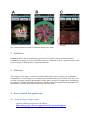
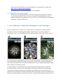
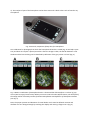
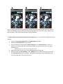
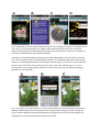
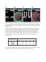
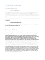
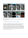
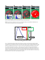
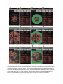
GLAMA – Gap Light Analysis Mobile App
User’s manual
application version 3. 0
Lubomír Tichý
Dept. of Botany and Zoology
Masaryk University
Brno, Czech Republic
1 Introduction
‘Gap Light Analysis Mobile App’ (GLAMA) is a program for calculation of the Canopy
Cover Index estimating canopy cover from hemispherical photographs. The program,
which is freely accessible from the Google Play website, can be used for hemispherical, wideangle and standard photographs (with known lens angle of view). The program was primarily
designed for use in the field, but can also analyse hemispherical photographs saved on
external storage.
Fig. 1: Simple sequence of steps to calculate Canopy Cover Index.
2 Definition
Canopy Cover is the perpendicular projection of tree crowns onto a horizontal surface.
Estimation of canopy cover by visual observation is commonly used in vegetation science and
forest ecology for description of vegetation structure.
3 Efficiency
The Canopy Cover Index is a quick and robust method for precise canopy cover estimation
comparable to visual canopy cover estimation but unaffected by observer bias. Not only can it
be used on already-captured photographs, but the index can also be employed on smartphones
by using the GLAMA Android application to rapidly capture hemispherical photographs and
immediately calculate their index values directly in the field.
4 How to install the application
4.1 Android Operating System
Open the official Google Play web address:
https://play.google.com/store/apps/details?id=com.mobilesglama
and install the program automatically to your device.
Alternatively, the APK file can be downloaded to your smartphone or tablet from:
http://www.sci.muni.cz/botany/glama/
You should run the APK file manually after the download.
4.2 WINDOWS Operating system
If using a PC operating in Windows, this Android application should be installed to
any Android emulator. Of these, I have had experience using BlueStacks, which
supports running the program directly on a PC for a posteriori analysis of photographs
captured by a camera in the field.
5 Lens calibration – definition of hemisphere centre and edges.
Proper calculation of the Canopy Cover Index requires the definition of the hemisphere
perimeter (red circle in following photographs) in pixels. There are three examples of
photographs (Fig. 2), in which different parts of the hemisphere can be taken by the camera.
Fig. 2: Different types of photographs, which can be analysed by GLAMA. Left photograph was taken
with external Nikon Coolpix camera with true fisheye lens and 180° view. Centre photograph was
taken with external fisheye lens used with smartphone built-in camera. Right photograph was simply
taken with built-in smartphone camera.
To my knowledge, it is not possible to take a truly hemispherical photograph (Fig. 2A) with any
smartphone camera at present. Such a photograph can be taken, however, with a professional
camera with an expensive fisheye lens. The analysis of a photograph from such a camera is also
available, but the photograph should first be downloaded to the storage card of the smartphone (see
chapter 6). Fig 2B represents a photograph taken with a smartphone with additional fisheye lens (Fig.
3). The analysis of part of the hemisphere can be done even with a built-in lens such as found in any
smartphone.
Fig. 3: External, inexpensive fisheye lens for smartphone.
Lens calibration for photographs in which the hemispherical border is visible (Fig. 2A and 2B) is quite
easy and does not require a special procedure. After the image is taken, the border between a real
shadow and the lens masking can be identified by definition of the grey colour cut level (Fig. 4).
Fig. 4: Better visualisation of hemisphere border. A horizontal bar below defines a cut level of grey
colour (with a range from 0 to 255). When you move it and select the Refresh button, the dark part of
the image will be covered by red dots for better identification and definition of hemisphere borders
(see Fig. 5).
Next, the proper position and diameter of virtual border circle must be defined. Position and
diameter size are changed simply by touching the display and moving a finger over it (Fig. 5).
Fig. 5: The page with definition of hemisphere borders can be done with a finger. Select the option
“Center” and drag the finger to the centre of the photograph. Then, select the option “Radius” and
drag the finger to the edge of the visible part of the photograph.
If the lens view is so narrow that borders are not visible (Fig. 2C), it is necessary to apply the second
method:
1. Tap on the Question mark button in the Main display (Fig. 6A).
2. Select the Lens calibration button (Fig. 6B).
3. Take a photograph of any circle of known diameter from a known distance. It does not
matter if it is a circle of known size printed on paper or some such ‚circle‘ as a cup, plate,
lampshade, etc.
Note: Record the circle exactly in the photograph’s centre.
4. Define the border and the centre of the photographed circle (Fig. 6C).
5. Write (Fig. 6D) the circle diameter (in cm), distance of the circle from the lens (in cm), and
the lens projection (planar or angular). Recalculate the hemisphere diameter (pixels) and
recommended angle of the horizon mask (°).
Fig. 6: Calibration of narrow-angle (usually built-in) lens of a smartphone camera. It is possible to use
any ‚circle‘, such as a lampshade in your office. After manual definition of the circle centre and
diameter (the program then automatically calculates the circle’s diameter in pixels), it is possible to
calculate a virtual diameter of the whole hemisphere.
Remember or record hemisphere diameter and recommended angle of horizon mask for their next
use in the calculation process. The hemisphere diameter can be defined using either of two display
layouts: 1) In the page with definition of hemisphere borders (Fig. 5), the central ”X” button must be
pressed. The circle will be centred and a query will ask for the circle diameter (Fig. 7); or 2) the
second option is in the page with the definition of the horizon mask (Fig. 8A), where hemisphere
diameter can also be edited.
Fig. 7: The sequence of steps by which to centre a circle, define the virtual hemisphere and define its
diameter. Whereas the circle size and position are wrong in the first image (A), after centring, the
proper diameter definition and proper definition of lens projection at the next screen prepare the
application for correct calculation of the Canopy Cover Index.
Fig. 8: Second option for definition of hemisphere diameter and two alternatives for definition of
horizon masking. Whereas the first two images (A, B) show a simple mask defined by one angle above
the horizon in all directions, the last two images (C, D) show the possibility of individual masking in 16
different directions.
The light incoming from higher zenith angles travels through scattered vegetation, decreasing the
precision of canopy cover estimation. In addition, when conducting a visual assessment of canopy
cover, the observer’s view of the canopy comprises only an upper portion of the sky hemisphere.
Artificial hemisphere masking helps to remove the outer area of a hemispherical photograph,
eliminating some of the light from higher zenith angles. Tab. 1 shows horizon angles, which can be
used for delimitation of a hemispherical photograph depending on the vegetation height and
sampled plot size.
Sample plot size
10 x10m
15 x 15m
20 x 20m
25 x 25m
Maximum height of canopy cover
10m
15m
20m
30m
40m
55°
65°
71°
77°
80°
44°
55°
63°
71°
76°
36°
47°
55°
65°
71°
30°
41°
49°
60°
67°
Tab. 1: Approximate estimated angles of horizon masking for different plot sizes and different heights
of forest canopy when the hemispherical photograph is taken from the plot centre.
6 Paths used by the application
The main path of the application is:
(internal storage)/images
All photographs taken by a built-in camera in JPG format are stored to this path. Their names start
with GLAMA and continue with the date and time of the capture of the photograph. Each
photograph is followed by an .ini file of the same name, which is created during the analysis process.
It saves all selected parameters, and repeated analysis of the photographs can use these pre-defined
values.
Note: All hemispherical photographs taken by a camera not in a smartphone must be copied to this path of internal storage
before the analysis.
The subfolder:
(internal storage)/images/note
contains a global .ini file, which helps with application of all parameters from the last image analysis
to a newly taken hemispherical photograph.
7 Example of field analysis
The process of image analysis in the field starts after selection of the From camera button (Fig. 9A) –
the photograph is then taken (Fig. 9B and 9C). The camera must be held in the horizontal position,
pointed upwards. Most smartphones have a built-in camera both on front and rear side of the
phone. It does not matter which camera will be selected. It is then possible to rotate or flip the taken
photograph (Fig. 9D). On photographs taken with a narrow-angle lens the definition of the
hemispherical border has not relevant (Fig. 9E). Such a function is important, however, when a
fisheye lens is used (Fig. 4 and 5). The hemisphere centre and diameter are usually defined using the
first photograph (Fig. 9F). Also, lens projection is important for correct estimation of the Canopy
Cover Index (Fig. 9G). Lenses of built-in cameras usually have a polar projection (the shortest
distance between two different angles is the same in each part of the photograph), while external
fisheye lenses can have angular projection (the shortest distance between two different angles is
smaller at higher zenith angles). A defined artificial mask (in our example 69°) helps to make the
photograph independent from camera orientation (Fig. 9H), because the photograph uneven width
and height is restricted by a circle with the same distance from its centre. This page also supports a
selection of the level of precision (how many pixels from the photograph will be analysed) and colour
channels (red and blue colours do not penetrate through the vegetation). Final definition of light
gaps (Fig. 9I) depends on the proper selection of a cut level between ‘white’ and ‘black’ pixels. The
final result is presented in the Results page (Fig. 9J).
Fig. 9: Sequence of steps during field image analysis.
Note: Moving between pages is also possible in both directions by moving a finger through the
display to the left or right.
8 Defining cut level between ‘black’ and ‘white’ pixels
The value of this cut level significantly influences the result. Therefore, the application has several
tools for proper identification of shadows made by vegetation and the incoming light from
vegetation gaps. The application calculates a histogram of ‘grey’ colour frequency (the real colour
mix depends on selected channels; Fig. 10A). The cut level is defined from the range 0-255, and the
value automatically recommended corresponds to the intersection of the ideal normal distribution of
‘black’ and the normal distribution of ‘white’ pixels (Fig. 11). The cut level can be modified manually
by moving the horizontal bar at bottom of the layout (Fig. 10B). A single tap to the image will zoom
the area touched by the finger (Fig. 10C). Inverse masking of vegetation by red colour may identify
whether the cut level was selected correctly.
Fig. 10: Tools for definition of cut level between ‘black’ and ‘white’ pixels.
0.8
Note: Every time you change the cut level, use the Refresh button to recalculate it. Otherwise, the
results will be calculated from the last refreshed state.
equal
proportion
of pixels
0.4
0.2
g
0.6
minimum
frequency
black pixels
0.0
white pixels
0
50
100
150
200
250
0:255
Fig. 11: Simulated distribution of pixel colour frequency (in grey scale 0-255) from analysed image.
The image has to be divided into ‘black’ and ‘white’ pixels, which are log-normally distributed over the
gradient. The definition of the correct cut level is the main task influencing estimation precision. We
can estimate the frequency of ‘black’ or ‘white’ pixels as their theoretical log-normal distribution
around some mean value. If the shape of both distributions differs,the modelled equal proportion of
‘black’ and ‘white’ pixels (green line) need not be equal with the minimum frequency over the colour
gradient. The application proposes the cut level between ‘black’ and ‘white’ pixels as an intersectin of
both distributions as the value ‘equal proportion of pixels’.
9
Interpretation of results
Explanation of outputs (Fig. 11):
Total No. of Pixels in Circle (Frame) – The circle defines the virtual border of the hemisphere
(hemisphere horizon) in the photograph. The application estimates the number of pixels within the
whole circle (or hemisphere). In cases, when only part of the whole hemispherical circle is visible on
the page, the number of visible pixels is presented in brackets.
Note: The number of pixels in the circle (frame) is counted independently from the defined mask, which does not influence
the results.
Number of White (Black) Pixels –The real number of white (black) pixels in visible frame.
Note: The number of ‘white’ (‘black’) pixels is limited by the defined mask. All masked ‘white’ pixels are counted as ‘black’.
Gap Fraction of Selected Area – Ratio between ‘white’ and all pixels counted within the visible part
of the circle.
Part of Hemisph. Taken by Camera – It is the percentage ratio of the visible part of the hemisphere.
Canopy Closure –The proportion of the sky hemisphere obscured by canopy elements when viewed
from a single point. Canopy closure is calculated from a hemispherical photograph as the weighted
sum of black pixels as fractions of all pixels within the photograph segements. The weight of these
area fractions is a function of the zenith angle and depends on the camera lens projection (lens
geometric distortion) used.
Canopy Openness – Measure simply complementary to Canopy Closure.
Canopy Cover Index – the main result of hemispherical photograph analysis within this application.
Canopy Cover is the perpendicular projection of tree crowns onto a horizontal surface. Estimation of
canopy cover by visual observation is commonly used in vegetation science and forest ecology for
description of vegetation structure. The Canopy Cover Index can rescale hemispherical projections of
photographs taken from a single position to perpendicular projections of light gaps. Therefore, the
index is suitable to estimate canopy cover directly from hemispherical photographs. It was found that
the index need not be calculated from the fully hemispherical photograph taken by fisheye lenses. If
only the forest vegetation above the plot is analysed (i.e., horizon mask of 45-70°is defined), the
results are more precise.
Selected Colour Cut Level – ASCII value of the colour in a grey scale as the boundary between light
and dark pixels (0-255).
10 Recommended sampling design
Estimation of canopy cover from hemispherical photographs depends on both employing a
satisfactory field sampling strategy to capture representative images, and on proper pixel
classification of the photographs. The field sampling strategy must avoid potential bias in canopy
characterization that can occur due to patchiness of the forest canopy, especially if images are
captured only from openings between trunks. This bias can be avoided by using approaches such as
collecting images from multiple points in transects or grids and averaging their data.
Proper pixel classification is also essential to the accurate use of hemispherical photograph analysis
to quantify canopy cover. The GLAMA software provides a cut-off level between ‘black’ and ‘white’
pixels based on histogram parameterisation and manual visual evaluation of pixel colour differences.
Therefore, you should check every time, to make sure that the cut level is selected properly, i. e. light
gaps are not identified as vegetation nor vice versa.
Fig. 12 shows six different situations – (1) fully hemispherical photograph with no mask; (2) fully
hemispherical photograph with 45° artificial horizon mask; (3) hemispherical photograph with edges
partly out of the page view and no mask; (4) hemispherical photograph with edges partly out of the
layout view and with 45° artificial horizon mas;, (5)partly hemispherical photograph taken by built-in
camera with edges fully out of the page view; and (6) partly hemispherical photograph taken by
built-in camera with edges fully out of the page view and with 69° artificial horizon mask.