1
CHAPTER 5. FEATURE EXTRACTION
156
pi+1
pi
(a)
ωi
pi
pi+1
(b)
ωi+1
ωi+1
(c)
Figure 5.14 Vortex core detection using the combined predictor-corrector/λ2 approach. Starting from a point pi on the vortex core the vorticity ωi is first determined for predicting a new position pi+1 (a) which is then corrected by minimizing λ2 in the plane through pi+1 and perpendicular to ωi+1 (b) to obtain pi+1
from where the next iteration is started using ωi+1 as core direction indicator (c).
Figure inspired by [5].
any vortex tube (including the currently built) in which case the core is terminated and added to the list of detected vortices. If the trace needs to continue
we minimize the λ2 value in the plane defined by vorticity at the predicted position to correct the guess. During this growth process it is very unlikely that a
position—whether predicted or corrected—matches a grid point; thus, interpolation is required. In particular, if we do not want the local minima to be confined
to grid points some higher-order interpolation is required. Therefore, a four-point
Lagrange interpolation as introduced in Section 2.2.2 is utilized (as it is used in
the original implementation). While this interpolation is of high quality, it is also
computationally expensive which presents a major drawback for the minimization
problem since many optimization algorithms are based on the gradient whose determination, in turn, requires several function evaluations. In our application this
translates to prohibitively many Lagrange interpolations and renders traditional
optimization techniques inappropriate. We, therefore, employ a direct search approach [32] which is a brute-force approach not resorting to any analytical aids
like gradients. Instead, the algorithm inspects various neighborhood samples for
guessing a promising direction and then reuses the result to find the most promising direction more quickly in the next iteration. As the method only requires most
basic operations (function evaluations) it has been shown to be robust and to also
work for problems where steepest-decent methods fail.
Once a core vertex has been detected we radially sample the plane perpendicular to the vortex core until a given λ2 threshold is exceeded and encode the
cross section by means of Fourier coefficients as described in Section 2.3.2. Figure 5.15 (b) shows the result of the vortex separation when applying the proposed hybrid vortex detection to the transition data set already used in the previous sections. For the given images, 10 rays where used for sampling the cross