Download OASIS Manual - HydroLogics, Inc.

User Manual
for
OASIS WITH OCL™
model version 3.10.8
gui version 4.6.16
December 1, 2009
Contact Information:
http://www.HydroLogics.net
HydroLogics, Inc.
10440 Shaker Drive, Suite 104
Columbia, MD 21046
410-715-0555
HydroLogics, Inc.
811 Mordecai Drive, Suite 200
Raleigh, NC 27604
919-856-1288
HydroLogics, Inc.
Portland, OR
503-715-9959
Intellectual Property Notice
OASIS with OCL is copyright © 2009 by HydroLogics, Inc.
The Operations Control Language (OCL) is protected by U.S. Patent numbers 6,002,863 and 6,581,027
OASIS makes use of software from the following third parties:
VEDIT is copyright © 1990-2008 by Greenview Data, Inc. (http://www.vedit.com)
XA is copyright © 1993-2008 by Sunset Software Technology. (http://www.sunsetsoft.com)
Microsoft, MS, Microsoft Access, Microsoft Excel, Microsoft FoxPro, MS-DOS, Microsoft W indows, W indows 95,
W indows 98, and W indows XP are registered trademarks of Microsoft Corporation.
Charting Tools for Windows and Real-Time Graphics Tools for Windows are copyright © 1994-2008 by Quinn-Curtis Inc.
(http://www.quinn-curtis.com).
MetaDraw is copyright © 1995-2008 by Bennet-Tec Information Systems, Inc.
(http://www.Bennet-Tec.com).
True DBGrid is a registered trademark of ComponentOne LLC. Copyright © 1995-2008 ComponentOne LLC
(http://www.ComponentOne.com).
-2-
TABLE OF CONTENTS
CHAPTER 1
INTRODUCTION
. . . . . . . . . . . . . . . . . . . . . . . . . . . . . . . . . . . . . . . . . . . . . . . . . . . . . . . . . . . . . . . . . . . . . . . . . . . . . . . . . . . . . . . . . -131.0.0 ORGANIZATION OF THIS MANUAL. . . . . . . . . . . . . . . . . . . . . . . . . . . . . . . . . . . . . . . . . . . . . . . . . . . . . . . . . . . . -131.1.0 OASIS WITH OCL™. . . . . . . . . . . . . . . . . . . . . . . . . . . . . . . . . . . . . . . . . . . . . . . . . . . . . . . . . . . . . . . . . . . . . . . . . . . -131.1.1 LINEAR PROGRAM ROUTING. . . . . . . . . . . . . . . . . . . . . . . . . . . . . . . . . . . . . . . . . . . . . . . . . . . . . . . . . . . . . -131.1.2 OCL. . . . . . . . . . . . . . . . . . . . . . . . . . . . . . . . . . . . . . . . . . . . . . . . . . . . . . . . . . . . . . . . . . . . . . . . . . . . . . . . . . . . -141.1.3 THE ADVANTAGES OF OASIS. . . . . . . . . . . . . . . . . . . . . . . . . . . . . . . . . . . . . . . . . . . . . . . . . . . . . . . . . . . . . -14CHAPTER 2
USER GUIDE. . . . . . . . . . . . . . . . . . . . . . . . . . . . . . . . . . . . . . . . . . . . . . . . . . . . . . . . . . . . . . . . . . . . . . . . . . . . . -162.0.0 INTRODUCTION. . . . . . . . . . . . . . . . . . . . . . . . . . . . . . . . . . . . . . . . . . . . . . . . . . . . . . . . . . . . . . . . . . . . . . . . . . . . . . -162.1.0 REPRESENTATION OF THE PHYSICAL SYSTEM.. . . . . . . . . . . . . . . . . . . . . . . . . . . . . . . . . . . . . . . . . . . . . . . . -162.1.1 NODES.. . . . . . . . . . . . . . . . . . . . . . . . . . . . . . . . . . . . . . . . . . . . . . . . . . . . . . . . . . . . . . . . . . . . . . . . . . . . . . . . . -17A. JUNCTION NODES. . . . . . . . . . . . . . . . . . . . . . . . . . . . . . . . . . . . . . . . . . . . . . . . . . . . . . . . . . -17B. RESERVOIR NODES. . . . . . . . . . . . . . . . . . . . . . . . . . . . . . . . . . . . . . . . . . . . . . . . . . . . . . . . . -18C. DEMAND NODES. . . . . . . . . . . . . . . . . . . . . . . . . . . . . . . . . . . . . . . . . . . . . . . . . . . . . . . . . . . -182.1.2 ARCS. . . . . . . . . . . . . . . . . . . . . . . . . . . . . . . . . . . . . . . . . . . . . . . . . . . . . . . . . . . . . . . . . . . . . . . . . . . . . . . . . . . -182.1.3 INFLOW.. . . . . . . . . . . . . . . . . . . . . . . . . . . . . . . . . . . . . . . . . . . . . . . . . . . . . . . . . . . . . . . . . . . . . . . . . . . . . . . . -192.1.4 TERMINAL NODES. . . . . . . . . . . . . . . . . . . . . . . . . . . . . . . . . . . . . . . . . . . . . . . . . . . . . . . . . . . . . . . . . . . . . . . -192.2.0 DECIDING HOW WATER IS ROUTED. . . . . . . . . . . . . . . . . . . . . . . . . . . . . . . . . . . . . . . . . . . . . . . . . . . . . . . . . . . -202.2.1 DECISION VARIABLES. . . . . . . . . . . . . . . . . . . . . . . . . . . . . . . . . . . . . . . . . . . . . . . . . . . . . . . . . . . . . . . . . . . -202.2.2 OPERATING CONSTRAINTS. . . . . . . . . . . . . . . . . . . . . . . . . . . . . . . . . . . . . . . . . . . . . . . . . . . . . . . . . . . . . . . -212.2.3 OPERATING GOALS AND WEIGHTS. . . . . . . . . . . . . . . . . . . . . . . . . . . . . . . . . . . . . . . . . . . . . . . . . . . . . . . . -212.2.4 CONTINUITY-OF-FLOW CONSTRAINTS.. . . . . . . . . . . . . . . . . . . . . . . . . . . . . . . . . . . . . . . . . . . . . . . . . . . . -232.2.5 ALTERNATE OPTIMA.. . . . . . . . . . . . . . . . . . . . . . . . . . . . . . . . . . . . . . . . . . . . . . . . . . . . . . . . . . . . . . . . . . . . -242.2.6 PRIORITY LEVELS. . . . . . . . . . . . . . . . . . . . . . . . . . . . . . . . . . . . . . . . . . . . . . . . . . . . . . . . . . . . . . . . . . . . . . . -252.2.7 MULTIPLE-PERIOD OPTIMIZATION (MPO). . . . . . . . . . . . . . . . . . . . . . . . . . . . . . . . . . . . . . . . . . . . . . . . . . -262.3.0 MODEL INPUT. . . . . . . . . . . . . . . . . . . . . . . . . . . . . . . . . . . . . . . . . . . . . . . . . . . . . . . . . . . . . . . . . . . . . . . . . . . . . . . . -292.3.1 RUN DIRECTORY. . . . . . . . . . . . . . . . . . . . . . . . . . . . . . . . . . . . . . . . . . . . . . . . . . . . . . . . . . . . . . . . . . . . . . . . -292.3.2 FILES THAT OASIS READS. . . . . . . . . . . . . . . . . . . . . . . . . . . . . . . . . . . . . . . . . . . . . . . . . . . . . . . . . . . . . . . . -302.4.0 STANDARD OPERATING RULES.. . . . . . . . . . . . . . . . . . . . . . . . . . . . . . . . . . . . . . . . . . . . . . . . . . . . . . . . . . . . . . . -31A. MAXIMUM FLOW IN AN ARC. . . . . . . . . . . . . . . . . . . . . . . . . . . . . . . . . . . . . . . . . . . . . . . . -31B. MINIMUM (TARGET) FLOW IN AN ARC. . . . . . . . . . . . . . . . . . . . . . . . . . . . . . . . . . . . . . . -31C. MAXIMUM REVERSE FLOW IN AN ARC. . . . . . . . . . . . . . . . . . . . . . . . . . . . . . . . . . . . . . . -32D. DEMAND AND DELIVERY. . . . . . . . . . . . . . . . . . . . . . . . . . . . . . . . . . . . . . . . . . . . . . . . . . . -33E. INFLOW . . . . . . . . . . . . . . . . . . . . . . . . . . . . . . . . . . . . . . . . . . . . . . . . . . . . . . . . . . . . . . . . . . . -34F. RESERVOIR ELEVATION AND SURFACE AREA. . . . . . . . . . . . . . . . . . . . . . . . . . . . . . . . -34G. RESERVOIR EVAPORATION. . . . . . . . . . . . . . . . . . . . . . . . . . . . . . . . . . . . . . . . . . . . . . . . . -35H. RESERVOIR OPERATIONAL ZONES OR RULE CURVES. . . . . . . . . . . . . . . . . . . . . . . . . -36-
-3-
2.5.0 OPERATIONS CONTROL LANGUAGE (OCL).. . . . . . . . . . . . . . . . . . . . . . . . . . . . . . . . . . . . . . . . . . . . . . . . . . . . -382.5.1 USING OCL SIMULATION COMMANDS. . . . . . . . . . . . . . . . . . . . . . . . . . . . . . . . . . . . . . . . . . . . . . . . . . . . . -39A. Udef command. . . . . . . . . . . . . . . . . . . . . . . . . . . . . . . . . . . . . . . . . . . . . . . . . . . . . . . . . . . . . . . -39B. Segment command. . . . . . . . . . . . . . . . . . . . . . . . . . . . . . . . . . . . . . . . . . . . . . . . . . . . . . . . . . . . -40C. Set command. . . . . . . . . . . . . . . . . . . . . . . . . . . . . . . . . . . . . . . . . . . . . . . . . . . . . . . . . . . . . . . . -40D. Constraint command. . . . . . . . . . . . . . . . . . . . . . . . . . . . . . . . . . . . . . . . . . . . . . . . . . . . . . . . . . -41E. Target command. . . . . . . . . . . . . . . . . . . . . . . . . . . . . . . . . . . . . . . . . . . . . . . . . . . . . . . . . . . . . -42F. Minimax command. . . . . . . . . . . . . . . . . . . . . . . . . . . . . . . . . . . . . . . . . . . . . . . . . . . . . . . . . . . . -43G. Solve command. . . . . . . . . . . . . . . . . . . . . . . . . . . . . . . . . . . . . . . . . . . . . . . . . . . . . . . . . . . . . . -43H. Cancel command. . . . . . . . . . . . . . . . . . . . . . . . . . . . . . . . . . . . . . . . . . . . . . . . . . . . . . . . . . . . . -44I. Run_module command. . . . . . . . . . . . . . . . . . . . . . . . . . . . . . . . . . . . . . . . . . . . . . . . . . . . . . . . . -452.5.2 RETURN FLOW FROM A DEMAND NODE. . . . . . . . . . . . . . . . . . . . . . . . . . . . . . . . . . . . . . . . . . . . . . . . . . . -452.6.0 OUTPUT. . . . . . . . . . . . . . . . . . . . . . . . . . . . . . . . . . . . . . . . . . . . . . . . . . . . . . . . . . . . . . . . . . . . . . . . . . . . . . . . . . . . . . -462.7.0 POST-PROCESSING. . . . . . . . . . . . . . . . . . . . . . . . . . . . . . . . . . . . . . . . . . . . . . . . . . . . . . . . . . . . . . . . . . . . . . . . . . . -472.8.0 TIME IN THE SIMULATION. . . . . . . . . . . . . . . . . . . . . . . . . . . . . . . . . . . . . . . . . . . . . . . . . . . . . . . . . . . . . . . . . . . . -472.8.1 TIME STEPS AND THE TIME CYCLE. . . . . . . . . . . . . . . . . . . . . . . . . . . . . . . . . . . . . . . . . . . . . . . . . . . . . . . . -472.8.2 START AND END. . . . . . . . . . . . . . . . . . . . . . . . . . . . . . . . . . . . . . . . . . . . . . . . . . . . . . . . . . . . . . . . . . . . . . . . . -492.8.3 CONTINUATION MODE. . . . . . . . . . . . . . . . . . . . . . . . . . . . . . . . . . . . . . . . . . . . . . . . . . . . . . . . . . . . . . . . . . . -492.8.4 LEAP YEAR. . . . . . . . . . . . . . . . . . . . . . . . . . . . . . . . . . . . . . . . . . . . . . . . . . . . . . . . . . . . . . . . . . . . . . . . . . . . . -502.8.5 YEAR SCHEME. . . . . . . . . . . . . . . . . . . . . . . . . . . . . . . . . . . . . . . . . . . . . . . . . . . . . . . . . . . . . . . . . . . . . . . . . . -502.9.0 UNITS OF MEASUREMENT.. . . . . . . . . . . . . . . . . . . . . . . . . . . . . . . . . . . . . . . . . . . . . . . . . . . . . . . . . . . . . . . . . . . . -522.10.0 WATER QUALITY. . . . . . . . . . . . . . . . . . . . . . . . . . . . . . . . . . . . . . . . . . . . . . . . . . . . . . . . . . . . . . . . . . . . . . . . . . . . -542.10.1 WATER QUALITY BOUNDARY CONDITIONS. . . . . . . . . . . . . . . . . . . . . . . . . . . . . . . . . . . . . . . . . . . . . . . -552.10.2 WATER QUALITY AT RESERVOIR NODES. . . . . . . . . . . . . . . . . . . . . . . . . . . . . . . . . . . . . . . . . . . . . . . . . -562.10.3 WATER QUALITY OUTPUT. . . . . . . . . . . . . . . . . . . . . . . . . . . . . . . . . . . . . . . . . . . . . . . . . . . . . . . . . . . . . . . -57CHAPTER 3
REFERENCE: GRAPHICAL USER INTERFACE.. . . . . . . . . . . . . . . . . . . . . . . . . . . . . . . . . . . . . . . . . . . . . -583.0.0 INTRODUCTION. . . . . . . . . . . . . . . . . . . . . . . . . . . . . . . . . . . . . . . . . . . . . . . . . . . . . . . . . . . . . . . . . . . . . . . . . . . . . . -583.1.0 INSTALLATION. . . . . . . . . . . . . . . . . . . . . . . . . . . . . . . . . . . . . . . . . . . . . . . . . . . . . . . . . . . . . . . . . . . . . . . . . . . . . . . -583.1.1 UNINSTALLATION. . . . . . . . . . . . . . . . . . . . . . . . . . . . . . . . . . . . . . . . . . . . . . . . . . . . . . . . . . . . . . . . . . . . . . . -593.1.2 COMPONENTS OF THE INSTALLATION PACKAGE. . . . . . . . . . . . . . . . . . . . . . . . . . . . . . . . . . . . . . . . . . . -603.2.0 VEDIT. . . . . . . . . . . . . . . . . . . . . . . . . . . . . . . . . . . . . . . . . . . . . . . . . . . . . . . . . . . . . . . . . . . . . . . . . . . . . . . . . . . . . . . . -603.3.0 FILES AND DIRECTORY STRUCTURE. . . . . . . . . . . . . . . . . . . . . . . . . . . . . . . . . . . . . . . . . . . . . . . . . . . . . . . . . . -613.3.1 STANDARD DIRECTORY STRUCTURE. . . . . . . . . . . . . . . . . . . . . . . . . . . . . . . . . . . . . . . . . . . . . . . . . . . . . . -613.3.2 HOME FOLDER. . . . . . . . . . . . . . . . . . . . . . . . . . . . . . . . . . . . . . . . . . . . . . . . . . . . . . . . . . . . . . . . . . . . . . . . . . -623.3.3 EXECUTABLES FOLDER. . . . . . . . . . . . . . . . . . . . . . . . . . . . . . . . . . . . . . . . . . . . . . . . . . . . . . . . . . . . . . . . . . -633.3.4 POINTER FILE Directry.nam. . . . . . . . . . . . . . . . . . . . . . . . . . . . . . . . . . . . . . . . . . . . . . . . . . . . . . . . . . . . . . . . -643.3.5 CONFIGURATION FILE GUI.ini. . . . . . . . . . . . . . . . . . . . . . . . . . . . . . . . . . . . . . . . . . . . . . . . . . . . . . . . . . . . . -653.3.6 DETERMINING FILE VERSION. . . . . . . . . . . . . . . . . . . . . . . . . . . . . . . . . . . . . . . . . . . . . . . . . . . . . . . . . . . . . -683.3.7 FILES IN THE RUN DIRECTORY.. . . . . . . . . . . . . . . . . . . . . . . . . . . . . . . . . . . . . . . . . . . . . . . . . . . . . . . . . . . -693.3.8 SUBGROUPS.. . . . . . . . . . . . . . . . . . . . . . . . . . . . . . . . . . . . . . . . . . . . . . . . . . . . . . . . . . . . . . . . . . . . . . . . . . . . -70-
-4-
3.4.0 HANDLING RUN DIRECTORIES. . . . . . . . . . . . . . . . . . . . . . . . . . . . . . . . . . . . . . . . . . . . . . . . . . . . . . . . . . . . . . . . -723.4.1 OPEN RUN. . . . . . . . . . . . . . . . . . . . . . . . . . . . . . . . . . . . . . . . . . . . . . . . . . . . . . . . . . . . . . . . . . . . . . . . . . . . . . -723.4.2 CREATING A NEW RUN. . . . . . . . . . . . . . . . . . . . . . . . . . . . . . . . . . . . . . . . . . . . . . . . . . . . . . . . . . . . . . . . . . . -723.4.3 DELETING A RUN. . . . . . . . . . . . . . . . . . . . . . . . . . . . . . . . . . . . . . . . . . . . . . . . . . . . . . . . . . . . . . . . . . . . . . . . -723.4.4 CHANGING THE NAME OF A RUN.. . . . . . . . . . . . . . . . . . . . . . . . . . . . . . . . . . . . . . . . . . . . . . . . . . . . . . . . . -733.4.5 NOTES FILE. . . . . . . . . . . . . . . . . . . . . . . . . . . . . . . . . . . . . . . . . . . . . . . . . . . . . . . . . . . . . . . . . . . . . . . . . . . . . -733.4.6 SAVING THE RUN. . . . . . . . . . . . . . . . . . . . . . . . . . . . . . . . . . . . . . . . . . . . . . . . . . . . . . . . . . . . . . . . . . . . . . . . -733.4.7 SIMULATION MODE AND POSITION-ANALYSIS MODE. . . . . . . . . . . . . . . . . . . . . . . . . . . . . . . . . . . . . . . -743.4.8 RUNNING THE MODEL. . . . . . . . . . . . . . . . . . . . . . . . . . . . . . . . . . . . . . . . . . . . . . . . . . . . . . . . . . . . . . . . . . . -753.4.9 LOCKING RUNS.. . . . . . . . . . . . . . . . . . . . . . . . . . . . . . . . . . . . . . . . . . . . . . . . . . . . . . . . . . . . . . . . . . . . . . . . . -753.5.0 VIEWING OUTPUT. . . . . . . . . . . . . . . . . . . . . . . . . . . . . . . . . . . . . . . . . . . . . . . . . . . . . . . . . . . . . . . . . . . . . . . . . . . . -753.6.0 MENU INTERFACE DETAILS. . . . . . . . . . . . . . . . . . . . . . . . . . . . . . . . . . . . . . . . . . . . . . . . . . . . . . . . . . . . . . . . . . . -763.6.1 File MENU.. . . . . . . . . . . . . . . . . . . . . . . . . . . . . . . . . . . . . . . . . . . . . . . . . . . . . . . . . . . . . . . . . . . . . . . . . . . . . . -763.6.2 Edit MENU.. . . . . . . . . . . . . . . . . . . . . . . . . . . . . . . . . . . . . . . . . . . . . . . . . . . . . . . . . . . . . . . . . . . . . . . . . . . . . . -813.6.3 Run MENU.. . . . . . . . . . . . . . . . . . . . . . . . . . . . . . . . . . . . . . . . . . . . . . . . . . . . . . . . . . . . . . . . . . . . . . . . . . . . . . -863.6.4 Output MENU. . . . . . . . . . . . . . . . . . . . . . . . . . . . . . . . . . . . . . . . . . . . . . . . . . . . . . . . . . . . . . . . . . . . . . . . . . . . -873.6.5 Help MENU. . . . . . . . . . . . . . . . . . . . . . . . . . . . . . . . . . . . . . . . . . . . . . . . . . . . . . . . . . . . . . . . . . . . . . . . . . . . . . -943.7.0 MAIN-WINDOW INTERFACE DETAILS.. . . . . . . . . . . . . . . . . . . . . . . . . . . . . . . . . . . . . . . . . . . . . . . . . . . . . . . . . -963.7.1 Schematic TAB.. . . . . . . . . . . . . . . . . . . . . . . . . . . . . . . . . . . . . . . . . . . . . . . . . . . . . . . . . . . . . . . . . . . . . . . . . . . -96A. SCHEMATIC BUTTONS. . . . . . . . . . . . . . . . . . . . . . . . . . . . . . . . . . . . . . . . . . . . . . . . . . . . . . -96B. NODE AND ARC CATEGORIES AND THE KEYBAR CONTROL. . . . . . . . . . . . . . . . . . . . -98C. SPECIFIC SCHEMATIC TASKS. . . . . . . . . . . . . . . . . . . . . . . . . . . . . . . . . . . . . . . . . . . . . . . . -993.7.2 Setup TAB. . . . . . . . . . . . . . . . . . . . . . . . . . . . . . . . . . . . . . . . . . . . . . . . . . . . . . . . . . . . . . . . . . . . . . . . . . . . . . -103A. TIME RANGE OF RUN. . . . . . . . . . . . . . . . . . . . . . . . . . . . . . . . . . . . . . . . . . . . . . . . . . . . . . -103B. CONTROL BUTTONS. . . . . . . . . . . . . . . . . . . . . . . . . . . . . . . . . . . . . . . . . . . . . . . . . . . . . . . -103C. OCL FILES. . . . . . . . . . . . . . . . . . . . . . . . . . . . . . . . . . . . . . . . . . . . . . . . . . . . . . . . . . . . . . . . . -103D. INITIAL CONDITIONS. . . . . . . . . . . . . . . . . . . . . . . . . . . . . . . . . . . . . . . . . . . . . . . . . . . . . . -103E. GAMING PARAMETERS. . . . . . . . . . . . . . . . . . . . . . . . . . . . . . . . . . . . . . . . . . . . . . . . . . . . . -104F. CUSTOM FEATURES. . . . . . . . . . . . . . . . . . . . . . . . . . . . . . . . . . . . . . . . . . . . . . . . . . . . . . . . -1053.7.3 Time TAB. . . . . . . . . . . . . . . . . . . . . . . . . . . . . . . . . . . . . . . . . . . . . . . . . . . . . . . . . . . . . . . . . . . . . . . . . . . . . . . -105A. SIMULATION TIME RANGE. . . . . . . . . . . . . . . . . . . . . . . . . . . . . . . . . . . . . . . . . . . . . . . . . -105B. TIME STEPS. . . . . . . . . . . . . . . . . . . . . . . . . . . . . . . . . . . . . . . . . . . . . . . . . . . . . . . . . . . . . . . -105C. POSITION ANALYSIS. . . . . . . . . . . . . . . . . . . . . . . . . . . . . . . . . . . . . . . . . . . . . . . . . . . . . . . -1063.7.4 Node TAB.. . . . . . . . . . . . . . . . . . . . . . . . . . . . . . . . . . . . . . . . . . . . . . . . . . . . . . . . . . . . . . . . . . . . . . . . . . . . . . -1073.7.5 Arc TAB. . . . . . . . . . . . . . . . . . . . . . . . . . . . . . . . . . . . . . . . . . . . . . . . . . . . . . . . . . . . . . . . . . . . . . . . . . . . . . . . -1083.7.6 OCL TAB. . . . . . . . . . . . . . . . . . . . . . . . . . . . . . . . . . . . . . . . . . . . . . . . . . . . . . . . . . . . . . . . . . . . . . . . . . . . . . . -1083.7.7 Misc TAB. . . . . . . . . . . . . . . . . . . . . . . . . . . . . . . . . . . . . . . . . . . . . . . . . . . . . . . . . . . . . . . . . . . . . . . . . . . . . . . -1093.8.0 SPECIAL DIALOG BOXES. . . . . . . . . . . . . . . . . . . . . . . . . . . . . . . . . . . . . . . . . . . . . . . . . . . . . . . . . . . . . . . . . . . . . -1103.8.1 Node Settings Dialog Box.. . . . . . . . . . . . . . . . . . . . . . . . . . . . . . . . . . . . . . . . . . . . . . . . . . . . . . . . . . . . . . . . . . -1103.8.2 Arc Settings Dialog Box. . . . . . . . . . . . . . . . . . . . . . . . . . . . . . . . . . . . . . . . . . . . . . . . . . . . . . . . . . . . . . . . . . . . -1133.8.3 Pattern Dialog Box. . . . . . . . . . . . . . . . . . . . . . . . . . . . . . . . . . . . . . . . . . . . . . . . . . . . . . . . . . . . . . . . . . . . . . . . -1153.8.4 Reservoir Storage-Area-Elevation Dialog Box. . . . . . . . . . . . . . . . . . . . . . . . . . . . . . . . . . . . . . . . . . . . . . . . . . -1183.8.5 OCL Lookup Dialog Box. . . . . . . . . . . . . . . . . . . . . . . . . . . . . . . . . . . . . . . . . . . . . . . . . . . . . . . . . . . . . . . . . . . -1193.9.0 STATUS BAR. . . . . . . . . . . . . . . . . . . . . . . . . . . . . . . . . . . . . . . . . . . . . . . . . . . . . . . . . . . . . . . . . . . . . . . . . . . . . . . . . -121-
-5-
CHAPTER 4
REFERENCE: M ODEL INPUT. . . . . . . . . . . . . . . . . . . . . . . . . . . . . . . . . . . . . . . . . . . . . . . . . . . . . . . . . . . . -1224.1.0 COMMAND LINE. . . . . . . . . . . . . . . . . . . . . . . . . . . . . . . . . . . . . . . . . . . . . . . . . . . . . . . . . . . . . . . . . . . . . . . . . . . . . -1224.2.0 IDENTITY KEY.. . . . . . . . . . . . . . . . . . . . . . . . . . . . . . . . . . . . . . . . . . . . . . . . . . . . . . . . . . . . . . . . . . . . . . . . . . . . . . -1244.3.0 POINTER FILE. . . . . . . . . . . . . . . . . . . . . . . . . . . . . . . . . . . . . . . . . . . . . . . . . . . . . . . . . . . . . . . . . . . . . . . . . . . . . . . -1244.4.0 CONTROL FILE. . . . . . . . . . . . . . . . . . . . . . . . . . . . . . . . . . . . . . . . . . . . . . . . . . . . . . . . . . . . . . . . . . . . . . . . . . . . . . -1254.5.0 STATIC DATABASES. . . . . . . . . . . . . . . . . . . . . . . . . . . . . . . . . . . . . . . . . . . . . . . . . . . . . . . . . . . . . . . . . . . . . . . . . -1284.5.1 CONVENTIONS FOR TIME-PATTERN TABLES. . . . . . . . . . . . . . . . . . . . . . . . . . . . . . . . . . . . . . . . . . . . . . -130A. General. . . . . . . . . . . . . . . . . . . . . . . . . . . . . . . . . . . . . . . . . . . . . . . . . . . . . . . . . . . . . . . . . . . -130B. Leap day in pattern input. . . . . . . . . . . . . . . . . . . . . . . . . . . . . . . . . . . . . . . . . . . . . . . . . . . . . . -132C. Redistributing volume input to volume per time step. . . . . . . . . . . . . . . . . . . . . . . . . . . . . . . . -132D. Redistributing flow-rate input to volume per time step. . . . . . . . . . . . . . . . . . . . . . . . . . . . . . . -133E. Redistributing volume input to volume. . . . . . . . . . . . . . . . . . . . . . . . . . . . . . . . . . . . . . . . . . . -134F. Redistributing concentration input. . . . . . . . . . . . . . . . . . . . . . . . . . . . . . . . . . . . . . . . . . . . . . . -135G. Time-series input. . . . . . . . . . . . . . . . . . . . . . . . . . . . . . . . . . . . . . . . . . . . . . . . . . . . . . . . . . . . -1354.5.2 TIME-PARAMETERS DATABASE FILE. . . . . . . . . . . . . . . . . . . . . . . . . . . . . . . . . . . . . . . . . . . . . . . . . . . . . -136A. Table Range.. . . . . . . . . . . . . . . . . . . . . . . . . . . . . . . . . . . . . . . . . . . . . . . . . . . . . . . . . . . . . . . -136B. Table Run. . . . . . . . . . . . . . . . . . . . . . . . . . . . . . . . . . . . . . . . . . . . . . . . . . . . . . . . . . . . . . . . . . -137C. Table Year scheme. . . . . . . . . . . . . . . . . . . . . . . . . . . . . . . . . . . . . . . . . . . . . . . . . . . . . . . . . . . -137D. Table Steps. . . . . . . . . . . . . . . . . . . . . . . . . . . . . . . . . . . . . . . . . . . . . . . . . . . . . . . . . . . . . . . . -138E. Table DSS Steps. . . . . . . . . . . . . . . . . . . . . . . . . . . . . . . . . . . . . . . . . . . . . . . . . . . . . . . . . . . . . -141F. Table PosAnalysis. . . . . . . . . . . . . . . . . . . . . . . . . . . . . . . . . . . . . . . . . . . . . . . . . . . . . . . . . . . -142G. Table Runtime. . . . . . . . . . . . . . . . . . . . . . . . . . . . . . . . . . . . . . . . . . . . . . . . . . . . . . . . . . . . . . -1434.5.3 SYSTEM DATABASE FILE. . . . . . . . . . . . . . . . . . . . . . . . . . . . . . . . . . . . . . . . . . . . . . . . . . . . . . . . . . . . . . . . -144A. Table Units . . . . . . . . . . . . . . . . . . . . . . . . . . . . . . . . . . . . . . . . . . . . . . . . . . . . . . . . . . . . . . . . -144B. Table Node.. . . . . . . . . . . . . . . . . . . . . . . . . . . . . . . . . . . . . . . . . . . . . . . . . . . . . . . . . . . . . . . . -146C. Table Arc. . . . . . . . . . . . . . . . . . . . . . . . . . . . . . . . . . . . . . . . . . . . . . . . . . . . . . . . . . . . . . . . . . -149D. Table Concentration. . . . . . . . . . . . . . . . . . . . . . . . . . . . . . . . . . . . . . . . . . . . . . . . . . . . . . . . . -152E. Table Minimum Flow. . . . . . . . . . . . . . . . . . . . . . . . . . . . . . . . . . . . . . . . . . . . . . . . . . . . . . . . . -153F. Table Maximum Flow.. . . . . . . . . . . . . . . . . . . . . . . . . . . . . . . . . . . . . . . . . . . . . . . . . . . . . . . . -154G. Table Maximum Reverse Flow. . . . . . . . . . . . . . . . . . . . . . . . . . . . . . . . . . . . . . . . . . . . . . . . . -155H. Table Reservoir. . . . . . . . . . . . . . . . . . . . . . . . . . . . . . . . . . . . . . . . . . . . . . . . . . . . . . . . . . . . . -156I. Table Reservoir Rules . . . . . . . . . . . . . . . . . . . . . . . . . . . . . . . . . . . . . . . . . . . . . . . . . . . . . . . . -158J. Table Reservoir S-A-E . . . . . . . . . . . . . . . . . . . . . . . . . . . . . . . . . . . . . . . . . . . . . . . . . . . . . . . . -159K. Table Evaporation. . . . . . . . . . . . . . . . . . . . . . . . . . . . . . . . . . . . . . . . . . . . . . . . . . . . . . . . . . . -160L. Table Evaporation Pattern.. . . . . . . . . . . . . . . . . . . . . . . . . . . . . . . . . . . . . . . . . . . . . . . . . . . . -161M. Table File ID.. . . . . . . . . . . . . . . . . . . . . . . . . . . . . . . . . . . . . . . . . . . . . . . . . . . . . . . . . . . . . . -162N. Table Balance Sheet Columns. . . . . . . . . . . . . . . . . . . . . . . . . . . . . . . . . . . . . . . . . . . . . . . . . . -163O. Table Balance Sheet Rows.. . . . . . . . . . . . . . . . . . . . . . . . . . . . . . . . . . . . . . . . . . . . . . . . . . . . -164P. Table Declare Timeseries.. . . . . . . . . . . . . . . . . . . . . . . . . . . . . . . . . . . . . . . . . . . . . . . . . . . . . -1664.5.4 DEMAND DATABASE FILE. . . . . . . . . . . . . . . . . . . . . . . . . . . . . . . . . . . . . . . . . . . . . . . . . . . . . . . . . . . . . . . -168A. Table Demand. . . . . . . . . . . . . . . . . . . . . . . . . . . . . . . . . . . . . . . . . . . . . . . . . . . . . . . . . . . . . . -168B. Table Demand Pattern.. . . . . . . . . . . . . . . . . . . . . . . . . . . . . . . . . . . . . . . . . . . . . . . . . . . . . . . -169C. Table File ID. . . . . . . . . . . . . . . . . . . . . . . . . . . . . . . . . . . . . . . . . . . . . . . . . . . . . . . . . . . . . . . -1704.5.5 INFLOW DATABASE FILE. . . . . . . . . . . . . . . . . . . . . . . . . . . . . . . . . . . . . . . . . . . . . . . . . . . . . . . . . . . . . . . . -171A. Table Inflow Pattern. . . . . . . . . . . . . . . . . . . . . . . . . . . . . . . . . . . . . . . . . . . . . . . . . . . . . . . . . -171B. Tables C1 Pattern, C2 Pattern, etc.. . . . . . . . . . . . . . . . . . . . . . . . . . . . . . . . . . . . . . . . . . . . . . -172C. Table File ID. . . . . . . . . . . . . . . . . . . . . . . . . . . . . . . . . . . . . . . . . . . . . . . . . . . . . . . . . . . . . . . -1734.5.6 INITIAL CONDITIONS DATABASE FILE. . . . . . . . . . . . . . . . . . . . . . . . . . . . . . . . . . . . . . . . . . . . . . . . . . . . -174A. Table Initial Condition. . . . . . . . . . . . . . . . . . . . . . . . . . . . . . . . . . . . . . . . . . . . . . . . . . . . . . . -174-
-6-
4.5.7 WEIGHTS DATABASE FILE. . . . . . . . . . . . . . . . . . . . . . . . . . . . . . . . . . . . . . . . . . . . . . . . . . . . . . . . . . . . . . . -175A. Table Weight: Arc. . . . . . . . . . . . . . . . . . . . . . . . . . . . . . . . . . . . . . . . . . . . . . . . . . . . . . . . . . . -175B. Table Weight: Storage. . . . . . . . . . . . . . . . . . . . . . . . . . . . . . . . . . . . . . . . . . . . . . . . . . . . . . . . -176C. Table Weight: Demand . . . . . . . . . . . . . . . . . . . . . . . . . . . . . . . . . . . . . . . . . . . . . . . . . . . . . . . -1774.5.8 OCL STATIC DATABASE FILE. . . . . . . . . . . . . . . . . . . . . . . . . . . . . . . . . . . . . . . . . . . . . . . . . . . . . . . . . . . . -178A. Table Lookup. . . . . . . . . . . . . . . . . . . . . . . . . . . . . . . . . . . . . . . . . . . . . . . . . . . . . . . . . . . . . . . -178B. Table Pattern. . . . . . . . . . . . . . . . . . . . . . . . . . . . . . . . . . . . . . . . . . . . . . . . . . . . . . . . . . . . . . . -1794.5.9 STATIC DATABASE TABLES USED BY THE OASIS GUI. . . . . . . . . . . . . . . . . . . . . . . . . . . . . . . . . . . . . . -181C. Table Constants. . . . . . . . . . . . . . . . . . . . . . . . . . . . . . . . . . . . . . . . . . . . . . . . . . . . . . . . . . . . . -181D. Table zzGUI_Status. . . . . . . . . . . . . . . . . . . . . . . . . . . . . . . . . . . . . . . . . . . . . . . . . . . . . . . . . . -181E. Table zzGUI_Page. . . . . . . . . . . . . . . . . . . . . . . . . . . . . . . . . . . . . . . . . . . . . . . . . . . . . . . . . . . -182F. Table zzGUI_NodeType. . . . . . . . . . . . . . . . . . . . . . . . . . . . . . . . . . . . . . . . . . . . . . . . . . . . . . . -182G. Table zzGUI_ArcType. . . . . . . . . . . . . . . . . . . . . . . . . . . . . . . . . . . . . . . . . . . . . . . . . . . . . . . . -183H. Table zzGUI_InflowType. . . . . . . . . . . . . . . . . . . . . . . . . . . . . . . . . . . . . . . . . . . . . . . . . . . . . . -183I. Table zzGUI_Text. . . . . . . . . . . . . . . . . . . . . . . . . . . . . . . . . . . . . . . . . . . . . . . . . . . . . . . . . . . . -184J. Table zzGUI_Shape. . . . . . . . . . . . . . . . . . . . . . . . . . . . . . . . . . . . . . . . . . . . . . . . . . . . . . . . . . -185K. Table zzGUI_Link. . . . . . . . . . . . . . . . . . . . . . . . . . . . . . . . . . . . . . . . . . . . . . . . . . . . . . . . . . . -187L. Table zzGUI_Image. . . . . . . . . . . . . . . . . . . . . . . . . . . . . . . . . . . . . . . . . . . . . . . . . . . . . . . . . . -188M. Table zzGUI_ZOrder. . . . . . . . . . . . . . . . . . . . . . . . . . . . . . . . . . . . . . . . . . . . . . . . . . . . . . . . -1894.6.0 TIME-SERIES DATABASES. . . . . . . . . . . . . . . . . . . . . . . . . . . . . . . . . . . . . . . . . . . . . . . . . . . . . . . . . . . . . . . . . . . . -1904.6.1 CONVENTIONS IN TIME-SERIES DATABASES. . . . . . . . . . . . . . . . . . . . . . . . . . . . . . . . . . . . . . . . . . . . . . -1904.6.2 SYSTEM TIME-SERIES FILE. . . . . . . . . . . . . . . . . . . . . . . . . . . . . . . . . . . . . . . . . . . . . . . . . . . . . . . . . . . . . . -192A. Time-series minimum flow. . . . . . . . . . . . . . . . . . . . . . . . . . . . . . . . . . . . . . . . . . . . . . . . . . . . -192B. Time-series maximum flow. . . . . . . . . . . . . . . . . . . . . . . . . . . . . . . . . . . . . . . . . . . . . . . . . . . . -192C. Time-series maximum reverse flow. . . . . . . . . . . . . . . . . . . . . . . . . . . . . . . . . . . . . . . . . . . . . . -193D. Time-series reservoir evaporation rate.. . . . . . . . . . . . . . . . . . . . . . . . . . . . . . . . . . . . . . . . . . . -193E. Time-series reservoir upper-rule curve. . . . . . . . . . . . . . . . . . . . . . . . . . . . . . . . . . . . . . . . . . . -193F. Time-series reservoir lower-rule curve.. . . . . . . . . . . . . . . . . . . . . . . . . . . . . . . . . . . . . . . . . . . -1944.6.3 DEMAND TIME-SERIES FILE. . . . . . . . . . . . . . . . . . . . . . . . . . . . . . . . . . . . . . . . . . . . . . . . . . . . . . . . . . . . . -194A. Time-series demand. . . . . . . . . . . . . . . . . . . . . . . . . . . . . . . . . . . . . . . . . . . . . . . . . . . . . . . . . . -1944.6.4 INFLOW TIME-SERIES FILE. . . . . . . . . . . . . . . . . . . . . . . . . . . . . . . . . . . . . . . . . . . . . . . . . . . . . . . . . . . . . . -195A. Time-series inflow. . . . . . . . . . . . . . . . . . . . . . . . . . . . . . . . . . . . . . . . . . . . . . . . . . . . . . . . . . . -195B. Time-series concentration input at a node. . . . . . . . . . . . . . . . . . . . . . . . . . . . . . . . . . . . . . . . . -195C. Time-series concentration input at an arc.. . . . . . . . . . . . . . . . . . . . . . . . . . . . . . . . . . . . . . . . . -1964.6.5 OCL TIME-SERIES FILE. . . . . . . . . . . . . . . . . . . . . . . . . . . . . . . . . . . . . . . . . . . . . . . . . . . . . . . . . . . . . . . . . . -196A. OCL time-series input. . . . . . . . . . . . . . . . . . . . . . . . . . . . . . . . . . . . . . . . . . . . . . . . . . . . . . . . -196-
-7-
4.7.0 OPERATIONS CONTROL LANGUAGE (OCL).. . . . . . . . . . . . . . . . . . . . . . . . . . . . . . . . . . . . . . . . . . . . . . . . . . . -197A. General OCL syntax. . . . . . . . . . . . . . . . . . . . . . . . . . . . . . . . . . . . . . . . . . . . . . . . . . . . . . . . . -197B. Quotation marks.. . . . . . . . . . . . . . . . . . . . . . . . . . . . . . . . . . . . . . . . . . . . . . . . . . . . . . . . . . . . -198C. Square brackets and substitute names. . . . . . . . . . . . . . . . . . . . . . . . . . . . . . . . . . . . . . . . . . . . -198D. Comment markers. . . . . . . . . . . . . . . . . . . . . . . . . . . . . . . . . . . . . . . . . . . . . . . . . . . . . . . . . . . -198E. Simulation commands. . . . . . . . . . . . . . . . . . . . . . . . . . . . . . . . . . . . . . . . . . . . . . . . . . . . . . . . -199F. Meta commands. . . . . . . . . . . . . . . . . . . . . . . . . . . . . . . . . . . . . . . . . . . . . . . . . . . . . . . . . . . . . -199G. Sections of the OCL file. . . . . . . . . . . . . . . . . . . . . . . . . . . . . . . . . . . . . . . . . . . . . . . . . . . . . . -2004.7.1 SYNTAX OF OCL META COMMANDS.. . . . . . . . . . . . . . . . . . . . . . . . . . . . . . . . . . . . . . . . . . . . . . . . . . . . . -200A. :UDEF:. . . . . . . . . . . . . . . . . . . . . . . . . . . . . . . . . . . . . . . . . . . . . . . . . . . . . . . . . . . . . . . . . . . -200B. :COMMANDS:. . . . . . . . . . . . . . . . . . . . . . . . . . . . . . . . . . . . . . . . . . . . . . . . . . . . . . . . . . . . . -200C. :END:. . . . . . . . . . . . . . . . . . . . . . . . . . . . . . . . . . . . . . . . . . . . . . . . . . . . . . . . . . . . . . . . . . . . . -200D. :ITERATE:. . . . . . . . . . . . . . . . . . . . . . . . . . . . . . . . . . . . . . . . . . . . . . . . . . . . . . . . . . . . . . . . -200E. :STATDB:. . . . . . . . . . . . . . . . . . . . . . . . . . . . . . . . . . . . . . . . . . . . . . . . . . . . . . . . . . . . . . . . . -201F. :TIMEDB:. . . . . . . . . . . . . . . . . . . . . . . . . . . . . . . . . . . . . . . . . . . . . . . . . . . . . . . . . . . . . . . . . -201G. :MODULE:. . . . . . . . . . . . . . . . . . . . . . . . . . . . . . . . . . . . . . . . . . . . . . . . . . . . . . . . . . . . . . . . -201H. :INCLUDE:. . . . . . . . . . . . . . . . . . . . . . . . . . . . . . . . . . . . . . . . . . . . . . . . . . . . . . . . . . . . . . . . -201I. :SUBSTITUTE:. . . . . . . . . . . . . . . . . . . . . . . . . . . . . . . . . . . . . . . . . . . . . . . . . . . . . . . . . . . . . -202J. :FOR: :NEXT:. . . . . . . . . . . . . . . . . . . . . . . . . . . . . . . . . . . . . . . . . . . . . . . . . . . . . . . . . . . . . . -203K. :IF: :ELSEIF: :ELSE: :ENDIF:.. . . . . . . . . . . . . . . . . . . . . . . . . . . . . . . . . . . . . . . . . . . . . . . -2044.7.2 SYNTAX OF OCL SIMULATION COMMANDS. . . . . . . . . . . . . . . . . . . . . . . . . . . . . . . . . . . . . . . . . . . . . . . -206A. Conditions. . . . . . . . . . . . . . . . . . . . . . . . . . . . . . . . . . . . . . . . . . . . . . . . . . . . . . . . . . . . . . . . . -206B. Udef Command. . . . . . . . . . . . . . . . . . . . . . . . . . . . . . . . . . . . . . . . . . . . . . . . . . . . . . . . . . . . . -208C. Segment Command. . . . . . . . . . . . . . . . . . . . . . . . . . . . . . . . . . . . . . . . . . . . . . . . . . . . . . . . . . -210D. Constraint Command.. . . . . . . . . . . . . . . . . . . . . . . . . . . . . . . . . . . . . . . . . . . . . . . . . . . . . . . . -211E. Target Command. . . . . . . . . . . . . . . . . . . . . . . . . . . . . . . . . . . . . . . . . . . . . . . . . . . . . . . . . . . . -212F. Set Command. . . . . . . . . . . . . . . . . . . . . . . . . . . . . . . . . . . . . . . . . . . . . . . . . . . . . . . . . . . . . . . -216G. Run_module Command. . . . . . . . . . . . . . . . . . . . . . . . . . . . . . . . . . . . . . . . . . . . . . . . . . . . . . . -218H. Minimax Command. . . . . . . . . . . . . . . . . . . . . . . . . . . . . . . . . . . . . . . . . . . . . . . . . . . . . . . . . . -220I. Solve Command.. . . . . . . . . . . . . . . . . . . . . . . . . . . . . . . . . . . . . . . . . . . . . . . . . . . . . . . . . . . . . -222J. Cancel Command. . . . . . . . . . . . . . . . . . . . . . . . . . . . . . . . . . . . . . . . . . . . . . . . . . . . . . . . . . . . -2254.7.3 SYNTAX OF OCL EXPRESSIONS. . . . . . . . . . . . . . . . . . . . . . . . . . . . . . . . . . . . . . . . . . . . . . . . . . . . . . . . . . -2274.7.4 SYNTAX OF OCL NON-DECISION VARIABLES.. . . . . . . . . . . . . . . . . . . . . . . . . . . . . . . . . . . . . . . . . . . . . -228A. Time lags and time indices on non-decision variables. . . . . . . . . . . . . . . . . . . . . . . . . . . . . . . . -228B. Abs_period variable. . . . . . . . . . . . . . . . . . . . . . . . . . . . . . . . . . . . . . . . . . . . . . . . . . . . . . . . . . -229C. Ann_demand variable. . . . . . . . . . . . . . . . . . . . . . . . . . . . . . . . . . . . . . . . . . . . . . . . . . . . . . . . -229D. Concentration variable. . . . . . . . . . . . . . . . . . . . . . . . . . . . . . . . . . . . . . . . . . . . . . . . . . . . . . . -229E. Conc_input variable at a node. . . . . . . . . . . . . . . . . . . . . . . . . . . . . . . . . . . . . . . . . . . . . . . . . . -229F. Conc_input variable at an arc. . . . . . . . . . . . . . . . . . . . . . . . . . . . . . . . . . . . . . . . . . . . . . . . . . . -229G. Cycle_step variable. . . . . . . . . . . . . . . . . . . . . . . . . . . . . . . . . . . . . . . . . . . . . . . . . . . . . . . . . . -229H. Day variable.. . . . . . . . . . . . . . . . . . . . . . . . . . . . . . . . . . . . . . . . . . . . . . . . . . . . . . . . . . . . . . . -230I. Dead_stor variable. . . . . . . . . . . . . . . . . . . . . . . . . . . . . . . . . . . . . . . . . . . . . . . . . . . . . . . . . . . -230J. Demand variable. . . . . . . . . . . . . . . . . . . . . . . . . . . . . . . . . . . . . . . . . . . . . . . . . . . . . . . . . . . . . -230K. Delivery variable. . . . . . . . . . . . . . . . . . . . . . . . . . . . . . . . . . . . . . . . . . . . . . . . . . . . . . . . . . . . -230L. Elevation variable. . . . . . . . . . . . . . . . . . . . . . . . . . . . . . . . . . . . . . . . . . . . . . . . . . . . . . . . . . . -230M. Evap variable. . . . . . . . . . . . . . . . . . . . . . . . . . . . . . . . . . . . . . . . . . . . . . . . . . . . . . . . . . . . . . -230N. Evap_rate variable.. . . . . . . . . . . . . . . . . . . . . . . . . . . . . . . . . . . . . . . . . . . . . . . . . . . . . . . . . . -230O. Flow variable. . . . . . . . . . . . . . . . . . . . . . . . . . . . . . . . . . . . . . . . . . . . . . . . . . . . . . . . . . . . . . . -231P. Inflow variable. . . . . . . . . . . . . . . . . . . . . . . . . . . . . . . . . . . . . . . . . . . . . . . . . . . . . . . . . . . . . . -231Q. Julian variable. . . . . . . . . . . . . . . . . . . . . . . . . . . . . . . . . . . . . . . . . . . . . . . . . . . . . . . . . . . . . . -231R. Length variable. . . . . . . . . . . . . . . . . . . . . . . . . . . . . . . . . . . . . . . . . . . . . . . . . . . . . . . . . . . . . -231S. Lower_rule variable. . . . . . . . . . . . . . . . . . . . . . . . . . . . . . . . . . . . . . . . . . . . . . . . . . . . . . . . . . -231T. Max_flow variable. . . . . . . . . . . . . . . . . . . . . . . . . . . . . . . . . . . . . . . . . . . . . . . . . . . . . . . . . . . -231U. Max_stor variable. . . . . . . . . . . . . . . . . . . . . . . . . . . . . . . . . . . . . . . . . . . . . . . . . . . . . . . . . . . -231V. MaxRev_flow variable. . . . . . . . . . . . . . . . . . . . . . . . . . . . . . . . . . . . . . . . . . . . . . . . . . . . . . . . -232-
-8-
W . Min_flow variable. . . . . . . . . . . . . . . . . . . . . . . . . . . . . . . . . . . . . . . . . . . . . . . . . . . . . . . . . . .
X. Minute variable. . . . . . . . . . . . . . . . . . . . . . . . . . . . . . . . . . . . . . . . . . . . . . . . . . . . . . . . . . . . .
Y. Month variable. . . . . . . . . . . . . . . . . . . . . . . . . . . . . . . . . . . . . . . . . . . . . . . . . . . . . . . . . . . . . .
Z. MPO_step variable.. . . . . . . . . . . . . . . . . . . . . . . . . . . . . . . . . . . . . . . . . . . . . . . . . . . . . . . . . .
AA. Num_MPO_steps variable. . . . . . . . . . . . . . . . . . . . . . . . . . . . . . . . . . . . . . . . . . . . . . . . . . .
BB. Pattern variable. . . . . . . . . . . . . . . . . . . . . . . . . . . . . . . . . . . . . . . . . . . . . . . . . . . . . . . . . . . .
CC. Period variable. . . . . . . . . . . . . . . . . . . . . . . . . . . . . . . . . . . . . . . . . . . . . . . . . . . . . . . . . . . .
DD. Prep variable.. . . . . . . . . . . . . . . . . . . . . . . . . . . . . . . . . . . . . . . . . . . . . . . . . . . . . . . . . . . . .
EE. Shortage variable. . . . . . . . . . . . . . . . . . . . . . . . . . . . . . . . . . . . . . . . . . . . . . . . . . . . . . . . . . .
FF. Storage variable. . . . . . . . . . . . . . . . . . . . . . . . . . . . . . . . . . . . . . . . . . . . . . . . . . . . . . . . . . . .
GG. Table variable. . . . . . . . . . . . . . . . . . . . . . . . . . . . . . . . . . . . . . . . . . . . . . . . . . . . . . . . . . . . .
HH. Target_val variable. . . . . . . . . . . . . . . . . . . . . . . . . . . . . . . . . . . . . . . . . . . . . . . . . . . . . . . . .
II. Timesers variable. . . . . . . . . . . . . . . . . . . . . . . . . . . . . . . . . . . . . . . . . . . . . . . . . . . . . . . . . . . .
JJ. Upper_rule variable. . . . . . . . . . . . . . . . . . . . . . . . . . . . . . . . . . . . . . . . . . . . . . . . . . . . . . . . .
KK. Year variable. . . . . . . . . . . . . . . . . . . . . . . . . . . . . . . . . . . . . . . . . . . . . . . . . . . . . . . . . . . . . .
LL. Udef variable. . . . . . . . . . . . . . . . . . . . . . . . . . . . . . . . . . . . . . . . . . . . . . . . . . . . . . . . . . . . . .
-232-232-232-232-232-232-233-233-233-233-233-233-234-234-234-234-
4.7.5 SYNTAX OF OCL DECISION VARIABLES.. . . . . . . . . . . . . . . . . . . . . . . . . . . . . . . . . . . . . . . . . . . . . . . . . . -235A. Time lags on decision variables. . . . . . . . . . . . . . . . . . . . . . . . . . . . . . . . . . . . . . . . . . . . . . . . . -235B. dDelivery variable. . . . . . . . . . . . . . . . . . . . . . . . . . . . . . . . . . . . . . . . . . . . . . . . . . . . . . . . . . . -236C. dFlow variable. . . . . . . . . . . . . . . . . . . . . . . . . . . . . . . . . . . . . . . . . . . . . . . . . . . . . . . . . . . . . . -236D. Flow-split variables. . . . . . . . . . . . . . . . . . . . . . . . . . . . . . . . . . . . . . . . . . . . . . . . . . . . . . . . . . -236E. dStorage variable. . . . . . . . . . . . . . . . . . . . . . . . . . . . . . . . . . . . . . . . . . . . . . . . . . . . . . . . . . . . -236F. Storage zone variables. . . . . . . . . . . . . . . . . . . . . . . . . . . . . . . . . . . . . . . . . . . . . . . . . . . . . . . . -236G. Udef decision variables. . . . . . . . . . . . . . . . . . . . . . . . . . . . . . . . . . . . . . . . . . . . . . . . . . . . . . . -2374.7.6 SYNTAX OF OCL FUNCTIONS. . . . . . . . . . . . . . . . . . . . . . . . . . . . . . . . . . . . . . . . . . . . . . . . . . . . . . . . . . . . -238A. Abs_val function. . . . . . . . . . . . . . . . . . . . . . . . . . . . . . . . . . . . . . . . . . . . . . . . . . . . . . . . . . . . -238B. Accumulate function. . . . . . . . . . . . . . . . . . . . . . . . . . . . . . . . . . . . . . . . . . . . . . . . . . . . . . . . . -238C. Convert_units function.. . . . . . . . . . . . . . . . . . . . . . . . . . . . . . . . . . . . . . . . . . . . . . . . . . . . . . . -238D. Date_to_Jul function. . . . . . . . . . . . . . . . . . . . . . . . . . . . . . . . . . . . . . . . . . . . . . . . . . . . . . . . . -239E. Elev_to_stor function. . . . . . . . . . . . . . . . . . . . . . . . . . . . . . . . . . . . . . . . . . . . . . . . . . . . . . . . . -239F. Exp function. . . . . . . . . . . . . . . . . . . . . . . . . . . . . . . . . . . . . . . . . . . . . . . . . . . . . . . . . . . . . . . . -239G. Floor function. . . . . . . . . . . . . . . . . . . . . . . . . . . . . . . . . . . . . . . . . . . . . . . . . . . . . . . . . . . . . . -239H. Is_Leap_Year function.. . . . . . . . . . . . . . . . . . . . . . . . . . . . . . . . . . . . . . . . . . . . . . . . . . . . . . . -239I. Jul_to_Day function. . . . . . . . . . . . . . . . . . . . . . . . . . . . . . . . . . . . . . . . . . . . . . . . . . . . . . . . . . -239J. Jul_to_Month function. . . . . . . . . . . . . . . . . . . . . . . . . . . . . . . . . . . . . . . . . . . . . . . . . . . . . . . . -240K. Log10 function.. . . . . . . . . . . . . . . . . . . . . . . . . . . . . . . . . . . . . . . . . . . . . . . . . . . . . . . . . . . . . -240L. LogN function.. . . . . . . . . . . . . . . . . . . . . . . . . . . . . . . . . . . . . . . . . . . . . . . . . . . . . . . . . . . . . . -240M. Lookup function. . . . . . . . . . . . . . . . . . . . . . . . . . . . . . . . . . . . . . . . . . . . . . . . . . . . . . . . . . . . -240N. Max function. . . . . . . . . . . . . . . . . . . . . . . . . . . . . . . . . . . . . . . . . . . . . . . . . . . . . . . . . . . . . . . -240O. Min function. . . . . . . . . . . . . . . . . . . . . . . . . . . . . . . . . . . . . . . . . . . . . . . . . . . . . . . . . . . . . . . -240P. Remainder function. . . . . . . . . . . . . . . . . . . . . . . . . . . . . . . . . . . . . . . . . . . . . . . . . . . . . . . . . . -240Q. RevLookup function. . . . . . . . . . . . . . . . . . . . . . . . . . . . . . . . . . . . . . . . . . . . . . . . . . . . . . . . . . -240R. Round function.. . . . . . . . . . . . . . . . . . . . . . . . . . . . . . . . . . . . . . . . . . . . . . . . . . . . . . . . . . . . . -241S. Stor_to_area function.. . . . . . . . . . . . . . . . . . . . . . . . . . . . . . . . . . . . . . . . . . . . . . . . . . . . . . . . -241T. Stor_to_elev function. . . . . . . . . . . . . . . . . . . . . . . . . . . . . . . . . . . . . . . . . . . . . . . . . . . . . . . . . -241U. TimeAccum function. . . . . . . . . . . . . . . . . . . . . . . . . . . . . . . . . . . . . . . . . . . . . . . . . . . . . . . . . -241V. TimeOffset function. . . . . . . . . . . . . . . . . . . . . . . . . . . . . . . . . . . . . . . . . . . . . . . . . . . . . . . . . . -243W . Weekday function. . . . . . . . . . . . . . . . . . . . . . . . . . . . . . . . . . . . . . . . . . . . . . . . . . . . . . . . . . . -2454.7.7 EXTERNAL MODULES. . . . . . . . . . . . . . . . . . . . . . . . . . . . . . . . . . . . . . . . . . . . . . . . . . . . . . . . . . . . . . . . . . . -246A. General steps of the external module protocol.. . . . . . . . . . . . . . . . . . . . . . . . . . . . . . . . . . . . . -246B. Dynamic Link Library (DLL). . . . . . . . . . . . . . . . . . . . . . . . . . . . . . . . . . . . . . . . . . . . . . . . . . -247C. Parent module. . . . . . . . . . . . . . . . . . . . . . . . . . . . . . . . . . . . . . . . . . . . . . . . . . . . . . . . . . . . . . -248-
-9-
CHAPTER 5
REFERENCE: M ODEL OUTPUT. . . . . . . . . . . . . . . . . . . . . . . . . . . . . . . . . . . . . . . . . . . . . . . . . . . . . . . . . . -2495.0.0 INTRODUCTION. . . . . . . . . . . . . . . . . . . . . . . . . . . . . . . . . . . . . . . . . . . . . . . . . . . . . . . . . . . . . . . . . . . . . . . . . . . . . -2495.1.0 DEBUG OUTPUT. . . . . . . . . . . . . . . . . . . . . . . . . . . . . . . . . . . . . . . . . . . . . . . . . . . . . . . . . . . . . . . . . . . . . . . . . . . . . -2495.2.0 BALANCE SHEET OUTPUT.. . . . . . . . . . . . . . . . . . . . . . . . . . . . . . . . . . . . . . . . . . . . . . . . . . . . . . . . . . . . . . . . . . . -2505.3.0 OCL OUTPUT. . . . . . . . . . . . . . . . . . . . . . . . . . . . . . . . . . . . . . . . . . . . . . . . . . . . . . . . . . . . . . . . . . . . . . . . . . . . . . . . -2515.3.1 SUMMARY OF OCL INPUT. . . . . . . . . . . . . . . . . . . . . . . . . . . . . . . . . . . . . . . . . . . . . . . . . . . . . . . . . . . . . . . -2515.3.2 OCL EXPRESSION RESULTS. . . . . . . . . . . . . . . . . . . . . . . . . . . . . . . . . . . . . . . . . . . . . . . . . . . . . . . . . . . . . . -2515.3.3 REPORT OF TARGET AND MINIMAX RESULTS. . . . . . . . . . . . . . . . . . . . . . . . . . . . . . . . . . . . . . . . . . . . . -2535.4.0 WEIGHT OUTPUT. . . . . . . . . . . . . . . . . . . . . . . . . . . . . . . . . . . . . . . . . . . . . . . . . . . . . . . . . . . . . . . . . . . . . . . . . . . . -2535.5.0 LP OUTPUT. . . . . . . . . . . . . . . . . . . . . . . . . . . . . . . . . . . . . . . . . . . . . . . . . . . . . . . . . . . . . . . . . . . . . . . . . . . . . . . . . . -2535.5.1 STATEMENT OF THE LP. . . . . . . . . . . . . . . . . . . . . . . . . . . . . . . . . . . . . . . . . . . . . . . . . . . . . . . . . . . . . . . . . -2545.5.2 LP SOLUTION REPORT. . . . . . . . . . . . . . . . . . . . . . . . . . . . . . . . . . . . . . . . . . . . . . . . . . . . . . . . . . . . . . . . . . -2555.6.0 TIME-SERIES OUTPUT. . . . . . . . . . . . . . . . . . . . . . . . . . . . . . . . . . . . . . . . . . . . . . . . . . . . . . . . . . . . . . . . . . . . . . . -256CHAPTER 6
REFERENCE: POST-PROCESSOR PROGRAM S.. . . . . . . . . . . . . . . . . . . . . . . . . . . . . . . . . . . . . . . . . . . . -2586.0.0 INTRODUCTION. . . . . . . . . . . . . . . . . . . . . . . . . . . . . . . . . . . . . . . . . . . . . . . . . . . . . . . . . . . . . . . . . . . . . . . . . . . . . -2586.1.0 ONEVAR PROGRAM.. . . . . . . . . . . . . . . . . . . . . . . . . . . . . . . . . . . . . . . . . . . . . . . . . . . . . . . . . . . . . . . . . . . . . . . . . -2586.1.1 ONEVAR COMPUTATIONS. . . . . . . . . . . . . . . . . . . . . . . . . . . . . . . . . . . . . . . . . . . . . . . . . . . . . . . . . . . . . . . -2596.1.2 ONEVAR POINTER FILE. . . . . . . . . . . . . . . . . . . . . . . . . . . . . . . . . . . . . . . . . . . . . . . . . . . . . . . . . . . . . . . . . -2606.1.3 ONEVAR INPUT FILE. . . . . . . . . . . . . . . . . . . . . . . . . . . . . . . . . . . . . . . . . . . . . . . . . . . . . . . . . . . . . . . . . . . . -2606.1.4 FORMATS OF THE ONEVAR OUTPUT FILE. . . . . . . . . . . . . . . . . . . . . . . . . . . . . . . . . . . . . . . . . . . . . . . . . -262A. TABLE format type. . . . . . . . . . . . . . . . . . . . . . . . . . . . . . . . . . . . . . . . . . . . . . . . . . . . . . . . . . -262B. COLUMN format type. . . . . . . . . . . . . . . . . . . . . . . . . . . . . . . . . . . . . . . . . . . . . . . . . . . . . . . . -264C. SEQUENTIAL format type.. . . . . . . . . . . . . . . . . . . . . . . . . . . . . . . . . . . . . . . . . . . . . . . . . . . . -266D. REPORT format type. . . . . . . . . . . . . . . . . . . . . . . . . . . . . . . . . . . . . . . . . . . . . . . . . . . . . . . . . -2686.1.5 HEC-DSS OUTPUT FROM ONEVAR. . . . . . . . . . . . . . . . . . . . . . . . . . . . . . . . . . . . . . . . . . . . . . . . . . . . . . . . -2716.1.6 USING ONEVAR AS A PRE-PROCESSOR. . . . . . . . . . . . . . . . . . . . . . . . . . . . . . . . . . . . . . . . . . . . . . . . . . . -2716.1.7 FIELDS OF THE ONEVAR INPUT-FILE HEADER SECTION. . . . . . . . . . . . . . . . . . . . . . . . . . . . . . . . . . . . -273A. :FILE: field. . . . . . . . . . . . . . . . . . . . . . . . . . . . . . . . . . . . . . . . . . . . . . . . . . . . . . . . . . . . . . . . -273B. :FILEDSS: field. . . . . . . . . . . . . . . . . . . . . . . . . . . . . . . . . . . . . . . . . . . . . . . . . . . . . . . . . . . . . -273C. :FILEIHB: field. . . . . . . . . . . . . . . . . . . . . . . . . . . . . . . . . . . . . . . . . . . . . . . . . . . . . . . . . . . . . -273D. :STATDB: field. . . . . . . . . . . . . . . . . . . . . . . . . . . . . . . . . . . . . . . . . . . . . . . . . . . . . . . . . . . . . -274E. :TIMEDB: field. . . . . . . . . . . . . . . . . . . . . . . . . . . . . . . . . . . . . . . . . . . . . . . . . . . . . . . . . . . . . -274F. :FORMAT: field. . . . . . . . . . . . . . . . . . . . . . . . . . . . . . . . . . . . . . . . . . . . . . . . . . . . . . . . . . . . . -274G. :SORT: field.. . . . . . . . . . . . . . . . . . . . . . . . . . . . . . . . . . . . . . . . . . . . . . . . . . . . . . . . . . . . . . . -274H. :DELIMITER: field. . . . . . . . . . . . . . . . . . . . . . . . . . . . . . . . . . . . . . . . . . . . . . . . . . . . . . . . . . -275I. :STEP: field.. . . . . . . . . . . . . . . . . . . . . . . . . . . . . . . . . . . . . . . . . . . . . . . . . . . . . . . . . . . . . . . . -275J. :TIME: field. . . . . . . . . . . . . . . . . . . . . . . . . . . . . . . . . . . . . . . . . . . . . . . . . . . . . . . . . . . . . . . . -276K. :GROUPING: field. . . . . . . . . . . . . . . . . . . . . . . . . . . . . . . . . . . . . . . . . . . . . . . . . . . . . . . . . . -276L. :SUMMARY: field. . . . . . . . . . . . . . . . . . . . . . . . . . . . . . . . . . . . . . . . . . . . . . . . . . . . . . . . . . . -276M. :PAGELENGTH: field. . . . . . . . . . . . . . . . . . . . . . . . . . . . . . . . . . . . . . . . . . . . . . . . . . . . . . . -277N. :FileAppend: field. . . . . . . . . . . . . . . . . . . . . . . . . . . . . . . . . . . . . . . . . . . . . . . . . . . . . . . . . . . -277O. :NOLABELS: field. . . . . . . . . . . . . . . . . . . . . . . . . . . . . . . . . . . . . . . . . . . . . . . . . . . . . . . . . . . -277P. :NOBLANK: field. . . . . . . . . . . . . . . . . . . . . . . . . . . . . . . . . . . . . . . . . . . . . . . . . . . . . . . . . . . . -278Q. :NOYEAR: field. . . . . . . . . . . . . . . . . . . . . . . . . . . . . . . . . . . . . . . . . . . . . . . . . . . . . . . . . . . . . -278R. :DATESLASH: field. . . . . . . . . . . . . . . . . . . . . . . . . . . . . . . . . . . . . . . . . . . . . . . . . . . . . . . . . . -278S. :DATETITLE: field. . . . . . . . . . . . . . . . . . . . . . . . . . . . . . . . . . . . . . . . . . . . . . . . . . . . . . . . . . -278-10-
T. :DateChangeStart: field.. . . . . . . . . . . . . . . . . . . . . . . . . . . . . . . . . . . . . . . . . . . . . . . . . . . . . . -279U. :PREPDB: field. . . . . . . . . . . . . . . . . . . . . . . . . . . . . . . . . . . . . . . . . . . . . . . . . . . . . . . . . . . . . -279V. :TimeEndOfStep: field. . . . . . . . . . . . . . . . . . . . . . . . . . . . . . . . . . . . . . . . . . . . . . . . . . . . . . . . -2796.1.8 META-KEYWORDS FOR DEMARCATING THE ONEVAR FILE. . . . . . . . . . . . . . . . . . . . . . . . . . . . . . . . . -280A. :TABLES: meta-command. . . . . . . . . . . . . . . . . . . . . . . . . . . . . . . . . . . . . . . . . . . . . . . . . . . . . -280B. :END: meta-command. . . . . . . . . . . . . . . . . . . . . . . . . . . . . . . . . . . . . . . . . . . . . . . . . . . . . . . . -280C. :NEWFILE: meta-command. . . . . . . . . . . . . . . . . . . . . . . . . . . . . . . . . . . . . . . . . . . . . . . . . . . -280D. :TRACEFILTER: meta-command. . . . . . . . . . . . . . . . . . . . . . . . . . . . . . . . . . . . . . . . . . . . . . . -280E. :BLOCK: meta-command.. . . . . . . . . . . . . . . . . . . . . . . . . . . . . . . . . . . . . . . . . . . . . . . . . . . . . -281F. :COLUMN: meta-command. . . . . . . . . . . . . . . . . . . . . . . . . . . . . . . . . . . . . . . . . . . . . . . . . . . . -281G. :TIMESHIFT: meta-command. . . . . . . . . . . . . . . . . . . . . . . . . . . . . . . . . . . . . . . . . . . . . . . . . . -2816.1.9 ONEVAR OUTPUT COMMANDS.. . . . . . . . . . . . . . . . . . . . . . . . . . . . . . . . . . . . . . . . . . . . . . . . . . . . . . . . . . -282A. Title definition. . . . . . . . . . . . . . . . . . . . . . . . . . . . . . . . . . . . . . . . . . . . . . . . . . . . . . . . . . . . . . -282B. Blank definition. . . . . . . . . . . . . . . . . . . . . . . . . . . . . . . . . . . . . . . . . . . . . . . . . . . . . . . . . . . . . -283C. Table definition. . . . . . . . . . . . . . . . . . . . . . . . . . . . . . . . . . . . . . . . . . . . . . . . . . . . . . . . . . . . . -284D. Summary options with the Table definition. . . . . . . . . . . . . . . . . . . . . . . . . . . . . . . . . . . . . . . . -288E. StepFilter command. . . . . . . . . . . . . . . . . . . . . . . . . . . . . . . . . . . . . . . . . . . . . . . . . . . . . . . . . . -2916.1.10 TRACE-FILTER SECTION IN THE ONEVAR INPUT FILE. . . . . . . . . . . . . . . . . . . . . . . . . . . . . . . . . . . . . -2926.2.0 PLOT PROGRAM. . . . . . . . . . . . . . . . . . . . . . . . . . . . . . . . . . . . . . . . . . . . . . . . . . . . . . . . . . . . . . . . . . . . . . . . . . . . . -2946.2.1 PLOT POINTER FILE. . . . . . . . . . . . . . . . . . . . . . . . . . . . . . . . . . . . . . . . . . . . . . . . . . . . . . . . . . . . . . . . . . . . . -2966.2.2 ONEVAR INPUT FILE. . . . . . . . . . . . . . . . . . . . . . . . . . . . . . . . . . . . . . . . . . . . . . . . . . . . . . . . . . . . . . . . . . . . -2976.2.3 PLOT-DEFINITION FILE. . . . . . . . . . . . . . . . . . . . . . . . . . . . . . . . . . . . . . . . . . . . . . . . . . . . . . . . . . . . . . . . . . -299A. Table File ID. . . . . . . . . . . . . . . . . . . . . . . . . . . . . . . . . . . . . . . . . . . . . . . . . . . . . . . . . . . . . . . -299B. Table Lines. . . . . . . . . . . . . . . . . . . . . . . . . . . . . . . . . . . . . . . . . . . . . . . . . . . . . . . . . . . . . . . . -300D. Table Axes. . . . . . . . . . . . . . . . . . . . . . . . . . . . . . . . . . . . . . . . . . . . . . . . . . . . . . . . . . . . . . . . . -303E. Table Labels.. . . . . . . . . . . . . . . . . . . . . . . . . . . . . . . . . . . . . . . . . . . . . . . . . . . . . . . . . . . . . . . -305F. Table Grid. . . . . . . . . . . . . . . . . . . . . . . . . . . . . . . . . . . . . . . . . . . . . . . . . . . . . . . . . . . . . . . . . -307G. Quinn-Curtis color choices. . . . . . . . . . . . . . . . . . . . . . . . . . . . . . . . . . . . . . . . . . . . . . . . . . . . -308H. Line-style choices. . . . . . . . . . . . . . . . . . . . . . . . . . . . . . . . . . . . . . . . . . . . . . . . . . . . . . . . . . . -309I. Font choices. . . . . . . . . . . . . . . . . . . . . . . . . . . . . . . . . . . . . . . . . . . . . . . . . . . . . . . . . . . . . . . . -309J. Text-style choices. . . . . . . . . . . . . . . . . . . . . . . . . . . . . . . . . . . . . . . . . . . . . . . . . . . . . . . . . . . . -3096.2.4 PLOT-WINDOW INTERFACE.. . . . . . . . . . . . . . . . . . . . . . . . . . . . . . . . . . . . . . . . . . . . . . . . . . . . . . . . . . . . . -309CHAPTER 7
REFERENCE: LINEAR PROGRAM . . . . . . . . . . . . . . . . . . . . . . . . . . . . . . . . . . . . . . . . . . . . . . . . . . . . . . . . -3127.0.0 INTRODUCTION. . . . . . . . . . . . . . . . . . . . . . . . . . . . . . . . . . . . . . . . . . . . . . . . . . . . . . . . . . . . . . . . . . . . . . . . . . . . . -3127.1.0 DEFINITIONS. . . . . . . . . . . . . . . . . . . . . . . . . . . . . . . . . . . . . . . . . . . . . . . . . . . . . . . . . . . . . . . . . . . . . . . . . . . . . . . . -3127.2.0 DECISION VARIABLES. . . . . . . . . . . . . . . . . . . . . . . . . . . . . . . . . . . . . . . . . . . . . . . . . . . . . . . . . . . . . . . . . . . . . . . -3137.3.0 CONSTRAINTS. . . . . . . . . . . . . . . . . . . . . . . . . . . . . . . . . . . . . . . . . . . . . . . . . . . . . . . . . . . . . . . . . . . . . . . . . . . . . . . -321A. Objective function and priority objectives. . . . . . . . . . . . . . . . . . . . . . . . . . . . . . . . . . . . . . . . . -321B. Continuity constraint. . . . . . . . . . . . . . . . . . . . . . . . . . . . . . . . . . . . . . . . . . . . . . . . . . . . . . . . . -322C. Flow-splitting constraint. . . . . . . . . . . . . . . . . . . . . . . . . . . . . . . . . . . . . . . . . . . . . . . . . . . . . . -322D. Storage-splitting constraint. . . . . . . . . . . . . . . . . . . . . . . . . . . . . . . . . . . . . . . . . . . . . . . . . . . . -323E. Target-command constraint. . . . . . . . . . . . . . . . . . . . . . . . . . . . . . . . . . . . . . . . . . . . . . . . . . . . -323F. Constraint-command constraint. . . . . . . . . . . . . . . . . . . . . . . . . . . . . . . . . . . . . . . . . . . . . . . . . -323G. Segment-command constraints.. . . . . . . . . . . . . . . . . . . . . . . . . . . . . . . . . . . . . . . . . . . . . . . . . -324H. Minimax-command constraints. . . . . . . . . . . . . . . . . . . . . . . . . . . . . . . . . . . . . . . . . . . . . . . . . -3257.4.0 MULTIPLE-PERIOD OPTIMIZATION (MPO). . . . . . . . . . . . . . . . . . . . . . . . . . . . . . . . . . . . . . . . . . . . . . . . . . . . -325-
-11-
CHAPTER 8
REFERENCE: BATCH PROGRAM .. . . . . . . . . . . . . . . . . . . . . . . . . . . . . . . . . . . . . . . . . . . . . . . . . . . . . . . . -3268.0.0 BATCH PROGRAM. . . . . . . . . . . . . . . . . . . . . . . . . . . . . . . . . . . . . . . . . . . . . . . . . . . . . . . . . . . . . . . . . . . . . . . . . . . -3268.1.0 BATCH FILE. . . . . . . . . . . . . . . . . . . . . . . . . . . . . . . . . . . . . . . . . . . . . . . . . . . . . . . . . . . . . . . . . . . . . . . . . . . . . . . . . -326CHAPTER 9
REFERENCE: POSITION-ANALYSIS PROGRAM . . . . . . . . . . . . . . . . . . . . . . . . . . . . . . . . . . . . . . . . . . . -3289.0.0 POSITION ANALYSIS WITH OASIS.. . . . . . . . . . . . . . . . . . . . . . . . . . . . . . . . . . . . . . . . . . . . . . . . . . . . . . . . . . . . -3289.1.0 SOURCE OF TIME-VARYING DATA FOR POSITION ANALYSIS.. . . . . . . . . . . . . . . . . . . . . . . . . . . . . . . . . . -3289.2.0 INPUT FOR THE POSITION ANALYSIS PROGRAM. . . . . . . . . . . . . . . . . . . . . . . . . . . . . . . . . . . . . . . . . . . . . . -3299.2.1 RUN DIRECTORY. . . . . . . . . . . . . . . . . . . . . . . . . . . . . . . . . . . . . . . . . . . . . . . . . . . . . . . . . . . . . . . . . . . . . . . -3309.2.2 CONTROL FILE. . . . . . . . . . . . . . . . . . . . . . . . . . . . . . . . . . . . . . . . . . . . . . . . . . . . . . . . . . . . . . . . . . . . . . . . . -3309.2.3 TIME-PARAMETERS DATABASE. . . . . . . . . . . . . . . . . . . . . . . . . . . . . . . . . . . . . . . . . . . . . . . . . . . . . . . . . . -3319.2.4 INITIAL CONDITIONS.. . . . . . . . . . . . . . . . . . . . . . . . . . . . . . . . . . . . . . . . . . . . . . . . . . . . . . . . . . . . . . . . . . . -3319.3.0 OUTPUT OF THE POSITION ANALYSIS. . . . . . . . . . . . . . . . . . . . . . . . . . . . . . . . . . . . . . . . . . . . . . . . . . . . . . . . -3319.4.0 POST-PROCESSING THE POSITION ANALYSIS. . . . . . . . . . . . . . . . . . . . . . . . . . . . . . . . . . . . . . . . . . . . . . . . . -3329.4.1 ONEVAR WITH POSITION ANALYSIS.. . . . . . . . . . . . . . . . . . . . . . . . . . . . . . . . . . . . . . . . . . . . . . . . . . . . . -3329.4.2 PLOT WITH POSITION ANALYSIS. . . . . . . . . . . . . . . . . . . . . . . . . . . . . . . . . . . . . . . . . . . . . . . . . . . . . . . . . -3339.4.3 USING A TRACE FILTER. . . . . . . . . . . . . . . . . . . . . . . . . . . . . . . . . . . . . . . . . . . . . . . . . . . . . . . . . . . . . . . . . -333GLOSSARY. . . . . . . . . . . . . . . . . . . . . . . . . . . . . . . . . . . . . . . . . . . . . . . . . . . . . . . . . . . . . . . . . . . . . . . . . . . . . . . . . . . . -334-
-12-
CHAPTER 1
INTRODUCTION
1.0.0 ORGANIZATION OF THIS MANUAL
OASIS is a very powerful program, and there is a lot that you can learn about it. It is very unlikely that you will need to use
all of OASIS’s features. W e intend that you will use the reference chapters selectively, looking up information only as you
need it. The text contains extensive cross-references, telling you where you can look up supporting information if you need it.
Before you begin using OASIS, we recommend you review the ideas presented in Chapter 2. Chapter 2 should also be your
starting point when you want to look up an OASIS feature. It introduces all the main ideas in OASIS, without going into all
of the details.
Chapters 3 and after are reference chapters. They give all of the details about the various OASIS features without necessarily
presenting the ideas behind the features. You should not need to look in the reference chapters until you have a specific
problem to look up.
1.1.0 OASIS WITH OCL™
OASIS with OCL™ is a generalized program for modeling the operations of water resources systems. OASIS simulates the
routing of water through a system represented by nodes and arcs. The routing may account for both human control and
physical constraints on the system.
W e cannot emphasize enough that OASIS is a generalized program. It is not a model of California’s State W ater Project
system, New York City’s watershed, or the canals of South Florida. Rather, it is a program that allows you to model all of
these and virtually any other system in the world. We often refer to OASIS as being completely data-driven. That is to say
that you specify the features and operating rules of your system through OASIS’s input data, not by altering OASIS’s source
code.
1.1.1 LINEAR PROGRAM ROUTING
One of OASIS’ most powerful, innovative features is that it simulates the routing of water by solving a linear program.
W hat this means for you, the user, is that all operating rules are expressed as operating goals or operating constraints. W hat
this does not mean is that you must be trained in linear programming in order to use OASIS. To model a system, you simply
need to approach the problem as a set of goals and constraints. Let us be clear about these terms:
A constraint is a rule that OASIS must obey.
A goal is a rule that OASIS tries to meet. By their nature, goals are in competition with other goals, so typically all
goals cannot be satisfied. You specify which goals take precedence over others by giving them relative weights.
Think of this as ranking the goals.
W ith these goals and constraints, you tell OASIS what to do. For the most part, you do not have to tell it how to do it,
because the linear-program solver does that for you.
Some modelers in the water resources field have used linear programming to optimize the operation of a system over a period
of record with a single optimization. OASIS works very differently. OASIS simulates a period of record by optimizing the
operations for a single time step, then going on to the next time step. Thus a 60-year record with a monthly time step would
result in 720 separate optimizations. In the other modeling approach, the model has “perfect future knowledge,” where the
inflows and demands are known for the entire record at the start of the run. This allows the system to respond, for example, to
a flood a year before it occurs. OASIS’s running from time step to time step is much more realistic since it’s more like how
the operators, who are not blessed with perfect future knowledge, control the system.
-13-
(OASIS now has the ability to optimize more than one time step at a time. However, this is considered an advanced feature
that is beyond the interest of most users.)
1.1.2 OCL
OCL is short for operations control language, and it gives tremendous power to you, the modeler. The role of OCL is similar
to that of a “scripting language” or “macro language” in other kinds of computer programs. Let us be clear that OCL is not
the source code for OASIS. Rather, it is a form of input to OASIS, in which you enter special operating rules. You write
rules in OCL using various simulation commands. The source code of the model never has to be modified or recompiled.
This introduction will have more to say about OCL below.
1.1.3 THE ADVANTAGES OF OASIS
OASIS has evolved from HydroLogics' work modeling water resources systems all over the United States and elsewhere.
That experience has guided us to develop OASIS with the following criteria:
FLEXIBILITY
HydroLogics has found that building effective computer models of water resources systems can be a time-consuming,
expensive job. After a new model is built, modifications often must be made to the source code in order to study the
alternatives. Often, the alternatives may be very complicated. In order to build new models and modify existing ones, OASIS
has been designed to be very flexible. For example, you decide how many nodes and arcs are in the system, and how they
connect. Also, your input data can come from different sources, such as time-series databases or time patterns (whose values
cycle every year), or the values can be computed with OCL.
Flexibility is the strength of OCL. In the modeling programs of yesterday, a model would follow certain rules of pre-specified
form, and you would only supply certain parameter values for these rules. Although you can still do this with OASIS, OCL
frees the modeler from the limitations of pre-specified rule forms. Because it is extremely difficult to foresee every type of
rule that you might want to model, OCL allows you to write new rules where you can design the form of the rule, as well as
the parameter values. OCL also allows you to add conditional (“if-then”-type) logic to your rules.
STANDARDIZED FEATURES
Standardized features are the complement to flexibility. After all, there is nothing more flexible than starting from scratch and
writing your own program in FORTRAN or another programming language, but such flexibility comes at a steep price.
OASIS is designed specifically to model the operations of water resources systems, and it relies on many standardized
features that are appropriate to that kind of modeling. For example, OASIS knows how to compute evaporation from a
reservoir. It knows how to handle flow capacities and minimum flow targets. It automatically ensures that the continuity of
flow is not violated. Furthermore – and very importantly – model input and output are handled entirely by OASIS. These
standardized features are not limiting to OASIS because the OCL allows you to go beyond these forms whenever you need to.
However, the job is made easier because the most common tasks are already handled.
INTUITIVE, REALISTIC FORM S FOR OPERATING RULES
Because OASIS simulates routing decisions through linear programming, all simulation rules are represented as either goals
or constraints. The fact that rules can be modeled as goals is particularly important (and novel), because goal-seeking
behavior is an efficient modeling approach which corresponds very well to the way real world operators and planners think of
a water resources system. For example, reservoir storage targets, in-stream flow requirements, and off-stream deliveries are
typical goals for a water resources system. Furthermore, these goals are often in competition with each other. The goalseeking behavior of OASIS handles these rules very elegantly. W ith other modeling approaches, these competing goals
would have to be modeled with a complex set of “if-then” type rules. OASIS’s approach greatly cuts down on the “if-then”
rules.
Furthermore, the rules that you write in OCL usually look just like the rules that planners, operators, and policy-makers use.
-14-
For example, an agreement between water users might say that the diversion at point A plus the diversion at point B must be
less than 70% of the flow at point C. In OCL, you would write a constraint which is instantly recognizable as the
mathematical form of that statement.
INTEGRATION W ITH OTHER M ODELS
OCL allows you to send and receive data between OASIS and other programs, while the programs are running. W e can thus
say that OASIS and the other programs are running in parallel. To OASIS, the other programs are “external modules.”
These external modules can be created from scratch, or existing programs can be fitted to communicate with OASIS. This
creates virtually unlimited possibilities for modeling water resources systems. Some tasks that are perfect for external
modules are groundwater flow and contaminant transport, biology or ecology, rainfall runoff, snow pack, variable demand,
agricultural return flow, river temperature, lake stratification, and tidal mixing. The list goes on.
Because all modules are running in parallel, they can react to each other. For example, OASIS could pass the flows that it
has just computed to a water quality model. The water quality model would then compute water quality data using the flow
data that it received from OASIS. The water quality data are passed back to OASIS, and using OCL, OASIS would then set
flow targets contingent upon the data it obtained from the water quality model.
External modules might share input and output databases, or they might use their own input and output. To OASIS, it does
not matter what computer language is used for the source code of the external modules. Also, the modular nature of this
approach allows different specialists to develop and maintain each module.
DATABASE STORAGE
OASIS input and output are stored in databases: static data is kept in Microsoft Access and time-series data is kept in HECDSS databases. (DSS was developed specifically for hydrologic time series data.) Unlike ASCII files, which often have
quirky formatting rules, database files are always labeled and properly formatted. Databases also provide an effective storage
system through which modules can share input data, and are perfect for interaction with an OASIS graphical user interface
(GUI).
OASIS stores all model output to a database, so there are no secrets in the operation. W hile you may interact with the
databases directly, you never need to. Instead, you use post-processor programs to report output in exactly the form you need.
There is one post-processor program for generating text tables and one for graphical plots. The post-processing is fully
configurable — you specify what output to display (and it may be the result of complex formulas), and how to format it.
GRAPHICAL USER INTERFACE
The OASIS graphical user interface, or GUI, is the user-friendly computer program that you use to control OASIS. Some of
the GUI's most significant features are:
Controls for entering data into the database tables
Graphical schematic control in which you build your system by drawing it
Organized management of simulation runs
Easy access to output files, including post-processor output
For maximum flexibility, the OASIS simulation program and post-processor programs can stand alone – they can be used
without the GUI. However, most users will find that the GUI makes it easier and faster to use OASIS.
-15-
CHAPTER 2
USER GUIDE
2.0.0 INTRODUCTION
This chapter is your comprehensive guide to using OASIS. It covers the concepts involved in modeling with OASIS. This
chapter is not a reference for input and output, but it does contain detailed references to sections in the reference chapters 3
through 9.
2.1.0 REPRESENTATION OF THE PHYSICAL SYSTEM
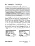
Before any model input can be created, you must plan a system schematic. The schematic is composed of the generalized
building-blocks of the system: nodes and arcs. A diagram of the schematic shows how the nodes and arcs fit together to form
the system. Figure 2.1.0 is an example schematic diagram.
The schematic clearly shows what is in the system, and by implication, what is not. As the modeler, you must decide what
needs to be included in the system and what should be excluded. You cannot model everything, and you should generally
only try to model what you need to. W ithin the system, water is neither created or destroyed. However, it can enter and leave
Figure 2.1.0
Example Schematic
-16-
the system.
W ith OASIS, the schematic is always user-defined and modular. You build the schematic out of nodes and arcs. You may
add new nodes or arcs, remove any nodes or arcs, or modify the descriptive information associated with a node or arc. All
this information is recorded in OASIS's input files. The OASIS GUI contains controls that make if easy to build and modify
the schematic graphically (section 3.7.1)
In the sections that follow, we will discuss the following components of the schematic:
Nodes — points of interest in the system.
Arcs — which convey water from one node to another.
Inflows — the water that enters a node from outside the system (or leaves a node to go outside the system), not
subject to the LP router’s control.
Terminal nodes — at which water can leave the system, subject to the LP router’s control.
2.1.1 NODES
A node represents a point of interest in the system. The complement of the node is the arc. Arcs represent conveyance from
one node to another. In OASIS, every node must have at least one arc connecting to it.
Nodes are basic building blocks of an OASIS model. You specify how many nodes there are, and the descriptive information
about each, by editing OASIS input.
To add a new node to the system, add a record for the node to the Node table (section 4.5.3 part B). There will have to be
at least one arc connecting to this node in the Arc table (section 4.5.3 part C). Depending upon the node type, you may need
to add information to other database tables and OCL.
To remove a node from the system, delete the record for the node from the Node table in the system database (section
4.5.3 part B). Any reference to this node needs to be deleted from all other OASIS input.
Any node can have inflow. If it has positive value, inflow is water entering the node from outside the system. If it has
negative value, it is water leaving the system from the node, and it may be referred to as outflow. See section 2.1.3 and
section 2.4.0 part E for more about inflow.
Every node is identified by a unique node number, and every node has one of three node types: junction, demand, or
reservoir. The node type of every node is given in the Node table.
A. JUNCTION NODES
Junction nodes are the simplest type of nodes. Unlike demand or reservoir nodes, junction nodes are not automatically
associated with any special operating rules. Therefore, there are no special input tables for junction nodes. Junction nodes
are shown in Figure 2.1.0 as circles.
Some of the reasons to use a junction node are:
To model a point in the system where inflow (or outflow) occurs.
To model a point where there is a water-quality boundary condition.
To model a point where conveyance features (represented by arcs) meet.
-17-
B. RESERVOIR NODES
Reservoir nodes are nodes at which water can be stored. OASIS computes the storage at the end of every time step, which is
the storage at the beginning of the next time step. Maintaining storage at a reservoir node is a basic, built-in operating goal.
OASIS has built-in features to model many types of rules associated with a reservoir node, including:
Evaporation (section 2.4.0 part G).
Rule curves or storage targets (section 2.4.0 part H).
Storage-Area-Elevation relationships (section 2.4.0 part F).
Input needed for a reservoir node: For every reservoir node in the system, there must be a record in the Reservoir table
(section 4.5.3 part H) and the Initial Conditions table (section 4.5.6). Though not strictly required, you may also need
information in the Reservoir S-A-E table (section 4.5.3 part J), the Evaporation table (section 4.5.3 part K), and the Weight:
Storage table (section 4.5.7 part B). Note that the Reservoir table and Evaporation table may refer to additional static, timeseries, or OCL input.
Reservoir nodes are shown in Figure 2.1.0 as triangles.
Reservoir nodes would be used to model any storage point in the system, including natural or man-made lakes or ponds,
groundwater basins, or tanks.
C. DEMAND NODES
Demand nodes are nodes to which water is delivered. Delivery to a demand node is a basic, built-in operating goal (section
2.4.0 part D). The delivery may meet, but never exceed, a specified target value referred to simply as the demand. The
deficit between delivery and demand is called shortage.
It is assumed that water delivered to a demand node leaves the system. Consistent with this assumption, it is assumed that
there are no arcs leaving a demand node. However, you are permitted to create arcs that leave a demand node. The water
that flows through these arcs back into the system is called return flow, and it does not have to be equal to the delivery. See
section 2.5.2 for more information about return flow.
Input needed for a demand node: For every demand node in the system, there must be a record in the Demand table
(section 4.5.4 part A). Though it is not strictly required, you should also enter a record in the Weight: Demand table (section
4.5.7 part C). Note that the Demand table may refer to additional static, time-series, or OCL input.
Demand nodes are shown in Figure 2.1.0 as rectangles.
2.1.2 ARCS
An arc represents a conveyance feature in the system. The complement of the arc is the node. Nodes represent points where
conveyance features may join. In OASIS, every arc starts at one node (the upstream node) and ends at another node (the
downstream node). Any node may have more than one arc entering and more than one arc leaving.
Arcs are basic building blocks of an OASIS model. You specify how many arcs there are, and the descriptive information
about each, by editing OASIS input.
To add a new arc to the system, add a record for the arc to the Arc table (section 4.5.3 part C). The arc is identified by its
upstream and downstream nodes. There must be records for both nodes in the Node table (section 4.5.3 part B).
-18-
To remove an arc from the system, delete the record for the arc from the Arc table in the system database (section 4.5.3
part C). Any reference to this arc needs to be deleted from all other OASIS input.
The LP router decides the flow in an arc. Encouraging flow in an arc is a basic, built-in operating goal. Every arc is
directional. That is, the flow is positive when water goes from the upstream to the downstream node. The flow is negative
when it goes from the downstream to the upstream node. This is called reverse flow. The default assumption for an arc is
that there can be no reverse flow -- flow cannot be less than zero. However; you may enable reverse flow by specifying a
maximum reverse flow for the arc. See section 2.4.0 part C for more information.
For each arc, you have the options of specifying three operating criteria:
minimum (target) flow (section 2.4.0 part B): a value of flow which the LP router tries to meet. There is no default
minimum (target) flow in an arc— you must specify if there is one.
maximum flow (section 2.4.0 part A): an upper bound on the flow in the arc. The default is that there is no
maximum flow in an arc— you must specify if there is one.
maximum reverse flow (section 2.4.0 part C): a lower bound on the flow in the arc. The default is that the lower
bound on flow is zero— you must specify if the lower bound is anything different.
Arcs are represented in Figure 2.1.0 by arrows that connect nodes.
2.1.3 INFLOW
Inflow is water entering the system at a node, not subject to control by the LP router. If the value of the inflow is negative,
then the water is actually leaving the system from a node, not subject to control by the LP router. This negative inflow could
be called outflow, but in OASIS the term inflow is used to mean both positive and negative inflows. At any node, the inflow
could be positive at some time steps and negative at others.
There can be no more than one inflow value given for each node.
The inflow is not controlled by the LP router, but is computed before the routing problem is solved. The value of inflow is
thus incorporated into the continuity-of-flow constraint (section 2.2.4) at any node that has inflow. See section 2.2.0 for
discussion of the LP router. The inflow values can be given in a database, or computed in OCL.
To apply inflow at a node: Edit the Inflow field for the node in the Node table (section 4.5.3 part B). The entry in this field
tells OASIS how to find the inflow values. Depending upon the entry, you need to enter supporting information in a pattern
table, a time-series table, or in OCL. If the Inflow field is blank, there will be no inflow at the node.
Inflows are shown in Figure 2.1.0 by arrows that end at nodes but do not originate at other nodes.
2.1.4 TERMINAL NODES
A terminal node is a node where the router can send water out of the system. That is, all water that enters a terminal node is
leaving the system. This is to be distinguished from the inflow discussed in section 2.1.3, because the LP router decides how
much water leaves the system at a terminal node. Of course, the router’s decision is determined by the operating rules that
you give to it. See section 2.2.0 for more on the LP router.
A terminal node is not a node type like junction, reservoir, and demand. Either junction nodes or reservoir nodes may be
terminal nodes. Demand nodes are not referred to as terminal nodes, although a demand node without return flow does
behave similarly to a terminal node.
-19-
A terminal node is any junction or reservoir node that has
no arcs leaving it.
no arcs entering that can have reverse flow.
To create a terminal node, add a record for the node to the Node table (section 4.5.3 part B). There has to be at least one
arc entering this node listed in the Arc table (section 4.5.3 part C), but no arcs leaving the node. None of the arcs that enter
this node may be capable of reverse flow.
OASIS does not write a continuity-of-flow constraint (section 2.2.4) to the LP for terminal nodes, and it does not display a
balance sheet for a terminal node in the balance-sheet output (section 5.2.0).
It is good practice to have only one terminal node in a system, so that it is easily recognized as the terminal node. However,
you may create as many terminal nodes as you like.
2.2.0 DECIDING HOW WATER IS ROUTED
OASIS is designed so that the decisions in a water system are simulated by a linear-programming (LP) router. The design
of OASIS is intended so that you do not need previous experience with LP in order to use OASIS, and this documentation
strives to minimize reliance on LP terminology. Chapter 7 provides a more technical reference for those who need better
understanding of the LP.
W ithin this LP router is the mixed-integer LP-solving package called XA, developed by Sunset Software Technology. The LP
router consists of XA, plus those routines in OASIS that write out the LP problem set, feed it to XA to solve, and receive the
results from XA. The results that XA gives to OASIS comprise a simultaneous solution of all the decision variables (the
unknowns).
The LP problem set (or just the LP) is a set of mathematical statements that are linear with respect to the unknowns, or
decision variables. Non-decision variables go into the LP as values, so the rules do not have to be linear with respect to any
non-decision variables.
W e have divided the operating rules that the LP expresses into two categories: goals and constraints. Every rule is either a
goal or a constraint, as we will explain in the following sections.
2.2.1 DECISION VARIABLES
Decision variables are the unknown variables whose values the LP router solves, or “decides”. The principal decision
variables are:
Flow in an arc. For every arc you enter into OASIS, the LP router automatically creates a flow variable.
Storage at a reservoir node. For every reservoir node you enter into OASIS, the LP router automatically creates a
storage variable.
Delivery at a demand node. For every demand node you enter into OASIS, the LP router automatically creates a
delivery variable.
There are other decision variables which are documented in section 7.2.0, although you should not need to know about them
until you have some experience with OASIS. You may create new decision variables with the OCL udef command (section
2.5.1 part A).
-20-
2.2.2 OPERATING CONSTRAINTS
Operating constraints are rules that the LP router can not violate. They may be expressed as equalities, such as:
QT100101 + QT400101 = QT101333 + 456.7
Or they may be inequalities, such as:
QT101333 < QT500600 - 300.33
In these examples, the QT variables are actual names for flow variables that could be written to the OASIS LP. Although
most users should not need to refer to the LP in this form, there is a complete description of the QT variables and other parts
of the LP in Chapter 7.
W hen the LP router solves, it must comply with all of the constraints in the LP. If a solution cannot be found that satisfies all
of the constraints, then the LP is infeasible. An infeasible LP causes a fatal error in an OASIS run.
Constraints are often used to define physical rules in the system, or to define the relationships between variables. A constraint
would not be used to model such rules as “deliver water to node 300", “maintain in-stream flow in arc 120.670", or “keep at
least 400 million gallons of water in reservoir node 346". These are rules which can not be met under all circumstances, so
they should be modeled as goals.
OASIS models many of the standard operations as constraints or parts of constraints that it automatically adds to the LP. For
example, the model never loses or “creates” water in its accounting because every node has a continuity-of-flow constraint
(section 2.2.4). Inflow and evaporation are two of the terms in the continuity-of-flow constraint. You may define a standard
maximum flow for an arc, which constrains that flow from being more than an upper limit. Another standard constraint is the
fact that the delivery to a demand node can never be more than the demand. You can create new constraints of your own
design with OCL commands (section 2.5.0).
W hen developing a new rule, you must determine whether to enter it into OASIS as a goal or a constraint. If the rule is not a
relationship that absolutely must be obeyed, then it probably should be a goal, not a constraint.
2.2.3 OPERATING GOALS AND WEIGHTS
Operating goals are rules that express routing decisions the LP router should try to make. Meeting a goal is not a matter of
violating or not violating a rule. Furthermore, we don’t think of the router as being “forced” to meet a goal. Some examples
of goals are:
Deliver as much as possible to demand node 340
Route as much flow as possible through arc 901.234
Do not route any flow through arc 901.234 unless absolutely necessary.
Prefer to route flow through arc 320.100 before routing any through arc 600.200, but prefer routing flow through arc
600.200 over arc 789.123.
Operating goals are a very powerful tool in OASIS, and you must appreciate this in order to use OASIS effectively. Note that
all of the above examples express operations that might not always be possible to satisfy. If we wanted to express these rules
as constraints, we would have to write lots of conditions to compute things like “how much is possible”, “is absolutely
necessary”, “the first one is full, so we can put some into the second one”, and “the second one is not full, so none goes into
the third one”. But with OASIS we simply and easily express what the goals are, and we let the LP router determine how to
meet the goals.
The last of the above examples illustrates the important fact that goals are by their very nature in competition with other
goals. It is expected that sometimes some goals will have to be met at the expense of others. Therefore, we rank the goals by
giving each one a weight or penalty. A penalty is simply another word for a negative weight.
-21-
One place you provide weight values is in the weights database file (section 4.5.7). The weights given in this file are assigned
to standard decision variables, such as storage, flow, and delivery. As the LP router solves, we can think of it as scoring
points for each decision variable. The score is equal to the weight value times the value of the decision variable. For
example, if the weight on the flow through an arc is 50 points, and the value of the flow is three volume units, then the router
receives 150 points. The router will solve the LP routing problem so that it receives the maximum possible points. This is
what LP solvers do, and you do not need to know how it does it.
To help understand weights, consider the following facts:
Positive weight on a decision variable encourages the LP router to maximize the value of that variable as much as it
can.
Negative weight on a decision variable encourages the LP router to minimize the value of that variable as much as it
can.
The LP router is indifferent to the value of a variable whose weight is zero.
The router does what it can to move water from lower weight to higher weight.
W hen there is more than one possible routing decision, the router makes the decision that gets the highest net number
of points.
W hen there is more than one possible routing decision that get the same number of net points, the router is
indifferent as to which one is chosen. This results in alternate optima. See section 2.2.5 for more discussion of
alternate optima.
Remember that what is possible for the router is defined by the set of constraints. See section 2.2.2 for a discussion of
constraints.
Besides the weights database file, you can apply weights through OCL. W ith the target command (section 2.5.1 part E), you
apply a penalty to the deviation of a user-defined target value from a user-defined target expression. W ith the minimax
command (section 2.5.1 part F), you apply a penalty to a minimax variable, which will tend to equalize two or more userdefined quantities.
In summary, you can define the following goals for OASIS:
W eight entered in the weights database file (section 4.5.7) encourages the router to maximize or minimize standard
decision variables: flow, storage, and delivery. For example, weight on a storage variable defines a goal of keeping
or increasing water in storage.
The OCL target command (section 2.5.1 part E) defines a goal of making a user-defined target value equal to a userdefined target expression.
The OCL minimax command (section 2.5.1 part F) defines a goal of equalizing two or more user-defined quantities.
It does this by minimizing the largest of those quantities.
All of these goals are defined by their weights. If you forget to apply a weight, or make it zero, it is as if the goal did not
exist.
-22-
2.2.4 CONTINUITY-OF-FLOW CONSTRAINTS
There is one especially important constraint that we must discuss now. This is the continuity-of-flow constraint, which
OASIS automatically generates for every node in the system (except terminal nodes) and enters into the LP. Once you
understand that the continuity-of-flow constraints are being automatically generated, you can usually take them for granted.
However, it is useful to understand some things about them.
The continuity-of-flow constraints ensure that the model obeys the physical truth that mass (or volume) is conserved as water
flows. At a junction node, the continuity-of-flow constraint has this form:
(sum of arc-flow in) + (inflow) = (sum of arc-flow out)
The arc-flow in and the arc-flow out are decision variables, but the inflow is a known quantity. This constraint assures that if
a volume of water goes into a node, the same volume of water comes out — it can not leave the system, unless you
specifically create a negative inflow value at the node.
At a reservoir node, the continuity-of-flow constraint has this form:
(sum of arc-flow in) + (inflow) - (evaporation)
+ (beginning-of-period storage)
= (sum of arc-flow out) + (end-of-period storage)
The arc-flow in, the arc-flow out, and the end-of-period storage are decision variables, but the inflow, evaporation, and
beginning-of-period storage are known quantities.
At a demand node, the continuity-of-flow constraint has this form:
(sum of arc-flow in) + (inflow) = (delivery)
The arc-flow in and the delivery are decision variables, but the inflow is a known quantity. Note that arc-flow out is not part
of this constraint. It is assumed that you will not create arcs that come out of a demand node. However, if you do, they will
still not be written into the continuity-of-flow constraint. See section 2.5.2 for more on how to handle this.
At a terminal node, no continuity-of-flow constraint is written. Thus, water that goes into a terminal node does not stay in
the system.
Notice that the evaporation and inflow terms are part of the continuity-of-flow constraints, and they are known quantities.
Thus, we can say that the system is constrained to these exchanges with the outside world, and the router can not change the
value of the exchanges. Therefore, if the inflow or evaporation can not be accommodated in the system (that is, in conflict
with other constraints), then you could have an infeasible LP, and OASIS would experience a fatal error.
-23-
2.2.5 ALTERNATE OPTIMA
W e said in section 2.2.3 that the LP router always finds the maximum number of points that can be earned from the weight
values. However, there may be more than one way to earn that maximum number of points. If so, then we say there are
alternate optima. Consider this simple example of a system with only three nodes:
Initial volume stored in each reservoir node: 100 AF
Demand at node 906: 20 AF
Maximum flow through arc 500.906: 8 AF/period
Maximum flow through arc 555.906: 16 AF/period
W eight on storage in each reservoir node: 2
W eight on delivery to node 906: 10
No inflow or evaporation.
Figure 2.2.5
Example of Alternate Optima
The maximum number of points that the LP router can earn is 200 points for a full delivery to node 906 plus 360 points for
leaving the rest of the water in storage in the two reservoir nodes (560 points total). This could be accomplished by taking 8
AF from node 500 and 12 AF from node 555. It could also be done by taking 4 AF from node 500 and 16 AF from node 555,
and there are a infinite possibilities between these two options! These are the alternate optima.
W hich of the infinite ways will the LP router choose? In fact, there is no way to predict what the LP router will do here. By
making the weights equal on the two reservoirs, you are effectively telling the LP router that it doesn’t matter!
Usually, you should try to avoid alternate optima, because it may lead to inconsistent results. However, when using multiple
priority levels, you will actually want alternate optima in the early priority levels, so that the LP router can choose from
among the alternate optima in later priority levels. That is, you will want to create alternate optima on purpose. See section
2.2.6 for more about priority levels.
In the above example, we could avoid alternate optima by giving different weights to the two reservoir nodes. Suppose the
water from reservoir 555 is more desirable. W e could change the weight on reservoir node 500 to 3, and the weight on
reservoir node 555 remains at 2. Now there is only one way for the LP router to maximize the points earned. It will take 16
AF from node 555, and 4 AF from node 500, to earn a total of 656 points.
W hat if we want to model a rule that specifies equal use of the two reservoirs? This rule could be a goal to try to make the
flow out of the reservoirs equal, or to try to make the storage in the two reservoirs equal. Either way, we could model the
situation by using the equal storage weights from the original example, and adding a m inim ax command. The minimax
command allows you to model a goal of keeping two or more quantities equal. Furthermore, the addition of a minimax
command would mean that there are no longer alternate optima. See section 2.5.1 part F for more about minimaxes. Please
note that without the minimax command, there is nothing in the original example that tells OASIS to try to balance its use of
the two reservoirs.
-24-
2.2.6 PRIORITY LEVELS
Multiple priority levels are an advanced feature that are usually not needed for models of small systems. However, they are a
powerful tool in OASIS, and they make it possible to model some very complex operational rules.
In OASIS, every weight value is associated with a priority level 1-6. You specify what the priority level is when you enter the
weight or penalty input. Therefore, it can be said that every operating goal is associated with a particular priority level.
OASIS calls the LP solver at least once for each priority level. In general, priority 1 is the first call to the solver, priority 2 is
the second, and so on.
OASIS determines how many priority levels there are by the largest priority number that you enter in the input. For example,
if the highest priority number that you have assigned to any weights is 3, then there are three priority levels.
The process of solving each priority level involves these steps:
1.
OASIS solves the LP, using only the weights of the current priority level.
2.
OASIS adds a constraint which restricts the decisions to the alternate optima (section 2.2.5) of the priority level
that was just solved.
3.
For each additional priority level, OASIS returns to step 1.
If there is only one priority level, then this process is trivial, and you do not need to worry about how the LP router handles
multiple priority levels.
To make sure there is only one priority level, make sure that all of the priority level entries in the weights database (section
4.5.7) are “1", and all of the priority fields in the OCL target (section 2.5.1 part E) and minimax (section 2.5.1 part F)
commands have “1" in them.
Notice that step 2 constrains the solution of the next priority level to the alternate optima of the priority level that was just
solved. In order to use priority levels effectively, you must design your weights so that there are alternate optima within the
earlier priority levels. If well designed, your set of weights and priorities “close in” on a single, correct solution by reducing
the alternate optima. Thus, you would not want alternate optima in the last priority level. See section 2.2.5 for discussion of
alternate optima.
Since many models do not need them, why would you ever want to use multiple priority levels? There are two very good
reasons.
Avoid excessive scaling of weights. If you have a very complicated system, with a very large number of competing
operating goals, you could develop a large range of weights. For example, some of your weight values might be
20000, 3000, 500, 100, 20, 5, and 1. It can be confusing to keep track of these different scales. Furthermore, it may
strain the computational precision of the LP solver. Therefore, a complicated system may be easier to model with
multiple priority levels.
W eights in one priority level do not have additive effects with weights in another priority level. W ithin a
priority level, each potential routing decision must be considered by the net number of points that the router would
earn from that decision. W hen there are a large number of operating goals involved in a decision, you have to add
together the points contributed by each goal in order to understand where the water will go. Sometimes you want the
weights to add together, sometimes you do not. If you want the weights to add together, put them in the same
priority level. If you do not want them to add together, you may be able to put them into different priority levels.
This can reduce a great deal of confusion.
-25-
A third use of multiple priority levels relies on an alteration of the definition of a priority level.
Use the LP router to compute “what-if” information. That is, you need information about how the system would
operate if there were a different set of goals than those that ultimately determine the routing decision. This is a very
advanced use of OASIS. In order to do this, you must use the OCL cancel command (section 2.5.1 part H). If a
priority level has been canceled, then subsequent priority levels are not constrained to the alternate optima of that
priority level.
Multiple priority levels cannot be combined with multiple-period-optimization (MPO) (section 2.2.7).
2.2.7 MULTIPLE-PERIOD OPTIMIZATION (MPO)
OASIS supports multiple-period optimization (M PO), meaning that the LP router is able to compute decisions for more
than one time step in a single solve. You may also use MPO to have OASIS do no LP solve during particular time steps.
Solving for one time step at a time is considered the standard mode of operation for OASIS, and we consider MPO to be a
very advanced feature which most users do not need. W e recommend you skip reading this section unless you plan to use
MPO.
To understand the discussion of MPO steps, you probably need to understand how OASIS simulates a time cycle (section
2.8.1).
In order to do MPO, you must be using the Steps input table (section 4.5.2 part D). For each step of the time cycle, you
assign a number of time steps to solve through the Solve field of the Steps table. An entry of zero means do not do any LP
solve. An entry of 1 means solve an LP for the current step (as in the standard case). An entry of 2 means that a single LP
solve is done for the current step and the first step after it. In the latter case, we say there are two M PO steps. An entry of 3
means that a single LP solve is done for the current step and the next two steps after it. In this case, we say there are three
MPO steps. OASIS does not have a strict upper limit on the number of MPO steps.
Note that MPO cannot be combined with multiple priority levels (section 2.2.6). If you use multiple priority levels, all time
steps in the Steps table must have an entry of 1 in the Solve field. If you are doing MPO, then all weights must have a priority
level of 1.
To do MPO, edit the Solve field of the Steps table (section 4.5.2 part D). Entries greater than 1 indicate that more than one
time step is solved during the given time step. Make sure that there is only one priority level (section 2.2.6).
To make sure that you are not doing MPO, make sure that all entries in the Solve field of the Steps table (section 4.5.2 part
D) are “1". If you are not using a Steps table, then you can be sure you are not doing MPO.
There are different ways to use MPO. One is to simulate a decision-making process where decisions that span several steps
are made at one time, and are not changed. For example, suppose our time cycle is one week, and our time step is one day.
Thus, there are seven steps in the cycle. Using the Solve field of the Steps table, we can assign seven M PO steps to the first
-26-
day of the week, and zero to the rest. Refer to the table below, which contains some of the information from the Steps table.
This would mean that all routing for the entire week is decided at the start of the week, and it is not changed as the week goes
on. The decisions for days two through seven were solved on day one. When OASIS evaluates days two through seven, it
does not change any decision variables, because the number of MPO steps assigned to those days is zero.
Step Number
Number of MPO steps (Solve field)
1
7
2
0
3
0
4
0
5
0
6
0
7
0
Another way to use MPO is to simulate a process where current decisions account for future decisions, but the decisions can
always be updated using current information. For example, suppose our time step is one day. Our time cycle only contains
one step, and we assign that step with three MPO steps. Refer to the table below, which contains some of the information
from the Steps table. Thus, every time step of the simulation, OASIS will make decisions for the current step plus the next
two future steps. The information for decisions of these future steps remains in memory until the next solve. W hen these
steps become the current step, that information can be put to use, but the new solve of the current step overwrites the values
that were given during the previous step. This differs from the previous example, where no overwriting was done.
Step Number
1
Number of MPO steps (Solve field)
3
W hen doing MPO, you should be mindful of the assumptions about future knowledge, and whether they are appropriate to
your analysis. You do have alternatives to assuming perfect future knowledge. W hen evaluating a time step that uses MPO
you can use the OCL Set command (section 2.5.1 part C) to set the future value of a variable such as inflow. This future value
could be computed using the assumptions and available information of a real-world forecast. In subsequent steps, you can
overwrite these future values as the information improves.
W hen OASIS creates the LP for a time step that contains MPO:
There is a separate instance of each decision variable (section 7.2.0) for each MPO step. For example, if there is a
reservoir with node number 100, and there are two MPO steps, then the LP contains one variable for storage in
reservoir 100 at the end of the current step, and another variable for storage in reservoir 100 in the following step.
See section 7.4.0 for more on the multiple copies of each variable.
For weights entered in the weights database (section 4.5.7), each instance of a given variable receives the same
weight. This rule is applied differently to weights on reservoir storage – see section 4.5.7 part B.
There is a separate instance of each LP constraint (section 7.3.0) for each MPO step. See section 7.4.0 for more
details.
All OCL commands (section 2.5.1) that precede the command solve (section 2.5.1 part G) are evaluated once for
each MPO step. First, OASIS evaluates all OCL commands for the first MPO step. W hen the solve command is
encountered, it repeats the entire list of OCL commands for the second MPO step, and so forth. During this
iteration, the value of the OCL variable MPO_step (section 4.7.4) changes to reflect the MPO step currently under
evaluation. W hen this process has been finished for all MPO steps, the LP is solved. Those OCL commands that
follow the solve command are not evaluated multiple times for M PO steps.
As mentioned above, there is an instance of each decision variable for each MPO step. In OCL, you distinguish
between the different instances of decision variables by using time indices (section 4.7.4 part A). If you are not
doing MPO, then the time indices cannot be applied to decision variables.
-27-
In OCL, you can apply the flag NoMultiple to the Udef (section 4.7.2 part B), Target (section 4.7.2 part E), and
Constraint (section 4.7.2 part D) commands. This flag tells OASIS to evaluate the particular command or variable
only once per time step. In other words, it suppresses the default rule to evaluate a separate instance of the command
or variable for each MPO step. W hen NoMultiple is used, the evaluation is done during the first MPO step of the
time step.
Some of OASIS’ standard computations are more difficult with MPO. Reservoir elevation (section 2.4.0 part F),
area, and evaporation (section 2.4.0 part G) are always computed after the LP has been solved. However, when
evaluating for MPO, this means that these values cannot be evaluated until all of the steps have been solved. Thus,
OASIS assumes that these variables are equal to their values at the beginning of the first MPO step.
-28-
2.3.0 MODEL INPUT
W ith OASIS, your model is completely user-defined. You define the model by entering its description in input files. Every
time OASIS is run, it reads the information from the input files. The input includes files in different formats, including MS
Access, ASCII (plain text), and HEC-DSS.
The input files are managed by the OASIS GUI. The GUI provides controls for editing the input that is stored in text files
and MS Access files. For OCL files, the GUI passes control to a program called VEDIT. For HEC-DSS files, the GUI passes
control to a program called HecDssVue. See Chapter 3 for complete documentation of the GUI.
For users who are comfortable with managing computer files and working with OASIS, the input files can be edited with
third-party software – working outside the GUI. For example, MS Access files can be edited with MS Access. ASCII files
can be edited with a text editor, such as VEDIT, W indows W ordPad, or a word processor program. HEC-DSS files must be
edited with DSS utility programs.
There are certain input parameters that can be specified in the command line. See section 4.1.0 for more information.
2.3.1 RUN DIRECTORY
OASIS input is organized so that all input files belonging to a particular simulation run can be found in a single directory,
called the run directory. All output files are written to this directory as well. This way, all the files that belong to a particular
simulation run are contained in one place, distinct from the files of any other run.
You tell OASIS what the run directory is by entering its name in the model pointer file, which is always named directry.nam
(section 4.3.0). Alternatively, you can specify the name of the run directory with the command-line parameter DIR (section
4.1.0).
W hen you provide the names of input files, you can give them with relative or absolute path information. Thus, you can
easily organize your files into subdirectories of the run directory. These paths can also use the “directory up” symbol, a pair
of dots, to locate files outside of the run directory. An absolute path can also be used to locate files outside of the run
directory. For example, you might wish for several different runs to rely on a single copy of a certain input file. This way, a
change to that one input file will automatically be changed for all of those runs. It would be logical to place this file outside
of the individual run directories.
The OASIS GUI has many features that make it easy to manage run directories (section 3.4.0). However, the GUI also
imposes more rigid requirements on the format of the run directory. Consult with HydroLogics staff if you wish to locate
certain files outside the run directory but aren't sure whether it will work with the GUI.
-29-
2.3.2 FILES THAT OASIS READS
The simulation program model.exe reads several different input files, which are listed below. Chapter 3 tells how these files
are organized for use with the GUI. Chapter 3 also lists other files that are not necessarily read by model.exe, but by other
programs in the OASIS package.
Note that the static databases (items D through I and item L below) can be combined together. For example, the seven static
databases can be combined into one large database. See 4.5.0 for more information.
A.
Identity Key. OASIS reads this file to get information about the user license, which it prints in its run window and
in output files. See section 4.2.0 for reference.
B.
Pointer File. This ASCII file is always named directry.nam and is located in the same directory as the OASIS
executable file. OASIS reads this file to learn the name of the run directory. See section 4.3.0 for reference.
C.
Control file. This ASCII file is found in the run directory. OASIS reads this file to learn the names and paths of the
various input files, the name and path of the output file, and some output flags. See section 4.4.0 for reference.
D.
Time parameters database. The name and path of this MS Access file is given in the control file. OASIS reads
this file to learn the size of the time step, the first and last time steps to simulate, whether to work in water years or
regular years, and other parameters related to the computation of time. See section 4.5.2 for reference.
E.
System database. The name and path of this MS Access file is given in the control file. OASIS reads this file to
learn the units-of-measurement system, nodes and arcs in the system, as well as parameters describing the arcs,
reservoir nodes, and water quality. It may read formatting information for the balance sheet output. See section
4.5.3 for reference.
F.
Demand database. The name and path of this MS Access file is given in the control file. OASIS reads this file to
learn parameters describing the demand nodes. See section 4.5.4 for reference.
G.
Inflow database. The name and path of this MS Access file is given in the control file. OASIS reads this file to
learn parameters describing the inflows and water quality. See section 4.5.5 for reference.
H.
Initial conditions database. The name and path of this MS Access file is given in the control file. OASIS reads
this file to learn the storage and water quality values in reservoirs at the beginning of the first time step of simulation.
See section 4.5.6 for reference.
I.
W eights database. The name and path of this MS Access file is given in the control file. OASIS reads this file to
learn the weights to apply to the standard decision variables. See section 4.5.7 for reference.
J.
OCL file. The name and path of this ASCII file is given in the control file. OASIS reads this file to get special
operating rules that you define with OCL commands. See section 4.7.0 for more information.
K.
OCL static database. The name and path of this MS Access file is given in the OCL file. This file is optional.
From this file, OASIS gets supplemental data referred to in the OCL file, including pattern data and look-up tables.
See section 4.5.8 for reference.
L.
Time-series files. The names and paths of these files are given in the OCL file and in the File ID tables of some of
the MS Access databases. These files are optional. From these files, OASIS gets supplemental data referred to in
the OCL file or in the static databases. See section 4.6.0 for reference.
-30-
2.4.0 STANDARD OPERATING RULES
You tell OASIS what are the operating rules of the system by editing OASIS’s input files. There are two conceptual tiers to
OASIS input: standard input, and OCL input. Standard input allows you to create rules of a standardized form. This is
often useful, because most water resources systems have similar types of rules. W ith these standardized forms, you merely
supply parameter values that define the rule.
OCL input allows you to create rules with forms of your own design. This makes OASIS much more flexible. Section 2.5.0
discusses OCL operating rules.
The present section discusses each of the standard operating rules. It tells you how to handle the input for the common uses
of each operating rule. Each of the standard operating rules was developed to model a certain common situation in a water
resources system. However, in the description of each operating rule, we note that you are free to find creative uses for the
standard rules. There are also alternative ways to model almost any problem.
A. MAXIMUM FLOW IN AN ARC
By default, there is no maximum flow in an arc. You may apply a standard maximum-flow constraint to any arc. Because
this maximum flow is a constraint, it can cause an infeasible LP if it conflicts with other constraints.
You tell OASIS whether there is a maximum-flow constraint on each arc in the Arc table. The code in the Arc table tells
where the values of the maximum flow are found. You can specify the values with pattern, time-series, or OCL input. See
section 4.5.3 part C for complete information.
To add, change, view, or remove a maximum-flow constraint at an arc, open the Arc table (section 4.5.3 part C). Find
the record for the arc, and the Max Flow field. The code in this field tells whether the maximum-flow values are stored in a
pattern table, a time series table, or in the OCL file. Go to the appropriate one of these three data sources to view or change
the data. If this field is blank, then there is no maximum flow at the arc. Furthermore, you can change the source of the data
from one type to another (for example, from pattern to OCL). See section 4.5.3 part C for complete information.
The maximum flow is generally used to model the physical capacity of a conveyance feature. It can also be used to model a
maximum that is dictated by policy. You are free to find creative uses for the standard maximum flow — only remember that
it is a constraint. Many policy maximum rules, such as flood control levels, can be violated under extreme circumstances, so
they should not be modeled as constraints.
There are many alternatives to the standard input for maximum flow in an arc. You can use the standard minimum (target)
flow to create a maximum flow target (goal) (section 2.4.0 part B). You can also use the OCL constraint command to create
a maximum flow constraint (section 2.5.1 part D). The OCL target command (section 2.5.1 part E) could be used to create a
maximum flow constraint or target.
B. MINIMUM (TARGET) FLOW IN AN ARC
The standard minimum-flow rule in OASIS could more appropriately be called a target flow. One reason is that it defines an
operating goal, not a minimum-flow constraint. The other reason is that it could actually be used to model a maximum flow.
However, the name minimum flow has long been applied to this standard rule, so the name stays for continuity.
By default, there is no minimum (target) flow at an arc. You may apply a minimum-flow goal to any arc. Because this
minimum flow is a goal, it cannot be the direct cause of an infeasible LP.
You tell OASIS whether there is a minimum (target) flow on each arc in the Arc table. The code in the Arc table tells where
the values of the minimum (target) flow are found. You can specify the values with pattern, time-series, or OCL input. See
section 4.5.3 part C for complete information.
-31-
To add, change, view, or remove a minimum (target) flow at an arc, open the Arc table (section 4.5.3 part C). Find the
record for the arc, and the Min Flow field. The code in this field tells whether the minimum-flow values are stored in a pattern
table, a time series table, or in the OCL file. Go to the appropriate one of these three data sources to view or change the
data. If this field is blank, then there is no minimum flow at the arc. Furthermore, you can change the source of the data from
one type to another (for example, from pattern to OCL). See section 4.5.3 part C for complete information.
Because this is an operating goal, there must be weight associated with it. Thus, there must be a record in the Weight: Arc
table (section 4.5.7 part A) for any arc that has a standard minimum-flow rule. The weight value in the A Wt field enforces the
minimum flow. There must be an accompanying priority level in the A Pri field. Make sure that the weight in the A Wt field is
higher than the weight in the B Wt field.
The minimum (target) flow is commonly used to model in-stream flow rules, such as the rules we often find below a dam to
maintain habitat or water quality. It can be used to model any kind of policy flow target. You are free to find creative uses
for the standard minimum flow — only remember that the LP router is never constrained to meet the minimum flow.
There are many alternatives to the standard input for minimum (target) flow in an arc. You can use the standard maximumreverse-flow rule to create a minimum-flow constraint (section 2.4.0 part C). You can also use the OCL constraint command
to create a minimum-flow constraint (section 2.5.1 part D). The OCL target command could be used to create a minimumflow constraint or target (section 2.5.1 part E).
The standard minimum (target) flow rule can actually be used to model a maximum-flow target. The only trick to doing so is
that the weight on exceeding the minimum-flow value would have to be negative.
To make a maximum-flow target at an arc, follow all the steps for creating a standard minimum-flow target, knowing that
the values labeled as a minimum flow are really maximum-flow values. In the Weight: Arc table (section 4.5.7 part A) make
the value in the B Wt field negative. There must be an accompanying priority level in the B Pri field. Make sure that the
weight in the A Wt field is higher than the weight in the B Wt field.
C. MAXIMUM REVERSE FLOW IN AN ARC
The standard rule for maximum reverse flow is really a minimum-flow constraint. However, the name minimum flow is
already used by the standard rule for minimum (target) flow. Furthermore, the name maximum reverse flow is quite
appropriate for the most common use of this standard rule.
By default, the flow in an arc is constrained to be no less than zero, making the arc unidirectional. You may apply a standard
maximum reverse flow constraint to any arc. If an arc has a negative value for the maximum reverse flow, then it is a twoway arc, capable of reverse flow. Because the maximum reverse flow is a constraint, it can cause an infeasible LP if it
conflicts with other constraints.
You tell OASIS whether there is a maximum-reverse-flow constraint on each arc in the Arc table. The code in the Arc table
tells where the values of the maximum reverse flow are found. You can specify the values with pattern, time-series, or OCL
input; or as a mirror of the maximum flow. See section 4.5.3 part C for complete information.
To add, change, view, or remove a maximum-reverse-flow constraint at an arc, open the Arc table (section 4.5.3 part C).
Find the record for the arc, and the MaxRev Flow field. The code in this field tells whether the maximum-reverse-flow values
are stored in a pattern table, a time series table, or in the OCL file. Go to the appropriate one of these three data sources to
view or change the data. If this field is blank, then the flow in the arc can be no less than zero. Furthermore, you can change
the source of the data from one type to another (for example, from pattern to OCL). See section 4.5.3 part C for complete
information.
-32-
To make the maximum reverse flow in an arc equal (but opposite) to the maximum flow, open the Arc table (section
4.5.3 part C). Find the record for the arc, and the MaxRev Flow field. Change the code in this field to MIRROR. OASIS will
automatically set the maximum reverse flow to be the negative of the maximum flow, no matter where the maximum-flow
values come from. Do not try to enter values for the maximum reverse flow.
To make an arc with unlimited flow in the reverse direction, open the Arc table (section 4.5.3 part C). Find the record for
the arc, and the MaxRev Flow field. Change the code in this field to MIRROR. Make sure the entry in the Max Flow field is
blank. Do not try to enter values for the maximum reverse flow.
If the maximum reverse flow has a positive value, then you do not have a two-way arc, but rather an arc where the flow is
constrained to be no less than some positive value.
Specifying a maximum reverse flow is the only way to enable two-way flow in an arc. However if you have a two-way arc,
you can always constrain the reverse flow further with the OCL constraint command (section 2.5.1 part D), or set a target or a
constraint with the OCL target command (section 2.5.1 part E).
D. DEMAND AND DELIVERY
Every demand node has a demand value, usually referred to simply as the demand. The water routed into the demand node is
called delivery. The demand minus the delivery is the shortage. It is a standard operating goal to deliver water to a demand
node. As a goal, this rule can not be implicated as a cause of an infeasible LP. There are also standard operating constraints
on the delivery. Specifically, the delivery can not be less than zero or more than the demand. It is possible that these
constraints could contribute to an infeasible LP.
By default, OASIS assumes that water delivered to a demand node leaves the system. If you attach arcs to a demand node to
return water to the system, OASIS does not automatically constrain continuity of flow between these arcs and the demand
node. See section 2.5.2 for an explanation of how to handle return flow.
You tell OASIS where to get the demand values for each demand node through a code in the Demand table (section 4.5.4 part
A). The code tells whether the values are specified with pattern, time-series, or OCL input. See section 4.5.4 part A for
complete information.
To change or view the demand at a demand node, open the Demand table (section 4.5.4 part A). Find the record for the
node, and the Demand Type field. The code in this field tells whether the demand values are stored in a pattern table, a time
series table, or in the OCL file. Go to the appropriate one of these three data sources to view or change the data. You can
change the source of the data from one type to another (for example, from pattern to OCL). See section 4.5.4 part A for
complete information.
Because this is an operating goal, there must be weight associated with it. Thus, there must be a record in the Weight:
Demand table (section 4.5.7 part C) for each demand node. The weight value in the Wt field enforces the demand. There
must be an accompanying priority level in the Pri field.
The standard demand rule can be used to model any feature where water from the system is consumed. It can also be used to
model features where water should be delivered, but some or all returns to the system (if you want to model delivery that
returns to the system, see section 2.5.2). You are free to find creative uses for demand nodes — only remember that the LP
router is never constrained to make deliveries, and it is always constrained from delivering more than the demand.
There are alternatives to using a demand node. If you want to model a demand where all of the delivery leaves the system,
you can create a terminal node (section 2.1.4), and use any combination of the OCL constraint command (section 2.5.1 part
D), OCL target command (section 2.5.1 part E), standard maximum flow (section 2.4.0 part A), standard minimum (target)
flow (section 2.4.0 part B), and arc weights (section 2.2.3) to make rules for the flow into the terminal node. You could also
use such rules at a non-terminal node, or at a combination of terminal nodes and non-terminal nodes.
-33-
E. INFLOW
By default, there is no inflow at a node. You may apply inflow to any node. A node cannot have more than one inflow value.
The value of the inflow is included in the continuity-of-flow constraint (section 2.2.4), so the LP router is constrained to
route the inflow. Therefore, it is possible that the inflow could be the direct cause of an infeasible LP. See section 2.1.3 for
more discussion of inflow.
The standard inflow feature can be used to model any exchange between the system and the outside world, whether the water
is coming into the system (positive inflow) or going out of the system (negative inflow). You are free to find creative uses for
inflow — only remember that the LP router is constrained to send the water into or out of the system, and the value of the
inflow is known before the LP is solved. Thus, the inflow can not be affected by any other LP operating goals or constraints.
There are alternatives to using the standard inflow. Evaporation from a reservoir node (section 2.4.0 part G), also a
constraint, is another exchange between the system and the outside world. If you want to model an exchange with the outside
world that is subject to the LP router’s control, you can make use of terminal nodes (section 2.1.4). At any terminal node, the
LP router can decide how much water is sent out of the system. Bringing water into the system is slightly more complicated,
but it can be done by creating a virtually unlimited source of water. This source would only be a modeling artifact; it is there
so the router can draw water from the source, as needed, and bring the water into the system.
F. RESERVOIR ELEVATION AND SURFACE AREA
The standard rules in the LP are all stated in terms of volume — either the volume of water stored in a reservoir node or the
volume of water that flows through an arc in a period. Reservoir elevation and surface area are not directly part of the LP, but
are computed after the LP has been solved. Both elevation and surface area are functions of the storage at the reservoir node.
You may supply elevation and surface area information at any reservoir node. This is done by entering a set of records for the
reservoir node in the Reservoir S-A-E table. This table contains the three-way look-up information for storage, area, and
elevation.
You are not required to supply information for elevation or surface area. If a reservoir node lacks an entry in the Reservoir SA-E table, then elevation and surface area are both zero.
Because elevation and surface area are not solved by the LP router, they cannot be the direct cause of an infeasible LP.
To add, change, view, or remove a storage-area-elevation table for a reservoir node, go to the Reservoir S-A-E table
(section 4.5.3 part C).
The reservoir surface area is needed for OASIS’s standard evaporation rule (section 2.4.0 part G). If you leave the surface
area at a reservoir node equal to the default of zero, then the evaporation computed by OASIS’s standard evaporation rule at
that node is always zero. On the other hand, if you choose to compute the evaporation at a particular node using OCL, the
formula you write may or may not depend on the reservoir surface area.
The reservoir elevation is not used for any of OASIS’s standard rules, but you can always use it in your OCL rules.
If you are doing multiple-period optimization (MPO) (section 2.2.7), then elevation and surface area computations are
complicated slightly. For all but the first MPO step, OASIS cannot compute the elevation and area in the preferred way,
because it does not yet know the storage at the beginning of the step. Thus, for all MPO steps, OASIS uses the storage and
area at the beginning of the first MPO step.
As an alternative to the standard rules for reservoir elevation and surface area, you could compute the values with OCL. If
you did this, you would probably want user-defined variables (section 2.5.1 part A) to hold the values. OASIS’s standard
elevation and surface area computations are equivalent to setting a variable with the set command (section 2.5.1 part C) after
the LP has been solved with the solve command (section 2.5.1 part G).
-34-
G. RESERVOIR EVAPORATION
By default, there is no evaporation at a reservoir node. You may apply evaporation to any reservoir node. Evaporation is
either computed by the standard formula or it is computed through OCL.
If a reservoir node follows the standard evaporation formula, then in each time step of simulation, OASIS computes the
evaporation at that node by multiplying the beginning-of-period reservoir surface area by the evaporation rate. The end-ofperiod surface area is not considered in the evaporation calculation. You tell OASIS where the values of the evaporation rate
are found through a code in the Evaporation table (section 4.5.3 part K). You can specify the values with pattern or timeseries input. If there is no record for a reservoir node in this table, then there is no evaporation at the node. See section 4.5.3
part K for complete information.
If the evaporation is computed by a formula in OCL, then it may or may not depend on an evaporation rate, and it may or
may not depend on the reservoir surface area.
The value of the evaporation rate may be positive or negative. Negative evaporation is usually used to model precipitation
that falls directly on the reservoir. W hether it is computed by the standard formula or by OCL, the value of the evaporation is
included in the continuity-of-flow constraint (section 2.2.4), so the LP router is constrained to route the evaporation out of
the system (for negative evaporation, into the system). Therefore, it is possible that the evaporation could be a direct cause of
an infeasible LP.
To add, change or view the standard evaporation rate at a reservoir node, open the Evaporation table (section 4.5.3 part
K). There should be a record for the reservoir node. The Evaporation Type field tells where the evaporation-rate values are
stored, either in a pattern table or a time series table. Go to the appropriate one of these data sources to view or change the
data. You can change the source of the data from one type to another. See section 4.5.3 part K for complete information.
You must also check the surface area input for the reservoir. This is found in the Reservoir S-A-E table.
To remove the standard evaporation from a reservoir node, you have several choices:
Remove the record for this node from the Evaporation table (section 4.5.3 part K).
If the values come from a pattern table, change the factor in the Factor field to zero in the Evaporation Pattern table
(section 4.5.3 part L).
Change the surface area to zero in the Reservoir S-A-E table (section 4.5.3 part J).
To compute evaporation of a reservoir node in OCL, open the Evaporation table (section 4.5.3 part K). There should be a
record for the reservoir node. In the Evaporation Type field, enter OCL. In the OCL file, create a Set command (section 2.5.1
part C) for the evap variable (section 4.7.4) of the reservoir node. You may decide to make the evaporation depend upon the
evap_rate variable. If so, a Set command for the evap_rate variable must come before the Set command for the evap
variable.
If you are doing multiple-period optimization (M PO) (section 2.2.7), then evaporation computations are complicated slightly.
For all but the first MPO step, OASIS cannot compute the evaporation in the preferred way, because it does not yet know the
storage at the beginning of the step. Thus, for all MPO steps, OASIS uses the evaporation at the beginning of the first MPO
step.
There are alternatives to using the standard evaporation rule. You could make a standard inflow (actually an “outflow”) at the
reservoir node, or an arc-flow from the reservoir node to a terminal node. You could enter any combination of standard rules
and/or OCL rules to provide values for the inflow or to control the arc-flow.
-35-
H. RESERVOIR OPERATIONAL ZONES OR RULE CURVES
Each reservoir is modeled with one or four standard operational zones. Thus, we refer to single-zone and four-zone
reservoirs. The boundaries between the operational zones are called rule curves. They are called “curves” because they can
vary with time. Figure 2.4.0 part H shows the operational zones of a four-zone reservoir:
Figure 2.4.0 part H
Diagram of reservoir operational zones and rule curves
The upper rule usually models the bottom of the flood pool in a reservoir. The lower rule is usually a storage target for the
reservoir. The dead storage usually means a level below which it is physically impossible to withdraw water. Although these
are the typical applications of the storage zones, you can use them however it suits your modeling need. W e should be
especially careful to note that OASIS does not constrain reservoir storage from going below the dead storage.
W ith a single-zone reservoir, the single zone can be referred to as zone A. There is no upper rule, lower rule, or dead storage
level in a single-zone reservoir.
To the LP router, the zones of the four-zone reservoir are segments of the total storage. This procedure is equivalent to using
the OCL segment command (section 2.5.1 part B). If you ever want to model a two-zone or a 25-zone reservoir, you can do
so with the segment command. In this method, each zone is represented by a unique decision variable. The four decision
variables add up to equal the decision variable for the total storage. The segmentation is useful because each segment, or
zone, receives a different weight. This variation in weight causes the reservoir to operate differently, depending upon which
zone the water comes from.
W ith a single-zone reservoir, there is, of course, no need for such a segmentation.
You tell OASIS the values of the dead storage and maximum storage (capacity) in the Reservoir table (section 4.5.3 part H).
Both are constants. In the same table, you also tell OASIS where the values for the lower rule and upper rule are stored,
whether in pattern, time-series, or OCL input. By specifying that there is no lower rule or upper rule, you tell OASIS that the
reservoir node is to have a single zone. See section 4.5.3 part H for complete information.
To change or view the maximum storage or the dead storage at a reservoir node, open the Reservoir table (section
4.5.3 part H). Find the record for the reservoir node. You may edit the values in the Dead Storage or Max Storage tables.
To change or view the upper rule or lower rule at a four-zone reservoir node, open the Reservoir table (section 4.5.3
part H). Find the record for the reservoir node. The codes in the Upper Rule and Lower Rule fields tell where the data for
each is stored, either in a pattern table, a time-series table, or in OCL. See section 4.5.3 part H for complete information.
Make sure that neither of these fields contains the code NO.
-36-
To change or view the weight on a four-zone reservoir node, open the Weight: Storage table (section 4.5.7 part B). Find
the record for the reservoir node. Each zone: A, B, C, D; should receive a weight value, and each one should have an
associated priority level. Make sure that the weight on zone A is greater than or equal to the weight on zone B, that the
weight on B is greater than or equal to the weight on C, and that C is greater than or equal to D. Furthermore, it is important
that the weights have this rank ordering in each priority level. Because of this, it is probably easiest to keep all four weights in
the same priority level.
To make a single-zone reservoir node, open the Reservoir table (section 4.5.3 part H). Find the record for the reservoir
node. Change the codes in both the Upper Rule and Lower Rule fields to NO. If you change just one of the two fields to NO,
you still get a single-zone reservoir, but field that does not say NO is misleading. Note that the value in the Dead Storage
field is meaningless when you have a single zone reservoir.
To change or view the weight on a single-zone reservoir node, open the Weight: Storage table (section 4.5.7 part B).
Find the record for the reservoir node. The weight on storage in this reservoir node is given in the A Wt field, and its priority
level is given in the A Pri field. The other fields are not used for a single-zone reservoir node.
There are alternatives to using the standard reservoir rule curves. Most easily, the target command can be used to model
basic storage targets. However, be aware that if there is more than one target acting on the same reservoir at the same time,
there will be some overlap in the target deviations, where the penalties will have a cumulative effect. To avoid the cumulative
effects, you may wish to segment the reservoir storage with the segment command, then apply targets to each segment with
the target command.
-37-
2.5.0 OPERATIONS CONTROL LANGUAGE (OCL)
The standard operating rules (section 2.4.0) are tools that can be used to model the basic, most common features of a water
resources system. However, if a system is complex enough that you would need a computer model, it is likely that it is too
complex to be modeled with the standard rules alone. You will probably need to use OCL.
To apply standard rules, you enter parameter values, which OASIS applies to the LP in a form that you have little or no
control over. OCL’s great advantage is that it gives you control over the form of the rule, as well as the parameter values.
OCL is a language-based input. The concept of a language allows you to assemble complicated rules out of various syntax
elements. Furthermore, you assemble the instructions in the order that they should be performed.
Because it is a language, OCL is entered as ASCII text input. The control file tells the path and name of the OCL file that
OASIS is to read (section 4.4.0). However, from this file, you can refer to information in other files in the following ways:
The OCL file can include other OCL files. These files can contain OCL commands, in ASCII form, just like the first
file that was named in the control file. See section 4.7.1 part H.
The OCL file can name static and time-series databases that store supplemental data. See 4.7.1 part E and 4.7.1 part
F.
Through OCL, you can instruct OASIS to exchange information with other computer programs, which we call
external modules. See section 2.5.1 part I.
In OCL, the unit of instruction is the simulation command. Each simulation command contains information for OASIS to
evaluate during each simulation time step. Many of the simulation commands can contain conditions. Conditions allow you
to vary the parameters of the command according to the state of the system, using “if-then”-type logic. See section 4.7.2 part
A for complete information about conditions.
OCL syntax also includes meta commands. These are very different from simulation commands. Meta commands affect the
way that OASIS reads the OCL information as it is initializing. Once all the OCL information has been read, and OASIS
begins stepping through the simulation, the meta commands have no more role. See section 4.7.0 part F for more information
about meta commands.
The major uses of OCL are:
Assign a value to a non-decision variable with the set command (section 2.5.1 part C). Variables that you would
assign this way include user-defined variables, and standard variables for which you have told OASIS the value
would come from OCL. Standard variables that can be assigned this way include inflow, demand, maximum flow,
and others. See section 4.7.2 part F for a complete list of the variables.
Define a new operating constraint for OASIS to enter into the LP. See section 2.2.2 for more about operating
constraints. An operating constraint can be defined with the OCL constraint command (section 2.5.1 part D) or the
OCL target command (section 2.5.1 part E).
Define a new operating goal for OASIS to enter into the LP. See 2.2.3 for more about operating goals. There are
two major types of goals that you can define with OCL. W ith the first, a target, the goal is for the router to make a
target expression equal to a target value. The LP router can be penalized for letting the target deviate in either
direction from the target value. See section 2.5.1 part E for more about the target command. The second type of
goal is a minimax. W ith the minimax command, you tell the LP router to try to make two or more quantities equal
to each other. See section 2.5.1 part F for more about the minimax command.
Create new simulation variables, called user-defined variables, or udefs. You can create decision variables and
non-decision variables. Udefs that have been declared can be used in other OCL commands, and are stored in model
output. See section 2.5.1 part A.
-38-
Enter new data into the model. Of course, you can enter any parameter value as a constant in an expression.
However, OCL also allows you to refer to pattern variables and look-up tables that are stored in a static database, as
well as time-series variables stored in a time-series database. See section 4.7.1 part E and 4.7.1 part F.
Tell OASIS when and how to solve the LP. This allows you to evaluate variables after the LP has been solved, to
change rules in between priority levels, or to iteratively re-solve a priority level until certain criteria are met. See
section 2.5.1 part G and H.
Tell OASIS to pass control to another program and exchange data with that program. This enables OASIS to run in
parallel with other models. The other programs are referred to as external modules. They can be written in any
available computer language, and can be compiled as a dynamic link library, or as an executable application that
communicates to OASIS through the W indows message queue. See section 2.5.1 part I.
2.5.1 USING OCL SIMULATION COMMANDS
The OCL simulation command is the unit of instruction that you give to OASIS. An operating rule may be composed of one
or several OCL simulation commands. There are several different simulation commands. Each issues different types of
instructions to OASIS, and each has its own syntax.
The order in which you enter the OCL commands is important, because in each time step, OASIS evaluates the commands in
the order they were entered in the OCL file. W hen you change the value of a variable with the set command, the new value
will be applied to commands that come after, but not before, the set command. Usually, OASIS issues an error when you try
to use a variable before it has been set. However, this is not foolproof, for you may assign different values to the same
variable with the set command. If another command uses the value of that variable, then which value it uses depends upon the
order in which the commands appear.
Generally, you do not need to worry about the positions of the constraint, target, and minimax commands relative to each
other, since it does not matter what order goals and constraints appear in the LP. Their positions relative to the set commands
are important, as we have just described. Their positions relative to the solve command are also important. For example, if a
constraint command appears after a solve command, OASIS does not write the constraint to the LP until after the solve
command has been evaluated.
A. Udef command
The udef command is used to create a new simulation variable. The variable can have any meaning that helps you write
operating rules in OCL. OASIS automatically records the value of the user-defined variable (udef) at every simulation time
step, unless you tell it not to. Therefore, the value of the udef can be reported by post-processors. You should avoid creating
udefs that you do not need, since time and disk space are consumed when OASIS records their values.
The udef can be a decision variable or a non-decision variable. If it is a decision variable, you give bounds for the udef in
the udef command. There is an upper and a lower bound, which are the maximum and minimum feasible values that the LP
router can assign to the udef. They function as constraints. You can tell OASIS that the variable is unbounded in one
direction or both directions. This means that the variable can vary as high as infinity, or as low as negative infinity (In fact,
±10 23 is used for these bounds in place of infinity).
If the udef is a decision variable, you can also specify that it should be an integer. This means that the LP router can only
assign it an integer value. The most common use of this option is to create a binary variable. A binary variable is a udef that
has bounds of 0 and 1, and is an integer. Integer variables are harder for the LP router to solve, so they should be used
carefully. In particular, large numbers of integer variables can make the LP solution process very slow.
If the udef is a non-decision variable, then you assign its value with the set (section 2.5.1 part C) or run_module (section
2.5.1 part I) commands.
For complete documentation of the OCL udef command, see section 4.7.2 part B.
-39-
B. Segment command
The segment command is used to create new simulation decision variables that are segments of another decision variable.
Any decision variable can be segmented in this way. For every segment command, OASIS automatically writes a constraint
that assures that the sum of the segments is equal to the original variable.
You decide the number of segments, and you tell OASIS the upper and lower bounds of each one. You express these bounds
as the values of the original, segmented variable at each of the segment bounds. Each segment variable actually has a lower
bound of zero, and an upper bound equal to the difference between the given bounds. Unlike decision variables created with
the udef command, all variables created with the segment command must have finite bounds. Also note that the bounds on the
segments have the effect of constraining the original, segmented variable.
The segment command allows you to apply different rules to different segments of the original decision variable. For
example, you can use the target or constraint command to create a piecewise-linear function of the original variable. You
would do this by writing different coefficients to each segment. One very important application is to enter a piecewise-linear
approximation of a nonlinear function.
Unless you specifically tell it not to, OASIS automatically creates binary variables and special constraints for the segment
command. The constraints force the LP router to assign value to the segments in the proper order. These constraints and
binary variables are hidden from you unless you look in the file LP.out (section 5.5.0).
It is very important that you design the segments so that the router assigns them in the proper order. The binary variables
and their associated constraints will insure that this is so. However, it is a good idea to suppress these constraints and binary
variables whenever you can, because the binaries can significantly slow down the LP solution process. You can suppress the
binaries if your LP rules assure that the segments will always be assigned in order. Generally, this means that the LP router
gets more net points (from weights) for the first segment than the second, the second earns more than the third, and so on.
For complete documentation of the OCL segment command, see section 4.7.2 part C.
C. Set command
The set command is used to assign a value to a non-decision variable. The value that is assigned is the result of evaluating
an expression that you provide. Furthermore, you may define conditions, which allow you to vary the value according to the
state of the system using “if-then”-type logic. See section 4.7.2 part A for complete information about conditions.
Many standard input variables can be set with this command, as can any non-decision variable udef. In fact, all non-decision
variable udefs should be set with either the set command or the run_module command (section 2.5.1 part I). For standard
variables, the set command (or the run_module command) is your alternative to entering the values of the variable in a pattern
table or a time-series table. In order to set any of the standard variables with this command, you must tell OASIS that the
particular variable will be computed in OCL. For example, you can set the inflow to a node with the set command using the
OCL inflow variable. To do this, you must enter OCL into the Inflow field in the Node table in the record for the particular
node.
There are advantages and disadvantages to assigning a value with the set command. You should consider the following when
deciding how to enter an input variable:
-40-
Advantages to using the OCL set command for standard input variables:
The value comes from an OCL expression, so it can be dependent upon other state variables that are part of the
expression.
The conditions of the set command allow you to use “if-then”-type logic when determining the value.
The expression for the variable’s value makes it explicit how the value was derived, while it may not be clear how
values in the database were derived. Furthermore, suppose you want to derive the values with some new method, or
based on some new parameters. W ith OCL you could modify your expressions and then just re-run OASIS. If your
values are stored in a database, you would have to recompute them and then enter the new values into the database
— an extra step.
Disadvantages to using the OCL set command for standard input variables:
OASIS does not compute the value of the variable until the set command is performed. Therefore, you can never
refer to the future value of the variable (except when doing MPO, see section 2.2.7). If the value of the variable is
stored as a pattern or time series in a database, then you can always refer to the future value.
OASIS stores every variable that is computed with the set command in time-series output, consuming time and disk
space. OASIS does not record the values of pattern or time-series input variables, because the post-processors can
read the input files to get their values.
For complete documentation of the OCL set command, see section 4.7.2 part F.
D. Constraint command
The constraint command is used to enter a user-defined operating constraint into the LP. See section 2.2.2 for an explanation
of operating constraints.
The constraint that you create must have at least one decision variable, it must be linear with respect to the decision variables,
and it must include exactly one comparison operator between decision variable terms. The comparison operators are =, <,
>, <=, and >=. The comparison operator != can not be used as the comparison operator that defines the constraint (You can
include as many comparison operators as you please, including the not-equal operator, within the coefficients). You do not
have to distribute the expression.
The constraint command can have one condition. If the condition expression evaluates true, then the constraint applies in the
LP for the time step. If the condition expression does not evaluate true, then the constraint expression does not apply in the
LP for the time step. You can enter the constraint command without a condition, in which case the constraint always applies
in the LP. See section 4.7.2 part A for complete information about conditions.
The constraint command is often used to model a physical rule or a policy that could never be violated. It is also used to
define a decision variable udef. Consider this example:
Constraint define_stor_gain :
{
dStor_gain = dStorage450 - Storage450 - Evap450
Constraint water_right :
{
dStor_gain < RemainingWaterRight
}
}
The first constraint command is simply defining a decision variable udef, dStor_gain, as being equal to a combination of
other decision variables and non-decision variables. In this case, the storage gain variable, dStor_gain, is equal to the end-ofperiod storage, dStorage450, a decision variable; minus the beginning-of-period storage Storage450, a non-decision variable;
minus the evaporation, Evap450, a non-decision variable.
The second constraint command models a policy that could never be violated. It says that the storage gain, dStor_gain, a
-41-
decision variable, must be less than the remaining water right, RemainingWaterRight, a non-decision variable udef. Notice
that the two constraints could be combined into one constraint command:
Constraint water_right :
{
dStorage450 - Storage450 - Evap450
<
RemainingWaterRight
}
However, most people would probably find the example with two constraint commands easier to read. Furthermore, there
may be uses for dStor_gain in other commands, and you may desire it to be recorded as a system performance measure.
See 4.7.2 part D for complete documentation of the constraint command.
E. Target command
The target command is used to enter a user-defined operating goal or constraint into the LP. See section 2.2.2 for an
explanation of operating constraints and section 2.2.3 for an explanation of operating goals.
The target always consists of a target expression and a target value. The target expression is a linear expression of one or
more decision variables, while the target value cannot include any decision variables. The LP router may decide to make the
target expression equal to the target value, or it may let the target expression deviate from the target. The target could deviate
in one of two ways: greater than the target value or less than the target value.
In the target command, you tell OASIS how to behave toward the two potential deviations by assigning penalties. A positive
penalty discourages deviation because the LP router loses points for deviating. A negative penalty (which is a positive
weight) encourages deviation. A zero penalty leaves the LP router indifferent toward the deviation. And furthermore, you
can put a bound on the deviation instead of a penalty. This prevents any deviation, and defines a constraint.
Since there are two potential deviations, and a different penalty can be applied in each direction, the target can be defined in
many different ways. For example, you could discourage deviation in either direction. You could discourage positive
deviation and encourage negative deviation. You could bound one deviation and discourage the other deviation. You could
discourage one deviation and have it indifferent to the other direction. Thus, the target command can define a goal, a
constraint, or a rule that is part goal, part constraint!
The target command can have many conditions. Conditions allow you to vary the target value, penalties, and priority levels
according to the state of the system, using “if-then”-type logic. See section 4.7.2 part A for complete information about
conditions. Consider that the target could be a constraint under one condition, but a goal under another condition!
The target command can do anything that the constraint command can do (except coordinate with the minimax command, see
section 2.5.1 part F). Therefore, let’s compare the differences between the two.
Target command
Constraint command
Frames the rule as a target expression and a target value.
Simply a constraint expression.
Can model an operating goal, operating constraint, or a
hybrid of the two.
Only models constraints.
Can have multiple conditions.
Can have no more than one condition.
May be awkward for stating a constraint, since all decision
variables must be in the target expression (the left-hand side).
Straightforward. Can move terms to whichever side
of the constraint expression seems more natural.
Deviations are reported in OCL.out (section 5.3.3).
No reporting in OCL.out.
For every condition in a target, you provide a priority level. Both penalties apply to the same priority level. If the penalty is
bound or indifferent (zero penalty), then the priority level is moot.
-42-
See section 4.7.2 part E for complete documentation of the target command.
F. Minimax command
The minimax command is used to enter a user-defined operating goal into the LP. See section 2.2.3 for an explanation of
operating goals.
The minimax command defines a goal of making two or more user-defined decision variable quantities equal to each other.
Usually, a shared quantity is distributed among these quantities. For example, several reservoir nodes release water for a
common delivery, and we want the amounts they release to be distributed evenly. Or, several demand nodes receive water
from a common source, and if they cannot get a full delivery, we want the shortage to be distributed evenly among them.
This is a very powerful operation for what looks like a small command. However, the minimax command never works alone.
For every instance of the minimax command, you must have:
A udef command (section 2.5.1 part A) defining the minimax variable. It must be a decision variable, and it is
usually suitable to have an unbounded variable. The udef command does not include any special information
indicating to OASIS that this is a minimax variable. OASIS knows that it is a minimax variable because it is used in
the minimax command.
For each of the quantities that are to be equalized together, a constraint command (section 2.5.1 part D) making the
minimax variable greater than the individual quantity. W e’ll call these the minimax constraints. The
constraint command does not include any special information indicating to OASIS that this constraint is part of a
minimax operation. OASIS detects that the command contains a minimax variable, and internally it marks the
constraint for special treatment. You can not use a target command for this purpose.
In the minimax command, you specify which minimax variable to use, and a penalty and priority level for minimizing the
variable. This is a simple task — one that could easily be done with the target command. However, there is more to the
minimax than that.
Because of the penalty, the LP router tries to make the minimax variable as small as possible. However, the minimax
constraints force the minimax variable to be no less than each of the quantities to be equalized. Therefore, the smallest
possible value of the minimax variable is the largest of the quantities. Thus, as the LP router tries to minimize the minimax
variable, it is also minimizing the largest of the quantities. If all the quantities are equal, then the minimax variable is truly as
small as possible.
Now, suppose that the largest of the quantities is “hung up”. That is, this quantity is larger than the other quantities, but the
LP router can not make it any smaller because of a constraint or a goal with a higher weight than the minimax penalty. At this
point, the LP router is indifferent to the values of the smaller quantities — they have alternate optima.
Now we see why the minimax command is so powerful, doing things that can not be accomplished with the target command,
for the minimax command tells OASIS to check for minimax constraints that are “hung up”, or binding. If any are found,
OASIS temporarily rewrites them so that each binding quantity is fixed at its smallest possible value, and the minimax
variable is removed from each binding constraint. Then, the LP is solved again with the smaller set of active minimax
constraints. If any are still binding, then OASIS repeats the process until there are no binding minimax constraints left.
See section 4.7.2 part H for complete documentation of the minimax command.
G. Solve command
The solve command tells OASIS to solve the LP. If there are constraint, target, or minimax commands following a solve
command, then OASIS does not write them to the LP until after the solve command has been evaluated. A simple model does
not need the solve command, because if you do not enter one, then OASIS automatically creates one as the last OCL
command. The solve command is an advanced feature, and we don’t recommend working with it until you are comfortable
-43-
with the LP concepts in OASIS.
In the solve command, you specify a priority level to solve. See section 2.2.6 for more about priority levels. To evaluate the
solve command, OASIS solves this and all earlier priority levels that have not already been solved. The solve command can
have many conditions. The priority level and convergence criteria can vary by condition. See section 4.7.2 part A for
complete information about conditions.
One of the great advantages of the solve command is that it allows you to evaluate information after the LP has been solved.
For example, suppose there is a complicated water quality parameter that you are modeling with OCL (not with OASIS’s
standard water quality abilities). In order to compute the parameter, you need to know the flow in an arc. Since the flow is a
decision variable, you can not compute the parameter until after the LP has been solved.
The solve command also allows you to modify the LP in between priority levels. Consider this example:
Solve : { priority : 1 }
constraint DELTA_XS_FLAG :
{
Dxs_flag = ( flow140.999 > ( min_flow140.999 + .1 ) )
}
Solve : { priority : 2 }
In the example, a new constraint is added after priority 1 has been solved. Thus, a constraint can depend upon the results of
an LP solve. In this case, the variable flow140.999 was determined by the LP solve.
W ith the solve command, you can re-solve any priority level that has already been solved. You can also solve iteratively,
which means OASIS automatically re-solves again and again until certain criteria have been met. An iterative solve command
must be matched with an :ITERATE: marker. Each time OASIS does another solve iteration, it backtracks to re-evaluate all
the commands that follow the matching :ITERATE: marker. The commands that come between the :ITERATE: marker and
the solve command should change the LP in some way so that the LP router converges upon the desired solution.
The solve command is used when an operating rule is too difficult to handle within a pure LP framework. You should be
aware that the LP solution process can consume a lot of time on a large system, so it is advantageous to avoid excessive LP
solves.
See section 4.7.2 part I for complete documentation of the solve command.
H. Cancel command
The cancel command tells OASIS to cancel the results of a previously solved priority level. This command can only be
issued after a solve command. The results (the solved decision variables) of the priority level that is canceled remain in
memory until the next solve command is evaluated, and you can apply them as you like. However, the succeeding priority
levels are no longer constrained to the alternate optima of the priority level that was canceled. See section 2.2.6 for more
about priority levels.
In the cancel command, you specify a single priority level to cancel. OASIS cancels only that one priority level. The cancel
command can have many conditions. The priority level can vary by condition. See section 4.7.2 part A for complete
information about conditions.
The cancel command is certainly an advanced feature that most modelers will not need to use. However, it comes in handy
when you want the LP router to provide a “what-if” answer. You can create a priority level which contains goals that do not
exactly reflect the true operation of the system. For some reason, it is important to know what the system would do if those
particular goals (and not others) were driving the system. After issuing a solve command for the “what-if” priority level, you
can apply the results, issue the cancel command, and then proceed to write and solve the priority levels that reflect the true
operation.
See section 4.7.2 part J for complete documentation of the cancel command.
-44-
I. Run_module command
The run_module command tells OASIS to pass data to another program, called an external module, then to wait for that
program to execute and pass information back. This allows OASIS to run in parallel with another model.
OCL is a language specialized for giving instructions to OASIS’s LP router. It is not a fully featured procedural language,
like FORTRAN or C++. You can do many things with OCL, but there are some tasks that are not appropriate. Therefore, if
you wish to add iterative loops or specialized input and output to your water resources model, you may want to use an
external module. The external module can act as a new function or subroutine that you write in the computer language of
your choice, and plug right in to OASIS.
The external module can also be a complete, previously existing program — a model of stream temperature or groundwater
flow, for example. Before such a program can work as an external module for OASIS, there have to be some changes to the
code of the program, so that it can “talk” to OASIS. These changes are fairly minor, and HydroLogics staff are experienced
with the process. The external module is compiled into a DLL file (Dynamic Link Library). A DLL contains functions
residing in a library file. Any W indows program can call the functions in this file. When OASIS calls an external module in
a DLL, it is just like calling a new subroutine within OASIS.
Every run_module command must refer to a module declared with the :MODULE: meta-command (section 4.7.1 part G).
The :MODULE: command tells OASIS the exact pathname of the external module, and declares a shorthand name for the
module. The run_module command uses this name so that OASIS knows which external module to call. You can call the
same module more than once.
Note that the run_module command does not have conditions. OASIS calls the external module once for every use of the
run_module command, every simulation time step.
The run_module command contains a list of input arguments and a list of output arguments. The input arguments are values
that OASIS passes to the external module. The list of output arguments contains non-decision variables whose values are
assigned by the external module. The output list cannot contain variables that cannot be assigned with the OCL set command
(section 2.5.1 part C).
It is possible to tell OASIS to process the module in its own execution thread. This is most useful when you have multiple
external modules which consume lots of run time. By running each module in its own thread, you can save run time on a
multiprocessor or multicore computer.
See section 4.7.2 part G for complete documentation of the run_module command.
2.5.2 RETURN FLOW FROM A DEMAND NODE
OASIS assumes that all water delivered to a demand node ((section 2.4.0 part D)) leaves the system. Thus, a demand node is
assumed to have no return flow. You can model return flow at a demand node, but OASIS has no standard rules to compute
it. This only means that you must use OCL. You must apply some kind of rules to the return flow, because it is not included
in the continuity-of-flow constraint (section 2.2.4) at a demand node. W ithout constraints, the LP router might give some
very unrealistic simulation results.
To model return flow, simply create as many return-flow arcs as you need coming from your demand node. See section 2.1.2
for more about arcs. You do not need to tell OASIS that these are return-flow arcs – it figures that out itself. You can apply
any rules to the return flow that you wish. However, the simplest and most common type of return-flow rule uses the
constraint command (section 2.5.1 part D) to force the return flow to be a function of the delivery (a linear function, since the
delivery is a decision variable). For example, the constraint says that the return flow is equal to 100% of the delivery:
CONSTRAINT : { dFlow300.111 + dFlow300.115 = dDelivery300 }
The example has two return-flow arcs, 300.111 and 300.115. The above example would keep 100% of the flow in the
-45-
system, just like the continuity-of-flow constraint at a junction node. However, you can just as easily tell OASIS that only
30% of the delivery returns to the system:
CONSTRAINT : { dFlow300.111 + dFlow300.115 = 0.3 * dDelivery300 }
Changing the above factor from 0.3 to 1.3, would make the return flow equal to 130% of the delivery. Thus, water would
actually be added to the system. Although this is legal input, it would be an unusual situation to model.
You could make a piecewise-linear function for the return flow. To do this, you would first need to segment the dDelivery
variable with the segment command (section 2.5.1 part B), then use the constraint command to make the return flow a
function of the segments.
You can write constraints such that the return flow is a function of the previous period’s delivery. You can write constraints
so that the return flow is a function of some other variable, and not a function of the delivery at all. The possibilities are
endless.
2.6.0 OUTPUT
OASIS is designed so that you can analyze any model result thorough output. Several output files can be generated, and each
answers a specific need. Most of the output files are optional. You control how they are written by your entries in the control
file (section 4.4.0).
Normally, you should rely upon post-processors (section 2.7.0) to analyze model results. However, the output files are handy
when there is an error, or when there is some question about whether an operating rule is being modeled correctly.
OASIS writes the following output files:
Debug output (debug.out in the run directory). When an error or warning occurs, OASIS writes a message in this
ASCII file. Usually this message is the same one that appears in the error box on the screen. However, sometimes
there is more detailed information in the debug file. You cannot change the way this file is written. See section
5.1.0 for more information about this file.
Balance sheet output (balance.out in the run directory) is very useful when you need to carefully track where the
simulated water is going. The balance sheet is an ASCII file containing a report of every inflow and outflow, for
every node in the system, for every time step of simulation. Notice that all of this information is also being written to
time-series (HEC-DSS) output, and is therefore available to the post-processors. However; the balance sheet
presents the information in a different, comprehensive format that you may find useful. The balance sheet also
reports special information such as minimum flows, maximum flows, deliveries, shortages, evaporation, elevation,
and water quality. You can turn the balance output on or off with a flag in the control file (section 4.4.0).
Furthermore, you can customize the format and content of the balance sheet. See section 5.2.0 for more information
about this file.
LP output (LP.out in the run directory) is an ASCII file generated by XA, the proprietary LP solver that is called by
OASIS. For every time step and at every priority level, XA writes an algebraic representation of the constraints,
bounds, and objective function that comprise the LP. It then writes the solution of the LP. This information is rarely
needed, not to mention that it is very redundant and somewhat difficult to read. In addition, it slows OASIS down
perhaps more than any other option available to you. Therefore, it is usually best to turn this output off. You control
whether this output is written with a flag in the control file (section 4.4.0). See section 5.5.0 for more information
about this file.
OCL output (OCL.out in the run directory) is an ASCII file containing reports on the evaluation of OCL commands.
There are two different reports that can be written to this file. The first is a report of the results of evaluating the
OCL expressions. This report also tells you which condition was found to be true for each command. The second
report tells you the results of your OCL-defined goals. This includes a summary of the deviations on each target
command. You control what is written to this file with a flag in the control file (section 4.4.0). See section 5.3.0 for
-46-
more information about this file.
W eight output (weight.out in the run directory) is an ASCII file containing a report of every weight that goes into
the LP router. See section 5.4.0 for more information about this file.
Time-series output (filename and path given in the control file) is a HEC-DSS file designed to be read by the postprocessor programs. It contains the value of every simulation variable that is not given directly in the input files.
For example, a minimum flow given in time-series input does not need to be saved in output, because the postprocessors can retrieve its value from the input files. A minimum flow given in OCL does need to be recorded in
output, because the post-processor does not re-evaluate the OCL commands. All decision variables are recorded in
this file. You can tell OASIS not to write certain variables to this file, saving time and disk space. You can retrieve
results directly from this file using HEC-DSS utility programs. These utilities contain extensive analytical tools that
you may find useful. We recommend you work with the OASIS post-processors (Chapter 6) rather than access the
HEC-DSS databases directly. You can turn this file on or off with a flag in the control file (section 4.4.0). Only in
rare cases would you turn it off. See section 5.6.0 for more information about this file.
2.7.0 POST-PROCESSING
OASIS stores all simulation results in a single time-series database (section 5.6.0). If you prefer, you can retrieve results
directly from this database. However, it is generally most convenient to use OASIS post-processor programs. Onevar
(section 6.1.0) is the OASIS post-processor which presents values in text tables. Plot (section 6.2.0) is the OASIS postprocessor that presents results in graphical X-Y plots. Both of these programs are designed so that you have complete control
over the format and content of the presentation. You can easily load the post-processor report into a spreadsheet or other
software for analysis.
You give instructions to the post-processors in input files specifically designed for the post-processors. The post-processor
commands are an extension of OCL. Because you write OCL expressions (section 4.7.3) for the post-processor content, you
can report a single variable, or a complicated formula of many variables. All OASIS input and output variables are available
to the post-processor.
The post-processor input files can be stored as libraries of model outputs sets that you can quickly generate and view. The
OASIS GUI makes it easy to run the post-processor programs with these stored post-processor input files. The GUI also
contains the helpful Quick View feature (section 3.6.4 part I) that makes it easy to get model output from a new postprocessor input file. W ith Quick View, you design the new post-processor input through a friendly interface.
See Chapter 6 for complete documentation of post-processor programs.
2.8.0 TIME IN THE SIMULATION
OASIS was designed to be very flexible in handling time. You can choose the sizes of the time steps; the start and end times
of the simulation are user-defined; and you can define the year so that it starts at an irregular time, such as October 1 for a
water year.
2.8.1 TIME STEPS AND THE TIME CYCLE
OASIS allows you to choose any size of time step that you wish (except OASIS will not allow time steps that are smaller than
5 minutes or larger than 1 year). Furthermore, the size of the time step can vary from one step to the next. There are three
basic ways to specify the time step:
Pre-defined step types: for backwards compatibility, OASIS allows you to name one of the three different time-step
sizes that were available before version 3.0. The pre-defined types are DAILY, W EEKLY, and M ONTHLY. A
fourth pre-defined step type, ANNUAL, is available for post-processing but not for simulation time steps. W hen you
specify one of these types, OASIS automatically generates the appropriate time-step cycle information.
-47-
Steps in a Cycle: this is the most general way to define time steps. The cycle is a series of steps that continuously
repeats from the beginning of the simulation until the end. Each step within the cycle may have a different length
than the others, but a step at a given position in the cycle has the same length from cycle to cycle. The cycle may
have two different forms:
- Cycle fixed to the year. The length of the cycle is one year. A given step in the cycle begins at exactly the same
day of the year, every year. During leap year, the step that includes leap day is one day longer than it is in non-leap
years. This type of cycle cannot have steps that are less than one day long or steps that include a partial day. The
pre-defined MONTHLY step type is a classic example of a time-step cycle that is fixed to the year. The cycle of a
MONTHLY scheme consists of 12 steps.
- Cycle not fixed to the year. The cycle can have any length. During leap year, none of the steps change in length.
The first step of the simulation is always the first step of the cycle. The pre-defined W EEKLY and DAILY steps
types are examples that follow this type of cycle. Both the DAILY and W EEKLY cycles consist of only 1 step each.
The weekly time step nicely illustrates what it means that the cycle is not fixed to the year, since if a year begins on
Sunday, the next year usually begins on Monday (and the next on Tuesday and so forth).
Steps defined by a DSS record. The end times of the simulation time steps are determined by the end times of the
time steps in a user-specified DSS record. This gives you complete freedom to choose an irregular combination of
time steps. This is a special case designed to handle those steps which do not fit into the cycle format.
Ideally, when you change the time step scheme, you do not have to change your system input. W hen OASIS reads pattern and
time-series input, it internally converts the data to the time steps that it needs. This is so you do not have to duplicate input
development or keep track of separate sets of input files. However, you would be well advised to check the assumptions
when attempting to switch time-step sizes. For example, pattern variables in a monthly simulation might have been developed
with simplifications that would not be appropriate to a daily simulation.
To use one of the pre-defined time-step sizes, open the Run table in the time-parameters database (section 4.5.2 part B).
In the time step field, enter DAILY, WEEKLY, or MONTHLY. Remember that OASIS ignores the Steps table when you use
the pre-defined time-step sizes, but it does use the entry in the Year Scheme table (section 4.5.2 part C) to determine the first
day of a year. You can not do MPO (section 2.2.7) when using one of these pre-defined time-step sizes.
To use a time-step cycle that is fixed to the year, in the time step field in the Run table (section 4.5.2 part B), enter CYCLE.
In the Steps table (section 4.5.2 part D), enter a record for each time step in one cycle. Enter values into the month and day
fields to define the end of each time step. Do not enter anything into the Length field. Remember that OASIS ignores the
Year Scheme table when you use the Steps table in this way. It determines the beginning of the year as the beginning of the
first time step in the cycle.
To use a time-step cycle that is not fixed to the year, in the time step field in the Run table (section 4.5.2 part B), enter
CYCLE. In the Steps table (section 4.5.2 part D), enter a record for each time step in one cycle. Enter values into the Length
fields to define the end of each time step. Do not enter anything into the Month and Day fields. When you use the Steps
table in this way, OASIS uses the Year Scheme table to determine the first day of the year (section 4.5.2 part C).
To use a time-step cycle that is defined by a DSS record, in the time step field in the Run table (section 4.5.2 part B), enter
DSS. This tells OASIS that the lengths and end-times of the time steps are the same as the steps in a DSS record. Specify
which record with the DSS Steps table (section 4.5.2 part E). OASIS still uses the Steps table (section 4.5.2 part D) to
determine labels and MPO information. However, do not enter anything into the Length, Month, or Day fields of the Steps
table. When you use the Steps table in this way, OASIS uses the Year Scheme table (section 4.5.2 part C) to determine the
first day of the year.
Time steps are always identified by the time on which they end. For example, a week is always identified by the seventh day,
and months are always identified by the last day of the month.
-48-
Some time-step systems use time steps that are not of uniform length. For example, when using the pre-defined MONTHLY
time-step scheme, the months are of different lengths: 28, 29, 30, or 31 days. This causes a problem when converting from
flow units to volume units per period, since the conversion factor varies with the length of the time step. OASIS always uses
the exact length of the step for its conversions. Correspondingly, the OCL convert_units function (section 4.7.6 part C) is
aware of the varying time-step lengths and does the appropriate conversion.
2.8.2 START AND END
You tell OASIS at exactly what time steps to start and end the simulation. Since a time step is always labeled by the time at
the end of the time step, you enter the time at the end of the first time step and the time at the end of the last time step.
To change or view the starting and ending time steps, open the Range table in the time-parameters database (section
4.5.2 part A). The identities of the records (rows) in this table are fixed, and you cannot change their order. The starting time
step is entered in the first record, and the ending time step is entered in the second record.
The starting and ending time steps are independent of the year scheme (e.g. water year or regular calendar). For example, it is
perfectly legal to be using a water year, but start the simulation in February and end it in July. In other words, just because
the year begins in October does not mean the simulation has to start in October.
If your time steps are fixed to the year, then OASIS starts the simulation with the first cycle step that ends on or after the time
that you enter as the start time. Thus, OASIS corrects the start time for you, if what you entered does not coincide with the
fixed end time of a step. Also, it is possible to start the simulation in the middle of the time-step cycle.
If your time steps are not fixed to the year, then OASIS always starts the simulation with the first cycle step. It is not possible
to start the simulation in the middle of the time-step cycle.
If the end time that you enter does not coincide with the end time of a time step, then OASIS chooses the first time step that
ends after the time that you entered. The simulation does not have to end on the last step of the time-step cycle.
2.8.3 CONTINUATION MODE
You can tell OASIS to start from the middle of a simulation run that has already been run. This is known as continuation
mode. The time step at which you start the new run is the continuation point. To run in continuation mode, the run must
already have been completed up to the time step before the continuation point. If some or all of the run was already
completed after the continuation point, then OASIS overwrites the old results that come after the continuation point. The
results that come before the continuation point are always preserved. The post-processor programs are unaware of the
continuation point, and treat all the output as uninterrupted series.
To run in continuation mode, open the Range table in the time-parameters database (section 4.5.2 part A). The identities
of the records (rows) in this table are fixed, and you cannot change their order. Enter the time of the continuation point in the
fourth record.
As long as the time given in the fourth record falls between the start time and the end time (section 2.8.2), OASIS runs in
continuation mode. To do a normal run, change the value in the fourth record to a time that comes before the start time..
Continuation mode is primarily used when debugging. If OASIS stops with an error, you could change the input, then re-run
in continuation mode to see if the error was fixed. Continuation mode is most useful when run times are long. If your run
time is short, then it is unlikely you would need to use continuation mode.
W hen initializing a continuation run, OASIS reads the time-series output file (section 5.6.0) to get the proper initial
conditions. However, if your external modules (section 2.5.1 part I) have not been programmed to handle continuation mode,
they might not use the correct initial values and time coordinates.
-49-
2.8.4 LEAP YEAR
OASIS always accounts for leap years. In pattern input, if you enter February 28 followed by March 1, OASIS assumes that
February 29 has the same value as February 28. The algorithm for determining leap year is:
The year is not a leap year; except
if the year number is divisible by 4, the year is a leap year; except
if the year number is divisible by 100, the year is not a leap year; except
if the year number is divisible by 400, the year is a leap year.
In pattern input (section 4.5.1), OASIS checks whether you have entered a value for February 29. If you have entered a value
for February 28 and a value for March 1, but no value for February 29, then OASIS assumes that you have forgotten about the
existence of leap day. It then makes some assumptions for you (section 4.5.1 part B). If you do not agree with these
assumptions, you should explicitly enter a value for February 29 whenever you enter a value for February 28.
2.8.5 YEAR SCHEME
For most situations, we think of the year as beginning on January 1. However, due to cycles of wet and dry seasons, many
hydrologists find it more convenient to work with a year that begins October 1 and ends September 30, known as the water
year. Furthermore, there are many instances of water delivery contracts that begin accounting at some time other than
January 1.
The way in which a year is defined is important for analysis, because it is common to look at annual summaries of data.
Therefore, OASIS gives you the flexibility to choose the date that you want for the start of the year. The date on which your
year begins defines your year scheme.
Using a year scheme other than the January 1 year scheme brings a few complications to the labeling of dates. OASIS
observes the following rules:
W hen using a special year scheme, the year number of a year is always the same as the year number of the regularcalendar year in which it ends. For example, the water year is a special year scheme, beginning on October 1 and
ending on September 30. Therefore, September 1950 in the regular-calendar year is labeled September 1950 in the
water year. However, October 1950 in the regular-calendar year becomes October 1951 of the water year.
Unlike OASIS, HEC-DSS (section 4.6.1) will not handle special year schemes. In HEC-DSS, dates must always be
labeled according to the regular calendar. For example, October of water year 1951 must always be labeled October
1950 in DSS. OASIS recognizes this problem and knows how to convert from the year scheme in DSS to the year
scheme of simulation.
OASIS does not change the month numbers or the day numbers of the month when handling special year schemes.
These numbers always reflect the identity of the date under the regular calendar. For example, suppose that you are
using a year scheme that begins on March 15. Under this scheme (or any other), the date 1/1 is still January 1 of the
regular calendar, and 6/30 is still June 30 of the regular calendar.
The year scheme is independent of starting and ending times of simulation. For example, the year might start in October, but
you are free to start your simulation in January or any other time.
Using the :STEP: field in the Onevar header (section 6.1.7 part I), it is possible to generate post-processor output that uses a
different year scheme than the simulation. For example, you may simulate on a water-year basis, but you might wish to see
certain variables averaged or totaled over a contract year that begins March 1.
-50-
To set the year scheme:
If you are using a time-step cycle that is fixed to the year (section 2.8.1), then the year scheme is defined by the
entries in the Steps table (section 4.5.2 part D). Each step in the cycle is identified by the date on which it ends.
Thus, the last day of the year is the date identified with the last step. The first day of the year is not directly given in
this table, but clearly it is the day following the last day of the year. If you need to change the year scheme, re-order
the steps in this table.
If you are any other time-step scheme, then the year scheme is defined by the entry in the Year Scheme field of the
Year scheme table (section 4.5.2 part C). The entry must be the name of a month. The first day of the year is the
first day of the given month.
When you switch to a new year scheme, it is possible that your pattern tables are not ready for the change. Every pattern
table must have an entry for the first and last day of the year.
You may want to check your OCL rules, to see that none of them carry the wrong assumption about the beginning of the year.
-51-
2.9.0 UNITS OF MEASUREMENT
All measurement units for flow rate, volume, and elevation are user-defined, so you are perfectly free to work in metric,
English, or ancient Egyptian units -- or any hybrid system you like. You only need to tell OASIS the names of the units and
how to convert between them. This information is specified in the Units table in the system database (section 4.5.3 part A).
The best way to view or edit the units information is through the Units Wizard in the OASIS GUI (section 3.7.7). The units
for measuring water quality parameters are specified in the Concentration table (section 4.5.3 part D).
If the Units table is omitted, then OASIS relies on a default system of units, where volumes are measured in acre-feet (AF)
and the flow rate units are cubic feet per second (CFS). This default system assures compatibility with earlier versions of
OASIS that did not have user-defined units. The default units are displayed in the example in section 4.5.3 part A.
In the Units table, you identify primary units and alternate units that can be used for each units category. Primary units
are the units in which OASIS works. Internally, all values are measured in primary units. If any input values are supplied
in alternate units, OASIS converts them to the primary units for internal storage. The primary units are the default
measurement for output values.
OASIS tries to convert the measurement units of values that it reads from DSS. This means that you should always use the
UNITS field in the DSS records (section 4.6.1).
A. Volume units
The dimensions of these units are volume, or cubic length. Internally, all volumes are measured in the primary volume
units, and all flows are measured in primary volume units per time step. Therefore, you can assume that all flow and volume
values are measured in primary volume units in:
OCL expressions
DSS output
Balance sheet output
LP output
B. Big volume units
The dimensions of these units are volume, or cubic length. The big volume units are automatically treated as alternate units
for volume units, and as OASIS reads input, it converts values entered in big volume units into volume units. This units
category was created because it is sometimes more convenient to measure reservoir volumes in larger units than one would
use to measure flows. It is perfectly legal for volume units and big volume units to be identical. If the units of the input are
not labeled, the database input for reservoir storage values is assumed to be measured in the primary big volume units,
though it is highly recommended that you always label your units. The reference for each input table tells what the default
units assumptions are.
C. Flow rate units.
The dimensions of these units are a volume (cubic length) over a time interval of constant size (a month does not have
constant size, but a week, day, hour, or second does). Flow rate units are useful because they are independent of time step
size. Furthermore, it is customary for engineers to use different units when talking about volumes and flows. For example, in
the United States, many engineers use CFS to describe flow rates, and AF to describe volumes. The database input for arc
flows is assumed to be measured in the primary flow units if the units of the input are not labeled, though it is highly
recommended that you always label your units. The reference for each input table tells what the default units assumptions are.
-52-
D. Reservoir Surface Area units
The dimensions of these units are area, or squared length. The surface area of a reservoir is measured in the primary area
units.
E. Elevation units
The dimensions of these units are length. Internally, OASIS measures all reservoir elevations and evaporation rates in the
primary elevation units. Reservoir elevation is always displayed in the primary elevation units.
F. Evaporation units
The dimensions of these units are length. The evaporation units are automatically treated as alternates for the elevation units,
and as OASIS reads input, it converts values entered in evaporation units into primary elevation units. These units are
available because it is common to measure evaporation rate in smaller units than reservoir elevations. It is legal for the
elevation units to be identical with the evaporation units.
-53-
2.10.0 WATER QUALITY
Although it is foremost a water quantity model, OASIS also has the ability to compute the concentrations of different water
quality constituents. You can define between zero and three different constituents in the system database. Each constituent is
independently modeled. The constituents are all assumed to be conservative, and all concentrations are computed by
assuming perfect mixing at every node. You may be able to simulate a non-conservative constituent through your boundary
conditions.
In each time step, OASIS computes water quality after all water quantity values have been solved by the LP router.
Concentration can not be used as a decision variable. In general, the perfect-mixing equation is nonlinear with respect to
flow, so the constraints or operating goals cannot be written with concentration. To work around this, you might be able to
assume a constant value for certain flows. It may also be possible to use the solve command in an iterative manner to simulate
a water quality rule.
Concentration is controlled by the flows and the concentration boundary conditions. There are different types of boundary
conditions, but all types require concentration input, which are known values for the boundary conditions.
The water quality algorithm is a simple process that you could easily – if tediously – do by hand. With all flows known, it
starts at the most upstream nodes, and carries the results of perfect mixing to all the downstream nodes. Boundary conditions
may change or override the concentration that results from perfect mixing.
Concentration is computed and recorded at nodes. It is not recorded at arcs. By default, the concentration in any arc is equal
to the concentration in the node that the arc leaves. However, you may also specify boundary conditions at arcs.
OASIS handles water quality in a very simple fashion, so if your water quality problems are at all complicated — particularly
if you can’t assume perfect mixing — then you may have to go beyond OASIS. OASIS is flexible enough that it can do some
of the water quality computation, while the more complex parts are handled by an external module (section 2.5.1 part I). Or
you may not find OASIS’s water quality abilities to be of any use. In this case, it is still easy to let OASIS handle all water
quantity problems, while an external module handles all water quality problems.
To model a new water quality constituent, add a record for your new constituent in the Concentration table (section 4.5.3
part D). Here you give a name and number which are very important — they are be used elsewhere to identify the
constituent. You must also provide the name of the units for measuring the concentration of the constituent.
If they do not already exist, you will have to create three new fields for this constituent in the Node table (section 4.5.3 part B).
These three fields all begin with Cx, where x is the number of the constituent from the Concentration table. In these fields,
you will provide boundary conditions (section 2.10.1) at nodes for this constituent, you provide reference to the concentration
input values, and you can suppress the output for this constituent (see section 2.10.3).
If they do not already exist, you will have to create two new fields for this constituent in the Arc table (section 4.5.3 part C).
These fields both begin with Cx, where x is the number of the constituent from the Concentration table. In these fields, you
will provide boundary conditions (section 2.10.1) at arcs for this constituent, and you provide reference to the concentration
input values.
If it does not already exist, you will have to create a new field for this constituent in the Initial Conditions table (section 4.5.6).
This field begins with Cx, where x is the number of the constituent from the Concentration table. In this field, you provide the
initial concentration at each reservoir node (see section 2.10.2).
There must be a Conc Assumption field in the Reservoir table (section 4.5.3 part H). There is only one field for the
concentration assumption, which applies the same to all water quality constituents (see section 2.10.2).
If you are storing concentration input for this constituent in pattern tables, then there must be a Cx Pattern table in the inflow
database (section 4.5.5 part B).
-54-
2.10.1 WATER QUALITY BOUNDARY CONDITIONS
Each constituent has its own boundary conditions, and is not affected by the boundary conditions of the other constituents. At
any point where a boundary condition is needed but none is given, OASIS assumes that the concentration is zero.
Generally, when a boundary condition is specified on an arc, OASIS tries to preserve the balance of mass and keep the mass
in the system. W hen a boundary condition is specified on a node, OASIS may ignore the balance of mass or let the mass
leave the system. For each of the individual boundary condition types below, an exact description is given how each one
works for a node and for an arc.
Boundary conditions are given in the Node and Arc tables (section 4.5.3 part B and 4.5.3 part C). Only one type of boundary
condition can be specified at any node or arc. The boundary conditions can be used in the following ways:
The concentration input can be the known value for concentration in the node or arc. This code for this option is
either NODE or ARC.
At a node: the boundary condition sets the concentration at the node, regardless of the balance of mass of the
constituent from upstream. OASIS does not compute the upstream concentrations in order to satisfy the boundary
condition, but simply lets the balance of mass be violated between this node and upstream points.
At an arc: the boundary condition sets the concentration in the arc, regardless of the balance of mass of the
constituent from upstream. If there are other arcs leaving the upstream node that do not have boundary conditions,
then OASIS tries to preserve the balance of mass among arcs leaving this node by distributing the constituent in the
arcs without boundary conditions. If there are no arcs leaving the upstream node that do not have boundary
conditions, then OASIS simply lets the balance of mass be violated between the upstream node and the arcs that
leave it. If the upstream node is a reservoir node, then the preservation of mass is guaranteed because the mass of
the constituent that did not flow out through the arcs remains in the reservoir node.
The concentration input can be the known value of the concentration in the inflow to a node. The code for this
option is INFLOW, and obviously it can only be applied to nodes. This boundary condition is not capable of
violating the balance of mass of the constituent. If there is an inflow to a node, but this type of boundary condition is
not supplied at the node, then the concentration of the constituent in the inflow is assumed to be zero.
The concentration input can be the fraction of the constituent that is removed from the node or arc. The code for
this option is TREAT. If the value of the concentration input is negative, then the “negative removal” means the
boundary condition increases the concentration of the constituent at the node or arc.
At a node: All arcs that leave a node with this boundary condition have the same concentration. The mass of the
constituent that is removed is removed from the system.
At an arc: If there are other arcs leaving the upstream node that do not have boundary conditions, then OASIS tries
to preserve the balance of mass and keep the mass of the constituent that came into the node in the system. It does
this by adjusting the concentration in the arcs that do not have boundary conditions (they will all have the same
concentration). This can be used to simulate reverse osmosis or evaporation. If there are no arcs leaving the
upstream node that do not have boundary conditions, then the mass of the constituent that is removed is removed
from the system. If the upstream node is a reservoir node, then the preservation of mass is guaranteed because the
mass of the constituent that did not flow out through the arcs remains in the reservoir node.
The concentration input can be a value to add to the concentration at the node or arc. The code for this option is
ADD. If the value of the concentration input is negative, then the boundary condition is subtracting a value from the
concentration at the node or arc. This option works the same way as the TREAT option, it just computes a new
concentration by addition instead of multiplication. See the description of the TREAT option just above for more
details.
-55-
To add or change a boundary condition at a node, find the record for the node in the Node table (section 4.5.3 part B).
You will edit the fields whose names begin with Cx, where x is the number of the constituent from the Concentration table. In
the Cx_type field, you specify the type of boundary condition (one of the types described above). In the Cx_type field, you
specify the source of the concentration input that is used for this boundary condition. Depending upon the code in the
Cx_field, you will need to enter the concentration input in a pattern table, a time-series table, or in OCL.
To add or change a boundary condition at an arc, find the record for the node in the Arc table (section 4.5.3 part C). You
will edit the fields whose names begin with Cx, where x is the number of the constituent from the Concentration table. In the
Cx_type field, you specify the type of boundary condition (one of the types described above). In the Cx_type field, you specify
the source of the concentration input that is used for this boundary condition. Depending upon the code in the Cx_field, you
will need to enter the concentration input in a pattern table, a time-series table, or in OCL.
2.10.2 WATER QUALITY AT RESERVOIR NODES
Just as reservoir nodes have beginning-of-period and end-of-period storage values, they also have beginning-of-period and
end-of-period concentration values for each water quality constituent. You must supply initial conditions, the concentrations
of each constituent in each reservoir node at the beginning of the first time step of simulation. This information is given in the
Initial Conditions table (section 4.5.6).
Please note that OASIS is only designed to model reservoirs as being uniformly mixed. If you need better assumptions for
your water quality simulation, you may need to create special rules with OCL or use an external module. OASIS’s water
quality abilities may not even be useful for you at all.
The algorithm for computing concentration is very simple. It begins with the upstream nodes and works its way downstream,
computing the concentration at each node with the perfect mixing assumption. Sometimes a model may experience water that
follows a circular route (This is somewhat uncommon. It can occur when there is recycling of water). The circular route can
cause problems for the water quality algorithm, because every node in the circular path is upstream of every other node! If
you have circular flows, you can modify the assumption at reservoir nodes in order to break the circle.
Every reservoir node must use one of two water quality computation methods:
Outflow concentration equals concentration in the reservoir at the beginning of the time step. The ending
concentration in the reservoir is computed by perfectly mixing the starting storage minus the outflow with the inflow.
This assumption is fine if the storage in the reservoir is very large compared to the flow through the reservoir. It is a
very poor assumption if the flow through the reservoir is larger than the storage. This option is useful for preventing
“vicious circles” in the water quality computation.
Outflow concentration equals concentration in the reservoir at the end of the time step. The ending
concentration is computed by perfectly mixing the starting storage with the inflow. This option is more robust than
the other option, but it does not help break “vicious circles”.
You tell OASIS which assumption to use at each reservoir in the Reservoir table (section 4.5.3 part H). The same assumption
is applied for every water quality constituent. W e recommend you use the end-of-time-step assumption, unless you need to
overcome a circular flow problem.
To change the water quality computational method at a reservoir node, find the record for the reservoir node in the
Reservoir table (section 4.5.3 part H). The computational method is specified in the Conc Assumption field.
-56-
2.10.3 WATER QUALITY OUTPUT
Each water quality constituent can increase the amount of DSS output that OASIS must write by a very large amount.
Furthermore, writing to DSS is one of OASIS’s slowest tasks. This is why water quality output is never written for arcs.
Furthermore, it is recommended that you suppress the output at every node where you do not need to see the output.
To suppress or enable water quality output at a node, find the record for the node in the Node table (section 4.5.3 part B).
There is a field that flags whether the output is written for this constituent at each node. The name of the field is Cx_output,
where x is the number of the constituent. If the field contains NO, then no output is written for this constituent at this node. If
the field is blank or Yes, then output is written.
-57-
CHAPTER 3
REFERENCE: GRAPHICAL USER INTERFACE
3.0.0 INTRODUCTION
The OASIS graphical user interface, or GUI, makes OASIS user-friendly by using windows and controls for entering input,
running the simulation, and displaying output. The OASIS package actually consists of several computer programs. Almost
all of the work of actually simulating a system is done by Model.exe and PosAnalysis.exe. Almost all of the work of
retrieving, processing, and displaying output is done by Onevar.exe and Plot.exe, the post-processor programs. These
programs can be run independently of the GUI, which is represented by GUI.exe. The role of the GUI is to provide a
convenient interface for controlling Model.exe, PosAnalysis.exe, Onevar.exe, and Plot.exe.
W e believe that few users will find any reason to run OASIS outside of the GUI. There may be special situations where you
might enter data outside of the GUI program, but in general, we strongly recommend that you stay inside the GUI framework
as much as possible. The GUI carefully tracks the status of a run, and making changes outside the GUI may cause confusion
in that process.
The very purpose of the GUI is to be easy to understand and easy to use. We expect most users to be able to use the GUI with
minimal reference to the user manual. W e recommend that you skim this chapter to be aware of what's in it, and refer to it
when you have a problem.
3.1.0 INSTALLATION
W e have created an installation package which automatically handles the complex tasks of installing OASIS for you. This
installation package installs all files necessary for the OASIS package, including the following:
OASIS GUI program
OASIS model.exe
OASIS post-processor programs
Third-party software, including XA and Quinn-Curtis libraries, VEDIT, and HEC-DSS utilities.
Library files that go into the W indows system folders
Auxiliary software (such as forecast.exe) that vary by project
Control files
Input describing model runs – varies by project
Post-processor input – varies by project
An Adobe Acrobat (PDF) version of the OASIS user manual
model output – for some projects
(Installing the OASIS package is not as simple as copying a few files to your hard drive, because the programs rely on library
files (such as files with the DLL filename extension) which must be put into the W indows system folder and registered. These
tasks are handled automatically by the installer program)
OASIS may be installed by the following steps:
Please note that the names indicated by the installer my be customized, for example "OASIS" may be replaced by
"Duck River OASIS", "Roanoke River Basin Reservoir Operations Model", "OASIS Lite", or other project-specific
name. Here we will simply cite the general name, "OASIS".
The installer program may automatically skip steps such as installing VEDIT or HEC-DSS if the necessary
installation files are not present.
A.
Close any programs that are running, then Click on Setup.exe. This starts the installer.
-58-
B.
The installer displays a blue screen and the dialog box that says: "W elcome to the OASIS installation program".
Click on OK.
C.
The installer looks in the W indows Registry to see if VEDIT is already installed. If it does not find VEDIT, then it
will prompt you to install VEDIT. If it does find VEDIT, then it will skip to step F.
D.
The installer displays a dialog box asking "Do you want to install VEDIT now?". If you click Don't install now, then
the installer skips to step F. Note that you might have an unregistered copy of VEDIT already installed, which the
installer does not detect. If you know that VEDIT is already installed on your computer, then you can safely click
Don't install now, and skip to step F.
E.
Click INSTALL VEDIT NOW, and follow the prompts for VEDIT installation. These prompts are generated by the
VEDIT installer, which was originally created by Greenview Data Inc (creator of VEDIT), but customized by
HydroLogics.
W hen the VEDIT installer asks, "Do you want the compiler support files installed?", we recommend you click No
unless you foresee a need for those files. It is quite safe to select Skip on the prompt that asks if you want to register
VEDIT. However, registering VEDIT will allow the OASIS installer to detect VEDIT in the future. It is also
perfectly safe to select Skip on the prompts that ask whether to print or display certain documents.
F.
The OASIS installer displays a dialog box titled HEC-DSS-Utility Installation. HEC-DSS is the database format of
all of OASIS's time-series input and output. You can safely skip the installation of HEC-DSS utilities by unchecking
any or all of the check boxes on this dialog box. HEC-DSS utilities are not required for OASIS to run. However, we
recommend that you install these programs so that you can edit HEC-DSS files if the need arises.
Click OK when you have made your selection.
G.
The installer displays a dialog box with a large button labeled INSTALL and another button labeled Change
Directory. In the box labeled Directory is the name and path of the Hom e folder (section 3.3.1) where the programs
will be installed. If you wish, you may change the name or path of the home folder by clicking on Change Directory.
W hen the name and path of the folder are to your satisfaction, click on the large button labeled INSTALL.
H.
The installer displays a dialog box labeled Choose Program Group. The program group is the folder that can be
accessed through the W indows Start menu under Programs. In most cases, you shouldn't need to change the
program group, so just click Continue.
I.
At this point, the installer will take time to install the library files that are needed for the OASIS package. It is likely
that you will not be prompted for any input while this happens. First, it displays a box that says "Installing Data
Access Components". Then it displays a progress bar while it installs several library files into the W indows system
folders.
The installer next unzips several OASIS files, and then briefly a box appears that says "Updating your system".
W hen that is done, you should see a box that says "OASIS setup was completed successfully." Click on OK.
J.
If you clicked Don't Install Now in step D, then you must manually correct an entry in the file directry.nam (section
3.3.4) before you can run the GUI. Open directry.nam using VEDIT or another text-editing program. Find the field
labeled _exe_VEDIT and modify it so that it shows the file and path of the VEDIT executable (VPW.EXE).
3.1.1 UNINSTALLATION
Instructions for uninstalling the OASIS package can be found in the file README.rtf. If you need to uninstall OASIS, please
follow the instructions in the readme file. If you merely delete the home folder, the uninstall will be incomplete.
-59-
3.1.2 COMPONENTS OF THE INSTALLATION PACKAGE
The most important components of the installation package are:
GUI.cab: This is a compressed archive that mainly contains library files which the installer writes into the W indows
system folder. This file can be opened with W inZip or other file-compression programs.
DCOM folder: This folder contains components that the installer uses when installing to W indows 95 or W indows
98 systems. This folder is of no value to computers that are not running W indows 95 or W indows 98.
HEC-DSS folder: This folder contains zip files for DOS-based HEC-DSS utilities and an installer program for
HecDssVue. You may install DOS-based HEC-DSS utilities yourself by simply unzipping the files into an
appropriate folder. You may install HecDssVue by running DssVueSetup.exe.
VEDIT folder: This folder contains the files needed to install the text-editing program VEDIT, made by Greenview
Data Inc. You can install VEDIT yourself by running the command shown below. The command must be executed
in the VEDIT folder.
VPW.EXE -z -v -e -g -k -ixxx -crs(81,"c:\d.txt") -xoasis_installw.vdm
Then when the VEDIT installer is done running, you should copy the files listed below from the VEDIT installer
folder to the folder where VEDIT was installed on your hard drive. Overwrite any existing copies of these files.
vedit.cfg
startup.vdm
ocl.syn
Installing VEDIT manually in this way will not create a program group for VEDIT in the W indows Start menu.
ZIP folder: This folder contains the main OASIS executables, the libraries for XA and Quinn-Curtis, the OASIS
user manual in Adobe Acrobat (PDF) format, any auxiliary executables, and all data files that are to be installed with
the project. The files are all compressed and archived in a set of ZIP files. The ZIP files and their contents vary by
project. These files are preserved here in the form from the original installation, and can be selectively
extracted from the ZIP files if needed. Extracting the files from these ZIP files is not sufficient to install OASIS
on your computer, because OASIS relies on library files which must be installed in your Windows system folders
and entered into the W indows registry.
3.2.0 VEDIT
VEDIT is text-editing software produced by Greenview Data Inc. VEDIT is very efficient and has much more powerful
features than W indows W ordPad. The OASIS GUI relies on VEDIT to display ASCII files, such as OCL files and table
outputs, and make them available for editing. One of VEDIT's best features is syntax highlighting, which allows it to display
an OCL file with different types of keywords in different colors.
Like many W indows programs, VEDIT allows you to open more than one file in the same instance of the program. This
feature can be very useful when analyzing OASIS output files from different runs. If two documents are open in a VEDIT
window, you can press the F5 key to toggle between them. If you toggle quickly between two documents, the differences and
similarities in the files are readily visible.
Anyone who receives a license to use OASIS receives a license to use VEDIT. The licensing is handled by HydroLogics.
For information about installing VEDIT for use with OASIS, see section 3.1.0.
VEDIT has excellent online documentation, which you can access from the Help menu.
The GUI must be told where the VEDIT executable can be found. This is done in the _exe_VEDIT field in the file
-60-
directry.nam (section 3.3.4).
3.3.0 FILES AND DIRECTORY STRUCTURE
The files and folders needed by the OASIS GUI are automatically copied onto your hard drive by the installation process
(section 3.1.0). Although you will surely spend more time managing input and output through the GUI interface, it is useful
to have at least some familiarity with the files that are involved.
3.3.1 STANDARD DIRECTORY STRUCTURE
Although the GUI can be configured for different directory structures, we have developed standard structures that are
preferred. The preferred structure is automatically created when OASIS is installed (section 3.1.0).
The GUI is designed to handle projects that include both long-term model runs (called simulation by convention) and
position-analysis model runs. If a project does include both types of studies, the following directory structure is preferred:
If a project does not include the two different types of studies (Position Analysis and Simulation), and you are certain that you
won't ever want to include both types of studies in the project, then the preferred directory structure can be simplified as
shown:
-61-
The folders in the directory structure have the following purposes:
Executables — This is the folder where the main executable files are stored. See section 3.3.3 for information about
the files that are kept in this folder. The folder is not shown on the directory trees above because usually it fits in one
of two situations:
W hen OASIS is run on a remote server, the executables folder is on a separate computer
W hen OASIS is run on your own computer (not from a remote server), the executables folder is
the same as the home folder.
Home — This folder is often named OASIS, but it may be given a more project-specific name. For generic
purposes, we refer to it as the "home folder", for it is where the main control files are located, and it is the top-level
folder. See section 3.3.2 for information about the files that are kept in this folder. Commonly, the home folder and
the executables folder are the same folder, so the home folder also contains all of the main executables. If the home
folder and the executables folder are not the same folder, then the home folder is still the folder that the executables
run in (i.e., the current working directory).
Basedata — This folder is not strictly required by any function of the GUI. However, it is used for most projects as
a place to keep time-series data or other data that is common to more than one run.
M odules — This folder is not required by every project. It is used to contain extra programs and program modules
that integrate with OASIS.
Onevar_input — Generally, this folder should only contain Onevar-input files (section 6.1.3). All Onevar-input
files that you wish to access through the GUI must be located here. If your project includes both simulation runs and
position-analysis runs, then this folder should be divided into two sub-folders, PosAnalysis and Simulation. The
PosAnalysis sub-folder must contain the file QuickViewTraceFilter.txt in order for the GUI’s Quick View feature to
be fully functional (section 3.6.4 part I).
Plot_definitions — Generally, this folder should only contain plot-definition files (section 6.2.3). All plot-definition
files that you wish to access through the GUI must be located here. If your project includes both simulation runs and
position-analysis runs, then this folder should be divided into two sub-folders, PosAnalysis and Simulation. The plot
definitions folder (or its sub-folders) must contain the file QuickView-DoNotErase.zmdb in order to use the GUI’s
Quick View feature (section 3.6.4 part I).
Runs — The GUI assumes that all sub-folders in this folder are run directories. All run directories that you wish to
access through the GUI must be located here. If your project includes both simulation runs and position-analysis
runs, then this folder should be divided into two sub-folders, PosAnalysis and Simulation.
Although we describe the preferred directory structure here, the names and paths of all these folders are user-definable in the
file directry.nam. See section 3.3.4 for details. The directory structure may be more complicated if your project uses
subgroups (section 3.3.8).
3.3.2 HOME FOLDER
For the GUI to function, certain files must be found in the home folder. The list of required files does not change even if you
have multiple subgroups (section 3.3.8). Except for special cases, you should not have to handle these files directly because
the GUI handles them for you. The required files are listed below.
If you are running OASIS from your local computer, the home folder and the executables folder are usually the same folder,
so all the files listed in section 3.3.3 should also be considered to be in the home folder. However, if you are running OASIS
from a remote server, the executables folder is usually kept separate from the home folder.
Directry.nam – (section 3.3.4) This is an ASCII text file that tells the GUI what the basic directory structure is. The
GUI automatically records the identity of the currently open run in this file. The other information in this file must
-62-
be changed manually. It is uncommon that the information in this file would need to be changed manually, except
when first installing the software.
GUI.ini – This is an ASCII text file that stores configuration information for the GUI. You may manually make
changes to this file using a text editor. Many parameters in this file can be changed through the GUI itself using the
Preferences dialog box (section 3.6.2 part C). See section 3.3.5 for a complete list of the parameters in this file.
Record_dates.dat – This is an ASCII text file that records the date at the beginning and end of the historical
hydrologic record. This information is needed if you are running the update-record process. Otherwise, the file does
not need to be present.
Plot.cf – (section 6.2.1) This is an ASCII text file that tells Plot.exe what run directories and plot-definition files to
read. The GUI automatically writes this file when you click on Plots and select plot-definition files. Therefore, you
should never have to look at this file unless you execute Plot.exe outside of the GUI.
Onevar.cf – (section 6.1.2) This is an ASCII text file that tells Onevar.exe what Onevar-input file to read. This file
is not used by the GUI. It is only needed if you execute Onevar.exe outside of the GUI.
Template.mdb – W hen the GUI is started, it immediately attempts to connect to a database file. Template.mdb must
be present so that there is a database file to connect to. After some processing, the GUI connects to the database file
in the currently open run and disconnects from Template.mdb. The contents of Template.mdb are unimportant, and
there is no reason you should ever need to open it.
OASIS.idKey – (section 4.2.0) This is an ASCII text file that contains encrypted information identifying the licensee
of the OASIS project. Model.exe will not execute if this file is not present, or if it has been tampered with. If you
open this file with a text editor or text viewer program, you can see a short description of the licensee. If you have a
problem with this file, contact HydroLogics to have it replaced.
3.3.3 EXECUTABLES FOLDER
If you are running OASIS from your local computer, the home folder and the executables folder are usually the same folder,
so all the files listed below should also be considered to be in the home folder (section 3.3.2). However, if you are running
OASIS from a remote server, the executables folder is usually kept separate from the home folder.
GUI.EXE – This is the program file for the GUI. Execute this file to begin working with OASIS.
OASISGUI_Plugin.ocx – This file contains components of GUI.exe that can be customized by HydroLogics.
Different projects use different versions of this file. GUI.exe can not run if this file is not present in the home folder.
M ODEL.EXE – This is the program file for the OASIS model. This file can be executed to simulate the system.
This file is executed automatically by the GUI when you click on Run (if the GUI is in simulation mode).
ONEVAR.EXE – This is the program file that post-processes table outputs. This file is executed automatically by
the GUI after you click on Tables and select Onevar inputs.
PLOT.EXE – This is the program file that post-processes plot outputs. This file is executed automatically by the
GUI after you click on Plots and select plot-definition files.
PosAnalysis.EXE – This is the program file for the that manages the position-analysis process. This file is executed
automatically by the GUI when you click on Run (if the GUI is in position-analysis mode).
SplashScreen.EXE – This is the program file that displays a splash screen identifying the project. The splash screen
is customized for clients. Every time you start the GUI, this program is executed. Clicking on the splash screen
terminates the program. You may execute this file outside of the GUI to see the splash screen.
-63-
AXA32.DLL – This is the program file for XA, a linear-program solver produced by Sunset Software. XA is
proprietary software, so HydroLogics arranges for each client to receive a license to use XA. Every copy of XA is
customized to identify the licensee. Unless special arrangements are made, the license specifies that XA may only be
used in conjunction with OASIS. Model.exe calls upon the library routines in AXA32.DLL during simulation. You
cannot execute AXA32.DLL in any other context. Model.exe cannot run if AXA32.DLL is not present.
W CT32FR3.DLL and W RT32FR3.DLL – These are library files called upon by Plot.exe. The files were
originally written by Quinn-Curtis Inc., and subsequently customized by HydroLogics. Plot.exe cannot run if these
files are not present.
3.3.4 POINTER FILE Directry.nam
The file directry.nam is the pointer file used by model.exe to identify the current run folder (section 4.3.0). The GUI uses
directry.nam for the same purpose, but it also reads the location of important files and folders. Directry.nam must always be
in the home folder (section 3.3.1). If you rearrange the directory structure of your project, you will need to reflect those
changes in this file. Refer to the example below:
Example of Directry.nam
This is the pointer file used by OASIS and its graphical user interface.
|
runs\Run1
-----------------------------_runs_Sim
| runs\Simulation
// The folder containing Sim runs
_runs_PosAnal | runs\PosAnalysis
// The folder containing PosAnal runs
_tables_Sim
| onevar_input\Simulation // The folder containing Sim Table inputs
_tables_PosAnal| onevar_input\PosAnalysis // The folder containing PosAnal Table inputs
_plots_Sim
| plot_defs\Simulation // The folder containing Sim Plot defs
_plots_PosAnal | plot_defs\PosAnalysis // The folder containing PosAnal Plot defs
_exe_VEDIT
| C:\PROGRA~1\VEDIT\vpw.exe // The full path to VEDIT executable
_exe_Modules
| modules
// The folder containing external module programs
Each entry is preceded by a pipe character (a vertical bar). The first entry, which is used by both the GUI and model.exe is
the path of the current run folder. For all entries except the first entry, the pipe character is preceded by a field name. The
entry in the field is followed by a comment which begins with two slashes. The path information in the these fields is either
absolute or relative to the home folder. The following fields are required:
_runs_Sim
This field contains the path of the subdirectory of the Runs folder (as described in section 3.3.1)
which contains all run directories for simulation mode (section 3.4.7). If there is no positionanalysis mode in your project, then it may be convenient for this entry to simply be the Runs
folder. If there is no simulation mode in your project, then the entry in this field is unimportant.
_runs_PosAnal
This field contains the path of the subdirectory of the Runs folder (as described in section 3.3.1)
which contains all run directories for position-analysis mode (section 3.4.7). If there is no
simulation mode in your project, then it may be convenient for this entry to simply be the Runs
folder. If there is no position-analysis mode in your project, then the entry in this field is
unimportant.
_tables_Sim
This field contains the path of the subdirectory of the Onevar_input folder (as described in section
3.3.1) which contains all Onevar-input files for simulation mode (section 3.4.7). If there is no
position-analysis mode in your project, then it may be convenient for this entry to simply be the
Onevar_input folder. If there is no simulation mode in your project, then the entry in this field is
unimportant.
-64-
_tables_PosAnal
This field contains the path of the subdirectory of the Onevar_input folder (as described in section
3.3.1) which contains all Onevar-input files for position-analysis mode (section 3.4.7). If there is
no simulation mode in your project, then it may be convenient for this entry to simply be the
Onevar_input folder. If there is no position-analysis mode in your project, then the entry in this
field is unimportant.
_plots_Sim
This field contains the path of the subdirectory of the plot_definitions folder (as described in
section 3.3.1) which contains all plot-definition files for simulation mode (section 3.4.7). If there
is no position-analysis mode in your project, then it may be convenient for this entry to simply be
the plot_definitions folder. If there is no simulation mode in your project, then the entry in this
field is unimportant.
_plots_PosAnal
This field contains the path of the subdirectory of the plot_definitions folder (as described in
section 3.3.1) which contains all plot-definition files for position-analysis mode (section 3.4.7). If
there is no simulation mode in your project, then it may be convenient for this entry to simply be
the plot_definitions folder. If there is no position-analysis mode in your project, then the entry in
this field is unimportant.
_exe_VEDIT
This field contains the path of the VEDIT executable (section 3.2.0). The GUI will not run if the
path to the VEDIT executable is invalid.
_exe_M odules
This field contains the path of the modules folder (as described in section 3.3.1).
3.3.5 CONFIGURATION FILE GUI.ini
You can change many features of the GUI by editing the file GUI.ini. Many of the configuration settings stored in GUI.ini
can be set through the Preferences dialog box (section 3.6.2 part C), but others can only be set by editing the file in a text
editor program.
The file is in ASCII format (plain text), and it follows the conventions of other W indows ini files. Some of the conventions
are:
All parameters for configuring the GUI appear after the heading [OASISGUI]. Other headings can be put in the file but
they are ignored by the GUI.
Each parameter appears on its own line.
The parameters are entered like so:
ParameterName=ParameterValue
No white space is needed. If ParameterValue is a file path or other text string, it should have quotation marks, like so:
_AcrobatUserManual="MANUAL\OASIS_Manual.pdf"
A semicolon at the beginning of a line or a semicolon with a space before it is treated as a comment marker. The
semicolon and everything after it is not read by the GUI. Thus, explanatory comments can be entered into the file.
However, if a semicolon has text other than a space before it, it is not treated as a comment marker.
The tokens $(ExeDir) and $(HomeDir) can be used in any parameter that contains a path name. W hen the GUI reads a
parameter containing these tokens, it internally reads them as the path of the executables folder (see section 3.3.3) and
the home folder (see section 3.3.2). For example, if the path of the home folder is C:\OASIS and we have this
parameter:
_WinHelp=$(HomeDir)\MANUAL\OASIS_Manual.pdf
Then the GUI recognizes this to mean
_WinHelp=C:\OASIS\MANUAL\OASIS_Manual.pdf
-65-
The parameters that can be entered in the file are:
_M odeSim - If 1, the GUI can do Simulation Mode (section 3.4.7). If 0, the GUI does not make Simulation Mode
available.
_M odePosAnal - If 1, the GUI can do Position-Analysis Mode (section 3.4.7). If 0, the GUI does not make PositionAnalysis Mode available.
TbVis_Schematic - If 1, the Schematic tab is visible. If 0, the Schematic tab is invisible.
TbVis_Setup - If 1, the Setup tab is visible. If 0, the Setup tab is invisible.
TbVis_Time - If 1, the Time tab is visible. If 0, the Time tab is invisible.
TbVis_Node - If 1, the Node tab is visible. If 0, the Node tab is invisible.
TbVis_Arc - If 1, the Arc tab is visible. If 0, the Arc tab is invisible.
TbVis_OCL - If 1, the OCL tab is visible. If 0, the OCL tab is invisible.
TbVis_M isc - If 1, the Misc tab is visible. If 0, the Misc tab is invisible.
IDf_NNumbers - If 1, tables on the Node tab show a column for node numbers. If 0, node numbers are not shown.
IDf_NNodeNames - If 1, tables on the Node tab show a column for node names. If 0, node names are not shown.
IDf_ANumbers - If 1, tables on the Arc tab show a column for node numbers. If 0, node numbers are not shown.
IDf_ANodeNames - If 1, tables on the Arc tab show a column for node names. If 0, node names are not shown.
IDf_AArcNames - If 1, tables on the Arc tab show a column for arc names. If 0, arc names are not shown.
_SplashScreen - If 1, the splash screen is shown when the GUI starts. If 0, no splash screen is shown.
_SetupGame - If 1, the GUI shows controls for gaming parameters (section 3.7.2) and configures the run based on the
gaming parameters. If 0, gaming parameters are not shown or used.
_SetupInitCond - If 1, the Initial Conditions table appears on the Setup tab. If 0, the Initial Conditions table does
not appear on the Setup tab.
_SetupOCLFiles - If 1, the list of OCL files appears on the Setup tab. If 0, this list-box does not appear on the Setup
tab.
_CopyNotesFile - If 1, the GUI propagates the text in the notes file (section 3.4.5) from the existing run to the new
run when you copy a run. If 0, the GUI applies a blank notes file when a new run is created.
_DeleteOutput - If 1, the GUI deletes output files every time the run is saved. If 0, the GUI does not delete output
files.
_RunDirAbsPath - If 1, the GUI writes the path of the current run folder in directry.nam (section 3.3.4) as an
absolute path. If 0, the GUI writes this path relative to the home folder.
_HydUpdate - If 1,the GUI displays the Update Record tab. If 0, the Update Record tab is invisible and you can not
run the record-updating process.
_HydUpdateDBFile - The file path (relative to the home folder) and name of an MS Access (MDB) file in which the
update-record table is stored. If this parameter is not present, then the file name basedata\hydrologic_update.mdb is
used. This parameter is ignored if _HydUpdate is not present.
_HydUpdateCommand - The command to be executed to update records. The command may include command-line
paramters for the executable. The path to the executable is relative to the home folder. This parameter is ignored if
_HydUpdate is not present.
_HydUpdateW orkDir - The file path (relative to the home folder) where the command for updating records should be
executed. This parameter is ignored if _HydUpdate is not present
_NumSubGroups - The number of subgroups (section 3.3.8). If 0, there are no subgroups. If more than 0, then there
must be parameters _SubGroupXX to match.
_SubGroupXX - (where XX is a two-digit number) The name of subgroup folder number XX (section 3.3.8).
-66-
Plot_Filter - The filter for filenames in the plot-definitions folder (section 3.3.1). If this parameter is not present, the
GUI allows you to select any file in the plot-definitions folder. If the parameter is present, only files that match the
filter can be selected. See notes about filters below.
Table_Filter - The filter for filenames in the Onevar-input folder (section 3.3.1). If this parameter is not present, the
GUI allows you to select any file in the Onevar-input folder. If the parameter is present, only files that match the filter
can be selected. See notes about filters below.
OCL_Filter - The filter for filenames in the OCL folder (section 3.3.7). If this parameter is not present, the GUI
allows you to select any file in the OCL folder. If the parameter is present, only files that match the filter can be
selected. See notes about filters below.
DSS Path - The full path and file name of the HecDssVue executable (section 4.6.0).
_AutoDeleteNodes - If 1, then when you delete a node or arc from the schematic, all records for that node or arc are
deleted from all static-database tables. If -1, then deleting a node from the schematic only causes deletion of the node
from the Node table and deleting and arc only causes deletion of the arc from the Arc table. If 0, then the GUI prompts
you whether you want to delete the records for the node or arc from the other tables.
_SortByYearScheme - If 1, pattern-type tables (section 4.5.1) are sorted according to the OASIS year scheme
(section 2.8.5). If 0, pattern-type tables are with January 1 at the beginning regardless of the OASIS year scheme.
_OCLConstants - If 1, the OCL Constants table (section 4.5.9 part C) is visible on the OCL tab; the GUI saves the
constants to the file specified by the parameter _OCLConst_fName; and the table Constants must be present in the file
statdata.mdb. If 0, the table is not visible; the GUI does not save constants to an OCL file; and the table Constants is
not required in the file statdata.mdb.
_OCLConst_fName - The name of an OCL file in which the constants from the OCL Constants table (sec 4.5.9 part C)
are written. The file is written to the OCL subfolder of the run folder (section 3.3.7). No path information should be
given. If the parameter _OCLConstants is 0, then this parameter is ignored. If _OCLConstants is 1 but this parameter
is not given, then the default name of constants_inc.ocl is used.
_W inHelp - The path (relative to the home folder) and file name of a help file in W inHelp (HLP) or HTMLHelp
(CHM) format. If this parameter is present, the help file can be called from the menu Help > Help (section 94). If the
parameter is not present, Help > Help is not available in the menu.
_AcrobatUserM anual - The path (relative to the home folder) and file name of the OASIS user manual in Adobe
Acrobat (PDF) format. If this parameter is present, the manual file can be opened from the menu Help > User Manual
(section 94). If the parameter is not present, Help > User Manual is not available in the menu.
CustomM enu_HelpX - Defines a custom item in the Help menu (section 94). X is a number from 1-8, so that there
may be up to 8 custom items in the Help menu. The parameter consists of two pieces of information, separated by a
pipe character. The first part contains the label of the custom menu item. The second part contains the system
command that is automatically executed when this custom menu item is clicked. The second part can be a full
command including command-line parameters. Alternatively, it can be the path of a file that should be opened, and the
operating system will open the file with the appropriate software according to the registered file types. For example:
CustomMenu_Help1=Project Notes | MANUAL\Project_Notes.pdf
Causes the creation of an item in the Help menu labeled Project Notes. W hen this menu item is clicked, the GUI
automatically opens the file Project_Notes.pdf using whatever software is registered to open a file with PDF extension.
AddnlCopyFiles - The names (with path relative to the home folder) of additional files and folders that should be
copied from an old run to a new run when a new run is created (section 3.4.2). The file names can include wildcards (?
and *) and they should be separated by semicolons. Do not put space before the semicolons.
_IHA_PostProc - If 1, the IHA post-processing feature is enabled (section 3.6.4 part C). If 0, this feature is disabled.
If this parameter is not present, then IHA post-processing is disabled.
_IHA_ProjTemplate - The path (relative to the home folder) of a folder that serves as the template for a new project
folder when doing IHA post-processing (section 3.6.4 part C). If IHA post-processing is disabled, then this parameter
is ignored.
_IHA_EXE - The command (including path) that launches the IHA GUI when doing IHA post-processing (section
3.6.4 part C). If IHA post-processing is disabled, then this parameter is ignored.
-67-
FatalM issingVarSet - If 1, then when the model runs, any variables that require an OCL SET command (section 4.7.2
part F) but lack an OCL SET command will trigger a fatal error message. If the parameter is missing or if its value is 0,
then missing OCL SET commands will be listed in debug.out, but there is no fatal error.
Notes:
File Filters - The parameters Plot_Filter, Table_Filter, and OCL_Filter are used to store filenam e filters for
displaying lists of files in list boxes.
For example, the OCL Command Files list box (section 3.7.6) lists files in the OCL subfolder that the user can select.
If a filename filter is entered with the OCL_Filter parameter, this can limit the filenames that are shown in the list box.
The filter is created with wildcard characters * and ?. Typically, you want to only display files with certain filename
extensions. If you only want files with the OCL extension to show up in the list, then the parameter can be entered as:
OCL_Filter=*.ocl
However, if you want to display files with the OCL and DAT extension, you can separate multiple filters with a
semicolon. Do not put space before the semicolon. For example:
OCL_Filter=*.ocl;*.dat
3.3.6 DETERMINING FILE VERSION
HydroLogics frequently updates the OASIS software to add new features or to fix program bugs. Each update of the software
is assigned a version number. There are three sets of version numbers:
Model.exe, PosAnalysis.exe, Onevar.exe, and Plot.exe all share source code in common, so they are all assigned a
single version number.
GUI.exe has its own version number. It also has a two-letter code (example: AC) that must match the two-letter code
in OASISGUI_Plugin.ocx
OASISGUI_Plugin.ocx has its own version number. It also has a two-letter code (example: AC) that must match the
two-letter code in GUI.exe. Finally, the plugin has a name that tells what project it is customized for. If it is not
customized for a specific project, this name is NO CUSTOM.
There are two principal ways of checking the version number of your copy of the software
Through W indows: Right-click on the executable file from W indows Explorer. A dialog box will pop up. Click
on the tab labeled Version. The version number will be displayed. For GUI.exe and OASISGUI_Plugin.ocx, the
two-letter code for plugin compatibility and the plugin name are under Comments.
Through the OASIS GUI: Click on the menu Help, then About (File Version). A display window appears which
reports the version number of the executable files. It tells the two-letter code for plugin compatibility (GUI.exe and
OASISGUI_Plugin.ocx should have the same two-letter code). It also displays the project name of
OASISGUI_Plugin.ocx. Click on this window to close it.
If there is a problem that causes the GUI to crash before it finishes opening, you should still be able to get it to report
the version number. Execute this command (from DOS, from the Run command, or using a W indows shortcut):
GUI.EXE VerInfo
The command-line option VerInfo causes the GUI to run without doing anything more than displaying the version
information window. W hen you click on the window, the GUI closes.
-68-
3.3.7 FILES IN THE RUN DIRECTORY
In order for the GUI to function properly, certain files must be present in the run directory (section 2.3.1). In most cases, you
should not have to directly access files that are in the run directory, because the GUI handles these files for you.
M odel.cf – (section 4.3.0) This is an ASCII text file that tells the software which files contain input and output data.
You should never have to look at this file unless you are running the model outside of the GUI.
StatData.mdb – This is an MS Access database file that contains the standard model input (section 4.5.0). You
should not need to access this file directly except in rare cases, because the GUI provides an interface to the data.
Notes.dat – (section 3.4.5) This is an ASCII text file that contains notes describing the model run. You should not
need to access this file directly because the GUI provides an interface for you to read and edit the notes.
OCL folder – This folder contains all the OCL files (section 4.7.0) for the run which are accessible to the GUI. If
any OCL file is located outside this folder, it is not accessible for viewing and editing through the GUI.
Output folder – (Position-Analysis runs only) This folder contains all the time-series output databases (section
5.6.0) generated by model.exe during a position-analysis run. You should not need to access these files directly.
Other files – Output files generated by model.exe go into this folder, as well as post-processed tables generated by
Onevar.exe. If you are doing special processing of data in spreadsheets or other software, you may find it
appropriate to save your files into the run directory.
-69-
3.3.8 SUBGROUPS
You can divide your runs and post-processor files into subgroups. Only one sub-group is open at a time, and while that subgroup is open, the GUI only accesses the runs and post-processor files that are specific to that sub-group. Therefore, the GUI
prevents you from mixing the files that belong to different subgroups. Sub-groups can be useful if you need to model separate
systems or if you have sets of runs that do not need to be compared between sets. By using subgroups, you can avoid dealing
with long lists of runs or post-processor files when only a few are relevant to you at a time.
To create subgroups, you must manually configure the GUI while GUI.exe is not running. Each subgroup must have a
subfolder of the home folder. A directory structure with two subgroups is illustrated below. Compare this directory structure
with the standard structure described in section 3.3.1. Note that in this example the GUI is configured for Simulation mode
only (no Position Analysis mode).
W hen there are subgroups, the home folder (section 3.3.2) should contain the all same files as it would otherwise. Each
subgroup folder contains a version of the folders basedata, onevar_input, plot_definitions, and runs. The names of the
subgroup folders are completely user-defined -- we have assigned the names SubG-1 and SubG-2 only as examples. There is
no reason to put copies of the files from the home folder into the subgroup folders. The only file that must be in the subgroup
folder is an ASCII text file called SubDir.nam.
W hen you tell the GUI to open a new subgroup, it first overwrites SubDir.nam in the currently open subgroup with
Directry.nam (section 3.3.4) from the home folder. Then it overwrites Directry.nam in the home folder with SubDir.nam
-70-
from the subgroup that is being newly opened. Thus, the files named SubDir.nam simply serve as auxiliary copies of
Directry.nam. For illustration, here is the text that should be in SubDir.nam in the folder SubG-1:
Example of SubDir.nam
This is the pointer file used by OASIS and its graphical user interface.
|
SubG-1\runs\Run1
-----------------------------_runs_Sim
| SubG-1\runs
// The folder containing Sim runs
_runs_PosAnal | SubG-1\runs
// The folder containing PosAnal runs
_tables_Sim
| SubG-1\onevar_input // The folder containing Sim Table inputs
_tables_PosAnal| SubG-1\onevar_input // The folder containing PosAnal Table inputs
_plots_Sim
| SubG-1\plot_definitions // The folder containing Sim Plot defs
_plots_PosAnal | SubG-1\plot_definitions
// The folder containing PosAnal Plot defs
_exe_VEDIT
| C:\PROGRA~1\VEDIT\vpw.exe // The full path to VEDIT executable
_exe_Modules
| modules
// The folder containing external module programs
As the example shows, each instance of SubDir.nam could become the new Directry.nam, and so it contains path references
that should be applied when the associated subgroup is opened. The instance of SubDir.nam in the folder SubG-2 would look
the same except it would refer to the subfolders of SubG-2 instead of SubG-1.
Note that the directory structure is user-defined, and the example we have given is just one possible configuration. If you
wish, you could configure it so that the runs are held in common between the subgroups, while the post-processor files are
distinct for each subgroup. Conversely, the post-processors could be held in common and the runs could be distinct. You
may also choose put the BaseData folder into the home folder so that it is held in common by all subgroups. In short, you can
configure the subgroups in the way that is most convenient for your project.
The subgroup configuration should be reflected in the file preferences.cf. In our example with two subgroups, the following
lines should be found in preferences.cf.
_NumSubGroups
_SubGroup01
_SubGroup02
| 2
| *SubG-1
| SubG-2
If the file does not contain the field _NumSubGroups, then the GUI assumes that there are no subgroups. Otherwise, the field
_NumSubGroups must contain the number of subgroups. For each subgroup, there must be a field named _SubGroupXX,
where XX is the number of the subgroup (from 1 to the number of subgroups). The field _SubGroupXX contains the name of
the subgroup folder. One of the subgroup folder names must be preceded by an asterisk (*). This denotes which of the
subgroups are currently active.
Once the directory structure is created, and the files Directry.nam, SubDir.nam, and preferences.cf contain the appropriate
text, you can open a different subgroup through the GUI controls and you do not need to handle these files directly.
To open a different subgroup, click on the Edit menu, then on Preferences. Next click on the tab SubGroups. Then you can
highlight the subgroup you want to open, and click OK. See section 3.6.2 part C for more information.
-71-
3.4.0 HANDLING RUN DIRECTORIES
See section 2.3.1 for an explanation of the run directory concept. The OASIS GUI is designed to make it easy to deal with
run directories.
3.4.1 OPEN RUN
Only one run at a time can be the open run. The open run is identified on the title bar of the main GUI window. You may
also verify the name of the open run by clicking on the Edit menu, then on Notes (section 3.6.2 part B).
All model input displayed by the GUI is the input of the open run. To see or edit the input of another run, you must open that
run. If you run the model, it is the open run and no other that is executed. To execute another run, you must open that run.
W hen you open model output through the GUI, you may open the output of any run (within the same mode - simulation or
position analysis (section 3.4.7), and within the same subgroup), but the open run is offered as the default for the output.
To open a new run, click on the File menu, and then click on Open Run. See section 3.6.1 part B.
To open a run in a different subgroup, you must first open that subgroup. See section 3.6.2 part C.
W hen you select Save, all changes made to the open run are saved. See section 3.4.6.
3.4.2 CREATING A NEW RUN
To create a new run, you must start by copying one of the currently existing runs. Once that is done, you can modify the input
of the new copy to fit your new modeling scenario.
To copy an existing run, click on the File menu, then on Copy Run. See section 3.6.1 part A.
W hen the GUI creates a new run in this way, it copies the files model.cf, statdata.mdb, notes.dat, the ocl subfolder, files and
subfolders that might be determined by the GUI plugin, and the additional files and subfolders specified in the preferences
(3.6.2 part C). Any other files or subfolders in the source run folder are not copied. Thus, as a general rule, model output
files and post-processor output files are not transferred to the newly created run.
To create a run in a different subgroup, you must first open that subgroup. See section 3.6.2 part C.
Although we don't recommend it for most situations, you can create a new run outside the GUI. Simply copy an existing run
folder to and paste it into the folder where the other runs are found (in our examples, these folders are named Runs,
Runs/Simulation, or Runs/PosAnalysis). As long as the new folder contains the necessary files (Section 3.3.7), the GUI will
recognize it as a run that can be opened and executed.
3.4.3 DELETING A RUN
To delete a run, click on the File menu, then on Delete Run. See section 3.6.1 part C. You may delete the open run or any
other run (within the current subgroup). You can only delete one run at a time. W hen the run is deleted, it is not saved in the
W indows Recycle Bin.
To delete a run in a different subgroup, you must first open that subgroup. See section 3.6.2 part C.
Deleting a run folder outside of the GUI is an effective way to delete a run. However, you must be careful not to delete the
open run if you do this. To be safe, we suggest you only delete runs through the GUI.
-72-
3.4.4 CHANGING THE NAME OF A RUN
If you wish to change the name of a run, you must do so outside of the GUI. Do not try to change the name of a run while it is
the open run. To change the name, simply rename the run folder.
3.4.5 NOTES FILE
Every run folder must contain an ASCII text file named Notes.dat. The GUI maintains the format of this file for you.
Normally, you view or change this information through the GUI by clicking on the Edit menu, then on Notes (section 3.6.2
part B). W e do not recommend that you edit this file outside the GUI. However, if you open the file with a text editor or text
viewer, outside the GUI, you can see the following information:
Example of Notes.dat
RUN PATH :
C:\OASIS\Runs\Alt_2G
MODIFIED BY :
Jill X.
EXECUTION TIME : Thu Oct 03 2002 13:24
This run is fictitious. It is identical to fictitious run "Alt_2F" except the target
flows below Reservoir 1 have been increased to 30 CFS in August.
The first field of information, labeled RUN PATH, is automatically maintained by the GUI. It is the full path of the run
folder. The second field, MODIFIED BY, corresponds to an input field that you should fill whenever you enter the notes file.
The third field, EXECUTION TIME, tells the last time model.exe was executed for this run. The GUI automatically maintains
this field. The remainder of the file is a free-format description of the run that you write. See section 3.6.2 part B for more
information about maintaining the notes.
If the notes file is missing, simply create a blank file named Notes.dat in the run folder. The next time you click on Edit and
then Notes, the GUI will create the necessary fields.
W hen you use the GUI to copy a run, the notes file is transferred to the newly created run. However, the GUI automatically
erases the MODIFIED BY field and the description field. This is to prevent these fields from being propagated when they
might contain false information. You must enter fresh text into these fields with every run that you create (although copy-andpaste is always possible). However, it is possible to configure the GUI so that the description field is automatically copied
with the rest of the file. See section 3.6.2 part C for information about setting this preference.
The GUI automatically writes the name of the folder name of the run (not the complete path) and the entry from the
MODIFIED BY field into the second line of the model.cf control file (section 4.4.0). Thus, this becomes the run description
which can be written to Onevar output by using the [RunDesc] substitute name (section 4.7.1 part I).
3.4.6 SAVING THE RUN
W hen a run is saved, all data represented in the GUI tables and other controls is saved to file. Until the data is saved, the
changes only exist in computer memory and are not recorded in the file on disk. Therefore, if you close the run (by opening
another run, or by closing the GUI) without saving, the changes will be lost.
W hen you run the model (Section 3.4.8), the GUI automatically saves your changes without prompting you for confirmation.
You can save your changes at any time by selecting the File menu, then Save Run (Section 3.6.1 part D).
OCL files open in a VEDIT window do not get saved by this process. W hen you open an OCL file, the GUI opens VEDIT
(section 3.2.0) and then has no more control of what happens in the VEDIT interface. To save your OCL files, you must
select Save in the VEDIT menu.
-73-
Changes to the notes file (section 3.4.5) are immediately saved any time you click OK in the Edit Notes dialog box (section
3.6.2 part B). In other words, the GUI does not wait for you to click Save Run before it saves the notes file.
The GUI can be configured so that output files are deleted every time the run is saved. This can prevent confusion when a run
has been executed, and then further changes are made to the input after execution (the red light with the message OUTPUT
NOT CURRENT always appears on the status bar to warn you if input data has been changed after a run was executed).
Specifically, the GUI deletes the following files that are found in the run folder:
all files with the extensions TXT and OUT in their file names.
the DSS output file as listed in model.cf.
(in position-analysis mode only) all files in the folder output.
If the GUI is configured for auto-deletion, then the auto-deletion occurs at the following times
An OCL file that appears in the OCL files list has been modified and saved.
The run has been saved.
To configure the GUI to automatically delete output files, check the Auto Delete Output box in the preferences dialog box
(section 3.6.2 part C). It is conceivable that a file that you do not want deleted could be automatically deleted in this process,
so you should consider whether using this option is really of benefit to you or not.
3.4.7 SIMULATION MODE AND POSITION-ANALYSIS MODE
The GUI can be configured to handle two different modes. In sim ulation mode, the model generally runs for the period of
historical record in a single trace. This is the simpler type of study used for long-term planning. In position-analysis mode,
the model generally runs for a short period in multiple traces. This type of study is more often used for short-term planning.
See Chapter 9 for more info about position analysis.
The type of study makes a difference in
the type of input that should be handled
the procedures handled when the model executes
the format of the output that is created
the matching of runs to post-processor input files
the procedures handled for post-processing
Therefore, the two GUI modes exist to handle the different sets of procedures for the two different study types. Also, the run
folders and post-processor inputs of the two modes are segregated to avoid confusion. Section 3.3.1 shows the preferred
directory structure with the segregated run folders and post-processor folders.
The GUI makes it easy to handle the two different modes. W henever you open a run or create a new run, you may select from
either the simulation runs or the position-analysis runs. W hichever type you select, the GUI automatically sets itself into the
mode of the run that you selected or created. W hen you request table or plot output, the GUI only allows you to match
simulation post-processor files with simulation runs, and position-analysis post-processor files with position-analysis runs.
The current mode is displayed in the title bar of the main GUI window after the name of the open run.
The GUI can also be configured to handle only one of these modes. See section 3.6.2 part C for details about how to set
preferences. If only one mode type is selected, then the GUI does not offer you the choice of different mode types when you
select a run directory, and it does not display the mode type in the title bar of the main GUI window.
-74-
3.4.8 RUNNING THE MODEL
To run the model, click on Run, then Execute OASIS Model (section 3.6.3). If the GUI is in simulation mode, then it will
execute model.exe. If the GUI is in position-analysis mode, then it will execute PosAnalysis.exe. See section 3.4.7 for more
information about the two modes. The open run is the only run that can be executed. If you wish to execute another run, you
must first open it. If you are using the GUI at all, then you are strongly discouraged from running the model outside of the
GUI.
3.4.9 LOCKING RUNS
If a run has been executed, you can lock the run folder in the GUI to protect the input data from further changes. W hen the
run is locked, the input tables displayed by the GUI will not accept any user changes, and the GUI opens the OCL files in
VEDIT in read-only mode. The model cannot be executed on a locked run. It is possible to make graphical changes to the
schematic (section 3.7.1) and to change the notes (section 3.4.5) on a run that has been locked because such changes are
superficial – they can't affect the simulation results.
To lock a run, select the File menu, then Lock Run (section 3.6.1 part E). Once the run is locked , a check mark is displayed
next to Lock Run in the menu. The GUI does not allow a run to be unlocked once it has been locked.
Locking a run in the GUI does nothing to prevent the input data from being modified outside the GUI.
If you create a new run by copying a locked run, the new run will not be locked.
3.5.0 VIEWING OUTPUT
One of the GUI's most important functions is to make it fast and easy for you to display model output. All varieties of the
model output are displayed through the Output menu (section 3.6.4). After you select one of the output types under this
menu, the GUI presents you with a dialog box that allows you to select one or more runs whose output you can display.
The first two choices in the Output menu are TABLES and PLOTS. To view these types of output, post-processor programs
(Chapter 6) must be run. If you select TABLES, the GUI automatically runs Onevar.exe and then displays the files it creates
in a VEDIT window. If you select PLOTS, the GUI automatically runs Plot.exe.
The GUI also contains the powerful Quick View feature. This feature automatically creates post-processor input files for you
before running Onevar.exe or Plot.exe. The Quick View dialog box provides a friendly interface for selecting which variable
you want to see in the output, as well as the format of the output. See section 3.6.4 part I for a complete description of Quick
View. You can access the Quick View dialog box in the following ways:
Click Quick View in the Output menu (section 3.6.4 part I).
In the schematic (section 3.7.1), right-click on a node or arc and then click Quick View in the menu. The node or arc
that you clicked on will be selected by default in the Quick-View dialog box.
In the Node Settings dialog box (section 3.8.1) or the Arc Settings dialog (section 3.8.2), click the Quick View
button. The node or arc that you were viewing will be selected by default in the Quick-View dialog box.
-75-
3.6.0 MENU INTERFACE DETAILS
3.6.1 File MENU
A. Copy Run
Click on Copy Run in the File menu to create a new run by copying an existing one. After you click on Copy Run, this dialog
box appears:
On the top left of the dialog box are two option buttons, labeled Simulation Runs and Position Analysis Runs. W hen you
click on Simulation Runs, the box in the lower left lists all of the runs in simulation mode. W hen you click on Position
Analysis Runs, the box in the lower left lists all of the runs in position-analysis mode. If you are not running the GUI with two
modes available, then these option buttons do not appear. See section 3.4.7 for explanation of the two modes.
W hen you click on one of the runs in the box in the lower left, the full path of that run folder is displayed in purple text in the
box on the right. The entire notes file (section 3.4.5) for that run is displayed in the large box in the lower right. This is to
help you identify which run you want to copy.
-76-
After you have selected (in the box on the left) the run that you want to copy, click the OK button. After you click OK, the
following dialog box appears:
In this dialog box, the folder that you are copying is displayed in purple text as a reminder. If you decide at this point that this
is the wrong folder to copy, click the Cancel button and you will return to the previous dialog box. Otherwise, enter the name
of the new run you are creating into the box on the lower left. Do not include path information in this name (enter the name of
a single folder only). Click OK when you are done.
After you click OK, the GUI makes a copy of the existing run that you selected. Specifically, it creates the new folder, and
copies the following files from the existing folder to the new folder: StatData.mdb, Model.cf, Notes.dat, and the subfolder
OCL and every file within it. GUI users do not necessarily have to understand what these files are, but it is important to
recognize that no output files are copied in this process, nor are any other files that you might have placed into the existing
run folder for your own reasons. See section 3.3.7 for some description of these files.
After the GUI creates the new files, the new run that you created becomes the open run. Before it closes the previously open
run, it asks you whether you want to save your changes. The GUI automatically corrects the identifying fields in the notes file
(section 3.4.5) of the new run. Also, if the run that you copied from had been locked (section 3.4.9), the GUI ensures that the
newly created run is not locked when it is first created. In all other aspects, your newly created run starts out as an exact
duplicate of the run that you copied from.
B. Open Run
Click on Open Run in the File menu to open a different existing run. After you click on Open Run, you see a dialog box that
is virtually identical to the first dialog box that you see when you click Copy Run (section 3.6.1 part A).
On the top left of the dialog box are two option buttons, labeled Simulation Runs and Position Analysis Runs. W hen you
click on Simulation Runs, the box in the lower left lists all of the runs in simulation mode. W hen you click on Position
Analysis Runs, the box in the lower left lists all of the runs in position-analysis mode. If you are not running the GUI with two
modes available, then these option buttons do not appear. See section 3.4.7 for explanation of the two modes.
W hen you click on one of the runs in the box in the lower left, the full path of that run folder is displayed in purple text in the
box on the right. The entire notes file (section 3.4.5) for that run is displayed in the large box in the lower right. This is to
help you identify which run you want to open.
After you have selected (in the box on the left) the run that you want to open, click the OK button. After you click OK, the
GUI opens the run that you selected. Before it closes the previous run, it asks you whether you want to save your changes.
The mode of the GUI (simulation mode or position-analysis mode -- see section 3.4.7) is automatically set to the mode of the
run that you opened.
C. Delete Run
Click on Delete Run in the File menu to delete an existing run. After you click on Delete Run, you see a dialog box that is
virtually identical to the first dialog box that you see when you click Copy Run (section 3.6.1 part A).
On the top left of the dialog box are two option buttons, labeled Simulation Runs and Position Analysis Runs. W hen you
-77-
click on Simulation Runs, the box in the lower left lists all of the runs in simulation mode. W hen you click on Position
Analysis Runs, the box in the lower left lists all of the runs in position-analysis mode. If you are not running the GUI with two
modes available, then these option buttons do not appear. See section 3.4.7 for explanation of the two modes.
W hen you click on one of the runs in the box in the lower left, the full path of that run folder is displayed in purple text in the
box on the right. The entire notes file (section 3.4.5) for that run is displayed in the large box in the lower right. This is to
help you identify which run you want to delete.
After you have selected (in the box on the left) the run that you want to delete, click the OK button. After you click OK, the
GUI deletes the run that you selected. If you selected the open run, then the GUI prompts you for another run to open before
it can delete the open run. W hen the GUI deletes the run, it deletes the entire run folder and everything in it, including any
files you might have placed in the folder for your own reasons. The deleted files cannot be recovered from the W indows
Recycle Bin.
D. Save Run
Click on Save Run in the File menu to save (to file) the changes that you made through the GUI. See section 3.4.6 for more
information.
E. Lock Run
See section 3.4.9 for information about locking runs. A check mark is displayed in front of Lock Run in the File menu if the
run is locked. If the run is not locked, no check mark is displayed. The GUI will not let you lock a run that has not been
executed. Once you have locked a run, you cannot unlock it.
F. Print Schem atic
Click on Print Schematic in the File menu to print a copy of the schematic (to a printer or to a virtual printer such as Adobe
Acrobat). Print Schematic appears in the menu only when the Schematic tab (section 3.7.1) is selected.
-78-
After you click on Print Schematic, this dialog box appears:
On the left is a preview of the image that would be sent to the printer, on a scale representation of the paper. If you click on
the Printer Setup button, you can change the destination printer and the assumed paper size and orientation, along with any
other available printer settings.
A series of check boxes appear in the lower right. If you change your options through these check boxes, the preview image
will change to reflect your selection. The check boxes are:
Clip to Visible Display: If you check this box, the printed image will be limited to what is currently visible in the
GUI's display of the schematic. If you wish, you can zoom into a particular portion of the schematic, then click on
Print Schematic and check this box, in order to print an enlarged but selected portion of the schematic. W hen this
box is unchecked, the entire schematic page is sent to the printer.
Selected Items Only: If you check this box, the printed image will be limited to the items that are currently selected
in the GUI's display of the schematic. Objects that are not selected are invisible. This option would most likely be
used in combination with the Clip to Visible Display check box to print an enlarged but selected portion of the
schematic. W hen this box is unchecked, all items on the schematic page are sent to the printer.
Hide Background Image: If there is a background image on your schematic, it is sent to the printer unless this box
is checked.
Fit W idth: W hen this box is checked, the GUI resizes the printed image so that it has exactly the same width as the
paper. If the Fit Height box is unchecked, then the aspect ratio of the image is preserved. If both the Fit Width and
Fit Height boxes are checked, then the aspect ratio is generally not preserved.
Fit Height: W hen this box is checked, the GUI resizes the printed image so that it has exactly the same height as the
paper. If the Fit Width box is unchecked, then the aspect ratio of the image is preserved. If both the Fit Width and
Fit Height boxes are checked, then the aspect ratio is generally not preserved.
After selecting the appropriate options, click OK to send the image to the printer.
-79-
G. Export Schem atic
Click on Export Schematic in the File menu to save the image of the schematic to an image file. Export Schematic appears in
the menu only when the Schematic tab (section 3.7.1) is selected..
After you click on Export Schematic, this dialog box appears:
In the upper right is a drop-down control that allows you to select the type of image file you want to save. The choices are
bitmap (*.bmp), metafile (*.wmf), and enhanced metafile (*.emf). Some popular formats such as JPEG and GIF are not
offered. If you want a file in a format that the GUI does not support, you must first save the file in a format that the GUI does
support, then open that file in another program that does support your desired format. W indows Paint is one such program
and it is usually installed with any copy of W indows.
This dialog box also contains a drop-down control in which you can specify the image resolution. This is primarily useful for
bitmap files. At low resolution, a bitmap appears grainy. At high resolution, the image is sharp but the file size can be quite
large. If you select the bitmap (*.bmp) file type, then the GUI automatically displays an estimate of the file size below the
Image Resolution box.
On the left is a preview of the image that will be saved in a file. A series of check boxes appear in the lower right. If you
change your options through these check boxes, the preview image will change to reflect your selection. The check boxes are:
Clip off M argins: If you check this box, the image that is saved to the file will have the margins "clipped" or
"cropped" off. If the box is not checked, then the entire schematic area is included.
Clip to Visible Display: If you check this box, the saved image appears like what is currently visible is the GUI's
display of the schematic. If you wish, you can zoom into a particular portion of the schematic, then click on Export
Schematic and check this box, in order to save the image of a selected portion of the schematic. W hen this box is
unchecked, the area of the entire schematic page is shown in the image file.
Selected Items Only: If you check this box, the saved image is limited to the items that are currently selected in the
GUI's display of the schematic. Objects that are not selected are invisible. This option would most likely be used in
combination with the Clip to Visible Display check box to save the image of a selected portion of the schematic.
W hen this box is unchecked, all items on the schematic page appear in the image file.
-80-
Hide Background Image: If there is a background image on your schematic, it is saved in the image file unless this
box is checked.
After selecting the appropriate options, click OK. The GUI will then prompt you for the name and location of the image file
to save.
H. Exit
Click on Exit in the File menu to close the GUI program. The GUI will ask whether you want to save your changes before it
closes. If you opened any VEDIT windows from the GUI, they are not affected when the GUI closes.
3.6.2 Edit MENU
A. Time Series Data
Click on Time Series Data in the Edit menu to view or edit the time-series data for the open run. W hen you click on Time
Series Data, this dialog box is displayed:
The upper part of the dialog box shows the name and path of the time-series file that contains all time-series variables for
standard input (section 4.6.2, section 4.6.3, and section 4.6.4). This is the same as the entry in the File ID table (section 4.5.3
part M, section 4.5.4 part C, and section 4.5.5 part C). To change the file that is associated with this run, you can type a
different file name (with path relative to the run folder) into the box, or click Browse to navigate through the directories and
select a file by clicking on it. It is common to use a basedata folder (section 3.3.1) as the location of time-series input, but
you can locate these files anywhere else you find appropriate. Note that the file identified here is not necessarily used for
OCL input. OCL time-series input files are only identified with the :TIMEDB: field in an OCL file (section 4.7.1 part F).
You can click the button in the lower left to open a time-series database file using HecDssVue (section 4.6.0). W hen you
click the button, you are first shown a dialog box that gives you the option of which time-series file to open. The file shown
above is highlighted by default, but you can select any other file. Once you select a file, it is opened in HecDssVue.
See section 4.6.0 for more information about time-series input data.
-81-
B. Notes
Click on Notes in the Edit menu to view or edit the notes that for the open run. W hen you click on Notes, this dialog box is
displayed:
The first two fields, Run directory and Time of execution, cannot be edited. The GUI automatically ensures that the data in
these fields is correct. The third field, Modified by, is one that you should fill in every time you create a run. W hen more
than one person is viewing or working on a project, knowing who put together the data can help avoid confusion. You are
welcome to include group affiliations and make the name as long as you find appropriate.
The last field is the large text box labeled Description of the run. W e suggest that you use this field to tell what run was
copied to create the open run, and describe all changes that make the open run different from its predecessor. You should
include any other description of the purpose of the run, the input of the run, and maybe even the results of the run, that are
appropriate to your needs. This description can be as long or short as you like.
See section 3.4.5 for more information about the notes file.
-82-
C. Preferences
Click on Preferences in the Edit menu to change the preference settings of the GUI. If you click on Preferences, the GUI
displays a dialog box with four tabs on it. Each of the tabs is shown and described below.
The first tab is labeled Tabs. On this tab is a list of the tabs that are displayed in the main GUI window. You may choose to
have any of these tabs be visible or invisible. If the box for the tab is checked, then the tab will be visible. Otherwise, it will
be invisible.
Under the heading Setup Tab are several options for displaying special information on the Setup tab:
Display Initial Condition Table: If this box is checked, then a copy of the Initial Conditions table appears on the
Setup tab (section 3.7.2). Otherwise, this table does not appear on the Setup tab.
Display OCL files: If this box is checked, then a copy of the list of OCL files appears on the Setup tab. Otherwise,
this list-box does not appear on the Setup tab (section 3.7.2).
Gaming Parameters: If this box is checked, then controls for the gaming parameters appear on the Setup tab
(section 3.7.2). Otherwise, the controls do not appear.
-83-
On the tab labeled Table Options, under the heading Identifying Fields, you can control the identifying fields that appear in
tables on the Node tab (section 3.7.4) and the Arc tab (section 3.7.5). Every record in every table on the Node tab is identified
by either a node number, a node name, or both. Every record in every table on the Arc tab is identified by either upstream and
downstream node numbers, upstream and downstream node names, arc names, or a combination of two or more of those
identifiers. Place a check mark in front of the types of identifiers that you prefer.
Under the heading Sorting Tables by Dates are two options for how the pattern-type tables (section 4.5.1) are sorted. If the
first option, Base on Year Scheme, is selected, then the pattern-type tables are all sorted such that the first day of the year
scheme is first. If the second option, Always base on January 1, is selected, then the pattern-type tables are all sorted such
that the January 1 is first, whether or not it is the first day of the year scheme. See section 2.8.5 for more information about
the year scheme.
On the tab labeled General are an assortment of options:
Simulation M ode and Position-Analysis M ode: Put a check in front of the mode type, in order to enable the GUI
to run in that particular mode. You may check one or both of these options. If a mode type is unchecked here, the
GUI does not expect there to be separate folders for the runs and post-processor inputs for that mode. If a mode type
is checked here, then the GUI requires that the runs folder and post-processor folders for that mode (as listed in the
-84-
directry.nam file; see section 3.3.4) be present. See section 3.4.7 for more about the simulation mode and positionanalysis mode.
.
Record Updates: If this box is checked, then the Update Record tab appears in the main GUI window, allowing
you to add updates to time-series records. On the Update Record tab are recently acquired time-series input values
that are stored in the MS Access database named in the text box. If this box is not checked, then the Update Record
tab does not appear.
OCL Constants Table: If this box is not checked, then the OCL Constants table (section 4.5.9 part C) is not shown
in the GUI, and no OCL file is written for the OCL constants. If this box is checked, then the OCL Constants table is
shown on the OCL tab, and whenever the run is saved, the contents of the table are written to the file named in the
text box. The file is always written to the OCL subfolder of the run folder (section 3.3.7).
OCL Node-Names Table: If this box is not checked, then no OCL file is written for the node names. If this box is
checked, then whenever the run is saved, the file named in the text box is rewritten with one OCL substitute (section
4.7.1 part I) for the name of every node in the schematic. The file is always written to the OCL subfolder of the run
folder (section 3.3.7).
Additional files/folders to copy when a run is copied: The names (with path relative to the home folder) of
additional files and folders that should be copied from an old run to a new run when a new run is created (section
3.4.2). The file names can include wildcards (? and *) and they should be separated by semicolons.
Splash Screen: If this box is checked, then the splash screen is displayed every time the GUI starts up. If the box is
unchecked, the splash screen is not displayed when the GUI starts up.
Auto Delete Output Files: If this box is checked then the GUI deletes output files every time the run is saved. If
this box is not checked, then the GUI does not delete output files. See section 3.4.6.
Auto Copy Notes File: If this box is checked, then the GUI propagates the text in the notes file (section 3.4.5) from
the existing run to the new run when you copy a run. If the box is not checked, then the GUI erases the text in the
notes file when a new run is created. W hen this box is checked, there is the risk that you will forget to modify the
notes file after copying a run, and false information will be recorded with the run.
Finally, the General tab contains a box with three option buttons that determine what happens when you delete a node or arc
from the schematic (section 3.7.1):
Always: W hen you delete a node or arc, it is automatically deleted from all input tables, and the GUI does not ask
for your confirmation.
W ith confirmation: W hen you delete a node or arc, it is automatically deleted from all input tables, but the GUI
prompts you for confirmation first.
Never: W hen you delete a node or arc, the GUI does not delete it from any tables except the Node or Arc table.
-85-
On the tab labeled SubGroups is a list box which lists all of the subgroups that are defined for your project. See section 3.3.8
for an explanation of subgroups. The currently active subgroup is highlighted. To open a different subgroup, click on that
subgroup and then click OK. W hen you open a different subgroup, the GUI opens the run that is currently open for that
subgroup.
The Preferences dialog box does not provide any way for you to add or delete subgroups from the list. To do that, you must
close the GUI, edit the file preferences.cf, and then run the GUI anew (See section 3.3.8).
If your project does not contain any subgroups, then the SubGroups tab does not appear in the Preferences dialog box.
3.6.3 Run MENU
C. Run OASIS Model
Click on Run OASIS Model in the Run menu to execute the model. If the GUI is in simulation mode, it performs the
following steps:
All input data is saved. See section 3.4.6.
Execute model.exe.
Change the indicator on the status bar (section 3.9.0) to green with the message Output CURRENT.
If the GUI is in position-analysis mode, it performs the following steps when you click Run OASIS Model:
All input data is saved. See section 3.4.6.
Execute PosAnalysis.exe.
Change the indicator on the status bar (section 3.9.0) to green with the message Output CURRENT.
See section 3.4.7 for information about the two modes.
You cannot execute the model if the run has been locked (section 3.4.9).
-86-
3.6.4 Output MENU
A. TABLES
Click on TABLES in the Output menu to generate table output with the Onevar program. See section 6.1.0 for details about
Onevar. W hen you click on TABLES, the GUI displays the following dialog box:
The option buttons on the left allow you to select either position-analysis or simulation runs. In the lower left is a list of all
the runs. That is, it is a list of all the simulation runs or all the position-analysis runs, depending on which of the option
buttons is selected. If your project does not include both simulation mode and position-analysis mode, then the option buttons
do not appear. See section 3.4.7 for explanation of the two modes. If a run has not been executed, then it does not appear in
the list.
In the lower right is a list of all the table-input files (Onevar-input files). Each table-input file in the list defines a particular
table-output file. The list shows all of the simulation table-input files or all of the position-analysis table-input files,
depending on which option button is selected.
Select a run from the list on the left and table-input file from the list on the right, and then click the View Output button to
generate the corresponding table output for the run. The GUI generates the table output by running Onevar.exe, then it opens
the output file in a VEDIT window. See section 3.2.0 for information about VEDIT.
For your convenience, the open run is selected as a default whenever this dialog box opens. More often than not, the output
you wish to see is from the open run. Of course, if the open run has not been executed, then it cannot be selected.
You may select more than one run and/or more than one table input file. If you do this and then click the View Output button,
the GUI runs Onevar.exe to generate a table output for every combination of runs and table-inputs. It then opens all of the
table outputs in a single instance of VEDIT, with each output file having its own document window.
If you select a table-input and then click the Edit File(s) button, the GUI will open the input file (not the output file) in a
-87-
VEDIT window. This is a convenient way to modify your table inputs. You can also use this feature to create new table
inputs by clicking Save As in VEDIT.
B. PLOTS
Click on PLOTS in the Output menu to generate graphical output with the Plot program. See section 6.2.0 for details about
Plot. W hen you click on PLOTS, the GUI displays a dialog box which is virtually identical to the dialog box displayed when
you click TABLES. The only difference is that the dialog box displays plot-definition files instead of table-input files. You
may wish to refer to the picture of the dialog box used for the TABLES menu option in section 3.6.4 part A.
The option buttons on the left allow you to select either position-analysis or simulation runs. In the lower left is a list of all
the runs. That is, it is a list of all the simulation runs or all the position-analysis runs, depending on which of the option
buttons is selected. If your project does not include both simulation mode and position-analysis mode, then the option buttons
do not appear. See section 3.4.7 for explanation of the two modes. If a run has not been executed, then it does not appear in
the list.
In the lower right is a list of all the plot-definition files (all of the simulation plot-definition files or all of the position-analysis
plot-definition files, depending on which option button is selected). Each plot-definition file in the list file defines a particular
plot display.
Select a run from the list on the left and plot-definition file from the list on the right, and then click the View Output button to
generate the corresponding plot output for the run. The GUI generates the plot by running Plot.exe.
For your convenience, the open run is selected as a default whenever this dialog box opens. More often than not, the output
you wish to see is from the open run. Of course, if the open run has not been executed, then it cannot be selected.
You may select more than one run and/or more than one plot-definition file. If you do this and then click the View Output
button, the GUI runs Plot.exe to generate each of the plots you selected. The plots are all displayed as separate document
windows in a single instance of Plot.exe. Each of the plots displays multiple runs – the complete list of runs that you selected.
See section 6.2.0 for more information about displaying multiple runs and multiple plots.
If you select a plot-definition and then click the Edit File(s) button, the GUI will open the plot-definition in MS Access. This
is a convenient way to modify your plot-definition files. (However, most changes to a plot definition file can be made directly
to the plot output displayed in a session of Plot.exe and then saved, so you shouldn't need to use MS Access very often.)
C. IHA Analysis
Click on IHA Analysis in the Output menu to analyze a single variable using The Nature Conservancy’s IHA Software. The
OASIS GUI creates special post-processor output for the variables you select. It prepares this output as input to IHA, and
then starts the IHA GUI. W hen the IHA GUI opens, it automatically reads the OASIS post-processor output. It is then up to
you to use the IHA GUI to reconfigure the project and/or run the analyses of your choice on this data. IHA Analysis is only
available in simulation mode.
W hen you click on IHA Analysis, the OASIS GUI first presents a dialog box that appears like this:
-88-
On the left is a list of all the simulation-mode runs. If a run has not been executed, then it does not appear in the list. You
may select one or two runs. There is more discussion of multi-variable analysis below.
In the frame at the upper-right of the dialog box, you select which variable you want to see. Variables are selected from three
main groups: Node Output, Arc Output, or OCL Udef Var. If you click Node Output, you can then select which node the
variable is associated with in the Node box. Then you select the specific variable in the Variable box. If you click Arc
Output, you can then select which arc the variable is associated with in the Arc box. Then you select the specific variable in
the Variable box. If you click OCL Udef Var, you can then select which Udef variable in the Variable box.
The frame in the middle-right of the dialog box is used to select a second variable in exactly the same way as the box above it.
If you only wish to analyze one variable, you can select NONE in this box. There is more discussion of multi-variable
analysis below.
In the frame at the bottom of the dialog box, you can choose to convert the units of the variable (section 2.9.0 and section
4.7.6 part C). If you do not check Convert Units, then the units of the variable remain unconverted (Arc and node variables
thus remain in primary units. OASIS software does not explicitly assign units to OCL udef variables.). If you do check
Convert Units, then you can use the From and To boxes to specify how to do the conversion. Note that the only units handled
by IHA are CFS, CMS, FT, and M. If you direct OASIS to produce output in units other than these four options, then IHA
will display incorrect unit labels in its plots and tables. Besides the problem of mislabeled units, we can not guarantee that
analyses performed by IHA will be correct if the units dimension is different than IHA’s built-in assumption. Therefore, it is
recommended that you always convert units to CFS, CMS, FT, or M . Note that the OASIS GUI will only be able to do units
conversions that are identified in the Units table (section 4.5.3 part A). If you select more than one variable, the same units
conversion is done on both variables.
Every time you send data to IHA, the OASIS GUI freshly copies the IHA project template folder into the OASIS run folder.
The project template is copied into a subfolder of the run folder, under IHA/Projects. The copied folder is assigned a name
reflecting the OASIS variable that you selected. The GUI then creates a Onevar input file in IHA/HydroData. Then, it
executes Onevar so that two output files (an INI file and an IHB file) are created in the IHA/HydroData folder. These two
files comprise “hydro data” input for IHA. The Onevar input file and the hydro data file are also named to reflect the OASIS
-89-
variable that you selected. If only one output variable is selected, then the project name and the name of the hydro data file
both follow the form RunName==VariableName. For information about multi-variable analysis, see the discussion below.
Next, the OASIS GUI modifies the IHA Project’s INI file, such that the freshly generated hydro data file will be associated
with the freshly created IHA Project. Finally, the OASIS GUI executes IHA. The OASIS GUI passes command-line
parameters to IHA, such that:
IHA automatically treats the IHA subfolder of your OASIS run as the working directory. (If you subsequently open
IHA without the OASIS GUI, the IHA working directory will be normal again.)
IHA starts with the newly created project (the one using the post-processed OASIS output) automatically open.
Once IHA is open, it is up to you to run IHA analyses. You may create, delete, or edit analyses, and you may edit the project
as appropriate.
If the time range of the IHA analysis in the template extends beyond the time range of the OASIS run, then the OASIS GUI
modifies the newly created analysis.ini file so that the time range of the IHA analysis does not extend beyond the OASIS run.
This prevents troubles when running IHA. However, if the time range of the OASIS run extends beyond the time range of the
IHA analysis in the template, the OASIS GUI does not extend the time range in the analysis.ini file. Thus, you may choose to
set up your template to analyze a portion of the output of the OASIS run.
There are three possible combinations of data to send to an IHA project:
one variable from one OASIS run, for a total of one variable
one variable from two OASIS runs, for a total of two variables
two variables from one OASIS run, for a total of two variables
Regardless of the number of variables that are sent to an IHA project, the hydro data file is always named with the form
RunName==VariableName. However, the name of the IHA project reflects all the variables that are in the project. Thus, if
the project contains variables from two runs, the project name has the form RunName1~~RunName2==VariableName. If the
project contains two variables from one run, the project name has the form RunName==VariableName1~~VariableName2.
W hen using OASIS post-processors, it is typical to display multiple variables side by side or on the same axis. IHA does not
display multiple variables in this way. If you send two variables to an IHA project, one variable is always displayed as “preimpact” and the other variable is always displayed as “post-impact”. On an IHA-generated plot, the pre-impact variable is
shown on the first part of the x-axis. The post-impact variable is shown on the second part of the x-axis. If the date range of
both runs is the same, then the x-axis of the IHA-generated plot simply repeats the same date range. You may use the IHA
GUI to specify which variable is pre-impact and which is post-impact.
The IHA Analysis menu item does not appear if the parameter _IHA_PostProc in GUI.ini (section 3.3.5) is missing or if its
value is zero. The parameter _IHA_ProjTemplate in GUI.ini should correctly identify a folder that the GUI can copy to
create a fresh IHA Project folder. W e suggest that this template folder be located under the OASIS BaseData folder (section
3.3.1), but it can be located wherever you find appropriate. The template folder must contain a Project.ini file. Ideally, the
template also contains one or more analysis folders. If you set up these analysis folders appropriately beforehand, then they
will require no changes when you send OASIS data to IHA. Finally the GUI.ini parameter _IHA_EXE must correctly identify
the path and file name of the IHA7.exe file. The OASIS GUI has been designed to work with version 7.1 of IHA.
See section 6.1.7 part C for information about the :FILEIHB: parameter used in the Onevar input file to generate hydro data
files for IHA.
D. Balance Output
Click on Balance Output in the Output menu to view the file balance.out that is generated every time model.exe runs. See
section 5.2.0 for information about this file. W hen you click on Balance Output, a dialog box appears that is almost the same
as the dialog box that appears when you click Debug Output. See section 3.6.4 part H for a picture and description of this
dialog box and an explanation of how it works.
-90-
E. OCL Output
Click on OCL Output in the Output menu to view the file OCL.out that is generated every time model.exe runs. See section
5.3.0 for information about this file. W hen you click on OCL Output, a dialog box appears that is almost the same as the
dialog box that appears when you click Debug Output. See section 3.6.4 part H for a picture and description of this dialog
box and an explanation of how it works.
F. Weight Output
Click on Weight Output in the Output menu to view the file weight.out that is generated every time model.exe runs. See
section 5.4.0 for information about this file. W hen you click on Weight Output, a dialog box appears that is almost the same
as the dialog box that appears when you click Debug Output. See section 3.6.4 part H for a picture and description of this
dialog box and an explanation of how it works.
G. LP Output
Click on LP Output in the Output menu to view the file LP.out that is generated every time model.exe runs. See section 5.5.0
for information about this file. W hen you click on LP Output, a dialog box appears that is almost the same as the dialog box
that appears when you click Debug Output. See section 3.6.4 part H for a picture and description of this dialog box and an
explanation of how it works.
H. Debug Output
Click on Debug Output in the Output menu to view the file debug.out that is generated every time model.exe runs. See
section 5.1.0 for information about this file. W hen you click on Debug Output, the following dialog box appears:
The option buttons on the left allow you to select either position-analysis or simulation runs. In the lower part of the screen is
a list of all the runs. That is, it is a list of all the simulation runs or all the position-analysis runs, depending on which of the
-91-
option buttons is selected. If your project does not include both simulation mode and position-analysis mode, then the option
buttons do not appear. See section 3.4.7 for explanation of the two modes. If a run has not been executed, or if the output
file is not present in the run folder, then the run does not appear in the list.
Select a run from the list and then click the View Output button to view the output for the run. The GUI opens the output file
in a VEDIT window. See section 3.2.0 for information about VEDIT. For your convenience, the open run is selected as a
default whenever this dialog box opens. More often than not, the output you wish to see is from the open run. Of course, if
the open run has not been executed, then it cannot be selected.
You may select more than one run. If you do this and then click the View Output button, the GUI opens all of the output files
in a single instance of VEDIT, with each output file having its own document window.
I. Quick View
Click on Quick View in the Output menu to view a single variable in plot or table form. The Quick-View feature generates
post-processor output, similar to when you click TABLES (section 3.6.4 part A) or PLOTS (section 3.6.4 part B), except that
there does not need to be a pre-existing Onevar-input file or plot-definition file. Instead, you use the Quick-View dialog box
to select a single variable you want to see, and then the GUI automatically creates the Onevar-input file (section 6.1.3) or plotdefinition file (section 6.2.3) for you before it generates the table or plot.
There is more than one way to call the Quick-View dialog box:
Click Quick View in the Output menu.
In the schematic (section 3.7.1), right-click on a node or arc and then click Quick View in the menu. The node or arc
that you clicked on will be selected by default in the Quick-View dialog box.
In the Node Settings dialog box (section 3.8.1) or the Arc Settings dialog box (section 3.8.2), click the Quick View
button. The node or arc that you were viewing will be selected by default in the Quick-View dialog box.
Regardless of how you access it, the dialog box appears like this:
-92-
In the frame at the top of the dialog box, you select which variable you want to see. Variables are selected from three main
groups: Node Output, Arc Output, or OCL Udef Var. If you click Node Output, you can then select which node the variable is
associated with in the Node box. Then you select the specific variable in the Variable box. If you click Arc Output, you can
then select which arc the variable is associated with in the Arc box. Then you select the specific variable in the Variable box.
If you click OCL Udef Var, you can then select which Udef variable in the Variable box.
In the center-left frame, you can choose to view either a plot or a table of the variable. By default, the Sort box has selected
TimeSeries sorting. If you choose instead to do Probability (frequency) sorting (section 6.1.7 part G), then the Order box
appears and you should choose to sort the variable either ASCENDING or DESCENDING (section 6.1.9 part C). By default,
the Step box has selected None. If you want to view the variable at a time step other than the model time step, select another
time step in the Step box, and a step method in the Step Method box (section 6.1.9 part C).
There are some limitations when you do a Quick View on a position-analysis run. W hen you use Quick View to generate a
plot for a position-analysis run, if the Sort box says Probability then the GUI will not let you enter anything but WholeRun in
the Step box. W hen you use Quick View to generate a table or plot for a position-analysis run, if the Sort box says
TimeSeries then the GUI expects a pre-defined trace filter (section 9.4.3) to be applied. This trace filter is contained in a file
named QuickViewTraceFilter.txt which must be found in the position-analysis subfolder of the onevar-input folder (section
3.3.1). The GUI does not write a trace-filter section into QuickView.1v, but it uses an :INCLUDE: statement (section 4.7.1
part H) to include QuickViewTraceFilter.txt. The file QuickViewTraceFilter.txt should contain a trace-filter section
(including keyword :TRACEFILTER:) as described in section 6.1.10. It is legal if the file is empty, which would mean that
there is no trace-filter section, and therefore all traces would be presented in output. Any time you wish to apply a different
trace filter to the Quick View output, you can modify this file.
In the center-right frame, you can choose to convert the units of the variable (section 2.9.0 and section 4.7.6 part C). If you
do not check Convert Units, then the units of the variable remain unconverted (Arc and node variables thus remain in primary
units. OASIS software does not explicitly assign units to OCL udef variables.). If you do check Convert Units, then you can
use the From and To boxes to specify how to do the conversion.
The lower-left frame, labeled Table Settings, only appears if you select the table button Table in the center-left frame. The
Table Settings frame contains options for how to present the table output. In these boxes:
Select either Columns or Tables for the Onevar-output format (section 6.1.7 part F).
Select a width and number of decimal places in the Format box (section 6.1.9 part C). You can either select an item
for the list or type in a value that is not in the list.
Select a delimiter character (section 6.1.7 part H) in the Delimiter box, or type in a character that is not in the list.
In the Repeat Headers box, choose to number of lines between repeated headers (section 6.1.7 part M). You may
select a number from the list or type in a different one.
Choose whether or not to connect the date to the year with a slash (section 6.1.7 part R).
On the right side of this frame are check boxes for Blank, Min, Max, Avg, and Total. Check the items which you
would like to appear in the summary rows at the bottom of the table (section 6.1.9 part C).
The lower-right frame gives you the option of saving your Quick-View generated Onevar-input file and/or Plot-definition file
under an alternate file name. If you do not check the box, then the files are always named QuickView.1v and QuickView.mdb.
They are saved in your Onevar-input and Plot-definitions folders (section 3.3.1), but they are overwritten each time you do a
Quick View. If you check the box, then you can type in a file name that will not get overwritten. Type in the file name
without the file name extension (such as .mdb or .1v). This new file can subsequently be accessed by selecting the PLOTS or
TABLES menu items. You can also edit the new files. For example, you could add new tables or expand the value expression
in the table.
Every time you do a Quick View, the GUI writes the onevar-input file (default name: QuickView.1v) from scratch. In
contrast, it never writes the plot-definition file (default name: QuickView.mdb) from scratch. Rather, it creates the plotdefinition file by copying the file QuickView-DoNotErase.zmdb and modifying only a few values in the new file. Therefore,
-93-
QuickView-DoNotErase.zmdb must be present in the plot-definitions folder or folders (section 3.3.1). This is an M S Access
database file, but the filename extension is changed from MDB to ZMDB in order to prevent careless editing of the file and to
prevent the file from being recognized by the GUI when you click PLOTS (section 3.6.4 part B). The file
QuickView-DoNotErase.zmdb is like a template for all plots generated by Quick View. Therefore, if you want all plots
generated by Quick View to have certain characteristics, you can configure QuickView-DoNotErase.zmdb appropriately by
following these steps:
Change the filename extension of QuickView-DoNotErase.zmdb so that it becomes QuickView-DoNotErase.mdb.
Modify QuickView-DoNotErase.mdb. You may do this by running Plot or by editing the values with M S Access
(section 6.2.0).
Change the filename back to QuickView-DoNotErase.mdb.
Quick View only allows you to view variables of the currently open run. However, if you save the Onevar-input file or plotdefinition file with an alternate filename, you may then view the variable in multiple runs by selecting the new file from the
PLOTS or TABLES menu items.
3.6.5 Help MENU
A. Help
If you click Help in the Help menu, the GUI opens the OASIS user manual as a Help document. This document can be
navigated with hypertext and a table of contents. Once it is opened, the Help document is a separate application from the
GUI, and you can close it at any time. The Help item is not available in the menu if the GUI.ini file does not contain the
_WinHelp parameter (section 3.3.5).
B. User Manual (Adobe Acrobat)
If you click User Manual (Adobe Acrobat) in the Help menu, the GUI opens the OASIS user manual as an Adobe Acrobat
(PDF) document. You must have installed the Adobe Acrobat Reader to access this form of the user manual. Once it is
opened, the Acrobat-based user manual a separate application from the GUI, and you can close it at any time. The User
Manual (Adobe Acrobat) item is not available in the menu if the GUI.ini file does not contain the _AcrobatUserManual
parameter (section 3.3.5).
C. Custom Help menu items
Clicking on a custom menu item issues a system command defined by a parameter in the GUI.ini file. Both the text shown in
the menu and the system command that results from a click are defined in GUI.ini. There may be from zero to eight of these
custom menu items. See documentation on the CustomMenu_HelpX parameter in GUI.ini (section 3.3.5).
D. About (Application)
If you click About (Application) in the Help menu, the GUI displays the splash screen. The splash screen is custom-designed
for different clients, and it is used to identify what application OASIS is being used for. Click on the splash screen to close it.
E. About (File Version)
If you click About (File Version) in the Help menu, the GUI displays a window that tells the version numbers of most
important executables in the OASIS package. See section 3.3.6 for more information about file versions. Click on the
window to close it.
-94-
-95-
3.7.0 MAIN-WINDOW INTERFACE DETAILS
3.7.1 Schematic TAB
The schematic is a picture that shows how the system is represented by OASIS (section 2.1.0). In the GUI, the Schematic tab
shows the schematic in an interactive window. You actually change OASIS input when you add, delete, or modify elements
of the interactive schematic. Of course, some elements of the drawing are superficial. For example, the position of a node in
the schematic does not affect model results. You can also add simple drawing objects, text boxes, and images from file to
enhance the appearance of your schematic. The schematic is easily sent to a printer or saved to an image file.
The main controls on the Schematic tab are shown below:
The schematic control is where the schematic is actually displayed. The keybar control is a window from which you can
select symbols to add to the schematic. The buttons are used to edit the schematic.
A. SCHEM ATIC BUTTONS
Zoom in and center – After you click this button, you can click on any spot in the schematic to zoom in (make the
picture larger). The spot that you click becomes the center of the view. W hile the mouse is in this state, the mouse
pointer appears like a magnifying glass with a plus symbol. The mouse remains in this state until you select another
option.
Zoom out and center – After you click this button, you can click on any spot in the schematic to zoom out (make
the picture smaller). The spot that you click becomes the center of the view. W hile the mouse is in this state, the
mouse pointer appears like a magnifying glass with a minus symbol. The mouse remains in this state until you select
another option.
Scroll with hand tool – After you click this button, the mouse can be used to drag the entire schematic page in the
schematic control. W hile the mouse is in this state, the mouse pointer appears like a hand. The mouse remains in this
state until you select another option.
-96-
Select tool – After you click this button, the mouse can be used to select objects on the schematic, and then move,
edit, or delete them, etc. This is the default state of the mouse. W hile the mouse is in this state, the mouse pointer
appears like an arrow.
Add a new text box – After you click this button, the mouse pointer appears like a vertical bar. Click on the
schematic at the location where you want to add a text box. After you click at a location on the schematic, you see a
dialog box in which you can edit the text and its settings. W hen you have configured the text the way you want, click
the OK button in the dialog box, and the text will then appear in the schematic. W hen this is done, the mouse returns
to select mode and appears like an arrow. If the text or the text settings are not exactly the way you want, you can
always change them.
Add a new shape – After you click this button, the mouse pointer appears like a cross hair. Click on the schematic
at the location where you want to add a geometric shape, and without releasing the mouse button, drag the selection
box to the desired size of the shape. W hen you release the mouse button, you see a dialog box in which you set the
type of shape and other parameters. The choices of shape types include rectangle, ellipse, polyline and polygon.
W hen you have configured the shape the way you want, click the OK button in the dialog box, and the shape will
then appear in the schematic. W hen this is done, the mouse returns to select mode and appears like an arrow. If the
size of the object or its settings are not exactly the way you want, you can always change them.
Add a new image – After you click this button, the mouse pointer appears like a cross hair. Click on the schematic
at the location where you want to add an image, and without releasing the mouse button, drag the selection box to the
desired size of the image. W hen you release the mouse button, you see a dialog box in which you can select an
image file to load. After you have selected the appropriate file, click the OK button in the dialog box, and the image
will then appear in the schematic. W hen this is done, the mouse returns to select mode and appears like an arrow. If
the size of the image or the image file are not exactly what you want, you can always change them.
Page setup – After you click this button, a dialog box appears with numerous parameters for configuring the
schematic page. The dialog box allows you to set parameters for the paper size, the margins, and the paper color.
The schematic is represented on a virtual sheet of paper. For best results, you should set the size of the schematic
page equal to the size of the sheet of paper you intend to print it on. Note that Custom is one of the size options. If
you select Custom, you can enter the size of the paper in pixels, where there are 1440 pixels per inch (567 pixels per
centimeter).
There are margins from the top, left, bottom, and right edges of the paper. You can enter the distance of the margin
from the edge of the paper. You can also set the margin color. The margins appear on the schematic as thin dotted
lines. These dotted lines never show up in a printed version of the schematic. If you uncheck the Margins Visible
box, then the margins will be invisible in the schematic control (although they are still in effect). Note that the GUI
does not prevent you from drawing objects outside of the margins. However, anything outside of the margins will
not be sent to the printer when you print the page.
The dialog box also allows you to select the page color. The page color will be seen as the background color in the
schematic control, although no matter how dark it is, the color does not show up when you send the schematic to a
black-and-white printer.
Align objects – Before clicking this button, you should select the objects in the schematic control (and only those
objects) that you want to align. After clicking the button, a dialog box allows you to select from four horizontal
alignment methods and four vertical alignment methods (if you click None for either horizontal or vertical, then the
objects are not moved along that axis). You may combine vertical and horizontal alignment at the same time. After
you have selected your desired alignment methods, click OK and the GUI will reposition the objects into alignment.
-97-
B. NODE AND ARC CATEGORIES AND THE KEYBAR CONTROL
The keybar is a special control that appears on the lower left of the schematic tab. The keybar displays the node and arc
symbols that you can add to the schematic.
The keybar displays one symbol for every arc category and one symbol for every node category. The node-category symbols
are lined up in a column under the word NODES, and the arc-category symbols are lined up in a column under the word
ARCS. Please note that we are using the word category here to mean a slightly different concept than the node types that are
defined in section 2.1.1. Usually, there is at least one category for every node type. There can be more than one category
corresponding to a node type. Furthermore, OASIS does not recognize any arc types, but you can have multiple arc
categories in your schematic.
Node and arc categories are superficial elements of the schematic. They may have important meanings in differentiating parts
of the system, but assigning a node or arc to a particular category does not affect model input (other than determining the
node type). Thus, model.exe has no automatic means of differentiating the junction nodes of one category from the junction
nodes of another category.
Node and arc categories are user-defined, so you can divide your nodes and arcs into the categories that are appropriate to
your system.
Here is just one possible way to define node and arc categories:
Symbol
Category Name
Node Type (not applicable to arcs)
(black & white)
Junction
Junction
(blue)
Urban Demand
Demand
(black & yellow)
Ag Demand
Demand
(blue)
Large Reservoir
Reservoir
(black & green)
Small Reservoir
Reservoir
(blue)
Natural channel
(purple)
Man-made channel
This example shows 1 category of junction nodes, and 2 categories each for demand nodes, reservoir nodes, and arcs.
Presumably, the example set of node and arc categories above has been defined in a way that is meaningful and important to
the modeler or other people who will view the schematic.
Let's suppose you are working on a project that has this set of node and arc categories, and you need to add a demand node to
the system. You can choose either the "Urban Demand" category with the blue symbol, or the "Ag Demand" category with
the yellow symbol. W hichever one you choose will communicate something to people who look at the schematic. However,
it will not make a difference in model input. If there is some universal property (or properties) that distinguishes the "Urban
Demand" nodes from the "Ag Demand" nodes, merely assigning the node category on the schematic will not ensure that
property is entered into OASIS input. For example, the "Urban Demand" nodes may be part of a particular OCL constraint
command, and the "Ag Demand" nodes may be part of a different OCL constraint command. Your use of the different
categories (and therefore different symbols) on the schematic may signify this distinct relationship between different demand
-98-
nodes. However, you must ensure that the new node is entered into the OCL constraint that corresponds to its category,
because the GUI will not do it for you.
To add a node or arc to the schematic, you click on the desired symbol in the keybar and then click on the desired location in
the schematic. See section 3.7.1 part C for more information.
The node and arc categories are defined by the database tables described in section 4.5.9. The GUI does not provide a userfriendly way of redefining the node and arc categories. Please consult with HydroLogics staff if you need to redefine the
categories.
C. SPECIFIC SCHEM ATIC TASKS
To change the size of the page, page margins, or page color: use the Page Settings dialog box. You can do this by
clicking on the Page Setup button (section 3.7.1 part A) or by right-clicking on the schematic control and then clicking Page
Setup.
To change the displayed size of the symbols in the keybar control: right-click on the keybar control (section 3.7.1 part B)
and click Zoom key bar. The zoom level of the keybar does not affect the size of the symbols drawn in the schematic.
To zoom in or out on the schematic: you can use the Zoom in and center and Zoom out and center buttons (section 3.7.1
part A), or you can enter a value into the control box labeled Zoom.
To move the view of the schematic in the schematic control: you can use the Scroll with hand tool button (section 3.7.1
part A). You can also click on the scroll bars on the right and bottom of the schematic control. You can also use the
following keys on the keyboard:
Key
Scrolling M otion
[Home]
scroll to left edge of the page
[End]
scroll to right edge of the page
[Page Up]
scroll to the top edge of the page
[Page Down]
scroll to the bottom edge of the page
Cursor-Arrow keys
move in a small step in the direction indicated
To move any object on the schematic: drag the object with the mouse. You may select multiple objects and then move
them together. The endpoints of arcs move with the nodes they are connected to, but arc bendpoints do not move unless they
are selected. You cannot move an arc without moving the nodes it is connected to. The background image cannot be moved
unless you bring it out of the background by clicking float background image.
W hen you move the name of an arc or node, you are changing the position of the name object relative to the arc or node. If
the arc or node is moved, then the name is automatically moved with it to stay in the same relative position.
To delete an object: right-click on the object and then select delete. Or you may select the object and then hit the Delete
key. You may select multiple objects and delete them all at once. The background image cannot be deleted unless you bring
it out of the background by clicking float background image. The symbol that represents inflow to a node cannot be deleted
as such, but it will appear or disappear depending on whether there is inflow specified at the node. If you delete a node or an
arc then the record is automatically deleted from the Node or Arc table. The node or arc might also be deleted from every
other database table, depending on what is entered on the General tab of the Preferences dialog box (section 3.6.2 part C).
To align objects: select the objects to be aligned together, then click the Align objects button (section 3.7.1 part A).
-99-
To add a simple geometric shape: click on the Add a new shape button (section 3.7.1 part A) These objects do not affect
the model input, but are for presentation only.
To change the shape type, outline, or fill area of a simple geometric shape: right-click on the shape object and select
Edit.
To change the size of a simple geometric shape: right-click on the shape object and select Resize shape. Markers appear
on the corners and edges of the object. You can drag these markers to resize the object. W hen you are done resizing, click on
any part of the schematic except the shape you have been resizing, and the mouse will return to select mode.
To reshape a simple geometric shape: (polygon or polyline only) right-click on the shape object and select
Move/Add/Delete Points. Markers appear on the corners and edges of the object.
To move a corner, move the mouse over the marker on the corner. W hen the mouse pointer changes into an X, you
can click and drag the corner.
To add a corner, move the mouse over the edge of the object to which you want to add a corner. W hen the mouse
pointer changes into a cross with a square center, you can click and drag to the point where you want the new corner.
To eliminate a corner, move the mouse over the marker on the corner. W hen the mouse pointer changes into an X,
click and hold down the mouse button. The mouse pointer should change into a cross. At this point you can hit the
Delete key to eliminate the corner.
W hen you are done editing, click on any part of the schematic except the shape you have been resizing, and the mouse will
return to select mode.
To add a floating image from an image file: click on the Add a new image button (section 3.7.1 part A). Note that the GUI
does not make its own copy of this image. The image file must remain at the path you select.
To change a floating image: right-click on the image object and select Edit.
To change the size of a floating image: right-click on the image object and select Resize Image. Markers appear on the
corners and edges of the object. You can drag these markers to resize the object. W hen you are done resizing, click on any
part of the schematic except the image you have been resizing, and the mouse will return to select mode. Note that you may
distort the aspect ratio.
To apply the original aspect ratio of a floating image: right-click on the image object and select Restore Aspect Ratio.
To turn a floating image into the background image: right-click on the image object and select Send to background
picture. After that, the image cannot be selected, moved, deleted or edited unless you bring it out of the background. The
background image preserves the size and position it had when you clicked Send to background, so you should set the size and
position of the image before you send it to the background. The background image is behind all other objects. Only one
image can be the background image, so if there is already a background image, you must bring it out of the background before
another image can be sent to the background.
To bring an image out of the background: right-click on the background image or any part of the schematic control that is
not on an object. Select Float background image. After that, the image becomes a floating image object like any other.
To add a floating text: click on the Add a new text box button (section 3.7.1 part A).
To change a floating text: right-click on the text object and select Edit.
To add a new node to the system, click on the symbol in the keybar control (section 3.7.1 part B) that corresponds to the
category of the new node. The symbol that you clicked in the keybar is temporarily highlighted in pink to denote its status as
the node category you are adding. The mouse pointer appears like a cross hair. Click on the location in the schematic control
where you want the new node located. Then a dialog box appears with controls for some of the basic parameters for the new
node. You must enter a node number and a node name. After you have set the appropriate parameters, click OK and the new
node will appear on the schematic. The GUI automatically adds the new node to the Node table (section 4.5.3 part B) and
-100-
sets the fields in that table, but it does not add the node to any other input tables. The mouse returns to select mode and the
pointer appears like an arrow.
To add a new arc to the system, click on the symbol in the keybar control (section 3.7.1 part B) that corresponds to the
category of the new arc. The symbol that you clicked in the keybar is temporarily highlighted in pink to denote its status as
the arc category you are adding. The mouse pointer appears like a cross hair. Click on the node in the schematic control that
is to be the upstream node of your new arc. This node is then highlighted in pink to denote its status. Next, click on the node
that is to be the downstream node of your new arc. Then a dialog box appears with controls for some of the basic parameters
for the new arc. You must enter an arc name. After you have set the appropriate parameters, click OK and the new arc will
appear on the schematic. The GUI automatically adds the new arc to the Arc table (section 4.5.3 part C) and sets the fields in
that table, but it does not add the arc to any other input tables. The mouse returns to select mode and the pointer appears like
an arrow.
To create a dummy arc: add an arc as described above, but in the dialog box, check the box labeled Dummy Arc. When this
box is checked, the arc is for display only and is ignored by the model.
To change the parameters of a node or arc: double-click on the node or arc, or on the text object of the name of the node
or arc. Note that the parameters controlled through the dialog boxes here are limited to the parameters in the Node and Arc
tables. If you change the number of a node, the GUI does not change the node number in tables other than the Node table and
the Arc table. For example, if you have reservoir node 130, and you change its number to 134, then you will have to change
the number from 130 to 134 in the Reservoir table because the GUI does not do it for you.
To hide an arc: double-click on the arc, and check the Hide Entire Arc box. The arc is still in the model, but it is not drawn
on the schematic.
To unhide an arc: W hen the arc is hidden, it cannot be selected on the schematic, so you must go to the Arc table on the Arc
tab (section 3.7.5). Find the row in the table for the arc, and then uncheck the box in the Hide column.
To add or remove the arrow representing inflow to a node: inflow to a node from outside the system (section 2.1.3) is
represented by an arrow that points into the node symbol. If there is inflow at the node, then the GUI draws this arrow, and if
there is no inflow, then the GUI does not draw an arrow. To remove the arrow, double-click on the node and then select None
in the Data Source of Inflow box. To add the arrow, select one of the other options in the Data Source of Inflow box.
To reposition the arrow representing inflow to a node: At the foot of the arrow is a small circle that can be dragged with
the mouse. In fact, you can select this small circle along with other objects to move them together or to align them. W e have
found that it is sometimes difficult to select the small circle, and have been unable to correct the problem. If you have
difficulty selecting the object, try zooming into the schematic until the circle is large enough to click on.
To change the order in which objects appear on top of each other: right-click on one of the objects in question and select
either Move to Front or Move to Back.
To keep an existing arc but connect it to a different node or nodes: right-click on the arc, and select Change upstream
node or Change downstream node. The arc and the node that won't change are temporarily highlighted in pink. Click on the
node that you want the arc to be connected to. W hen that is done, the GUI redraws the arc and changes the entry in the Arc
table. The GUI does not change the node number in tables other than the Arc table. For example, if you have arc 130.155
and you reconnect the arc so that 222 is the downstream node, then you will have to change the number from 155 to 222 in
the Minimum Flow table because the GUI does not do it for you.
To add a bend in an arc: right-click on the arc, and select Add a bend in arc. The mouse pointer changes to a black circle
with a plus sign in the center. Click on the spot where you want the corner of the bend. The GUI then redraws the arc with a
new bend, and the mouse pointer changes back to an arrow. If the corner is not exactly where you want it, you can always
move it. An arc can have up to three bends.
To remove a bend from an arc: right-click on the arc, and select Delete a bend in arc. The mouse pointer changes to a
black circle with a minus sign in the center. Click on the corner of the bend that you want to remove. The GUI then redraws
the arc without the bend, and the mouse pointer changes back to an arrow.
-101-
To rotate the name of an arc: double-click on the arc, and enter the desired angle into the Name Rotation box. The rotation
value is degrees counter-clockwise from horizontal
To rotate the name of a node: double-click on the node, and enter the desired angle into the Name Rotation box. The
rotation value is degrees counter-clockwise from horizontal.
To quickly identify a node or arc: let the mouse pointer rest over the node or arc. The name and number of the node or arc
will appear in the status bar at the bottom of the screen. This can be useful if the schematic is zoomed out such that text on
the schematic is hard to read.
-102-
3.7.2 Setup TAB
The Setup tab contains a miscellany of features that were conceived as a sort of "control center" for the GUI. For some
applications, the controls on the Setup tab are the controls that are used for the most common tasks, so the controls on other
tabs need to be accessed only infrequently. However, because of the wide range of applications for OASIS, the Setup tab is
not such an effective command center in all cases. Some users will find it very useful, while others might not.
A. TIM E RANGE OF RUN
There are text boxes in the upper left of the Setup tab, with the labels Start of Run and End of Run. This is an interface to the
Range table in the input database (section 4.5.2 part A). The same data may also be entered in the Simulation Time Range
box on the Time tab (section 3.7.3).
B. CONTROL BUTTONS
A series of buttons appear on the right-hand side of the Setup tab. They are:
Edit Notes. Clicking this button is exactly the same as selecting Notes in the Edit menu (section 3.6.2 part B).
RUN. Clicking this button is exactly the same as selecting Execute OASIS Model in the Run menu (section 3.6.3).
Tables. Clicking this button is the same as selecting TABLES in the Output menu (section 3.6.4 part A). However,
the Edit Files button and the option buttons do not appear in the dialog box.
Plots. Clicking this button is exactly the same as selecting PLOTS in the Output menu (section 3.6.4 part B).
However, the Edit Files button and the option buttons do not appear in the dialog box.
Balance Sheet. Clicking this button is exactly the same as selecting Balance Output in the Output menu (section
3.6.4 part D). However, the option buttons do not appear in the dialog box.
Quick View. Clicking this button is exactly the same as selecting Quick View in the Output menu (section 3.6.4 part
I).
C. OCL FILES
A control box listing all of the files in the OCL files can appear on the Setup tab. This is an exact duplicate of the box that
appears on the OCL tab (section 3.7.6). You determine whether or not this control appears by setting an option in the
Preferences dialog box (section 3.6.2 part C).
D. INITIAL CONDITIONS
An input control for the initial conditions table can appear on the Setup tab. This is an exact duplicate of the control that
appears on the Node tab (section 3.7.4). The control is an interface to the Initial Conditions table in the input database
(section 4.5.6). You determine whether or not this control appears from the Preferences dialog box (section 3.6.2 part C).
-103-
E. GAM ING PARAM ETERS
If the Gaming Parameters check box in the Preferences dialog box (section 3.6.2 part C) is checked, then the GUI displays
controls for gaming parameters in the lower left of the Setup tab. These controls are illustrated below, along with the Start of
Run and End of Run parameters.
Gam ing is a process where water managers and/or other interested parties can step
through the operation of the simulated system one time step at a time. After
executing the model for one time step, they can analyze the state of the simulated
system and the decide specific operations for the coming time step. The model input
is then set accordingly and the model is executed for the next time step.
The principles behind gaming are still valid for running several time steps that span
a small time period between decision points. For example, if the time-step is daily,
it might make sense to set the operating decisions and let the model run for 7 days (7
time steps) before setting new decisions.
Gaming with OASIS can be done by setting the proper parameters in the Range
table (section 4.5.2 part A), including use of continuation mode (section 2.8.3). In
between time steps, the game participants can change model input. The gamingparameter controls displayed in the GUI are designed to manage this process and
make it easier for the modeler.
The gaming-parameters controls in the GUI are only capable of handling dailytime-step modeling. If you wish to do gaming runs at weekly, monthly, or other
time-step sizes, you should not use these gaming parameters controls, but rather edit
the Range table input directly.
If the box labeled Automatically Apply Gaming Parameters is unchecked, then the GUI does no special handling for gaming
runs. In other words, it runs as if the gaming parameters were not displayed. Furthermore, the rest of the gaming parameter
controls are invisible when the box is unchecked. If the box labeled Automatically Apply Gaming Parameters is checked,
then the rest of the gaming parameters are enabled, and the GUI will automatically manipulate the start and end times of the
run every time you execute the model.
Use the option buttons to tell the GUI when the continuation run begins. The idea of gaming is that you will resume
simulation on the time step after the last step of the previous execution. To do this check the button labeled Continue on step
after break. For your convenience, the step that will be used to as the start of the continuation run is displayed in parentheses.
If you wish to begin the continuation run on a step other than this, check the Continue on other step button and enter the date
(in year - month - day format) into the box. Your selection in these buttons determines what the GUI writes into the
CONTINUE record of the Range table.
The GUI automatically sets the end of run based on an entry in the box labeled Number of Time Steps to Continue. W hen you
execute the model, the continuation run will run for the given number of steps, and then stop so that you can evaluate the
decision for the next execution. This control and the selected option button (Continue on step after break/Continue on other
step) determine what the GUI writes into the STOP record of the Range table.
W e recommend you create backups as you do to gaming process, in case you find a mistake or simply want to try a different
operating scenario from some earlier stage of the process. If the box labeled Automatically Create Backup After Run is
checked, then the GUI makes a copy of the run folder after model.exe has finished executing. The name of the backup folder
is composed of the entries in the two boxes, Fixed Part of Name and Counter in Name. For example, if the entries are
Bak_SeriesA_ and 020, then the backup folder is named Bak_SeriesA_020. You may change either of these entries any time.
W hatever number is in the box Counter in Name will be incremented after the backup has been created. You may wish to
keep notes of what is in each backup. If you want to go to one of the backup gaming runs, simply open it by clicking on File,
then Open Run (section 3.6.1 part B).
-104-
F. CUSTOM FEATURES
Some applications of OASIS include custom controls in the GUI. It is common for such custom controls to be shown on the
Setup tab. The custom controls are determined by the GUI plugin file, OASISGUI_Plugin.ocx, which must be in the
executables folder (section 3.3.3). Different projects may use different versions of OASISGUI_Plugin.ocx. Section 3.3.6
describes how you can determine what version of OASISGUI_Plugin.ocx you have.
Custom features are not described in this user manual.
3.7.3 Time TAB
The Time, Node, Arc, OCL, and Misc tabs provide control interfaces to the database tables of the open run. These controls
can be used instead of editing the tables with MS Access. The details of these tables are covered in Chapter 4, so in this
section we only note the reference to the section in Chapter 4 and any features of the control in the GUI that are not explained
in Chapter 4.
A. SIM ULATION TIM E RANGE
On the left side of the Time tab is the frame labeled Simulation Time Range. This frame contains the interface control to the
Range table (section 4.5.2 part A). The start and stop times and the continuation time can all be edited in this table.
Ordinarily, you should not edit the break time. Note that the start and stop time can also be controlled with the time range
controls on the Setup tab. Also, the continuation time and stop time may be controlled by the gaming controls on the Setup
tab (section 3.7.2). Many users will find the controls on the Setup tab to be easier to use for most purposes.
The FLAG field of the Range table is not shown in the table-interface control. Instead, there is a check box labeled Interpret
the Start Time as the Beginning of the time step. This is in fact a control for the FLAG field, and its meaning should be clear.
B. TIM E STEPS
On the right side of the Time tab is a frame labeled Time Steps. All the controls needed to define the time steps of simulation
are in this frame, which is illustrated below:
The Beginning of Year control box is an interface to the Year Scheme input table (section 4.5.2 part C). W hichever month
you select in this box is the month on which the year officially begins according to OASIS's year scheme (section 2.8.5).
-105-
The Type of Time Step control box is an interface to the Time Step field of the Run input table (section 4.5.2 part B).
The control labeled Steps Table is an interface to the Steps input table (section 4.5.2 part D). This control only visible when
you select DSS or CYCLE in the Type of Time Step box.
The controls labeled DSS File and DSS Record are only visible when you select DSS in the Type of Time Step box. These
controls are your interface to the DSS Steps input table.
C. POSITION ANALYSIS
On the lower right of the Time tab is a frame labeled Position Analysis, is visible if and only if the GUI is in position-analysis
mode (section 3.4.7). This frame contains all the controls specifically needed to define the position-analysis traces. The
frame is illustrated below:
The Type of Position Analysis control box is an interface to the PosAnal DataSource field in the Run input table (section
4.5.2 part B). The Number of time steps per trace control box is an interface to the PosAnal NumSteps field in the Run input
table (section 4.5.2 part B).
The Type of Position Analysis Traces control box is an interface to the PosAnalysis input table (section 4.5.2 part F).
-106-
3.7.4 Node TAB
The Time, Node, Arc, OCL, and Misc tabs provide control interfaces to the database tables of the open run. These controls
can be used instead of editing the tables with MS Access. The details of these tables are covered in Chapter 4, so in this
section we only note the reference to the section in Chapter 4 and any features of the control in the GUI that are not explained
in Chapter 4.
All of the tables on the Node tab have an identifying Node Number field in the database. The GUI allows you to view the
node number, the node name, or both in identifying fields. You determine which identifying fields are shown using the Table
Options tab of the Preferences dialog box (section 3.6.2 part C).
The Node tab includes many table-interface controls. Only one of these may be viewed at a time. Click on the option button
for the table that you want to view. There are option buttons for the following tables.
Label in GUI
Name in Database
Reference
Notes
Node
Node
sec 4.5.3 part B
You can edit any existing record, but you can not add or delete
records through this control. Instead, add or delete items on the
schematic control (section 3.7.1).
All fields can be edited from the schematic control by doubleclicking on the node symbol. In the table control, the Type field
is shown in blue text but cannot be edited directly. Instead, edit
the Category field. The category field corresponds the
categories displayed on the keybar control. Changes made in the
table control are automatically updated in the schematic control.
Inflow Pattern
Inflow Pattern
sec 4.5.5 part A
Demand
Demand
sec 4.5.4 part A
Demand Pattern
Demand Pattern
sec 4.5.4 part B
Demand Weights
Weight: Demand
sec 4.5.7 part C
Reservoir
Reservoir
sec 4.5.3 part H
Reservoir Rules
Reservoir Rules
sec 4.5.3 part I
Reservoir SAE
Reservoir S-A-E
sec 4.5.3 part J
Initial Condition
Initial Condition
sec 4.5.6
Reservoir Weights
Weight: Storage
sec 4.5.7 part B
Net Evaporation
Evaporation
sec 4.5.3 part K
Net Evaporation
Pattern
Evaporation Pattern
sec 4.5.3 part L
-107-
3.7.5 Arc TAB
The Time, Node, Arc, OCL, and Misc tabs provide control interfaces to the database tables of the open run. These controls
can be used instead of editing the tables with MS Access. The details of these tables are covered in Chapter 4, so in this
section we only note the reference to the section in Chapter 4 and any features of the control in the GUI that are not explained
in Chapter 4.
All of the tables on the Arc tab have an identifying U/S Node and D/S Node fields in the database. The GUI allows you to
view the node numbers, the node names, the arc names, a combination of two of those, or all three. You determine which
identifying fields are shown using the Table Options tab of the Preferences dialog box (section 3.6.2 part C).
The Arc tab includes many table-interface controls. Only one of these may be viewed at a time. Click on the option button
for the table that you want to view. There are option buttons for the following tables.
Label in GUI
Name in Database
Reference
Notes
Arc
Arc
sec 4.5.3 part C
You can edit any existing record, but you can not add or delete
records through this control. Instead, add or delete items on the
schematic control (section 3.7.1).
All fields can be edited from the schematic control by doubleclicking on the arc symbol. The category field corresponds the
categories displayed on the keybar control. Changes made in the
table control are automatically updated in the schematic control.
Minimum Flow
Minimum Flow
sec 4.5.3 part E
Maximum Flow
Maximum Flow
sec 4.5.3 part F
Max Reverse Flow
Maximum Reverse
Flow
sec 4.5.3 part G
Arc Weights
Weight: Arc
sec 4.5.7 part A
3.7.6 OCL TAB
The Time, Node, Arc, OCL, and Misc tabs provide control interfaces to the database tables of the open run. These controls
can be used instead of editing the tables with MS Access. The details of these tables are covered in Chapter 4, so in this
section we only note the reference to the section in Chapter 4 and any features of the control in the GUI that are not explained
in Chapter 4.
The OCL tab includes two table-interface controls. Only one of these may be viewed at a time. Click on the option button for
the table that you want to view. There are option buttons for the following tables.
Label in GUI
Name in Database
Reference
OCL Lookup
Lookup
sec 4.5.8 part A
OCL Pattern
Pattern
sec 4.5.8 part B
OCL Constants
Constants
sec 4.5.9 part C
Notes
The GUI only shows this table if the option is selected on the
General tab of the Preferences dialog box (section 3.6.2 part C).
In the lower left of the OCL tab is a list control labeled OCL Command Files. In this tab is a list of every file in the OCL
folder of your run folder (section 3.3.7), which matches the filter specified by the OCL_Filter parameter in the GUI.ini file
(section 3.3.5). If you double-click on a file in the list, the GUI opens that file in VEDIT (section 3.2.0). You may select
-108-
more than one file when you double-click, in which case the GUI opens all selected files as separate documents in a single
instance of VEDIT. If you wish, you may then change the file(s) and save your changes through the VEDIT interface.
If there are any OCL files used by your run that are not in this folder or do not match the OCL_Filter parameter, they are not
shown in the list. Any OCL files in this folder that match the OCL_Filter parameter will be displayed in the list, whether or
not they are actively-used OCL files. Therefore, to avoid confusion, we recommend you put all active OCL files in this folder
and do not put any non-OCL files or non-active OCL files in this folder.
See section 2.5.0 for more information about OCL.
3.7.7 Misc TAB
The Time, Node, Arc, OCL, and Misc tabs provide control interfaces to the database tables of the open run. These controls
can be used instead of editing the tables with MS Access. The details of these tables are covered in Chapter 4, so in this
section we only note the reference to the section in Chapter 4 and any features of the control in the GUI that are not explained
in Chapter 4.
The Misc tab includes many table-interface controls. Only one of these may be viewed at a time (the Configure Balance
Sheet button actually displays two tables). Click on the option button for the table that you want to view. There are option
buttons for the following tables.
Label in GUI
Name in Database
Reference
Output Options
n/a
Units Definitions
Units Definitions
sec 4.5.3 part A
Configure Balance Sheet
Balance Sheet Columns
and Balance Sheet Rows
sec 4.5.3 part N
and
sec 4.5.3 part O
Declare Timeseries
Declare Timeseries
sec 4.5.3 part P
Notes
This does not show an input table. See discussion
below.
See discussion of the Units Wizard below.
The Output Options button displays a set of controls that determine what output is generated by model.exe. These controls
determine what flags are written to model.cf (section 4.3.0). See section 2.6.0 for an introduction to the output files, and see
Chapter 5 for complete documentation of the output files. If you choose to generate the optional output, it might take
noticeably longer to execute the model, and the resulting files may take large amounts of disk space. If you choose not to
generate an output file, then of course you will not be able to view it from the GUI's Output menu. As long as the run is not
locked (section 3.4.9), you can always turn on a flag and re-execute the model.
W hen you click the Units Definitions button, you see the control interface to the Units Definitions input table. You also see a
special button labeled Units Wizard. W hen you press this button, the GUI displays a special dialog box that helps you
understand the input for defining units. Because it is much easier to understand, we recommend you enter your input into this
Units-W izard dialog box rather than enter it into the basic table-interface control. See section 2.9.0 for more explanation of
units of measurement in OASIS.
-109-
3.8.0 SPECIAL DIALOG BOXES
The special dialog boxes described below provide convenient ways of editing and analyzing input data.
3.8.1 Node Settings Dialog Box
The Node Settings dialog box provides a single view of all standard input data that is associated with a single node. It also
contains settings for displaying the node on the schematic. To access this dialog box, on the schematic (section 3.7.1) find the
node you want to edit or analyze and double-click on it. Alternatively, you can right-click on it and select Edit from the
menu.
For junction nodes, the Node Settings dialog box appears like this:
All controls on the Node Settings dialog box for junction nodes are also found on the dialog box for demand nodes and
reservoir nodes. The controls are:
Node Number - You may assign or change the number that identifies the node. This control is linked to the Node
Number field in the Node Table (section 4.5.3 part B).
Node Name - You may assign or change the name of the node. This control is linked to the Name field in the Node
Table (section 4.5.3 part B).
Hide Name - The node name is shown on the schematic unless this box is checked. This control is linked to the
HideName field in the Node Table (section 4.5.3 part B).
Name Rotation - The name is shown on the schematic rotated in degrees counter-clockwise from horizontal. This
control is linked to the Rotation_Angle field in the Node Table (section 4.5.3 part B).
Inflow Category - The inflow category determines the appearance of the arrow on the schematic that indicates
inflow to the node. Note that changing the value in this box only changes the appearance on the schematic – it does
not automatically change any properties of the inflow. This control is linked to the InflowType field in the Node
Table (section 4.5.3 part B).
Data Source of Inflow - This box tells OASIS how to determine the value of the inflow to the node. This control
is linked to the Inflow field in the Node Table (section 4.5.3 part B). If the box contains Pattern, then you can edit
the values of inflow by pressing the Edit Inflow Pattern button (see below). If the box contains Time Series, then
you can edit the values of inflow using HecDssVue (section 4.6.0 and section 4.6.4 part A). If the box contains
OCL, then the values of inflow are determined by an OCL Set command (section 2.5.1 part C). If the box contains
None, then the inflow to the node is zero and no arrow symbolizing the inflow is drawn on the schematic.
Edit Inflow Pattern - This button is only shown if the Data Source of Inflow box says Pattern. Pressing this
button opens the Inflow Pattern dialog box (section 3.8.3), allowing you to view or edit the values of the inflow to
the current node.
Node Category - The node category determines the appearance of the node symbol on the schematic. It also
determines the node type (junction, demand, or reservoir; see section 2.1.1). Note that changing the value in this box
only changes the node type and the appearance on the schematic – it does not automatically change any other
-110-
properties of the node. This control is directly linked to the SubType field and indirectly linked to the Type field in
the Node Table (section 4.5.3 part B).
Quick View - Pressing this button summons the Quick View dialog box (section 3.6.4 part I), and the current node is
initially selected in the dialog box.
For demand nodes, the Node Settings dialog box appears like this:
Many of the controls are also found on the Node Settings dialog box for junction nodes. See above for descriptions of these
controls. The controls that are unique to demand nodes are:
Data Source of Demand - This box tells OASIS how to determine the value of the demand at the node. This
control is linked to the Demand Type field in the Demand Table (section 4.5.4 part A). If the box contains Pattern,
then you can edit the values of demand by pressing the Edit Demand Pattern button (see below). If the box contains
Time Series, then you can edit the values of demand using HecDssVue (section 4.6.0 and section 4.6.3 part A). If
the box contains OCL, then the values of demand are determined by an OCL Set command (section 2.5.1 part C).
Edit Demand Pattern - This button is only shown if the Data Source of Demand box says Pattern. Pressing this
button opens the Demand Pattern dialog box (section 3.8.3), allowing you to view or edit the values of the demand
at the current node.
Demand W eight - The weight on meeting demand at this node. This control is linked to the Wt field in the Weight:
Demand Table (section 4.5.7 part C).
Pri - The priority level of weight on meeting demand at this node. This control is linked to the Pri field in the
Weight: Demand Table (section 4.5.7 part C).
-111-
For reservoir nodes, the Node Settings dialog box appears like this:
Many of the controls are also found on the Node Settings dialog box for junction nodes. See above for descriptions of these
controls. The controls that are unique to reservoir nodes are:
Dead Storage - The storage or elevation value that demarcates dead storage (the boundary of the A and B zones) in
the reservoir. The first control is linked to the Dead Storage field and the second control is linked to the Dead Stor
Units field in the Reservoir Table (section 4.5.3 part H).
Data Source of Lower Rule - This box tells OASIS how to determine the value of the lower rule curve (the
boundary of the B and C zones) for the reservoir node. This control is linked to the Lower Rule field in the
Reservoir Table (section 4.5.3 part H). If the box contains Pattern, then you can edit the values of the lower rule
curve by pressing the Edit Reservoir Rule Pattern button (see below). If the box contains Time Series, then you can
edit the values of the lower rule curve using HecDssVue (section 4.6.0 and section 4.6.2 part F). If the box contains
OCL, then the values of the lower rule curve are determined by an OCL Set command (section 2.5.1 part C). If the
box contains None, then there is no lower rule and the reservoir is only modeled with a single storage zone.
Data Source of Upper Rule - This box tells OASIS how to determine the value of the upper rule curve (the
boundary of the C and D zones) for the reservoir node. This control is linked to the Upper Rule field in the
Reservoir Table (section 4.5.3 part H). If the box contains Pattern, then you can edit the values of the upper rule
curve by pressing the Edit Reservoir Rule Pattern button (see below). If the box contains Time Series, then you can
edit the values of the upper rule curve using HecDssVue (section 4.6.0 and section 4.6.2 part E). If the box contains
OCL, then the values of the upper rule curve are determined by an OCL Set command (section 2.5.1 part C). If the
box contains None, then there is no upper rule and the reservoir is only modeled with a single storage zone.
Edit Reservoir Rule Pattern - This button is only shown if the Data Source of Lower Rule box says Pattern.
Pressing this button opens the Reservoir Rule Pattern dialog box (section 3.8.3), allowing you to view or edit the
values of the upper and lower rule curves at the current node.
M ax Storage - The maximum storage or elevation value of the reservoir. The first control is linked to the Max
Storage field and the second control is linked to the Max Stor Units field in the Reservoir Table (section 4.5.3 part
H).
INIT STORAGE - The storage or elevation value of the reservoir at the beginning of the first simulated time step.
The first control is linked to the Storage field and the second control is linked to the Storage Units field in the Initial
Condition Table (section 4.5.6).
-112-
Data Source of Evaporation - This box tells OASIS how to determine the value of the evaporation at the node.
This control is linked to the Evaporation Type field in the Evaporation Table (section 4.5.3 part K). If the box
contains Pattern, then you can edit the values of the evaporation rate by pressing the Edit Evaporation Pattern
button (see below). If the box contains Time Series, then you can edit the values of the evaporation rate using
HecDssVue (section 4.6.0 and section 4.6.2 part D). If the box contains OCL, then the values of evaporation are
determined by an OCL Set command (section 2.5.1 part C). If the box contains None, then the evaporation rate at
the node is zero.
Edit Evaporation Pattern - This button is only shown if the Data Source of Evaporation box says Pattern.
Pressing this button opens the Evaporation Pattern dialog box (section 3.8.3), allowing you to view or edit the
values of the evaporation rate at the current node.
Edit Reservoir Storage / Area / Elevation Data - Pressing this button opens the Reservoir Storage-AreaElevation dialog box (section 3.8.4), allowing you to view or edit the values of the table that relates storage, area,
and elevation at the current reservoir node.
W eight - There are four boxes under the heading Weight, each labeled for A, B, C, or D zone. These are the
weights on having water in storage in the respective zones. These controls are linked to the A Wt, B Wt, C Wt, and D
Wt fields in the Weight: Storage Table (section 4.5.7 part B).
Pri - There are four boxes under the heading Pri, each labeled for A, B, C, or D zone. These are the priority levels
on the weights on having water in storage in the respective zones. These controls are linked to the A Pri, B Pri, C
Pri, and D Pri fields in the Weight: Storage Table (section 4.5.7 part B).
3.8.2 Arc Settings Dialog Box
The Arc Settings dialog box provides a single view of all standard input data that is associated with a single arc. It also
contains settings for displaying the arc on the schematic. To access this dialog box, on the schematic (section 3.7.1) find the
arc you want to edit or analyze and double-click on it. Alternatively, you can right-click on it and select Edit from the menu.
The Arc Settings dialog box appears like this:
The controls are:
Arc Name - You may assign or change the name of the arc. This control is linked to the Name field in the Arc
-113-
Table (section 4.5.3 part C).
US Node Number, US Node Name, DS Node Number, DS Node Name - These fields identify the arc that the
dialog box describes, but you can not edit them in the dialog box. If you wish to attach the arc to a different node or
nodes, you must do it through the schematic control (section 3.7.1). These controls are linked to the U/S Number
and D/S Number fields in the Arc Table (section 4.5.3 part C).
Hide Name - The arc name is shown on the schematic unless this box is checked. This control is linked to the
HideName field in the Arc Table (section 4.5.3 part C).
Hide Entire Arc - The arc is shown on the schematic unless this box is checked. This control is linked to the Hide
field in the Arc Table (section 4.5.3 part C).
Name Rotation - The name is shown on the schematic rotated in degrees counter-clockwise from horizontal. This
control is linked to the Rotation_Angle field in the Arc Table (section 4.5.3 part C).
Category - The arc category determines the appearance of the arc symbol on the schematic. Note that changing the
value in this box only changes the appearance on the schematic – it does not automatically change any other
properties of the arc. This control is linked to the SubType field in the Node Table (section 4.5.3 part C).
Quick View - Pressing this button summons the Quick View dialog box (section 3.6.4 part I), and the current arc is
initially selected in the dialog box.
Data Source of M ax Flow - This box tells OASIS how to determine the value of the maximum flow at the node.
This control is linked to the Max Flow field in the Arc Table (section 4.5.3 part C). If the box contains Pattern, then
you can edit the values of max flow by pressing the Edit Flow Pattern button (see below). If the box contains Time
Series, then you can edit the values of max flow using HecDssVue (section 4.6.0 and section 4.6.2 part B). If the
box contains OCL, then the values of max flow are determined by an OCL Set command (section 2.5.1 part C). If
the box contains None, then the max flow at the arc is zero.
Edit M ax Flow Pattern - This button is only shown if the Data Source of Max Flow box says Pattern. Pressing
this button opens the Max Flow Pattern dialog box (section 3.8.3), allowing you to view or edit the values of the
max flow at the current node.
Data Source of M in Flow - This box tells OASIS how to determine the value of the minimum flow at the node.
This control is linked to the Min Flow field in the Arc Table (section 4.5.3 part C). If the box contains Pattern, then
you can edit the values of min flow by pressing the Edit Min Flow Pattern button (see below). If the box contains
Time Series, then you can edit the values of min flow using HecDssVue (section 4.6.0 and section 4.6.2 part A). If
the box contains OCL, then the values of min flow are determined by an OCL Set command (section 2.5.1 part C). If
the box contains None, then the min flow at the arc is zero.
Edit M in Flow Pattern - This button is only shown if the Data Source of Min Flow box says Pattern. Pressing
this button opens the Min Flow Pattern dialog box (section 3.8.3), allowing you to view or edit the values of the min
flow at the current node.
Data Source of M ax Reverse Flow - This box tells OASIS how to determine the value of the maximum reverse
flow at the node. This control is linked to the MaxRev Flow field in the Arc Table (section 4.5.3 part C). If the box
contains Pattern, then you can edit the values of max reverse flow by pressing the Edit Max Rev Pattern button (see
below). If the box contains Time Series, then you can edit the values of max reverse flow using HecDssVue (section
4.6.0 and section 4.6.2 part C). If the box contains OCL, then the values of max reverse flow are determined by an
OCL Set command (section 2.5.1 part C). If the box contains None, then the max reverse flow at the arc is zero.
Edit M ax Rev Pattern - This button is only shown if the Data Source of Max Reverse Flow box says Pattern.
Pressing this button opens the Maximum Reverse Flow Pattern dialog box (section 3.8.3), allowing you to view or
edit the values of the max reverse flow at the current node.
W eight - There are three boxes under the heading Weight, each labeled for Total, B-Zone, or A-zone. These are
the weights on water flowing through the arc in the respective zones. These controls are linked to the Total Wt, B
Wt, and A Wt fields in the Weight: Arc Table (section 4.5.7 part A).
Pri - There are three boxes under the heading Pri, each labeled for Total, B-Zone, or A-zone. These are the
priority levels on the weights on water flowing through the arc in the respective zones. These controls are linked to
the Total Pri, B Pri, and A Pri fields in the Weight: Arc Table (section 4.5.7 part A).
-114-
3.8.3 Pattern Dialog Box
The pattern dialog box provides a way of viewing and editing a single pattern input variable. In most cases, this is more
convenient than viewing or editing the pattern variable in the whole table with other pattern variables. The dialog box
provides an easy way to change the name or association of the data, or to copy pattern values from one variable to another.
See section 4.5.1 for information about pattern tables.
To access this dialog box
Inflow Pattern Table (section 4.5.5 part A) - On the Node Settings dialog box (section 3.8.1), press the Edit Inflow
Pattern button. Alternatively, with the Inflow Pattern table showing on the Node tab (section 3.7.4), click on the
menu Edit > Edit Single Pattern.
Dem and Pattern Table (section 4.5.4 part B) - On the Node Settings dialog box (section 3.8.1), press the Edit
Demand Pattern button. Alternatively, with the Demand Pattern table showing on the Node tab (section 3.7.4),
click on the menu Edit > Edit Single Pattern.
Reservoir Rules Table (section 4.5.3 part I) - On the Node Settings dialog box (section 3.8.1), press the Edit
Reservoir Rule Pattern button. Alternatively, with the Reservoir Rules table showing on the Node tab (section
3.7.4), click on the menu Edit > Edit Single Pattern.
Evaporation Pattern Table (section 4.5.3 part L) - On the Node Settings dialog box (section 3.8.1), press the Edit
Evap Pattern button. Alternatively, with the Net-Evaporation Pattern table showing on the Node tab (section 3.7.4),
click on the menu Edit > Edit Single Pattern.
Minim um Flow Pattern Table (section 4.5.3 part E) - On the Arc Settings dialog box (section 3.8.2), press the
Edit Min Flow Pattern button. Alternatively, with the Minimum FIow table showing on the Arc tab (section 3.7.5),
click on the menu Edit > Edit Single Pattern.
Maxim um Flow Pattern Table (section 4.5.3 part F) - On the Arc Settings dialog box (section 3.8.2), press the
Edit Max Flow Pattern button. Alternatively, with the Maximum FIow table showing on the Arc tab (section 3.7.5),
click on the menu Edit > Edit Single Pattern.
Maxim um Reverse Flow Pattern Table (section 4.5.3 part G) - On the Arc Settings dialog box (section 3.8.2),
press the Edit Max Rev Pattern button. Alternatively, with the Max Reverse FIow table showing on the Arc tab
(section 3.7.5), click on the menu Edit > Edit Single Pattern.
OCL Pattern Table (section 4.5.8 part B) - W ith the OCL Pattern table showing on the OCL tab (section 3.7.6),
click on the menu Edit > Edit Single Pattern.
-115-
Here is an example of the Evaporation Pattern dialog box. The pattern dialog boxes for other pattern tables have much the
same form as the Evaporation Pattern dialog box.
The important features of the dialog box are:
W indow Title - Identifies the pattern by name or by its node or arc association.
Table of values on different dates of the year - The values or dates can be edited in this table control. You can
add or delete rows in the table. To add a row type the values into the empty row at the bottom, and move the cursor
to a different row when you have finished. The new row will be automatically sorted. To delete a row, click on the
gray “record selector” column on the left margin of the row, and then hit the DELETE key. If you change any values
in the table, and then move the cursor to a different row, the changes are immediately reflected in the graph.
The table can have between 2 and 366 rows. The table must always have a row for the first date of the year and the
last date of the year, as defined by the year scheme (section 2.8.5). The values of the pattern variable are equal to the
values in this table multiplied by the multiplication factor.
Graph of pattern values - The graph shows the values from the table multiplied by the multiplication factor. The
x-axis of the graph is the value of the julian day variable, i.e. the date of the year as a number 1 through 366. Note
that 1 is the first date of the year scheme (section 2.8.5). The x-axis of the graph extends from less than 1 to more
than 366. This allows you to see the pattern extending from approximately three months of the previous year to three
months of the following year. This is done to give you a clearer picture of the pattern variable as a value that cycles
every year. Vertical bars in dark yellow are shown at julian=1 and julian=366, to visually separate the year from the
portions of the previous year and following year. If you change any values in the table, and then move the cursor to
a different row, the changes are immediately reflected in the graph.
Units - This box tells what units the input values are measured in. The possible selections in the box are defined by
the Units Table (section 4.5.3 part A). The box is linked to the units field in the database table of the pattern.
-116-
M ultiplication Factor - The values of the pattern variable are equal to the values in the table multiplied by the
value in this box. Often the value is 1. You can change this value to adjust the entire pattern at once. If the value is
zero, then the entire pattern is zero. The box is linked to the factor field in the database table of the pattern. If you
change the value in this box, and then move the cursor to a different control, the changes are immediately reflected in
the graph.
Change Name, Change Node, or Change Arc - By pressing this button, you can select a new name for the pattern,
or a different node or arc to associate the pattern with. If you make such a change, there will be no pattern associated
with the previous node, arc, or name, unless you later add one.
Import Data - By pressing this button, you can select another pattern variable in the same table and copy all the
values from that other variable into the current one. All the original values in the current variable are deleted.
Here is an example of the OCL Pattern dialog box. The OCL Pattern dialog box is similar to the dialog boxes for other
pattern tables except for a few controls described below.
The controls that are unique to the OCL Pattern dialog box are:
EOP M ethod - This control is linked to the EOP field in the OCL Pattern table (section 4.5.8 part B). If the box is
checked, then OASIS interprets the variable by the end-of-period method, equivalent to a value of 1 in the EOP
field.
Flow to volume - This control is linked to the Flow to Vol field in the OCL Pattern table (section 4.5.8 part B). If
the box is checked, then OASIS interprets the variable as a flow rate (in primary flow units) that should be converted
to volume (in primary volume units), equivalent to a value of 1 in the Flow to Vol field.
Rate to Volume - This control is linked to the rate field in the OCL Pattern table (section 4.5.8 part B). If the box
is checked, then OASIS interprets the variable as a flow rate that should be converted to volume (no conversion
factors are applied), equivalent to a value of 1 in the rate field.
-117-
3.8.4 Reservoir Storage-Area-Elevation Dialog Box
The dialog box provides a way of viewing and editing the reservoir storage-area-elevation data for a single reservoir node.
The dialog box is linked to the Reservoir S-A-E database table (section 4.5.3 part J). In most cases, using the dialog box is
more convenient than viewing or editing the data in the whole table where all nodes are represented. The dialog box provides
an easy way to change the node that the data is associated with, or to copy the data from one reservoir to another. See section
2.4.0 part F for an introduction to how OASIS handles elevation and surface-area data.
To access this dialog box: on the Node Settings dialog box (section 3.8.1), press the Edit Reservoir Storage / Area /
Elevation Data button. Alternatively, with the Reservoir SAE table showing on the Node tab (section 3.7.4), click on the
menu Edit > Edit Single Reservoir S-A-E.
Here is an example of the Reservoir Storage-Area-Elevation dialog box:
The important features of the dialog box are:
W indow Title - Identifies the reservoir node that this S-A-E data is associated with.
Table of Elevation, Storage, and Area values - You can edit values or add or delete rows in the table. To add a
row type the values into the empty row at the bottom, and move the cursor to a different row when you have finished.
The new row will be automatically sorted. To delete a row, click on the gray “record selector” column on the left
margin of the row, and then hit the DELETE key. If you change any values in the table, and then move the cursor to
a different row, the changes are immediately reflected in the graph.
Graph of table values - If you change any values in the table, and then move the cursor to a different row, the
changes are immediately reflected in the graph. The x-axis of the graph is determined by the selected option button
under the x-variable heading above the graph. The y-axis of the graph is determined by the selected option button
under the y-variable heading above the graph. Because there are three columns in the table and only two axes on the
graph, you can click the x-variable and y-variable buttons to change which variables you want to see on the graph.
-118-
Units - There is one box each for elevation, storage, and area units. The possible selections are determined by the
Units table (section 4.5.3 part A). The selected value in each box tells OASIS what units the values of the table are
measured in.
Change Node - By pressing this button, you can select a different node to associate the current reservoir S-A-E
data with. If you make such a change, there will be no reservoir S-A-E data associated with the previous node,
unless you later add such data.
Import Data - By pressing this button, you can select another node and copy all the reservoir S-A-E data from that
other node into the current one. All the original reservoir S-A-E values for the current node are deleted.
3.8.5 OCL Lookup Dialog Box
This dialog box provides a way of viewing and editing a single OCL lookup function. The dialog box is linked to the Lookup
database table (section 4.5.8 part A). In most cases, using the dialog box is more convenient than viewing or editing the data
in the whole table where all lookup functions are represented. The dialog box provides an easy way to change the name of the
lookup function, or to copy the data from one lookup function to another.
To access this dialog box: with the OCL Lookup table showing on the OCL tab (section 3.7.6), click on the menu Edit >
Edit Single Reservoir S-A-E.
Here is an example of the OCL Lookup dialog box:
The important features of the dialog box are:
W indow Title - Identifies the name of the lookup function.
Table of Independent and Dependent values - You can edit values or add or delete rows in the table. To add a
-119-
row type the values into the empty row at the bottom, and move the cursor to a different row when you have finished.
The new row will be automatically sorted. To delete a row, click on the gray “record selector” column on the left
margin of the row, and then hit the DELETE key. If you change any values in the table, and then move the cursor to
a different row, the changes are immediately reflected in the graph.
Graph of table values - If you change any values in the table, and then move the cursor to a different row, the
changes are immediately reflected in the graph. The graph reflects the “assumption between breakpoints” setting.
Thus, if you click any of the buttons under the Assumption between breakpoints header, changes are immediately
reflected in the graph. The graph also reflects the fact that OASIS applies the smallest independent value if the
dependent value is less than the first breakpoint, and the largest independent value if the dependent value is more
than the last breakpoint.
Assumption betw een breakpoints - The selected option button under this header tells OASIS what the result of
the lookup function is when the dependent value is between breakpoints. This is linked to the Interp field in the
database table. If the Next lowest value button is selected, it is equivalent to an entry of LOWER in the Interp field.
If the Interpolate button is selected, it is equivalent to an entry of INTERP in the Interp field. If the Next highest
value button is selected, it is equivalent to an entry of UPPER in the Interp field.
Change Name - By pressing this button, you change the name of the current lookup function.
Import Data - By pressing this button, you can select another lookup function and copy all the values from that
other function into the current one. All the original values for the current function are deleted.
-120-
3.9.0 STATUS BAR
At the bottom of the main GUI window is the status bar. The status bar is broken into a series of boxes. The GUI uses the
first box (on the left) to display messages while you are working on the schematic (section 3.7.1). Mainly, it reminds you
what state the mouse is in.
The third box in the status bar can be used to quick identification of a node or arc on the schematic (section 3.7.1). If you rest
the mouse pointer over a node or arc, the name and number of the node or arc will appear in the status bar.
The second box in the status bar is used to remind you whether the output and input are matched. There are two possible
messages displayed in this box:
Output NOT CURRENT: (always accompanied by a red light) Either there is no output, or the input data has been
edited since the last time the model was executed. Thus, if you view any output files through the Output menu, you
should be aware that they are not matched to the input. You may still view the output files – just remember that they
reflect a previous execution with different input.
Output CURRENT: (always accompanied by a green light) The input has not changed since the last time the model
was executed.
The GUI monitors the status of all files listed in the OCL Command Files box (section 3.7.6). If you save changes to any of
those files, it can change the status bar to say Output NOT CURRENT.
If you execute model.exe outside of the GUI, then the GUI will not have good information about whether the output is current.
Therefore, we recommend that you do not execute model.exe outside of the GUI. There are some things you can do to
prevent any potential confusion of mismatched output and input:
As soon as a run is done executing, lock it by clicking Lock in the File Menu (section 3.6.1 part E). If you
immediately lock your runs, then you will never have a run where the output is not current after the model has been
executed.
Check the box labeled Auto Delete Output Files in the Preferences dialog box (section 3.6.2 part C). W hen the box
is checked, the GUI automatically deletes output files every time a run is saved and the output is not current. Thus,
you will be unable to view output that does not match the input. However, there is still the potential for confusion
before the run is saved.
W e are not suggesting that you must follow either of the above methods, since the message and colored light are always
displayed to remind you whether the output is current. However, we have found that some users are interested in a higher
level of assurance.
-121-
CHAPTER 4
REFERENCE: MODEL INPUT
4.1.0 COMMAND LINE
Several run-control parameters can be specified in the OASIS command line. All command-line parameters are optional —
OASIS can be run simply by clicking on the model.exe file in W indows Explorer, without any special command line. If you
need a special command line, there are several ways you can enter it, including:
From MS-DOS, enter the command line at the prompt. You can also write MS-DOS batch files to run OASIS.
However, DOS does not wait for OASIS to finish executing before continuing with the next command in the batch
file (see Chapter 8 for more info).
Create a batch file for the OASIS batch program (Chapter 8).
From the W indows Start menu, choose the Run menu item. You will be presented with a text box in which you can
enter the full command line.
Create a W indows shortcut to execute OASIS. Do this from W indows Explorer. Select the file for the OASIS
executable (M odel, Onevar, or Plot). Click the right mouse button, and a menu will appear. Select Create Shortcut.
A shortcut will appear in the same directory. You can move the shortcut to any location you desire, including the
W indows desktop. To edit the command line, select the shortcut and click the right mouse button. A menu will
appear, from which you can select Properties. W hen you do, a box will appear. Select the Shortcut tab. In the text
box labeled Target, you can enter the full command line.
Note that the OASIS GUI (Chapter 3) calls OASIS with a particular command line when you click Run, and it does not
provide any means of customizing that command line.
The first argument in a command line is always the name of the file to be executed. Subsequent arguments are the optional
input parameters. Each argument must be separated from the others by a space. Some arguments consist of a parameter
name, and equal sign, and a parameter value. These parts of the argument must not be separated from each other by space.
An example command line is:
MODEL CF=alternate.cf FATALWARN
The part CF=alternate.cf is a single argument, whose parts are not divided by spaces. However, this argument is separated
from the other argument, FATALWARN, by a space.
The available command-line parameters are listed below.
C. KEY=[file name]
Tells OASIS that [file name] will be the identity key (section 4.2.0). [File name] may contain full path info, relative to the
location of the executable file. By default, OASIS uses the file OASIS.idKey as the identity key. The command line
parameter overrides the default.
D. DIR=[directory name]
Tells OASIS that [directory name] will be the run directory (section 2.3.1). OASIS’s default is to retrieve the name of the
run directory from the pointer file, directry.nam (section 4.3.0). The command line parameter overrides the entry in the
pointer file.
-122-
E. CF=[file name]
Tells OASIS that [file name] will be the control file (section 4.4.0). This overrides the default name model.cf.
F. PARENT=[thread ID]
Tells OASIS that it has been spawned by another process with [thread ID]. W hen OASIS finishes simulation, normally or
due to an error, it passes a message back to the parent thread. The message WM_CHILD_DIED means a fatal error, and the
message WM_FINISHED means a normal shutdown.
G. FATALW ARN
This parameter means that anything that normally prompts a warning becomes a fatal error.
H. NOCLICK
Normally, when there is a warning or error, a message box appears, and the program pauses until the user clicks a button.
Entering this parameter suppresses the message box, so that the program continues without waiting for a user click.
I. F1=[F-path]
The given [F-path] will be used as the F-part of the DSS pathname for any record declared in the Declare Timeseries table
(section 4.5.3 part P) with the string /F1 in the field F Path. [F-path] is not applied to any records that do not use the /F1
flag. The position analysis program (section 9.0.0) sends this command-line option to OASIS. Do not try to specify your
own F1 option in the command line if you are post-processing position analysis.
J. IN=[file name]
(Onevar only) The given [file name] will become the Onevar input file (section 6.1.3). By default, Onevar retrieves the name
of the Onevar-input file from the pointer file, Onevar.cf (section 6.1.2). The command line overrides the entry in the pointer
file.
K. POSANALYSIS
(Onevar and Plot only) The post-processor program will run in position analysis mode. This is only appropriate for OASIS
output that has been generated from position analysis (section 9.0.0).
L. HIDEXA
This option tells OASIS to hide the XA window. This parameter is ignored for post-processors.
For the PA program (section 9.0.0), this option causes the OASIS window and the XA window to be invisible, so that only the
main window of the PA program is showing.
M . HIDEALL
The program will run without any windows visible.
N. PLOTPF=[file name]
(Plot only) Tells Plot that the given [file name] will be the plot pointer file (section 6.2.1). This overrides the default name
plot.cf.
O. NoRunInput
(Onevar and Plot only) The post-processor program will run without reading model input or output files. This is called preprocessor mode. See 6.1.6 for more information.
-123-
P. W arnXAxis
(Plot only) Tells Plot to display a warning message in a pop-up window if it detects potential for mis-labeling of the x-axis.
The warning message will only be displayed if the following criteria are met:
Multiple runs are plotted
The x-values of the lines are absolute period numbers, as determined in the TickLabel field of the Axis table (section
6.2.3 part D).
The first two time steps of each run are not identical.
Plot does not check the tick-label codes entered into the TickLabel field. Therefore, just because the warning is triggered
does not mean that the x-axis is mislabeled. Consider the case where one run starts on 7/1/2000, another run starts on
7/1/2001, and both runs use a daily time step. If we do a multiple-run plot of this data using absolute period numbers as the xvalues, the two lines will overlap on the x-axis.
If the tick-label code is %m/%d, we might get labels such as 07/01, 07/11, 07/21,... These certainly do not mislabel
the data.
If the tick-label code is %m/%d/%y, we might get labels such as 07/01/00, 07/11/00, 07/21/00,... These labels are
correct for the first run but not for the second.
4.2.0 IDENTITY KEY
The identity key is a file that contains licensing information for OASIS in an encrypted form. A file of this type uses the
filename extension idKey. Only HydroLogics staff may create this type of file. The licensing message contained in the file is
printed to the screen while OASIS runs. The message is also printed to output files.
By default, the identity key is named OASIS.idKey and must be located in the folder where OASIS is running. You may
specify a different filename and/or path with the KEY command-line parameter (section 4.1.0).
4.3.0 POINTER FILE
The pointer file is an ASCII text file that must be found in the same directory as the executable file. OASIS reads this for the
single task of getting the path of the run directory (section 2.3.1). However, the OASIS GUI reads other information from
this file (section 3.3.4).
The name of the pointer file is directry.nam. It is read by the model program, as well as the post-processors. If the command
line argument DIR (section 4.1.0) is used, then the name of the run directory will come from the command line, and OASIS
will not read the pointer file.
The pointer file must include a pipe character “|”, followed by a pathname. The pathname can be relative or absolute. The
use of the pipe character allows you to put comments in the pointer file, because all text preceding the pipe and all text
following the pathname are ignored. An example text from a pointer file is:
| runs\study8
-124-
4.4.0 CONTROL FILE
The control file is an ASCII text file found in the run directory (section 2.3.1). The control file tells OASIS where to find
input data and what types of output should be written. Note that if you are using the GUI (Chapter 3), all information is
maintained automatically and you might never need to look at this file.
Control File: “model.cf”
//CONTROL FILE for RUN1
This is the description for Run1.
|
|
|
|
|
|
system_0.mdb
dem_0.mdb
weigh_0.mdb
inflow_0.mdb
time_0.mdb
init_0.mdb
// system file
// demand file
// weights file
// inflow file
// time parameters file
// initial conditions file
| dwrsim.OCL
|
| 1
| 0
| 3
// OCL file
// placeholder no longer used
| 1
// balance sheet output (1=yes; 0=no)
// LP output (1=limited; 2=full; 0=no)
// OCL output (add: 0=no, 1=expression eval,
2=solution report)
// DSS output (1=yes; 0=no)
| output.dss
// output file
By default, the name of the control file is model.cf. This default name can be overridden with the command line parameter
CF (section 4.1.0).
OASIS finds the information it needs in the control file by searching for the pipe character, “|”. It skips over all text until a
pipe is found, then it reads one entry. It then skips over all subsequent information until the next pipe is found, and so forth.
This allows you to enter comments as you need, because OASIS ignores all text that is not preceded by a pipe.
The second line of the file will be read as the run description. The description can be up to 90 characters long, and it does
not use a pipe character. This description will be echoed in the output files, and you can choose to include it in your Onevar
outputs (see section 6.1.9 part A).
File names in the control file can include path information. The path is relative to the run directory, or absolute.
The first six entries in the control file are the names of Microsoft Access database files that contain static model input. These
do not have to be six individual files — any number of them can be combined into larger files. However, there will still be six
entries in the control file. For example, the system file and the demand file can be combined into one file. Specify this in the
control file by repeating the same file name for both system and demand files. The database files listed in the control file are:
A. System file (section 4.5.3)
B. Dem and file (section 4.5.4)
C. Weights file (section 4.5.7)
D. Time-param eters file (section 4.5.2)
E. Inflow file (section 4.5.5)
-125-
F. Initial conditions file (section 4.5.6)
The next two pieces of information are the names of files containing ASCII text information:
G. OCL file (section 4.7.0)
H. Em pty placeholder was formerly used to contain the name of the trigger file. This type of input file is no longer used by
OASIS. For backward compatibility, OASIS still expects a pipe in this position, but it ignores the information that follows
the pipe.
Next are four flags that tell OASIS if it is to generate specific output files. The first three of these files are truly optional.
They can help you understand and debug the model. However, the fourth file is a comprehensive record of simulation results
stored in HEC-DSS format, which should always be turned on. The optional files are only meant to supplement this official
log. Because the optional output slows execution time and can consume a lot of disk space, you will often want to turn these
flags off. Each file is turned off with a “0" value for the flag.
I. Balance sheet output (balance.out) contains balance sheets, reports of every inflow and outflow at a node. The file
contains a balance sheet for every node in the system, for every time step of simulation. The balance sheet output is described
in section 5.2.0. The possible values of the flag are:
1
W rite complete balance sheets for the entire run.
0
No balance sheet output will be written.
J. LP output (LP.out) is a file generated by XA, the LP solver that is called by OASIS. The output is described in section
5.5.0. W riting this file can cause OASIS to run very slowly, so we advise keeping it off unless it is needed. The possible
values of the flag are:
0
No LP output will be written.
1
W rite the algebraic form of the LP to the file.
2
W rite the algebraic form of the LP and a solution report to the file.
Because the LP output can be so large and slow, there is an option for keeping LP output off until a certain time period. At
the given time period it is turned on at the specified level (0, 1, or 2). To use this option, attach the date to the end of the LP
output level number, separated by a colon — no spaces. The date should be in “M/D/YYYY” format. For example,
|
2:4/1/1976
will keep LP output off until April 1, 1976, at which time it will be turned on at level 2.
K. OCL output (OCL.out) contains a report on the results of OCL commands during simulation. This output is described in
section 5.3.0. The possible values of the flag are:
0
Only write a summary of OCL input.
1
W rite the summary of OCL input, and each time step write a report of the results of expression evaluations.
2
W rite the summary of OCL input, and each time step write a report of the results of the target and minimax
commands.
3
W rite the summary of OCL input, and each time step write both a report of the results of expression
evaluations and a report of the results of the target and minimax commands.
4
Same as level 3, but also write detailed “notes” on the evaluation of expressions. Although it is available,
this option is somewhat experimental, and the “notes” are not organized to be user-friendly.
-126-
Because the OCL output can be so large and slow, there is an option for keeping OCL output off until a certain time period.
At the given time period it is turned on at the specified level (0 through 4). To use this option, attach the date to the end of
the OCL output level number, separated by a colon — no spaces. The date should be in “M/D/YYYY” format. For example,
|
3:4/1/1976
will keep OCL output off until April 1, 1976, at which time it will be turned on at level 3.
L. DSS output flag. The name of the DSS output file is user-defined. This output contains a complete record of time-series
simulation results for retrieval by post-processor programs. The file is described in section 5.6.0. Only in rare cases would
you want to turn this output off – although DSS output is extremely time-consuming, it is essential for post-processing. Note
that even if this flag is off, specially flagged OCL udefs (section 4.7.2 part B) may still be written. The possible values of the
flag are:
0
No DSS output will be written, except specially flagged OCL udefs.
1
W rite complete DSS output for the entire run.
M . DSS output file nam e. See section 5.6.0 for a description of this file.
-127-
4.5.0 STATIC DATABASES
The static database files are all in MS Access format. They can be viewed and edited using MS Access. Each file contains
certain tables. The table contains a matrix of fields and records. W hen the table is displayed, the fields appear as columns
and the records appear as rows.
Due to the modular nature of OASIS input, most of the tables have variable numbers of records, or rows. For example, the
Node table contains a record for each node in the system. To add a node to the system, you add a record to the Node table.
However, a few tables, such as the Units table, contain a fixed number of records. In such tables, you must not add or delete
records, or try to change the order of records.
Almost all of the data in these tables can be edited through the OASIS GUI (Chapter 3), making it unnecessary for most users
to have MS Access. It is faster and easier to work with the OASIS GUI than it is to edit the tables with MS Access. Most of
the tables are available in the GUI through table controls that look almost identical to the tables in the database. Some of the
table data is available in non-table controls (such as drop-down list boxes). A few of the tables, notably the water-quality
tables, are not yet represented by any controls in the GUI.
There are seven different static database files. For convenience, you can combine these files together in any possible
combination. For example, you could combine them all into a single file. Another way would be to combine the system,
demand, inflow, and time-parameters files together, but leave the initial conditions and weights files separate, so that there are
three static database files total. However, you can not break one of the six basic files apart. For example, all the tables of the
weights file must appear in one file. You cannot put some of those tables in the system file and others in the demand file.
The GUI requires that all the static database files be combined into a single file, which is named statdata.m db (section 3.3.7).
Some of the static database files employ time-series files, which are in HEC-DSS format (see section 4.6.0). Time-series
database files are treated as supplements of the static database files. For example, the demand file contains a table called File
ID, which contains the name of a time-series file. This time-series file can store time-series demand values. If you combine
static databases which refer to time-series databases, then the supplemental time-series databases are automatically combined.
For example, if you combine the system file and the inflow file, then the combined database will only contain one File ID
table. The time-series file that it names will be the combined system- and inflow-time-series file.
Subsequent sections describe each of the static database files in detail. Here is a complete list of the table names and the files
that each are found in.
System Database (section 4.5.3)
Arc : listing all arcs in the system.
Balance Sheet Columns : formatting for the balance sheet output.
Balance Sheet Rows : formatting for the balance sheet output.
Concentration : listing all water quality constituents.
Declare Tim eseries : listing non-standard options for DSS records.
Evaporation : listing the source of all reservoir evaporation data.
Evaporation Pattern : pattern input for evaporation rate.
File ID : naming a time-series database file
Maxim um Flow : pattern input for maximum flow in arcs.
Maxim um Reverse Flow : pattern input for maximum reverse flow in arcs.
Minim um Flow : pattern input for minimum flow in arcs.
Node : listing all nodes in the system.
Reservoir : listing all reservoir nodes in the system.
Reservoir Rules : pattern input for reservoir rule curves.
Reservoir S-A-E : look-up table of reservoir storage-area-elevation curves.
Units : defining the units of measurement.
-128-
Demand Database (section 4.5.4)
Demand : listing all demand nodes in the system.
Dem and Pattern : pattern input for demand values.
File ID : naming a time-series database file
W eight Database (section 4.5.7)
Weight: Arc : giving weights for flow in arcs
Weight: Demand : giving weights for delivery to demand nodes.
Weight: Storage : giving weights for storage in reservoir nodes.
Inflow Database (section 4.5.5)
Cx Pattern : pattern input for water quality constituent x.
Inflow Pattern : pattern input for unregulated inflow to nodes.
File ID : naming a time-series database file
Time Parameters Database (section 4.5.2)
DSS Steps : specifies a DSS record upon which to base the time steps.
PosAnalysis : specifies the traces if a position analysis is being performed.
Range : giving the start and stop of simulation time.
Run : giving the size of the time step.
Runtim e : the clock time when the run was performed.
Steps : defining the simulation time steps in a cycle.
Year schem e : determines whether the year begins on a date other than January 1.
Initial Conditions Database (section 4.5.6)
Initial Conditions : giving the initial storage and water quality values at all reservoir nodes.
OCL Static Database (section 4.5.8)
Lookup : giving look-up tables for the OCL lookup function.
Pattern : giving pattern input that can be referred to with the OCL pattern variable.
-129-
4.5.1 CONVENTIONS FOR TIME-PATTERN TABLES
A. General
In OASIS, pattern input refers to input that varies by period, with the values cycling every year. For instance, the March
value may be different from the April value, but every March has the same value as every other March, and every April has
the same value as every other April. This is more efficient than time-series, because you only need to create input for one
year.
Several of the static database tables are designed especially for pattern data. OASIS applies a standard set of conventions in
all these tables. The conventions allow the pattern data to be time-step-independent. This means that if you design the
pattern input well, you can use the same database for runs of different time-step sizes.
This section is a reference for the conventions of the pattern tables. The following tables follow these conventions. You may
refer to the reference sections for each of these tables to see examples of the pattern tables.
Minim um Flow table (section 4.5.3 part E).
Maxim um Flow table (section 4.5.3 part F).
Maxim um Reverse Flow table (section 4.5.3 part G).
Reservoir Rules table (section 4.5.3 part I).
Evaporation Pattern table (section 4.5.3 part L).
Dem and Pattern table (section 4.5.4 part B).
Inflow Pattern table (section 4.5.5 part A).
C1 Pattern, C2 Pattern, etc. tables (section 4.5.5 part B).
Pattern table (section 4.5.8 part B).
Note that the best way to edit pattern tables is using the OASIS GUI’s pattern dialog box (section 3.8.3).
In all of the database tables that use the pattern conventions, there will be at least two records (rows) per pattern. Each record
gives the value of the input variable at a point in time. All records that are part of one pattern must be contiguous. They form
a block. Although they need to be contiguous, the records in the block do not need to be in any particular order. OASIS will
sort the records after it has read the entire block.
The table controls in the GUI automatically distinguish each block for you by applying alternating colors: red, blue, and
white; to each block. All the records of one block are the same color, and they are a different color from adjacent blocks.
All database tables that use the pattern conventions have these fields:
One or more identifying fields. For example, the Demand Pattern table has a Node number field to identify which
node the pattern is to be used for. The Pattern table for OCL patterns has a Name field to give the name of the
pattern. The Minimum Flow table has two identifying fields, U/S Number and D/S Number.
The identifying fields distinguish one block from another. Throughout the block, the identifying fields are all the
same. When the identifying field changes, OASIS interprets that record as the first of a new block. However, in all
tables that follow the pattern conventions, you may leave the identifying fields blank in all but the first record of
each block. In other words, leaving the field blank is the same as repeating its value from the previous block. This
serves as a visual aid, since the beginning of each block stands out clearly. However, if you are using the GUI then
you can never leave the identifying field blank. The blank fields are legal without the GUI, but not with the GUI.
The GUI provides a different visual aid: distinguishing each block by color.
Month field. The Month field is the first part of the time coordinate of the point in the pattern which the record
represents. This field is always an integer 1-12, where 1 always means January and 12 always means December.
This field can never be left blank.
-130-
Day field. The Day field is the second part of the time coordinate of the point in the pattern which each record
represents. This field is always an integer 1-n, where n is the number of days in the month given by the Month field.
This field can never be left blank.
One or more value fields. For example, the Minimum Flow table has a Min Flow field. This field gives the value
of the input variable at the point in the pattern which each record represents.
Each record gives the value of the input variable at a point in time. The minimum number of points (therefore, the number of
records) in any pattern, is two. There must be one record for the first day of the year, and one for the last day. The first day
of the year is determined by the year scheme, as entered in the Year scheme table (section 4.5.2 part C). For example, if the
year scheme is a water year, then the first day of the year is October 1, and the last day of the year is September 30. If the
year scheme is a regular year, then the first day of the year is January 1.
Except for the first and last day of the year, the time coordinates of each point are completely user-determined. If appropriate,
you may enter as many as 366 points (that is, one for every day of the year), or as few as two. There is no requirement that
the points you enter for the pattern fall on the endpoints of simulation periods. This is part of the time-step-independent
nature of the pattern input.
OASIS reads the block of records which define a pattern, then redistributes the data to get values for every simulation period.
During simulation, OASIS’ memory only contains the values distributed over the simulation periods. There are variations in
the process of redistribution, depending upon the units of measurement in which the variable is stored in OASIS memory, and
the units of measurement which you assign to the pattern input. Parts C through F of this section describe the different
methods of redistribution. See section 2.9.0 for an overview of units of measurement. Most of the database tables for pattern
input use a Units field, which you use to tell OASIS the units in which your input values are measured. OASIS stores each
type of variable using a particular measuring system (documented in 2.9.0), except for the OCL patterns in the Pattern table
(section 4.5.8 part B). OASIS does not make any assumptions about the units of measurement of the OCL patterns. Thus,
you must specify which type of numerical integration to perform through several flag fields.
-131-
B. Leap day in pattern input
W hen it redistributes pattern values, OASIS checks whether you entered a value for February 29. If you did not, but there is a
value for February 28 and a value for M arch 1, then OASIS assumes that you forgot about February 29. Therefore it
automatically assigns February 29 the same daily value as February 28. This means that in leap years (section 2.8.4), the
value of an integrated variable in February might be higher than in non-leap years. If you do not like this assumption, then
you should explicitly enter a value for February 29 whenever you enter a value for February 28. Many modelers prefer to
ignore the existence of leap year. If you have an integrated variable, then you may wish to omit February 29 from the
computations by entering a value of zero for that day.
C. Redistributing volume input to volume per time step
If the input is entered as a volume, then OASIS assumes the input values have already been integrated over time. Most of
the different types of OASIS variables are some form of flow, and they are stored in units of volume per time step. For
example, demands, inflows, and maximum flows are stored in this way. Refer to the following input table to understand how
OASIS handles the redistribution of volume input for one of these flow-type variables.
The points that are given define the endpoints of a span. Thus, January 1 through 31 are one span, February 1 through 29 are
another span, and M arch 1 through 15 are yet another. W hen using volume units for a flow-type variable, you usually enter
the same value for both endpoints of the span. Note that the span for the month of January uses two different values. Thus,
the flow varies linearly over the month of January, but the total is the average of 200 and 400. This is an unusual case which
we present here for illustration.
If we are simulating with a monthly time step, the values of the inflow to node 101 would be:
Month
Inflow (AF)
Month
7
Inflow (AF)
1
300
2
100 (Leap year)
8
34.38
3
105
9
33.28
4
33.28
10
34.38
5
34.38
11
33.28
6
33.28
12
34.38
In non-leap years, the value of the inflow in February would be 96.55 AF.
-132-
34.38
D. Redistributing flow-rate input to volume per time step
If the input is entered as a flow rate, then OASIS assumes the values have not already been integrated over time. To
understand how OASIS processes this input, refer to the following table. The table uses the same numbers as the previous
example but uses a different units label.
One CFS equals 1.9835 AF/day. Therefore, if we are simulating with a monthly time step, the values of the inflow to node
101 would be:
Month
Inflow (AF)
Month
Inflow (AF)
1
18447
7
55340
2
5752 (Leap year)
8
55340
3
3253
9
53555
4
53555
10
55340
5
55340
11
53555
6
53555
12
55340
In non-leap years, the value of the inflow in February would be 5554 AF. Note how much different the assumptions are when
the units are a flow rate. In this case, OASIS does a numerical integration to get the values in volume units per time step.
Furthermore, the input which varies linearly over the month of January is not so unusual when the units are a flow rate.
-133-
E. Redistributing volume input to volume
Unlike those variables which are stored as volumes per period, when the variable is just a volume, the input can not be entered
as a flow rate. These variables usually represent reservoir storage. The values used in simulation are derived with the end-ofperiod assumption. This is consistent with the fact that operations are typically targeted on the end of the time step. Refer to
this example input table:
If we are simulating with a monthly time step, the upper rule curve would have these values:
Month
Rule (TAF)
Month
Rule (TAF)
1
100
7
200
2
100
8
200
3
200
9
200
4
200
10
200
5
200
11
200
6
200
12
200
The lower rule curve would have these values:
Month
Rule (TAF)
Month
7
Rule (TAF)
1
60
75
2
100 (Leap year)
8
69.94
3
94.94
9
65.03
4
90.03
10
59.97
5
84.97
11
55.07
6
80.07
12
50
During February of non-leap years, the value of the lower rule curve would be 98.62 TAF.
-134-
F. Redistributing concentration input
W hen the input is the concentration of a water-quality constituent, OASIS assumes that the instantaneous value of the
concentration is interpolated between the given points. To get the value for a simulation period, it takes the mean value.
G. Time-series input
OASIS also reads time-series input (section 4.6.0) with conventions that allow the input to be independent of the time steps of
simulation. OASIS applies the same technique for redistributing the data from time-series input and time-pattern input. The
only conceptual difference is that time-series input must cover the entire time range of simulation, while time-pattern input
only covers one year and is implicitly repeated for the entire time range of simulation.
As with time-pattern input, you should refer to section 2.9.0 to know in what units of measurement OASIS stores the values.
The units of the input values are specified in a UNITS field in the DSS record. For backward compatibility with previous
versions of OASIS, there are assumptions about the units of measurement of time-series input. However, you may override
these assumptions using the EOP, Rate, and Avg fields in the Declare Timeseries table (section 4.5.3 part P).
-135-
4.5.2 TIME-PARAMETERS DATABASE FILE
A. Table Range
Contains the start and stop times for the simulation. The identities of the records (rows) are fixed.
The OASIS GUI links to this table through two alternate places: the Simulation Time Range table on the Time tab (section
3.7.3 part A), and the Start of Run and End of Run boxes on Setup tab (section 3.7.2).
Example
The fields of this table are:
Field Name
Type
Size
Description
name
Text
N/A
Do not edit this field. It is there for your convenience to identify the
fixed records. OASIS does not read this field.
Year
Number
Integer
The four-digit year number.
M onth
Number
byte
The month number of the date(1-12), where January is always 1
Day
Number
byte
The day of the date (1-31).
Hour
Number
byte
The hour of the day (0-24)
M inute
Number
byte
The minute of the hour (0-59)
FLAG
Text
1
If the entry in the field is B, then the given date and time are interpreted
as the beginning of the time step. The default is to interpret as the end
of the time step. This field is only read for the first record, the start
time. It is ignored for all other records.
The fixed records of this table are:
START
The last day of the first simulation time step. See section 2.8.2.
STOP
The last day of the last simulation time step. See section 2.8.2.
BREAK
CONTINUE
Do not edit this record. W hen OASIS shuts down prematurely, it records the time step
when the run stopped. This information is used by the post-processors or by a
continuation run.
The time step when you wish for a continuation run to begin. This time must not come after the
stop time or the break time. If the time precedes the start time, then OASIS will not run in
continuation mode. In the example, the year zero clearly will prevent continuation mode. See
section 2.8.3.
-136-
B. Table Run
Contains miscellaneous parameters for handling simulation time. There is only one record in this table.
Example
The fields of this table are:
Field Name
Type
Size
Description
Time step
Text
8
The type of simulation time step. Options are DAILY, W EEKLY,
M ONTHLY, CYCLE, or DSS. See section 2.8.1. The OASIS GUI
links to this field through the Type of time step box on the Time tab
(section 3.7.3 part B).
PosAnal NumSteps
Number
Integer
The number of time steps in each trace run of the position analysis.
This field is only used if you are doing a position analysis (section
9.2.3). If you are not doing a position analysis, this field may be
omitted. The OASIS GUI links to this field through the Number of
time steps per trace box on the Time tab (section 3.7.3 part C).
PosAnal DataSource
Text
12
The technique for getting time-series data for a position analysis run
(section 9.1.0). Choices are GENERATED or HISTORICAL. If
you are not doing a position analysis, this field may be omitted. The
OASIS GUI links to this field through the Type of Position Analysis
box on the Time tab (section 3.7.3 part C).
C. Table Year scheme
Identifies the year scheme (section 2.8.5) to be used for the run. This is done by naming the month in which the year begins.
The year always begins on the first of that month. The entry in this table is ignored if you are using the Steps table (section
4.5.2 part D) and the time steps are fixed to the year. There is only one record in this table.
The OASIS GUI links to this field through the Beginning of Year box on the Time tab (section 3.7.3 part B).
The fields of this table are:
Field Name
Type
Size
Description
Year scheme
Text
3
The 3-letter abbreviation for the month in which a year begins.
-137-
D. Table Steps
Contains a row for every time step within one time cycle of simulation. The table defines the cyclical time steps of simulation
if the entry in the Time step field of the Run table is CYCLE. In this case, it defines the order, length (or ending dates), labels,
and MPO parameters. If the entry in the Time step field is DSS, then this table defines only the labels and MPO parameters.
If the entry in the Time step field is anything else then this table is not used and can be omitted. See section 2.8.1 for a
discussion of the ways you can define time steps in OASIS, and 2.2.7 for a discussion of MPO. The OASIS GUI links to this
table through the Steps Table control on the Time tab (section 3.7.3 part B).
In the :STEP: field, a Onevar input file may name a Steps table for defining special post-processor time steps (section 6.1.7
part I). The special table used by the post-processor has exactly the same format as the Steps table, but it does not have to
have the name Steps, and it does not have to be in the time-parameters database file. The post-processors do not use the Solve
field for these special steps..
W hen the Time step field says CYCLE, this table is used in one of two modes. The first mode defines the time steps on a
cycle that is not fixed to the year. The steps are defined by their length, and you choose the appropriate total length of the
cycle. This mode uses the Length field, but not the Month or Day fields. The second mode defines the time steps in a cycle
that is fixed to the year. The steps are defined by their ending dates, and the cycle must be one year in length. The second
mode uses the Month or Day fields, but not the Length field. Note that the first day of the year is the day following the end
date of the last time step. You can define your cycle so that the year begins on any date.
Example: Monthly step
The example shows an entry that would have the same effect as entering MONTHLY into the Time step field of the Run table
(section 4.5.2 part B) and OCT into the Year scheme table (section 4.5.2 part C). The example would not simulate any MPO.
The one difference from the MONTHLY option is that this example would label each month with a three-letter abbreviation
instead of the number format. For example, Nov instead of 11/31.
More examples of the Steps table are given below.
-138-
The fields of this table are:
Field Name
Type
Size
Description
Number
Number
Integer
The number of the step in the cycle. The steps must be ordered 1, 2, 3, ... etc.
Label
Text
15
The label that is used to refer to this time step in output. In certain contexts,
OASIS appends the year number to the end of the label. In other situations (such
as the balance sheet output), it does not append the year number. You may apply
special codes which OASIS can interpret for you. See notes below.
Length
Text
8
The length of the time step. Use this field if the cycle is not fixed to the year. If
this field is used, then the Month and Day fields must be empty. See notes below.
M onth
Number
Byte
The month number of the end date of the time step. Use this field if your cycle is
fixed to the year. If this field is used, then the Length field must be empty.
Day
Number
Byte
The day of the month at the end of the time step. Use this field if your cycle is
fixed to the year. If this field is used, then the Length field must be empty.
Solve
Number
Byte
The number of future periods, including the current period, to enter into the LP to
solve. The value must be greater than or equal to zero. If the value is zero, then
no LP is written for the time step. If you do not wish to do any MPO, then enter 1
for every step.
Notes:
Label field
Text that you enter into this field is treated as the literal text for the label, except for special codes that are listed
below. For reference, these codes are processed by the function strftime in the C run-time library. W e present all of
the codes below, so that you should not have to look up information on strftime. Note that the codes are casesensitive.
Code
Description
Example
%a
Abbreviated weekday name (three letters)
Thu
%A
Full weekday name
Thursday
%b
Abbreviated month name (three letters)
Sep
%B
Full month name
September
%c
Date and time representation
09/30/20 24:00:00
%d
Day of month as decimal number (01 – 31)
30
%H
Hour in 24-hour format (00 – 23)
24
%I
Hour in 12-hour format (01 – 12)
12
%j
Day of year as decimal number (001 – 366)
366
%L
Abbreviated month name (one letter) (J, F, M, A, M, J, J, A, S, O, N, D)
S
%m
Month as decimal number (01 – 12)
09
%M
Minute as decimal number (00 – 59)
00
%n
The period number of the year. Equal to the OCL variable period (section 4.7.4).
2
-139-
Code
Description
Example
%N
The absolute period number. This is equal to 1 during the first time step and counts
thereafter, never being reset. Equivalent to the OCL variable abs_period (section
4.7.4).
508
%p
A.M./P.M. indicator for 12-hour clock
PM
%S
Second as decimal number (00 – 59)
00
%U
Week of year as decimal number, with Sunday as first day of week (00 – 53)
52
%w
Weekday as decimal number (0 – 6; Sunday is 0)
4
%W
Week of year as decimal number, with Monday as first day of week (00 – 53)
52
%x
Date representation
09/30/20
%X
Time representation
24:00:00
%V
Abbreviated weekday name (one letter) (S, M, T, W, T, F, S)
T
%y
Year without century, as decimal number (00 – 99)
20
%Y
Year with century, as decimal number
1920
%%
Percent sign
%
By default, the routine adds leading zeros. You may add the symbol # to remove the leading zeros, like so:
%#d %#H %#I %#j %#m %#M %#S %#U %#w %#W %#y %#Y
You may combine any number of codes with literal text. However maximum length of the label is 15 characters.
W e recommend that you do not try to include the year in your label, because OASIS automatically adds the year to
the label when appropriate.
Length field
The text that you enter in this field must be an integer number followed by a code for one of three units of time: D
for days, H for hours, or M for minutes. For example, if you enter 6D, then the time step is 6 days long. An entry of
50H specifies a step that is 50 hours long. The entry must use only one time unit. For example, if the time step is 89
minutes long, you should enter 89M, not 1H29M.
Here is an example of the table used for a cycle that is not fixed to the year.
Example: Twice-weekly step
This example creates a cycle that is seven days long. The first five days have the label WEEK and the last two days have the
label WEEKEND. This example tells OASIS to do MPO. During the first step, OASIS will solve one LP for both time steps.
During the second time step, no LP solves are done.
The next example is almost exactly the same as the pre-defined WEEKLY time step. The only difference is that the time step
label defined below lacks a forward slash between the month and the day numbers.
-140-
Example: W eekly step
E. Table DSS Steps
Identifies a DSS record upon which the simulation time steps are to be based. See section 2.8.1 for more information about
simulation time steps. This table is only read if the entry in the Time Step field of the Run table is DSS (section 4.5.2 part B).
Otherwise, this table can be omitted. There is only one record in this table.
The OASIS GUI links to this table through the DSS File and DSS Record controls on the Time tab (section 3.7.3 part B).
Example
The fields of this table are:
Field Name
Type
Size
Description
File
Text
128
The name of the file which contains the DSS record given in the Path
field. The name can include path information, relative to the run
directory, or absolute.
Path
Text
81
The DSS pathname of the record upon which the simulation time steps
are to be based.
-141-
F. Table PosAnalysis
Identifies the component runs, or traces, of the position analysis. If you are not doing a position analysis (section 9.0.0), then
this table can be omitted. Although you may enter one record for each trace of the position analysis, it is also possible to
summarize runs with consecutive trace numbers by using the Include Skip field. You may specify a different initialconditions file for each trace. The records in this table must be in time order.
The OASIS GUI links to this table through the Position Analysis Traces control on the Time tab (section 3.7.3 part C).
Example
The example tells the position analysis program to do runs with trace numbers 1925, 1927, 1928, 1929, 1930, 1935, 1936,
1937, and 1938. If we are doing the historical data source method, then the trace numbers are the year numbers of the start of
each run. Traces number 1927 through 1930 use the initial-conditions file InitCond2.mdb. All other trace runs use whatever
initial-conditions file is named in model.cf.
The fields of this table are:
Field Name
Type
Size
Description
Include Skip
Text
3
If this field is Y or YES, then every trace number between that of the
record and the previous record will be also be used as a trace number.
These summarized traces use the same initial conditions file named in the
current record.
TraceNum
Number
Integer
The trace number. The trace number is the text that is used for the F-path
of designated input time-series records (section 9.1.0). If the data source
method is historical, then the trace number is the year in which the trace
begins.
InitCond file
Text
80
The initial conditions file (4.5.6) to use for the trace, with pathname
absolute or relative to the run directory. If left blank, then the component
run will use the file listed in model.cf (see section 4.4.0). If the Include
Skip field is YES, then the name given must be identical to the name given
in the previous record.
-142-
G. Table Runtime
Used by OASIS to store the real time at which the run was performed. At the beginning of a run, OASIS records the real time
on the clock. This can be displayed in Onevar output (see section 6.1.9 part A). You should never edit the contents of this
table.
Example
The fields of this table are:
Field Name
Type
Size
Description
Start time
Text
30
The time on the computer’s clock when the run was executed. This
is not related to the time range. OASIS writes to this field
automatically. You should never edit the contents of this field.
M odel Version
Text
15
The version number of model.exe that executed the run. OASIS
writes to this field automatically. You should never edit the
contents of this field.
TerminateNormal
Yes/No
This field indicates if the run ended successfully or with a fatal
error. At the beginning of the run, model.exe writes No to the field.
If the run terminates successfully (with no fatal errors), the program
rewrites this field with Yes.
-143-
4.5.3 SYSTEM DATABASE FILE
A. Table Units
Defines all the units of measurement (section 2.9.0) that OASIS uses, except for water quality units, which are given in the
table Concentration (section 4.5.3 part D). There are six records (rows) in this table, and their identities are fixed. This table
may be omitted, in which case default units will be used. The example shows input that is equivalent to the default units.
Many users have been confused about the meanings of the different conversion factors in this table. Therefore, the GUI
provides a special dialog box just for entering this information. It is highly recommended that you use this dialog box, called
the Units Wizard (section 3.7.7), because it carefully illustrates the meaning of each entry.
Example
The fields of this table are:
Field Name
Type
Size
Description
Type
Text
N/A
Do not edit this field. It is there for your convenience to identify the fixed
records. OASIS does not read this field.
Name
Text
9
This is the name of the primary unit for the dimension of measurement. The
primary unit will be the default unit that OASIS uses to store values. It is also
the default unit of OCL variables.
Conv Factor
Number
single
This is a factor for converting between dimensions, such as from length to
volume. There is a specific meaning for the conversion factor of each row.
Refer to the example above and the descriptions of the individual records
below. Please note that this conversion factor is for converting between
dimensions; the subsequent factors for the alternates are for converting within
a dimension.
Decimals
Number
Byte
The number of digits after the decimal point that are displayed in a balance
sheet for values measured in this unit. See section 5.2.0 for reference on the
balance sheet output.
Altx Name
Text
9
The alternate name or abbreviation, or the name of alternate units for the
dimension of measurement. OASIS will recognize the alternate name and
convert to the primary units for internal calculations. The field may be left
blank.
-144-
Alt1x Factor
Number
single
The factor that you would multiply by a value measured in alternate units to get
a value in primary units. In the example table above, most of the alternates are
just alternate names for the same units. Suppose we had entered YARDS into
the last record. The alternate factor would be 36.0. Please note the distinction
between this factor and the factor in the field labeled Conv Factor. The field
may be left blank.
The fixed records of this table are:
Volume units
Internally, all volumes are measured in the primary volume units, and all flow rates are measured in primary volume
units per time step. Therefore, all flow and volume values in OCL expressions and output are by default measured in
primary volume units.
Conversion factor: Multiply a value in volume units by the conversion factor to get a value in cubic elevation units.
Big Volume units
The big volume units are automatically treated as alternate units for volume units. The database input for reservoir
storage values is assumed to be measured in the primary big volume units, if the units of the input are not labeled.
The reference for each input table tells what the default units assumptions are.
Conversion factor: Multiply a value in big volume units by the conversion factor to get a value in volume units.
Flow rate units
The flow rate is a volume over a time step of constant size (a month does not have constant size). The database
input for arc flows is assumed to be measured in the primary flow units, if the units of the input are not labeled. The
reference for each input table tells what the default units assumptions are.
Conversion factor: Multiply a value in flow units by the conversion factor to get a value in volume units per day.
Reservoir Surf Area units
The surface area of a reservoir is measured in the primary area units. The database input for surface area in the
Reservoir S-A-E table (section 4.5.3 part J) is assumed to be measured in the primary area units, if the units of the
input are not labeled.
Conversion factor: Multiply a value in area units by this value to get a value in square elevation units.
Reservoir Elevation units
All reservoir elevations and evaporation rates are measured in the primary elevation units. The database input for
elevation in the Reservoir S-A-E table (section 4.5.3 part J) is assumed to be measured in the primary elevation units,
if the units of the input are not labeled.
Conversion factor: Multiply a value in elevation units by this value to get a value in evaporation units
Evaporation units
The evaporation units are automatically treated as alternates for the elevation units. The database input for
evaporation rate in the Evaporation Pattern (section 4.5.3 part L) table is assumed to be measured in the primary
evaporation units, if the units of the input are not labeled.
Conversion factor: The entry in the Conversion Factor field for Evaporation units is moot. The recommended
entry is “1". Effectively, the evaporation units are the starting point, from which the units for measuring all other
dimensions are derived.
-145-
B. Table Node
This table contains a record for every node (section 2.1.1) in the system. The table is used to identify the node type, the
source of inflow data, the boundary conditions for water quality computations, and the source of water quality data. The table
also contains information about how the node is represented in the GUI’s schematic.
The example does not show several fields that are required by the OASIS GUI. Those fields are described below.
Example
The following fields of the Node table are linked to the table in the OASIS GUI’s Node tab (section 3.7.4):
Field Name
Type
Size
Description
Node Number
Number
Integer
The number of the node, between 1 and 999.
Name
Text
50
The name of the node. The name can be used to identify the node in
the OASIS GUI, but this field is not read by model.exe. However, the
GUI can write the node names as OCL substitutes (section 4.7.1 part I)
for model.exe to read. This option can be configured in the GUI’s
Preferences dialog box (section 3.6.2 part C). If you intend to use the
node names as OCL substitutes, then you should not use spaces in the
node names.
Type
Text
12
The type of node. Choices are JUNCTION, DEM AND, or
RESERVOIR.
Inflow
Text
15
If the node has no inflow from outside the system (unregulated inflow),
enter NONE. If there is an unregulated inflow, enter the source of the
inflow data. Choices are TIM E SERIES, OCL, or PATTERN. See
note below.
SubType
Number
Byte
The number of the node category for the node. Must be one of the
codes in the zzGUI_NodeType table (section 4.5.9 part F). In the GUI
interface, this field is reflected in the Category column. This field is
not read by model.exe.
Notes:
Inflow field
If TIM E SERIES, then a record must be found in the inflow time-series database (section 4.6.4 part A). If
PATTERN, then records must be entered into the Inflow Pattern table (section 4.5.5 part A). If OCL, then the
inflow variable must be set with the OCL set command (section 2.5.1 part C).
-146-
The following fields of the Node table are not interfaced through the OASIS GUI. The model only reads these fields if
OASIS is being used to simulate water quality (section 2.10.0). The x in the field names represent the number of the water
quality constituent. There must be one of each of these fields for each water quality constituent in the model.
Field Name
Type
Size
Description
Cx_type
Text
10
Field only used if water quality constituent x is being modeled. This
field identifies the type of boundary condition used at the node. If
there is no boundary condition at the node, then leave the field blank.
The other choices are :
Inflow
the input data specifies the concentration in the
unregulated inflow to the node.
Node
the input data specifies the exact concentration of the
entire node.
Treat
the input data specifies the removal efficiency at the
node.
Add
the input data specifies a value to add to the
concentration at the node.
Cx_input
Text
15
Field only used if water quality constituent x is being modeled. This
field identifies the source of input data for the boundary condition used
at the node. If there is no boundary condition at the node, then leave
the field blank The other choices are TIM E SERIES, OCL, or
PATTERN. See note below.
Cx_output
Text
4
Only used if water quality constituent x is being modeled. Enter NO to
suppress water quality output from being written to the DSS database
for this node. Otherwise, output will be written. Suppressing output is
recommended wherever possible, due to the run time and disk space
consumed by DSS.
Notes:
Cx_input field
If TIM E SERIES, then a record must be found in the inflow time-series database (section 4.6.4 part B). If
PATTERN, then records must be entered into the Cx Pattern table (section 4.5.5 part B). If OCL, then the
conc_input variable must be set with the OCL set command (section 2.5.1 part C).
-147-
The following fields of the Node table are read only by the OASIS GUI, but no interface for them appears on the Node tab.
These fields are not read by model.exe or any of the post-processor programs. These fields should only be edited by the
OASIS GUI. The fields read only by the OASIS GUI are:
Field Name
Type
Size
Description
X
Y
Number
Long
Integer
The x- and y-coordinates of the center of the node on the schematic
display, where X=0 is the left edge and Y=0 is the top edge.
NameX
NameY
Number
Long
Integer
(On the schematic display) the x- and y-coordinates of the center of the
node-name label relative to the center of the node.
HideName
Yes/No
InflowX
InflowY
Number
Long
Integer
(On the schematic display) the x- and y-coordinates of the end of the
arrow representing inflow to the node, relative to the center of the
node.
InflowType
Number
Byte
The type of inflow shown on the schematic display. Must be one of the
codes in the zzGUI_InflowType table (section 4.5.9 part H).
RotationAngle
Number
Double
The angle of rotation for the node-name label on the schematic display,
in degrees counter-clockwise from horizontal.
If Yes, then the GUI does not show a name label for the node on the
schematic display. If No, then the name label is shown.
-148-
C. Table Arc
This table contains a record for every arc in the system (section 2.1.2). The table is used to identify the nodes connected to
each arc, the sources of data for: minimum (target) flow, maximum flow, and maximum reverse flow; the boundary conditions
for water quality computations, and the source of water quality data. The table also contains information about how the arc is
represented in the GUI’s schematic.
The example does not show several fields that are required by the OASIS GUI. Those fields are described below.
Example
The following fields of the Node table are linked to the table in the OASIS GUI’s Arc tab (section 3.7.5):
Field Name
Type
Size
Description
U/S Number
Number
Integer
The node number at the upstream end of the arc.
D/S Number
Number
Integer
The node number at the downstream end of the arc.
Name
Text
50
The name of the arc. The name can be used to identify the arc in the OASIS
GUI, but this field is not read by model.exe.
M in Flow
Text
15
The source of input data for the minimum (target) flow in the arc (section
2.4.0 part B). If there is no minimum flow, enter NONE. If there is a
minimum flow, enter the source of the data. Choices are TIM E SERIES,
OCL, or PATTERN. See note below.
M ax Flow
Text
15
The source of input data for the maximum (bound) flow in the arc (section
2.4.0 part A). If there is no maximum flow, enter NONE. If there is a
maximum flow, enter the source of the data. Choices are TIM E SERIES,
OCL, or PATTERN. See note below.
M axRev Flow
Text
15
The source of input data for the maximum reverse (bound) flow in the arc
(section 2.4.0 part C). If there is no maximum reverse flow, enter NONE. If
there is a maximum reverse flow, enter the source of the data. Choices are
M IRROR, TIM E SERIES, OCL, or PATTERN. See note below.
SubType
Number
Byte
The number of the arc category for the arc. Must be one of the codes in the
zzGUI_ArcType table (section 4.5.9 part G). In the GUI interface, this field
is reflected in the Category column.
Dummy
Yes/No
If Yes, then the arc is ignored. It cannot be used in any input that uses an arc
number, such as Minimum Flow table or OCL flow variable. It is not entered
into the LP router in any form.
-149-
Field Name
Type
Hide
Yes/No
Size
Description
If No then the arc is drawn normally on the schematic display. If Yes, then
the arc is not drawn, although it is applied in the model.
Notes:
Min flow, Max flow, and MaxRev flow fields
If TIM E SERIES, then a record must be found in the system time-series database (section 4.6.2 part A, 4.6.2 part
B, and 4.6.2 part C). If PATTERN, then records must be entered into the Minimum flow, Maximum flow, or
Maximum Reverse flow table (section 4.5.3 part E, 4.5.3 part F, and 4.5.3 part G). If OCL, then the min_flow,
max_flow, or maxrev_flow variable must be set with the OCL set command (section 2.5.1 part C). The option
M IRROR is only available for maximum reverse flows. If used, then the maximum reverse flow will be the
negative of the maximum flow. OASIS automatically handles this, so you do not need to enter any input for the
maximum reverse flow value. If M IRROR is used, and there is no maximum flow, then the arc will be capable of
unbounded negative flow.
The following field is not interfaced through the OASIS GUI:
Field Name
Type
Size
Description
Output
Text
4
(Optional). Enter NO to suppress arc flows from being written to the DSS
database (section 5.6.0) for this arc. Otherwise, output will be written.
Suppressing output is recommended wherever possible, due to resources
consumed by DSS.
The following fields of the Arc table are not interfaced through the OASIS GUI. The model only reads these fields if OASIS
is being used to simulate water quality (section 2.10.0). The x in the field names represent the number of the water quality
constituent. There must be one of each of these fields for each water quality constituent in the model.
Field Name
Type
Size
Description
Cx_type
Text
10
Field only used if water quality constituent x is being modeled. This field
identifies the type of boundary condition used at the arc. If there is no
boundary condition at the arc, then leave the field blank. The other choices
are :
Cx_input
Text
15
Arc
the input data specifies the exact concentration of the arc.
Treat
the input data specifies the removal efficiency at the arc.
Add
the input data specifies a value to add to the concentration
at the arc.
Field only used if water quality constituent x is being modeled. This field
identifies the source of input data for the boundary condition used at the arc.
If there is no boundary condition at the arc, then leave the field blank The
other choices are TIM E SERIES, or OCL. See note below.
-150-
Notes:
Cx_input field
If TIM E SERIES, then a record must be found in the inflow time-series database (section 4.6.4 part C). If OCL,
then the conc_input variable must be set with the OCL set command (section 2.5.1 part C).
The following fields of the Arc table are read only by the OASIS GUI, but no interface for them appears on the Arc tab.
These fields are not read by model.exe or any of the post-processor programs. These fields should only be edited by the
OASIS GUI.
Field Name
Type
Size
Description
NameX
NameY
Number
Long
Integer
(On the schematic display) the x- and y-coordinates of the center of the
node-name label relative to the center of the arc.
HideName
Yes/No
NumBend
Number
Byte
The number of bend points in the arc as drawn on the schematic
display.
b01
b02
b03
b04
b05
b06
Number
Byte
(On the schematic display) the x- and y-coordinates of each bend point
drawn in the arc. The odd-numbered fields are the x-coordinates and
the even-numbered fields are the y-coordinates. For each arc, the
OASIS GUI only reads as many fields as it needs to fulfill the number
of bend points indicated by the NumBend field. For example, if
NumBend is 1, then only the b01 and b02 fields are read.
RotationAngle
Number
Double
The angle of rotation for the arc-name label on the schematic display,
in degrees counter-clockwise from horizontal.
If Yes, then the GUI does not show a name label for the arc on the
schematic display. If No, then the name label is shown.
-151-
D. Table Concentration
This table contains a record for every water quality parameter in the run. If no water quality parameters are being simulated,
then the table can be omitted entirely. For discussion of water quality, see 2.10.0. This table is not interfaced in the OASIS
GUI.
Example
The fields of this table are:
Field Name
Type
Size
Description
number
Number
byte
Assign each constituent with a number in the order it appears in this
table, beginning with 1. The purpose is to reinforce the association of
each constituent with its number (thereby the meaning of labels such as
the C1_type field in the Node table).
Name
Text
12
The name of the constituent. This name will be used to label the
concentration of the constituent in output and in OCL.
Units
Text
9
The name of the primary units of measurement for this constituent. All
values will be stored in these units. All output will appear in these
units. OCL variables will be measured in these units.
Altx Name
Text
9
The alternate name or abbreviation, or the name of alternate units for
the measurement of this constituent. OASIS will recognize the
alternate name and convert to the primary units for internal
calculations. The field may be left blank.
Alt1x Factor
Number
single
The factor that you would multiply by a value measured in alternate
units to get a value in primary units. The field may be left blank.
-152-
E. Table Minimum Flow
This table contains a record for every arc with a pattern minimum (target) flow (section 2.4.0 part B), as identified in the Arc
table (section 4.5.3 part C). If no arcs have pattern minimum flows, then the table can be omitted entirely. This table follows
the conventions for pattern static input. See section 4.5.1 for a discussion of these conventions.
The OASIS GUI links to this table through a control on the Arc tab (section 3.7.5). It is recommended that you use the
pattern dialog box (section 3.8.3) to edit the data in this table.
Example
The fields of this table are:
Field Name
Type
Size
Description
U/S Number
Number
Integer
The node number at the upstream end of the arc.
D/S Number
Number
Integer
The node number at the downstream end of the arc.
Units
Text
9
The units in which this flow is measured. Must be flow, volume, or big
volume units. The units are the same for every value of the block, and
OASIS only reads this field in the first record of each block. If this
field is omitted, then all values will be assumed to be in primary flow
units (section 2.9.0).
M onth
Number
byte
The month of the point in time. See section 4.5.1.
Day
Number
byte
The day of the month of the point in time. See section 4.5.1.
M in Flow
Number
Single
The value of minimum (target) flow at the point in time. See section
4.5.1 for conventions on interpolation of the pattern.
-153-
F. Table Maximum Flow
This table contains a record for every arc with a pattern maximum (bound) flow (section 2.4.0 part A), as identified in the Arc
table (section 4.5.3 part C). If no arcs have pattern maximum flows, then the table can be omitted entirely. This table follows
the conventions for pattern static input. See section 4.5.1 for a discussion of these conventions.
The OASIS GUI links to this table through a control on the Arc tab (section 3.7.5). It is recommended that you use the
pattern dialog box (section 3.8.3) to edit the data in this table.
Example
The fields of this table are:
Field Name
Type
Size
Description
U/S Number
Number
Integer
The node number at the upstream end of the arc.
D/S Number
Number
Integer
The node number at the downstream end of the arc.
Units
Text
9
The units in which this flow is measured. Must be flow, volume, or big
volume units. The units are the same for every value of the block, and
OASIS only reads this field in the first record of each block. If this
field is omitted, then all values will be assumed to be in primary flow
units (section 2.9.0).
M onth
Number
byte
The month of the point in time. See section 4.5.1.
Day
Number
byte
The day of the month of the point in time. See section 4.5.1.
M ax Flow
Number
Single
The value of maximum flow at the point in time. See section 4.5.1 for
conventions on interpolation of the pattern.
-154-
G. Table Maximum Reverse Flow
This table contains a record for every arc with a pattern maximum reverse (bound) flow (section 2.4.0 part C), as identified in
the Arc table (section 4.5.3 part C). If no arcs have pattern maximum reverse flows, then the table can be omitted entirely.
This table follows the conventions for pattern static input. See section 4.5.1 for a discussion of these conventions.
The OASIS GUI links to this table through a control on the Arc tab (section 3.7.5). It is recommended that you use the
pattern dialog box (section 3.8.3) to edit the data in this table.
Example
The fields of this table are:
Field Name
Type
Size
Description
U/S Number
Number
Integer
The node number at the upstream end of the arc.
D/S Number
Number
Integer
The node number at the downstream end of the arc.
Units
Text
9
The units in which this flow is measured. Must be flow, volume, or big
volume units. The units are the same for every value of the block, and
OASIS only reads this field in the first record of each block. If this
field is omitted, then all values will be assumed to be in primary flow
units (section 2.9.0).
M onth
Number
byte
The month of the point in time. See section 4.5.1.
Day
Number
byte
The day of the month of the point in time. See section 4.5.1.
M aximum Reverse
Flow
Number
Single
The value of maximum reverse flow at the point in time. See section
4.5.1 for conventions on interpolation of the pattern. Remember that
this is the lower bound on the flow in the arc, and a negative value
must be used to allow flow in the reverse direction.
-155-
H. Table Reservoir
This table contains a record for every reservoir node in the system. If there are no reservoir nodes, then the table can be
omitted entirely. The entry for the reservoir may indicate that it is a single-zone reservoir, or a four-zone reservoir. In the
latter case, the value of the dead storage is given, and the sources for the lower and upper rule curves are identified. The
value of the maximum storage is required for every reservoir, whether it has one or four zones. For discussion of reservoir
storage zones, see section 2.4.0 part H. The type of assumption for water quality computations is needed only if water quality
is being simulated. Thus, the conc assumption field may be omitted if there is no water quality. For a discussion of water
quality computations, see section 2.10.0.
The OASIS GUI links to this table through a control on the Node tab (section 3.7.4).
Example
The fields of this table are:
Field Name
Type
Size
Description
Node Number
Number
Integer
The number of the reservoir node
Dead Storage
Number
Single
The dead storage, or top of the “A” zone (always a constant value) at
the reservoir. This value is ignored for a single-zone reservoir.
Dead Stor Units
Text
9
The units in which in which the dead storage value is measured. Must
be elevation, volume, or big volume units. If this field is omitted, then
all values will be assumed to be in primary big volume units (section
2.9.0).
Lower Rule
Text
15
The source of the lower rule values. If NONE is entered, then the
reservoir will be a single-zone reservoir. Choices are TIM E SERIES,
PATTERN, or OCL. See note below.
Upper Rule
Text
15
The source of the upper rule values. If NONE is entered, then the
reservoir will be a single-zone reservoir. Choices are TIM E SERIES,
PATTERN, or OCL. See note below.
M ax Storage
Number
Single
The capacity, or maximum storage (bound) of the reservoir.
M ax Stor Units
Text
9
The units in which in which the maximum storage value is measured.
Must be elevation, volume, or big volume units. If this field is omitted,
then all values will be assumed to be in primary big volume units
(section 2.9.0).
-156-
Field Name
Type
Size
Description
Conc Assumption
Text
3
The type of assumption to make when computing water quality. The
same assumption will hold for all constituents. This field is not
interfaced in the OASIS GUI. Choices for this field are:
BEG
assume that the outflow from the reservoir node has the
same concentration as the beginning-of-period
concentration at the reservoir.
END
assume that the outflow from the reservoir node has the
same concentration as the end-of-period concentration at
the reservoir.
Notes:
Lower Rule and Upper Rule fields
If either of these two fields contains NONE, then the reservoir will have a single zone, and the contents of the other
field is moot. If TIM E SERIES, then a record must be found in the system time-series database (section 4.6.2 part
E and 4.6.2 part F). If PATTERN, then records must be entered into the Reservoir Rules table (section 4.5.3 part I).
If OCL, then the upper_rule or lower_rule variable must be set with the OCL set command (section 2.5.1 part C).
-157-
I. Table Reservoir Rules
This table contains a record for every reservoir node which has a pattern upper or lower rule curve (section 2.4.0 part H), as
indicated in the Reservoir table (section 4.5.3 part H). If there are no reservoirs with pattern rule curves, then the table can be
omitted entirely. This table follows the conventions for pattern static input. See section 4.5.1 for a discussion of these
conventions.
The OASIS GUI links to this table through a control on the Node tab (section 3.7.4). It is recommended that you use the
pattern dialog box (section 3.8.3) to edit the data in this table.
Example
The fields of this table are:
Field Name
Type
Size
Description
Node Number
Number
Integer
The number of the reservoir node
Units
Text
9
The units in which the dead storage value is measured. Must be
elevation, volume, or big volume units. If this field is omitted, then all
values will be assumed to be in primary big volume units (section
2.9.0).
M onth
Number
byte
The month of the point in time. See section 4.5.1.
Day
Number
byte
The day of the month of the point in time. See section 4.5.1.
Lower Rule
Number
Single
The value of the lower rule curve at the point in time. See section 4.5.1
for conventions on interpolation of the pattern. The value for the
period is the value on the day at the end of the period.
Upper Rule
Number
Single
The value of the upper rule curve at the point in time. See section
4.5.1 for conventions on interpolation of the pattern. The value for the
period is the value on the day at the end of the period.
Notes:
If only one of the lower or upper rule curves uses pattern values, then dummy values must be entered for the other.
These values will be overwritten by the OCL or time-series values.
-158-
J. Table Reservoir S-A-E
Contains a look-up table which shows the relationship between storage, area, and elevation at reservoir nodes (section 2.4.0
part F). For each node, there should be a set of contiguous records, where each record gives a point on the storage-areaelevation “curve”. OASIS will linearly interpolate between the given points. This table may contain an entry for every
reservoir node in the system. If there are no reservoir nodes, then the table can be omitted entirely. If a reservoir node does
not have an entry in this table, then OASIS will use a default for that reservoir, where area and elevation are always zero.
W hen OASIS needs to look up a value from the Reservoir S-A-E table, and the input elevation or storage exceeds the range of
the table, OASIS uses the smallest or largest value in the table. In the example below, if OASIS computes a storage of 25000
ac-ft at node 150, then the storage exceeds the maximum storage value in the table. Therefore, OASIS assumes the elevation
at node 150 is 2695 ft, because that is the largest elevation value in the table.
The OASIS GUI links to this table through a control on the Node tab (section 3.7.4). It is recommended that you use the
Reservoir Storage-Area-Elevation dialog box (section 3.8.4) to edit the data in this table.
Example
The fields of this table are:
Field Name
Type
Size
Description
Node Number
Number
Integer
The number of the reservoir node
Elevation
Number
Single
The elevation value for the point on the curve. If you enter -99, then
OASIS will interpolate to get the elevation value at the point.
Elevation Units
Text
9
The units in which in which the elevation is measured. Must be
elevation or evaporation units. If this field is omitted, then all values
will be assumed to be in primary elevation units (section 2.9.0).
Storage
Number
Single
The storage value for the point on the curve. If you enter -99, then
OASIS will interpolate to get the storage value at the point.
Storage Units
Text
9
The units in which in which the storage is measured. Must be volume
or big volume units. If this field is omitted, then all values will be
assumed to be in primary big volume units (section 2.9.0). See note
below.
Area
Number
Single
The area value for the point on the curve. If you enter -99, then OASIS
will interpolate to get the area value at the point.
-159-
Area Units
Text
9
The units in which in which the area is measured. Must be surface area
units. If this field is omitted, then all values will be assumed to be in
primary surface area units (section 2.9.0). See note below.
Notes:
Elevation Units, Storage Units, and Area Units fields
These fields are only read for the first record of each node, and the same units are applied to all values in the curve
of that node.
K. Table Evaporation
Contains a record for each reservoir node at which evaporation should occur (section 2.4.0 part G). If you are not modeling
evaporation at any reservoir nodes, then this table may be omitted entirely. If a reservoir node does not have an entry in this
table, then OASIS will take zero evaporation from that reservoir.
The OASIS GUI links to this table through a control on the Node tab (section 3.7.4).
Example
The fields of this table are:
Field Name
Type
Size
Description
Node Number
Number
Integer
The number of the reservoir node
Evaporation Type
Text
9
The source of input data for the evaporation rate at the reservoir. If
there is no evaporation at the reservoir, enter NONE. Other choices
are TIM E SERIES, PATTERN, or OCL. See note below.
Notes:
Evaporation Type field
If TIM E SERIES, then a record must be found in the system time-series database (section 4.6.2 part D). If
PATTERN, then a set of records should be entered into the Evaporation Pattern table (section 4.5.3 part L). If
PATTERN, and a set of records is not entered into the Evaporation Pattern table, then evaporation rate at this node
is zero.
If OCL, then the evap variable must be set with the OCL set command (section 2.5.1 part C). If OCL, then the
evap_rate variable can also be set with the OCL set command, but if evap_rate is not needed to compute evap, then
evap_rate can be safely ignored.
-160-
L. Table Evaporation Pattern
This table contains a record for every reservoir node with a pattern evaporation rate, as identified in the Evaporation table
(section 4.5.3 part K). If no arcs have pattern evaporation rate, then the table can be omitted entirely. For discussion of
evaporation at reservoir nodes, see section 2.4.0 part G. This table follows the conventions for pattern static input. See
section 4.5.1 for a discussion of these conventions.
The OASIS GUI links to this table through a control on the Node tab (section 3.7.4). It is recommended that you use the
pattern dialog box (section 3.8.3) to edit the data in this table.
Example
The fields of this table are:
Field Name
Type
Size
Description
Node Number
Number
Integer
The number of the reservoir node.
Units
Text
9
The units in which the evaporation is measured. Must be elevation or
evaporation units. The units are the same for every value of the block, and
OASIS only reads this field in the first record of each block. If this field is
omitted, then all values will be assumed to be in primary evaporation
units (section 2.9.0).
factor
Number
Single
A factor that OASIS will multiply by every value in the pattern. OASIS
only reads this field in the first record of each block.
M onth
Number
byte
The month of the point in time. See section 4.5.1.
Day
Number
byte
The day of the month of the point in time. See section 4.5.1.
Evaporation
Number
Single
The value of evaporation at the point in time. See section 4.5.1 for
conventions on interpolation of the pattern. OASIS processes this pattern
in the same way as if it were entered in volume units, and were to be stored
as a volume per period.
-161-
M. Table File ID
Contains the name of the time-series file (section 4.6.2) that supplements the system database. This table has only one record.
The table is always required. If there are no system input variables to be retrieved from a time-series file, then the entry in
this table is irrelevant. It is legal to name a file that is also named in the OCL file with the :TIMEDB: command, or named in
one of the File ID tables of the other static databases.
The OASIS GUI provides an interface to this table when you click on Time Series Data in the Edit menu (section 3.6.2 part
A).
Example
The fields of this table are:
Field Name
Type
Size
Description
time-series file
text
64
The name of the time-series file. The name may include path
information, absolute or relative to the run directory.
-162-
N. Table Balance Sheet Columns
Contains information on the arrangement and formatting of columns in the balance sheet output (section 5.2.0). This table has
only one record. If this table is omitted, default formatting is used. The example shows input that is equivalent to the default
formatting for a monthly time step.
The OASIS GUI links to this table through a control on the Misc tab (section 3.7.7).
Example
The fields of this table are:
Field Name
Type
Size
Description
W idth
Number
Byte
The number of characters in each column of the balance sheet.
Sum W idth
Number
Byte
The number of characters in the column labeled total at the end of each
row. Making this column wider than the other columns separates it
visually. Furthermore, it may be necessary to make it wider since it
contains larger numbers than the other columns.
Grouping
Text
12
The system for determining how many columns are in each balancesheet row, where each time step is represented by a column. Choices
are DAILY, WEEKLY, MONTHLY, QUARTERLY, YEARLY, or an
integer number of time steps. See notes below.
Notes:
Grouping field
This field allows you to choose how many columns are in each balance sheet, where each column represents a
simulation time step. You should use this to break the simulation up into groups of time steps that are useful for
analysis. For example, it is often useful to examine operating decisions one year at a time. You should also consider
how readable the balance sheet will be. For example, a 50-column sheet is very difficult to view, since it probably
does not fit on one computer screen or one sheet of paper.
If you enter YEARLY, QUARTERLY, MONTHLY, WEEKLY, or DAILY, then OASIS prints a balance sheet every
time the simulation comes to the end of a year, quarter (a three-month interval), month, week, or day, respectively. If
you enter an integer number in this field, OASIS writes a balance sheet every time that number of time steps have
been simulated. OASIS will not print more than 75 columns in a balance sheet.
-163-
O. Table Balance Sheet Rows
Tells OASIS what types of variables to include in the balance sheet output (section 5.2.0). Including a variable means that
rows for that variable type are printed wherever applicable. For example, including shortage means that shortage is printed
for every demand node. Most variable types can be measured in two different ways, and this table allows you to tell OASIS
to print one or both ways. There are 19 records (rows) in this table, and their identities are fixed. If this table is omitted, the
balance sheet is written with default form. The example shows input that is equivalent to the default settings.
The OASIS GUI links to this table through a control on the Misc tab (section 3.7.7).
Example
The fields of this table are:
Field Name
Type
Size
Description
Name
Text
16
Do not edit this field. It identifies the fixed records for your convenience.
OASIS does not read this field.
Include M ain Units
Text
3
Tells OASIS whether to include the variable in the balance sheet measured
in the main units. See the summary of the fixed records in this table
(below) to find out what the main units are for each of the variables. Enter
YES to include the variable. Enter NO or leave blank to omit the variable.
Include Alt Units
Text
3
Tells OASIS whether to include the variable in the balance sheet measured
in the alternate units. See the summary of the fixed records to find out
what the alternate units are for each of the variables. Enter YES to include
the variable. Enter NO or leave blank to omit the variable.
total
Text
3
Tells OASIS whether to write a value in the total column at the end of the
balance sheet row for the variable. See notes below.
total factor
Number
Single
The value in the total column is multiplied by this factor.
-164-
The fixed records of this table are:
Unreg inflow. The inflow to the node from outside the system. See section 2.4.0 part E.
M ain units: primary volume units. Alt units: primary flow units.
Inflow frm arc. The flow from an arc into the node.
M ain units: primary volume units. Alt units: primary flow units.
Storage. The storage at a reservoir node. See section 2.1.1 part B.
M ain units: primary volume units. Alt units: primary elevation units.
Dead Storage. The dead storage level at a reservoir node. See section 2.4.0 part H.
M ain units: primary volume units. Alt units: primary elevation units.
Lower Rule. The lower rule curve level at a reservoir node. See section 2.4.0 part H.
M ain units: primary volume units. Alt units: primary elevation units.
Upper Rule. The upper rule curve level at a reservoir node. See section 2.4.0 part H.
M ain units: primary volume units. Alt units: primary elevation units.
M ax Storage. The max storage level at a reservoir node. See section 2.4.0 part H.
M ain units: primary volume units. Alt units: primary elevation units.
Area. The surface area at a reservoir node. See section 2.4.0 part F.
M ain units: primary area units. Alt units: none.
Evaporation. The evaporation at a reservoir node. See section 2.4.0 part G.
M ain units: primary volume units. Alt units: primary flow units.
Outflow to Arc. The flow from the node into an arc.
M ain units: primary volume units. Alt units: primary flow units.
M inflow. The minimum (target) flow from the node into an arc. See section 2.4.0 part B.
M ain units: primary volume units. Alt units: primary flow units.
M axflow. The maximum flow from the node into an arc. See section 2.4.0 part A.
M ain units: primary volume units. Alt units: primary flow units.
M axRev. The maximum reverse flow from the node into an arc. See section 2.4.0 part C.
M ain units: primary volume units. Alt units: primary flow units.
Demand. The demand at a demand node. See section 2.4.0 part D.
M ain units: primary volume units. Alt units: primary flow units.
Delivery. The delivery at a demand node. See section 2.4.0 part D.
M ain units: primary volume units. Alt units: primary flow units.
Shortage. The shortage at a demand node. See section 2.4.0 part D.
M ain units: primary volume units. Alt units: primary flow units.
Cx. The concentration of water quality constituent number x. See section 2.10.0.
M ain units: primary units for constituent number x. Alt units: none.
See section 2.9.0 for an explanation of units of measurement in OASIS.
-165-
Notes:
Total field
The total column contains either the sum over all the columns of the balance sheet, or the average over all the
columns. Rows where the variable is measured in primary volume units have a sum, while rows where the variable is
measured in other units have an average. If YES is entered in this field, then the rows with both main units and
alternate units will have a value in the total column. If NO, then neither main-units or alternate-units rows will have
a value in the total column.
P. Table Declare Timeseries
Contains information for special labeling and conversion for DSS time-series records (section 4.6.0). You do not need to
enter records that do not need special treatment. If a record is not declared in this table, OASIS applies the standard
assumptions to it. The table can be omitted entirely if no DSS records need special treatment.
The OASIS GUI links to this table through a control on the Misc tab (section 3.7.7).
Example
The fields of this table are:
Field Name
Type
Size
Description
B Path
Text
32
The B-part of the DSS pathname.
C Path
Text
32
The C-part of the DSS pathname.
F Path
Text
32
The F-part of the DSS pathname. If this field is left blank, then OASIS
ignores the F-part of the DSS pathname when searching for the record.
If this field contains the text /F1, then OASIS applies the F-part from
the command line option F1 (section 4.1.0) to this record. Any other
non-blank entry becomes the literal F-part of the pathname.
Units
Text
9
Leave this field blank. We have not finished this feature yet.
EOP
Number
Byte
Only applies to OCL timesers variables. Enter a 1 for the end-ofperiod method. Enter 0 to turn off the end-of-period method. See
notes below.
Rate
Number
Byte
Only applies to OCL timesers variables. Enter a 1 if the data in the
record is a flow rate that must be converted to volume per period.
Otherwise, enter 0. See notes below.
Avg
Number
Byte
Only applies to OCL timesers variables. Enter a 1 if the data in the
record should be averaged over the simulation time steps. Otherwise,
enter 0. See notes below.
-166-
Field Name
Type
Size
Description
Factor
Number
Single
A factor that is multiplied by every data point in the record.
Prev Values
Text
10
Leave this field blank. We have not finished this feature yet.
Post Values
Text
10
Leave this field blank. We have not finished this feature yet.
Notes:
Flag fields: EOP, Rate, and Avg
These fields only apply to OCL timesers variables (section 4.7.4). For other types of variables, these fields are
ignored. Only one of these three fields should have a value of 1 — the others should be zero. If more than one of
the fields has a value of 1, then the EOP field will override all others, and the Rate flag will override the Avg field. If
none of the fields have a value of 1, then OASIS will assume that the values in the record have been integrated over
each time span (see section 4.5.1).
EOP field
If 1 is entered, the end-of-period method will be used. This means OASIS first interpolates between the input points,
and then the value for each simulation period is computed as the value at the end of the period. See section 4.5.1 for
more on time-pattern conventions.
Rate field
If 1 is entered, OASIS will assume that the values are entered as flow rates, in units of X per day, and it will
internally convert the pattern into volume per simulation period in units of X. See section 4.5.1 for more on timepattern conventions.
Avg field
If 1 is entered, OASIS will average the input data to derive the values for the simulation time steps.
-167-
4.5.4 DEMAND DATABASE FILE
The demand file may be omitted entirely if there are no demand nodes.
A. Table Demand
Used to identify the sources of the demand input data for all of the demand nodes (section 2.4.0 part D). There must be a
record in this table for every demand node in the system. If there are no demand nodes, then this table may be omitted
entirely. The OASIS GUI links to this table through a control on the Node tab (section 3.7.4).
Example
The fields of this table are:
Field Name
Type
Size
Description
Node Number
Number
Integer
The number of the demand node
Demand Type
Text
9
The source of input data for the demand at the demand node. Choices
are TIM E SERIES, OCL, or PATTERN. See note below.
Notes:
Demand Type field
If TIM E SERIES, then a record must be found in the demand time-series database (section 4.6.3 part A). If
PATTERN, then a set of records should be entered into the Demand Pattern table (section 4.5.4 part B). If
PATTERN, and a set of records is not entered into the Demand Pattern table, then demand at this node is zero. If
OCL, then the demand variable must be set with the OCL set command (section 2.5.1 part C).
-168-
B. Table Demand Pattern
Provides pattern input for demand values (section 2.4.0 part D) at demand nodes. This table contains a set of records for
every demand node with pattern demand input, as identified in the Demand table (section 4.5.4 part A). If no demand nodes
have pattern demand input, then the table can be omitted entirely. This table follows the conventions for pattern static input.
See section 4.5.1 for a discussion of these conventions.
The OASIS GUI links to this table through a control on the Node tab (section 3.7.4). It is recommended that you use the
pattern dialog box (section 3.8.3) to edit the data in this table.
Example
The fields of this table are:
Field Name
Type
Size
Description
Node Number
Number
Integer
The number of the demand node.
Units
Text
9
The units in which the demand is measured. Must be volume, big
volume, or flow units. The units are the same for every value of the
block, and OASIS only reads this field in the first record of each block.
If this field is omitted, then all values will be assumed to be in primary
big volume units (section 2.9.0).
factor
Number
Single
A factor that OASIS will multiply by every value in the pattern.
OASIS only reads this field in the first record of each block.
M onth
Number
byte
The month of the point in time. See section 4.5.1.
Day
Number
byte
The day of the month of the point in time. See section 4.5.1.
Demand
Number
Single
The value of demand at the point in time. See section 4.5.1 for
conventions on interpolation of the pattern.
-169-
C. Table File ID
Contains the name of the time-series file (section 4.6.3) that supplements the demand database. This table has only one
record. The table is always required. If there are no demand input variables to be retrieved from a time-series file, then the
entry in this table is irrelevant. It is legal to name a file that is also named in the OCL file with the :TIMEDB: command, or
named in one of the File ID tables of the other static databases.
The OASIS GUI provides an interface to this table when you click on Time Series Data in the Edit menu (section 3.6.2 part
A).
Example
The fields of this table are:
Field Name
Type
Size
Description
time-series file
text
64
The name of the time-series file. The name may include path
information, absolute or relative to the run directory.
-170-
4.5.5 INFLOW DATABASE FILE
A. Table Inflow Pattern
Provides pattern input for inflow to nodes (section 2.4.0 part E). This table should contain a set of records for every node
with pattern inflow input, as identified in the Node table (section 4.5.3 part B). If no nodes have pattern inflow input, then the
table can be omitted entirely. If a node is flagged for pattern inflow input, but there is no entry for that node in this table, then
the inflow to the node is zero. This table follows the conventions for pattern static input. See section 4.5.1 for a discussion of
these conventions.
The OASIS GUI links to this table through a control on the Node tab (section 3.7.4). It is recommended that you use the
pattern dialog box (section 3.8.3) to edit the data in this table.
Example
The fields of this table are:
Field Name
Type
Size
Description
Node Number
Number
Integer
The number of the node.
Units
Text
9
The units in which the inflow is measured. Must be volume, big
volume, or flow units. The units are the same for every value of the
block, and OASIS only reads this field in the first record of each block.
If this field is omitted, then all values are assumed to be in primary
flow units (section 2.9.0).
factor
Number
Single
A factor that OASIS will multiply by every value in the pattern.
OASIS only reads this field in the first record of each block.
M onth
Number
byte
The month of the point in time. See section 4.5.1.
Day
Number
byte
The day of the month of the point in time. See section 4.5.1.
Inflow
Number
Single
The value of inflow at the point in time. See section 4.5.1 for
conventions on interpolation of the pattern.
-171-
B. Tables C1 Pattern, C2 Pattern, etc.
Table Cx Pattern provides pattern input for water quality constituent x at nodes (There is no standard input for water quality
pattern input at arcs). For discussion of water quality, see 2.10.0. This table should contain a set of records for every node
with pattern input for water quality constituent x, as identified in the Node table (section 4.5.3 part B). If no nodes have
pattern input for constituent x, then the table can be omitted entirely. If a node is flagged for pattern input for constituent x,
but there is no entry for that node in this table, then the input for constituent x for the node is zero. This table follows the
conventions for pattern static input. See section 4.5.1 for a discussion of these conventions.
This table is not interfaced through the OASIS GUI.
Example
The fields of this table are:
Field Name
Type
Size
Description
Node Number
Number
Integer
The number of the node.
Units
Text
9
The units in which the input is measured. Must be units defined for
this constituent in the Concentration table. If the type of boundary
condition in the Node table is treat, then the entry in this field is
irrelevant. The units are the same for every value of the block, and
OASIS only reads this field in the first record of each block. If this
field is omitted, then all values are assumed to be in primary units
(section 2.9.0) for this constituent.
factor
Number
Single
A factor that OASIS will multiply by every value in the pattern.
OASIS only reads this field in the first record of each block.
M onth
Number
byte
The month of the point in time. See section 4.5.1.
Day
Number
byte
The day of the month of the point in time. See section 4.5.1.
Value
Number
Single
The value of the water quality input at the point in time. See section
4.5.1 for conventions on interpolation of the pattern. The value of the
variable for a simulation period is the value on the last day of the
period.
-172-
C. Table File ID
Contains the name of the time-series file (section 4.6.4) that supplements the inflow database. This table has only one record.
The table is always required. If there are no inflow input variables to be retrieved from a time-series file, then the entry in this
table is irrelevant. It is legal to name a file that is also named in the OCL file with the :TIMEDB: command, or named in one
of the File ID tables of the other static databases.
The OASIS GUI provides an interface to this table when you click on Time Series Data in the Edit menu (section 3.6.2 part
A).
Example
The fields of this table are:
Field Name
Type
Size
Description
time-series file
text
64
The name of the time-series file. The name may include path
information, absolute or relative to the run directory.
-173-
4.5.6 INITIAL CONDITIONS DATABASE FILE
The initial condition file contains only one table. The file may be omitted entirely if there are no reservoir nodes.
A. Table Initial Condition
Provides initial values of storage and water quality at reservoir nodes. This table must contain a record for every reservoir
node. If there are no reservoir nodes, then the table can be omitted entirely. The fields Cx and Cx Units are only used if
water quality constituent x is entered in the Concentration table (section 4.5.3 part D), where x is the number assigned to the
water quality constituent. The OASIS GUI links to this table through a control on the Node tab (section 3.7.4).
For discussion of reservoir nodes, see section 2.1.1 part B. For discussion of water quality, see section 2.10.0.
Example
The fields of this table are:
Field Name
Type
Size
Description
Node Number
Number
Integer
The number of the reservoir node.
Storage
Number
Single
The storage at the node at the beginning of the first period of
simulation.
Storage Units
Text
9
The units in which the initial storage value is measured. Must be
volume or big volume units. If this field is omitted, then all values are
assumed to be in primary big volume units (section 2.9.0).
Cx
Number
Single
The initial concentration of water-quality constituent x at the node at
the beginning of the first period of simulation. The field is only used if
constituent x is being modeled.
Cx Units
Text
9
The units in which the initial concentration of water-quality constituent
x is measured. Must be units defined for constituent x in the table
Concentration (section 4.5.3 part D). If this field is omitted, then all
values are assumed to be in primary units for constituent x. The field
is only used if constituent x is being modeled.
-174-
4.5.7 WEIGHTS DATABASE FILE
A. Table Weight: Arc
Provides weights (section 2.2.3) to apply to arc-flow decision variables. This table should have a record for every arc that
you wish to weight. Arcs that you do not wish to weight do not need a record in this table. Any of the weight values can be
positive, negative, or zero. The priority values must be between 1 and 6. You should always enter a weight on the A segment
of flow that is larger than the weight on the B segment of flow.
The OASIS GUI links to this table through a control on the Arc tab (section 3.7.5).
Example
The fields of this table are:
Field Name
Type
Size
Description
U/S Number
Number
Integer
The node number at the upstream end of the arc.
D/S Number
Number
Integer
The node number at the downstream end of the arc.
A Wt
Number
Single
The weight to apply to segment A of the flow in this arc. This is the
segment of the flow that is below the minimum flow (section 2.4.0 part
B). If you do not wish to apply weight to segment A of this arc, this
field may be left blank. OASIS ignores the value in this field if there is
no minimum flow on this arc, as indicated in the Arc table (section
4.5.3 part C).
A Pri
Number
Integer
The priority level at which to enter the weight on segment A of the
flow. If there is no weight on segment A, then this field may be left
blank.
B Wt
Number
Single
The weight to apply to segment B of the flow in this arc. This is the
segment of the flow that is above the minimum flow (section 2.4.0 part
B). If you do not wish to apply weight to segment B of this arc, this
field may be left blank. OASIS ignores the value in this field if there is
no minimum flow on this arc, as indicated in the Arc table (section
4.5.3 part C).
B Pri
Number
Integer
The priority level at which to enter the weight on segment B of the
flow. If there is no weight on segment B, then this field may be left
blank.
-175-
Field Name
Type
Size
Description
Total W t
Number
Single
The weight to apply to the total flow in the arc. If you do not wish to
apply weight to the total flow in this arc, this field may be left blank.
Total Pri
Number
Integer
The priority level at which to enter the weight. If there is no weight on
total flow, then this field may be left blank.
B. Table Weight: Storage
Provides weights (section 2.2.3) to apply to reservoir-storage decision variables. This table should have a record for every
reservoir that you wish to weight. Reservoirs that you do not wish to weight do not need a record in this table. Any of the
weight values can be positive, negative, or zero. The priority values must be between 1 and 6. You should always enter a the
weights so that the largest (most positive) is on zone A, then zone B, then zone C, and the smallest on zone D. See section
2.4.0 part H for a discussion of reservoir storage zones.
The OASIS GUI links to this table through a control on the Node tab (section 3.7.4).
Example
The fields of this table are:
Field Name
Type
Size
Description
Node Number
Number
Integer
The number of the reservoir node.
M PO
Text
3
Tells OASIS whether the weights will be applied to all MPO steps or
only to the last MPO step. If YES, then the weights are applied to all
MPO steps. If NO or blank, then the weight is only applied to the last
MPO step. See section 2.2.7 for more about MPO. If you are not doing
MPO, then the entry in this field is irrelevant.
A Wt
Number
Single
The weight to apply to zone A of the storage in this reservoir. If you do
not wish to apply weight to zone A of this reservoir, this field may be left
blank. If this is a single-zone reservoir, then the weight shown in this
field is applied to the total storage in the reservoir.
A Pri
Number
Integer
The priority level at which to enter the weight on zone A of the reservoir.
If there is no weight on zone A, then this field may be left blank.
B Wt
Number
Single
The weight to apply to zone B of the storage in this reservoir. If you do
not wish to apply weight to zone B of this reservoir, this field may be left
blank. If this is a single-zone reservoir, OASIS ignores the field.
B Pri
Number
Integer
The priority level at which to enter the weight on zone B of the reservoir.
If there is no weight on zone B, then this field may be left blank.
-176-
Field Name
Type
Size
Description
C Wt
Number
Single
The weight to apply to zone C of the storage in this reservoir. If you do
not wish to apply weight to zone C of this reservoir, this field may be left
blank. If this is a single-zone reservoir, OASIS ignores the field.
C Pri
Number
Integer
The priority level at which to enter the weight on zone C of the reservoir.
If there is no weight on zone C, then this field may be left blank.
D Wt
Number
Single
The weight to apply to zone D of the storage in this reservoir. If you do
not wish to apply weight to zone D of this reservoir, this field may be left
blank. If this is a single-zone reservoir, OASIS ignores the field.
D Pri
Number
Integer
The priority level at which to enter the weight on zone D of the reservoir.
If there is no weight on zone D, then this field may be left blank.
C. Table Weight: Demand
Provides weights (section 2.2.3) to apply to delivery decision variables at demand nodes (section 2.4.0 part D). This table
should have a record for every demand node that you wish to weight. Demand nodes that you do not wish to weight do not
need a record in this table. Any of the weight values can be positive, negative, or zero. The priority values must be between
1 and 6.
The OASIS GUI links to this table through a control on the Node tab (section 3.7.4).
Example
The fields of this table are:
Field Name
Type
Size
Description
Node Number
Number
Integer
The number of the reservoir node.
Wt
Number
Single
The weight to apply to the delivery at this demand node.
Pri
Number
Integer
The priority level at which to enter the weight on the delivery to the
demand node. If there is no weight on the delivery, then this field may
be left blank.
-177-
4.5.8 OCL STATIC DATABASE FILE
This static database stores supplemental input used by OCL. The name of the file is specified with the :STATDB: command
(section 4.7.1 part E) in an OCL input file. W hen using the GUI, the file must be combined with all the other static databases
in statdata.mdb (section 3.3.7).
A. Table Lookup
Provides “tables”, “curves”, or “functions” that can be referred to with the Lookup and RevLookup function in OCL. The
table gives the value of a dependent variable as a function of an independent variable. Each function must be entered in a
contiguous block. You may specify whether the function works by linear interpolation, or whether it rounds to the upper or
lower breakpoint. See section 4.7.6 part M for more on the Lookup function and section 4.7.6 part Q for more on the
RevLookup function.
The OASIS GUI links to this table through a control on the OCL tab (section 3.7.6). It is recommended that you use the OCL
Lookup dialog box (section 3.8.5) to edit the data in this table.
Example
The fields of this table are:
Field Name
Type
Size
Description
Name
Text
32
The name of the lookup table, which can be used in the OCL Lookup
function. This record must be identical for every record in the block,
or, if you are not using the GUI, it can be left blank in all but the first
record. If you are using the GUI, then this field can never be blank.
Interp
Text
7
The method of getting a return value when the input value does not fall
on one of the given breakpoints. This record will only be read from the
first record of each block. The same method will be used between all
breakpoints for a single function. Choices are INTERP, UPPER, or
LOWER, See notes below.
Independent
Number
Single
The value of the independent (input) variable at the breakpoint. The
values must be ascending throughout the block.
-178-
Dependent
Number
Single
The value of the dependent (output) variable for the given value of the
independent variable in the same row. If the function is used for the
OCL RevLookup function, then the values must be either decreasing
throughout the block or increasing throughout the block. If the
function is not used for the OCL RevLookup function, then the
dependent values do not have to follow any trend.
Notes:
Interp field
If the argument to the OCL lookup function is exactly equal to one of the values in the Independent field, then the
corresponding value from the Dependent field will be returned, regardless of the interpolation method. If the
argument does not equal one of the values in the Independent field, then the return value depends upon the
interpolation method entered in the Interp field. If UPPER, the return value will be the dependent value
corresponding to the next highest independent value. If LOW ER, the return value will be the dependent value
corresponding to the next lowest independent value. If INTERP, OASIS will linearly interpolate between the next
highest and next lowest values to get the return value.
B. Table Pattern
Provides time-pattern input data that can be referred to with pattern variables in OCL. By setting the values in certain flag
fields, you specify what method OASIS should use to derive the period values from the input points. See section 4.7.4 for
more on the pattern variable. This table follows the conventions for pattern static input. See section 4.5.1 for a discussion of
these conventions.
The OASIS GUI links to this table through a control on the OCL tab (section 3.7.6). It is recommended that you use the
pattern dialog box (section 3.8.3) to edit the data in this table.
Example
-179-
The fields of this table are:
Field Name
Type
Size
Description
Name
Text
32
The name of the pattern, which is used to identify the pattern when
using the pattern variable.
EOP
Number
Byte
Enter a 1 for the end-of-period method. Enter 0 to turn off the end-ofperiod method. See notes below.
flow to vol
Number
Byte
Enter a 1 if the data in the value field is a flow rate that must be
converted to volume per period, and it should be converted from
primary flow units to primary volume units (section 2.9.0). Otherwise
enter 0. See notes below.
rate
Number
Byte
Enter a 1 if the data in the value field is a flow rate that must be
converted to volume per period, but no conversion factors should be
assumed. Otherwise, enter 0. See notes below.
factor
Number
Single
A factor that OASIS will multiply by every value in the pattern.
M onth
Number
byte
The month of the point in time. See section 4.5.1.
Day
Number
byte
The day of the month of the point in time. See section 4.5.1.
value
Number
Single
The value of the pattern variable at the point in time. See section 4.5.1
for conventions on interpolation of the pattern.
Notes:
Flag fields: EOP, flow to vol, and rate
Only one of these three fields should have a value of 1 — the others should be zero. If more than one of the fields
has a value of 1, then the EOP field will override all others, and the flow to vol flag will override the rate field. If
none of the fields have a value of 1, then OASIS will assume that the values being entered have been integrated over
each time span (see section 4.5.1).
EOP field
If 1 is entered, the end-of-period method will be used. This means OASIS first interpolates between the input points,
and then the value for each simulation period is computed as the value at the end of the period. See section 4.5.1 for
more on time-pattern conventions.
Flow to volume field
If 1 is entered, OASIS will assume that the values are entered in primary flow units, and it will internally convert
the pattern into primary volume units per simulation period. See section 4.5.1 for more on time-pattern
conventions.
Rate field
If 1 is entered, OASIS will assume that the values are entered as flow rates, in units of X per day, and it will
internally convert the pattern into volume per period in units of X. See section 4.5.1 for more on time-pattern
conventions. The only difference between this flag and the previous Flow to volume flag is that with this flag, no
automatic conversion factor is applied. You may apply any factor you like in the factor field.
-180-
4.5.9 STATIC DATABASE TABLES USED BY THE OASIS GUI
The OASIS GUI reads the single static database file statdata.mdb (section 3.3.7). The tables described below are necessary
for the OASIS GUI but are not read by model.exe or the post-processors.
C. Table Constants
Contains substitute values that are automatically written to an OCL file by the GUI. The OASIS GUI links to this table
through a control on the OCL tab (section 3.7.6). This table is not read by model.exe or the post-processor programs.
W hen a run is saved from the GUI, each record in this table is used to create a substitute value (section 4.7.1 part I). The
substitutes are created in a file specified by the GUI.ini parameter _OCLConst_fName (section 3.3.5). If _OCLConst_fName
is not entered into GUI.ini, then the substitutes are written to the file constants_inc.ocl in the subfolder OCL of the run folder.
In order to take advantage of these substitutes, an :INCLUDE: statement (section 4.7.1 part H) for that OCL file must appear
somewhere in the main OCL file. The OASIS GUI does not create any :INCLUDE: statements for this purpose.
The fields of this table are:
Field Name
Type
Size
Description
Constant_Name
Text
50
The substitute name for the user-defined constant, without the square
brackets at the beginning and end of the name.
Constant_Value
Number
Double
The value of the user-defined constant.
Constant_Description
Number
Single
A description of the constant, which is incorporated into an OCL
comment (section 4.7.0 part D).
D. Table zzGUI_Status
Contains several flags indicating the status of the run.. This table is not read by model.exe or the post-processor programs.
The fields of this table are:
Field Name
Type
Size
Description
Lock
Yes/No
If Yes, then the GUI prevents any change to model input. See section 3.4.9.
PostExe
Yes/No
The GUI sets this value to Yes when the model is executed. The GUI sets
this value to No when a run is created.
OutputCurrent
Yes/No
The GUI sets this value to indicate whether the model output matches the
model input. If Yes, then the output is consistent with the input. If No,
then the output is not consistent with the input. See section 3.9.0.
-181-
E. Table zzGUI_Page
Contains the parameters defining the virtual page on which the GUI draws the model schematic (section 3.7.1). This table is
not read by model.exe or the post-processor programs. Most of these parameters are controlled through the Page Settings
dialog in the GUI interface (section 3.7.1 part A).
The fields of this table are:
Field Name
Type
Size
Description
PgColor
Number
Long
Integer
Numeric code for the background color of the virtual page. You
should rely on the GUI to select colors.
PgW id
PgHt
Number
Integer
The width and height of the virtual page, where 1440 units is
equivalent to one inch on the printed page.
M argColor
Number
Long
Integer
Numeric code for the color of the margin lines that are drawn on the
virtual page. You should rely on the GUI to select colors.
M argLf
M argTop
M argRt
M argBot
Number
Integer
The distances of the left, top, right, and bottom margins from the
edges of the virtual page, where 1440 units is equivalent to one inch
on the printed page.
M argVis
Yes/No
CentX
CentY
Number
Integer
Coordinates indicating the position of the virtual page in the
schematic window. In the GUI interface, these values are
determined by scrolling the schematic.
Zoom
Number
Integer
The magnification level of the schematic window.
kbZoom
Number
Integer
The magnification level of the schematic keybar.
If Yes then the margins are indicated by dotted lines on the virtual
page. If No, then the margins are not shown.
F. Table zzGUI_NodeType
Contains a list of each node category that is displayed in the GUI schematic. This table is not read by model.exe or the postprocessor programs. The GUI does not provide an interface for editing this data. The fields of this table are:
Field Name
Type
Size
Description
SubNum
Number
Byte
The number of the node category. These should simply be assigned
in order, so that the first record is 1, the second record is 2, etc.
Type
Number
Byte
The node type that this category indicates. The values are:
1
Junction
2
Demand
3
Reservoir
Name
Text
30
The name of the node category.
-182-
G. Table zzGUI_ArcType
Contains a list of each arc category that is displayed in the GUI schematic. This table is not read by model.exe or the postprocessor programs. The GUI does not provide an interface for editing this data.
The fields of this table are:
Field Name
Type
Size
Description
SubNum
Number
Byte
The number of the arc category. These should simply be assigned in
order, so that the first record is 1, the second record is 2, etc.
Name
Text
30
The name of the arc category.
H. Table zzGUI_InflowType
Contains a list of each inflow category that is displayed in the GUI schematic. This table is not read by model.exe or the postprocessor programs. The GUI does not provide an interface for editing this data.
The fields of this table are:
Field Name
Type
Size
Description
SubNum
Number
Byte
The number of the inflow category. These should simply be
assigned in order, so that the first record is 1, the second record is 2,
etc.
Name
Text
30
The name of the inflow category.
-183-
I. Table zzGUI_Text
Contains a description of each text type that is associated with nodes and arcs, and a list of all independent text boxes on the
GUI schematic. This table is not read by model.exe or the post-processor programs. The descriptions of independent text
boxes are edited through the GUI interface, but the text types that are associated with nodes and arcs can not be edited
through the GUI interface.
The fields of this table are:
Field Name
Type
Size
Description
obID
Number
Long
Integer
The object identification number. The value is not important except
that it must be different than the value in all other records.
Category
Number
Byte
A code that indicates what type of text the record describes.
3
Independent text box. The Index field is ignored.
5
The text of the node number. The Index field is the
number of the node category.
7
The text of the node name. The Index field is the number
of the node category.
8
The text of the arc name. The Index field is the number
of the arc category.
Index
Number
Integer
The meaning of this field depends on the entry in the Category field,
as described above.
Text
Text
255
If the Category field is 3, this is the text of the independent text box.
Otherwise, this field is ignored.
FontName
Text
40
The font name. Font names are case-sensitive. W e recommend that
you only use the most common fonts to avoid compatibility issues
when sharing files between computers.
Size
Number
Single
The font size.
Bold
Yes/No
If Yes, the text is in bold.
Italic
Yes/No
If Yes, the text is in Italic.
Under
Yes/No
If Yes, the text is underlined.
x
y
Number
Long
Integer
If the Category field is 3, these are the coordinates of the
independent text box. Otherwise, this is the distance of the text from
the center of the node or arc.
Angle
Number
Single
If the Category field is 3 or 5, this is the rotation angle of the text in
degrees counterclockwise from horizontal. Otherwise, this field is
ignored.
FontColor
Number
Long
Integer
Numeric code for the color of the text
-184-
J. Table zzGUI_Shape
Contains a description of each shape that is associated with nodes and arcs, and a list of all independent shapes on the GUI
schematic. This table is not read by model.exe or the post-processor programs. The descriptions of independent shapes are
edited through the GUI interface, but the shapes that are associated with nodes and arcs can not be edited through the GUI
interface.
The fields of this table are:
Field Name
Type
Size
Description
obID
Number
Long
Integer
The object identification number. The value is not important except that
it must be different than the value in all other records.
Category
Number
Byte
A code that indicates what type of text the record describes.
3
Independent shape. The Index field is ignored.
5
The shape of a node symbol. The Index field is the number
of the node category. There can be more than one shape for
any node symbol. If there is more than one shape for a
symbol, the shape that appears first in the table is drawn first,
and subsequent shapes are drawn on top of earlier shapes.
9
The shape of an inflow symbol (inflows are represented as
arrows that are drawn from this shape to a node symbol).
The Index field is the number of the inflow category. There
can only be one shape per inflow symbol.
Index
Number
Integer
The meaning of this field depends on the entry in the Category field, as
described above.
Shape
Number
Byte
Numeric code for the shape type:
2
RECTANGLE
4
ELLIPSE
8
POLYLINE
9
POLYGON
Ht
Wd
Number
Integer
The height and width of the shape.
x
y
Number
Long
Integer
If the Category field is 3, the x and y position of the shape on the page.
If the Category field is 5, the offset of the shape from the center of the
symbol. Otherwise, this field is ignored.
LineColor
Number
Long
Integer
Numeric code for the color of the shape’s outline
LineW idth
Number
Single
The width of the shape’s outline
-185-
LineStyle
Number
Byte
Numeric code for the line style of the shape’s outline.
0
Solid
1
Dash
2
Dot
3
Dash dot
4
Dash dot dot
5
None
FillColor
Number
Long
Integer
Numeric code for the color of that fills the shape
FillStyle
Number
Byte
Numeric code for the line style of the shape’s outline.
0
Solid
1
Transparent
2
Horizontal lines
3
Vertical lines
4
Forward diagonal lines
5
Backward diagonal lines
6
Crossed lines
7
Diagonal crossed lines
BackColor
Number
Long
Integer
The background color of the shape. Only applies if FillStyle field is 2-7
and the BackStyle field is 1.
BackStyle
Number
Byte
0 if the background is transparent, 1 if the background is opaque. Only
applies if FillStyle field is 2-7.
numPar
Number
Byte
The number of the p01...p16 fields to be read. This is the number of
points in the polygon or polyline times two. The maximum value is 16.
Only applies if the Shape field is 8 or 9.
p01
p02
...
p15
p16
Number
Integer
The x and y coordinates of the points for a polygon or polyline, where
(0,0) is the top left corner of the shape. Only applies if the Shape field
is 8 or 9. If the value of the numPar field is n, then the first n of these
fields are read, and the rest are ignored. The fields with odd-numbered
names are the x coordinates, and the fields with even-numbered names
are the y coordinates.
-186-
K. Table zzGUI_Link
Contains a description of each link (links are usually shown as arrows, but they can use other symbols besides arrowheads)
that is associated with arcs and inflows. This table is not read by model.exe or the post-processor programs. No part of this
table can be edited through the GUI interface.
The fields of this table are:
Field Name
Type
Size
Description
obID
Number
Long
Integer
The object identification number. The value is not important except
that it must be different than the value in all other records.
Category
Number
Byte
A code that indicates what type of symbol the link is used for:
6
The link definition is used for an arc category. The Index
field is the number of the arc type.
9
The link definition is used for an inflow category. The
Index field is the number of the inflow type.
Index
Number
Integer
The meaning of this field depends on the entry in the Category field, as
described above.
LkSty_str
Number
Byte
Numeric code for the style of the start (str) or end of the link:
LkSty_end
0
None
1
Rectangle
2
Diamond
3
Octagon
4
Ellipse
5
Open Arrow
6
Stealth Arrow
7
Fill Arrow
LkW id_str
LkWid_end
Number
Single
W idth of the symbol at the start (str) or end of the link.
LkLen_str
LkLen_end
Number
Single
Length of the symbol at the start (str) or end of the link.
LineW id
Number
Single
The width of the line
LineSty
Number
Byte
Numeric code for the line style.
Color
Number
Long
Integer
0
Solid
1
Dash
2
Dot
3
Dash dot
4
Dash dot dot
5
None
Numeric code for the color of the line and outline of the link
-187-
FillColor
Number
Long
Integer
Numeric code for the color that fills the shape at the start and/or end of
the link
LkFlags_str
LkFlags_end
Number
Byte
These fields contain flags for setting optional features of the start (str)
or end of the link. The value for this field is created by adding the
following values.
Contact
Add 2 if the link start or end should just touch the edge of
the node symbol. Add 0 if the link start or end should
overlap the node symbol.
Filled
Add 4 if the link start or end should be filled. Add 0 if
the symbol should not be filled.
Inverted
Add 8 if the link start or end should have an inverted
arrowhead. Add 0 for normal arrowhead.
L. Table zzGUI_Image
Contains a description of each image from an image file that appears on the schematic. This includes independent (floating)
images, and no more than one background image. This table is not read by model.exe or the post-processor programs. The
image information is edited through the GUI interface.
The fields of this table are:
Field Name
Type
Size
Description
obID
Number
Long
Integer
The object identification number. The value is not important except that
it must be different than the value in all other records.
Category
Number
Byte
A code that indicates what type of image the record describes.
3
Independent image. The Index field is ignored.
10
Background image. There can be only one background
image. The Index field is ignored.
Index
Number
Integer
The meaning of this field depends on the entry in the Category field, as
described above.
File
Text
200
The path and file name of image file. The path can be absolute or
relative to either the home folder or the run folder, as determined by the
RelHome and RelRun fields.
RelHome
Yes/No
Yes if the path of the image file is given in a form relative to the OASIS
home folder.
RelRun
Yes/No
Yes if the path of the image file is given in a form relative to the OASIS
run folder.
Ht
Wd
Number
Integer
The height and width of the image on the schematic.
x
y
Number
Long
Integer
The x and y coordinates of the center of the image on the schematic.
-188-
M. Table zzGUI_ZOrder
Records the Z-order of every object on the schematic. The Z-Order is a complete list of which object appear in front of other
objects. This table is not read by model.exe or the post-processor programs. This information is edited through the GUI
interface by selecting Move to Front or Move to Back on specific objects. There should be no reason to edit this information
outside the GUI.
The fields of this table are:
Field Name
Type
Size
Description
Category
Number
Byte
The value in this field is always 11 for objects on the schematic.
Index
Number
Integer
The value in this field is always 0 for objects on the schematic.
Order
Number
Integer
The Z-order of the object, where higher numbers are for objects that
are in front of objects with lower numbers.
ObTyp
Number
Byte
A code that indicates what type of symbol the link is used for:
1
Node Symbol
2
Arc Symbol
3
Inflow Symbol
4
Node Name
5
Arc Name
6
Shape
7
Text
8
Image
obID
Number
Integer
The number that identifies this object from others of its type.
obID2
Number
Integer
The second number that identifies this object from others of its type.
-189-
4.6.0 TIME-SERIES DATABASES
The time-series database files are all in HEC-DSS format, also referred to simply as DSS. DSS is a database system that is
specially designed to store time-series data, and it is a standard for many in the water-resources engineering field. DSS files
can be viewed and edited using DSS-utility programs that are freely distributed by HEC, the U.S. Army Corps of Engineers
Hydrologic Engineering Center. HydroLogics can supply copies of DSS utilities and their user manuals. The software can all
be acquired from the HEC website: http://www.hec.usace.army.mil.
There are three classes of software for editing HEC-DSS data:
M S-DOS Utilities
These utilities have an outdated text-command interface. The functionality of the MS-DOS utilities for HEC-DSS
are superseded by HecDssVue and the Excel plugin, although it is still convenient to use the MS-DOS utilities for
specialized applications. The programs in the package that HydroLogics has found most useful are DSSUTL,
DSSTS, and DSSITS. DSSTS and DSSITS can be used to transfer data from a command prompt or from an ASCII
text file to DSS format. DSSTS is for regular-interval data and DSSITS is for irregular-interval data. DSSUTL can
do many useful tasks, including viewing, editing, or deleting DSS data, copying it from one DSS file to another, or
writing it to ASCII text. Refer to the HEC-DSS user manual for more information.
HecDssVue
HecDssVue is a graphical, Java-based utility program for HEC-DSS. HecDssVue proves very useful for viewing
and organizing the time-series data. However, it lacks any way of importing data into HEC-DSS. For that, we
recommend the Excel plugin. Refer to the HecDssVue user manual for more information about HecDssVue.
M S Excel Data Exchange Add-in
This utility is used to export regular-interval time-series data from an Excel File into a HEC-DSS file. The utility
also makes it possible to import data from HEC-DSS to Excel, although for that purpose we find it easier just to copy
the data from HecDssVue to the W indows clipboard, and paste it into Excel. Refer to the user manual of the Excel
add-in for more info.
An OASIS run is associated with three time-series database files that are treated as supplements of the static database files
(section 4.5.0). For example, the demand file contains a table called File ID, which contains the name of a time-series file.
This time-series file can store time-series demand values. The system and inflow databases may also be supplemented by
time-series files named in a File ID table. If you combine static databases which refer to time-series databases, then the
supplemental time-series databases are automatically combined. For example, if you combine the system file and the inflow
file, then the combined database only contains one File ID table. The time-series file that it names is the combined systemand inflow-time-series file.
W hen using the OASIS GUI, all three of the time-series databases that supplement the static data are combined into a single
file. You can specify this file by clicking on Time Series Data in the Edit menu (section 3.6.2 part A).
OCL input may also be supplemented by time-series databases. You may name several time-series database files with the
:TIMEDB: command (section 4.7.1 part F). It is legal to use the same file to supplement the static database information and
to supplement OCL — just name the same time-series database file for both. See section 4.6.5 for more about OCL timeseries databases. The OASIS GUI does not provide a direct interface for specifying these files – they must be edited in the
OCL files themselves.
4.6.1 CONVENTIONS IN TIME-SERIES DATABASES
You should refer to the HEC-DSS user manual for a complete discussion of how DSS works. Here we discuss the
conventions that OASIS uses when reading and writing DSS data.
Year scheme
Unlike OASIS, DSS will not label the year component of a date on any special year schemes. See section 2.8.5 for
explanation of the year scheme. All DSS data is labeled on a January-December year. For example, suppose that
-190-
you are simulating with an October-September year scheme--the water year. In DSS, you will find October of water
year 1922 under the label October 1921. OASIS knows how to read the DSS data and translate it into the year
scheme that you are using.
Units of measurement
OASIS reads the units field in a DSS record, and it converts to the proper units if it can. The documentation of each
of the time-series records below tell what units are recognized.
Time steps
OASIS no longer requires that the time-series input use the same time-step scheme as the simulation (versions
previous to OASIS 3.0 did require this). Furthermore, OASIS can handle “irregular” DSS time steps. For example,
if you are simulating at a monthly time step, it is perfectly legal to have OASIS read DSS data from a time series at a
daily time step, and another time series at an irregular time step of once every three months. W hen OASIS reads
these time-series records, it converts the data to the time step of simulation. The methods of redistributing the input
data to the simulation time steps is the same as for pattern input data (see section 4.5.1 for conventions).
DSS pathnames
Every record in a DSS database has a pathnam e. The pathname has six parts, labeled A, B, C, D, E, and F. Each
pathname part contains a particular type of identifying information about the record.
W hen creating DSS data for OASIS, you must adhere to the naming rules that OASIS follows. The rules for each
pathname part are:
A
OASIS ignores the A-part. You can use whatever is useful for you in the A-part.
B
Location information for the record. Usually the node or arc number, depending upon the data
type. See sections 4.6.2 through 4.6.5 for details.
C
The type of data, such as DEMAND or INFLOW. See sections 4.6.2 through 4.6.5 for details.
D
The date. DSS programs automatically assign this part of the pathname and ignore your attempts
to modify it.
E
The time-step length (1MON , 1WEEK, or 1DAY). HEC’s DSS utility programs apply certain
conventions to the time-step length (see the DSS manuals).
F
If you have entered a value in the F Path field of the Declare Timeseries table (section 4.5.3 part
P) for a given record, then the F-part must match the entry in the table. If you did not enter a value
into the F Path field, then OASIS ignores the F-part.
DSS automatically breaks a time-series up into data blocks, each covering a separate time interval. If you look at
the catalog of a database with DSSUTL, you will generally see many records which have identical pathnames except
for the D-part. For OASIS’ purposes, these all constitute one record.
The D- and E-parts are dictated by DSS programs. OASIS always ignores the A-part. Thus, you are left B- and Cparts, and sometimes the F-part, to identify the record. When OASIS searches the DSS database for a particular
record, it selects the first record in the catalog which exactly matches the B- and C-parts of the pathname. If an Fpart has been specified, then the selected record must match the F-part as well. If there are multiple records which
match OASIS’ search criteria (for example, two records with identical pathnames except for the A-part) then OASIS
selects the first one in the catalog. You cannot predict which one this will be, so do not put multiple records into the
database if they will both match the pathname parts that OASIS looks for. If you must keep different copies of a
record in a single database, give them different F-parts, and specify the F-part in the Declare Timeseries table
(section 4.5.3 part P).
-191-
4.6.2 SYSTEM TIME-SERIES FILE
The name and path of the system time-series file is given in the File ID table of the system database (section 4.5.3 part M).
This file may be the same file as the demand, inflow, or OCL time-series files. The following data may be found in the
system time-series file:
Minimum flow (target) (C-part: MIN_FLOW)
Maximum flow (C-part: MAX_FLOW)
Maximum reverse flow (C-part: MAXREV_FLOW)
Reservoir evaporation rate (C-part: EVAP)
Reservoir upper rule curves (C-part: UPPER_RULE)
Reservoir lower rule curves (C-part: LOWER_RULE)
A. Time-series minimum flow
See section 4.6.1 for general conventions on time-series input.
B part
[bbb].[eee]
C part
MIN_FLOW
Description
The minimum flow target in the arc that goes from [bbb] to [eee].
Conditions for use
Enter TIME SERIES in the Min Flow field in the Arc table (section 4.5.3 part C) for arc
[bbb].[eee].
Units
OASIS converts into primary volume units per period. May be entered in volume, big volume,
or flow units (section 2.9.0). Check that the label in the Units field is correct.
Example Pathname
/A_PATH/111.245/MIN_FLOW/01JAN1990/1WEEK//
B. Time-series maximum flow
See section 4.6.1 for general conventions on time-series input.
B part
[bbb].[eee]
C part
MAX_FLOW
Description
The maximum flow in the arc that goes from [bbb] to [eee].
Conditions for use
Enter TIME SERIES in the Max Flow field in the Arc table (section 4.5.3 part C) for arc
[bbb].[eee].
Units
OASIS converts into primary volume units per period. May be entered in volume, big
volume, or flow units (section 2.9.0). Check that the label in the Units field is correct.
Example Pathname
/A_PATH/196.005/MAX_FLOW/01JAN1990/1DAY//
-192-
C. Time-series maximum reverse flow
See section 4.6.1 for general conventions on time-series input.
B part
[bbb].[eee]
C part
MAXREV_FLOW
Description
The maximum reverse flow in the arc that goes from [bbb] to [eee].
Conditions for use
Enter TIME SERIES in the MaxRev Flow field in the Arc table (section 4.5.3 part C) for arc
[bbb].[eee].
Units
OASIS converts into primary volume units per period. May be entered in volume, big volume,
or flow units (section 2.9.0). Check that the label in the Units field is correct.
Example Pathname
/A_PATH/196.205/MAXREV_FLOW/01JAN1990/1MON//
D. Time-series reservoir evaporation rate
See section 4.6.1 for general conventions on time-series input.
B part
[nnn]
C part
EVAP
Description
The evaporation rate at reservoir node [nnn].
Conditions for use
Enter TIME SERIES in the Evaporation Type field in the Evaporation table (section 4.5.3 part
K) for node [nnn].
Units
OASIS converts into primary evaporation units per period. May be entered in evaporation or
elevation units (section 2.9.0). Check that the label in the Units field is correct.
Example Pathname
/A_PATH/746/EVAP/01JAN2010/1WEEK//
E. Time-series reservoir upper-rule curve
See section 4.6.1 for general conventions on time-series input.
B part
[nnn]
C part
UPPER_RULE
Description
The upper rule at reservoir node [nnn].
Conditions for use
Enter TIME SERIES in the Upper Rule field in the Reservoir table (section 4.5.3 part H) for
node [nnn].
Units
OASIS converts into primary volume units. May be entered in volume, big volume, elevation,
or evaporation units (section 2.9.0). Check that the label in the Units field is correct.
Example Pathname
/A_PATH/746/UPPER_RULE/01JAN2012/1DAY//
-193-
F. Time-series reservoir lower-rule curve
See section 4.6.1 for general conventions on time-series input.
B part
[nnn]
C part
LOWER_RULE
Description
The lower rule at reservoir node [nnn].
Conditions for use
Enter TIME SERIES in the Lower Rule field in the Reservoir table (section 4.5.3 part H) for
node [nnn].
Units
OASIS converts into primary volume units. May be entered in volume, big volume,
elevation, or evaporation units (section 2.9.0). Check that the label in the Units field is
correct.
Example Pathname
/A_PATH/746/LOWER_RULE/01JAN2010/1MON//
4.6.3 DEMAND TIME-SERIES FILE
The name and path of the demand time-series file is given in the File ID table of the demand database (section 4.5.4 part C).
This file may be the same file as the system, inflow, or OCL time-series files. Only one type of data is found in the demand
time-series file:
A. Time-series demand
See section 4.6.1 for general conventions on time-series input.
B part
[nnn]
C part
DEMAND
Description
The demand at demand node [nnn].
Conditions for use
Enter TIME SERIES in the Demand Type field in the Demand table (section 4.5.4 part A) for
node [nnn].
Units
OASIS converts into primary volume units per period. May be entered in volume, big
volume, or flow units (section 2.9.0). Check that the label in the Units field is correct.
Example Pathname
/A_PATH/830/DEMAND/01JAN1987/1DAY//
-194-
4.6.4 INFLOW TIME-SERIES FILE
The name and path of the system time-series file is given in the File ID table of the system database (section 4.5.5 part C).
This file may be the same file as the system, demand, or OCL time-series files. The following data may be found in the
inflow time-series file:
Inflow to a node (C-part: INFLOW)
Concentration input at a node (C-part: [name]_INPUT)
Concentration input at an arc (C-part: [name]_INPUT)
A. Time-series inflow
See section 4.6.1 for general conventions on time-series input.
B part
[nnn]
C part
INFLOW
Description
The inflow to node [nnn] from outside the system.
Conditions for use
Enter TIME SERIES in the Inflow field in the Node table (section 4.5.3 part B) for node
[nnn].
Units
OASIS converts into primary volume units per period. May be entered in volume, big
volume, or flow units (section 2.9.0). Check that the label in the Units field is correct.
Example Pathname
/A_PATH/084/INFLOW/01JAN1990/1MON//
B. Time-series concentration input at a node
See section 4.6.1 for general conventions on time-series input.
B part
[nnn]
C part
[name]_INPUT
Description
The concentration input at node [nnn] for the water quality constituent [name].
Conditions for use
W ater quality constituent [name] must be entered into the Concentration table (section 4.5.3
part D). Enter TIME SERIES in the Cx_input field in the Node table for node [nnn] (section
4.5.3 part B), where x is the number of water quality constituent [name].
Units
OASIS converts into primary units for water quality constituent [name]. May be entered in
any recognized units for water quality constituent [name] (section 2.9.0). Check that the
label in the Units field is correct.
Example Pathname
/A_PATH/084/TDS_INPUT/01JAN1995/1DAY//
-195-
C. Time-series concentration input at an arc
See section 4.6.1 for general conventions on time-series input.
B part
[bbb].[eee]
C part
[name]_INPUT
Description
The concentration input at the arc that goes from node [bbb] to node [eee] for the water
quality constituent [name].
Conditions for use
W ater quality constituent [name] must be entered into the Concentration table (section 4.5.3
part D). Enter TIME SERIES in the Cx_input field in the Arc table for arc [bbb].[eee]
(section 4.5.3 part C), where x is the number of water quality constituent [name].
Units
OASIS converts into primary units for water quality constituent [name]. May be entered in
any recognized units for water quality constituent [name] (section 2.9.0). Check that the
label in the Units field is correct.
Example Pathname
/A_PATH/084.977/TDS_INPUT/01JAN1930/1WEEK//
4.6.5 OCL TIME-SERIES FILE
The name and path of an OCL time-series file is given with the :TIMEDB: command in the OCL input file (section 4.7.1 part
F). A single model run may use up to ten OCL time-series files. Any of the OCL time-series files may be the same file as the
system, demand, or inflow time-series files. The only data that OASIS takes from the OCL time-series file are the OCL
timesers variables (section 4.7.4). W hen OASIS reads the OCL time-series files, it searches for the timesers variables in each
OCL time-series file in the order that the :TIMEDB: commands were entered. Once it finds a variable, it stops searching for
that variable. Thus, if you enter variables with identical pathnames into different OCL time-series files, OASIS will use the
first one it finds.
A. OCL time-series input
See section 4.6.1 for general conventions on time-series input.
B part
[B part]
C part
[C part]
Description
A time-series input variable referred to in OCL as
tim esers([B part]/[C part]) (see section 4.7.4).
Conditions for use
None.
Units
OASIS converts into primary volume units per period. May be entered in volume, big
volume, or flow units (section 2.9.0). Check that the label in the Units field is correct. For
this variable, you may wish to enter NONE or a unit name that is not recognized, so that no
conversion is performed. Elevation, surface area, and evaporation units are not recognized,
so no conversion is performed on them. However, for values measured in any type of units,
you may specify non-standard conversion methods using the EOP, Rate, and Avg, fields in
the Declare Timeseries table (section 4.5.3 part P).
Example Pathnames
The variables with these pathnames
/A_PATH/830/TARGET_STORAGE/01JAN1987/1WEEK//
/A_PATH//YEAR_TYPE/01JAN1987/1MON//
/A_PATH/EAA/PUMP_DEMAND/01JAN1987/1DAY/RANDOM-F/
would be referred to in OCL with these names:
timesers(830/TARGET_STORAGE)
timesers(/YEAR_TYPE)
timesers(EAA/PUMP_DEMAND)
-196-
4.7.0 OPERATIONS CONTROL LANGUAGE (OCL)
See section 2.5.0 for an introduction to OCL. The OCL input is entered into an ASCII text file, named in the control file
(section 4.4.0). Although a single OCL file is named in the control file, this file may link to many more files through the OCL
:INCLUDE: meta command (section 4.7.1 part H). OCL conventions are also used in the Onevar input file (section 6.1.3).
This section introduces five basic concepts of OCL:
A. General OCL syntax, including words and whitespace.
B. Quotation marks.
C. Square brackets and substitute names.
D. Comment markers.
E. Simulation commands.
F. Meta Commands.
G. Sections of the OCL file
A. General OCL syntax
Many OCL syntax forms are given in the following sections. In the syntax forms, text in bold must appear in the OCL input
file exactly as shown. Italic text in [brackets] describes what you would place in that position. For example, the form:
:SUBSTITUTE: [[name]] = [replacement text]
Is a generalized form for this example:
:SUBSTITUTE: [SHASTA] = 004
where [replacement text] = “004" and [name] = “Shasta”.
OASIS reads the text of the OCL input as a series of words, which can be variable names, command names, numbers,
mathematical symbols, or special keywords. In versions of OASIS previous to version 3.4.0, it was mandatory that every
word had to be separated from other words by whitespace. That is no longer the case. You can use whitespace to separate
words as you choose, but it is not mandatory.
W hitespace can take the form of one or more space characters, tab characters, or carriage-returns. There are some words,
such as variable names, that may contain several pieces of modifying information, “suffixes”, that cannot be separated by
whitespace. In the following example of an OCL expression, notice how spaces, multiple spaces, and carriage-returns are all
legally used as whitespace.
pattern(fish_minimum) +
flow320.180(-1) +flow320.180(-2)
timesers(LAKE/FORCAST_INFLOW)
In the above example, we see two plus signs and a minus sign. Each is a distinct word in the expression. Then there are four
OCL variables:
pattern(fish_minimum)
flow320.180(-1)
flow320.180(-2)
timesers(LAKE/FORCAST_INFLOW)
Each is a complete word that cannot be broken apart by whitespace. For example, in the first variable, the name
fish_minimum is an identifier for the pattern variable. The syntax of the pattern variable specifies that the name of the pattern
must be attached to the word pattern, within parentheses. If you had inserted whitespace, such as this:
pattern (fish_minimum)
then OASIS would not be able to read the name of the pattern, and it would report an error.
There are no requirements for aligning the input in columns or rows. OCL is never sensitive to upper-case or lower-case.
W hen node numbers are given in OCL, they must always be in three-digit form. For example, node 94 must be given as
094.
-197-
B. Quotation marks
Quotation marks can be used to enter text absolutely literally. W hen text is in quotes, OASIS does not recognize comment
markers (section 4.7.0 part D), substitute names (section 4.7.1 part I), or whitespace (section 4.7.0 part A). If a word begins
with a quotation mark, then the next quotation mark OASIS finds is the end of the word (and the word cannot end any other
way). If a word does not begin with a quotation mark, OASIS considers the word to have ended if it finds a quotation mark.
Thus, there is no way that a word can be partly inside quotes and partly outside of quotes.
The quotation marks themselves are never stored as part of the word.
Quotation marks are primarily useful for entering a substitution text (section 4.7.1 part I) or a file path that contains
whitespace. You can also use them to apply characters that would otherwise trigger an OCL-input error. For example, in the
syntax for a :FOR: keyword, the list of replacement texts is separated by commas. If you want to define a replacement text
that contains a comma, you will have to put quotes around that particular text.
C. Square brackets and substitute names
Substitute names (section 4.7.1 part I) are text codes that stand in for something else. OASIS internally converts a substitute
name into a replacement text as it reads it. The convention of OCL is that square brackets are used to enclose a substitute
name, so whenever OASIS finds square brackets, it must determine whether a substitution must be applied. Therefore,
OASIS insists all square brackets appear in matching pairs, even if they are not part of a defined substitute name. OASIS
generates an OCL error message if it cannot find a match for a square bracket. This rule is suspended inside quotation marks
(section 4.7.0 part B) and in the Onevar title text (section 6.1.9 part A). Naturally, it is also ignored inside of comment
markers (section 4.7.0 part D).
D. Comment markers
You can insert as much description as you desire through the use of comment markers. Comment markers can be inserted
anywhere in the OCL input file, and they do not interfere with the flow of syntax outside the markers. OASIS ignores text
that is marked as being in a comment, so that text does not have to follow any OCL syntax rules, including rules about the use
of quotation marks or square brackets. A comment can be of any length and there is no limit to the number of times that
comment markers can be used.
There are two types of comment markers:
Block comment markers: The characters /* mark the beginning of a block comment, and */ marks the end of the
block comment. Once the program encounters the start-of-comment marker ( /* ), it ignores all text until it
encounters an end-of-comment marker ( */ ) (except for new comment markers). Thus, every start-of-comment
marker must be paired to one end-of-comment marker and vice-versa. The block comment may span multiple lines,
or it may occupy only part of a line. Block comments can be nested inside of other block comments. A block
comment can contain a line comment. However, a block comment can not begin or end inside of a line comment.
Line comment markers: The characters // mark the beginning of a line comment, and the comment includes all text
until the end of the line. Thus, this kind of comment can not span multiple lines. A block comment can contain line
comments. However, a block comment can not begin or end inside of a line comment.
For example, these lines will be completely ignored:
/* pattern(fish_minimum) + flow320.180(-1) +
/*timesers(LAKE/FORCAST_INFLOW)*/
*/
OASIS will treat this line:
pattern(fish_minimum) /* + flow320.180(-1) */
Or this set of lines:
pattern(fish_minimum)
// + flow320.180(-1)
+ flow320.180(-2)
exactly the same as this line:
pattern(fish_minimum) + flow320.180(-2)
-198-
flow320.180(-2)
+ flow320.180(-2)
E. Simulation commands
Simulation commands are the heart of OCL. They are instructions that are directly incorporated into the simulation, and they
include OCL expressions that are evaluated during simulation. Section 4.7.2 documents each of the simulation commands,
and section 4.7.3 documents the syntax of OCL expressions. Two of the simulation commands appear in the udef section of
the OCL file. They are:
Udef, (section 4.7.2 part B) for declaring a user-defined variable (a udef).
Segm ent, (section 4.7.2 part C) declares several decision variables udefs which automatically act as segments of
another decision variable.
The other simulation commands appear in the command section of the OCL file. They are:
Set, (section 4.7.2 part F) which assigns a value to a non-decision variable.
Constraint, (section 4.7.2 part D) which enters a user-defined constraint into the LP.
Target, (section 4.7.2 part E) which enters a user-defined goal into the LP. The generalized goal is to make a target
expression equal to a target value.
Minim ax, (section 4.7.2 part H) which enters a user-defined goal into the LP. The generalized goal is to make two
or more quantities equal to each other as closely as possible.
Run_m odule (section 4.7.2 part G) tells OASIS to pass control to an external program and exchange data with the
program. This allows OASIS to run in parallel with other models.
Solve, (section 4.7.2 part I) which tells OASIS to solve the LP routing problem.
Cancel, (section 4.7.2 part J) which tells OASIS to discard the LP results of a solve command.
During simulation, the commands of the command section are evaluated in the order that they are entered into the OCL file.
Just before the LP routing problem is solved, the commands in the udef section are evaluated in the order they are entered into
the OCL file. Thus, in general, the commands of the command section are evaluated before the commands in the udef
section.
F. Meta commands
Meta commands are used for instructions that are not entered directly into the simulation. They do not contain expressions
that are evaluated during simulation. Rather, they fill roles that the simulation commands cannot, including:
demarcating sections of the file.
declaring resources (databases and external modules) that will be used by OCL simulation commands.
issuing directives to OASIS as it reads the OCL text.
See section 4.7.1 for the syntax and usage of each meta-command.
See section 4.7.0 part G for a description of the major sections of the OCL file. Meta commands for demarcating sections of
the file:
:UDEF:
:COM M ANDS:
:END:
:ITERATE:
Meta commands for declaring resources:
:STATDB:
:TIM EDB:
:M ODULE:
Meta commands for issuing directives to OASIS about how to read OCL:
:INCLUDE:
:SUBSTITUTE:
:FOR: :NEXT:
:IF: :ELSEIF: :ELSE: :ENDIF:
-199-
G. Sections of the OCL file
The OCL file has three major sections. Each section contains different kinds of input. The sections are:
External resources section. The first section precedes the :UDEF: and :COMMANDS: keywords. It is used to
declare external modules and supplemental databases, using the :MODULE:, :STATDB:, and :TIMEDB: metakeywords. If there are no external resources to declare, then this section can be left empty.
Udef section. The second section comes after the :UDEF: keyword. It is used to declare user-defined variables
with the udef and segment commands (section 4.7.0 part E). If there are no user-defined variables to declare, then
this section can be left empty. You may also omit it entirely by omitting the :UDEF: keyword.
Command section. The third section follows the :COMMANDS: keyword. It contains simulation commands that
will be evaluated during simulation. Section 4.7.0 part E contains a list of the simulation commands that can be used
in this section. This section ends when the :END: keyword is found. You may leave this section empty, but the
:COMMANDS: and :END: keywords are always required.
See section 4.7.1 for documentation of the meta-keywords that demarcate these sections.
4.7.1 SYNTAX OF OCL META COMMANDS
A. :UDEF:
Syntax form (see section 4.7.0 part A for conventions):
:UDEF:
Demarcates the beginning of the udef section of the OCL file, and the end of the section that preceded. It cannot appear
before :COMMANDS:. It may be omitted if there are no udefs being declared. The udef section ends when :COMMANDS:
is encountered. See section 4.7.0 part G for a discussion of the sections of the OCL file.
B. :COMMANDS:
Syntax form (see section 4.7.0 part A for conventions):
:COMMANDS:
Demarcates the beginning of the command section of the OCL file, and the end of the section that preceded. Must appear
exactly once in every OCL input file. See section 4.7.0 part G for a discussion of the sections of the OCL file.
C. :END:
Syntax form (see section 4.7.0 part A for conventions):
:END:
Demarcates the end of the command section of the OCL file, and therefore the end of the file. Any text that follows the word
:END: is ignored. Must appear exactly once in every OCL input file. See section 4.7.0 part G for a discussion of the sections
of the OCL file.
D. :ITERATE:
Syntax form (see section 4.7.0 part A for conventions):
:ITERATE:
Marks the point where OASIS will begin re-evaluating simulation commands when it iterates from a solve command. Pairs of
:ITERATE: markers and solve commands can be nested inside each other. See section 4.7.2 part I for information about the
solve command. This keyword can only appear in the commands section of the OCL file (section 4.7.0 part G).
-200-
E. :STATDB:
Syntax form (see section 4.7.0 part A for conventions):
:STATDB: [file name of database]
or
:STATIC: [file name of database]
Used to declare a Microsoft Access database (section 4.5.8) containing time-pattern variables or lookup tables to be used by
OCL. If [file name of database] is given with relative path, then Onevar locates the file relative to the run directory. This
command can appear only once in the OCL file. It can only appear in the section of the OCL file for declaring external
resources (section 4.7.0 part G). Although :STATDB: is preferred, it is possible to write :STATIC: for backward
compatibility.
F. :TIMEDB:
Syntax form (see section 4.7.0 part A for conventions):
:TIMEDB: [file name of database]
or
:TIME: [file name of database]
Used to declare an HEC-DSS database file (section 4.6.5) containing time-series variables to be used by OCL. If [file name
of database] is given with relative path, then Onevar locates the file relative to the run directory. This keyword can only
appear in the section of the OCL file for declaring external resources (section 4.7.0 part G). Although :TIMEDB: is preferred,
it is possible to write :TIME: for backward compatibility.
You may use this meta-command up to ten times in order to use data from ten different database files. Note that OASIS
searches for time-series records in each of these databases in the order you list them with the :TIMEDB: meta-commands.
Once it finds the records, it stops searching.
G. :MODULE:
Syntax form (see section 4.7.0 part A for conventions):
:MODULE: [type] [module name] = [file name of module]
InitParam [Initialization Text]
Tells OASIS to initialize an external module contained in [file name of module]. See section 4.7.7 for more information
about external modules. This module is identified in the run_module commands with the given [module name]. [Module
name] is a unique string of your choice. The file name can be absolute or relative to the OASIS executable. OASIS does not
initialize the module if there is no run_module command in the commands section which applies the module (see section 4.7.2
part G for more about the run_module command).
The parameter [type] tells OASIS what protocol type (section 4.7.7 part B) to use for communicating with the module. If
[type] is DLL, then the module is initialized as a dynamic link library (DLL). No other [type] is currently available.
The parameter InitParam is optional. [Initialization Text] can only appear after InitParam. [Initialization Text] is a string of
text that is passed to the external module when it is initialized. The text is processed only by the module, and the meaning of
the text is specific to the module. If [Initialization Text] contains whitespace, then it should be enclosed in quotes.
This keyword can only appear in the section of the OCL file for declaring external resources (section 4.7.0 part G).
H. :INCLUDE:
Syntax form (see section 4.7.0 part A for conventions):
:INCLUDE: [file name]
W hen this keyword is encountered, OASIS behaves as if the complete text of the file given by [file name] was inserted at that
point. [File name] must be given relative to the run directory. The included file must contain nothing but legal OCL input.
Included files may include other files.
This command may appear in any section of the OCL file. It can not appear in the middle of another command. Furthermore,
no file may end in the middle of a command, even if you try to continue the command in another file.
-201-
I. :SUBSTITUTE:
Syntax form (see section 4.7.0 part A for conventions):
:SUBSTITUTE: [[name]] = [replacement text]
Defines a substitute that is used in subsequent OCL input. The substitute name, [name], must be a continuous string (no
whitespace) enclosed in square brackets. There must be an equal sign, followed by the [replacement text]. You may place
quotes (section 4.7.0 part B) around [replacement text] in order to define a text that has whitespace. The quotes are not
considered a part of [replacement text]. [Replacement text] cannot be more than 1000 characters in length.
This command may appear in any section of the OCL file. It can not appear in the middle of another command. Any
substitute name can be re-defined with another instance of the :substitute: keyword.
Once the substitute has been defined, if OASIS encounters the [name], in brackets, it replaces [name] and brackets with
[replacement text] before it interprets the input. For example, if this substitute has been defined:
:SUBSTITUTE: [Shasta] = “004”
and OASIS subsequently finds an occurrence of
storage[shasta](-1)
it internally converts the word to
storage004(-1)
before interpreting. Note that the internal conversion is reflected in error messages and other output.
Any substitute name can be reassigned to a new substitute text in a second instance of the :SUBSTITUTE: command.
W ithin OCL there are pre-defined substitutes that you can use without having given the :SUBSTITUTE: command.
Although you can change these substitutes by using the :SUBSTITUTE: command, it is not recommended. The following
substitutes are recognized by the OASIS model and the post-processors:
[Unit_Vol]
The name of the primary volume units, as given in the Units table (section 4.5.3 part A).
[Unit_Flow]
The name of the primary flow-rate units, as given in the Units table (section 4.5.3 part A).
[Unit_Elev]
The name of the primary elevation units, as given in the Units table (section 4.5.3 part A).
[RunDir]
The full absolute path of the run directory (section 2.3.1).
[HomeDir]
The full absolute path of the home directory (section 3.3.2).
[SameDir]
The full absolute path of the folder containing the file that the substitute appears in. This is
intended for use in :INCLUDE: statements (section 4.7.1 part H), so that an OCL file can easily
include a file that is in the same folder.
The following pre-defined substitutes are only recognized by the post-processors.
[RunPart]
The run directory, expressed as only the last folder name in the path (section 2.3.1).
[RunTime]
The time at which the model run was executed, which the model automatically recorded in the
Runtime table (section 4.5.2 part G).
[RunDesc]
The one-line run description which can be entered in the control file (section 4.4.0).
[InFile]
The full absolute path of the Onevar input file (section 6.1.3). If you are running the plot program,
then this refers to the Onevar input file identified in the FileID table of the plot-definition file
(section 6.2.2).
[OutFile]
The full absolute path of the Onevar output file (section 6.1.4).
[OutTime]
The time at which the post-processor was executed.
[PlotFile]
The full absolute path of the plot-definition file (section 6.2.3).
[Version]
The version number of the OASIS executable, expressed in three parts delimited with dot
characters (e.g. 3.3.06).
[VersionDash]
The version number of the OASIS EXECUTABLE, expressed in three parts delimited with dash
characters (e.g. 3-3-06).
-202-
J. :FOR: :NEXT:
Syntax form (see section 4.7.0 part A for conventions):
:FOR:
{ [[name1]] = { [n1v1] , [n1v2] , ... }
[[name2]] = { [n2v1] , [n2v2] , ... }
... }
[OCL commands]
:NEXT:
The :FOR:-:NEXT: pair of meta-keywords allows the same block of text to be read multiple times, or iterations. Everything
between :FOR: and :NEXT: forms a loop. For every iteration of the loop, the block of substitute names that are associated
with :FOR: will be redefined with new replacement texts. These substitutions follow the same conventions as with the
:SUBSTITUTE: meta-command (section 4.7.1 part I).
:FOR: is followed by a pair of curly braces which enclose a list of substitutes whose scope is limited to this particular :FOR:
loop. Each substitute name ([name1], [name2], ...) is enclosed in square brackets, just as with the :SUBSTITUTE: command.
Each name is followed by an equal sign, then a pair of curly braces that enclose the list of replacement texts for that substitute
([n1v1], [n1v2], ...). Each replacement text is separated by a comma. You may put quotes (section 4.7.0 part B) around any
of the replacement texts in order to include whitespace, commas, or curly braces in the text. Otherwise, OASIS interprets
whitespace, commas, or curly braces to indicate the end of the replacement text.
The substitute names in a :FOR: loop may not match any names that have already been defined by the :substitute: command.
Each substitute must have the same number of replacement texts as the other substitutes. Each replacement text of that
substitute is associated with an iteration of the loop.
W hen OASIS encounters :NEXT:, it redefines the substitutes and reads the loop again, starting at the end of the :FOR:
statement. If there are no more iterations, the :NEXT: instead causes the substitutes to be purged from memory. Every :FOR:
must have a matching :NEXT: and vice-versa.
This command may appear in any section of the OCL file. It can not appear in the middle of another command. You can put
loops in included files, and you can put :INCLUDE: statements (section 4.7.1 part H) in loops. However OASIS will not
allow you to place a :FOR: in a different file than its matching :NEXT:
Example:
:FOR: {
[arc] = { [reach1], [reach2], [reach3] }
[flow] = {
“32.4”,
“56.8”,
29.4 }
}
Set : max_flow[arc]
{ value : [flow] }
:NEXT:
is equivalent input to:
Set : max_flow[reach1]
Set : max_flow[reach2]
Set : max_flow[reach3]
{ value : 32.4 }
{ value : 56.8 }
{ value : 29.4 }
-203-
K. :IF: :ELSEIF: :ELSE: :ENDIF:
Syntax form (see section 4.7.0 part A for conventions):
:IF: { [special expression] }
[OCL commands]
:ELSEIF: { [special expression] }
[OCL commands]
:ELSE:
[OCL commands]
:ENDIF:
This group of meta-commands defines :IF: blocks for conditional parsing. :IF: and :ENDIF: are always required in a block.
:ELSEIF: is optional, and may appear any number of times. :ELSE: is optional and may only appear once. Unlike the other
meta-commands, these may appear in the middle of another command.
If [special expression] is true, the [OCL commands] that immediately follow are read as input, and [OCL commands] that
follow subsequent :ELSEIF: and :ELSE: statements are ignored until :ENDIF: is encountered. If the [special expression] is
not true, then OASIS skips all [OCL commands] until the next :IF:, :ELSEIF:, :ELSE:, or :ENDIF:. The [OCL commands]
following an :ELSE: are only read as input if none of the preceding special expressions were true. As OASIS skips over text,
it still honors comment markers (section 4.7.0 part D), so be careful not to comment out the :ELSE: OR :ENDIF:.
The [special expression] must not be confused with the general OCL expressions used in the simulation commands (which
are described in section 4.7.3). It expresses a true-or-false statement about the existence of an item in the model input, or
about the identity of substitution text. Special expressions that test the existence of model items must fit the form:
or
[item name] = [category name]
[item name] != [category name]
The equal sign creates a special expression that is true if the item does exist as a member of the category. The not-equal sign
creates a special expression that is true if the item does not exist as a member of the category. There are certain categories of
model components that can be checked for existence. Their category names are:
NODE
[Item name] is a three-digit node number. The expression is true if that node number is
found in the Node table (section 4.5.3 part B).
JUNCTION
[Item name] is a three-digit node number. The expression is true if that node number is
in the Node table (section 4.5.3 part B) as type Junction.
RESERVOIR
[Item name] is a three-digit node number. The expression is true if that node number is
in the Node table (section 4.5.3 part B) as type Reservoir.
DEM AND
[Item name] is a three-digit node number. The expression is true if that node number is
in the Node table (section 4.5.3 part B) as type Demand.
ARC
[Item name] is the beginning node number of an arc, followed by a period and the ending
node number of an arc. The expression is true if that arc number is found in the Arc table
(section 4.5.3 part C).
SUBSTITUTE
[Item name] is a substitute name, including the square brackets. The expression is true if
the substitute name has been declared with the :SUBSTITUTE: meta-command (section
4.7.1 part I).
UDEF
[Item name] is a udef name. The expression is true if the udef name has been declared
with the UDEF command (section 4.7.2 part B).
WQ
[Item name] is the name of a water quality constituent. The expression is true if the
constituent name is found in the Concentration table (section 4.5.3 part D).
You may enter an expression that only consists of a single word. If you do this, OASIS checks whether the word is a
substitute name, in which case the expression is true. You may also compare text strings with substitutes. The syntax of such
an expression is
[word 1] = [word 2]
or
[word 1] != [word 2]
In this case, OASIS replaces all substitutes in each of the two words, then checks whether the resulting text strings are equal.
Examples:
:IF: { ARC = 230.120 }
:IF:
{ 230 = RESERVOIR }
Udef : Stor_Wdrawl_230
:ELSEIF: { 230 = DEMAND }
Udef : Percent_deliv_230
:ENDIF:
:ENDIF:
-204-
If arc 230.120 does not exist, then no udef is defined by the above example. If it does, and node 230 is a reservoir, then the
udef Stor_Wdrawl_230 will be defined. If the arc exists, and node 230 is a demand node, then the udef Percent_deliv_230
will be defined. If node 230 is neither reservoir nor demand, then the example does not define any udef.
:SUBSTITUTE: [xyz] = “CHATANOOGA”
:IF: { [xyz] }
SET : demand333 { value : 2500 }
:ENDIF:
:IF: { [xyz] = KNOXVILLE }
SET : demand333 { value : 0 }
:ELSE:
SET : demand333 { value : demand333 * 2 }
:ENDIF:
:IF:
{ [xyz] = CHATANOOGA
SET : demand398 { value
:ElseIf: { [xyz] = CHATANOOGA
SET : demand398 { value
:ElseIf: { [xyz] }
SET : demand398 { value
:Else:
SET : demand398 { value
:ENDIF:
}
: 220 }
}
: 990 }
: 970 }
: 950 }
The result of the above example is to set the value of demand333 to 5000, and demand398 to 220.
-205-
4.7.2 SYNTAX OF OCL SIMULATION COMMANDS
A. Conditions
Several of the OCL simulation commands can be conditional. That is, the command may include several condition
expressions. OASIS evaluates the condition expressions as true or false, and certain parameters of the command depend
upon which of its condition expressions is true. See section 4.7.3 for details about OCL expressions. The parameter fields
which depend upon a condition expression form a condition block.
You do not need to formulate the conditions so that only one is true. OASIS simply evaluates the conditions in the order that
they appear, and the first one that evaluates to true is chosen. The parameters in the chosen condition block are the ones that
are applied for the time step. This process is repeated every time step of simulation.
You can write default for the condition expression. Default stands for a condition expression that is always true. You should
put a default condition last in the series of condition blocks. Note that OASIS will continue to read conditions that follow a
default condition, but those conditions would never be evaluated during simulation.
Most of the time, you write condition expressions that contain at least one relational operator (< = >), and possibly some
logical operators (AND OR). However, OASIS never requires that the condition expression contain a relational operator.
Any expression that evaluates to a nonzero value is “true”. Any expression that evaluates to zero is “false”.
The example below illustrates the condition blocks of a set command. There are three condition blocks in this example. Each
condition block consists of the condition expression (following the word condition) and the value expression (following the
word value) which will be assigned to the variable if the condition is true.
Set : QuantityX
{
condition : month = 1
value : 400
condition : month = 2
value : 800
condition : default
value : 1000
}
In this example, QuantityX will be set to 400 if the month equals 1 (January), to 800 if the month equals 2 (February), and
1000 otherwise.
You are not required to enter conditions for every command. If the command does not really need to be conditional, then you
could make a single condition block whose condition expression is default. You achieve the same effect by omitting the
condition field. For example:
Set : QuantityX
{ condition : default
value : 999
}
is the same as:
Set : QuantityX
{
value : 999
}
The documentation of the specific simulation commands (in the rest of section 4.7.2) demonstrates both conditional and
unconditional forms for the syntax of each command.
So that conditions can be better organized, OCL recognizes branched conditions. To create branched conditions, a condition
-206-
expression must be followed by a pair of curly braces. Inside the braces is a complete set of conditions. Here is an example:
Set : QuantityX
{
condition 1 : month = 1
{
condition 2 : inflow200 > 550
value
: 200
condition 3 : default
value
: 400
}
condition 4 : month = 2 or month = 3
{
condition 5 : inflow200 > 1000
value
: 200
condition 6 : default
value
: 400
}
condition 7 : default
value
: 1000
}
In this example, conditions 1 and 4 each have branches. OASIS deals with this by combining condition 1 into conditions 2
and 3, and condition 4 into conditions 5 and 6. Thus, internally, there will only be 5 conditions for this command. The exact
same effect could be achieve without branched conditions, as in this example:
Set : QuantityX
{
condition 2 :
value
:
condition 3 :
value
:
condition 5 :
value
:
condition 6 :
value
:
condition 7 :
value
:
}
month =
200
month =
400
month =
200
month =
400
default
1000
1
and
inflow200 > 550
1
2
or
month = 3
2
or
month = 3
and
inflow200 > 1000
Though both of the above examples are equivalent, you may find that branched conditions make your OCL more readable.
-207-
B. Udef Command
Syntax form (see section 4.7.0 part A for conventions):
Decision variable form:
Udef : [udef name] NOSTORE STORE INIT{[val 1],[val 2],...,[val n]}
DECISION NoMultiple
{ [lower-bound expression] , [upper-bound expression] , INTEGER }
Non-decision variable form:
Udef : [udef name]
NOSTORE STORE INIT{[val 1],[val 2],...,[val n]}
Tells OASIS to create a user-defined variable named [udef name]. Once the user-defined variable (or “udef” for short) has
been created, it can be included in subsequent OCL expressions through the OCL file. This command can only appear in the
udef section of the OCL file (section 4.7.0 part G). See section 2.5.1 part A for an introduction to this command.
[Udef name] can be any text within certain rules. The name cannot include any whitespace. The name must not begin with a
number or include any parentheses. The name cannot be an exact match of an OCL keyword. OASIS will tell you if a name
has violated any rules.
If you are entering a decision variable udef into an expression, the letter D (or d) will be appended to the front of its name.
However, do not put this D onto the front of [udef name] in the udef com m and.
The presence of the word DECISION is a flag that [udef name] is a decision variable. If DECISION is present, then the
command must follow the first syntax form, which includes the bound expressions within the curly braces. If DECISION is
not present, then [udef name] is not a decision variable, and the command must follow the second syntax form, which does
not include any bound expressions.
NOSTORE is an optional flag that tells OASIS not to keep a record of the variable in the time-series output database
(section 5.6.0). This can save run time and disk space. However, it will prevent you from accessing values of [udef name]
when post-processing. STORE is an optional flag that tells OASIS to write a record for [udef name] in the time-series output
database, even if the flag in the control file (section 4.4.0) tells OASIS not to write time-series output. STORE has no
practical effect when the time-series flag in the control file is on, because all udefs that are not flagged with NOSTORE are
recorded in time-series output by default.
The keyword INIT and the curly braces containing initial values, [val 1]...[val n], are optional. If used, [val 1]...[val n] will
be assigned to memory as previous period values. The number of items n in this series can be from one to the number of
periods in a year. Each value is separated from the others by commas. The values can only be numeric constants —
expressions are not allowed. The values appear in order, so that [val n] is applied to the period just before the start of
simulation.
The [lower-bound expression] and [upper-bound expression] are required for decision variable udefs. See section 4.7.3 for
details about writing OCL expressions. These bounds will be entered into the LP during simulation. You may enter
unbounded in place of either or both bound expressions. This will cause the variable to lack an upper bound, lower bound, or
both, accordingly.
The word integer is an optional flag, to tell OASIS that [udef name] is restricted to integer values. If used, it must be entered
after a comma following [upper-bound expression]. If not used, then [upper-bound expression] will be immediately
followed by the closing curly brace — no comma. Remember that integer variables slow the solution time of the LP router.
The optional flag NoMultiple is only useful if you are doing MPO (section 2.2.7). This flag tells OASIS not to create a copy
of the variable for each MPO step. Instead, there will be only one copy, associated with the first MPO step. Note that this
flag only applies to decision variable udefs.
-208-
Examples:
UDEF : X_3
UDEF : X_4 init{3,4}
UDEF : ABCD
NOSTORE
Three non-decision variables, named X_3, X_4, and ABCD will be created. All except ABCD will be recorded in time-series
output. X_3 and ABCD will not have any initial values. For the period just before simulation begins, X_4 will have a value of
4. For the period before that, X_4 will have a value of 3.
UDEF : Z_6 DECISION init{5} { 0 , X_3 - 22.3 }
UDEF : DEFG Decision NoStore { 0 , 1 , integer }
Two decision variables will be created. The udef Z_6 will not be an integer variable. It will have a value of 5 in the period
just before simulation begins. Its lower bound is zero, and its upper bound is the value of X_3 - 22.3. The udef DEFG will
not be recorded in time-series output. It will be an integer variable with 0-1 bounds — that is, a binary variable.
UDEF : Bubba
DECISION
UDEF : Charlie DECISION
{ 0 , unbounded }
{ unbounded , unbounded }
Two decision variables will be created. Bubba will have a lower bound of zero, but no upper bound. Charlie will not have
any upper or lower bounds. Both variables will be recorded in output, and neither will have initial values.
-209-
C. Segment Command
Syntax form (see section 4.7.0 part A for conventions):
Segment : [dvar name]
{ { [bound 0 expr]
}
[seg 1 name] {
[seg 2 name] {
[...]
[seg n name] {
}
NOBINARY
[bound 1 expr] }
[bound 2 expr] }
[bound n expr] }
Tells the program to create n decision-variable udefs, named [seg 1 name] through [seg n name], which form segments of a
decision variable [dvar name]. OASIS automatically ensures that the sum of [seg 1 name] through [seg n name] plus [bound
0 expr] is equal to [dvar name]. This command can only appear in the udef section of the OCL file (section 4.7.0 part G).
See section 2.5.1 part B for an introduction to this command.
[Dvar name] can be a built-in decision variable, or a previously declared decision variable udef. Do not include the letter d
(for decision) at the front of the name.
The optional flag NOBINARY suppresses binary variables that are automatically created for the segment command. By
default, OASIS creates binary decision variables for each of the segment boundaries 1 through n-1. It then writes constraints
so that each segment variable [seg x name] is nonzero until the variable [seg x-1 name] is equal to [bound x-1 expr]. The
binary variables and their constraints are invisible to you unless you look in the file LP.out. Because binary variables may
decrease solution times, you may wish to suppress them with the NOBINARY flag. You should only use NOBINARY if you
are certain that the segments will come in order without the binaries.
Be aware that [dvar name] is effectively bounded by this command. Choose [bound 0 expr] and [bound n expr] to cover all
possible values of [dvar name].
The new udefs, [seg 1 name] through [seg n name], are decision variables. However, you must not include the letter d (for
decision) at the front of the names. Note OASIS does not save any of the new udefs to the time-series database, so they can
not be referenced with the post-processor programs.
Each [seg x name] has a lower bound of zero, and an upper bound of [bound x expr] minus
[bound x-1 expr]. The value of [dvar name] will be [bound 0 expr] when [seg 1 name] equals zero. The value of [dvar
name] will be [bound n expr] when [seg n name] is at its upper bound. Each of the values of [bound x expr] is an OCL
expression. See section 4.7.3 for details about writing OCL expression.
Example:
Suppose we wish to model leakage in a streambed. In the stream reach represented by arcs 100.150 and 150.200, water leaks
into the ground according to the piecewise-linear function shown in figure 4.7.2 part C. Arc 150.800 represents the leakage.
The first segment of the function from 0 CFS to 100 CFS, has a slope of 0.15. The second segment of the function from 100
CFS to 200 CFS, has a slope of 0.10 . The third segment of the function from 200 CFS to infinity, has a slope of 0.05. It has
been determined that the flow into the reach will almost certainly never go above 4000 CFS.
-210-
Figure 4.7.2 part C
Groundwater recharge from a stream
The following OCL input would be used to model the recharge described:
:UDEF:
Segment : Flow100.150
{ { 0 } FA100.150 { convert_units{ 100 , CFS , AF } }
FB100.150 { convert_units{ 200 , CFS , AF } }
FC100.150 { convert_units{ 4000 , CFS , AF } }
}
:COMMANDS:
CONSTRAINT recharge150 :
{ dFlow150.800 = 0.15 * dFA100.150
+ 0.10 * dFB100.150
+ 0.05 * dFC100.150
}
:END:
The segment command declares three udefs, FA100.150, FB100.150, and FC100.150 as segments of flow100.150. The
bound expressions in the segment command are the values of flow100.150 where the slope of the recharge function changes.
The value of flow100.150 is effectively bounded between 0 and 4000 CFS. Since all the variables are measured in AF, our
bounds must be converted from CFS to AF. The NOBINARY option has not been used in the segment command, though it
could be added if it is determined that the router will not try to enter the segments out of order.
The constraint command shows how easy it is to use the variables created with the segment command. This command simply
enforces the rule that the recharge, represented by flow150.800, is a linear function of flow100.150. Since it is a piecew ise
function, the recharge is actually a function of the three segments of flow100.150.
-211-
D. Constraint Command
Syntax form (see section 4.7.0 part A for conventions):
Unconditional form:
Constraint NoMultiple [constraint name] :
{ [constraint expression]
}
Conditional form:
Constraint NoMultiple [constraint name] :
{
Condition : [condition expression]
Expression : [constraint expression]
}
Gives OASIS a user-defined constraint to enter into the LP routing problem. See section 2.5.1 part D for an introduction to
this command. See section 4.7.3 for details about writing OCL expressions.
The constraint may be conditional or unconditional. If unconditional, the constraint applies in every simulation time step.
The input for unconditional constraints does not employ the keywords condition and expression. If conditional, the constraint
is only entered into the LP routing problem if the condition expression evaluates to true for the time step. The conditional
syntax form requires the keywords condition and expression to separate the [condition expression] from the [constraint
expression].
It is recommended that you give the constraint a name, although you can omit it. [Constraint name] cannot include any
whitespace. Command names are not required to be unique. The purpose of [constraint name] is to serve as a convenient
identifier in output messages.
The optional flag NoMultiple is only useful if you are doing MPO (section 2.2.7). This flag tells OASIS not to create a copy
of the constraint for each MPO step. Instead, there will be only one copy, associated with the first MPO step.
[Condition expression] must follow the guidelines described in section 4.7.2 part A.
[Constraint expression] must be a linear expression of one or more decision variables. It must include exactly one
comparison operator (=, <, <=, >=, or >) between the decision variable terms of the expression. Comparison operators within
a coefficient are legal. You do not have to distribute the terms of the linear expression. OASIS will reject any non-linear
expressions and issue an error message. Remember, decision variables are distinguished from non-decision variables because
decision variables always start with an extra letter d.
Examples:
Constraint Non-decreasing_flow :
{
Condition : month >= 3 and month <= 8
Expression : dFlow210.288 > flow210.288(-1) - 30
}
From March through August, constraint command Non-decreasing_flow will prevent the flow in the arc from being less than
the previous period’s flow, minus a tolerance of 30. This command has no effect in other months.
Constraint export_limit :
{
dExport < 0.65 * ( dflow300.310 + dflow350.310 + inflow320 )
}
Constraint export_limit is always written into the LP, since it is unconditional. Notice that the right-hand side of the
constraint expression does not need to be distributed. It could just as easily have been written in a distributed form, with the
same effect.
-212-
E. Target Command
Syntax form (see section 4.7.0 part A for conventions):
Unconditional form:
Target NoMultiple [target name] : [target expression]
{
Priority : [integer priority level]
Penalty+ WARN : [penalty+ value]
Penalty- WARN : [penalty- value]
Value : [target value expression]
}
Conditional form:
Target NoMultiple [target name] : [target expression]
{
Condition [condition name] : [condition expression]
Priority : [integer priority level]
Penalty+ WARN : [penalty+ value]
Penalty- WARN : [penalty- value]
Value : [target value expression]
[...]
Condition [condition name] : [condition expression]
Priority : [integer priority level]
Penalty+ WARN : [penalty value]
Penalty- WARN : [penalty value]
Value : [target value expression]
}
Gives OASIS a user-defined goal to enter into the LP routing problem. See section 2.5.1 part E for an introduction to this
command. See section 4.7.3 for details about writing OCL expressions.
The target works by penalizing the router for letting [target expression] deviate from [target value expression]. Since the
penalties can be positive or negative, there are different types of goals that can be created with the target command. Positive
penalties will create a goal of making [target expression] equal to [target value expression]. However, negative penalties
will create a goal of making [target expression] deviate from [target value expression] as much as possible. Penalty values
of zero will leave the LP router indifferent to the deviation.
The [target name] is optional. The name cannot include any whitespace. The name is not required to be unique. It is for
your convenience in OASIS output. Also, it can be used in the target_val variable (section 4.7.4).
The optional flag NoMultiple is only useful if you are doing MPO (section 2.2.7). This flag tells OASIS not to create a copy
of the target for each MPO step. Instead, there will be only one copy, associated with the first MPO step.
The [target expression] must be a linear expression of one or more decision variables. It must not include any comparison
operators (=, <, <=, >=, >) between the decision variable terms. Comparison operators within a coefficient are legal. You do
not have to distribute the terms of the linear expression. OASIS rejects any non-linear expressions and issues an error
message. Remember, decision variables are distinguished from non-decision variables because decision variables always start
with an extra letter d.
The command can be entered in either conditional or unconditional form. There is little difference between the two.
Internally, OASIS treats all targets as though they were conditional. It stores the unconditional target in memory by giving it
the implicit condition default. The conditional form may have one or many conditions.
For the conditional form, each condition can be given an optional [condition name]. The name cannot include any
whitespace. The name is not required to be unique. It is for your convenience in OASIS output. The [condition expression]
must follow the guidelines described in section 4.7.2 part A. Each condition field is the head of a condition block. Each
condition block must have complete priority, penalty+, penalty-, and value fields. Thus, the priority level, the penalties, and
the target value may vary with each condition.
The priority field is the first item in each condition block. A different priority can be used for each condition. The [integer
priority level] is the priority level at which the target will be applied in the LP routing problem. Enter it as a constant. See
section 2.2.6 for more on priority levels.
The penalty+ and penalty- fields are the second and third item in each condition block. Different penalty values can be used
for each condition. [Penalty+ value] and [penalty- value] must be entered as constants. Either one can be positive, negative,
or zero. W hen the [target expression] is greater than [target value expression], the LP router loses [penalty+ value] points
for every unit of deviation. W hen the [target expression] is less than [target value expression], the LP router loses [penaltyvalue] points for every unit of deviation. See section 2.2.3 for an introduction to LP-router goals.
-213-
You may enter the keyword bound in place of [penalty+ value], in order to constrain the [target expression] from being
greater than the [target value expression]. You may also enter bound in place of [penalty- value] to constrain the [target
expression] from being less than the [target value expression]. If you place bound in both penalty fields, or bound in one
penalty field and zero in the other, then the target command is being used to define a constraint, not a goal. In this case,
[integer priority level] is irrelevant. Some constraints you may wish to define with the target command, instead of the
constraint command, because with the target command you can have many conditions with different target values.
The keyword WARN is optional, and you should only use it for special cases. It can be placed after either-or-both of the
words penalty+ and penalty-. Use of the WARN flag with penalty+ tells OASIS to issue a warning message when the [target
expression] is more than the [target value expression]. Use of the WARN flag with penalty- tells OASIS to issue a warning
message when the [target expression] is less than the [target value expression]. These warnings are issued only if WARN is
used for the chosen condition when the deviation occurred. The warning consists of a message in the file debug.out (section
5.1.0), telling which target had the deviation. Also, a note appears in the OASIS window telling you that there are warnings
in debug.out.
The value field is the fourth and last field in each condition block. Different value expressions can be used for each
condition. [Target value expression] can not include any decision variables.
-214-
Examples:
Consider a well field where we can pump water from the ground or inject it into the ground. The reversible arc 600.350
represents the well field. Flow in the positive direction is pumping; flow in the negative direction is injection. During the wet
California winter, our policy is to inject, not pump. During the summer, we should pump but not inject. It will be a goal to
follow this policy — if there is a huge surplus of water in summer, we would still like to inject it, and we would pump in
winter if there was no other source.
TARGET pump/inject_penalties : dFlow600.350
{
condition summer : month >= 5 and month <= 10
priority :
1
penalty+ : 15
penalty- : 400
value : 0
condition winter : default
priority :
1
penalty+ : 30
penalty- :
0
value : 0
}
The target pump/inject_penalties has two conditions, one for summer (M ay-October) and one for winter (all other times).
The target expression is the flow in our well-field arc, 600.350. Both conditions have a target value of zero. Flow greater
than zero is pumping, so the [penalty+ value] is the penalty to the router per unit of pumping. Flow less than zero is
injection, so the [penalty- value] is the penalty to the router per unit of injection. There are other weight and penalty values
bearing on this decision, so we will not worry about the exact values of the penalties. However, notice that there is a higher
penalty for pumping in the winter than in summer, and the penalty for injection is higher in summer than in winter.
TARGET total_stor_target : dStorage400 + dStorage401
{
priority : 1
penalty+ : 0
penalty- : 130
Value : 200 + pattern(addnl_storage)
}
Target total_stor_target is unconditional. It expresses a goal of keeping at least 200 units, plus a seasonal pattern, in storage
between two reservoirs, represented by nodes 400 and 401. The router loses 130 points for every unit that the combined
storage falls short of the target value. Note that with this command alone, the LP router would have alternate optima when
considering the difference in storage between reservoir nodes 400 and 401. Other commands that are not shown may thwart
the alternate optima.
TARGET stor_046 :
{
condition
priority
penalty+
penaltyvalue
}
dstorage046
:
:
:
:
:
default
2
-18
bound
0
The target stor_046 is entered in a conditional form, but since this single condition is always true, we could just as easily use
the unconditional form. This target is to encourage storage in reservoir node 46. The router gains 18 points for every unit of
storage in node 46 over zero. It is a gain because the penalty has negative value. The [penalty- value] has been replaced by
the keyword bound. This is because dStorage046 is already bound from being less than zero. Therefore, it is a cleaner
formulation to avoid assigning penalties to this range of impossibility (in fact, a [penalty- value] of zero could result in an
unbounded variable in the LP).
-215-
F. Set Command
Syntax form (see section 4.7.0 part A for conventions):
Unconditional form:
Set [command name] : [variable name]
{ Value : [value expression] }
Conditional form:
Set [command name] : [variable name]
{
Condition [condition name] : [condition expression]
Value : [value expression]
[...]
Condition [condition name] : [condition expression]
Value : [value expression]
}
Assigns the value given by [value expression] to a non-decision variable, [variable name]. See section 2.5.1 part C for an
introduction to this command. See section 4.7.3 for details about writing OCL expressions.
[Variable name] can be any of the variable types from the following table. See section 4.7.4 for definitions of each variable
type.
Variable name
Conditions for Use with Set Command
min_flow
Enter OCL into the Min Flow field in the Arc table (section 4.5.3 part C)
max_flow
Enter OCL into the Max Flow field in the Arc table (section 4.5.3 part C)
MaxRev_flow
Enter OCL into the MaxRev Flow field in the Arc table (section 4.5.3 part C)
inflow
Enter OCL into the Inflow field in the Node table (section 4.5.3 part B)
dem and
Enter OCL into the Demand Type field in the Demand table (section 4.5.4 part A)
upper_rule
Enter OCL into the Upper Rule field in the Reservoir table (section 4.5.3 part H)
lower_rule
Enter OCL into the Lower Rule field in the Reservoir table (section 4.5.3 part H)
evap
Enter OCL into the Evaporation Type field in the Evaporation table (section 4.5.3 part K)
evap_rate
Enter OCL into the Evaporation Type field in the Evaporation table (section 4.5.3 part K)
conc_input
at an arc
Enter OCL into the Cx_input field in the Arc table (section 4.5.3 part C)
conc_input
at a node
Enter OCL into the Cx_input field in the Node table (section 4.5.3 part B)
[udef name]
Must defined as a non-decision-variable by a udef command (section 4.7.2 part B)
The set command always assigns the present period value of [variable name]. If you attach a time-lag indicator (section 4.7.4
part A) to [variable name], it will be ignored.
It is legal to have more than one set command setting the same variable. If a set command is required for any variable, but is
not found, then OASIS prints a warning message into the debug.out file (section 5.1.0). Generally, this is not a fatal error,
because OASIS applies a default value to any variable that lacks a set command. However, it is possible to configure OASIS
so that a missing set command triggers a fatal error. To do this, set the parameter FatalMissingVarSet=1 in the GUI.ini file
(section 3.3.5).
The [command name] is optional. The name cannot include any whitespace. The name is not required to be unique. It is for
your convenience in OASIS output. W ith the set command, it is often most convenient to omit [command name], because
OASIS will assign a default name of [variable name] for the command name. However, it is still recommended that you use
[command name] when there is more than one set command for [variable name].
-216-
The command can be entered in either conditional or unconditional form. There is little difference between the two.
Internally, OASIS treats all set commands as though they were conditional. It stores the unconditional set command in
memory by giving it the implicit condition default. The conditional form may have one or many conditions.
For the conditional form, each condition can be given an optional [condition name]. The name cannot include any
whitespace. The name is not required to be unique. It is for your convenience in OASIS output. The [condition expression]
must follow the guidelines described in section 4.7.2 part A. Each condition field is the head of a condition block. Each
condition block must have a value field. Thus, the value would vary with each condition.
Examples:
set : accum_flow100.200
{
Condition : month = 10
Value : flow100.200
Condition : default
Value : accum_flow100.200(-1) + flow100.200
}
This command sets the value of a non-decision variable udef, accum_flow100.200. The command follows the conditional
form. The first condition is for October only. In October, accum_flow100.200 is set equal to flow100.200. The second
condition applies to all other months. It accumulates the value of the udef by setting its value equal to the previous month’s
value of accum_flow100.200 plus the current value of flow100.200.
set accum100.200_step1 : accum_flow100.200
{
Condition : month = 10
Value : 0
Condition : default
Value : accum_flow100.200(-1)
}
set accum100.200_step2 : accum_flow100.200
{
Value : accum_flow100.200(-1) + flow100.200
}
These two commands have the same effect as the single command in the first example. Our purpose here is to show that we
can set the value of a specific variable more than once. In the previous example, we omitted the command name. Here, we
use command names to distinguish the two commands. Also note that the second command in this example is unconditional.
-217-
G. Run_module Command
Syntax form (see section 4.7.0 part A for conventions):
Run_module : [module name]
{
Thread : [thread type]
Input : { [expression 1] , [expression 2] , [...] }
Output : { [variable 1] , [variable 2] , [...] }
}
Tells OASIS to process an external procedure, known as an external module. The command includes parameter values to
exchange with the module. See section 2.5.1 part I for an introduction to this command. See section 4.7.7 for more details
about using external modules.
[Module name] must have been declared at the beginning of the OCL file with the :MODULE: meta-command (section 4.7.1
part G). It is possible for more than one run_module command to call [module name].
If the command line parameter PARENT (section 4.1.0) was used, then it is possible to use the word PARENT for the [module
name]. This allows OASIS to exchange data with the program that spawned it. Do not use the :MODULE: command to
declare the module PARENT.
The field thread can be omitted, in which case the [thread type] is NONE. [Thread type] determines whether the module is
processed in a new execution thread or not. If the module is to be processed in a new thread, then [thread type] indicates
whether the run_module command is for the start or end of the new thread. [Thread type] can have the following values:
None
This is the default case. The run_module command processes the external module in OASIS’s original
execution thread. The run_module command must contain both an Input field and an Output field
Start
The run_module command causes a new thread to be started for the external module. After evaluating this
run_module command, OASIS may be multitasking – allowing the external module to process at the same
time as OASIS evaluates further OCL commands. The run_module command must contain an Input field
but no Output field, because at this point OASIS sends data to the external module, but OASIS does not
receive data until the module’s thread is finished.
You may delay threading for the run_module command by attaching a time step number n to Start in
parentheses. If you do this, then during the initial time steps OASIS processes the module in OASIS’s
original execution thread, just as if the thread field contained None. The first step on which threading is
performed is step number n. For example, if the thread field contains Start(3), then threading is not
performed on steps 1 and 2, but on steps 3 and thereafter the run_module command is threaded. If no
number is attached to Start in parentheses, then n implicitly equals 1.
End
The run_module command causes OASIS to receive the results of an external module that was previously
started in a new thread. OASIS does not proceed with the evaluation of further OCL commands until the
thread is finished. The run_module command must contain an Output field but no Input field..
If thread: start is used, then it must be followed by another run_module command for [module name] with thread: end.
Other OCL commands may occur between this pair of run_module commands. However, another run_module command for
the same [module name] can not occur between this pair of run_module commands if it contains thread: start or thread:
none. If thread: end is used, then it must be preceded by a matching run_module command with thread: start.
The input field contains a list of [expression 1], [expression 2], etc. The list is enclosed in curly braces, and each expression
is separated from the others by commas. Each expression is evaluated, and the value is passed to the module. See section
4.7.3 for details about writing OCL expressions.
The output field contains a list of [variable 1], [variable 2], etc. The list is enclosed in curly braces, and each variable is
separated from the others by commas. These are not expressions, but the names of individual variables. Each variable in the
list must be one that can be legally set by OCL using the set command (see section 4.7.2 part F for a list of legal variable
names). When the external module passes control back to OASIS, the values that the module passes back are assigned to
[variable 1], [variable 2], etc., just as if they had been set with the set command.
OASIS does not check whether the number of items in the Input field and Output field are correct for the module. The
module might or might do such an error check – it depends on how the module is coded. The input and output list may each
contain up to 50 items.
-218-
Example:
:MODULE: DLL
compute_RMDO = modules\delt_out.exe
:COMMANDS:
RUN_MODULE : compute_RMDO
{
input : { abs_period , period , year ,
storage046 , flow509.999(-1) }
output : { min_flow509.999 , x2_position }
}
:END:
This example shows how the module name must be declared with the :MODULE: command. Then, in the command section,
the run_module command can be used to call the module. In the example, five parameters are passed to the module. The
module passes back two parameters, the value of a built-in variable (min_flow509.999) and the value of a udef (x2_position).
The thread field is omitted, so this run_module command does not execute in a new thread.
The following example shows how a run_module command can execute in a new thread:
RUN_MODULE : compute_RMDO
{
thread : START
input : { flow509.999(-1)
}
}
SOLVE : { priority : 1 }
RUN_MODULE : compute_RMDO
{
thread : END
output : { x2_position }
}
:END:
In this example, the module is executed in a separate thread from the rest of OASIS. W hile the module is running, OASIS
executes the solve command. This might save significant run time when running on a multiprocessor or multicore computer.
However, note that the value of variable x2_position is not assigned until the second run_module command.
-219-
H. Minimax Command
Syntax form (see section 4.7.0 part A for conventions):
Minimax : [minimax variable]
{
Priority : [integer priority level]
Penalty : [penalty value]
tolerance : [tolerance value]
}
Enters a user-defined goal into the LP which seeks to make two or more quantities equal to each other as closely as possible.
See section 2.5.1 part F for an introduction to this command. This is a powerful, but complicated procedure, and it cannot be
achieved with the minimax command alone. Effective use of the minimax command requires coordinated use of constraint
commands, as will be explained.
The [minimax variable] is a decision variable udef that must be declared with the udef command (section 4.7.2 part B). The
first step that OASIS does for the minimax command is to minimize [minimax variable]. It does this by entering [minimax
variable] into the LP objective function at the priority level given by [integer priority level], with a penalty of [penalty
value].
An effective minimax command must be applied in conjunction with two or more constraint commands that constrain the
value of [minimax variable]. See section 4.7.2 part D for more on the constraint command. The constraint expressions of
the constraint command must follow this form:
[minimax variable]
>
[quantity X to be equalized]
and repeated with similar constraint commands for every [quantity X to be equalized]. OASIS automatically detects any
constraint that contains [minimax variable] and groups it with the minimax command.
As we said, the minimax command minimizes the [minimax variable]. It can be shown that the smallest value of [minimax
variable] occurs when all [quantity X to be equalized] are equal. However, when other constraints force the value of one
[quantity X to be equalized] to be greater than the others, the LP router is indifferent to the values of the others. Thus,
OASIS automatically checks for such binding constraints. If it finds any, it temporarily removes the [minimax variable]
from the binding constraint, and re-solves the LP routing problem. It then checks for more binding constraints, and continues
the process until there are no more binding constraints.
If the greatest difference between the values of [quantity X to be equalized] is less than [tolerance value], then OASIS will
not do any more minimax iterations. Notice that if there are only two [quantity X to be equalized], then there will be no
additional minimax iterations, so [tolerance value] is irrelevant. [Tolerance value] is measured in the same units as [minimax
variable].
-220-
Example:
In the example, the quantities that we want to equalize are the percentages of shortages at several demand nodes. In other
words, if there are shortages, we want each of these nodes to take an equal percent cut.
:UDEF:
udef : MM
DECISION
NOSTORE { 0 , unbounded }
:COMMANDS:
CONSTRAINT minimax_dem111 :
{
CONDITION : demand111
Expression :
dMM >
}
CONSTRAINT minimax_dem115 :
{
CONDITION : demand115
Expression :
dMM >
}
CONSTRAINT minimax_dem124 :
{
CONDITION : demand124
Expression :
dMM >
}
CONSTRAINT minimax_dem150 :
{
CONDITION : demand150
Expression :
dMM >
}
> 0
1 - dDelivery111 / demand111
> 0
1 - dDelivery115 / demand115
> 0
1 - dDelivery124 / demand124
> 0
1 - dDelivery150 / demand150
MINIMAX :
dMM
{
Priority : 2
penalty : 80
tolerance : .05
}
:END:
Our minimax variable is MM, declared with the udef command. The bounds on this variable are not critical, because various
parts of the minimax will effectively bind it between 0 and 1. The constraint commands are used to constrain the minimax
variable to be greater than the fractional shortage at four different demand nodes. The minimax command will penalizes the
value of MM 80 points for each unit. Since the value of MM will always be between 0 (no shortage) and 1 (complete
shortage), the router will lose between 0 and 80 points total. If, after solving the LP at priority 2, all four of the fractional
shortages are within 0.05 of each other (the tolerance value), then OASIS will not bother to remove the binding constraints
and do more iterations for this minimax. If the fractional shortages are not within the tolerance value, then OASIS may do up
to two additional solves (there are four constraints for this minimax variable, and OASIS will stop iterating when there are
only two constraints that have not been removed).
-221-
I. Solve Command
Syntax form (see section 4.7.0 part A for conventions):
Unconditional form:
Solve [command options list] :
{
[condition block]
}
Conditional form:
Solve [command options list] :
{
Condition [condition name] : [condition expression]
[condition block]
[...]
Condition [condition name] : [condition expression]
[condition block]
}
where each [condition block] has one of the following forms:
Non-iterative form:
Priority : [integer priority level]
Options : [conditional options list]
Stopping-criteria expression form:
Priority : [integer priority level]
Options : [conditional options list]
Criteria : [criteria expression]
Itermax : [maximum number of iterations]
Stopping-on-convergence form:
Priority : [integer priority level]
Options : [conditional options list]
Converge : [convergence expression]
Tolerance : [tolerance expression]
Itermax : [maximum number of iterations]
Tells OASIS to solve one or more priority levels of the LP routing problem. It can optionally tell OASIS to check whether
user-specified criteria are met, and if not, to iterate the solve process. Thus, the solve command can be iterative or noniterative.
See section 2.5.1 part G for an introduction to this command. See section 4.7.3 for details about writing OCL expressions.
It is possible to run OASIS without entering any solve commands. If you do not enter any, then OASIS automatically creates
one as the last command, to solve all priority levels. If you do enter one, then it becomes your responsibility to issue enough
solve commands so that all priority levels are solved. In this case, OASIS issues an error message if there are priority levels
that lack solve commands.
If you are doing multiple-period optimization (MPO) (section 2.2.7), then OASIS evaluates all commands that precede the
solve command once for every MPO step before it actually solves the LP. MPO cannot be combined with multiple priority
levels in the same OASIS run. You should not combine iterative solve commands with MPO.
The solve command may be conditional or unconditional. If it is conditional, then each condition block may be individually
defined as iterative or non-iterative, regardless of the types of the other blocks. The fields that are found in each condition
block depend upon whether the block is iterative, and if so, how you wish to define the stopping criteria.
The solve command can be used with optional flags, entered either in [command options list] or [conditional options list].
Options entered in [command options list] will be applied to all conditions, while options entered in [conditional options list]
will be applied only to the individual condition. Either of the options lists can be left blank. If there are not options for a
condition block, then the options field can be omitted from that block entirely. Available options are:
Iterative. OASIS will check the stopping criteria and re-solve the LP if the criteria is not met. The default is a noniterative solve.
NoWQ. OASIS will not solve for the water quality after solving the LP. The default is to solve for the water quality
after every LP solution. Using this parameter can save run time, especially if you expect large numbers of iterations.
Note that if the water quality has not been solved after all OCL commands are evaluated, OASIS will automatically
solve water quality on its own.
-222-
Rewrite. Forces OASIS to rewrite the entire LP before solving. By default, OASIS only rewrites the entire LP
before the first solve of each time step. Using this parameter can increase run time, but it will be necessary if you
have changed the values of any built-in variables since the first solve of the time step.
For the conditional form, each condition can be given an optional [condition name]. The name cannot include any
whitespace. The name is not required to be unique. It is for your convenience in OASIS output. The [condition expression]
must follow the guidelines described in section 4.7.2 part A. Each condition field is the head of a condition block. Each
condition block must have a priority field, but the other fields of the condition block may vary as shown in the syntax form.
W hen executing the solve command, OASIS will solve all priority levels that have not already been solved, up to and
including [integer priority level]. It is legal to re-solve a priority level that has already been solved in the current time step.
If priority levels greater than [integer priority level] have already been solved, then they will need to be re-solved before the
time step is complete.
If the solve is iterative, it will evaluate the stopping criteria after it has solved [integer priority level]. The stopping criteria
can be defined two ways:
Stopping criteria expression. This option is defined with the criteria field. The [criteria expression] will be
evaluated after all priority levels are solved for this solve command. If [criteria expression] evaluates to true (or
nonzero), then no more iterations will be done. If [criteria expression] evaluates to false (or zero), then OASIS will
do another iteration.
Stopping on convergence. This option is defined with two fields: a converge field and a tolerance field. With this
method, there will always be at least two iterations. After the second iteration and all subsequent iterations, OASIS
takes the difference between the previous [convergence expression] and subtracts from the current [convergence
expression]. If the absolute value of the difference is less than [tolerance expression], then no more iterations will
be done. Otherwise, OASIS will iterate again.
Both of the iterative syntax forms include an itermax field. You must enter an integer value for [maximum number of
iterations]. If the maximum number of iterations have been performed, then OASIS stops iterating, regardless of the stopping
criteria.
OASIS chooses the condition which is true before it solves the LP. If the solve command is iterative, OASIS will not reevaluate the condition expression of the solve command with each iteration. Rather, it will keep using the chosen condition
that was picked the first time.
If the solve command is iterative or is iterative under any conditions, then it must be matched with an :ITERATE: marker.
Each :ITERATE: marker can be matched with only one solve command, and vice-versa. The :ITERATE: markers are matched
with the solve commands in a nested fashion. That is, when OASIS reads an iterative solve command, it will be matched with
the nearest previous :ITERATE: marker that has not already been matched. W hen OASIS iterates a solve command, it reevaluates all OCL commands that follow the matching :ITERATE: marker.
Examples:
SOLVE :
{ condition : month = 5
priority : 1
}
Constraint :
{ condition : month = 5 AND storage680 < 40
Expression : dflow700.120 < convert_units{ 15 , cfs , VOLUME }
}
SOLVE : { priority : 2 }
This example shows how we can write a rule that depends upon the results of an initial solve. The storage at node 680 is a
decision variable, but assume that in this model its value does not change after the priority 1 solve. Therefore, we can
constrain the flow in arc700.120, depending upon the storage in 680, after priority 1 has been solved by the first solve
command. Notice that the conditions are such that the constraint command and the first solve command are only performed
in month 5 (May). Thus, in all other months, OASIS solves both priority 1 and 2 when it evaluates the second solve
command. Note that it is not necessary to use the rewrite option in the second solve command, because we have not changed
any of the built-in variables.
-223-
SET initial_inflow200 : inflow200
{ value : timesers(200/base_inflow) - 30
}
:ITERATE:
SET revise_inflow200 : inflow200
{
value : inflow200 + 30
}
SOLVE ITERATIVE Rewrite :
{ condition : inflow250 > 5000
priority : 1
CRITERIA : flow201.202 > 1000
itermax : 6
condition : default
priority : 1
converge : flow201.202
tolerance : .001
itermax : 6
}
In this example, the first set command assigns a value to inflow200, and the second set command increments the value by 30
units. The solve command is iterative, so if the criteria are not met, then OASIS will re-evaluate all commands after the
:ITERATE: marker. Thus, the second set command will increment the value of inflow200 by 30 units every iteration. It is
important that we use the rewrite option in the solve command, because we are changing the value of a built-in variable
(inflow) after solving.
The two conditions of the solve command use different types of stopping criteria. The first condition uses a criteria
expression, while the second uses the stopping-on-convergence method. W hen the first condition is true, iterations will stop
when flow201.202 exceeds 1000 units. W hen the second condition is true, iterations will stop when the difference between
the values of flow201.202 this iteration and last iteration is less than 0.001. Under both conditions, no more than 6 iterations
will be performed.
-224-
J. Cancel Command
Syntax form (see section 4.7.0 part A for conventions):
Unconditional form:
Cancel :
{
Priority : [integer priority level]
}
Conditional form:
Cancel :
{
Condition [condition name] : [condition expression]
Priority : [integer priority level]
[...]
Condition [condition name] : [condition expression]
Priority : [integer priority level]
}
Tells OASIS to cancel a single priority level, [integer priority level], that has been previously solved with the solve
command. See section 2.5.1 part H for an introduction to this command.
Normally, each priority level is constrained to the alternate optima of the priority levels that were solved before it (section
2.2.6). The effect of the cancel command is to remove the constraint so that the solution of future priority levels are not
constrained to the alternate optima of [integer priority level]. OASIS cancels [integer priority level] regardless of the
identity of the most recently solved priority level. If [integer priority level] has not yet been solved for the current time step,
then the cancel command has no practical effect.
The cancel command does not affect the solved values of decision variables that are in memory – they remain the same after
the cancel command as before the cancel command is evaluated. For example, if priority 1 is solved through use of the solve
command, suppose that flow100.200 is given the value 560.8 units. If the cancel command is then used to cancel priority 1,
the value of flow100.200 is still 560.8 units. The value of this variable does not change until another solve command is
evaluated.
The cancel command may be conditional or unconditional. There is little difference between the two. Internally, OASIS
treats all cancel commands as though they were conditional. It stores the unconditional cancel command in memory by
giving it the implicit condition default. The conditional form may have one or many conditions.
For the conditional form, each condition can be given an optional [condition name]. The name cannot include any
whitespace. The name is not required to be unique. It is for your convenience in OASIS output. The [condition expression]
must follow the guidelines described in section 4.7.2 part A. Each condition field is the head of a condition block. Each
condition block must have a priority field. Thus, the priority level would vary with each condition.
Example:
This example shows a greatly simplified version of a problem where the cancel command was actually used. It is so
simplified that you could easily compute the values you need without the cancel command. W e’ll show an approach with the
cancel command, and one without, and explain why the cancel command may be desirable.
Suppose there are two reservoirs, represented by nodes number 1 and 3. They are on separate forks of a river. There are instream flow requirements immediately below each reservoir. The inflow to each reservoir is uncontrolled, and there is no
evaporation. Far downstream, below the confluence of the two forks, at the mouth of the river, there is an in-stream flow
requirement. Usually, the flow requirement at the mouth is governing the operation. For some reason, it is important to know
how much water would have to come out of storage if the flow requirement at the mouth did not exist.
Here’s how you could compute the storage release without the cancel command. Not shown are weights on storage in each
reservoir, and weights on the minimum flow targets in priority 1.
set compute_Min_Stor_release : Min_Stor_release
{
value : min_flow001.101 + min_flow003.103 - ( inflow001 + inflow003 )
}
TARGET Final_outflow :
dFlow180.999
{ priority : 1
penalty+ : 0
penalty- : 100
value : 50
}
SOLVE :
{ priority : 1 }
-225-
Here’s how we could do it with the cancel command. Not shown are weights on storage in each reservoir, and weights on the
minimum flow targets in priority 2.
TARGET Pri_1_stor :
dStorage001 + dStorage003
{ priority : 2
penalty+ : -20
penalty- : bound
value : 0
}
TARGET Pri_1_flow :
dFlow001.101
{ priority : 2
penalty+ : 0
penalty- : 80
value : min_flow001.101
}
TARGET Pri_1_flow :
dFlow003.103
{ priority : 2
penalty+ : 0
penalty- : 80
value : min_flow003.103
}
SOLVE :
{ priority : 1 }
CANCEL :
{ priority : 1 }
set compute_Min_Stor_release : Min_Stor_release
{
value :
( storage001(-1) + storage003(-1) )
- ( storage001
+ storage003
)
}
TARGET Final_outflow :
dFlow180.999
{ priority : 2
penalty+ : 0
penalty- : 100
value : 50
}
SOLVE :
{ priority : 2 }
The first approach appears much simpler, so why would we ever want to use the cancel command? Suppose that instead of a
single in-stream flow requirement, each of the two reservoirs was responsible for meeting several in-stream flow
requirements, and there are numerous diversions, return flows, and local inflows along each fork of the river. Suppose we add
more reservoirs and in-stream flow requirements upstream of reservoirs 1 and 3. The value expression in the set command
compute_Min_Stor_release would become horribly complex! If you wanted to add a new flow requirement or a new
diversion to the model, you would also have to modify the set command compute_Min_Stor_release. Figuring out how to
modify this command would be like untying a difficult knot.
W ith a more complicated system, the second approach, using the cancel command, is much simpler. This is because the
second approach takes advantage of OASIS’ built-in continuity constraints. W hen OASIS solves priority 1, it is figuring out
the solution to the formula that would have been so complicated using the first approach.
W hereas the first approach has only a priority 1, the second approach has two priority levels. The second priority level
reflects the actual operating rules. The first priority level is used only to compute Min_Stor_release. The priority-1 target
commands pri_1_flow and pri_1_stor are duplicating operating goals that exist in priority 2 (in the database weights tables –
not shown). In fact priority 1 must contain separate versions of all operating goals that affect Min_Stor_release. It definitely
does not contain target Final_outflow. If you add new operating goals to priority 2, and those goals should affect the value of
Min_Stor_release, then those goals will need to be duplicated in priority 1. That is extra work, but it is simpler than the first
approach, because you do not have to interpret the complicated formula. Also remember that you do not have to compute
new values for demand or minimum flow for the extra priority level. Those values can be computed once, and applied to both
priority levels.
Note that the cancel command tells OASIS that priority 2 is not constrained to the alternate optima of priority 1. However,
even after the cancel command is issued, the results of the solve command for priority 1 remain in the variables storage001
and storage003. These variables do not change until priority 2 is solved.
-226-
4.7.3 SYNTAX OF OCL EXPRESSIONS
The OCL expression is a key element of OCL syntax. W hen OASIS evaluates OCL commands each time step, the
expressions are evaluated to their constant values. Expressions consist of the following types of symbols:
constants
non-decision variables
decision variables
mathematical operators
parentheses
functions
Constants are always stored as floating-point numbers. You may write them in regular decimal form or scientific notation.
For example, you could write 345100000 or 3.451e8 to enter the same constant. Non-decision variables are described in
section 4.7.4. Decision variables are described in section 4.7.5. Functions are documented in section 4.7.6.
OCL expressions may include the following operators, listed in the order that they will be evaluated.
Power
^
*
+
<
and
Arithmetic multiplication and division
/
Arithmetic addition and subtraction
>
<=
>=
=
or
!=
Comparison or relational operators: less-than, greater-than, less-than-or-equalto, greater-than-or-equal-to, equal-to, and not-equal-to
Logical operators
Parentheses will always override the order of operations.
Normally, comparison operators and logical operators will be reserved for condition expressions, and condition expression
will have at least one comparison operator. However, there is no strict requirement for conditions expressions to include a
comparison operator, and comparison operators can always be used in other types of expressions. W hen a comparison or
logical expression is evaluated, if the expression is true, the result is one. If the expression is false, the result is zero. For
example:
( 2 + 2 = 4 )
evaluates to one, while
( 2 + 2 = 5 )
evaluates to zero. Therefore,
( 2 + 2 = 4 ) * 8
evaluates to eight, while
( 2 + 2 = 5 ) * 8
is zero. How, then, does the OCL expression evaluator know when a condition expression is true? Any condition expression
which evaluates to a non-zero value (any positive or negative number) is true. Any condition expression which evaluates to
zero is false.
-227-
4.7.4 SYNTAX OF OCL NON-DECISION VARIABLES
Decision variables are the unknown variables that are solved by the LP router (section 2.2.0). Non-decision variables are
evaluated to their constant values before being incorporated into the LP problem. See section 4.7.5 for discussion of decision
variables. Once the LP has been solved, the values of decision variables are stored as non-decision variables. In OCL, the
non-decision variable forms of the decision variables have the same names, except that the decision variables have an extra
letter d (for decision) at the front of their name.
This section will cover the time lags and time indices that can be applied to non-decision variables, and give the details of the
syntax of every non-decision variable recognized in OCL. Decision variables are covered in section 4.7.5.
Many variable names must include identifying information, such as node numbers, arc numbers, or the name of the pattern for
the pattern variable. This identifying information is attached to the variable — do not try to separate it with whitespace.
Remember that node numbers must always be given in three-digit form. For example, node 94 must be given as 094.
A. Time lags and time indices on non-decision variables
The time lag on a variable indicates which time step it belongs to relative to the current step. Every non-decision variable
has a default time lag, which is the lag of the most current known value of the variable. You can override the default lag by
entering a time lag or index in parentheses at the end of the variable, not separated by whitespace. For example:
inflow950
The current time-step inflow at node 950 (default).
inflow950(0)
The current time-step inflow at node 950.
inflow950(-1)
The inflow at node 950 one time step ago.
inflow950(-2)
The inflow at node 950 two time steps ago.
inflow950(+1)
The inflow in the next time step. (The “+” sign is mandatory).
In place of the lag, you can also enter absolute time-step indexing. A dollar sign ($) indicates that the absolute index is a
period number of the year. The dollar sign should precede period numbers (1-[number of periods per year]). For simulations
using a monthly time step, you can use an M or m preceding month numbers (1-12). You may also use C or c with a number
to indicate a step of the time-step cycle (section 2.8.1).
The absolute time index must specify which period, past or present, to use. For example, if an OCL expression is being
evaluated in M arch, and the expression includes December inflow, should the model use inflow next December or last
December? Thus, the $, M, or C must be preceded by one of the following characters:
+
Use the future or current value.
-
Use the past value.
=
Use the value from the current year, regardless of whether it is present or past.
Examples:
inflow950(+$3)
The inflow at node 950 during the next period 3, or the current period if it is
period 3.
inflow950(+m3)
The inflow at node 950 during the next March, or the current month if it is
March.
inflow950(-m3)
The inflow at node 950 last March. If the current month is March, then use the
inflow one year ago.
inflow950(=m6)
The inflow at node 950 during June of the current year (the current water year if
on a water-year basis).
evap220(=c3)
The evaporation at node 220 during the third step of the current time-step cycle.
evap220(-c3)
The evaporation at node 220 during the third step of the previous time-step
cycle.
If you are simulating at a monthly time step, note that month number 3 (=m3) is always March. However, period number 3
(=$3) and cycle-step number 3 (=c3) are December if the simulation is on a water-year basis.
-228-
B. Abs_period variable
Syntax form (see section 4.7.0 part A for conventions):
abs_period
The absolute period of the simulation. This is a counter which starts at 1 in the first time step and increments by one for every
time step thereafter, without being ever reset. A primary use of this variable is for identifying the initial time step (e.g.
Condition : abs_period = 1). Lags and time indices will not work on this variable.
C. Ann_demand variable
Syntax form (see section 4.7.0 part A for conventions):
ann_demand[nnn]
(Obsolete). Annual demand at the node number [nnn], in primary volume units (section 2.9.0) per year. This is simply the
value that was entered into the Demand table in the defunct Annual limit field, multiplied by the value from the defunct
Factor field. Because it is a constant, lags and time indices will not work on this variable.
D. Concentration variable
Syntax form (see section 4.7.0 part A for conventions):
concentration[nnn]([constituent name])
The concentration of water quality constituent [constituent name] at node [nnn], measured in the primary units of
[constituent name] (section 2.9.0). For a reservoir, it is the beginning-of-period concentration, and the default is the current
time step (0). For other node types, it is the end-of-period concentration, and the default is the previous time step (-1). See
section 2.10.0.
Example:
concentration350(TDS)
E. Conc_input variable at a node
Syntax form (see section 4.7.0 part A for conventions):
conc_input[nnn]([constituent name])
The water quality input for [constituent name] at node [nnn]. This represents either the concentration of the inflow, the
concentration imposed on the entire node, the fraction removed at the node, or the value added to the node; depending on the
entry in the Node table (section 4.5.3 part B). The value is either a fraction, or measured in the primary units for [constituent
name]. Default is the current time step (0). See section 2.10.0.
Example:
conc_input068(TDS)
F. Conc_input variable at an arc
Syntax form (see section 4.7.0 part A for conventions):
conc_input[bbb].[eee]([constituent name])
The water quality input for [constituent name] at the arc that goes from node [bbb] to node [eee]. This represents either the
exact concentration imposed on the arc, the fraction removed at the arc, or the value added to the arc, depending on the entry
in the Arc table (section 4.5.3 part C). The value is either a fraction, or measured in the primary units for [constituent name].
Default is the current time step (0). See section 2.10.0.
Example:
conc_input530.022(THM)(-2)
G. Cycle_step variable
Syntax form (see section 4.7.0 part A for conventions):
cycle_step
The number (1 - number of steps in the cycle) of the step within the time-step cycle. Default is the current time step (0). See
section 2.8.1.
-229-
H. Day variable
Syntax form (see section 4.7.0 part A for conventions):
day
The calendar day number (1-31) of the end of the time step. Default is the current time step (0). See section 2.8.1.
I. Dead_stor variable
Syntax form (see section 4.7.0 part A for conventions):
dead_stor[nnn]
The dead storage, in primary volume units (section 2.9.0), at reservoir node [nnn]. Because it is a constant, lags and time
indices have no meaning for this variable. See section 2.4.0 part H.
J. Demand variable
Syntax form (see section 4.7.0 part A for conventions):
demand[nnn]
The period’s demand at demand node [nnn], in primary volume units (section 2.9.0) per time step. Default is the current time
step (0). See section 2.4.0 part D.
K. Delivery variable
Syntax form (see section 4.7.0 part A for conventions):
delivery[nnn]
The period’s delivery at demand node [nnn], in primary volume units (section 2.9.0) per time step. Default is the previous
time step (-1). (In Onevar the default is the current time step (0).) This variable is the result of solving the dDelivery decision
variable (section 4.7.5), which is the current-time-step delivery at the node. See section 2.4.0 part D.
L. Elevation variable
Syntax form (see section 4.7.0 part A for conventions):
elevation[nnn]
The beginning-of-period water-surface elevation, in primary elevation units (section 2.9.0), at reservoir node [nnn]. Default
is the current time step (0). After a solve command, the default is the beginning-of-period elevation of the next time step,
which is the same as the end-of-period elevation of the current time step. See section 2.4.0 part F.
M. Evap variable
Syntax form (see section 4.7.0 part A for conventions):
evap[nnn]
The beginning-of-period evaporation, in primary volume units (section 2.9.0), at reservoir node [nnn]. Default is the current
time step (0). After a solve command, the default is the beginning-of-period evaporation of the next time step, which is the
same as the end-of-period evaporation of the current time step. See section 2.4.0 part G.
N. Evap_rate variable
Syntax form (see section 4.7.0 part A for conventions):
evap_rate[nnn]
The evaporation rate, in primary elevation units (section 2.9.0), used to compute beginning-of-period evaporation at reservoir
node [nnn]. Default is the current time step (0). See section 2.4.0 part G.
-230-
O. Flow variable
Syntax form (see section 4.7.0 part A for conventions):
flow[bbb].[eee]
The flow through the arc that goes from node [bbb] to node [eee], in primary volume units (section 2.9.0) per time step.
Default is the previous time step (-1). (In Onevar the default is the current time step (0).) This variable is the result of solving
the dFlow decision variable (section 4.7.5), which is the current-time-step flow in the arc.
Example:
flow530.022(=$3)
P. Inflow variable
Syntax form (see section 4.7.0 part A for conventions):
inflow[nnn]
The flow from outside the system to node [nnn], in primary volume units (section 2.9.0) per time step. Default is the current
time step (0). See section 2.4.0 part E.
Q. Julian variable
Syntax form (see section 4.7.0 part A for conventions):
julian
The day number (1-366) of the year at the end of the time step. Default is the current time step (0). The last day of the year is
always 366, and the number for leap day is skipped during non-leap years. For example, in the standard January-December
year, leap day is julian day 60. Thus, during non-leap years, the sequence goes directly from 59 to 61. See section 2.8.1.
R. Length variable
Syntax form (see section 4.7.0 part A for conventions):
length
The length of the time step, measured in days. Default is the current time step (0). This may be a non-integer value. See
section 2.8.1
S. Lower_rule variable
Syntax form (see section 4.7.0 part A for conventions):
lower_rule[nnn]
The storage value of the lower rule curve, in primary volume units (section 2.9.0), at reservoir node [nnn]. Default is the
current time step (0). See section 2.4.0 part H.
T. Max_flow variable
Syntax form (see section 4.7.0 part A for conventions):
max_flow[bbb].[eee]
The maximum flow through the arc that goes from node [bbb] to node [eee], in primary volume units (section 2.9.0) per time
step. Default is the current time step (0). See section 2.4.0 part A.
U. Max_stor variable
Syntax form (see section 4.7.0 part A for conventions):
max_stor[nnn]
The maximum storage (capacity), in primary volume units (section 2.9.0), of reservoir node [nnn]. Because it is a constant,
lags and time indices have no meaning for this variable. See section 2.4.0 part H.
-231-
V. MaxRev_flow variable
Syntax form (see section 4.7.0 part A for conventions):
MaxRev_flow[bbb].[eee]
The maximum reverse flow (bound) through the arc that goes from node [bbb] to node [eee], in primary volume units
(section 2.9.0) per time step. Default is the current time step (0). See section 2.4.0 part C.
W. Min_flow variable
Syntax form (see section 4.7.0 part A for conventions):
min_flow[bbb].[eee]
The minimum (target) flow through the arc that goes from node [bbb] to node [eee], in primary volume units (section 2.9.0)
per time step. Default is the current time step (0). See section 2.4.0 part B.
X. Minute variable
Syntax form (see section 4.7.0 part A for conventions):
minute
The minute (1-1440) of the day at the end of the time step. Default is the current time step (0). See section 2.8.1.
Y. Month variable
Syntax form (see section 4.7.0 part A for conventions):
month
The calendar month number (1-12) of the end of the time step. Default is the current time step (0). See section 2.8.1.
Z. MPO_step variable
Syntax form (see section 4.7.0 part A for conventions):
MPO_step
The MPO step (1-number of MPO steps) currently being evaluated. Lags and time indices will not work on this variable. See
section 2.2.7.
AA. Num_MPO_steps variable
Syntax form (see section 4.7.0 part A for conventions):
Num_MPO_steps
The total number of MPO steps that are solved during the current time step. See section 2.2.7. Lags and time indices will not
work on this variable.
BB. Pattern variable
Syntax form (see section 4.7.0 part A for conventions):
pattern([name])
A time-pattern variable read from the OCL static database. See section 4.5.8 part B. If a pattern variable is used, then a
static file must be identified with the :STATDB: meta-keyword (section 4.7.1 part E) at the beginning of the input file. The
name of the variable (as it appears in the static file) must be given in parentheses at the end of the variable name. Default is
the current time step (0).
Example:
pattern(Keswick_flow_target)
-232-
CC. Period variable
Syntax form (see section 4.7.0 part A for conventions):
period
The period number (1 - number of periods per year) of the time step. Default is the current time step (0). Lags and time
indices will not work on this variable.
If you are using a daily-time-step model, you should note the behavior of this variable during leap year. Suppose you are
using a regular calendar year (i.e. not water year). The period value on February 1 is always 32. However, the period value
of March 1 would depend on whether it is leap year. In a non-leap year, March 1 would have a period value of 60, while in
leap year, it would be 61.
DD. Prep variable
Syntax form (see section 4.7.0 part A for conventions):
prep([var name])
The variable from the pre-processor database that was identified with name [var name] in the :PREPDB: field (section 6.1.7
part U). This variable can be used only in the Onevar input file (section 6.1.3). Default is the current time step (0).
EE. Shortage variable
Syntax form (see section 4.7.0 part A for conventions):
shortage[nnn]
The shortage at demand node [nnn], in primary volume units (section 2.9.0) per time step. Default is the previous time step
(-1). See section 2.4.0 part D.
FF. Storage variable
Syntax form (see section 4.7.0 part A for conventions):
storage[nnn]
The end-of-period storage, in primary volume units (section 2.9.0), at reservoir node [nnn]. Default is the previous time step
(-1). In other words, the default is the beginning-of-period storage for the current step. (In Onevar the default is the current
time step (0).) This variable is the result of solving the dStorage decision variable (section 4.7.5), which is the current-timestep end-of-period storage at the node. After a solve command, the default lag for the Storage non-decision variable is the
current time step (0).
GG. Table variable
Syntax form (see section 4.7.0 part A for conventions):
table([table name])
The value of a Onevar table (section 6.1.9 part C), assumed to be current time step (0). This variable can be used only in the
Onevar input file (section 6.1.3).
By using this variable, you can create some of the effects of a spreadsheet within Onevar. However, there are restrictions on
use of the table variable. The table named by this variable must precede the table in which the variable is used. Also, the
time lag on this variable must refer to the present or a previous period, not a future period.
HH. Target_val variable
Syntax form (see section 4.7.0 part A for conventions):
target_val([target name])
The evaluated target value of the target command with [target name] (section 4.7.2 part E). Because OASIS does not
prohibit redundant names for the target command, it is possible for you to create more than one target command with [target
name]. The target_val variable always refers to the first target command with [target name]. If [target name] does not
precede the use of the target_val variable, then OASIS is unaware of the existence of [target name] when it reads the
variable, and it issues an error. Lags and time indices will not work on this variable.
-233-
Example:
Set : stor_targ
{
Condition : month = 3 and indicator > 4.5
Value :
670
Condition : month = 3 and indicator > 2.5
Value :
700
Condition : month = 3
Value :
740
Condition : default
Value :
680
}
Target stor500-502 : dStorage500 + dStorage502
{
Condition : month = 3 and indicator > 4.5
Priority : 1
Penalty+ : 0
Penalty- :
Condition : month = 3 and indicator > 2.5
Priority : 1
Penalty+ : 0
Penalty- :
Condition : month = 3
Priority : 1
Penalty+ : 10 Penalty- :
Condition : default
Priority : 1
Penalty+ : 0
Penalty- :
}
50
value : stor_targ
70
value : stor_targ
70
value : stor_targ
50
value : stor_targ
In the example above, you must apply extra care to make sure that the condition statements are identical between the target
command and the set command. If a change was made to one of the commands, there is a danger that you would forget to
make the identical change to the other command. This problem can be relieved by, firstly, removing the set command.
Secondly, add the set command shown below after the target command.
Set : stor_targ
{
Value : targ_val(stor500-502)
}
II. Timesers variable
Syntax form (see section 4.7.0 part A for conventions):
timesers([b-path]/[c-path])
A variable read from the DSS time-series database. See section 4.6.5. If a timesers variable is used, then a DSS file must be
identified with the :TIMEDB: meta-keyword (section 4.7.1 part F) at the beginning of the input file. The b-path and c-path of
the DSS pathname must be given in parentheses at the end of the variable name. Default is the current time step (0).
Example:
timesers(Kern/FORECAST_INFLOW)
timesers(SanJoaquin/FORECAST_INFLOW)(-3)
JJ. Upper_rule variable
Syntax form (see section 4.7.0 part A for conventions):
Upper_rule[nnn]
The storage value of the upper rule curve, in primary volume units (section 2.9.0), at reservoir node [nnn]. Default is the
current time step (0). See section 2.4.0 part H.
KK. Year variable
Syntax form (see section 4.7.0 part A for conventions):
year
The year number at the end of the time step.
LL. Udef variable
Syntax form (see section 4.7.0 part A for conventions):
[udef name]
A user-defined variable that was created through OCL’s udef command (section 4.7.2 part B). If the udef is created as a nondecision variable, it is assumed to be current time-step value (0). If the udef is created as a decision variable, it is assumed to
be previous-time-step value (-1). (If the udef is created as a decision variable, Onevar assumes that it is a current-time-step
value (-1).) The current-time-step value of decision variables is an unknown and can only be applied as d[udef name] (see
section 4.7.5). OASIS does not intrinsically attach any units of measurement to the value of the udef variable. The units of
measurement for a udef variable depend on how it is used in the model.
-234-
4.7.5 SYNTAX OF OCL DECISION VARIABLES
Decision variables are the unknown variables that are solved by the LP router (section 2.2.0). Non-decision variables are
evaluated to their constant values before being incorporated into the LP problem. See section 4.7.4 for discussion of nondecision variables. Once the LP has been solved, the values of decision variables are stored as non-decision variables. In
OCL, the non-decision variable forms of the decision variables have the same names, except that the decision variables have
an extra letter d (for decision) at the front of their name.
This section will provide the syntax of every decision variable recognized in OCL. Non-decision variables are covered in
section 4.7.4.
There are many more restrictions on the use of decision variables than on non-decision variables. The only expressions that
may contain decision variables are the [constraint expression] of the constraint command, and the [target expression] of the
target command (These expressions must be linear combinations of the decision variables). Furthermore, decision variables
cannot appear in expressions that are arguments to functions. See section 4.7.3 for more details about OCL expressions.
Many variable names must include identifying information, such as node numbers, or arc numbers. This identifying
information is attached to the variable — do not try to separate it with whitespace. Remember that node numbers must always
be given in three-digit form. For example, node 94 must be given as 094.
A. Time lags on decision variables
Every decision variable has a default time lag of zero, meaning the current time step. Explicit time lags on a decision variable
are legal only when doing MPO (section 2.2.7). The explicit lags indicate the value of the decision variable at MPO steps
other than the one currently being evaluated. If you are doing MPO, you can enter an explicit lag in parentheses at the end of
the variable, not separated by whitespace. For example:
dDelivery910
The delivery at node 910 for the current MPO step (default).
dDelivery910(0)
The delivery at node 910 for the current MPO step.
dDelivery910(+2)
The delivery at node 910 two MPO steps ahead of the current MPO step.
dDelivery910(-1)
The delivery at node 910 one step before the current MPO step.
These time lags have similar syntax to the relative time lags on non-decision variables (section 4.7.4 part A). There is no
decision-variable equivalent to the absolute time indices of the non-decision variables.
In place of the lag, you may enter a special code into the parentheses indicating that the decision variable is to be accumulated
(that is, summed) over the MPO steps. The following codes are recognized:
ACC
The instances of the variable are summed for all MPO steps.
+ACC
The instances of the variable are summed for all MPO steps that follow the step currently being
evaluated. This does not include the step currently being evaluated.
-ACC
The instances of the variable are summed for all MPO steps that precede the step currently being
evaluated. This does not include the step currently being evaluated.
An important advantage of using the accumulation codes is that OASIS automatically adjusts the number of terms in the
expression when the number of MPO steps changes.
As an example, suppose there are four MPO steps to be solved this step. If this OCL command is used:
Constraint NoMultiple Short : {
dFlow300.555(ACC) < pattern(Max300.555)
}
it is the same as using this command:
Constraint NoMultiple Long-4 :
{ dFlow300.555 + dFlow300.555(+1) + dFlow300.555(+2) + dFlow300.555(+3)
< pattern(Max300.555) }
However, if in the following time step there are only three MPO steps to be solved, the example with the ACC code is
equivalent to this command.
Constraint NoMultiple Long-3 :
{ dFlow300.555 + dFlow300.555(+1) + dFlow300.555(+2) < pattern(Max300.555)
}
W ith the ACC code, OASIS automatically adjusts the number of terms. W ithout the ACC code, this task is more difficult to
-235-
write and to read, because we would have to write out both long versions of this constraint and add condition statements.
B. dDelivery variable
Syntax form (see section 4.7.0 part A for conventions):
dDelivery[nnn]
The delivery at demand node [nnn], in primary volume units (section 2.9.0). The solved values of this variable become the
delivery non-decision variable (section 4.7.4).
Example:
dDelivery165
C. dFlow variable
Syntax form (see section 4.7.0 part A for conventions):
dFlow[bbb].[eee]
The flow through the arc that goes from node [bbb] to node [eee], in primary volume units (section 2.9.0) per time step. The
solved values of this variable become the flow non-decision variable (section 4.7.4).
Example:
dFLOW450.032
D. Flow-split variables
Syntax form (see section 4.7.0 part A for conventions):
dFlowA[bbb].[eee]
dFlowB[bbb].[eee]
The segments of the flow through the arc that goes from node [bbb] to node [eee], in primary volume units (section 2.9.0) per
time step. These segments are divided by the minimum (target) flow value of the arc (section 2.4.0 part B). The A-segment is
below the minimum flow, and the B-segment is above minimum flow. The solved values of these variables are not directly
accessible through OCL expressions.
Example:
dFlowA450.032
E. dStorage variable
Syntax form (see section 4.7.0 part A for conventions):
dStorage[nnn]
The storage at reservoir node [nnn], in primary volume units (section 2.9.0). The solved values of this variable become the
storage non-decision variable (section 4.7.4).
Example:
dStorage652
F. Storage zone variables
Syntax form (see section 4.7.0 part A for conventions):
dStorA[nnn]
dStorB[nnn]
dStorC[nnn]
dStorD[nnn]
These are the individual segments of storage at reservoir node [nnn], in primary volume units (section 2.9.0). See section
2.4.0 part H for a discussion of reservoir zones. The solved values of these variables are not directly accessible through OCL
expressions.
Example:
dStorage165
-236-
G. Udef decision variables
Syntax form (see section 4.7.0 part A for conventions):
d[udef name]
The current-time-step value of a user-defined decision variable. The solved values of this variable become the non-decision
variable [udef name] (section 4.7.4). [Udef name] must have been defined with the udef command (section 4.7.2 part B).
OASIS does not intrinsically attach any units of measurement to the value of the udef variable. The units of measurement for
a udef variable depend on how it is used in the model.
Example:
Suppose we have a decision variable udef named Oscar...
( dOscar - Oscar ) / Oscar
The above linear expression is equal to the percent change in Oscar. The variable dOscar is the decision variable – the value
of Oscar for the current time step. W ithout the d at the beginning, the variable Oscar is the most current known value of
Oscar.
-237-
4.7.6 SYNTAX OF OCL FUNCTIONS
OCL has many built-in functions that can be included in your OCL expressions (section 4.7.3). Most function arguments are
OCL expressions, although some functions take specialized arguments. Decision variables can never be part of expressions
that are arguments to functions. The arguments to the function are always enclosed in curly braces, and separated from each
other by commas.
A. Abs_val function
Syntax form (see section 4.7.0 part A for conventions):
abs_val{ [argument expression] }
Returns the absolute value of [argument expression].
B. Accumulate function
Syntax form (see section 4.7.0 part A for conventions):
accumulate{ [variable] , [first time index] , [last time index] }
Returns the sum of the values of [variable] over several time steps. The Accum function is provided for backward
compatibility, but it is superseded by the more flexible TimeAccum function (section 4.7.6 part U). In both of these functions,
the principle of accumulating a value across several time steps is the same. However, with the Accum function, the time steps
can only be specified in a small number of ways. W ith the TimeAccum function, the time steps can be specified more directly
and clearly
[Variable] can be almost any non-decision variable, but it is not an expression. If you attach a time index to the end of
[variable] in parentheses, it will be ignored. [First time index] is the code for the beginning of the accumulation, and [last
time index] is the code for the end of the accumulation. Neither of the last two arguments are expressions. To construct these
time index codes, follow the rules for the codes that are attached to variables (see section 4.7.4 part A). You can use any
combination of absolute and relative time indices. If [first time index] comes after [last time index], the function returns zero.
Almost any non-decision variable can be entered for [variable]. The only exceptions are those variables, such as abs_period,
on which lags and time indices do not work (see section 4.7.4).
For example, suppose our simulation uses a regular calendar year (January-December) and a monthly time step. The values
of the inflow at node 101 for each of the twelve months (starting in January) are:
{10, 25, 30, 55, 10, 60, 5, 8, 20, 100, 10, 31}
accumulate{ inflow101 , =m2 , =m5 }
would return 120.
accumulate{ inflow101 , 0 , =m5 }
would return 130 in January, 120 in February, 65 in
April, 10 in May, and zero in all months after May.
accumulate{ inflow101 , -1 , =m5 }
would be 120 in March, 65 in May, 10 in June, and
zero in all months after June.
accumulate{ inflow101 , -1 , +2 }
would be 120 in March and 161 in October.
accumulate{ inflow101 , -$2 , +2 }
would be 120 in March, 190 in April, and 195 in
May.
C. Convert_units function
Syntax form (see section 4.7.0 part A for conventions):
convert_units{ [value expression] , [input unit name] ,
[output unit name] , [lag expression] }
Converts the [value expression] from a value measured in [input unit name] to a value measured in [output unit name].
[Input unit name] and [output unit name] are text strings — not expressions. These two arguments must match names of
units given in the Units table (section 4.5.3 part A). [Lag expression] is optional. If [lag expression] = x, that tells the
function that the conversion should be performed assuming the number of days x time steps ago. It is only needed when the
conversion differs by time step, such as the conversion from flow to volume when using a monthly time step.
-238-
For example, suppose that in our monthly model, the inflow to 101 is 500 million gallons (MGAL) this month. Our primary
flow units are million gallons per day (M GD). The following example
Convert_units{ inflow101 + 50 , MGAL , MGD }
would return 18.33 in June (30-day month), and 17.74 in July (31-day month). However,
Convert_units{ inflow101 + 50 , MGAL , MGD , -1 }
would return 17.74 in June (May is a 31-day month), and 18.33 in July (June is 30-day month).
D. Date_to_Jul function
Syntax form (see section 4.7.0 part A for conventions):
date_to_jul{ [month] , [day] }
Returns a julian day number (the day number of the year from 1-366) corresponding to the date given by [month] and [day].
Both arguments can be provided as expressions. [Month] must be a number 1-12, and [day] must be a number 1-31. The
input values and the return value do not have to correspond to any model time step.
The last day of the year is always julian day number 366, and the number for leap day is skipped during non-leap years. For
example, in the standard January-December year, leap day is julian day 60. Thus, during non-leap years, the julian sequence
goes directly from 59 to 61. See section 2.8.1.
E. Elev_to_stor function
Syntax form (see section 4.7.0 part A for conventions):
elev_to_stor{ [node_number] , [elevation value expression] }
Returns the storage, measured in primary volume units (section 2.9.0), at reservoir [node number], given the [elevation value
expression]. [Node number] cannot be an expression. [Elevation value expression] is assumed to be in primary elevation
units. This function performs a look-up using the values entered into the Reservoir S-A-E table (section 4.5.3 part J). This
function performs the inverse operation of the Stor_to_elev function.
F. Exp function
Syntax form (see section 4.7.0 part A for conventions):
exp{ [argument expression] }
Returns the base of the natural logarithm raised to the power of [argument expression].
G. Floor function
Syntax form (see section 4.7.0 part A for conventions):
floor{ [value expression] }
Returns [value expression] rounded down to the nearest whole number.
H. Is_Leap_Year function
Syntax form (see section 4.7.0 part A for conventions):
is_leap_year{ [year expression] }
Returns 1 if [year expression] is the year number of a leap year, and otherwise returns 0. The model’s year scheme offset is
taken into account when determining if the year is a leap year. See section 2.8.0 for more discussion of time measurement in
OASIS.
I. Jul_to_Day function
Syntax form (see section 4.7.0 part A for conventions):
jul_to_day{ [julian expression] }
Returns the day number of the month of the date corresponding to [julian expresssion], where [julian expression] is a julian
day number (the day number of the year from 1-366).
-239-
J. Jul_to_Month function
Syntax form (see section 4.7.0 part A for conventions):
jul_to_month{ [julian expression] }
Returns the month number (1-12) of the date corresponding to [julian expresssion], where [julian expression] is a julian day
number (the day number of the year from 1-366).
K. Log10 function
Syntax form (see section 4.7.0 part A for conventions):
log10{ [argument expression] }
Returns the base-10 logarithm of [argument expression].
L. LogN function
Syntax form (see section 4.7.0 part A for conventions):
logN{ [argument expression] }
Returns the natural logarithm of [argument expression].
M. Lookup function
Syntax form (see section 4.7.0 part A for conventions):
lookup{ [table name] , [lookup value expression] }
This function looks up the value of the independent variable, given by [lookup value expression], in the table named [table
name], and returns the corresponding value of the dependent variable. [Table name] is a text string — not an expression. If
this function is used, there must be a static database identified with the :STATDB: keyword (section 4.7.1 part E) at the
beginning of the file. The lookup table with [table name] must be entered into the table called Lookup in the OCL-database
file (section 4.5.8 part A). In the Lookup table, you specify whether the table rounds up, rounds down, or interpolates
between values.
N. Max function
Syntax form (see section 4.7.0 part A for conventions):
max{ [value 1 expression] , [...] , [value n expression] }
Returns the maximum of the values of [value 1 expression]...[value n expression]. The number of arguments, n, must be at
least two, but no more than six.
O. Min function
Syntax form (see section 4.7.0 part A for conventions):
min{ [value 1 expression] , [...] , [value n expression] }
Returns the minimum of the values of [value 1 expression]...[value n expression]. The number of arguments, n, must be at
least two, but no more than six.
P. Remainder function
Syntax form (see section 4.7.0 part A for conventions):
remainder{ [argument 1 expression], [argument 2 expression] }
Returns the remainder when [argument 1 expression] is divided by [argument 2 expression]. Both arguments are rounded
down to the nearest whole number before dividing.
Q. RevLookup function
Syntax form (see section 4.7.0 part A for conventions):
RevLookup{ [table name] , [lookup value expression] }
-240-
This function looks up the value of the dependent variable, given by [lookup value expression], in the table named [table
name], and returns the corresponding value of the independent variable. [Table name] is a text string — not an expression.
If this function is used, there must be a static database identified with the :STATDB: keyword (section 4.7.1 part E) at the
beginning of the file. The lookup table with [table name] must be entered into the table called Lookup in the OCL-database
file (section 4.5.8 part A). In the Lookup table, you specify whether the table rounds up, rounds down, or interpolates
between values.
The RevLookup function switches the roles of the dependent and independent variables in the OCL Lookup function (4.7.6
part M). The RevLookup is intended for use when a functional relationship between two variables needs to be looked up with
either variable as input. If the functional relationship only calls for one variable to be the input and one the output, then the
Lookup function should be used, not the RevLookup function.
R. Round function
Syntax form (see section 4.7.0 part A for conventions):
round{ [value expression] , [increment expression] }
Returns the value of [value expression] rounded to the nearest multiple of [increment expression]. For example:
ROUND{ 14 , 3 }
ROUND{ 3.14159 , .001 }
ROUND{ 87.99 , 10 }
W ould return 15, 3.142, and 90, respectively. Note that the rounding algorithm is based on rounding to the nearest multiple
of one. Internally , the value of [value expression] is divided by the value of [increment expression] rounded to the nearest
integer, and then multiplied by [increment expression]. When rounding to the nearest integer, the algorithm rounds decimals
of 0.5 toward the nearest even integer, to avoid bias.
S. Stor_to_area function
Syntax form (see section 4.7.0 part A for conventions):
stor_to_area{ [node_number] , [storage value expression] }
Returns the surface area, measured in primary area units (section 2.9.0), at reservoir [node number], given the [storage value
expression]. [Node number] cannot be an expression. [Storage value expression] is assumed to be in primary volume units.
This function performs a look-up using the values entered into the Reservoir S-A-E table (section 4.5.3 part J).
T. Stor_to_elev function
Syntax form (see section 4.7.0 part A for conventions):
stor_to_elev{ [node_number] , [storage value expression] }
Returns the elevation, measured in primary elevation units (section 2.9.0), at reservoir [node number], given the [storage
value expression]. [Node number] cannot be an expression. [Storage value expression] is assumed to be in primary volume
units. This function performs a look-up using the values entered into the Reservoir S-A-E table (section 4.5.3 part J). This
function performs the inverse operation of the Elev_to_stor function.
U. TimeAccum function
Syntax form (see section 4.7.0 part A for conventions):
TimeAccum{ [variable] , [first step code] , [first step parameters],
[last step code] , [last step parameters], }
Returns the sum of the values of [variable] over several time steps. The TimeAccum function supersedes the less flexible
Accum (section 4.7.6 part B) function. In both of these functions, the principle of accumulating a value across several time
steps is the same. However, with the Accum function, the time steps can only be specified in a small number of ways. W ith
the TimeAccum function, the time steps can be specified more directly and clearly.
Almost any non-decision variable can be entered for [variable]. The only exceptions are those variables, such as abs_period,
on which lags and time indices do not work (see section 4.7.4 part A). [Variable] can not be an expression. If you attach a
time index to the end of [variable] in parentheses, it will be ignored.
The time step when the accumulation calculation is started is described by [first step code] and [first step parameters] and
the time step of the end of accumulation is described by [last step code] and [last step parameters]. [First step code] and
[last step code] can not be entered as expressions, but each must match one of the codes given in the table below. [First step
parameters] and [last step parameters] each represent between one and three function arguments, and each of these
arguments can be an OCL expression. [First step parameters] must correspond to [first step code], and [last step
-241-
parameters] must correspond to [last step code] as shown in the table:
Step
code
description
Step parameters
(can be entered as expressions)
lag
count of time steps relative to the current time step.
[number of time steps]
$
given time step number of the year and given year
[time step number of the year], [year
number]
=$
given time step number of current year
[time step number of the year]
+$
next occurrence of given time step number of the year. If
current time step is the given time step, then the current time
step is used.
[time step number of the year]
-$
previous occurrence of the given time step number of the year
[time step number of the year]
date
given year, month, and day
[month number], [day number of month],
[year number]
=date
given month and day of current year
[month number], [day number of month]
+date
next occurrence of given month and day. If current time step
match the given month and day, then the current time step is
used.
[month number], [day number of month]
-date
previous occurrence of given month and day.
[month number], [day number of month]
jul
given year and day number of the year (1-366)
[day number of year], [year number]
=jul
given day number of the current year
[day number of year]
+jul
next occurrence of given day number of the year. If current
time step matches given day number of the year, then current
time step is used.
[day number of year]
-jul
previous occurrence of given day number of the year.
[day number of year]
m
given month and given year (legal only if simulation time step
is monthly)
[month number], [year number]
=m
given month of current year (legal only if simulation time step
is monthly)
[month number]
+m
next occurrence of given month (if current month is the given
month, then the current time step is used) (legal only if
simulation time step is monthly)
[month number]
-m
previous occurrence of the given month (the current time step
is never used) (legal only if simulation time step is monthly)
[month number]
=c
given cycle step number of current cycle
[cycle step number]
+c
next occurrence of given cycle step number. If current time
step matches the given cycle step number, then current time
step is used.
[cycle step number]
-c
previous occurrence of given cycle step number
[cycle step number]
The first time step and last time step can be described by any pair of the codes described above, and the same code may be
used for both. However, the first time step is assumed to precede the last time step. If OASIS evaluates the function and
determines that the last time step precedes the first time step, then the function returns zero.
The methods of offsetting time steps are related to the time lags and time indices described in section 4.7.4 part A. See
-242-
section 2.8.0 for more discussion of time measurement in OASIS.
Suppose our simulation uses a regular calendar year and a daily time step. Using OASIS’s day variable for [variable], the
results of the TimeAccum function would be as shown in the table of examples below.
Function
Value on Jan 1
Value on Jan 31
TimeAccum{day, lag, 0,
lag, 2}
6
34
TimeAccum{day, $, 2,year,
=$, 3}
5
5
TimeAccum{day, =jul, 1,
+jul, 3}
6
67167
TimeAccum{day, =date, 3,1,
+date, 3,3}
6
6
TimeAccum{day, date, month,day,year,
lag, 2}
6
34
V. TimeOffset function
Syntax form (see section 4.7.0 part A for conventions):
TimeOffset{ [variable] , [step code] , [step parameters] }
Returns the value of [variable] at the time step given by [step code] and [step parameters]. Generally this is used to apply
the value of a variable from something other than the current time step. Some of the effects of this function can be achieved
more concisely by applying a lag or time index to the variable, as described in see section 4.7.4 part A. However, the lag or
time index can only be specified as a constant value, while the TimeOffset function can specify a time step using an OCL
expression.
Almost any non-decision variable can be entered for [variable]. The only exceptions are those variables, such as abs_period,
on which lags and time indices do not work (see section 4.7.4 part A). [Variable] can not be an expression. If you attach a
time index to the end of [variable] in parentheses, it will be ignored.
[Step code] can not be entered as an expression, but must match one of the codes given in the table below. [Step parameters]
represents between one and three function arguments, and each of these arguments can be an OCL expression. [Step
parameters] must correspond to [step code] as shown in the table:
Step
code
description
Step parameters
(can be entered as expressions)
lag
count of time steps relative to the current time step.
[number of time steps]
$
given time step number of the year and given year
[time step number of the year], [year
number]
=$
given time step number of current year
[time step number of the year]
+$
next occurrence of given time step number of the year. If
current time step is the given time step, then the current time
step is used.
[time step number of the year]
-$
previous occurrence of the given time step number of the year
[time step number of the year]
date
given year, month, and day
[month number], [day number of month],
[year number]
=date
given month and day of current year
[month number], [day number of month]
-243-
Step
code
description
Step parameters
(can be entered as expressions)
+date
next occurrence of given month and day. If current time step
match the given month and day, then the current time step is
used.
[month number], [day number of month]
-date
previous occurrence of given month and day.
[month number], [day number of month]
jul
given year and day number of the year (1-366)
[day number of year], [year number]
=jul
given day number of the current year
[day number of year]
+jul
next occurrence of given day number of the year. If current
time step matches given day number of the year, then current
time step is used.
[day number of year]
-jul
previous occurrence of given day number of the year.
[day number of year]
m
given month and given year (legal only if simulation time step
is monthly)
[month number], [year number]
=m
given month of current year (legal only if simulation time step
is monthly)
[month number]
+m
next occurrence of given month (if current month is the given
month, then the current time step is used) (legal only if
simulation time step is monthly)
[month number]
-m
previous occurrence of the given month (the current time step
is never used) (legal only if simulation time step is monthly)
[month number]
=c
given cycle step number of current cycle
[cycle step number]
+c
next occurrence of given cycle step number. If current time
step matches the given cycle step number, then current time
step is used.
[cycle step number]
-c
previous occurrence of given cycle step number
[cycle step number]
For example, if [step code] is date, then it must be followed by three function arguments. If [step code] is +$, then it must be
followed by one function argument.
The methods of offsetting time steps are related to the time lags and time indices described in section 4.7.4 part A. See
section 2.8.0 for more discussion of time measurement in OASIS.
Suppose our simulation uses a regular calendar year and a daily time step. Results of the TimeOffset function would be as
shown in the table of examples below:
Function
Value on Jan 1, 1990
Value on Jan 31, 1990
TimeOffset{day, lag, 0}
1
31
TimeOffset{day, lag, 2}
3
2
TimeOffset{day, $, 2, year-2 }
2
2
TimeOffset{day, =jul, julian+2}
3
2
TimeOffset{year, =jul, 3}
1990
1990
TimeOffset{year, +jul, 3}
1990
1991
TimeOffset{day, =date, 3, 17}
17
17
-244-
W. Weekday function
Syntax form (see section 4.7.0 part A for conventions):
weekday{ [year] , [month] , [day] }
Returns a number code for the day of the week of [year]/[month]/[day]. The codes are 1 through 7 representing Sunday
through Saturday. All three of the arguments can be provided as expressions. [Year] must be given in 4-digit form. [Month]
must be a number 1-12, and [day] must be a number 1-31.
-245-
4.7.7 EXTERNAL MODULES
External modules are programs external to OASIS which it initializes and calls during a simulation run. A module can be
created with any computer language, so the program is created to follow the protocol for running with OASIS. There are at
least two ways to think of external modules:
As separate modeling programs that run in parallel and communicate with OASIS. You may think of OASIS as the
model of water operation, while the external module might be a model of irrigated crops, biology, flood damage, etc.
As user-designed routines or functions that plug in to OASIS to expand its computational ability.
Technically, there is no difference between these two approaches – they are only a matter of scale.
Computer programs are sets of very precise instructions for the computer. If there is a situation that the program was not
written to handle, the results can be unpleasant. W hen you want two programs to exchange information, they must agree on
exactly how to do so, to avoid situations that weren’t written into the programs. Therefore, we say that we have a protocol
for OASIS to communicate with external modules. The module must be designed according to the protocol if it and OASIS
are to function smoothly together.
At the heart of the protocol, you tell OASIS to call a module by applying the run_module command (section 4.7.2 part G) in
OCL. W hen this command is evaluated, OASIS passes a list of argument values to the module. If the module is threaded,
then OASIS processes the module in a thread, and continues evaluating OCL commands in its own thread. If the module is
not threaded, then OASIS waits for the module to complete its procedures. W ith a threaded module, OASIS does not wait
until it evaluates a second run_module command that receives output. W hen it is finished, the module passes argument values
back to OASIS. The module is then inactive until OASIS calls it again.
A single OASIS run can employ many different modules. The OCL :MODULE: meta-command (section 4.7.1 part G) must
be used once in the declarations-section of the OCL file for module that is used. However, OASIS will skip the initialization
if that module is never called by a run_module command in the commands section (see section 4.7.0 part G for a discussion
of the sections of the OCL file). The :MODULE: meta-command tells OASIS the user-defined name of the instance of the
module.
Modules may be newly written programs, or they may be adaptations of old programs. Adapting an old program to run as an
OASIS module is generally not difficult. The adaptation usually consists of adding a few lines of code to handle the module
protocol. Difficulties may arise if the existing program works with assumptions (particularly time-step assumptions) that are
incompatible with OASIS.
HydroLogics staff have experience developing external modules. If you are creating an external module, you will probably
find it easier to copy examples that HydroLogics can provide.
A. General steps of the external module protocol
Although we may think of the module as a program that runs in parallel with OASIS, computer programs generally must
execute steps in a series. W e can say our process has parallel nature because OASIS and its modules may exchange
information every time step of simulation, even if they take turns executing within the time step.
The default case is that OASIS and the external module take turns executing within each time step. It is important to
understand that the module is inactive until OASIS tells it to execute. When OASIS lets the module execute, then OASIS is
inactive until the module returns control. The steps of the protocol describe what happens when OASIS passes control to the
module.
However, it is possible for the external module to process in its own execution thread. In this case, OASIS and the module
are truly multitasking. Note that this is only effective when running on a multiprocessor or multicore computer. It is probably
better to view this case as computing each time step with calculations in series, but having a selected part of the calculations
being done in parallel. It is only during time steps (evaluation of the run_module command) that this multitasking occurs.
The multitasking is not available for initialization or shutdown.
The thread field of the run_module command (section 4.7.2 part G) determines whether the module is processed in its own
thread – nothing within the module can control this. However, when multithreading is done, it may be important to ensure
that the procedures of the module are “thread safe”.
The general steps of the protocol are:
Initialization. W hen OASIS runs, it goes through initializing steps – reading input, opening output files, and setting
up variables. OASIS’s initialization also includes initializing the module so that the module can perform the same
types of tasks. There must be a specific subroutine in the module for OASIS to call at this time. This routine is only
called once (per instance of the module) per run.
-246-
Step. This is the part of the module OASIS calls when the OCL run_module command (section 4.7.2 part G) is
evaluated. This occurs one or more times per OASIS time period. There must be one specific routine in the module
for OASIS to call for this step, and it calls the same routine every time it evaluates the run_module command.
First, OASIS passes a list of argument values to the module. Then, OASIS passes all control to the module and waits
while the module executes its procedures. The module’s procedures might include computations and reading or
writing to files. W hen the module is finished with its procedures, it passes argument values back to OASIS. The
module then waits until OASIS calls it again.
Shutdown. W hen OASIS closes, it calls upon the module to close itself. The module should then go through its
shutdown stage, which might include writing summary output and closing files. There must be a specific subroutine
in the module for OASIS to call for shutdown. This subroutine could be invoked for a normal completion of a run,
or when there is an error.
These steps are described as though OASIS is the director of the process. W hile this is in some sense true, you could also
view the external module as the director of the process, for once it has control, it decides when to return control to OASIS.
The only difference is that it is OASIS that was executed first, so it makes the first call to the module.
B. Dynamic Link Library (DLL)
An external module is contained in a dynamic-link library with the DLL extension (it might also have an EXE extension), and
it contains functions that OASIS calls. Information is passed in the arguments of the function calls. In earlier versions of
OASIS there were other protocol types for external modules. Now however, all external modules follow a DLL protocol.
A standard executable contains functions that it calls as it executes. A dynamic-link library is a program file that contains
functions for other programs to call as they execute. This system is very easy to understand and use. It is written just as if it
were a stand-alone program with functions for the three steps of the general protocol. However it simply lacks the main
function that connects the parts by looping from one time step to the next – instead, you let OASIS handle the role of the main
function.
The external module DLL is dynamically loaded into OASIS. This is so OASIS can be built without knowing how many
external module DLLs there will be in any run, or what their names are. Dynamic loading allows OASIS to determine this
information as it runs. OASIS calls the W indows function LoadLibrary, which allows it to map the addresses of the DLL
functions as it runs. The functions effectively become a part of OASIS, and you can do step-through debugging on them.
You do not need extensive experience with DLL programming, since you can copy examples that HydroLogics has already
developed.
The general steps of the external module protocol (section 4.7.7 part A) are applied as follows:
Initialization. There must be a function called MODULE_INITIALIZE that OASIS can call. The arguments to this
function are the character string for the name of the run directory, the string length of the run directory name, and an
array of OASIS functions that the module can call and OASIS variables that the module can set. This function
returns a 2-byte integer, whose value should be 1 if the function finished satisfactorily, 0 if there was an error.
Step. There must be a function called MODULE_STEP that OASIS can call. The first argument to this function is
an array of 4-byte floating point numbers. W hen OASIS calls the module, this array contains the values of the input
arguments of the run_module command. W hen the function returns, this array contains the values of the output
arguments of the run_module command. This function returns a 2-byte integer, whose value should be 1 if the
function finished satisfactorily, 0 if there was an error.
The second argument to MODULE_STEP is a 2-byte integer containing the number of input arguments. The third
argument is a 2-byte integer containing the number of output arguments. OASIS does nothing to check whether the
number of arguments in the input and output lists of the run_module command match some expectation built into the
module. However, it is possible to program the the module to check the number of arguments.
It is possible for there to be more than one run_module command for the same module. You may wish to program
the function MODULE_STEP so that it executes different procedures to handle the different run_module commands.
Shutdown. There must be a function called MODULE_SHUTDOWN that OASIS can call. The function has no
arguments. The function does not return a value, since OASIS is shutting down whether the
MODULE_SHUTDOWN function had an error or not.
For more detail on each of these parts, refer to an example program.
-247-
Remember that the functions of the DLL become functions of OASIS when OASIS calls them. Thus, if you stop the program
(or there is an error) within one of the DLL functions, OASIS will terminate. There are two options for avoiding an
unfriendly shutdown:
Return from MODULE_STEP with a value of zero. This causes OASIS to issue a generic message for a fatal error.
You can program the module to write a more descriptive error message of its own.
Call the function module_error_shutdown in OASIS. The address of this function is passed in the third argument to
MODULE_INITIALIZE. The function is written in C++, and it is declared like so in OASIS:
extern "C" __declspec( dllexport )
void module_error_shutdown(char error_text[])
The single argument, error_text, is a C character string (null-delimited). W rite a description of the error into this
string, and OASIS will print it in a pop-up window on the screen.
HydroLogics has not developed the ability to use more than one instance of the same DLL. This ability can be developed if
there is sufficient interest. One way to work around this is to make a second copy of the DLL file, giving it a different name.
C. Parent module
It is theoretically possible for an external module to be the controlling program which calls dynamically-linked functions in
OASIS. However, this capability has never been completed. This capability can be developed if there is sufficient interest.
-248-
CHAPTER 5
REFERENCE: MODEL OUTPUT
5.0.0 INTRODUCTION
OASIS generates many kinds of output, and most of it is user-definable in some way. However, you are probably better off
relying on post-processors (Chapter 6) than looking directly at these output files. Post-processor programs read the input and
output files, and present exactly the data you want, in exactly the format that you want. Direct viewing of the OASIS output
files should be reserved for those times when you need to debug your operating rules or scrutinize a routing decision.
See section 2.6.0 for a general overview of the output files that OASIS writes. The sections of this chapter describe each of
the OASIS output files, which are
Debug output (5.1.0)
Balance sheet output (5.2.0)
OCL output (5.3.0)
W eight output (5.4.0)
LP output (5.5.0)
Time-series output (5.6.0)
You can quickly open the ASCII-text output files from the Output menu of the OASIS GUI (section 3.6.4). However, the
time-series output file is in HEC-DSS format, and the GUI does not provide any way to edit this file directly.
5.1.0 DEBUG OUTPUT
The debug output file is reserved for special messages, usually when there is a problem. W henever a warning or a fatal error
occurs, an explanation is written to this file. Most of these explanatory messages are also written to a pop-up window that
appears when OASIS stops on the error. However, if you have an error, it is often worth checking the debug output to see if
there is additional information. W hen warning messages are written to this file, a brief message appears in the OASIS
application window, telling you to check the debug output.
You can have special warning messages written to this file when selected OCL targets experience a deviation. To use this
option, enter the WARN flag in the target command (section 4.7.2 part E).
The file is always named debug.out and it always appears in the run directory. There is no way for you to change the file
name or path. Except for the WARN flag in the target command, there is nothing you can do to define what is written to this
file.
-249-
5.2.0 BALANCE SHEET OUTPUT
The balance sheet output contains a report of every flow in and out, for every node in the system, for every time step of
simulation. It also reports basic information such as minimum flows, maximum flows, deliveries, shortages, evaporation,
elevation, and water quality. This provides a convenient way to track routing decisions across time and space. The balance
sheet does not write information that is specific to OCL.
As a security measure, OASIS is programmed to report any imbalance to this file, even though the continuity-of-flow
constraints (section 2.2.4) guarantee that there will be no imbalance. The only time you would see imbalance being reported
is when OASIS has stopped with an infeasible LP.
The file is always named balance.out and it always appears in the run directory. There is no way for you to change the file
name or path. The balance sheet output can be either on or off, depending on a flag in the control file (section 4.4.0). You
can also customize the output, as we will explain. OASIS writes information to this file at the end of every simulation year.
You should look at an example balance sheet file to help understand the format (Run OASIS to generate an example). The
balance sheet output consists of several balance sheets, printed one after another, down the page. Each balance sheet consists
of a balance summary for each node in the system (except terminal nodes). Each variable that pertains to the routing in and
out of that node is listed in a row, and each time step is in a column. Each balance sheet only covers a portion of the total
simulation time range. The method of deciding how many time steps, or columns, are in a balance sheet is called the
grouping. For example, at a daily time step, you could have a balance sheet for every week or every month. You define the
grouping in the Grouping field of the Balance Sheet Columns table (section 4.5.3 part N). The last column in every balance
sheet is a total (which can also be an average) over all the time steps in the balance sheet. If you do not use the Balance Sheet
Columns table, OASIS automatically chooses a grouping.
You can select which variables are printed as the rows of the balance sheet output in the Balance Sheet Rows table (section
4.5.3 part O). Most of the variables can be presented in two different ways. Any variables that are a type of flow can be
displayed in volume units per time step, or in flow units. Reservoir storage variables can also be displayed as elevations. In
this table, you can also specify whether a total will be reported for the variable. For flow units, reservoir storages or
elevations, and water quality, the total will actually be an average.
You tell OASIS how many decimal places to display with each value in the balance sheet through the Decimals field in the
Units table (section 4.5.3 part A).
Tips for searching the balance sheet file:
The balance sheet file can be huge, so when you want to see a particular time or a particular node, you should search for your
data using the capabilities of the software that you use to view the file. There are two tricks that can make your searching
more efficient:
To find a date. Each balance sheet begins with this text:
BALANCE SHEET for [date]
You will want to skip directly to the balance sheet that contains the date you are looking for. You can easily let your
software search for it once you know that the word for only appears in this line at the top of each balance sheet.
Suppose your balance sheets have an annual grouping method. If you wanted to go directly to the year 1966, you
would tell your software to search for the string:
for 1966
To find a node. The balance summary for each node begins with a row that says:
Node
[number]
You will want to skip directly to the node that you are looking for. You can easily let your software search for it
once you know that the word Node only appears at the top of each node’s balance summary. There are two spaces
between the word Node and the node number. Thus, to find node 567, you would tell your software to search for the
string:
Node
567
Note that the node numbers are aligned to the right-hand side, so if it is less than three digits, you will need more
spaces between the word and the node number.
-250-
5.3.0 OCL OUTPUT
The OCL output shows the detailed results of your OCL commands. This is an important resource for determining whether
your OCL commands are properly modeling the rules that you want.
The file is always named OCL.out and it always appears in the run directory. There is no way for you to change the file name
or path. There are several categories of OCL output, and you choose which types of output you want to see by editing a flag
in the control file (section 4.4.0). The OCL output file can be very large, so it is a good idea not to generate OCL output that
you don’t need. The categories of OCL output are listed in the following sections. OASIS writes information to this file
every time step.
5.3.1 SUMMARY OF OCL INPUT
The summary of OCL input is always the first section of information written to OCL.out. There is no way for you to prevent
OASIS from writing this information. This summary is written only before the first time step of the run.
The summary of OCL input includes the following sections:
SUM M ARY OF UDEFS. This is a list of every udef that you have created either with the udef command (section
4.7.2 part B) or the segment command (section 4.7.2 part C). Each udef is preceded by a number. You may need to
know this number if you are looking at the LP output (section 5.5.0). If a udef is a decision variable, the word
DECISION appears to the right of the udef name. If the udef is a minimax variable, the word MINIMAX also appears
to the right of the udef name. If the udef is not a decision variable, and there was no SET command or other
command that assigned it a value, then the message (Not Assigned a value) displays to the right of the udef name. If
there was no OCL simulation command that made reference to the variable (other than assigning its value), then the
message (Never Referenced) appears to the right of the udef name.
SUM M ARY OF CONSTRAINTS. This is a list of every constraint that you have created with the constraint
command (section 4.7.2 part D). Each constraint is preceded by a number. You may need to know this number if
you are looking at the LP output (section 5.5.0). If the constraint is part of a minimax, the word MINIMAX also
appears to the right of the constraint name, along with the name of the minimax variable that it is associated with.
SUM M ARY OF TARGETS. This is a list of every target that you have created with the target command (section
4.7.2 part E). Each target is preceded by a number. You may need to know this number if you are looking at the LP
output (section 5.5.0). Each condition of each target gets a row in this list. The targets are listed according to their
priority levels — all of the priority 1 targets are listed first, then all of the priority 2 targets, and so on. Since the
priority level of any target can be different under different conditions, a target could appear in different sections of
the list. For each target condition, this table shows the penalties and the priority level.
SUM M ARY OF M INIM AX. This is a list of every minimax that you have created with the minimax command
(section 4.7.2 part H). Each minimax is preceded by a number. You may need to know this number if you are
looking at the LP output (section 5.5.0). For each minimax, this table shows the penalty and the priority level.
5.3.2 OCL EXPRESSION RESULTS
The section reporting OCL expression results is written to OCL.out each time step. It includes a summary of the results of the
evaluation of many of the OCL expressions. It is generally the first section to be written to OCL.out for each time step.
OASIS writes this information if the flag in the control file is 1, 3, or 4 (section 4.4.0).
The OCL-expression-results section includes information about the following OCL commands:
Set command (section 4.7.2 part F). W hen OASIS evaluates a set command, it writes a row in the output file. This
row starts with the name of the command, followed by the name of the command’s condition that was found to be
true, and then the value that was computed for the variable. For example, this line:
SET:Max_Flow150.180
cond:Normal
val=0.813652
Indicates that OASIS evaluated the set command named max_flow150.180, the condition named Normal was found
to be true, and thus the value of 0.813652 was assigned to the variable. If no condition was found to be true, then the
output would look like this:
SET:Max_Flow150.180
cond: -- none --
-251-
Target command (section 4.7.2 part E). W hen OASIS evaluates a target command, it writes a row in the output
file. This row starts with the name of the command, followed by the name of the command’s condition that was
found to be true, and then the value that was computed for the target value. For example, this line:
TARG:Transfer
cond:Jun
val=56.8
Indicates that OASIS evaluated the target command named Transfer, the condition named Jun was found to be true,
and thus the value of 56.8 was assigned to the target value. If no condition was found to be true, then the output
would look like this:
TARG:Transfer
cond: -- none --
For further detail about the results of the target command, you can look at the target-results section of the OCL
output file (section 5.3.3) or at the LP output file (section 5.5.0).
Run_m odule command (section 4.7.2 part G). W hen OASIS evaluates a run_module command, it writes three
rows in the output file. The first row shows the name of the module, the second row contains a list of the values of
the input arguments that OASIS sends to the module, and the third row contains a list of the values of the output
arguments set by the module. For example:
RUN_MODULE : "W2-Scho"
INPUT : 53, 1, 8, 4, 21
OUTPUT : 4.7
Constraint command (section 4.7.2 part D). W hen OASIS evaluates a constraint command, it writes a row in the
output file. This row starts with the name of the command, followed by an indication of whether the command’s
condition was found to be true. For example, this line:
CONSTR: WJWW_demand
cond
stsfd:0
Indicates that OASIS evaluated the constraint command named WJWW_demand, and the condition was found false.
If the condition was found true, a nonzero value would have been displayed after stsfd. For more detail about the
results of the constraint command, you can look at the LP output file (section 5.5.0).
Minim ax command (section 4.7.2 part H). No output is written. For further detail about the results of the minimax
command, you can look at the LP results section of the OCL output file (section 5.3.3) or at the LP output file
(section 5.5.0).
Solve command (section 4.7.2 part I). W hen OASIS evaluates a solve command, it writes at least one row in the
output file. The first row contains the number of the solve command and the name of the first condition. Each
condition that is evaluated is written on a separate row, until a condition is found to be true. On the line with the
condition name, OASIS prints stsfd (an abbreviation for satisfied), followed by a value. Zero means the condition
was found to be false, nonzero means the condition was found to be true. If the command was iterative, a final row
is printed that tells what iteration number was solved and why more iterations will or will not be solved. Due to
iteration, the same solve command may be repeated many times per time step. An example of output for the solve
command:
SOLVE # 2 :
cond: mode1
cond: mode2
SOLVED ITERATION #0001
stsfd: 0
stsfd: 1
STOPPING CRITERIA NOT MET
For further detail about the results of the solve command, you can look at the LP output file (section 5.5.0).
Cancel command (section 4.7.2 part J). OASIS writes a row for each condition that was evaluated, and tells
whether it evaluated to true (nonzero). If a condition was not true, then you will see the text:
stsfd: 0
stsfd is an abbreviation for satisfied. If the condition was true, then you will see a nonzero value.
Udef command (section 4.7.2 part B). No output is written. For detail about the results of the udef command, you
can look at the LP output file (section 5.5.0).
-252-
Segm ent command (section 4.7.2 part C). W hen OASIS evaluates a segment command, it writes one row into the
output file. Note that all of the segment commands are evaluated just before the first solve command of each time
step. The row starts with the name of the variable that is segmented. This is followed by a pair of curly braces that
contains a list of each segment boundary, with the name of the corresponding segment variable inserted between
each pair of boundary values. For example, the output:
SEG:
flow160.179
{ 0.00 , seg01 , 1983.00 , seg02 , 3966.00 }
Shows that variable flow160.179 is split into two segments called seg01, between 0 and 1983, and seg02, between
1983 and 3966. For more detail about the results of the segment command, you can look at the LP output file
(section 5.5.0).
5.3.3 REPORT OF TARGET AND MINIMAX RESULTS
The OCL-target-and-minimax-results section is written to OCL.out each time step. It includes a summary of the results of the
target and minimax variables after the LP has been solved. It generally appears after the expression results section (section
5.3.2) within each time step. OASIS writes this information if the flag in the control file is 2, 3, or 4 (section 4.4.0).
This section of OCL.out includes information about the following OCL commands:
Minim ax command. (section 4.7.2 part H) A minimax includes several quantities that are to be equalized. For each
of these quantities, there is a constraint that forces the minimax variable to be greater than the quantity. Thus,
OASIS reports the value of the minimax variable (in parentheses in the column labeled MINIMAX VARIABLE), and
it reports the difference between the variable and each of the quantities to be equalized (the column labeled DIFF).
If the constraint for any quantity was found to be binding, there is an X in the column labeled BINDING.
If OASIS does additional iterations for the minimax command, then the report of the minimax results is written once
for each iteration. Since evaluations of OCL simulation commands may be done after the minimax, this section may
interrupt the expression-results section (section 5.3.2).
Target command. (section 4.7.2 part E) OASIS reports the target results in separate subsections for each priority
level. All of the priority 1 targets are listed first, then all of the priority 2 targets, and so forth. This report is written
once at the end of every time step. It does not show results from a priority level that was canceled by the cancel
command (section 4.7.2 part J).
Each target gets two rows in the table. The first row, with the target name, shows the deviation of the target
expression from the target command (slack and surplus). The second row shows the weight on each deviation, and
in the last column of the second row, labeled OBJ, you can see the total points earned for this target command. This
table lists weights, meaning that a penalty will be shown as a negative weight.
5.4.0 WEIGHT OUTPUT
The weight output shows a complete list of all weights that go into the LP router. Although weights are entered in diverse
places in OASIS input, this file enables you to compare weight values in one place.
The weight values are sorted by priority level. W ithin the list for each priority level there may be up to five weight
categories: arcs, reservoirs, demands, OCL targets, and OCL minimax. The lists printed for the two OCL categories of
weights are identical to the summary of targets and summary of minimax that appear in OCL output (section 5.3.1). It is to
your benefit to assign recognizable names to the targets and conditions so that they are easily identified in these lists.
The file is always named weight.out and it always appears in the run directory. There is no way for you to change the file
name or path. There is nothing you can do to define what is written to this file.
5.5.0 LP OUTPUT
LP output shows exactly what is in the LP that OASIS passes to XA, the LP-solving software. It can also show the exact
results for each decision variable. This file is generated by XA itself, so it is not friendly to those who are unfamiliar with LP
concepts. Users of OASIS should not need to use the LP output very often. See section 2.2.0 for an introduction to LP
concepts for OASIS users. Chapter 7 contains a detailed explanation of how the LP is written.
The file is always named LP.out and it always appears in the run directory. There is no way for you to change the file name
or path. The LP output can be turned off, or it can be turned on at one of two levels. You specify what level by editing a flag
in the control file (section 4.4.0). The LP output file can be extremely large and time-consuming to generate, so it is a very
good idea not to generate it if you don’t need it. LP output is written every time an LP is solved.
The built-in variables in the LP are measured in primary volume units (section 2.9.0). The units of each OCL udef depend on
how you use the udef.
-253-
Depending on what level the LP output is turned on at, LP.out will include a statement of the LP, or a statement of the LP and
an LP solution report.
5.5.1 STATEMENT OF THE LP
The statement of the LP is generated if the flag in the control file is either 1 or 2 (section 4.4.0). This is the algebraic form of
the LP as XA received it from OASIS. All of the LP goals and constraints are represented in the LP. One statement of the LP
appears every time an LP is solved, which is one or more times per time step. See chapter 7 for a detailed explanation of the
LP conventions. The algebraic form includes the following parts (in the order they appear):
Heading. OASIS stamps a heading before each statement of the LP, so you can identify which LP solve it is
associated with. The heading identifies the time step, the priority level, and the iteration number of the solve
command. If the solve command is not iterative, it still says ITER 01. This is an example of the heading:
----------------------------------------------------Time step:01/31 1931
Period #
1
-------PRIORITY 1-----ITER 01-----------------------If additional iterations are being done for the minimax command, the heading also indicates the minimax iteration
number with the label MINIMAX ITER.
Objective function. The objective function is labeled OBJ:. It is always equal to the priority objective variable that
represents the priority level identified in the heading.
Constraints. The LP constraints are entered in the following order:
POBJ: Priority objectives.
CON:
Continuity-of-flow constraints.
FSP:
Flow-splitting constraints.
SSP:
Storage-splitting constraints.
SEG:
Segment-command definition.
BU:, BL:
Segment-command binary constraints for segment ordering.
TARG:
Target-command constraints.
CSTR: Constraint-command constraints.
See section 7.3.0 for a complete description of each constraint.
Decision-variable bounds. Section 7.2.0 describes all of the decision variables and their names, and tells how the
bounds on each variable are determined from user input. The list of decision variable bounds looks something like
this:
QT165870 <= 33.1 | QT170870 <= 0.4 | QT175870 <= 7.1 | DEL101 <= 393.9 |
DEL748 <= 44 | DEL750 <= 269.9 | DEL755 <= 343.3 | DEL760 <= 287.2 |
DEL795 <= 66.3 | DEL797 <= 160.8 | DEL810 <= 33.8798 | DEL820 <= 8469.95 |
STO600 <= 1e+006 | STO601 <= 1e+006 | STO602 <= 1e+006 | STO610 <= 100000
STO611 <= 100000 | STO640 <= 50000 | STO700 <= 1e+006 | STA700 = 0 |
STB700 <= 25000 | STC700 <= 15000 | STD700 <= 960000 | STO799 <= 1e+006 |
UDEF010 <= 8.9995e+006 | UDEF011 <= 500 | UDEF012 <= 8.9995e+006 |
If a variable has default bounds, then XA will not display it in this list. The defaults are a lower bound of zero and
no upper bound. All variables that do not have default bounds are displayed in this list. If the variable is in the list,
but one of the two bounds is not shown, then the default is being used for that bound. For example, no lower bound
is stated for, QT165870, the first variable in the list above. That is because its lower bound is zero.
Statistics. XA reports some statistics on the size of the LP, such as the number of variables and constraints.
Solution message. If XA finds a feasible solution, it writes a message like this:
O P T I M A L
L P
S O L U T I O N ---> OBJECTIVE 111707.7834
The objective is the value of the objective function — the total number of points that the LP router gets for the
overall routing decision. If there are integer decision variables, the above message is followed by one that looks like
this:
I N T E G E R
S O L U T I O N ---> OBJECTIVE 111706.7514/1
This is because when there are integer variables, XA has to solve the LP in two stages. First, it solves the LP without
restricting the integer variables to integer values. Then, it solves again, this time forcing the integer variables to have
integer value.
-254-
If there was no feasible solution, XA writes a message like this:
N O
F E A S I B L E
S O L U T I O N ---> INFEASIBILTY 1677.75439
and it may print suggestions about how to make the LP feasible, such as:
Change row CSTR017 by 3048.000000
Change row CSTR020's upper bound by 3048.000000
These suggestions are important clues as to what is wrong with the LP. They are not necessarily the changes that
you should make. XA is merely a computer algorithm, it can not tell what you were trying to do. You will have to
carefully consider why XA suggests those particular changes and figure out what other changes might also solve the
problem.
5.5.2 LP SOLUTION REPORT
The LP solution report is generated if the flag in the control file (section 4.4.0) is 2. This is a summary of the LP solution for
every variable and every constraint. One LP solution report appears for every time an LP is solved, which is one or more
times per time step. In this section of the LP output, you can see the value of each variable and the value of the left-hand-side
of each constraint, which are easily understood. There are other types of information in this section that require some
knowledge of LP concepts.
There are two tables in the solution report. The first lists all of the decision variables (called columns in the matrix that
represents the LP). See section 7.2.0 for a description of each variable type. The second table lists all of the constraints
(called rows in the matrix that represents the LP). See section 7.3.0 for a description of each constraint type.
In the table of decision variables, some of the columns are
COLUMNS. This gives the name of the variable.
AT. There are several codes describing the state of the variable:
LL
The variable is at its lower bound.
UL
The variable is at its upper bound.
EQ
The upper bound equals the lower bound.
BS
The variable is in the basis. That is, it is between upper and lower bounds.
**
The variable is outside of its bounds. If this occurs, the LP is infeasible.
ACTIVITY. The value of the variable.
LOWER LIMIT. The lower bound, same as in the statement of the LP (section 5.5.1).
UPPER LIMIT. The upper bound, same as in the statement of the LP (section 5.5.1).
REDUCED COST. If a variable is at one of its bounds, then presumably the LP router would “like” to change the
value of the variable, but the bound is preventing it. The reduced cost is the amount of change that would occur in
the objective function per unit change in the value of the bound.
-255-
In the table of constraints, some of the columns are
ROW. This gives the name of the constraint.
AT. There are several codes describing the state of the constraint:
LL
The constraint is at its lower bound.
UL
The constraint is at its upper bound.
EQ
The upper bound equals the lower bound.
BS
The constraint is in the basis. That is, it is between upper and lower bounds.
**
The constraint is outside of its bounds. If this occurs, the LP is infeasible.
ACTIVITY. The value of the left-hand-side of the constraint.
5.6.0 TIME-SERIES OUTPUT
By default, OASIS records the value of every decision variable and every variable computed by OCL into the time-seriesoutput database, which is in HEC-DSS format. The file is meant to be read for post-processing. Therefore, OASIS only
stores output for those variables that cannot be directly retrieved from input (time-series and pattern input can be directly
retrieved). This database can be accessed with DSS utility programs or by other software that uses HECLIB library routines.
W e recommend that you rely upon OASIS’s post-processing programs (Chapter 6) rather than dealing directly with the timeseries output database.
The name of this file is given in the control file (section 4.4.0). Generally, the file belongs in the run directory. However,
because the name can be given with absolute or relative path information, you can locate the file in any directory you like. A
flag in the control file allows you to turn the time-series output on or off. The time-series output is meant to be the primary
record of the OASIS run, so you would only turn it off under very special circumstances where you need to save time and only
minimal output is needed. Even when the time-series output is nominally off, OCL udefs with the STORE flag (section 4.7.2
part B) are still written to the time-series output file.
A special text record is written to the time-series output file with B-part EXECUTION and a blank C-part. OASIS writes the
time of execution and the version number of model.exe that executed the run into this record. This information is redundant
with the information stored in the RunTime table (section 4.5.2 part G). However, it may be useful when you need to confirm
that the right files are being used.
-256-
The following table shows each of the variables that OASIS writes to the time-series output. All of the variables are measured
in primary volume units; except the OCL udefs, which are in unknown units; and the water quality variables, which are in the
primary units of the water quality constituent. See section 2.9.0 for more information about units of measurement in OASIS.
Note that the F part of the DSS pathnames are always blank.
B part
C part
Description
USER-DEFINED
[udef name]
STORAGE
[nnn]
The storage at reservoir node [nnn].
LOWER RULE
[nnn]
The lower rule at reservoir node [nnn]. Only written if computed by OCL.
UPPER RULE
[nnn]
The upper rule at reservoir node [nnn]. Only written if computed by OCL.
EVAP
[nnn]
The evaporation at reservoir node [nnn].
EVAP_RATE
[nnn]
The evaporation rate at reservoir node [nnn]. Only written if computed by
OCL.
FLOW
[bbb].[eee]
The flow through arc [bbb].[eee]. Can be suppressed by entering NO in the
Output field of the Arc table (section 4.5.3 part C).
MIN_FLOW
[bbb].[eee]
The minimum (target) flow through arc [bbb].[eee]. Only written if
computed by OCL.
MAX_FLOW
[bbb].[eee]
The maximum flow through arc [bbb].[eee]. Only written if computed by
OCL.
MAXREV_FLOW
[bbb].[eee]
The minimum reverse flow through arc [bbb].[eee]. Only written if
computed by OCL.
DELIVERY
[nnn]
The delivery at demand node [nnn].
DEMAND
[nnn]
The demand at demand node [nnn]. Only written if computed by OCL.
INFLOW
[nnn]
The inflow to node [nnn]. Only written if computed by OCL.
[name]
[nnn]
The concentration of water quality constituent with [name] at node [nnn].
Can be suppressed by entering NO in the Cx_Output field of the Node table
(section 4.5.3 part B), where x is the number of the constituent with [name].
[name]_INPUT
[nnn]
The concentration input for water quality constituent with [name] at node
[nnn]. Only written if computed by OCL.
[name]_INPUT
[bbb].[eee]
OCL udef with [udef name]. Can be suppressed by entering the flag
NOSTORE in the udef command (4.7.2 part B).
The concentration input for water quality constituent with [name] at arc
[bbb].[eee]. Only written if computed by OCL.
-257-
CHAPTER 6
REFERENCE: POST-PROCESSOR PROGRAMS
6.0.0 INTRODUCTION
You run the post-processor programs after OASIS model runs are completed. The post-processors read OASIS’s input and
output data, and present it in a user-defined form. You create input files for the post-processors that specify what data to
present, and how to format it.
There are two post-processor programs: Onevar and Plot. Both programs perform essentially the same procedures to retrieve
data from OASIS’s input and output. The difference is that Onevar presents data by creating an ASCII text file of numeric
tables, while Plot plots the same data on x-y axes.
Both Onevar and Plot read a Onevar input file. This file provides formulas for the data to be presented. Onevar also gathers
information from this file for formatting the text data it presents. Plot reads an additional file, the plot-definition file, which
provides parameters for formatting the graphical plot.
Both programs can present data in either time-series order or in probability-of-exceedence order. Both are capable of
presenting data by simulation period, or redistributing the data over time steps of your choice. These options are controlled
through fields in the header of the Onevar input file (section 6.1.7).
6.1.0 ONEVAR PROGRAM
Onevar is the OASIS post-processor that presents data in tables in a text file. The unit of output for Onevar is the table. A
single Onevar output file can contain up to 200 tables. Each table contains the values of a formula, or simple text values.
There are several general format options which reinterpret the tables as columns or cells in a report (see section 6.1.4).
Onevar can also save the data to a HEC-DSS file (section 6.1.5).
The program is contained in the file Onevar.exe. This file must be found in the same directory as model.exe. You may
execute the program with command line parameters (section 4.1.0). Onevar needs to be able to read the following files when
it runs:
The model pointer file (section 4.3.0), unless the command line argument DIR is used (section 4.1.0). The model
pointer file must be in the same directory as Onevar.exe.
The Onevar pointer file (section 6.1.2), unless the command line argument IN is used (section 4.1.0). The Onevar
pointer file must be in the same directory as Onevar.exe.
The control file (section 4.4.0) in the directory named by the model pointer file. The file model.cf is opened unless
another file name is specified with the command line argument CF (section 4.1.0).
All of the model input files named in the control file, including the static databases (section 4.5.0), time-series
database (section 4.6.0), and the OCL file (section 4.7.0)
The model time-series output database named in the control file (section 4.4.0).
The Onevar input file (section 6.1.3) named in the Onevar pointer file or the command line (section 4.1.0).
Onevar does not initialize any external modules, or have access to input that is specific to a module.
W hen the command-line option NoRunInput (section 4.1.0) is applied, Onevar can run without reading a control file, model
input files, and the model time-series output database. See section 6.1.6 for more information about this special use of
Onevar.
Onevar is run by the OASIS GUI when you click on TABLES (section 3.6.4 part A). If the GUI is configured properly, you
do not need to worry about the pointer files, because the GUI manages them for you.
-258-
6.1.1 ONEVAR COMPUTATIONS
Every Onevar run prepares output from the input and output of an OASIS model run. The Onevar input file (section 6.1.3)
tells Onevar what data to present, and what processing must be done on the data. In the most basic form, Onevar simply
creates a set of time series output. Each table command (section 6.1.9 part C) in the Onevar input file creates one output time
series. Many useful Onevar input files contain nothing more than simple table commands.
There are many optional processes that can be applied to the data before it is written to output. Because there are several of
these processes, it is important to understand in what sequence the processes occur. The computations are always done in a
certain sequence. Your entries in the Onevar input file determine whether optional processes are invoked or not. The
sequence of the most common processes is:
First, Onevar computes the values of all table commands (section 6.1.9 part C). Every Onevar input file defines at
least one table command. Every table command has at least one value expression that is evaluated. A table
command can have multiple condition expressions that determine what value expression is evaluated. Onevar
computes the value of every table for every time step in the time range.
Next, Onevar redistributes the values of all table commands to the post-processor time step size. This is done
only if there is a :STEP: field in the Onevar input file header (section 6.1.7 part I) and the time step size it identifies
is different than the simulation time step. For each table command, a different method of time step conversion can
be done. That is, one table might use averaging, and another table might use the minimum value. This is specified in
the step fields of the table command (section 6.1.9 part C).
Next, Onevar filters out the unwanted time steps according to a StepFilter command. This is done only if the
Onevar input file contains a StepFilter command (section 6.1.9 part E). If the StepFilter command is false for a
given time step, then that time step is rejected for all table commands. A rejected time step is not included in
subsequent processes, and it is not shown in the output file.
Next, Onevar sorts each column of information for probability-of-exceedence tables or plots. This is done only if
the Onevar input file contains PROBABILITY in the header of the :SORT: field of the Onevar input file (section 6.1.7
part G).
Finally, Onevar writes the output file, and it computes summary-row information as it creates the file. If the
:FILEDSS: field appears in the Onevar input file header, then output is written to a HEC-DSS file. If the :FILE:
field appears in the Onevar input file header, then output is written to a text file. If :FILEIHB: appears in the Onevar
input file header, then output is written to an IHA hydro data file (a very specialized option). Every Onevar input
file must use at least one of these three options, and it can do more than one. However, summary information is only
created for the text output file. See section 6.1.7 for details about these fields of the Onevar input file header.
The summary-row information may include the sum, average, minimum, and maximum (among other things, listed in
the Options field of the table command (section 6.1.9 part D)) for each column of data. The text output takes on one
of four different formats: TABLES, COLUMNS, SEQUENTIAL, or REPORT (section 6.1.4). For COLUMNS and
SEQUENTIAL format, the summary information is being computed once for each table command. For TABLES
format, the summary information, such as sum and maximum, is being computed for each column in each table.
There is no summary information computed for REPORT format.
The above list excludes some of the more advanced options. The following outline gives a more complete look at the Onevar
computations. Note that computations are always done in the following sequence. Your entries in the Onevar input file
determine whether optional processes are invoked or not.
1.
Begin
2.
Read model input files (chapter 4)
3.
Read Onevar input file (section 6.1.3)
4.
Read pre-processor database (section 6.1.6)
5.
If a trace filter is applied (position analysis only) (section 6.1.10)
6.
For each position analysis trace
7.
Read time series data
8.
Compute values of the trace filter table for all time steps
9.
Find the WHOLERUN value of the trace filter table for the current trace
10.
Return to 6 for the next position analysis trace
11.
Sort the traces according to the WHOLERUN values of the trace filter table
12.
Select the traces that match the TraceNum field
-259-
13.
18.
For each position analysis trace (for simulation mode means this means only one time)
14.
Read time series data
15.
For all table commands (section 6.1.9 part C) that precede the :TIMESHIFT: marker (section 6.1.8),
compute all table values for all time steps
16.
Redistribute table values to the post-processor time-step size if :STEP: field is applied (section 6.1.7 part I)
17.
For all table commands (section 6.1.9 part C) that follow the :TIMESHIFT: marker (section 6.1.8), compute
all table values for all time steps
Return to 13 for next position analysis trace
19.
20.
21.
22.
23.
24.
25.
Shift the time labels according to the :DateChangeStart: field (section 6.1.7 part T)
Sort the table values if :SORT: PROBABILITY is applied (section 6.1.7 part G)
W rite HEC-DSS output
Store virtual HEC-DSS output for any table that invokes the VirtualDSS option in the Options field
W rite IHA hydro data file
W rite text output, computing summary-row information (section 6.1.9 part D) as the file is written.
If the Onevar input file contained :NEW FILE: (section 6.1.8), return to 1 for the next section
6.1.2 ONEVAR POINTER FILE
The Onevar pointer file is an ASCII text file that must be found in the same directory as Onevar.exe. The name of the pointer
file is Onevar.cf. The sole purpose of this file is to tell Onevar the name and path of the Onevar input file.
If the command line argument IN is used (section 4.1.0), then the name of the Onevar input file comes from the command
line, and Onevar does not read the pointer file.
The pointer file must include a pipe character “|”, followed by the file name, including the path. The path can be absolute or
relative to the pointer file. The use of the pipe character allows you to put comments in the pointer file, because all text
preceding the pipe and all text following the file name are ignored. An example text from the Onevar pointer file is:
| Onevar\outflow.inp
6.1.3 ONEVAR INPUT FILE
The Onevar input file provides formulas for the data that Onevar or Plot are to present. This file also tells Onevar how to
format the output. Plot reads this file in almost exactly the same way as Onevar, so most of the following discussion applies
to Plot as well as Onevar. The major difference is that Plot ignores any information in the Onevar input file that tells how to
format the text data. See section 6.2.2 for a discussion of how Plot reads the Onevar file. Plot gets its formatting information
from a plot definition file, described in section 6.2.3.
You will want to create a library of Onevar input files, with which you can quickly analyze your simulation results. You tell
Onevar which Onevar input file to use by editing the Onevar pointer file, Onevar.cf (section 6.1.2) or with the command line
option IN (section 4.1.0).
The Onevar input file is an ASCII text file. The information is divided into two major sections: the header section and the
table-definitions section. The header section contains some information that applies to the entire Onevar run. The tabledefinitions section contains information defining the individual tables and title lines. A third section, the trace-filter section,
is optional and is only available for position analysis (PA). In the trace-filter section, you can define a criteria for sorting the
traces of the PA and selecting particular traces to display from the sorted list.
W hen Onevar reads the Onevar input file, it uses the same OCL-parsing routines that the model relies upon when reading the
OCL input file. This means that the formulas for table values are entered as OCL expressions (see section 4.7.3 for reference
on OCL expression syntax). The Onevar input file generally follows the conventions of OCL (see section 4.7.0). Onevar has
its own set of meta commands for demarcating the Onevar input file (section 6.1.8). It also uses meta commands for entering
parameters in the header section (section 6.1.7). In place of the OCL simulation commands, Onevar uses the commands table
and title to define the elements of the Onevar output file (section 6.1.9).
-260-
Use of OCL conventions in the Onevar input file gives you many advantages:
You write the formulas for table values using OCL expressions (section 4.7.3). Thus, the formulas may include any
non-decision variables (section 4.7.4), operations, or functions (section 4.7.6) that are available in OCL.
OCL comment markers (section 4.7.0 part D) can be applied anywhere in the Onevar input file.
OCL substitute names (section 4.7.1 part I) defined in the OCL input file are recognized in the Onevar input file.
The OCL meta-commands for directing the compiler (section 4.7.1) can all be used in the Onevar input file. Thus,
you can use loops, conditionals, and substitutes, and include other files in the Onevar input file.
You can use any data from the OCL supplemental databases (sections 4.5.8 and 4.6.5). You may even include data
in the supplemental databases that are not used by the model -- only by Onevar.
-261-
6.1.4 FORMATS OF THE ONEVAR OUTPUT FILE
There are several different format types in which Onevar output can be generated. The format type is specified in the
:FORMAT: field in the header of the Onevar input file (section 6.1.7 part F). If the :FORMAT: field is omitted, then the
format type will be TABLE.
A. TABLE format type
The TABLE format puts each series of values into a table which has
data that reads across a row of fixed length. By default, the row represents one year, but you may specify a different
length for the row in the :GROUPING: field of the header (section 6.1.7 part K).
one column for each period of the rows
optional total column at the end of each row, determined by the options field in each table definition (section 6.1.9
part C).
optional summary rows such as avg, min, and max at the bottom of each column, determined by the options field in
each table definition (section 6.1.9 part C).
Optional title lines, entered as part of the table definition, may appear before each table. Tables appear one after the other,
down the page. Independent title lines may appear between tables.
Here is an example input file for the TABLE format:
:FILE:
deliv.prn
/* name of the output file */
:FORMAT: TABLE
:TIME: 10/31/1927 , 9/30/1934
:TABLES:
Table Pump_Indep
{ title :
Independent Municipal Pumping (TAF)
value : ( max_flow602.115
+ max_flow601.150 + max_flow601.155 + max_flow600.145 + max_flow600.140
+ max_flow601.135
+ demand148 + demand118 )
/
1000
format : 6.2
options : avg min max blank total
}
TITLE : ****THIS IS AN INDEPENDENT TITLE LINE****
Table Demand_total
{ title :
Total Demand
title :
(Acre-feet)
format : 6
value : demand101 + demand103 + demand105 + demand110 + demand115 + demand120
+ demand123 + demand125 + demand130 + demand133 + demand135 + demand140
+ demand145 + demand150 + demand155 + demand160 + demand170 + demand175
+ demand165 + demand118 + demand148
options : total
}
Table
{ format : 7.0
title : Total Demand minus Independent Municipal Pumping (AF)
options : avg min blank
value : table(Demand_total) - Table(Pump_Indep)
}
:END:
Here is the output, deliv.prn that Onevar would generate from the example input for the TABLE format type.
-262-
Independent Municipal Pumping (TAF)
YEAR 10/31 11/30 12/31 01/31 02/28 03/31 04/30 05/31 06/30 07/31 08/31 09/30
1927 0.57 0.25 0.20 0.21 0.38 0.22 0.30 0.85 1.33 1.60 1.45 1.09
1928 0.57 0.25 0.20 0.21 0.39 0.22 0.30 0.85 1.33 1.60 1.45 1.09
1929 0.57 0.25 0.20 0.21 0.38 0.22 0.30 0.85 1.33 1.60 1.45 1.09
1930 0.57 0.25 0.20 0.21 0.38 0.22 0.30 0.85 1.33 1.60 1.45 1.09
1931 0.57 0.25 0.20 0.21 0.38 0.22 0.30 0.85 1.33 1.60 1.45 1.09
1932 0.57 0.25 0.20 0.21 0.39 0.22 0.30 0.85 1.33 1.60 1.45 1.09
1933 0.57 0.25 0.20 0.21 0.38 0.22 0.30 0.85 1.33 1.60 1.45 1.09
1934 0.57 0.25 0.20 0.21 0.38 0.22 0.30 0.85 1.33 1.60 1.45 1.09
AVG 0.57 0.25 0.20 0.21 0.38 0.22
MIN 0.57 0.25 0.20 0.21 0.38 0.22
MAX 0.57 0.25 0.20 0.21 0.39 0.22
****THIS IS AN INDEPENDENT TITLE LINE****
0.30
0.30
0.30
0.85
0.85
0.85
1.33
1.33
1.33
1.60
1.60
1.60
1.45
1.45
1.45
TOTAL
8.44
8.46
8.44
8.44
8.44
8.46
8.44
8.44
1.09
1.09
1.09
8.45
0.20
1.60
YEAR 10/31 11/30 12/31 01/31 02/28 03/31 04/30 05/31 06/30 07/31 08/31 09/30
1927 5358 3254 2457 2304 2328 2655 3562 5179 6729 8305 8549 6981
1928 5358 3254 2457 2304 2328 2655 3562 5179 6729 8305 8549 6981
1929 5358 3254 2457 2304 2328 2655 3562 5179 6729 8305 8549 6981
1930 5358 3254 2457 2304 2328 2655 3562 5179 6729 8305 8549 6981
1931 5358 3254 2457 2304 2328 2655 3562 5179 6729 8305 8549 6981
1932 5358 3254 2457 2304 2328 2655 3562 5179 6729 8305 8549 6981
1933 5358 3254 2457 2304 2328 2655 3562 5179 6729 8305 8549 6981
1934 5358 3254 2457 2304 2328 2655 3562 5179 6729 8305 8549 6981
TOTAL
57662
57662
57662
57662
57662
57662
57662
57662
Total Demand
(Acre-feet)
Total Demand minus Independent Municipal Pumping (AF)
YEAR
1927
1928
1929
1930
1931
1932
1933
1934
10/31
5357
5357
5357
5357
5357
5357
5357
5357
11/30
3254
3254
3254
3254
3254
3254
3254
3254
12/31
2457
2457
2457
2457
2457
2457
2457
2457
01/31
2304
2304
2304
2304
2304
2304
2304
2304
02/28
2327
2327
2327
2327
2327
2327
2327
2327
03/31
2655
2655
2655
2655
2655
2655
2655
2655
04/30
3562
3562
3562
3562
3562
3562
3562
3562
05/31
5178
5178
5178
5178
5178
5178
5178
5178
06/30
6728
6728
6728
6728
6728
6728
6728
6728
07/31
8304
8304
8304
8304
8304
8304
8304
8304
08/31
8548
8548
8548
8548
8548
8548
8548
8548
09/30
6980
6980
6980
6980
6980
6980
6980
6980
AVG
MIN
5357
5357
3254
3254
2457
2457
2304
2304
2327
2327
2655
2655
3562
3562
5178
5178
6728
6728
8304
8304
8548
8548
6980
6980
-263-
B. COLUMN format type
The COLUMN format has
one row per simulation period
one column for each data series (still called a “table”).
optional summary rows such as avg, min, max and total at the bottom of each column, determined by the options
field in each table definition (section 6.1.9 part C). The summary rows can also be shown a some user-defined
frequency, such as once per year, as defined by the :SUMMARY: field (section 6.1.7 part L).
Optional title lines, entered as part of the table definition, may appear at the top of each column. Onevar truncates these title
lines to the column width. If independent titles are entered before the first “table”, Onevar prints them at the top of the file.
Those entered after the last “table” get printed at the bottom of the file. Independent titles do not get truncated. Independent
titles entered between “tables” are ignored, because it would not fit the format to print them between columns.
The SEQUENTIAL format appears similar to the COLUMN format, except that in SEQUENTIAL format, single columns
appear one after another, down the page. In COLUMN format, the columns appear side-by-side, across the page.
Here is an example input file for the COLUMN format:
:FILE:
pump_treat.prn
:FORMAT: column
:TIME:
10/31/1923 , 4/30/1925
:TABLES:
title: [RunTime]
title:
title:
These titles are printed because they are before the first table.
title:
Table
{
/* Notice how the titles have been aligned so they
will fit into the 7-character column
*/
title : GW Stor
title :
TAF
format : 7.1
/* <------- the width of the column will be seven characters */
options : MIN MAX blank
value : ( storage600 + storage601 + storage602 ) / 1000
}
Table
{ title :
Hopyard
This part of the title will be truncated
title :
CFS
format : 9.1
/* <-------- the width of the column will be nine characters */
value : convert_units{ flow[W_Hopyard] , AF , CFS }
options : blank MIN TOTAL
}
TITLE : ########## THIS TITLE WILL NOT BE PRINTED BECAUSE IT OCCURS BETWEEN "TABLES" ####
Table
{
value :
title :
title :
convert_units{ flow850.300 , AF , CFS }
TREAT
CFS
}
TITLE : THIS IS THE SECOND-TO-THE LAST LINE
TITLE : THIS IS THE LAST LINE
:END:
Here is the output file, pump_treat.prn, that would be generated by the example input for the COLUMN format type.
-264-
Thu Oct 22 1998 13:26
These titles are printed because they are before the first table.
DATE
10/31/1923
11/30/1923
12/31/1923
01/31/1923
02/28/1923
03/31/1923
04/30/1923
05/31/1923
06/30/1923
07/31/1923
08/31/1923
09/30/1923
10/31/1924
11/30/1924
12/31/1924
01/31/1924
02/29/1924
03/31/1924
04/30/1924
05/31/1924
06/30/1924
07/31/1924
08/31/1924
09/30/1924
10/31/1925
11/30/1925
12/31/1925
01/31/1925
02/28/1925
03/31/1925
04/30/1925
MIN
MAX
TOTAL
GW Stor
TAF
Hopyard
CFS
TREAT
CFS
223.6
226.1
231.1
234.7
238.0
240.8
242.5
241.5
237.7
234.7
232.5
230.9
229.8
232.3
234.8
235.7
236.0
236.5
237.1
234.7
231.1
227.4
223.9
218.7
214.8
213.4
212.6
214.2
216.7
218.6
219.4
2.1
0.0
0.0
0.0
0.0
0.0
0.0
2.1
2.1
2.1
2.1
2.1
2.1
0.0
0.0
0.0
0.0
0.0
0.0
2.1
2.1
2.1
2.1
3.6
3.6
3.6
3.6
0.0
0.0
0.0
0.0
34
32
25
23
23
27
36
30
37
37
37
37
34
32
25
17
17
22
30
30
37
37
37
15
0
0
0
17
17
22
30
223.6
242.5
0.0
14.4
THIS IS THE SECOND-TO-THE LAST LINE
THIS IS THE LAST LINE
-265-
C. SEQUENTIAL format type
The SEQUENTIAL format puts each data series into a table which has
one row per simulation period
only one column
optional summary rows such as avg, min, max and total at the bottom of the column, determined by the options
field in each table definition (section 6.1.9 part C). The summary rows can also be shown a some user-defined
frequency, such as once per year, as defined by the :SUMMARY: field (section 6.1.7 part L).
Optional title lines, entered as part of the table definition, may appear at the top of each table. Tables appear one after the
other, down the page. Independent title lines may appear between tables.
The SEQUENTIAL format appears similar to the COLUMN format, except that in SEQUENTIAL format, single columns
appear one after another, down the page. In COLUMN format, the columns appear side-by-side, across the page.
Here is an example input file for the SEQUENTIAL format:
:FILE:
seq.prn
:FORMAT:
SEQUENTIAL
:TIME:
10/31/1923 , 4/30/1924
:TABLES:
title: [RunTime]
title:
Table
{ title : Sum of the storage in 3 groundwater sub-basins (TAF)
format : 7.1
/* <------- the width of the column will be seven characters */
options : MIN MAX blank
value : ( storage600 + storage601 + storage602 ) / 1000
}
TITLE :
#### THIS TITLE GETS PRINTED ####
Table
{ title : Pumping at the Hopyard wells
title : (CFS)
title :
format : 12.1
/* <-------- the width of the column will be twelve characters */
value : af_to_cfs{ flow[W_Hopyard] }
options : MIN TOTAL
}
TITLE : THIS IS THE LAST LINE
:END:
-266-
Here is the output file, seq.prn, that would be generated by the example input for the SEQUENTIAL format type.
Thu Oct 22 1998 13:26
Sum of the storage in 3 groundwater sub-basins (TAF)
DATE
VALUE
10/31/1923
11/30/1923
12/31/1923
01/31/1923
02/28/1923
03/31/1923
04/30/1923
05/31/1923
06/30/1923
07/31/1923
08/31/1923
09/30/1923
10/31/1924
11/30/1924
12/31/1924
01/31/1924
02/29/1924
03/31/1924
04/30/1924
MIN
MAX
223.6
226.1
231.1
234.7
238.0
240.8
242.5
241.5
237.7
234.7
232.5
230.9
229.8
232.3
234.8
235.7
236.0
236.5
237.1
223.6
242.5
#### THIS TITLE GETS PRINTED ####
Pumping at the Hopyard wells
(CFS)
DATE
10/31/1923
11/30/1923
12/31/1923
01/31/1923
02/28/1923
03/31/1923
04/30/1923
05/31/1923
06/30/1923
07/31/1923
08/31/1923
09/30/1923
10/31/1924
11/30/1924
12/31/1924
01/31/1924
02/29/1924
03/31/1924
04/30/1924
MIN
TOTAL
VALUE
2.1
0.0
0.0
0.0
0.0
0.0
0.0
2.1
2.1
2.1
2.1
2.1
2.1
0.0
0.0
0.0
0.0
0.0
0.0
0.0
14.4
THIS IS THE LAST LINE
-267-
D. REPORT format type
The REPORT format prints a special table, called a report block, for each simulation period. Each report block contains a list
of the values of different formulas. One or more columns must be defined for the report block, using the :COLUMN: marker
(section 6.1.8). Each value that appears in the report block is defined as a “table”. Onevar prints each “table” value into the
row below the preceding “table” value. W hen it encounters a new :COLUMN: marker, it puts the next “table” into the first
row of a new column.
Each :COLUMN: marker contains the input fields pad, title, and value.
The pad field gives the width of blank space that appears in the front of each title. This is to separate the column
from the previous column.
The title field gives the width of the title of each “table”.
The value field gives the width of the value of each “table”.
The total width of the column is the sum of the entries in the pad, title, and value fields.
Each Onevar input file can define only one report block. The beginning of the report block is marked with the :BLOCK:
keyword (section 6.1.8). Independent titles that appear before the :BLOCK: marker are not repeated with the report block.
Independent titles that appear after the :BLOCK: keyword but before the first :COLUMN: marker are repeated with each
report block, but appear at the top of the block, outside of any columns. You may optionally define the end of the report
block with a final :BLOCK: marker. Independent titles that appear after this marker are not repeated with each report block,
but do appear at the end of the file.
Independent titles that are entered in a report block, after a :COLUMN: marker, will be printed in the column. They will be
truncated to the total width of the column. Padding defined in the pad field of the :COLUMN: marker will not be applied to
the independent title.
You can enter a blank spot in the report block with the keyword BLANK. This has a similar effect to entering a blank
independent title line, with one difference. If you are using a delimiter (defined in the :DELIMITER: field in the heading),
then a blank spot created with BLANK will have a delimiter to separate the title part from the value part. A blank spot created
with title will not have this delimiter.
-268-
Here is an example input file for the REPORT format:
:FILE:
REPORT.prn
:FORMAT: REPORT
:time: 4/30/1932 , 6/30/1932
:delimiter: |
:TABLES:
title: [RunDir]
title: [RunDesc]
title: [RunTime]
:BLOCK:
title :
title :
All flows are measured in acre-feet per year.
All ratios are calculated as the annual average of the monthly ratios.
:COLUMN: { pad : 1
title : 8
value : 8 }
BLANK
Table
{ title : Q300101
format : 5
value : flow300.101
}
Table
{ title : Q305103
format : 24
value : flow305.103
}
title : ABCDEFGHIJKLMNOPQRSTUVWXYZ
:COLUMN: { pad : 1
Table
{ title :
format :
}
Table
{ title :
format :
}
BLANK
Table
{ title :
format :
}
title : 9
value : 6 }
STOR799
6.2
value :
storage799 / 1000
STOR799
6.2
value :
storage799 / 1000
STOR799
6.2
value :
storage799 / 1000
title : ABCDEFGHIJKLMNOPQRSTUVWXYZ
Table
{ title : STOR799
format : 6.2
value : storage799 / 1000
}
:BLOCK:
blank
title : This title does not get repeated because it is after the :BLOCK:
:END:
Here is the output file, REPORT.prn, that would be generated by the example input for the REPORT format type.
-269-
D:\OASIS\runs\R12-B3\
A fictitious run used for examples in the manual.
Thu Oct 22 1998 13:26
04/30/1932
All flows are measured in acre-feet per year.
All ratios are calculated as the annual average of the monthly ratios.
|
| STOR799 | 42.21
Q300101 |
290| STOR799 | 42.21
Q305103 |
264|
|
ABCDEFGHIJKLMNOPQR| STOR799 | 42.21
|
|ABCDEFGHIJKLMNOPQ
|
| STOR799 | 42.21
05/31/1932
All flows are measured in acre-feet per year.
All ratios are calculated as the annual average of the monthly ratios.
|
| STOR799 | 36.35
Q300101 |
398| STOR799 | 36.35
Q305103 |
315|
|
ABCDEFGHIJKLMNOPQR| STOR799 | 36.35
|
|ABCDEFGHIJKLMNOPQ
|
| STOR799 | 36.35
06/30/1932
All flows are measured in acre-feet per year.
All ratios are calculated as the annual average of the monthly ratios.
|
| STOR799 | 30.06
Q300101 |
469| STOR799 | 30.06
Q305103 |
349|
|
ABCDEFGHIJKLMNOPQR| STOR799 | 30.06
|
|ABCDEFGHIJKLMNOPQ
|
| STOR799 | 30.06
This title does not get repeated because it is after the :BLOCK:
-270-
6.1.5 HEC-DSS OUTPUT FROM ONEVAR
The format types described in section 6.1.4 apply to Onevar’s output to text files. It is possible to instead save the data
calculated by Onevar in a HEC-DSS file. The Onevar input file can be configured so that a single execution of Onevar saves
data only in a text file, only in a HEC-DSS file, or in both a text file and a HEC-DSS file. See section 4.6.0 for more
information about HEC-DSS.
To make Onevar save data in a HEC-DSS file, enter a :FILEDSS: field in the header section of the Onevar input file (section
6.1.7 part B). This field tells the name of the file in which Onevar saves the data it calculates.
W hen the :FILEDSS: field appears in the header section, every Onevar table definition (section 6.1.9 part C) must contain the
fields DSSRecord, and DSSUnits (and optionally DSSVarType). The DSSRecord field tells Onevar the name of the record
that the data is to be written to. You can enter NONE into this field in order to prevent a particular table from being saved to
the HEC-DSS file.
The records that are identified in Onevar table definitions are overwritten for the time range that Onevar processes. Other
records in the HEC-DSS file are not changed, and the records that are identified in Onevar table definitions are not changed
outside of the time range that Onevar processes.
6.1.6 USING ONEVAR AS A PRE-PROCESSOR
Onevar was originally designed to post-process model input and output data. W hereas it says in section 6.1.0 that model
input and output are required to run Onevar, it is possible to run Onevar in the special pre-processor mode, in which no model
input or output files are required. To run in this mode, use the command-line option NoRunInput (section 4.1.0).
W hen the command-line option NoRunInput is used, Onevar reads the following files:
The model pointer file (section 4.3.0), unless the command line argument DIR is used (section 4.1.0). The model
pointer file must be in the same directory as Onevar.exe.
The Onevar pointer file (section 6.1.2), unless the command line argument IN is used (section 4.1.0). The Onevar
pointer file must be in the same directory as Onevar.exe.
The Onevar input file (section 6.1.3) named in the Onevar pointer file or the command line (section 4.1.0).
Optionally, a static database file containing a Steps table named in the Onevar input file with the :STEP: keyword
(section 6.1.7 part I).
Optionally, any OCL static database files or OCL time-series database files named in the Onevar input file using
the :STATDB: (section 6.1.7 part D) or :TIMEDB: (section 6.1.7 part E) keywords.
Optionally, the pre-processor database file named in the Onevar input file with the :PREPDB: keyword (section
6.1.7 part U).
In pre-processor mode, Onevar uses either the model pointer file or the command line to determine the run directory. Any
input or output files specified by the Onevar input file are assumed to be in the run directory (unless they have absolute path
names). However, Onevar does not actually read the model control file, nor does it automatically read any other files in the
run directory. Thus, you may specify a run directory that does not contain model.cf or other input files.
Ordinarily, Onevar reads the model’s time-parameters database (section 4.5.2) to determine the time steps of the model. In
pre-processor mode, this does not happen. Therefore, the time steps at which Onevar processes must be defined in one of two
ways:
If a pre-processor database file named in the Onevar input file with the :PREPDB: keyword (section 6.1.7 part U),
then the time steps defined by the table in the pre-processor database become the time steps at which Onevar does
calculations. If the Onevar input file contains a :STEP: field (section 6.1.7 part I), then Onevar redistributes the
Onevar table values to steps defined by the :STEP: field, similar to how it behaves in its regular mode. The start and
end times for Onevar processing are decided by the first and last records in the table in the pre-processor database.
-271-
If a pre-processor database file is not named in the Onevar input file with the :PREPDB: keyword (section 6.1.7
part U), then the Onevar input file must contain a :STEP: field (section 6.1.7 part I). W hatever time steps are
defined by the :STEP: field become the time steps at which Onevar does calculations. The Onevar input file can
only contain one :STEP: field, so this leaves no way for Onevar to redistribute the Onevar table values to any other
time steps. The start and end times for Onevar processing are decided by the :TIME: keyword in the Onevar input
file (section 6.1.7 part J).
In pre-processor mode, most OCL variables, such as storage and flow can not be used. Note also that OCL functions such as
elev_to_stor and convert_units can not be used. In fact, Onevar can not do any conversion of units of measurement because it
does not read a Units table. Thus, you will need to explicitly write out any formulas for unit conversion.
W hen a pre-processor database file is declared with the :PREPDB: keyword, you can refer to the values in this table using
OCL prep variables (section 4.7.4).
The :PREPDB: keyword names an MS Access file and a table within that file. The file can contain other tables, but for the
purpose of reading the pre-processor database, they are ignored. The table can have any name. Each record in the table is
associated with a time step. The size of the time steps in the table must be one of four regular types: daily, weekly, monthly,
or yearly.
Example
The fields of this table are:
Field Name
Type
Size
Description
Year
Number
Integer
The year of the date at the end of the time step
M onth
Number
Integer
The month of the date at the end of the time step
Day
Number
Integer
The day of the month at the end of the time step
Data Field
Number
Single
The data fields can have any name, and spaces are permitted within the
field name. Onevar will read a maximum of 60 data fields.
-272-
6.1.7 FIELDS OF THE ONEVAR INPUT-FILE HEADER SECTION
After the :TABLES: marker in the Onevar input file, you can define individual tables and independent titles. The header
section comes before the :TABLES: marker. In the header section, you may enter many different general input parameters,
which apply to the entire Onevar run. Each parameter is in a field identified by a meta-keyword. Most of these fields are
optional, since Onevar has default settings. These fields do not have to be in any particular order.
A. :FILE: field
Syntax form (see section 4.7.0 part A for conventions):
:FILE: [file name]
Specifies [file name], the name of a file to which Onevar writes text output. [File name] may include complete path
information. If the path information is relative, Onevar locates the file relative to the run directory. If this field is not found,
then Onevar does not write a text file. Every Onevar input file must contain this field or the :FILEDSS: field. It is permitted
to have both :FILE: and :FILEDSS: fields, in which case Onevar will write both text output and HEC-DSS output.
If a file with the name [file name] already exists when Onevar runs, then the file is overwritten. There are two exceptions:
If the Onevar input file contains :NEWFILE:, then the file named [file name] is overwritten the first time it is
identified within that Onevar run. Subsequent passes will append to the end of the file.
If the :FileAppend: command is given in the Onevar input file header, then the output is appended to the end of [file
name], instead of overwriting.
B. :FILEDSS: field
Syntax form (see section 4.7.0 part A for conventions):
:FILEDSS: [file name]
Specifies [file name], the name of a file to which Onevar writes data in HEC-DSS format. [File name] may include complete
path information. If the path information is relative, Onevar locates the file relative to the run directory. If this field is not
found, then Onevar does not write data to HEC-DSS format. Every Onevar input file must contain this field or the :FILE:
field. It is permitted to have both :FILEDSS: and :FILE: fields, in which case Onevar will write both text output and HECDSS output. If this field is used, then every Onevar table definition (section 6.1.9 part C) must contain a DSSRecord field.
See section 6.1.5 for more information about writing HEC-DSS data with Onevar.
If a file named [file name] already exists when Onevar is run, then Onevar adds its output into [file name]–overwriting if
those records already exist–but does not overwrite or destroy any other data in the file.
C. :FILEIHB: field
Syntax form (see section 4.7.0 part A for conventions):
:FILEIHB: [file name]
Specifies [file name], the name of a file to which Onevar writes binary data that The Nature Conservancy’s IHA software can
read as a hydro data file. This is a very specialized option that would probably only be used in conjunction with IHA
software. The OASIS GUI uses this feature of Onevar to send data to IHA as described in section 3.6.4 part C.
[File name] may include complete path information. If the path information is relative, Onevar locates the file relative to the
run directory. [File name] should include the filename extension .IHB. Onevar actually writes two files when creating a
hydro data file. The second file has the exact same name and path as [file name], but Onevar automatically exchanges the
.IHB extension for an .INI filename extension. Thus, the Onevar input file does not specify the name of this second file
anywhere – Onevar automatically determines it from the name of the first file. If either the .IHB or the .INI file exists when
Onevar is run, then the file is overwritten.
-273-
If this field is not found, then Onevar does not write an IHA hydro data file. If this field is applied, then it is not necessary to
have a :FILE: or :FILEDSS: field. It is permitted to use this field at the same time as either or both of the :FILEDSS: or
:FILE: fields. Onevar can write output to all three formats in one run if so chosen.
D. :STATDB: field
Syntax form (see section 4.7.0 part A for conventions):
:STATDB: [file name]
Specifies [file name], the name of a M S Access file that contains the tables Pattern and/or Lookup (section 4.5.8). If [file
name] is given with relative path, then Onevar locates the file relative to the run directory. This keyword can not be used if
:STATDB: appears in the OCL input file (section 4.7.1 part E). If Onevar is run in pre-processor mode (section 6.1.6), then of
course Onevar does not read any OCL file and so there is such no conflict.
E. :TIMEDB: field
Syntax form (see section 4.7.0 part A for conventions):
:TIMEDB: [file name]
Specifies [file name], the name of a HEC-DSS input file that contains time-series variables to use in Onevar expressions. If
[file name] is given with relative path, then Onevar locates the file relative to the run directory. This keyword can appear up
to five times, but the total number of instances that can appear between the Onevar input file and the OCL input file (section
4.7.1 part F) is five. If Onevar is run in pre-processor mode (section 6.1.6), then of course Onevar does not read any OCL file
and so there is such no conflict.
Note that Onevar searches for time-series records in each of these databases in the order you list them with the :TIMEDB:
meta-commands. Once it finds the records, it stops searching.
F. :FORMAT: field
Syntax form (see section 4.7.0 part A for conventions):
:FORMAT: [format code]
Specifies the general format type for Onevar output (section 6.1.4). [Format code] may be TABLE, COLUM N,
SEQUENTIAL, or REPORT. If this field is omitted, then the format type is TABLE.
G. :SORT: field
Syntax form (see section 4.7.0 part A for conventions):
:SORT: [sort code]
Tells Onevar whether to sort each series as time series or probability-of-exceedence series. [Sort code] should be TIME for
time series, or PROB for probability of exceedence. If this field is omitted, then the sort type will be time series. Note that
the probability type cannot be used with REPORT format.
-274-
H. :DELIMITER: field
Syntax form (see section 4.7.0 part A for conventions):
:DELIMITER: [delimiter character]
Tells Onevar to separate each unit of information on a line with [delimiter character]. The delimiter allows a spreadsheet or
other program to easily parse the Onevar output file. [Delimiter character] can be any ASCII character that does not function
as whitespace. If you wish to use the tab character as a delimiter, use the code TAB for [delimiter character]. If this field is
omitted, no delimiters will be applied.
I. :STEP: field
Syntax form (see section 4.7.0 part A for conventions):
:STEP: [time step code]
Tells Onevar to redistribute the table values into the time steps indicated by [time step code]. W hen this field is given,
Onevar first computes the table values at the time step of simulation. After all table values have been computed for every
time step, it then redistributes them over the time step indicated by [time step code]. If this field is omitted, then the values
are presented at the time step of simulation.
[Time step code] may refer to an Access table which defines a time-step cycle, using this format:
:STEP: [File name]:[Table name]
for example
:STEP:
Onevar\step_defs.mdb:Steps_Hourly
This table has the exact same format as the Steps table in the OASIS time-parameters database (section 4.5.2 part D). [File
name] may include absolute or relative (from the run directory) path information. [Table name] may or may not be in the
time-parameters database or any other static database file (section 4.5.0). Of course, the number of MPO steps is irrelevant to
Onevar.
Alternatively, the [time step code] may be a code for one of several pre-defined time step types. The available codes are:
W EEKLY
ANNUAL
DAILY
YEARLY
M ONTHLY
W HOLERUN
ANNUAL and YEARLY have identical meaning. The code WHOLERUN tells Onevar that the entire run is to be treated as
one time step. The other codes should be self-explanatory.
W hen redistributing from the simulation time step to the Onevar time step, the post-processor must be told what redistribution
method to use. Therefore, if the :STEP: field is used, each table must contain a step field (section 6.1.9 part C).
If the :STEP: field points to a Steps table in a database, and that steps table contains a cycle that is fixed to the year (section
2.8.1), then the post-processor steps will use whatever year scheme (section 2.8.5) is implied in the table. Otherwise, the year
scheme for the post-processor steps is the same as for the simulation steps.
If the command line option NoRunInput is applied (see section 6.1.6), then [time step code] actually defines the time steps
that are used to calculate table values. It is thus possible to apply a second time-step code in the :STEP: field. In this case,
the syntax form would be (see section 4.7.0 part A for conventions):
:STEP: [time step code], [time step code 2]
The output is thus converted from [time step code] to [time step code 2]. [Time step code 2] can not appear in the :STEP:
field if NoRunInput is not applied in the command line, or if :PREPDB: appears in the Onevar input file header.
-275-
J. :TIME: field
Syntax form (see section 4.7.0 part A for conventions):
:TIME: [start date] , [end date]
or
:TIME: default
Tells Onevar to limit the output to the time range from [start date] to [end date]. Onevar always applies the start or end date
of the OASIS run if those dates define a range more limited than that given in the :TIME: field. If default is entered, or if this
field is omitted, then the start and end of the OASIS run are used.
The format of [Start date] and [end date] is M/D/YYYY, where M is the month number, D is the day, and YYYY is the fourdigit year. Do not put whitespace anywhere in the M/D/YYYY sequence. Note that [start date] must be separated from [end
date] by a comma.
K. :GROUPING: field
Syntax form (see section 4.7.0 part A for conventions):
:GROUPING: [grouping code]
Tells Onevar how many columns to print in the TABLE format (section 6.1.4). This field is ignored for all formats other than
TABLE.
[Grouping code] may be one of the following:
ANNUAL
YEARLY
W HOLERUN
M ONTHLY
ANNUAL and YEARLY have identical meaning. If the code is ANNUAL, then each row in the table will contain the values
that end in one year. The column headings will be the dates at the end of the periods. Note that not every value in the column
will correspond to that exact date if the time steps are not fixed to the year (as with a WEEKLY time step). If the code is
MONTHLY, then each row in the table will contain the values that end in one month. The column headings will be the period
numbers within the month. If the code is WHOLERUN, then all values of the table will be presented in a single row.
Instead of one of the above codes, [grouping code] may be an integer number. If [grouping code] is a number, then the table
will contain that number of columns. The first period of the table is always presented in the first row and first column of the
table. The column headings will be the numbers 1-[grouping code].
If this field is omitted, then the default grouping is ANNUAL.
L. :SUMMARY: field
Syntax form (see section 4.7.0 part A for conventions):
:SUMMARY: [summary code]
Tells Onevar how many time steps are printed between summary rows in the COLUMN and SEQUENTIAL format (section
6.1.4). This field is ignored for TABLE and REPORT formats. The summary rows may include TOTAL, MIN, MAX, AVG,
etc., as defined in the options field of the Onevar table definitions (section 6.1.9 part D). W hen this field is omitted from the
Onevar input file, the summary rows are printed only at the end of the file (i.e. the default [summary code] is WHOLERUN).
However, you may use this field to print summary rows at some other frequency. For example, if the MAX row is printed in
the output file, then in the default case the maximum of all time steps is reported. However, if a [summary code] of ANNUAL
is applied, then the output file will display the maximum for each year.
-276-
[Summary code] may be one of the following:
ANNUAL
YEARLY
W HOLERUN
M ONTHLY
W EEKLY
DAILY
ANNUAL and YEARLY have identical meaning. Instead of one of the above codes, [summary code] may be an integer
number. If [summary code] is a number, then that number of rows appear between summary rows.
M. :PAGELENGTH: field
Syntax form (see section 4.7.0 part A for conventions):
:PAGELENGTH: [pagelength code]
Tells Onevar to repeat the column labels after an interval described by [pagelength code]. [Pagelength code] may be an
integer number, or it may be one of the following codes:
ANNUAL
YEARLY
W EEKLY
M ONTHLY
DAILY
ANNUAL and YEARLY have identical meaning. If the code is ANNUAL, Onevar reprints the headers after one year’s worth of
values have been printed. If the code is MONTHLY, Onevar reprints the headers after one month’s worth of values have been
printed, and so forth. If [pagelength code] is a number, then Onevar reprints the headers after that number of rows of values
have been printed. The total number of rows of data does not have to be an integer multiple of [pagelength code].
For COLUMN and SEQUENTIAL format, all title lines of the “table” are repeated. For TABLE format, only the date labels
are repeated. This field is ignored for REPORT format. If [pagelength code] is zero, or this field is omitted, then the column
labels are not repeated.
N. :FileAppend: field
Syntax form (see section 4.7.0 part A for conventions):
:FileAppend:
Tells Onevar to append output to the end of the file identified by the :FILE: field in the Onevar input-file header, instead of
overwriting that file. Of course, this makes no difference if the output file does not already exist.
O. :NOLABELS: field
Syntax form (see section 4.7.0 part A for conventions):
:NOLABELS: [Label category]
Tells Onevar not to print the default row or heading labels, or both. User-defined titles are not affected by this option. If this
flag is omitted, then the default row and heading labels are printed. If [label category] is HEAD then the default heading
labels are suppressed. If [label category] is ROW then the row labels are suppressed. If [label category] is ALL then both
heading labels and row labels are suppressed.
-277-
P. :NOBLANK: field
Syntax form (see section 4.7.0 part A for conventions):
:NOBLANK:
Tells Onevar not to print default blank rows. By default, blank rows separate tables and separate column headers from the
values. This flag does not have any effect on the blank line that separates the period values from the summary values, which
is controlled by the BLANK flag in the options field of a table definition. If this flag is omitted, then the default blank rows
will be printed.
Q. :NOYEAR: field
Syntax form (see section 4.7.0 part A for conventions):
:NOYEAR:
Tells Onevar to omit the year component when printing date labels.
R. :DATESLASH: field
Syntax form (see section 4.7.0 part A for conventions):
:DATESLASH:
Tells Onevar to print a slash character before the year component of the date. By default, there is not a slash but a space
character before the year component. These examples show what the dates would look like with and without this option:
code
without :DATESLASH:
with :DATESLASH:
%b
Sep 1993
Sep/1993
%m/%d
09/30 1993
34241
S. :DATETITLE: field
Syntax form (see section 4.7.0 part A for conventions):
:DATETITLE: [title text]
Defines [title text], a string of text that is used in place of the default label in the header at the top of the row of dates or
frequency values. You can repeat this field up to three times in order to create a custom, multi-row title for the first column.
If necessary, Onevar will increase the width of the first column in order to make [title text] fit. Therefore, be aware of all
whitespace that you use in this field.
The way that Onevar reads [title text] is the same as for the title command (section 6.1.9 part A). After the keyword
:DATETITLE:, there is one space character. All text between this first space character and the end of the line is treated as the
[title text], including spaces and tabs. A title definition can never include more than one line. If you include substitute names
(in brackets) (section 4.7.1 part I) in [title text], they will be substituted in output. Comment markers (section 4.7.0 part D)
are not honored within [title text]. The title will always be truncated after 125 characters.
-278-
T. :DateChangeStart: field
Syntax form (see section 4.7.0 part A for conventions):
:DateChangeStart: [new start date]
Tells Onevar that the output should be shifted in time, such that [new start date] becomes the end date of the first time step of
the output.
If the :DateChangeStart: field is applied, then the effect is merely changing the time-step labels on the output. Firstly, this
means that the table values are computed just as they would be without the :DateChangeStart:. All variables, including
variables that reflect time parameters such as julian, month, and year, are determined according to the original time range.
Secondly, this means that Onevar does not consider whether the new time steps are of the same size as the old time step. One
situation where this might be important is if the output time steps are monthly. For example, if values that come from
November are shifted to December, the use of the :DateChangeStart: field does not cause Onevar to recalculate the value in
any way to compensate for the change from a 30-day month to a 31-day month.
U. :PREPDB: field
Syntax form (see section 4.7.0 part A for conventions):
:PREPDB:
{
File : [file name]
Table : [table name]
Prep([var name 1]) = [field name 1]
Prep([var name 2]) = [field name 2]
...
Prep([var name N]) = [field name N]
}
Tells Onevar to read the pre-processor table [table name] in MS Access file [file name]. If [file name] is given with relative
path, then Onevar locates the file relative to the run directory. For each prep variable (section 4.7.4) that is to be used in
Onevar expressions, there must be a Prep field associating the variable with a field in the table. The number of Prep fields,
N, can be from 1 to 60. The variable names can not contain spaces, although the field names can. If the field name contains
spaces, be sure to put quotation marks around [Field name X].
The :PREPDB: keyword can only appear if the NoRunInput command-line option is used (section 4.1.0). See section 6.1.6
for more information about pre-processor mode with Onevar.
V. :TimeEndOfStep: field
Syntax form (see section 4.7.0 part A for conventions):
:TimeEndOfStep:
Tells Onevar to assume that the starting date given in the :TIME: field of the Onevar input-file header (section 6.1.7 part J)
identifies the end of the time step. If this field is omitted, then Onevar assumes that the starting date identifies the beginning
of the time step. This field is ignored unless Onevar is called with the NoRunInput command-line option (see section 6.1.6).
-279-
6.1.8 META-KEYWORDS FOR DEMARCATING THE ONEVAR FILE
A. :TABLES: meta-command
Syntax form (see section 4.7.0 part A for conventions):
:TABLES:
Marks the start of the table-definitions section, and the end of the header section.
B. :END: meta-command
Syntax form (see section 4.7.0 part A for conventions):
:END:
This keyword marks the end of the table-definitions section, and the end of the file. Onevar ignores anything that appears
after this keyword.
C. :NEWFILE: meta-command
Syntax form (see section 4.7.0 part A for conventions):
:NEWFILE:
This keyword marks the end of the table-definitions section, similar to the :END: keyword. However, instead of signaling the
end of the file, this keyword signals the start of a whole new header section. The keyword tells Onevar that it should virtually
restart, reading everything after :NEWFILE: as if it were reading a whole new input file. If this keyword is read by Plot, Plot
treats it the same as the :END: keyword.
W hen Onevar encounters :NEWFILE: it closes the Onevar input file, evaluates the tables, and writes the output defined before
the :NEWFILE: marker. Then it reopens the input file and begins reading after the :NEWFILE: marker, and it evalutes the
tables and writes the output defined after the marker. A single Onevar input file can contain any number of :NEWFILE:
markers. If Onevar encounters an error before the first part is completed, it will not evaluate or even read the parts after
:NEWFILE:. Thus, a principal reason for using :NEWFILE: is that you have a process that should not be evaluated unless
another process or processes are successfully completed.
The output file declared after :NEWFILE: can be different than the output(either text or HEC-DSS) file declared before
:NEWFILE:. Furthermore, the output files can be the same. If the output files are the same, then the tables evaluted after
:NEWFILE: are appended to the end of the output file.
D. :TRACEFILTER: meta-command
Syntax form (see section 4.7.0 part A for conventions):
:TRACEFILTER:
This keyword marks the beginning of the trace-filter section, and the end of the header section. If this keyword is used, then it
must appear before the :TABLES: keyword. This keyword is optional, and it can only be used in position-analysis mode. See
section 6.1.10 for documentation of the trace-filter section.
-280-
E. :BLOCK: meta-command
Syntax form (see section 4.7.0 part A for conventions):
:BLOCK:
Defines the start and end of the information that should be repeated in the report block, when using the REPORT format type
(see section 6.1.4). This marker should not appear when using any other format type. This keyword is optional, needed only
if there are some titles that you wish to repeat in the block, and some that you do not wish to repeat. If it is used, :BLOCK:
must appear before the first :COLUMN: marker.
F. :COLUMN: meta-command
Syntax form (see section 4.7.0 part
:COLUMN: {
pad
title
value
A for conventions):
: [pad width]
: [title width]
: [value width]
}
Marks the beginning of a new column in the REPORT format (see section 6.1.4). It cannot be used with other formats. There
must be at least one :COLUMN: marker if the REPORT format is being used.
This command defines the width of each part of the column. This same width is applied to all “tables” of the column. [Pad
width] is the width of blank space at the beginning of the column. [Title width] is the width of the titles, or labels, of the
column. [Value width] is the width of the space allocated for the values in the column.
G. :TIMESHIFT: meta-command
Syntax form (see section 4.7.0 part A for conventions):
:TIMESHIFT:
Marks the beginning of a series of tables that are evaluated after other tables have been converted to post-processor time
steps. The tables that appear after the :TIMESHIFT: marker are the post-shift tables. Usage of the post-shift tables is subject
to certain restrictions. The :TIMESHIFT: marker can only appear after the :TABLES: marker, and it can only be applied
once. It cannot be used for position analysis. The :TIMESHIFT: marker should be used with the :STEP: field in the Onevar
header (section 6.1.7 part I).
The documentation of the :STEP: field (section 6.1.7 part I) describes how the table values are computed for simulation time
steps, then redistributed to post-processor time steps. The values of the post-shift tables are not computed until after the other
tables have been redistributed. After the transition to post-processor time (the “time shift”), the values of the post-shift tables
are computed at post-processor steps. However, it is important to realize that most variables are not redistributed to the new
time steps – only the Onevar tables. For that reason, the value expression of a post-shift table cannot contain most variables.
The legal variables include table, and time-parameter values such as day and abs_period (see section 4.7.4).
-281-
6.1.9 ONEVAR OUTPUT COMMANDS
The output commands are to Onevar what the simulation commands are to OCL in OASIS. These commands define specific
pieces of information to be evaluated and displayed. These commands always appear after the :TABLES: marker in the
Onevar input file.
A. Title definition
Syntax form (see section 4.7.0 part A for conventions):
title : [title text]
or
title([location code]) : [title text]
Defines a string of text to be displayed in the Onevar output file. Note that the title definition can be an independent
command, or it can be a field of the table definition (section 6.1.9 part C). In both cases, it follows the same syntax.
After the colon, there is one space character. All text between this first space character and the end of the line is treated as the
[title text], including spaces and tabs. A title definition can never include more than one line. If you include substitute names
(in brackets) (section 4.7.1 part I) in [title text], they will be substituted in output. Comment markers (section 4.7.0 part D)
are not honored within [title text]. The title will always be truncated after 150 characters.
Here are some examples:
title : Flow deficit at Hat Creek (MGD)
title : This is more title text
title :
This title text includes two spaces in front.
It is possible to attach a [location code] value, in parentheses, to the keyword title. The value of [location code] indicates a
special location for the title. The possible values of [location code] are:
title([location code])
Location where title is written in output file
title(BeforeHead)
Immediately before the column header rows (the column titles).
title(AfterHead)
Immediately after the column header rows (the column titles).
title(BeforeSumm)
Immediately before the summary rows.
title(AfterSumm)
Immediately after the summary rows.
The location codes can only be used for titles that are independent commands. If the title is part of a table, then the location
code can not be used.
If one of the above location codes is applied to a title definition, then that title will not be displayed in the same order as
independent titles in the Onevar output file. Note that the location indicated by [location code] might occur multiple times in
the output file. For example, if the :SUMMARY: keyword (section 6.1.7 part L) appears in the Onevar header section, the
summary rows might appear at the end of every year’s worth of data. Any titles with the location code BeforeSumm would be
printed before each set of summary rows. There can be more than one title using any value of [location code].
There is a second syntax form for the title definition, which is now obsolete, though Onevar still honors it for backwards
compatibility. The syntax form is:
title([code])
-282-
The second syntax form allows you to print information that Onevar automatically generates. In this syntax form, there is no
colon or [title text]. Instead, you attach parentheses to the word title, containing a [code], which may be one of these options:
title([code])
Onevar prints to output
Superseded by
title(description)
The exact text of the run description (the second line
of the control file -- see section 4.4.0).
title : [RunDesc]
title(directory)
The full, absolute path name of the run directory
title : [RunDir]
title(time)
The date and time that the OASIS run began. This
information is stored in the Runtime table (section 4.5.2
part G) of the time parameters database
title : [RunTime]
Each of the options in the second syntax form can be created using pre-defined substitute names (section 4.7.1 part I) with the
first syntax form of the title definition. The table above notes which substitute names supersede which options of the second
syntax form. It is preferable to use the pre-defined substitutes, since they are more general in form, more flexible, and include
more options.
By default, each title gets printed with a new-line character at the end. Either syntax form can include an ampersand, attached
to the word title, in order to suppress the new line. In this way, you can put information from more than one title definition
onto the same line. For example, this input:
title& : Run executed:
title&(time)
title : by Jim Smith
Title : Engulf & Devour, Inc.
title :
title :
Study description :
[RunDesc]
would produce this output:
Run executed: Tue Oct 06 1998 16:20 by Jim Smith
Engulf & Devour, Inc.
Study description :
X32-X40.mumbo-jumbo
B. Blank definition
Syntax form (see section 4.7.0 part A for conventions):
Blank
Tells Onevar to fill this space in the report block with a blank. This is only useful for the REPORT format type (section
6.1.4). This command has a similar effect to entering a title definition with blank text, but there is a difference. If you are
using a delimiter (defined in the :DELIMITER: field in the heading), then a blank spot created with BLANK will have a
delimiter to separate the title part from the value part. A blank spot created with title will not have this delimiter.
-283-
C. Table definition
Syntax form (see section 4.7.0 part A for conventions):
Unconditional form:
Table [name]
{
Title : [title text]
Legend : [legend text]
InitCol : [initial column text]
Format : [width].[number of decimals]
Step : [step method]
Value : [value expression]
Text : [output text]
Options : [options list]
DSSRecord : [DSS record name]
DSSUnits : [DSS unit name]
DSSVarType : [DSS variable type]
}
The conditional form, which is slightly more complex, is described after all the fields of the unconditional form are described.
This command gives the formula for the output series in [value expression], and provides formatting information for
presenting the output series. Every Onevar file may have up to 400 table definitions. The way Onevar prints the output series
in relationship to the other series depends upon the general format type (section 6.1.4).
[Name] is optional. If [name] is left blank, then Onevar will automatically assign the table’s name as the number in the
order. For example, the first table would be named “1", the second “2", etc. The name field may be used to refer to the value
of the table with the table variable (see section 4.7.4).
Of the fields within the curly braces, all except value are optional (if :FILEDSS: appears in the Onevar header section, then
the DSSRecord field is required). The fields do not have to be entered in any particular order. However, the titles will be
printed in the order that they appear in the title fields.
The title fields are optional. You may enter between zero and six title fields per table. The title fields in the table definition
follow the same syntax rules as the independent title command (section 6.1.9 part A).
The output appearance of the titles in a table definition varies by format type (see section 6.1.4 for a description of format
types).
TABLE and SEQUENTIAL format. The titles are all printed at the top of the table. There is a blank line between
the last title and the column labels, unless suppressed with the :NOBLANK: flag.
COLUMN format. The titles are all used as column labels. Each is be truncated to the width defined in the format
field of the table definition. The number of rows for column labels is the greatest number of title fields in any of the
table definitions. If any “table” has a lesser number of labels, blanks are used in the bottom part of the label for that
column. There is a blank line between the last title line and the data values, unless suppressed with the :NOBLANK:
flag.
REPORT format. The first title defines a label for the data. Subsequent titles are ignored. The title is truncated at
the width given in the title field of the :COLUMN: command.
The legend field is only used if the Onevar file is being used by the Plot program. The Plot program does not require the
legend field -- it is optional. [Legend text] is used as a label for the data in the legend of the plot. [Legend text] is parsed by
the same rules as for [title text] in the title field (see section 6.1.9 part A for details). If the Onevar file is being used by
Onevar, then the legend field is ignored.
The DSSRecord field must appear if the :FILEDSS: field appears in the Onevar header section. If the :FILEDSS: keyword
does not appear, then the DSSRecord field is ignored. If NONE is entered into the DSSRecord field, then this table is not
-284-
saved to the HEC-DSS file. If the table should be saved to the HEC-DSS file, then there are two ways to enter [DSS record
name]. In neither form should there be any spaces in the entry.
[B part]/[C part]
W hen the record name is entered this way, the A part and F part will be blank. The D part and E part are
automatically determined according to the output time step. Only the B and C parts are entered, and the only slash
character in the entry should be between the B and C parts.
/[A part]/[B part]/[C part]/[D part]/[E part]/[F part]/
In this form, the A, B, C, and F parts are all specified. The D part and E part are automatically determined according
to the output time step. W hatever is entered for the D and E parts in the DSSRecord field is ignored. Slash
characters must appear at the beginning and end and between each part of the record name.
The DSSUnits field must appear if the :FILEDSS: field appears in the Onevar header section. However, if NONE is entered
into the DSSRecord field, then the DSSUnits field is not required. If the :FILEDSS: keyword does not appear, then the
DSSUnits field is ignored. [DSS unit name] is written to the unit field of the HEC-DSS record. The DssVarType field is
never required. If the :FILEDSS: keyword does not appear, then the DSSVarType field is ignored. The value in [DSS
Variable Type] is written into the Type field of the HEC-DSS record. If the DSSVarType field is not present, then the default
value of INST-VAL is written to the Type field. Possible values of [DSS Variable Type] are PER-AVER, PER-CUM, INSTVAL, INST-CUM. OASIS software is not sensitive to the Type field of HEC-DSS records, but other software might be.
See section 6.1.5 for more information about writing to HEC-DSS with Onevar.
The InitCol field allows you to define special text that will appear at the beginning of every row of the table (before the
standard row label of date or frequency). If the InitCol field is omitted, then no special text is printed at the beginning of
every row. [Initial column text] is parsed by the same rules as [title text] in the title field. Note that any space characters at
the end of [initial column text] will be reproduced in the output. The width of the initial column is determined by the length
of [initial column text]. W hen the format is COLUMNS, the initial column is based on the first table definition only. If the
format is SEQUENTIAL or TABLES, each table is printed with its own initial column. The InitCol field is ignored for
REPORT format.
The form at field defines the width (in ASCII characters) of the column or columns, and the number of digits to appear after
the decimal point. For the REPORT format type, [number of decimals] is used, but the [width] information is ignored.
[Width].[number of decimals] is a single OCL “word” (it contains no whitespace). The period and the [number of decimals]
may be omitted, which has the same effect as entering a zero for [number of decimals]. If the format field is omitted, then the
default format is “8.0".
If [width] is zero, then the table or column is not printed. Onevar still computes the values of such a table -- it just does not
print the results. You can refer to such a table using the table variable (section 4.7.4), even though it is not visible..
The step field is required if the :STEP: field is applied in the heading (section 6.1.7 part I). Otherwise, this field is ignored.
[Step method] is a code telling the post-processor what method to use when redistributing the values from the simulation time
step to the time step indicated in the :STEP: field. The following codes can be used:
sum
The sum of all values from the simulation time steps which fall within the new time step.
avg
The mean of all values from the simulation time steps which fall within the new time step. This
option computes the mean as the sum of the values divided by the number of steps.
wt_avg
The mean of all values from the simulation time steps which fall within the new time step. This
option computes the mean as the sum of the values, weighted by the length of each step, divided by
the total length of the new step.
$[per number]
The value of simulation step [per number] that falls within the new time step. For example, if the
new step is ANNUAL, $2 indicates the second period of the year.
m[month number]
The value of month [month number] of the year. This option is only acceptable if the time-step
size of simulation is monthly and the new time step is ANNUAL.
-285-
EOP
The value at the end of the new time step.
max
The maximum of all values from the simulation time steps which fall within the new time step.
min
The minimum of all values from the simulation time steps which fall within the new time step.
max([n])
The [n]th largest value from the simulation time steps which fall within the new time step, where
[n] is a positive integer.
min([n])
The [n]th smallest value from the simulation time steps which fall within the new time step, where
[n] is a positive integer.
One value field or text field is always required. The table can not have both a value and text field, unless it uses the
conditional syntax form described below. For each simulation time step of the Onevar run, [value expression] is evaluated to
generate the data series that will be printed in the Onevar output file. [Value expression] follows the same syntax rules as
other OCL expressions (see section 4.7.3 for syntax rules). However, decision variables such as flow and delivery are
assumed to have a lag of 0 instead of -1. Thus, delivery325 would be current-time step delivery at node 325.
One value field or text field is always required. The table can not have both a value and text field, unless it uses the
conditional syntax form described below. [Output text] is displayed in the table output in lieu of a numeric value. After the
word text, there is a colon, then one space character. All text between this first space character and the end of the line is
treated as the [output text], including spaces and tabs. [Output text] can never include more than one line. If you include
substitute names (in brackets) (section 4.7.1 part I) in [Output text], they will be substituted in output. Comment markers
(section 4.7.0 part D) are not honored within [title text]. W hen [output text] is displayed in the output file, it is truncated, if
necessary, to the length described by [width].[number of decimals].
The text field can not be applied if the :SORT: field contains PROBABILITY (section 6.1.7 part G), if there is a :FILEDSS:
field (section 6.1.7 part B), or if the Onevar input file is used for Plot. W hen table values are redistributed to post-processor
time steps via the :STEP: field (section 6.1.7 part I), any instances of text in the table are treated as zero. It is suggested that
you should not use the text field in a table when the :STEP: field is applied in the Onevar input-file header, unless the table
comes after the :TIMESHIFT: marker .(section 6.1.8)
The options field is, fittingly, optional. [Options list] consists of zero or more words. It is recommended that you separate
the words with whitespace, although Onevar does not require it. The following flags can be entered into the options list:
page_break
For TABLE, SEQUENTIAL, or REPORT format, a page-break character will be printed at the end
of the table. This option is ignored for COLUMN format.
descending
A probability-of-exceedence sorted series will be sorted in descending order. By default, such
series are sorted in ascending order. This option is ignored for time-series sort type.
ascending
A probability-of-exceedence sorted series will be sorted in ascending order. By default, such
series are sorted in ascending order. This option is ignored for time-series sort type.
NoPlot
Plot program will not use this table definition to create a line. Plot selects the first x tables that do
not have the NoPlot option, where x is the number of lines to be plotted. This option is ignored by
Onevar.
NoInterp
W hen converting from simulation time steps to post-processor time steps, do not interpolate to get
values of data between the endpoints of simulation time steps Instead, the post-processor derives
the value of the data point by using the value of the time step in which that data point falls.
VirtualDSS
This is a very advanced option that is only used in conjunction with the :NEWFILE: marker. This
option tells Onevar to save the table output into a virtual HEC-DSS file. This virtual file only
exists in RAM which Onevar allocates. A subsequent run of Onevar following the :NEWFILE:
marker attempts to read from this virtual file. The virtual file is destroyed when Onevar comes to
the :END: marker. In specialized situations, this option can save run time because the results of
intermediate calculations do not need to be saved to disk.
-286-
Sum m ary options:
total avg min max stdvp stdev cov ACC([k]) skewp skew
AdjAvg med avp([n]) LPrs([p]) PR([p]) blank
These options determine summary rows (and in one case, a summary column) that can be
displayed at the bottom of every column in the text output file. Each of these options is discussed
in detail in section 6.1.9 part D.
Syntax form (see section 4.7.0 part A for conventions):
Conditional form:
Table [name]
{
Condition : [condition expression]
Value : [value expression]
Condition : [condition expression]
Text : [output text]
Condition : [condition expression]
Value : [value expression]
[...]
Condition : [condition expression]
Value : [value expression]
}
The conditional form includes all of the same fields (such as Title and Format) that are used in the unconditional form, but for
brevity the syntax form above shows only the Condition, Value, and Text fields. The difference in the conditional form is that
there can be one of more condition fields, each defining a condition block. The [condition expression] must follow the
guidelines described in section 4.7.2 part A. However, branched conditions are not possible in the Onevar table definition.
Each condition block includes exactly one value field or text field. A condition block can not contain both types of field.
Other types of fields can not come between the condition field and the value or text field. It is possible for one condition
block to designate text, while another designates a value.
As with other OCL commands, for each time step, the condition expressions are evaluated in the order they are entered. The
first condition expression that evaluates as true is selected for the time step. The [value expression] in that condition block is
then evaluated and displayed in output, or else the [output text] is displayed.
-287-
D. Summary options with the Table definition
The options field of the table command contains a list of features that can be turned on by including the respective code in the
list, or turned off by leaving the respective code out of the list. A large number of the options are for summary information
that can be displayed in a table. All of these summary options are ignored for REPORT format (section 6.1.4). Most types of
summary information appear in special rows at the bottom of the table. However, one summary option is different:
total
For TABLE format, a column labeled TOTAL appears at the end of each row, containing the sum of
all values in the row. In the stdev, avg, aavg, and avp rows, Onevar prints the standard deviation
and average of the total column. In the min and max rows, Onevar prints the minimum and
maximum over the entire table.
For COLUMN or SEQUENTIAL format, a row containing the sum over all periods appears at the
bottom of the column. Thus, for COLUMN or SEQUENTIAL format, this option functions much
like the other summary options.
The remainder of the summary options are for special rows that appear at the bottom of the table. Each such row summarizes
the values that appear in each column. The summary row works in a very similar way for TABLE, COLUMN or
SEQUENTIAL format (section 6.1.4). The principal distinction is that with TABLE format, each table command is output as
many columns, and the summary row contains a value for each column. W ith COLUMN and SEQUENTIAL format, the entire
table becomes a single column, so the summary row only contains a single value for each table command.
See section 6.1.7 part L for details about the :SUMMARY: field in the Onevar input file header. This field can be combined
with COLUMN or SEQUENTIAL format to report summary information over part of the time range. For example, the
summary rows can printed for each year.
The options for summary rows are:
avg
A row labeled AVG appears at the bottom with the average (arithmetic mean) for each column,
which is calculated as:
min
A row labeled MIN appears at the bottom with the minimum for each column.
max
A row labeled MAX appears at the bottom with the maximum for each column.
stdvp
A row labeled STDVP appears at the bottom with the standard deviation (standard deviation of the
sample) for each column. The standard deviation of the sample is considered to be a “biased”
estimate of the population standard deviation, and is best applied when the sample of points
represents the complete population. This is equivalent to the worksheet function STDEVP in MS
Excel. The formula for computing the standard deviation of the sample is:
stdev
A row labeled STDEV appears at the bottom with the sample standard deviation for each column.
The sample standard deviation is considered to be an “unbiased” estimate of the population
standard deviation, and is used when the sample of points does not represent the complete
population. This is equivalent to the worksheet function STDEV in MS Excel. The formula for
computing the sample standard deviation is:
-288-
cov
A row labeled COV appears at the bottom with the coefficient of variation for each column. This
is calculated as:
ACC([k])
A row labeled ACCkk–where kk is the two-digit value of [k]–appears at the bottom with the lag[k] autocorrelation coefficient for the column. The lag [k] must be a numeric constant between 1
and 99. You can not enter an expression for [k]. The options field of any table can contain more
than one instance of the ACC option, each one containing a different value of [k]. The
autocorrelation coefficient is calculated:
W hen calculating the autocorrelation, Onevar strictly defines x n-k as the value k time steps ago, as
opposed to the value that merely appears to be offset by k places in the output table. If a value for
either x n or x n-k is not available, then that sample point is not included in the calculation. A point
may be excluded from the calculation due to a stepfilter (section 6.1.9 part E), a text output in the
table instead of value, or the point being outside the range of the :TIME: field (section 6.1.7 part
J). For example, if a row is not shown in COLUMNS format due to a stepfilter, then x n for that row
and x n-k for the row k steps ahead are considered to be unknown, and neither is included in the
summation used to compute r x.k–not even in the calculation of STDVP or M.
If the sample size N is large, then generally this means that the sample sets of x and y are mostly
overlapping. However, there are always some points that are not contained in both sets, so the
mean and standard deviation of the unlagged values, M n and STDVP x, is generally not precisely the
same as the mean and standard deviation of the lagged values, M y and STDVP y
skewp
A row labeled SKEWP appears at the bottom with the coefficient of skewness of the sample for
each column. This is considered a “biased” estimate of the coefficient of skewness, and it is best
applied when the points in the column represent the complete population. The coefficient of
skewness of the sample is calculated as:
skew
A row labeled SKEW appears at the bottom with the sample coefficient of skewness for each
column. This is considered an “unbiased” estimate of the coefficient of skewness, and it is best
applied when the points in the column do not represent the complete population. The sample
coefficient of skewness is calculated as:
AdjAvg
A row labeled AAVG appears at the bottom with the adjusted average for each column. This is
computed as:
med
A row labeled MED appears at the bottom with the median for each column. This same value can
be reported using the option PR(0.5) described below.
avp([n])
A row labeled AVP appears at the bottom with the product of the average (mean) and [n] for each
column. The multiplier [n] must be a numeric constant. You can not enter an expression for [n].
-289-
You may only include the avp option once for each table, but you may use a different value of [n]
for each table.
LPrs([p])
A row labeled LPrs[p] appears at the bottom with the value with a [p] chance of non-exceedence,
as computed by a log-Pearson III distribution fitted to the values in the column. The multiplier [p]
must be a numeric constant between 0 and 1 (non-inclusive). You can not enter an expression for
[p]. The options field of any table can contain more than one instance of the LPrs option, each
one containing a different value of [p].
The log-Pearson distribution is developed using the unbiased sample standard deviation and
sample skewness as shown with the STDEV and SKEW options above, in imitation of the USGS
software SW STAT. Furthermore, Onevar follows the example of SW STAT by basing the
distribution only on the nonzero values in the column. The distribution is then adjusted according
to the number of zeros in the column.
The LPrs option is similar to the PR option listed below. However, LPrs is used to get quantile
values from a standard distribution function, whereas PR is used to get quantile values directly
from the distribution of the sample. A log-Pearson III distribution is recommended by the US
W ater Resources Council as a method for flood flow frequency studies. It is considered a suitable
estimator for the probability of extremely low-flow or high-flow events.
PR([p])
A row labeled PR[p] appears at the bottom with the value with a [p] chance of non-exceedence, as
computed directly from the cumulative distribution of the sample. The multiplier [p] must be a
numeric constant between 0 and 1 (non-inclusive). You can not enter an expression for [p]. The
options field of any table can contain more than one instance of the PR option, each one containing
a different value of [p].
The PR option is similar to the LPrs option listed below. However, LPrs is used to get quantile
values from a standard distribution function, whereas PR is used to get quantile values directly
from the distribution of the sample. Onevar internally sorts all values in the column, and assigns
each value a probability p, where p=n/(N+1), where n=the rank of the value and N=the number of
values. As needed, Onevar uses linear interpolation to get the value that corresponds to [p]. This
may be described as finding the “percentile” value. For example, PR(0.75) tells Onevar to report
the 75 percentile value. The option PR(0.5) would return the median, also available with the MED
option described above.
blank
A blank line separates the summary lines at the bottom (min, max, avg, etc.) from the other lines.
-290-
E. StepFilter command
Syntax form (see section 4.7.0 part A for conventions):
Unconditional form:
StepFilter
{ Value : [value expression]
}
Conditional form:
StepFilter
{
Condition : [condition expression]
Value : [value expression]
[...]
Condition : [condition expression]
Value : [value expression]
}
Provides a basis for rejecting (“filtering out”) some time steps from the output display. If a StepFilter command is applied in
the Onevar output file, then only those time steps when [value expression] evaluates as true or as a nonzero value are shown
in the output. Any time steps when [value expression] evaluates as false or zero are not shown in the output, and they are not
included in the calculations for the summary rows of the tables, such as MIN, MAX, and AVG (section 6.1.9 part C).
The StepFilter command can appear anywhere in the :TABLES: section of the Onevar input file – before, after, or in between
table definitions. However, the StepFilter command must be positioned in relation to the :TIMESHIFT: marker, as described
below. There can be no more than one instance of this command in a Onevar input file. If a StepFilter command is not
applied in a Onevar input file, then no time steps are filtered out of the output.
If table values are being redistributed to new time steps via the :STEP: field (section 6.1.7 part I), then the StepFilter
command can only appear after the :TIMESHIFT: marker (section 6.1.8). If the :STEP: field is not applied, then the
StepFilter command can not appear after the :TIMESHIFT: marker. When redistribution to new time steps is performed, the
filter rule is determined based on the post-processor time steps, not the model time steps.
The StepFilter command can be entered in either conditional or unconditional form. The conditional form may have one or
many conditions. The [condition expression] must follow the guidelines described in section 4.7.2 part A. However,
branched conditions are not possible with this command. Each condition field is the head of a condition block. Each
condition block must have a value field.
As with other OCL commands, for each time step, the condition expressions are evaluated in the order they are entered. The
first condition expression that evaluates as true is selected for the time step. The [value expression] in that condition block is
then evaluated. It is the [value expression] that ultimately determines whether a time step is rejected via the StepFilter
command. If no condition evaluated as true during a time step, then that time step is rejected.
W hen step-filtering occurs, the effect on the output tables varies by format type (see section 6.1.4 for a description of format
types).
COLUMN and SEQUENTIAL format. If a time step is filtered out, then the corresponding row in the output file is
skipped, and no blank space is shown to represent the time step.
TABLE format. If an entire column of the table is composed of time steps that are filtered out, then that column is
entirely omitted from the output display. If a time step is filtered out, but its column contains other time steps that
are not filtered out, then a blank space is shown for that time step. If an entire row of the table is composed of time
steps that are filtered out, then blank space is shown for the entire row.
REPORT format. If a time step is filtered out, then the corresponding report block in the output file is skipped, and
no blank space is shown to represent the time step.
-291-
Examples:
StepFilter
{
Condition : month = 10
Value : 1
Condition : default
Value : 0
}
In the above example, the output would only include values from the month of October, because in any other month, the value
expression would be zero. The exact same effect can be achieved more concisely like so:
StepFilter{
Value : month=10 }
The value expression would be true in October, and false in all other months. Thus, values for all months except October are
filtered out.
StepFilter{
Value : flow233.567 > 10 }
In the above example, the filter is based on a simulated flow. All time steps when the flow in arc 233.567 is less than or equal
to 10 will be filtered out of the output display. Time steps when the flow is greater than 10 are displayed.
6.1.10 TRACE-FILTER SECTION IN THE ONEVAR INPUT FILE
The trace-filter section of the Onevar file is only used with position-analysis (PA) output. See Chapter 9 for more about PA.
The trace-filter section is optional, only for use when you want to:
sort the display of PA traces by some criteria other than the values of the output being displayed
and/or
display some of the PA traces but exclude others.
Syntax form (see section 4.7.0 part A for conventions):
:TRACEFILTER:
[table definition]
TraceNum{ [Trace-number list]
}
The trace-filter section comes after the header section, before the table-definitions section. It begins with the keyword
:TRACEFILTER: after the end of the header section. The keyword :TABLES: marks the end of the trace-filter section and the
beginning of the table-definitions section (section 6.1.8).
The trace-filter section must contain a TraceNum field. [Trace-number list] identifies the particular traces from the sorted
order which you want to display in the output. The list is delimited by commas and dashes. A comma means and, and a dash
means through. For example, this TraceNum field:
TraceNum{ 7-10 , 12 , 16-20 }
calls for traces 7 through 10, trace 12, and traces 16 through 20. It is equivalent to this:
TraceNum{7,8,9,10,12,16,17,18,19,20}
Traces that are not in the list will not be displayed. In the above examples, traces 1-6, 11, 13-15, and all higher than 20 will
not be displayed. The keyword ALL can be used in place of [trace-number list] to indicate that none of traces will be left out
-292-
of the display.
The TraceNum field can be replaced with a TracePct field with the form:
TracePct{ [Trace-percentile list]
}
The trace-filter section can not contain both TraceNum and TracePct. The [Trace-percentile list] has almost exactly the same
syntax as the [Trace-number list]. However, this list identifies the traces by their percentile rank (using numbers 0-100)
instead of the trace number. In order for the trace to have a percentile rank, it is implicit that the traces must be sorted
according to a [table definition] as described below. Suppose the position analysis consists of nine traces. If the TracePct
field looks like this:
TracePct{ 20, 70-90 }
Then the display will include only trace numbers 2, 7, 8, and 9, where the traces have been sorted by according to the variable
in [table definition], with trace 1 (percentile 10) corresponding to the lowest value of the variable. If the values entered into
the TracePct field do not precisely correspond to percentile rank values from the position analysis, then the post-processor
program rounds to the nearest percentile rank values.
The trace-filter section can contain a single table definition (never more than one!). [Table definition] should be excluded if
you do not wish to select your traces from a sorted list. If [table definition] is applied, it must come before the TraceNum
field. [Table definition] has identical syntax to the table definition in the table-definitions section (section 6.1.9 part C).
Onevar’s evaluation of this table is distinct from the evaluation of the tables in the table-definitions section.
The trace-filter table is always evaluated as though the :SORT: field contained PROBABILITY and the :STEP: field
contained WHOLERUN. This does not affect the evaluation of the tables in the tables-definition section; they are
still evaluated according to your :SORT: (section 6.1.7 part G) and :STEP: (section 6.1.7 part I) entries in the header
section..
The trace-filter table is evaluated for all PA traces, while the tables in the table-definitions section are evaluated only
for those traces identified in the TraceNum field.
The trace-filter table is not displayed in output. This means that the title and format fields are irrelevant. If you
wish, you may put a table identical to the trace-filter table in the table-definitions section, so that you can see what its
values are. However, remember that this output will be filtered according to the TraceNum field.
Having identified all of its components, we can now explain how the trace-filter section is evaluated:
The trace-filter section is evaluated before the table-definitions section.
Firstly, the trace-filter table is evaluated for all PA traces.
Next, the trace-filter table is aggregated for a WHOLERUN step type, and it is sorted by its values. This results in a
sorted series with one value representing each trace.
Next, the traces are selected according to the TraceNum field. Suppose the TraceNum field contained 1-5. Thus,
Onevar would select the five traces at the top of the sorted list. If no [table definition] was given, then no sorting
would be done. Onevar would simply select the first five traces.
Finally, the tables of the table-definitions section are evaluated and displayed only for the selected traces.
-293-
Here is an example of a Onevar input file using a trace filter.
:FILE:
stages_1-10.txt
:DELIMITER: ,
:TRACEFILTER:
Table 1
{
value : elevation120
step
: MIN
}
TraceNum{1-10}
:TABLES:
Table 1
{ title : OUTFLOW
value : flow340.150
format : 8.2
}
:END:
This example tells Onevar to print 10 traces. The selected traces are the 10 with the lowest low points in elevation at
reservoir node number 120. The output is a time-series of flow in arc 340.150 for those 10 traces. If we wanted to present
the 10 traces with the highest low points in reservoir elevation, we could add the field:
options : descending
to the trace-filter table.
6.2.0 PLOT PROGRAM
Plot is the OASIS post-processor that presents data in graphical plots. The unit of output for Plot is the line. A single plot
can contain many lines. Each line represents the values of a formula.
Plot runs much like Onevar (section 6.1.0). It reads formula information from a Onevar input file (section 6.1.3), and gets
information about formatting the plot from the plot-definition file (section 6.2.3). W hen it has finished running, it creates a
window, in which your plot is displayed. You can modify and print the plot through a graphical interface (section 6.2.4).
The plot window remains open until you choose to close it.
W hile Onevar can only process data for one run at a time, Plot can process data from one run or from multiple runs.
W hen it is using only one run, Plot can present many different variables from that one run on a single plot.
W hen it is using multiple runs, Plot presents the results for one variable from up to six different runs. It does not
present multiple variables from multiple runs.
Plot can present multiple plots with one execution. Each of these plots has its own format and data. The multiple plots are
presented as multiple documents (each with its own window) inside one instance of the plot program. Each document
window can be expanded, shrunk, hidden, closed, moved around with the mouse, or maximized to take up the entire display.
Any subset of the plots can be visible in the display at one time.
W hen you do multiple plots, each plot contains data from the same set of model runs. If you want to see plots that contain a
different set of model runs, you must change your plot pointer file (section 6.2.1) and run Plot again.
-294-
The program is contained in the file Plot.exe. This file must be found in the same directory as model.exe. Plot will need to be
able to read the following files when it runs:
The model pointer file (section 4.3.0), unless the command line argument DIR is used (section 4.1.0), or unless run
directories are named in the Plot pointer file (section 6.2.1). The model pointer file must be in the same directory as
Plot.exe.
The Plot pointer file (section 6.2.1). The Plot pointer file must be in the same directory as Plot.exe.
The control file in the directory named by the model pointer file (section 4.4.0). The file model.cf is opened unless
another file name is specified with the command line argument CF (section 4.1.0).
The Plot pointer file (section 6.2.1) can name more than one run directory. If it does, Plot will need to be able to
read the control file for each.
All of the model input files named in the control file(s), including the static databases (section 4.5.0) and the OCL
file (section 4.7.0).
The model time-series output databases (section 5.6.0) named in the control file(s).
The plot-definition file (section 6.2.3), named by the Plot pointer file.
The Onevar input file (section 6.1.3) named by the plot-definition file’s File ID table (section 6.2.3 part A).
Plot does not initialize any external modules, or have access to input that is specific to a module.
W hen the command-line option NoRunInput (section 4.1.0) is applied, Plot can run without reading a control file, model input
files, and the model time-series output database. This is called pre-processor mode. The behavior of Plot in pre-processor
mode is the same as Onevar. See section 6.1.6 for more information about this special use of Plot.
Plot is run by the OASIS GUI when you click on PLOTS (section 3.6.4 part B). If the GUI is configured properly, you do not
need to worry about the pointer files, because the GUI manages them for you.
-295-
6.2.1 PLOT POINTER FILE
The Plot pointer file is an ASCII text file. By default, the pointer file is named plot.cf, and it must be found in the same
directory as Plot.exe. This default name and path can be overridden with the command-line parameter PLOTPF (section
4.1.0). The purpose of this file is to tell Plot the name and path of the plot-definition file or files. It may also contain the
names of run directories to use in the plot. It must contain the names of run directories if you are plotting multiple runs on
one plot.
W hen you use the OASIS GUI, the plot pointer file is automatically handled for you, so you do not need to view or edit it.
The pointer file contains the following information, in order:
The number of graphs to plot, preceded by a pipe character ( | ).
The names of the plot-definition files which define each graph. The number of plot definition files must match the
number of graphs indicated above. Each file name is preceded by a pipe. The file path can be absolute or relative to
Plot.exe.
The number of runs to be plotted, preceded by a pipe. Each graph will plot information from each of the runs. If
you enter zero, one run is plotted, and the Plot program uses directry.nam (section 4.3.0) or the command line
(section 4.1.0) to get the name of the run.
The pathnames of the run directories which contain each run. The number of run directories must match the number
of runs indicated above. Each pathname is preceded by a pipe. The path can be absolute or relative to Plot.exe.
Here is an example text from a Plot pointer file. This file directs Plot to create three plots with data from two run directories.
Example of a Plot pointer file
| 3
|
plotdefs\delivery_1.mdb
|
plotdefs\storage.mdb
|
plotdefs\Jeffs_plot.mdb
//
//
//
//
number of graphs to plot
name of plot definition file
name of plot definition file
name of plot definition file
| 2
|
runs\base_run
|
runs\run22
// number of runs to plot
// run directory of the first run
// run directory of the second run
-296-
6.2.2 ONEVAR INPUT FILE
Plot reads a Onevar input file to get the form ulas of the plot lines, while the form atting information is given in the plot
definition file. Thus, writing a formula for a line on the plot is just like writing a formula for a Onevar table. Furthermore,
you can use the same Onevar file as input to both Plot and Onevar, so that you can see the same data in a plot form and a table
form. The general details of the Onevar input file are given in sections 6.1.3 - 6.1.9, while this section discusses the specific
way the Plot treats the Onevar input file.
Plot gets the name of the Onevar input file to use from the File ID table (section 6.2.3 part A)
Plot ignores any information in the Onevar input file that tells how to format a text table. For example, the :FORMAT: field
in the header section, and the format and title fields in the table definition are meaningless to Plot. You do not have to
remove this information in order for Plot to read the file. This information may be useful if you are going to run Onevar using
the same file.
Rather than explain which parts of the Onevar input file are ignored by Plot, we will point out those that it actually uses. Plot
uses the following fields from the header section (section 6.1.7):
:SORT: field
Can specify a probability-of-exceedence or a time-series plot.
:STEP: field
Can plot the data at different time steps than the simulation time steps.
:TIME: field
Can specify limits of the time range. This is only used for a probability plot. It is ignored
for a time-series plot. Change the x-axis range (section 6.2.3 part D) to restrict the time
interval that is displayed for a time-series plot.
:STATDB: field
Can include data from an OCL static database if this was not done from the OCL file.
:TIMEDB: field
Can include data from an OCL time-series database.
:PREPDB: field
Can include data from a pre-processor database.
Plot heeds the following fields from the table definition (section 6.1.9 part C):
value field
Always required, because it gives the formula of the line.
legend field
Gives a string of text to be displayed in the legend box of the plot. The entry in this field
overrides the entry in the legend text field of the Lines table (section 6.2.3 part B). If you
omit this field, Plot uses the information from the Lines table.
step field
Required if the :STEP: field was applied in the header.
ascending or descending options in the options field
Can specify the sort order if sorting the data for a probability-of-exceedence plot. Other
options in the options field are ignored.
NoPlot option in the options field
Means that Plot will not use the table to create a line on the plot.
Plot reads the StepFilter command (section 6.1.9 part E) and filters out time steps accordingly.
Each table definition in the Onevar input file is used to define a line for Plot, not counting those tables which use the NoPlot
option. If there are more tables than the number of lines defined in the Lines table (section 6.2.3 part B), then the extra tables
will be ignored. If there are fewer tables in the Onevar input file than the number of lines defined in the Lines table, then the
number of tables in the Onevar input file is the number of lines plotted. If multiple runs are being plotted, then only the very
first table definition is used, and all others are ignored.
Plot can also be given a Onevar input file that contains a trace-filter section (section 6.1.10). This allows you to plot
-297-
individual traces of a position analysis (PA), and select only particular traces to plot. Using a trace-filter section is the only
way to produce time-series plots of a PA. Note that you cannot display multiple runs on a trace-filtered plot. On a single
trace-filter plot, only one variable can be displayed at a time, so only the first table in the table-definitions section is applied –
subsequent tables are ignored. Furthermore, since the number of traces to plot can be very large, Plot does not require that
you make a record in the Lines table (section 6.2.3 part B) for every trace. If the number of traces selected exceeds the
records in the Lines table, then Plot automatically reuses the records from the table as often as necessary.
-298-
6.2.3 PLOT-DEFINITION FILE
The plot-definition file contains formatting information for the appearance of the plot, just as the Onevar input file contains
formatting information for the appearance of Onevar tables. Because of the large amount of information, the plot-definition
file is an MS-Access database. Refer to section 4.5.0 for some general information about MS-Access databases.
Unlike the Onevar input file, the plot-definition file contains no information about how to generate the data. For that, the
plot-definition file refers to a Onevar input file (section 6.2.2). The name of the Onevar file is given in the File ID table of the
database (section 6.2.3 part A).
Note that it is possible to make most changes through the plot program’s graphical user interface and then save them to file
(section 6.2.4). Therefore, most users will not need to edit the plot-definition file through the M S Access interface.
A. Table File ID
This table contains the name of the Onevar input file that contains formulas for the lines on the plot. This table contains only
one record.
Example
The fields of this table are:
Field Name
Type
Size
Description
Onevar file
Text
64
The name and path of the Onevar input file from which Plot is to retrieve
the formulas for the lines. The path can be absolute or relative to
Plot.exe.
For information about the Onevar input file, see 6.2.2.
-299-
B. Table Lines
This table describes the appearance of the lines on the plot. There is a record for each line. If the plot comes from a single
model run, then Plot determines the number of lines to plot as the lesser of the number of records in this table or the number
of Onevar tables. If the plot comes from multiple model runs, then Plot determines the number of lines to plot as the lesser of
the number of records in this table or the number of runs to plot.
The fields of this table are:
Example
The fields of this table are:
Field Name
Type
Size
Description
axis
Text
5
Tells Plot which axis this line is associated with. Choices are LEFT or
RIGHT. Plot will not draw an axis unless at least one line is associated
with the axis. If there are multiple runs being plotted, then all lines are
associated with the same axis as the first line.
legend text
Text
50
This text will be used to label the line in the legend. If the legend field is
used in the Onevar file (see section 6.1.9 part C), then the entry in this
field is overridden.
Type
Text
18
Tells Plot how whether to use an ordinary line or other graphing
convention. Choices are:
LINE
A line connects each data point
LINE+M ARK
A line connects each data point and a marker
appears at each data point.
M ARK
A marker appears at each data point, but there is
no line connecting data points.
2DBAR
Each data point is represented by a vertical bar
from zero to the y-value.
3DBAR
Each data point is represented by a vertical bar
from zero to the y-value. The vertical bar has a 3D appearance.
style
Text
20
Tells Plot the style of the line. See section 6.2.3 part H for choices. This
field is ignored if the Type field is not LINE or LINE+MARK.
width
Number
byte
The number of pixels of the width of the line (1 or more). This field is
ignored if the Type field is not LINE or LINE+MARK.
color
Text
20
If the Type field is LINE, LINE+MARK, or MARK, then this field tells the
color of the line and/or markers. If the Type field is 2DBAR or 3DBAR
then this field tells the color of borders that are drawn around the bar.
See section 6.2.3 part G for color choices.
-300-
Step
Yes/No
This field is ignored unless the Type field is LINE or LINE+MARK. If
this field is checked, then the line is drawn in stair-step fashion: flat
between data points. If the field is not checked, then the line is drawn
directly between data points.
Fill-Border
Yes/No
If the Type field is LINE then an entry of YES means that the area
between the line and the x-axis is filled in. If the Type field is
LINE+MARK or MARK then an entry of YES means that a drop line is
drawn between the marker and the x-axis. If the Type field is 2DBAR or
3DBAR then an entry of YES means that a border line is drawn around the
vertical bars. An entry of NO means that these respective features are not
drawn on the plot.
M ark Shape
Number
M ark Size
Number
M ark Full
Yes/No
Bar Pos
Number
byte
byte
This field is ignored unless the Type field is MARK or LINE+MARK.
Tells Plot the type of marker to use, according to these numeric codes:
1
X
6
ASTERISK
2
UP TRIANGLE
7
DIAMOND
3
DOW N TRIANGLE
8
CIRCLE
4
BOX
9
DOT
5
PLUS
This field is ignored unless the Type field is MARK or LINE+MARK.
Tells Plot the size of the marker.
This field is ignored unless the Type field is MARK or LINE+MARK. If
YES then the marker is drawn with its center filled. If NO then the
marker is drawn with its center empty.
byte
This field is ignored unless the Type field is 2DBAR or 3DBAR. Tells
Plot how to offset the vertical bar in relation to the x-value. If more than
one series is being plotted, using different offsets can enhance the
visibility of the bars. The entry can be one of the following numeric
codes:
1
Left
2
Right
3
Middle
Bar W idth
Number
single
This field is ignored unless the Type field is 2DBAR or 3DBAR. Tells
Plot the width of the vertical bar in units of the x-axis.
Bar Color
Text
20
This field is ignored unless the Type field is 2DBAR or 3DBAR. Tells
Plot the color of the vertical bar. See section 6.2.3 part G for color
choices.
-301-
C. Table Areas
Describes the format of four rectangular “area” objects on the plot: the legend, plot frame, background, and scroll bar. The
identities of the records (rows) are fixed. There are four records, one for each of the areas.
Example
The fields of this table are:
Field Name
Type
Size
Description
Object
Text
20
Do not edit this field. It is there for your convenience to identify the fixed
records. Plot does not read this field.
left
Number
Single
See notes below.
right
Number
Single
See notes below.
top
Number
Single
See notes below.
bottom
Number
Single
See notes below.
color
Text
20
The color of that fills the area. See section 6.2.3 part G for choices.
border color
Text
20
The color of the border of the area. See section 6.2.3 part G for choices.
orientation
Text
12
For the legend area, choices are vertical or horizontal. For the scroll bar,
enter NONE to suppress the scroll bar. For all other records, this field is
ignored.
The fixed records of this table are:
Legend
This is a box containing a list of labels for each line on the plot. The list can be vertical (listing
down) or horizontal (listing across), as indicated in the orientation field.
Plot Area
This is the area bounded by the plot axes. The orientation field is ignored for this record.
Background
This is the background of the entire image. The left, right, top, bottom, and orientation fields are
ignored for this record.
Scroll Bar
This is a bar with a slider. W hen the plot is displayed, you can move the slider with the mouse,
scrolling the visible range of the x-axis. To make a plot without a scroll bar, enter NONE in the
orientation field. The color and border color fields do not have any effect for the scroll bar.
-302-
Notes:
left, right, top, and bottom fields
These are the coordinates of the left, right, top, and bottom corners of the area, as a fraction (0-1) of the total area in
the window. For example, 0.5 is the exact center of the window. The coordinates (0,0) are the left, top corner of the
window. All four of these fields are ignored for the background record.
D. Table Axes
This table describes the format of the axis lines on the plot. The identities of the records (rows) are fixed.
Example
The fields of this table are:
Field Name
Type
Size
Description
AXIS
Text
10
Do not edit this field. It is there for your convenience to identify the fixed
records. Plot does not read this field.
TickLabel
Text
15
Specifies how the x-axis will be labeled. This field is ignored for the y-axes. If
you enter DECIMAL, then the x-axis is measured in years and increments
smaller than one year are expressed as a decimal fraction of a year. If you enter
anything else, then the x-axis is measured in simulation or post-processor time
steps, and the entry is used as a formula for creating the tick labels. See notes
below.
M in
Number
Single
The minimum of the axis. Enter this number unscaled. Plot divides it by the
scale factor. The value is ignored if YES is entered in the AutoRange field.
M ax
Number
Single
The maximum of the axis. Enter this number unscaled. Plot divides it by the
scale factor. The value is ignored if YES is entered in the AutoRange field.
AutoRange
Text
4
Tells Plot whether to choose a minimum and maximum for axis. If NO, then
Plot applies the values you enter in the Min and Max fields. If YES, then Plot
automatically chooses a minimum and maximum for the axis that fits all of the
data.
Intercept
Number
Single
The point on this axis where the x-axis crosses. This field is ignored for the xaxis. Enter this number unscaled. Plot will divide it by the scale factor.
tick dist
Number
Single
The distance between major tick marks on this axis. Enter this number
unscaled. Plot will divide it by the scale factor.
num minor
Number
Byte
The number of minor tick marks between each major tick mark on the axis.
-303-
Scale Factor
Number
Single
All values on this axis will be divided by the scale factor. This field is ignored
for the x-axis.
style
Text
20
Tells Plot the style of the axis line. See section 6.2.3 part H for choices.
width
Number
Byte
The number of pixels of the width of the axis line (1 or more).
color
Text
20
The color of the axis line. See section 6.2.3 part G for choices.
The fixed records of this table are:
X
The x-axis is always the date or the probability of exceedence. Therefore, Plot does not read a
scale factor for this record. It also does not read an entry in the Intercept field.
Y-left
The y-left axis is only used if there is at least one line associated with the y-left axis by the axis
field of the Lines table (section 6.2.3 part B). This axis appears on the left side of the plot, and it
can have completely different scaling than the y-right axis.
Y-right
The y-right axis is only used if there is at least one line associated with the y-right axis by the axis
field of the Lines table (section 6.2.3 part B). This axis appears on the right side of the plot, and it
can have completely different scaling than the y-left axis.
Notes:
TickLabel field
If the entry in this field is anything other than DECIMAL, then Plot will use absolute period numbers for the x-axis
values, and the entry is used as a format specification for the tick labels.
Absolute period numbers are assigned to the time steps by starting at 1 for the first step and incrementing by one for
every time step thereafter, without ever resetting. Plot reports the x-values as the post-processor time steps, specified
by the :STEP: field (section 6.1.7 part I). If no special post-processor steps were specified by the :STEP: field, then
the post-processor time steps are equal to the simulation time steps.
The format specifications are the same as those used in the Label field in the Steps table. See section 4.5.2 part D for
a thorough description of the codes used to create a label. Remember that the codes are case sensitive. One
additional code is available for Plot that is not available in the Steps table.
Code
%o
Description
The time step label used by OASIS or the post processor, without an appended year number.
The %o code calls for the very same labels as you see in a Onevar output. On the plot, you will probably want to see
the year in the tick labels, so %o/%y is a good choice for the TickLabel field.
W hen choosing between the decimal-year-based x-axis and the time-step-based x-axis, consider the following facts.
W e usually associate a date with a month and day number, so decimal fractions of a year may be difficult to
interpret.
-304-
W hen measuring the x-axis in time steps, major tick marks cannot fall between time steps.
By measuring the x-axis in years, the minimum, maximum, and tick distance of the axis are independent of
the time steps. This enables you to overlap two runs on the same plot that used different time-step sizes or
time steps that were offset from each other. However, remember that the x-values on the plot are absolute
period numbers, not date coordinates. The x-axis labels which Plot displays come from the first of the
multiple runs, so if subsequent runs have non-overlapping time steps then the x-axis labels might not be
appropriate. If you pass the command line argument WarnXAxis to Plot, it will display a warning message
if there is any potential for mislabeling (see section 4.1.0).
By measuring the x-axis in time steps, the minimum and maximum of the axis do not have to change when
the simulation time range changes. Thus, time-step-based x-values are a good choice for position analysis
(Chapter 9)
W hen the x-axis is measured in time steps, every time step is represented by an equal distance on the axis.
This might be considered misleading if the time steps have varying sizes. W hen the x-axis is measured in
years, distances on the axis are always proportional to the length of time.
E. Table Labels
Provides information for most of the text information that appears in the plot window, including the title, axes titles, and
format of the axis tick labels (However, the labels for individual lines in the legend area are given in the Lines table [section
6.2.3 part B] ). The identities of the records (rows) are fixed.
Example
The fields of this table are:
Field Name
Type
Size
Description
Label type
Text
20
Do not edit this field. It is there for your convenience to identify the fixed
records. Plot does not read this field.
-305-
Text
Text
80
The text that Plot will display in the image. You may choose not to use a label by
leaving this field blank. Plot recognizes and replaces OCL substitute names in
this field (section 4.7.1 part I). This field is ignored for the x-tick marks, y-left
tick marks, y-right tick marks, and legend text records.
font
Text
50
The font of the label. See section 6.2.3 part I for choices.
text style
Number
Byte
The text style for the label. See section 6.2.3 part J for choices.
text size
Number
Byte
The size of the label text.
text color
Text
20
The color of the label text. See section 6.2.3 part G for choices.
x
Number
Single
See notes below.
y
Number
Single
See notes below.
format
Text
3
Numeric format type used only for the x-tick marks, y-left tick marks, and y-right
tick marks records. For all other records, it is ignored. The choices are:
Regular decimal notation; i.e. 5678.34
DEC
SCI
Scientific notation; i.e. 5.67834x10 3
Engineering notation; i.e. 5.67334K
ENG
prec
Number
Byte
The number of digits after the decimal point. This field is used only for the x-tick
marks, y-left tick marks, and y-right tick marks records. For all other records, it is
ignored. If you enter a negative number, Plot will automatically choose a
precision level.
The fixed records of this table are:
Graph Title
This is the title that appears at the top of the graph.
Graph Subtitle
This is an optional label that usually appears below the graph title. However, you can
locate it wherever you like. The x and y fields must be used for this record.
X-axis Title
This is a label for the x-axis. It is printed below the x-axis.
Y-left-axis Title
This is a label for the y-left-axis. It is printed to the left of the y-left-axis, rotated 90
counterclockwise.
Y-right-axis Title
This is a label for the y-right-axis. It is printed to the right of the y-right-axis, rotated
90 clockwise.
X-tick M arks
These are the numbers that label the tick marks on the x-axis. The text field is ignored for
this record — you only provide formatting information for the tick marks. The ticks
appear below the axis.
Y-left Tick M arks
These are the numbers that label the tick marks on the y-left-axis. The text field is
-306-
ignored for this record — you only provide formatting information for the tick marks.
The ticks appear to the left of the axis.
Y-right Tick M arks
These are the numbers that label the tick marks on the y-right-axis. The text field is
ignored for this record — you only provide formatting information for the tick marks.
The ticks appear to the right of the axis.
Legend Title
This is an optional title that usually appears at the top of the legend box. However, you
can locate it wherever you like. The x and y fields must be used for this record.
Legend Text
This is the formatting for the labels that appear in the legend. The text field is ignored for
this record — you only provide formatting information for the legend labels.
Furthermore, the text color field is ignored, since each legend label is automatically the
same color as the corresponding plot line.
Optional [x]
You may have up to nine extra labels. You can locate them wherever you like, so the x
and y fields must be used for these records. These last nine records of the table are
completely optional; you may omit any or all of them if they are unneeded.
Notes:
x and y fields
These fields provide the x and y coordinates of the center of the label, as a fraction (0-1) of the total area in the
window. For example, 0.5 is right in the center of the window. The coordinates (0,0) are the left, top corner of the
window. These two fields are used only for the legend title, the graph subtitle, and the optional labels. All other
labels have a position that is determined automatically, so the entry in this field is ignored.
F. Table Grid
Describes the format of grid lines that may cross the plot area. You may use this table to suppress grid lines. The identities of
the records (rows) are fixed. There are three records, one for each of the axes.
Example
The fields of this table are:
Field Name
Type
Size
Description
AXIS
Text
20
Do not edit this field. It is there for your convenience to identify the fixed
records. Plot does not read this field.
-307-
grid type
Number
Byte
A code telling Plot the type of grid lines to display.
0
No grid lines
1
Grid lines on major tick marks.
2
Grid lines on minor tick marks.
3
Grid lines on both major and minor ticks.
style
Text
20
Tells Plot the style of the grid lines. See section 6.2.3 part H for choices.
width
Number
byte
The number of pixels of the width of the grid lines (1 or more).
color
Text
20
The color of the grid lines. See section 6.2.3 part G for choices.
The fixed records of this table are:
x-grid
Grid lines that cross the x-axis.
y-left-grid
Grid lines that cross the y-axes, associated with the tick marks on the y-left-axis. Even if you are
using both y-axes, you probably only want grid lines to be linked to one of the y-axes.
y-right-grid
Grid lines that cross the y-axes, associated with the tick marks on the y-right-axis. Even if you are
using both y-axes, you probably only want grid lines to be linked to one of the y-axes.
G. Quinn-Curtis color choices
W herever color input is needed in the plot-definition file, you can enter any of the following named colors:
BLACK
MAGENTA
LIGHTGREEN
WHITE
BLUE
BROW N
LIGHTCYAN
PALEGREEN
GREEN
LIGHTGRAY
LIGHTRED
MEDGRAY
CYAN
GRAY
LIGHTMAGENTA
OFFWHITE.
RED
LIGHTBLUE
YELLOW
You can also enter TRANSPARENT for some fields.
Another option is to enter a number between 0-16777215 to use any color on the full RGB palette. This option is not
available for text. Note that such numbers are entered as text. Due to the difficulty of interpreting the numerical color codes,
we suggest you rely on the plot program’s graphical user interface to select such colors.
-308-
H. Line-style choices
W herever line-style input is needed in the plot-definition file, you can enter any of the following:
SOLID
DASHDOT
NONE
DASH
DASHDOTDOT
INSIDEFRAM E
DOT
I. Font choices
The font choices will depend upon what fonts are installed on your computer. W e recommend that you only use the most
common fonts to ensure that the files are portable from computer to computer. Three mainstay fonts are Arial, Tim es New
Rom an, and Courier New. To see the other choices, run Plot and double-click on any text. The dialog box that appears has a
button labeled Text Parameters. Click it, and another dialog box appears. You can see the other font choices in the pulldown menu labeled Font.
Note that the capitalization is important when entering a font name (unlike for almost all other input). The initial letters
should be capitalized, and the others should be un-capitalized. Problems with capitalization of the font name are avoided if
you work exclusively through the dialog boxes in the Plot interface.
J. Text-style choices
The text style can be plain, bold, italic, underlined, or a combination. You enter the text style as a number code. In order to
compute the number code, add together the codes for the styles that you want:
Style
Number code
Plain
0
bold
1
italic
2
underline
4
For example, if you want the text bold and underlined, enter 5.
6.2.4 PLOT-WINDOW INTERFACE
After you have run Plot, the window remains open until you close it. As long as it is open, you can modify the display and
save changes if you wish. All plot features can be edited by selecting menu options. Most plot features can also be edited by
double-clicking the item.
-309-
W hen data is saved, it is stored in a plot-definition file (section 6.2.3). Because almost all features of the plot can be modified
through the interface, most users should not need to edit the plot-definition file using MS Access.
To save changes to the plot layout:
Click:
File > Save
(To save changes in the same file)
File > Save As (To save changes in a new or different file)
To save an image file of the plot:
Click:
File > Save Metafile Image
Or:
File > Save Bitmap Image
To copy an image of the plot to the Windows clipboard for pasting into a word processor, slideshow, or other software:
Click:
File > Copy to Clipboard
To select the plot window you want to see from among all the plots open in the current instance of the program: Click:
Window and then select the plot you want by the name of the plot-definition (*.mdb) file. Alternatively, press CTRL-TAB to
toggle through each plot window.
To arrange the plot windows in standard patterns: Click: Window and then select Tile Horizontally, Tile Vertically, or
Cascade.
To see which model run or runs were used to generate the plot: Click: Info > List Model Runs. A popup dialog box
appears showing the complete path of the run folder of each model run that was used to generate the plot.
To modify the appearance of a data series on the plot: Click: Edit and then select the data series (listed by run name or
legend text) from the list at the bottom of the menu. A dialog box appears showing the editable characteristics of the
appearance of the data series. Alternatively, you can call this dialog box by double-clicking on the line, markers, or vertical
bars for the data series right in the plot. However, it is sometimes difficult to click the mouse pointer on the exact spot, so it
may be more reliable to use the menu. To modify the legend text for a data series, see instructions below for modifying the
legend.
To modify the x- or y-axes:
Click:
Edit > X Axis
Edit > Y Axis Left
or:
Edit > Y Axis Right
and then choose whether to edit the axis, the axis tick labels, or the axis title. Alternatively, you can double click on the axis
(the line itself) to edit the axis range and appearance of the line, on the tick labels to edit the appearance of the tick labels, or
on the axis title to edit the appearance of the axis title.
To identify a data series with a different y-axis (either left or right): you must use MS Access to edit the Axis field of the
Lines table of the plot-definition file, and then re-run the plot program. This feature can not be modified through the Plot
interface.
-310-
To modify the grid lines:
Click:
Edit > X Axis
Edit > Y Axis Left
or:
Edit > Y Axis Right
(For vertical grid lines)
(For horizontal grid lines)
(For horizontal grid lines)
Then, in the dialog box, click the Style button in the Grids box.
To modify the background colors: Click: Edit > Graph.
To modify the size and placement of the plot frame within the window: Click: Edit > Graph. The locations of the
boundaries of the plot frame are given as percentages of the size of the plot window, with the left top corner as (0,0).
To modify the text or appearance of the plot title, plot subtitle, or legend title: Click: Edit and select either Title,
Subtitle, or Legend Title. Alternatively, you can double-click on the text object itself.
To add an optional (user-defined) text box: Click: Edit > Add Text and fill out the dialog box. Note that the coordinates
of the new text box are presented as fractions of the size of the plot window, with the left top corner as (0,0).
To modify the text, location, or appearance an optional (user-defined) text box: Double-click on the text itself and fill out
the dialog box. Note that the coordinates of the text box are presented as fractions of the size of the plot window, with the left
top corner as (0,0).
To delete an optional (user-defined) text box: Click on the text itself and then press the Delete key.
To modify the legend: Click: Edit > Legend. The locations of the four boundaries of the legend are given as percentages
of the size of the plot window, with the left top corner as (0,0).
To modify the scroll bar or to add or remove the scroll bar: Click: Edit > Scroll Bar. The locations of the four
boundaries of the scroll bar are given as percentages of the size of the plot window, with the left top corner as (0,0).
To associate the plot with a different Onevar-input file: Click: Edit > Onevar File. We recommend that the Onevar file
be identified with a path relative to the home folder, although you can also enter an absolute path.
To select a color in any of the dialog boxes: Note that the currently selected color is shown in a small rectangle next to
the selection box labeled Color. You may select any of the named colors in the selection box labeled Color. To select any
of the unnamed colors, click on Custom Color in the list. Note that Custom Color is not available for all plot features (for
example, it is available for plot lines but not for any text objects). If Custom Color is available, it is the first item in the
selection box labeled Color. When you click on Custom Color, another dialog box opens which allows you to select any color
from the full RGB spectrum. If Custom Color is already selected in the selection box, then you can click on Custom Color
again to select a different custom color. See 6.2.3 part G for a list of colors available to Plot.
-311-
CHAPTER 7
REFERENCE: LINEAR PROGRAM
7.0.0 INTRODUCTION
This chapter is a reference for those who need a better understanding of how OASIS uses linear programming (LP). It will be
especially useful if you have to debug LP problems. However, it is not expected that every OASIS user needs to know the
material presented in this chapter.
The linear program (LP) is the ultimate expression of the rules for routing water in an OASIS model. Generally, at least one
LP is created and solved in each time step of simulation (it is possible to solve no LP if you are doing MPO, see section
2.2.7). Solving the LP determines the values of the decision variables. See section 2.2.0 for an introduction to concepts in
OASIS routing.
To solve the LP, OASIS uses the software package XA, by Sunset Software. XA is proprietary, so when HydroLogics
provides a client with a copy of OASIS, a license to use XA is included in the deal. XA runs from a dynamic-link library
(DLL) that is called by OASIS. W hen OASIS runs, you can see the XA window appear on the screen, containing copyright
notices and contact information for Sunset Software.
OASIS actually takes advantage of XA’s ability to solve mixed-integer linear programs (M ILPs), though we always refer to it
simply as LP (Not every OASIS model needs to use integers). MILP means that you can have integer variables that can only
have integer value. For example, 2 and 3 might be legal values, but not 2.21. In order to solve the MILP, XA actually solves
the problem in two distinct steps. First, it solves the problem without restricting any variables to integer value. Secondly, it
modifies the result by forcing the integer variables to take on integer values. Knowing this may help you understand errors
reported in the LP output (section 5.5.0). You can create integer variables with the udef command (section 2.5.1 part A).
7.1.0 DEFINITIONS
The following terms will be useful to the OASIS user who needs to understand the OASIS LP.
Decision variables. The unknown variables whose values are determined by the LP solution.
Constraints. An equality or inequality expression that the LP solution can not violate. For LP, the constraints must
be linear expressions of the decision variables.
Bounds. Every decision variable can have an upper bound and a lower bound. These are the maximum and
minimum values that the LP solution can assign to the variable. For the OASIS user, bounds have the same practical
effect as constraints, so they are referred to as a type of constraint throughout this manual.
Unbounded. An unbounded decision variable has no bound value. An unbounded constraint has no equality or
inequality operator linking the right-hand side to the left-hand side. Thus, the constraint is completely moot. This
occurs in the OASIS LP because the constraint is holding a place, and it may become bounded at a later step.
Feasible solution. An LP solution where all of the constraints and bounds are obeyed.
-312-
Infeasible LP. An LP where not all of the constraints and bounds can be simultaneously obeyed. A simple example
would be:
A > 5
A = B
B < 0
Objective function. A linear combination of decision variables that the LP solution optimizes. For OASIS, the LP
solution maximizes the objective function. Every operating goal is represented by a term in the objective function.
Optimal solution. The feasible solution with the highest possible value of the objective function.
7.2.0 DECISION VARIABLES
Every decision variable name follows a coding system, so that you can identify the variable. The syntax of the decision
variable names is distinct from the syntax of OCL variables. For example, the udef named NetDeepPercolation in OCL may
be represented by the variable UDEF023 in the LP. The LP variable names are compact for efficiency, while OCL variable
names are intended to be highly readable. However, most of the decision variables can be referenced in OCL.
In the generalized forms below, text in bold is literally as it appears in the LP. Italic text in [brackets] describes what you
would place in that position.
A. QT variable
Code
QT[bbb][eee]
Definition
The flow in the arc that flows from node [bbb] to node [eee]. The T is for total, to distinguish this
variable from the QA and QB variables.
Example
QT100203
Upper bound
Maximum flow (section 2.4.0 part B) if any. Otherwise unbounded.
Lower bound
Maximum reverse flow (section 2.4.0 part C) if any. Otherwise zero.
Obj. W eight
Weight: Arc table (section 4.5.7 part A)
OCL variable
dFlow (section 4.7.4)
–
The flow in the arc that goes from node 100 to node 203.
-313-
B. QA variable
Code
QA[bbb][eee]
Definition
The first segment of flow in the arc that flows from node [bbb] to node [eee]. This segment is below
the lower bound and the minimum (target) flow (section 2.4.0 part B). This variable is only included
if the arc has been assigned a minimum (target) flow.
Example
QA100203
Upper bound
Minimum (target) flow (section 2.4.0 part B).
Lower bound
Unbounded.
Obj. W eight
Weight: Arc table (section 4.5.7 part A)
OCL variable
None
–
The first segment of the flow in the arc that goes from node 100 to node
203.
C. QB variable
Code
QB[bbb][eee]
Definition
The second segment of flow in the arc that flows from node [bbb] to node [eee]. This segment is
above the minimum (target) flow (section 2.4.0 part B). This variable is only included if the arc has
been assigned a minimum (target) flow.
Example
QB100203
Upper bound
unbounded
Lower bound
Zero
Obj. W eight
Weight: Arc table (section 4.5.7 part A)
OCL variable
None
–
The second segment of the flow in the arc that goes from node 100 to node
203.
-314-
D. STO variable
Code
STO[nnn]
Definition
The storage in reservoir node [nnn]. This is the total storage.
Example
STO203
Upper bound
Maximum storage at node [nnn] (section 2.4.0 part H).
Lower bound
Zero
Obj. W eight
Weight: Storage table (section 4.5.7 part B)
OCL variable
dStorage (section 4.7.4)
–
The storage in reservoir node 203.
E. STA variable
Code
STA[nnn]
Definition
The storage in zone A of reservoir node [nnn]. This variable is not included for single-zone reservoir
nodes. See section 2.4.0 part H.
Example
STA455
Upper bound
Dead storage at node [nnn] (section 2.4.0 part H).
Lower bound
Zero.
Obj. W eight
Weight: Storage table (section 4.5.7 part B)
OCL variable
dStorA (section 4.7.4)
–
The storage in zone A reservoir node 455.
-315-
F. STB variable
Code
STB[nnn]
Definition
The storage in zone B of reservoir node [nnn]. This variable is not included for single-zone reservoir
nodes. See section 2.4.0 part H.
Example
STB455
Upper bound
Lower rule minus dead storage at node [nnn] (section 2.4.0 part H).
Lower bound
Zero.
Obj. W eight
Weight: Storage table (section 4.5.7 part B)
OCL variable
dStorB (section 4.7.4)
–
The storage in zone B reservoir node 455.
G. STC variable
Code
STC[nnn]
Definition
The storage in zone C of reservoir node [nnn]. This variable is not included for single-zone reservoir
nodes. See section 2.4.0 part H.
Example
STC455
Upper bound
Upper rule minus lower rule at node [nnn] (section 2.4.0 part H).
Lower bound
Zero
Obj. W eight
Weight: Storage table (section 4.5.7 part B)
OCL variable
dStorC (section 4.7.4)
–
The storage in zone C reservoir node 455.
-316-
H. STD variable
Code
STD[nnn]
Definition
The storage in zone D of reservoir node [nnn]. This variable is not included for single-zone reservoir
nodes. See section 2.4.0 part H.
Example
STD455
Upper bound
Maximum storage minus upper rule at node [nnn] (section 2.4.0 part H).
Lower bound
Zero
Obj. W eight
Weight: Storage table (section 4.5.7 part B)
OCL variable
dStorD (section 4.7.4)
–
The storage in zone D reservoir node 455.
I. DEL variable
Code
DEL[nnn]
Definition
The delivery to demand node [nnn]. See section 2.4.0 part D.
Example
DEL022
Upper bound
Demand at node [nnn] (section 2.4.0 part D).
Lower bound
Zero
Obj. W eight
Weight: Demand table (section 4.5.7 part C)
OCL variable
dDelivery (section 4.7.4)
–
The delivery to demand node 22.
-317-
J. UDEF variable
Code
UDEF[xxx]
Definition
OCL User-defined decision variable number [xxx]. The number [xxx] is automatically assigned by
OASIS. You can find what the udef numbers are by looking in the summary of udefs in the OCL
output (section 5.3.1).
Example
UDEF003
Upper bound
Given in the udef command (section 4.7.2 part B).
Lower bound
Given in the udef command (section 4.7.2 part B).
Obj. W eight
None, except variables used in the minimax command receive a weight from the penalty field of the
minimax command (section 4.7.2 part H).
OCL variable
d[udef name] (section 4.7.4)
–
Udef number 3.
K. POBJ variable
Code
POBJ[xx]
Definition
The priority objective for priority level number [xx]. See section 2.2.6 for an introduction to priority
levels. See section 7.3.0 part A for explanation of the use of this variable.
Example
POBJ02
Upper bound
Unbounded
Lower bound
Before priority level [xx] has been solved it is unbounded. After priority level [xx] has been solved,
the lower bound is the solved value of POBJ[xx]. See section 4.7.2 part I for more information on the
solve command. If the cancel command (section 4.7.2 part J) is evaluated for priority level [xx], then
the lower bound is removed so that the variable is again unbounded.
Obj. W eight
Not applicable
OCL variable
None
–
Objective function for priority level number 2.
-318-
L. SLAK variable
Code
SLAK[xxx]
Definition
The slack variable for target command number [xxx] (Section 2.5.1 part E). This is the deviation
when the target expression is less than the target value. This variable is not included if the entry in the
penalty- field is bound. OASIS automatically assigns target numbers. Find the target numbers by
looking in the summary of targets in the OCL output (section 5.3.1). The value of this variable is
reported in OCL output in the report of target and minimax results (section 5.3.3).
Example
SLAK121
Upper bound
Unbounded
Lower bound
Zero
Obj. W eight
Target command penalty- field (section 4.7.2 part E)
OCL variable
None
–
Slack variable for target number 121.
M. SURP variable
Code
SURP[xxx]
Definition
The surplus variable for target command number [xxx]. See section 2.5.1 part E. This is the
deviation when the target expression is more than the target value. This variable is not included if the
entry in the penalty+ field is bound. OASIS automatically assigns target numbers. You can find what
the target numbers are by looking in the summary of targets in the OCL output (section 5.3.1). The
value of this variable is reported in OCL output if you are printing the report of target and minimax
results (section 5.3.3).
Example
SURP121
Upper bound
Unbounded
Lower bound
Zero
Obj. W eight
Target command penalty+ field (section 4.7.2 part E)
OCL variable
None
–
Surplus variable for target number 121.
-319-
N. MMS variable
Code
MMS[xxx]
Definition
The minimax surplus variable for constraint command number [xxx]. See section 4.7.2 part H for
description of the minimax command. See section 7.3.0 part H for a description of the use of this
variable. This is the deviation of the minimax variable from the quantity that is being equalized.
OASIS automatically assigns constraint numbers. You can find what the constraint numbers are by
looking in the summary of constraints in the OCL output (section 5.3.1). The value of this variable is
reported in OCL output if you are printing the report of target and minimax results (section 5.3.3).
Example
MMS081
Upper bound
Unbounded until the constraint is removed from the minimax process. W hen the constraint is
removed, the upper bound becomes the solved value of M M S[xxx].
Lower bound
Zero until the constraint is removed from the minimax process. W hen the constraint is removed, the
lower bound becomes the solved value of M M S[xxx].
Obj. W eight
None
OCL variable
None
–
Minimax surplus variable for constraint number 81.
O. B variable
Code
B[xx][ii]
Definition
The binary variable that maintains the segment ordering at segment boundary number [ii] for
segment command number [xxx]. This variable is not included if the flag NOBINARY is entered in
the segment command (section 4.7.2 part C).
Example
B0203
Upper bound
One
Lower bound
Zero
Obj. W eight
None
OCL variable
None
–
Binary variable that maintains the order at boundary number 3 for
segment command number 2.
-320-
7.3.0 CONSTRAINTS
Every constraint has a name that follows a coding system, so that you can identify the constraint’s purpose. Constraints are
entered into XA in a form where all decision-variable terms are on the left-hand side of the constraint, and all constant terms
are on the right-hand side of the constraint. If you look at the constraints in the LP output file (section 5.5.1), you will see that
all of the constant terms have been summed into a single term on the right-hand side.
In the generalized forms below, text in bold is literally as it appears in the LP. Italic text in [brackets] describes what you
would place in that position.
A. Objective function and priority objectives
The objective function is always labeled OBJ. OASIS always sets the objective function equal to one of the priority
objectives. A priority objective is simply the sum of all of the terms that go into the objective function for a given priority
level. See section 2.2.6 for an introduction to priority levels. Thus, the objective function is always written:
OBJ: POBJ[xx]
W here [xx] is the priority level number for which the LP is being solved.
For each priority object, [xx], there is a constraint:
POBJ[xx]: - POBJ[xx] + [W1] * [DVAR1] + [W2] * [DVAR2] + [...] = 0
W here [Wn] is the weight on [DVARn] determined by user input. The tables in section 7.2.0 tell how weight can be
assigned to each type of decision variable. W herever weight input is given, you also enter a priority level, which determines
which priority level [xx] this weight term is written to.
Notice that POBJ[xx] is the name of the constraint and the name of the variable.
See section 7.2.0 for definitions of the decision variables.
-321-
B. Continuity constraint
See section 2.2.4 for a discussion of the continuity constraints. OASIS writes a continuity constraint for every node except for
terminal nodes (section 2.1.4). See section 7.2.0 for definitions of the decision variables.
For a junction node number [nnn], the continuity constraint is:
CON[nnn]: - QT[xxa][nnn] - QT[xxb][nnn] - [...]
+ QT[nnn][yya] + QT[nnn][yyb] + [...] = [unregulated inflow]
W here:
[xxa], [xxb], [...] are node numbers of nodes connecting to node [nnn] from upstream.
[yya], [yyb],[...] are node numbers of nodes connecting to node [nnn] from downstream.
For a reservoir node number [nnn], the continuity constraint is the same as for a junction node, but to the left-hand
side add:
+ STO[nnn]
To the right-hand side, add:
- [evaporation] + [beginning-of-period storage]
For demand node number [nnn], the continuity constraint is:
CON[nnn]: - QT[xxa][nnn] - QT[xxb][nnn] - [...]
+ DEL[nnn] = [unregulated inflow]
W here:
[xxa], [xxb], [...] are node numbers of nodes connecting to node [nnn] from upstream.
The difference between the continuity constraints for demand nodes and a junction nodes is that the flow in arcs that
leave the demand node are not included, and the delivery decision variable has been added. Note that if there are
arcs leaving the demand node, they are not automatically constrained by the continuity constraint or any other
constraint. See section 2.5.2 for more information.
C. Flow-splitting constraint
For each arc which is assigned a standard minimum (target) flow (section 2.4.0 part B), OASIS writes a flow-splitting
constraint to the LP. This is a type of segmentation, similar to that of the OCL segment command (section 2.5.1 part B). The
segmentation is done so that segment A (below minimum flow) can receive a higher weight than segment B (above minimum
flow). No flow-splitting constraint is written for arcs that do not have a standard minimum (target) flow.
-322-
See section 7.2.0 for definitions of the decision variables. The flow-splitting constraint for the arc that goes from node [bbb]
to [eee] is written:
FSP[bbb][eee]:
- QT[bbb][eee] + QA[bbb][eee] + QB[bbb][eee] = 0
D. Storage-splitting constraint
For each reservoir node which is uses four standard storage zones (section 2.4.0 part H), OASIS writes a storage-splitting
constraint to the LP. This is a type of segmentation, similar to that of the OCL segment command (section 2.5.1 part B). The
segmentation is done so that each segment, or zone, can receive a weight higher than the segment above it. No storagesplitting constraint is written for reservoir nodes that have only a single standard zone.
See section 7.2.0 for definitions of the decision variables. The storage-splitting constraint for reservoir node number [nnn] is
written:
SSP[nnn]:
- STO[nnn] + STA[nnn] + STB[nnn] + STC[nnn] + STD[nnn] = 0
E. Target-command constraint
For each target command (section 2.5.1 part E), OASIS writes a constraint to the LP. This constraint defines the relationship
between the target expression, the target value, and the deviation. The deviation is represented by the slack (SLAK) and
surplus (SURP) variables.
See section 7.2.0 for definitions of the decision variables. OASIS automatically assigns numbers to the target commands,
which you can find in the summary of targets in the OCL output (section 5.3.1). The constraint for target command number
[xxx] is written:
TARG[xxx]: [Target expression of xxx]
- SURP[xxx] + SLAK[xxx] = [Target value of xxx]
Note that [Target expression of xxx] includes decision variable terms, as given in the target command. It may also include
constant terms that are moved to the right-hand side of the constraint. The slack term (SLAK) is not written if bound is given
in the penalty- field of the target command. The surplus (SURP) term is not written if bound is given in the penalty+ field of
the target command. If no condition expressions have evaluated true for this target command, then the constraint is
unbounded for the time step.
F. Constraint-command constraint
For each constraint command (section 2.5.1 part D), OASIS writes a constraint to the LP.
-323-
See section 7.2.0 for definitions of the decision variables. OASIS automatically assigns numbers to the constraint commands,
which you can find in the summary of constraints in the OCL output (section 5.3.1). The constraint for constraint command
number [xxx] is written:
CSTR[xxx]: [Constraint expression of xxx]
[Constraint expression of xxx] includes decision variable terms on the left-hand side, an equality or inequality operator, and
constant terms on the right-hand side, as given in the constraint command. If the condition expression has evaluated false for
this constraint command, then the constraint is unbounded for the time step.
If the constraint command includes a minimax variable, then OASIS automatically modifies the constraint in the LP, as
discussed below (section 7.3.0 part H).
G. Segment-command constraints
For each segment command (section 2.5.1 part B), OASIS writes a constraint to the LP to define the segmented variable as
the sum of its segments.
See section 7.2.0 for definitions of the decision variables. OASIS automatically assigns numbers to the segment commands.
The constraint for segment command number [xx] is written:
SEG[xx]: - [dvar being segmented]
+ UDEF[xyz] + UDEF[xyz+1] + [...] + UDEF[xyz+n-1]
=
- [bound 0 value]
W here:
[xyz] is the udef number of the first segment. You can find what the udef numbers are by looking in the
summary of udefs in the OCL output (section 5.3.1).
[n] is the number of segments.
Additional constraints are written if the binary option is used. If the flag NOBINARY is given in the segment command, then
these constraints are not written. These constraints use binary variables to ensure that the segments are assigned in the right
order. For example, segment 3 can not have a value until segment 2 is at its upper bound. Except for the first and last
segments, each segment has an upper bound constraint and a lower bound constraint.
See section 7.2.0 for definitions of the decision variables.
An upper-bound constraint is written for all but the last segment. For segment [ii], it has the form:
BU[xx][ii]: UDEF[xyz+ii-1] / [bound ii value - bound ii-1 value] - B[xx][ii+1] > 0
A lower-bound constraint is written for all but the first segment. For segment [ii], it has the form:
BL[xx][ii]: - UDEF[xyz+ii-1] / [bound ii value - bound ii-1 value] + B[xx][ii] > 0
-324-
H. Minimax-command constraints
If a constraint command expression contains a minimax variable, then OASIS writes it to the LP in a special form. See
section 7.3.0 part F for a description of how OASIS ordinarily writes a constraint-command constraint the LP. See section
2.5.1 part F and section 4.7.2 part H for discussion of the minimax command and the minimax process.
See section 7.2.0 for definitions of the decision variables. If constraint number [xxx] contains udef number [mmm], which is
a minimax variable, then it would have been written like this under the ordinary rules:
CSTR[xxx]: [dvar terms of xxx] + UDEF[mmm] > [constant terms of xxx]
But because of the presence of the minimax variable, OASIS makes this substitution when it writes the LP:
CSTR[xxx]: [dvar terms of xxx] + UDEF[mmm]
- MMS[xxx]
=
[constant terms of xxx]
Because the MMS variable has a lower bound of zero, and no upper bound, the substitution is algebraically equivalent to the
way the constraint would have been written under the ordinary form.
After the first solve at the priority level, constraint [xxx] may be found to be binding. If it is found to be binding, OASIS
fixes the MMS variable by changing its bounds. It also changes the coefficient on UDEF[mmm] to zero in CSTR[xxx]. These
changes effectively remove constraint [xxx] from the minimax process.
7.4.0 MULTIPLE-PERIOD OPTIMIZATION (MPO)
Multiple-period optimization is discussed in section 2.2.7. If the number of MPO steps is zero, then OASIS does not write or
solve an LP. The default situation is that there is one MPO step for every simulation time step. In this case, nothing special is
added to the variable and constraint names described in sections 7.2.0 and 7.3.0. However, if the number of M PO steps is
greater than one, the following modifications apply:
Variable names are the same as in section 7.2.0, but the text #[mm] is added to the end of every variable name,
where [mm] is the number of the MPO step with which the variable is associated, and there is an instance of the
variable for each MPO step. This is true for all variables except the POBJ variable, for which there is only one
instance per LP solution.
For example, DEL333#02 represents the delivery at node 333 during the second MPO step.
Constraint names are the same as in section 7.3.0, but the text #[mm] is added to the end of every constraint name,
where [mm] is the number of the MPO step with which the constraint is associated, and there is an instance of the
constraint for each MPO step. This is true for all constraints except the POBJ constraint, for which there is only one
instance per LP solution.
For example, SSP150#01 is the name of the storage-splitting constraint at node 150 for the first MPO step. This
constraint would say that the sum of the storage zones at reservoir node number 150 during the first MPO step must
equal the total storage at node 150 during the first MPO step.
-325-
CHAPTER 8
REFERENCE: BATCH PROGRAM
8.0.0 BATCH PROGRAM
The OASIS batch program allows you to run a series of OASIS model runs and post-processor runs automatically. This is
similar to using an MS-DOS batch file. The batch program was created because when an MS-DOS batch file is executed, it
does not wait for OASIS to complete its execution before executing the next command in the batch file. This is a significant
problem because a model run must be complete before post-processors can read the model results. The batch program will
execute any command that can be executed from an MS-DOS prompt and it waits for the program to finish if that program is
OASIS’s model.exe or any other DOS or W indows program.
The program file is batch.exe, and it should be in the same directory as OASIS and the post-processors. The only input file
that this program reads is a single batch file. You tell it the name of the batch file by using the first, and only, command line
argument. For example, if the batch file is called batch1.txt and it is in the lower directory called ProjectX, we can execute
our batch with this line:
batch ProjectX\batch1.txt
Techniques for entering a command line with W indows are given in section 4.1.0. The techniques described there work for
the batch program the same as for OASIS.
8.1.0 BATCH FILE
The input file for the OASIS batch program is called a batch file. It is an ASCII text file. The batch program reads this file
according to lines and pipe characters. All text that follows a pipe on a single line in the batch file is considered to be a
single command line (see section 4.1.0 for reference on OASIS command lines). The batch program ignores lines that do not
contain a pipe character. All text on a line that precedes a pipe character is ignored. Here is an example batch file:
This is a batch file
There is no pipe, so these lines are ignored
This
is
comment
|
|
|
|
|
model dir=run1
Onevar dir=run1 in=Onevar\pp1.dat
Onevar dir=run1 in=Onevar\pp2.dat
model dir=run2
Onevar dir=run2 in=Onevar\pp1.dat
Onevar dir=run2 in=Onevar\pp2.dat
“c:\program files\accessories\wordpad” run2\balance.out
This example tells the batch program to run OASIS on the run directory named run1. Then run two Onevar files, pp1.dat and
pp2.dat on the same directory. Next, run OASIS on the run directory named run2. It does not tell the batch program to run
Onevar on the second run directory. There are commands to do those Onevar runs, but they are ignored because there are no
pipe characters preceding them. However, there is a pipe before the command to open the balance.out file for the second run
using WordPad, so this command is executed.
-326-
The text “this”, “is”, and “comment” are ignored because they come before the pipe. Note that there is no way to put
comments on the same line after the pipe.
-327-
CHAPTER 9
REFERENCE: POSITION-ANALYSIS PROGRAM
9.0.0 POSITION ANALYSIS WITH OASIS
A position analysis (PA) is a study which includes several modeling runs, all with the same operating rules and initial
conditions. Each component run, or trace, of the PA has an equal number of time steps. The only thing that varies from trace
to trace is the hydrologic scenario. The purpose of PA is to find the likelihood of the system being at a certain state at some
future time, given the current state (“position”) of the system.
HydroLogics has developed a program that allows you to do a PA with OASIS. The PA program executes OASIS repeatedly
to produce the large number of trace runs that comprise a PA. While this occurs, OASIS has no special information to
indicate that it is doing a position analysis, nor does it need any. The PA program automatically modifies the OASIS input for
each trace, and when the trace is complete, it renames the output file to ensure that it does not get overwritten by subsequent
runs.
The program is contained in the file PosAnalysis.exe. This file must be found in the same directory as model.exe. You may
execute the program with command line parameters (section 4.1.0).
The OASIS-PA program has been designed so that the time-varying data can be retrieved with two different methods. The
historical method makes it easy to use the historical time-series data. The data comes from a single set of time series, and
each trace uses a portion of this data coming from a different section of time. In the generated method, a unique set of time
series must be developed for each trace. See section 9.1.0 for details.
W hen the PA is done, you will need to process the results with Onevar or Plot. The desirable forms for the output data are
quite different for a PA compared to a single run. See 9.4.0 for more information.
9.1.0 SOURCE OF TIME-VARYING DATA FOR POSITION ANALYSIS
There are two different methods for the Position Analysis (PA) program to get time series data, HISTORICAL and
GENERATED. You designate which method to use in the Run table (section 4.5.2 part B). See 4.6.0 for information about
time series input in general.
In the HISTORICAL method, no new data needs to be developed. The data comes from a single set of time series.
Presumably, this is the set of time-series from the historical record. With the historical method, you should be able to easily
use the same data set for a position analysis or for a single period-of-record run.
In the historical method, each time the PA program executes OASIS, it modifies the time range information in the Range table
(section 4.5.2 part A). Thus, each trace of the PA uses a different time section of the single set of time series. Each trace
starts on the same day of the year, but nominally in a different year. Each trace is identified by the year number in which it
begins. It is not prohibited for the end of one trace to overlap the beginning of another. Under the historical method, the PA
program does not change the F-part of the DSS pathnames.
-328-
W hen doing a historical-data PA:
Enter the start position of the PA in the START record of the Range table (section 4.5.2 part A). The PA program
ignores the year number.
The PA program ignores the STOP record of the Range table.
In the PosAnalysis table, enter the year numbers for trace numbers.
In the GENERATED method, a separate set of time-series inputs must be developed for each trace. Typically, each set of
time series is a stochastically generated, equally likely forecast of hydrologic conditions. In this method, the PA program
applies the exact same time range to each trace (that is, it does not alter the year as in the historical method). The different
sets of time-series inputs should be stored in the same database, differentiated by the F-parts of their DSS pathnames. W e
suggest that you number your traces beginning at one. However, any integers are permissible for the trace numbers.
W hen doing the generated method, there may be some time-series data which varies by trace, and other time-series data which
does not. You only need one set of the time series which do not vary by trace.
W hen doing a generated-data PA:
Enter the start position of the PA, including the correct year number, in the START record of the Range table (section
4.5.2 part A).
The PA program ignores the STOP record of the Range table.
For each time series that varies by trace, set the F-part of the DSS pathname (4.6.1) to the trace number.
For each time series which varies by trace, enter the information for the time-series record into the Declare
Timeseries table (section 4.5.3 part P). In the F Path field, enter /F1.
Do not try to use the /F1 option in the F Path field for anything but the trace number.
For a time-series input which does not vary by trace, do not enter /F1 into the F Path field.
W hen the PA program is run in generated mode, it passes the F1 command-line parameter to OASIS. It thereby sets the Fpart of the pathname to the trace number for all time series which have /F1 entered in the Declare Timeseries table. The timeseries inputs which use the /F1 flag are the only inputs which differ between traces.
9.2.0 INPUT FOR THE POSITION ANALYSIS PROGRAM
The Position Analysis (PA) program only needs a few time parameters for input, for the PA program only manages OASIS so
that OASIS can do the multiple runs that comprise a PA. The input which the PA program needs is described in the sections
that follow.
-329-
9.2.1 RUN DIRECTORY
The entire PA is based in a single OASIS run directory (section 2.3.1), and all individual runs re-use the same input files. The
PA program reads the model pointer file (section 4.3.0) to learn the name of the current run directory. You may enter the
command line parameter DIR (section 4.1.0) to bypass the model pointer file.
9.2.2 CONTROL FILE
The PA program reads the control file named model.cf (section 4.4.0) in the run directory. You may specify a control file
with a name other than model.cf using the command-line parameter CF (section 4.1.0).
The PA program creates a temporary copy of the control file. Then it passes a command-line parameter to OASIS, so the
trace runs of OASIS will read the temporary file, not model.cf. The temporary file contains all the same information as the
original, except the name of the time-parameters database (section 4.5.2) and possibly the initial conditions database (section
4.5.6) are changed. The PA program does not modify the original copy of the control file.
-330-
9.2.3 TIME-PARAMETERS DATABASE
The PA program requires some time input that OASIS does not read: the PosAnalysis table (section 4.5.2 part F) and the
PosAnal NumSteps, and PosAnal DataSource fields in the Run table (section 4.5.2 part B).
Use the PosAnalysis table to specify the identities of the traces. Use the PosAnal NumSteps field in the Run table to specify
the length of a trace (all have an equal number of time steps in length). The PosAnal DataSource field in the Run table
specifies whether the data is read using the historical or generated method (section 9.1.0). The PA program only reads the
START record from Range table (section 4.5.2 part A). For historical-data runs, the year in the Range table is ignored, but it
is important for generated-data runs.
The PA program creates a temporary copy of the time-parameters database, which is used by the individual trace runs of
OASIS. The program automatically enters different start and end times for each trace into the Range table of this database.
The PA program does not modify the original copy of the time-parameters database.
9.2.4 INITIAL CONDITIONS
You may run the PA program with a different set of initial conditions for each trace. Note that this would not be a true
position analysis, because, by definition, all traces of a PA have the same set of initial conditions, or position. However, you
may wish to do studies that are similar to a PA, but have varying initial conditions.
You may name a different initial-conditions file in each record of the InitCond file field in the PosAnalysis table (section 4.5.2
part F). If a record is blank in this field, then that trace will use the initial-conditions file named in the control file (section
4.4.0). Leave all records blank in this field to do a true PA.
9.3.0 OUTPUT OF THE POSITION ANALYSIS
Each trace run of OASIS writes an entire time-series output database (section 5.6.0). The trace runs do not produce balancesheet output, OCL output, or LP output (Chapter 5). In order to get those output files, you have to run OASIS for the trace
that you want without the PA program.
The trace run of OASIS writes the time-series output database with the name given in the control file, model.cf (section 4.4.0).
However, when each trace is complete, the PA program renames the file with a unique name, so that it will not be overwritten.
If the original name of the output file is:
[name].[extension]
then the new name is:
[name][trace number].[extension]
Since there is one output file for each trace, and there are many traces, you may find it convenient to have all of the output
files written into a special subdirectory. In the control file, you can write the name of the output file with a relative path to a
-331-
subdirectory, and all of the output files will go into that same subdirectory. For example, the line in the control file may look
like this:
|
output\Output.DSS
and all of the output files will be found in the subdirectory output. This convention is considered standard for use with the
OASIS GUI (section 3.3.7).
9.4.0 POST-PROCESSING THE POSITION ANALYSIS
Onevar and Plot can process the results of a position analysis (PA) if you give them the command-line parameter
POSANALYSIS (section 4.1.0). W hen given this parameter, the post-processors take special steps to read the PA output.
There are restrictions on the way that output can be presented from a PA.
If you have a completed a successful PA run, then there is enough information for the post-processors to read the results.
Other than passing the command-line parameter POSANALYSIS, you do not need to take special steps to run the postprocessors. Do not try to use the command-line parameter F1 when post-processing a generated-data PA.
9.4.1 ONEVAR WITH POSITION ANALYSIS
To correctly process PA output, you must give Onevar the command line parameter POSANALYSIS (section 4.1.0). If you
are using the generated-data method, do not give it the command-line parameter F1. If you are using the OASIS GUI
(Chapter 3), the command-line parameters are automatically handled for you.
The format of Onevar tables is somewhat restricted due to the large amount of data in a PA. With one exception, the only
output format that Onevar can produce for a PA is the TABLE format (section 6.1.4). In the TABLE format for a PA there is
one row per trace. The length of the row is always the number of periods in the trace. For example, if there are 3 time steps
per trace, the table has 3 columns. If there are 47 time steps per trace, the table has 47 columns.
You may enter any value into the :STEP: field (section 6.1.7 part I) with the TABLE format.
You may apply a trace filter to your Onevar output in order to display only selected traces, or to sort the traces in a special
way. See section 9.4.3.
Format types other than TABLE can be produced only if the value in the :STEP: field is WHOLERUN (section 6.1.7 part I).
W hen the post-processor time step is WHOLERUN,
in the COLUMN and SEQUENTIAL formats, each output row represents one trace.
in the REPORT format, there is one report block per trace.
-332-
9.4.2 PLOT WITH POSITION ANALYSIS
To correctly process PA output, you must give Plot the command line parameter POSANALYSIS (section 4.1.0). If you are
using the generated-data method, do not give it the command-line parameter F1. If you are using the OASIS GUI (Chapter
3), the command-line parameters are automatically handled for you.
Plot can present PA output only in one of two ways:
Enter WHOLERUN in the :STEP: field and PROBABILITY in the :SORT: field. W hen this is done, the plot contains
one value per PA trace.
Use a trace-filter (section 9.4.3). W hen this is done, the plot contains one time-series line for each trace. However,
you cannot plot multiple runs on the same plot with a trace-filter.
9.4.3 USING A TRACE FILTER
Using a trace filter in your post-processor output allows you to
sort the display of PA traces by some criteria other than the values of the output being displayed
and/or
display some of the PA traces but exclude others.
The trace filter is defined in the Onevar input file. See section 6.1.10 for complete information about using a trace filter.
Note that using a trace filter is the only way you can get Plot to display time-series output for individual traces.
-333-
GLOSSARY
Absolute Period. A counter which equals 1 for the first simulation time step and is incremented by one for every time step
thereafter. This counter is never reset. It may be referred to with the OCL absolute period variable (section 4.7.4).
Absolute Time-Step Index. (section 4.7.4 part A) You add this as a suffix to an OCL variable to refer to a time step other
than the current step. Your reference is not relative to the current step. This is in contrast with a time lag.
Access (section 4.5.0) (M icrosoft Access or M S Access). A database program written by Microsoft, or the file format
created by this program. OASIS’ standard input files are in Access format.
Alternate Optima. (section 2.2.5) Multiple sets of solutions to the decision variables which would all give an optimal
solution to the LP routing problem.
Arc. (section 2.1.2) An element of an OASIS model which represents the flow of water from one location (or node) to
another.
Area. (section 2.4.0 part F) The surface area of a reservoir, which varies with the amount of water in storage.
Balance Sheet. (section 5.2.0) A report of all of the inflows and outflows for all the nodes in the system for a portion of the
simulation time range. OASIS automatically writes these in the balance-sheet output file.
Branched Condition. (section 4.7.2 part A) A condition block in an OCL command that is actually a superset of more
condition blocks, called the branches. The branches can only be evaluated if the condition upon which the branch is
based is found true.
Category. (section 3.7.1 part B) As in node category, arc category, and inflow category. A user-defined classification for
a node, arc, or node inflow used by the OASIS GUI. Each category is represented on the schematic by a symbol of
distinct shape and color. The category concept should not be confused with node type. Although each node category
can only represent one node type, a node type might be represented by many different node categories.
Command Line. (section 4.1.0) The command with a list of arguments, that is issued to launch a W indows program.
Comment. (section 4.7.0 part D) A string of text found in OCL input that provides information for users to read, and is not
interpreted as OCL code. Special markers indicate to OASIS which text is comment so that it is not interpreted as code.
You may put the comment markers around sections of valid OCL code in order to make them inactive.
Condition. (section 4.7.2 part A) An input field of an OCL command containing an expression that can be evaluated to
either true or false. Other input fields associated with the condition will be accepted only if the condition evaluates true.
Constraint. See Operating Constraint.
Continuation. (section 2.8.3) A way of running OASIS that restarts a run that has already been partially or fully run. OASIS
reads the results of the previous run and then begins simulating at some point after the starting period of the run, as
though the previous run had never been stopped.
Continuity (section 2.2.4) (Continuity-of-flow). The modeling criteria which dictates that the volume of water coming into
a node must equal the change in storage plus the volume leaving the node. Another way of understanding this is that the
model must account for all water that enters or leaves the system. OASIS automatically writes continuity-of-flow
constraints to the LP router to ensure that this criteria is not violated.
Control File. (section 4.4.0) An input file whose only role is to identify the major input and output files processed by the
model.
Cycle. See Time Cycle.
Dead Storage. (section 2.4.0 part H) By convention, this means the water that cannot be drained from a reservoir due to the
position of the outlets. OASIS provides a standard feature for entering a dead storage quantity for a reservoir node,
although it is up to you to define rules that would prevent this water from being drained.
Decision Variable. (section 2.2.1) A variable whose value is decided by the LP router.
Delivery. (section 2.4.0 part D) The amount of water actually routed to a demand node.
Demand Node. (section 2.1.1 part C) A node representing a part of the system where water is removed from the system for
some purpose, such as irrigation, municipal supply, or wetlands maintenance.
-334-
Demand. (section 2.4.0 part D) The amount of water that will satisfy the purpose at a demand node.
DLL. (section 2.5.1 part I) (Dynamic-Link Library) A computer file containing executable instructions. Other programs
call the DLL to execute these instructions. DLL files are identified by the filename extension .DLL.
DSS. (section 4.6.0) (HEC-DSS) A database format developed by the US Army Corps of Engineers Hydrologic Engineering
Center (HEC), especially designed for handling time-series data. DSS stands for Data Storage System.
Elevation. (section 2.4.0 part F) The water-surface elevation of a reservoir, measured from a datum (commonly sea level). It
varies with the amount of water in storage.
Executables folder. (section 3.3.3) The folder where the main OASIS executables are found. This folder may or may not be
the same as the home folder.
Expression. (section 4.7.3) OCL expression. A basic element of OCL input; a string of OCL symbols, including constant
values, variables, mathematical operators, parentheses, and functions of variables. At simulation time, each expression
can be mathematically evaluated to a constant value.
External M odule. (section 4.7.7) A separate program which runs in parallel with OASIS, and exchanges data with OASIS
at the same time. OASIS is seen as just one module, equipped to simulate only certain aspects of a water resources
system. The external modules handle computations and simulate phenomena that are outside of OASIS’ scope. Some
examples of aspects that could be modeled by an external module are snow melt forecasting, hydrodynamics, water
quality, and demand reduction.
Feasible. Describing a routing solution that satisfies all of the constraints given to the LP router.
Gaming. (section 3.7.2) A modeling exercise where the modelers stop the model at every time step (or at short intervals),
evaluate the system, and change the operating rules before continuing to the next time step. The OASIS GUI has
features that can help you do gaming runs.
Goal. See Operating Goal.
GUI. (Graphical User Interface) A program with which you create and modify an OASIS run using graphical controls.
The GUI interfaces with computer files so that you don’t have to. Thus, the whole modeling process is more userfriendly. W hile OASIS is completely generalized, HydroLogics can tailor the GUI program to individual clients.
GUI Plugin. (section 3.3.3) A portion of the GUI program which is contained in the file OASISGUI_Plugin.ocx. For
different projects, different versions of this file can be used, so that while the bulk of the GUI remains the same, a
portion contains features that are custom made for a particular project.
HEC-DSS. See DSS.
Home folder. (section 3.3.2) The central folder for organizing OASIS data. This folder should contain pointer files and
configuration files. Other data is contained in subfolders of the home folder. The home folder may or may not be the
same as the executables folder.
IHA. (section 3.6.4 part C) Indicators of Hydrologic Alteration, a software package created and distributed by the Nature
Conservancy which does a variety of statistical analyses on daily hydrologic data.
Imbalance. (section 5.2.0) A condition where inflow, outflow, and storage at a node do not obey the continuity-of-flow
criteria. OASIS’ balance-sheet is programmed to report any imbalance, although it should only be found if there is no
feasible solution.
Infeasible. (section 2.2.2) Describing set of constraints that cannot all be satisfied by the LP router.
Inflow. (section 2.1.3) Water that enters the system at a node.
Julian Date. A date descriptor which is 1 for the first day of the year and 366 for the last day of the year. May be referenced
with the julian variable in OCL (section 4.7.4).
Junction Node. (section 2.4.0 part A) A node at which water cannot be stored, and is not associated with a demand.
Lag. (section 4.7.4 part A) You add this as a suffix to an OCL variable to refer to a time step other than the current step.
Your reference is relative to the current step. This is in contrast with an absolute time-step index.
Linear Program. (section 2.2.0) (LP) The set of all the operating rules (goals and constraints) in the system for the given
simulation time step. This consists of a set of expressions that are linear with respect to the decision variables. You
do not create the LP in a direct sense. OASIS automatically builds it from your standard input and OCL input. The LP
solver takes the LP and returns the values of (solves) the decision variables.
Locked Runs. (section 3.4.9) OASIS runs where you or another user has specified that there can be no further changes to the
input data.
-335-
Logical Operator. (section 4.7.3) The mathematical operators and and or, for use in OCL.
Lower Rule Curve. (section 2.4.0 part H) (Lower Rule) The boundary between the lowest operable zone in a reservoir and
the zone above it. OASIS provides a standard input field for you to define this value at any reservoir node, but it is up
to you to define the rules that limit use of the reservoir zones.
LP. See Linear Program.
LP Router. (section 2.2.0) The part of OASIS which converts the operating rules into an LP and then solves the LP in order
to compute the values of the decision variables.
LP Solver. (section 2.2.0) A computer algorithm that finds the values of the decision variables that optimize the objective
function of an LP without violating the constraints. OASIS uses the software package XA as its LP solver.
M axim
u m Flow. (section 2.4.0 part A) The highest flow rate that can be routed through an arc, which OASIS treats as a
constraint. This is most often used to model a physical flow capacity.
M aximum Storage. (section 2.4.0 part H) The storage capacity at a reservoir node, which OASIS treats as a constraint.
M aximum Reverse Flow. (section 2.4.0 part C) The lowest flow rate that can be routed through an arc, which OASIS treats
as a constraint. This is used to model a physical flow capacity in the reverse direction. Generally, the lowest flow rate
through an arc is zero, but defining a negative maximum-reverse-flow value enables water to flow both ways in an arc.
M essage Queue. (section 2.5.1 part I) A list of messages being transmitted between W indows applications. Applications can
send messages to other applications via the queue and also receive them. Each message consists of just a few bytes of
data.
M eta Command. (section 4.7.0 part F) An OCL command that serves a purpose other than being evaluated at simulation
time. Keywords for meta commands are distinguished by the fact that they end and start with a colon.
M inimax. (section 2.5.1 part F) A technique for setting an LP goal of making several quantities equal to each other.
Minimax works by minimizing the maximum of the quantities. The OCL Minimax command allows you to define a
minimax.
M inimum Flow. (section 2.4.0 part B) The lowest desired flow rate that should be routed through an arc, which OASIS
treats as a goal.
M ode. (section 3.4.7) The OASIS GUI has two available modes: simulation mode (single-trace, long-term studies) and
position-analysis mode (multiple-trace, short-term studies). The GUI provides some different input and output
management for the different modes.
M odule. See External M odule.
M PO Step. (section 2.2.7) One time step of the set of time steps (the optimization horizon) that are to be solved
simultaneously in a single call to the LP solver (see M PO). OASIS numbers the MPO steps 1, 2, 3...etc.
M PO. See M ultiple-Period Optimization.
M ultiple-Period Optimization. (section 2.2.7) (M PO) A simulation technique where OASIS solves for the values of the
decision variables of more than one time step in a single call to the LP router. This is distinct from the standard case,
where OASIS only solves one time step at a time.
Node. (section 2.1.1) An element of an OASIS model which represents a location of interest in the system. OASIS tracks
the inflow and outflow to the node. Flows to and from other parts of the system occur in arcs and flows in and out of
the system are shown as inflows.
Non-decision Variable. (section 4.7.4) A variable whose value is not decided by the LP router. Generally, the values of
non-decision variables are known and entered as constants to the LP router.
OASIS. The generalized modeling program developed by HydroLogics. OASIS is designed to be flexible for simulating the
operating rules of a water-resources system, and to easily connect with other programs that simulate specialized aspects
of the system.
Objective Function. (Chapter 7) A linear expression of decision variables expressing the points gained or lost for all of the
operating goals for the time step. The LP router solves the routing of water by finding the set of values for the
decision variables that gives the maximum possible value of the objective function. You do not directly create the
objective function; the LP router automatically builds it out of all of the operating goals you define.
OCL. (section 2.5.0) (Operations Control Language) A language-based input to OASIS that allows you tremendous
flexibility in defining operating rules.
Onevar. (section 6.1.0) The OASIS post-processor program that produces custom text-table output.
-336-
Onevar input file. (section 6.1.3) A file that contains instructions for what data Onevar should write to a text table and how
it should be presented.
Operating Constraint. (section 2.2.2) An operating rule entered into the LP router that cannot be violated. Failure to meet
a constraint results in an infeasible LP. All operating rules entered into the LP router are either constraints or goals.
The OCL Constraint command is a general way of entering a constraint into the model, although there are many other
ways to define a constraint.
Operating Goal. (section 2.2.3) An operating rule that the LP router must try to meet, but which must compete with other
goals. Failure to meet a goal does not result in an infeasible solution.
Optimize. (section 2.2.0) To find the best possible routing for the given set of operating rules. OASIS optimizes the routing
with an LP solver.
PA. See Position Analysis.
Parallel. (section 4.7.7) (Running in Parallel) Said of OASIS and external modules because they can compute each
simulation time step together and exchange information before proceeding to the next time step. A more primitive way
of combining models would be to run them in series, doing a complete run of one model, and then making the results
available to another model. Running in parallel can provide much more accurate results by allowing conditions in one
model to respond to conditions in another.
Parent M odule. (section 4.7.7 part C) The module that is initiated first and is thus responsible for initiating the other
modules.
Pattern Variable. (section 4.5.1) An input variable whose values may vary within the year, but repeat from year to year.
Penalty. (section 2.2.3) A weight with negative value.
Plugin. See GUI Plugin.
Pointer File. (section 2.3.2, section 6.1.2, section 6.2.1) A file which tells OASIS which run to execute, or tells the postprocessor which input file to use.
Position Analysis. (Chapter 9) (PA) A study composed of several model runs, all with the same operating rules and initial
conditions. Each component run, or trace, of the PA has an equal number of time steps. The only thing that varies
from trace to trace is the hydrologic scenario.
Post-processing. (Chapter 6) Reading OASIS input and output, performing computations upon it, and presenting it in tables
or graphical plots so that the analyst can evaluate the performance of the simulated system.
Post-processor steps. (section 6.1.7 part I) By default, post-processors present data at the same time steps that were used for
simulation. However, you may use the :STEP: field in the Onevar header to designate another set of time steps, which
we call post-processor steps. Post-processor output is first computed at simulation time steps, then redistributed to the
post-processor steps.
Post-shift tables. (section 6.1.8) tables that Onevar does not evaluate until after the other tables have been redistributed to
post-processor steps. Designate such tables by placing them after the :TIMESHIFT: marker.
Primary Units. (section 2.9.0) The units of measurement in which OASIS works. In general, values are measured in primary
units unless an explicit conversion is done.
Priority Level. (section 2.2.6) A number associated with a weight that tells OASIS that the goal outranks weights with lower
priority and is outranked by goals with higher priority. The LP router solves each priority level separately. In most
models, the priority level is always equal to one and need not be of concern.
Quick View. (section 3.6.4 part I) A feature of the OASIS GUI that allows you to graphically select a variable, for which the
GUI automatically creates post-processor input and output files to view the values of that variable.
Range. See Time Range.
Relational Operator. (section 4.7.3) The mathematical operators that determine whether a quantity is less than, equal to, or
greater than another candidate (<, <=, =, >=, >).
Reservoir Node. (section 2.1.1 part B) A node where it is possible to store water.
Return Flow. (section 2.1.1 part C) The water that comes back into the system from a demand node.
Router. See LP Router.
-337-
Routing. (section 2.2.0) The process of computing how much water flows into, through, and out of the system, with
subsequent changes in storage. The simulated routing decision is based on operating rules that express human control
and the physical properties of the system. OASIS simulates routing by solving an LP.
Rule Curves. (section 2.4.0 part H) The time-varying boundaries between storage zones in a reservoir, including the lower
rule curve and upper rule curve. OASIS provides standard input features for you to define rules curves at a reservoir
node, although it is your responsibility to create operating rules that treat each storage zone appropriately.
Run Directory. (section 2.3.1) The folder on your computer’s file system that is designed to contain all input and output for
one OASIS run. Note that there are ways for you to locate your input and output outside of the run directory or in subfolders of the run directory.
Schematic. (section 2.1.0) A diagram showing the nodes and arcs in your OASIS model, providing an overview of the
system being modeled. The OASIS GUI provides an interactive schematic control which is directly linked to your
model input.
Segment. (section 2.5.1 part B) A technique for dividing a decision variable into parts, called segment variables. The sum
of the segment variables equals the original variable. The first segment variable represents the first increment of the
original variable. The second segment variable has a value of zero until the first segment variable has reached its
maximum value. The third segment has a value of zero until the second segment has reached its maximum value, and so
forth. The OCL Segment command allows you to create segments.
Shortage. (section 2.4.0 part D) The difference between the demand and the delivery at a demand node.
Simulation Command. (section 4.7.0 part E) An OCL command that is evaluated each simulation time step.
Solve. (section 2.2.0) To find the values of the decision variables that optimize the objective function of an LP without
violating the constraints
Solver. See LP Solver.
Splash Screen. (section 3.3.2) A window that is displayed when the OASIS GUI is started. The splash screen provides
identification of OASIS and of the project.
Step filter. (section 6.1.9 part E) An optional feature of the Onevar input file that allows you to selectively omit certain
time steps from the post-processor output.
Subgroup. (section 3.3.8) A subset of the data for your OASIS project, which only includes a subset of the runs, modules,
and/or post-processor files of the project. Help you segregate runs that should not be compared with each other.
Different subgroups may even represent different water systems. The OASIS GUI has special features that help you
manage subgroups.
Substitute. (section 4.7.1 part I) A special string of text (identified with a substitute name) that stands in for another string of
text in OCL. All substitute names must be enclosed in square brackets. By changing the definition of the substitute, all
instances of the substitute are automatically changed.
Surface Area. See Area.
Table. [1] (section 6.1.9 part C) A unit of post-processor output that defines a time-series output variable and specific
formatting information. [2] (section 4.5.0) A conceptual container in a database, which organizes data by fields and
records.
Terminal Node. (section 2.1.4) A node at which water may flow freely out of the system, as decided by the LP router.
Time Cycle. (section 2.8.1) A conceptual framework for defining the size and characteristics of OASIS time steps. The
cycle is composed of a set of time steps. Each step within the cycle may have a separate size, label, and M PO horizon.
All time steps are defined by continuous, consecutive cycles, such that the first step of one cycle has the same defining
characteristics as the first step of all the other cycles.
Time Lag. See Lag.
Time Range. (Section 2.8.2) The simulated time interval from the starting simulation time step to the ending simulation
time step.
Time Series. (section 4.6.0) A variable with unique values for every time step.
Time Step. (section 2.8.1) (Simulation Time Step) An interval of time for which OASIS computes results. One value is
computed for each model variable for each time step. The time steps are consecutive. For example, if each time step is
one day long, then OASIS computes results for one day, and then it computes results for the following day. It never
skips a day.
-338-
Trace. (Chapter 9) One of the many runs that comprise a position analysis. Each trace is associated with a unique
hydrologic scenario input, but is otherwise identical to the other traces.
Udef. (section 2.5.1 part A) (User-defined variable) A simulation variable created in OCL with a name and a purpose that
you determine.
Upper Rule Curve. (2.4.0 part H) (Upper Rule) The boundary between the highest zone in a reservoir and the zone below
it. OASIS provides a standard input field for you to define this value at any reservoir node, but it is up to you to define
the rules that limit use of the reservoir zones.
User-defined Variable. See Udef.
VEDIT. (section 3.2.0) ASCII-text editing software produced by Greenview Data Inc. VEDIT is very efficient and has
much more powerful features than W indows W ordPad. The OASIS GUI relies on VEDIT to display ASCII files and
make them available for editing.
W ater Year. (section 2.8.5) A convention used by hydrologists where the year begins on October 1 and ends on September
30. OASIS can run on a water year if you set the year scheme appropriately.
W eight. (section 2.2.3) A value you assign to every operating goal to express the importance of using water for that goal in
comparison to other goals.
W hitespace. (section 4.7.0 part A) a sequence of one or more space, tab, or carriage-return characters. W hitespace can be
used to separate words in OCL syntax. W hitespace cannot be used in the middle of a word.
XA. (section 2.2.0) A software package developed, sold, and copyright by Sunset Software Technology. OASIS calls XA to
solve the LP routing.
Year Scheme. (section 2.8.5) The way in which OASIS determines the beginning and end of the year. For most purposes,
we treat January 1 as the beginning of the year, but OASIS allows you to designate any date as the first day of the year.
-339-