1
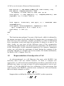
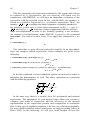
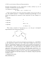
http://www.springer.com/0-387-23158-7 Chapter 2 A CAS AS AN ASSISTANT TO REASONED INSTRUMENTATION Philippe Elbaz-Vincent UMR CNRS & Département de Mathématiques Université Montpellier II, France [email protected] Abstract: We propose to illustrate an approach to reasoned instrumentation with a Computer Algebra System (CAS). We give an overview of how a CAS works (in our case MAPLE), and also some explanations of the mathematical theories involved in the algorithms described. We point out the failures of some methods, and how we can anticipate and prevent them. We conclude by giving some personal insights on how we can use a CAS in an educational framework. Key words: Computation of limits, Computer Algebra System, Reasoned instrumentation, Symbolic integration. 42 Chapter 2 1. PRELIMINARIES 1.1 Foreword Despite the fact that numerous CAS exist, we will work mainly in the present paper with MAPLE (version 5) and DERIVE. Our main interest is in symbolic computation. In such a framework, the software becomes a kind of ‘personal assistant’ for computations and experimentations, for the researcher, as well as the teacher. One of the main problem with a CAS is how to interpret the results, in particular when the computations seem to have gone wrong. In this chapter, we will explore several situations1 which will illustrate what we call reasoned instrumentation, in particular in a classroom context. We will only suppose from the reader some basic knowledge of MAPLE or a similar CAS (e.g., MATHEMATICA, MuPAD or MAXIMA). 1.2 Technical preliminaries It is useful to have a better understanding of how MAPLE (or equivalently your personal CAS) works. In our specific case, we can say that Maple is written in… Maple. Indeed, only ‘basic’ functions are built in another programming language (C in our case). This set of functions is called the kernel of MAPLE. All the other functions and procedures are written using functions from the kernel. This is a great advantage for learning. It is possible to see how most of the functions are written, thus giving us the possibility of modifying them. In order to do this, we use the command interface (verboseproc=2); described in Kofler (1997, Chapter 28). Then, it is enough to print the given procedure in order to see the code. In the following we give three examples: > interface(verboseproc=2): > print(abs); proc() option builtin; 72 end > print(goto); proc() option builtin; 108 end > print(sin); proc(x::algebraic) local n, t; option ‘Copyright (c) 1992 by the University of Waterloo. All rights reserved.‘; if nargs <> 1 then ERROR(‘expecting 1 argument, got ‘.nargs) elif type(x, ’complex(float)’) then evalf (’sin’(x)) A CAS as an Assistant to Reasoned Instrumentation 43 elif type(x| ‘*‘) and member(I| åop(x)ç.) then I*sinh(- I*x) elif type(x, ’complex(numeric)’) then if csgn(x) < 0 then -sin(-x) else ’sin’ (x) fi elif type(x, ‘*‘) and type(op(1, x), ’complex(numeric)’) and csgn(op(1, x)) < 0 then -sin(-x) . . . elif type(x, ’f u n c t i o n ’) and op(0, x) = ’JacobiAM’ then JacobiSN(op(x)) elif type(x, ’arctan(algebraic, algebraic)’) then op(1, x)/sqrt(op(1, x)^2 + op(2, x)^2) else sin(x)¬:= ’sin’ (x) fi end > The functions abs and goto2 are part of the kernel, which is indicated by the option builtin. On the other hand, the function sin is a program of 60 lines and uses other functions. Another possibility in order to understand how a procedure works and what the procedure is doing is to trace it. In other words, we can trace all the different steps of the computation (assuming this functionality was allowed in the procedure). We have access to this functionality via the command infolevel. For instance, infolevel [all]:=5 ; will print the maximum of detail during the running of the procedure and this is a valuable tool for the teacher. For further information, see Kofler (1997: Chapters 28 to 30). 1.3 Representation of an object in a CAS As aforementioned, we will illustrate this topic with MAPLE, but basically most CAS use similar features. In order to compare two expressions, we will need some normalization procedures, particularly in the difficult case where we want to know if a given expression is zero or not. Usually, a CAS like MAPLE does few evaluations of the expressions. But some systems, like DERIVE, perform more evaluations. We can illustrate that on a simple example; we have: 2 3 - 6 = 0. Suppose that we define the variable t, in MAPLE, as the expression: t = 2 3 - 6. 44 Chapter 2 This last expression will return non-evaluated by the system and will not be replaced by 0. Nevertheless, the test is(t=0) will return true. In comparison, with DERIVE, we will have an immediate evaluation of the expression, with the expected result. In fact, with MAPLE, the variable t is stored as a symbolic expression (i.e., a syntactic expression). Thus3, the quantity 2 3 - 6 is nothing else than a sequence of symbols attached to the variable t. In this case, we have three components op(0,t) = +, op(1,t) = 2 3 and op(2,t) = – 6 . Each one of these components could be split into other sub-components, in order to get, formally speaking, a tree structure. An example of normalization, under MAPLE, is given by the command radnormal (for radical normal form). If we apply this command to t, we get: > radnormal(t); 0 This procedure is quite efficient and could simplify (in an algorithmic way) any complex radical expressions. Some examples are given in the following: > radnormal(sqrt(5+2*sqrt(6))); 1/2 1/2 3 + 2 > radnormal(sqrt9^(1/3)+6*3^(1/3)+9)); 1/3 3 + 3 > radnormal((sqrt(3)+sqrt(2))/(sqrt(3)-sqrt(2)), rationalized); 1/2 1/2 5 + 2 3 2 In the last command, we have added the option rationalized in order to normalize the denominators as well. The above operations are consistent with the following equalities: 5+ 2 6 = 3 + 2, + 3, + +9 = 3 + 2 = 5 + 2 6. 3- 2 39 63 3 33 In the same way, there is a normal form for polynomial and rational expressions. The uniqueness of such normal forms allows the system to compare such kinds of expression, and the efficiency of the internal representation of the expressions permits such comparison in reasonable time. In this type of algebraic treatment, CAS are very efficient and reliable. For more details related to radical expressions, we suggest reading Jeffrey & Rich (1999). In the following, we will give some insights on how the A CAS as an Assistant to Reasoned Instrumentation 45 internal representation of the expressions is done, mainly by use of examples. Consider the expression below: > E:=ln(1+x)-2*sin(1+x); E¬:=ln(1 + X) - 2 sin(1 + x) From a user point of view, the expression could be seen as a tree with, as root, the dyadic operator +. Using the commands op and nops , we can explore the apparent tree structure of the expression. In our example, we have: > nops(E); 2 > op(0,E); + > op(1,E); ln(1 + x) > op(2,E); -2 sin(1 + x) Thus using a sequence of op(op(op(…))) , we can get a conceptual representation of the expression as below: + ln * + 1 * x 2 sin -1 + 1 x Nevertheless, this is not the true internal representation (i.e., in MAPLE) of the expression, which is in fact a little more complex but also more efficient. Technically speaking, the model for the internal representation is what is called a DAG4, which allows the elimination of any common subexpression (i.e., we only represent, and compute, once any given subexpression which appears several times inside the main expression). It is difficult to see directly this representation in MAPLE. However, using the command dismantle (which we need to load with readlib(dismantle)), we can get a glimpse of the DAG structure. For instance, using our previous example, we get: > dismantle[dec](E); SUM(136478368,5) 46 Chapter 2 FUNCTION(136040888,3) NAME(135425704,4): ln #[protected] EXPSEQ(136609520,2) SUM(135549672,5) INTPOS(135407372,2): 1 INTPOS(135407372,2): 1 NAME(135426280,4): x INTPOS(135407372,2): 1 INTPOS(135407372,2): 1 FUNCTION(135443776,3) NAME(135426680,4):sin # [protected] EXPSEQ(136609520,2) SUM(135549672,5) INTPOS(135407372,2): 1 INTPOS(135407372,2): 1 NAME(135426280,4): x INTPOS(135407372,2): 1 INTNEG(135407380,2): -2 The option dec allows us to identify the memory address (inside MAPLE) of the objects. For instance, an expression of the type SUM(135549672,5) means that we have a sum and its result will be put at the (memory) address 135549672. As we can see, the quantity 1 + x is put at this address and thus is computed only once. And so is ln(1 + x) (at the address 136040888). If another procedure uses this quantity, then it will point to this address. In order to understand this notion, we will digress slightly, and use a simple example: > B:1n(1+x)^2; 2 B¬:= ln(1 + x) > dismantle [dec](B); PROD(136082120,3) FUNCTION(136040888,3) NAME(135425704,4): ln # [protected] EXPSEQ(136609520,2) SUM(135549672,5) INTPOS(135407372,2): 1 INTPOS(135407372,2): 1 NAME(135426280,4): x INTPOS(135407372,2): 1 INTPOS(135407388,2): 2 No surprise there; the variable B ‘points’ to the expression ln(1 + x) previously defined in E. If we set x : = 3, since it is an integer we should have an immediate evaluation and B should be equal to ln(4)2; but doing so, B will point to a new address. Here is the session: A CAS as an Assistant to Reasoned Instrumentation 47 > addressof(B); 136082120 > B; 2 ln(1 + x) > addressof(x); 135426280 > x:=3; x¬:= 3 > addressof(x); 135407404 > B; 2 ln(4) > addressof(B); 136154348 > E; ln(4) - 2 sin(4) > dismantle [dec](B); PROD(136154348,3) FUNCTION(136154236,3) NAME(135425704,4): ln # [protected] EXPSEQ(135824692,2) INTPOS(135407420,2): 4 INTPOS(135407388,2): 2 > dismant1e [dec] (E); SUM(135484800,5) FUNCTION(136154236,3) NAME(135425704,4): 1n # [protected] EXPSEQ(135824692,2) INTPOS(135407420,2): 4 INTPOS(135407372,2): 1 FUNCTION(136324224,3) NAME(135426680,4): sin # [protected] EXPSEQ(135824692,2) INTPOS(135407420,2): 4 INTNEG(135407380,2): -2 We have used implicitly the command addressof in order to get the (memory) address of a MAPLE object (which we can see in the printing of dismantle). As we can see, the structure of the expression is left unchanged (B is still a sub-expression of E, and the DAGs are unchanged too), but the addresses have changed. As a matter of fact, MAPLE (as other CAS) uses an internal table for its objects, which maps each object to an address. When the value of an object changes, the table of addresses is updated, but losing the expressions already present in the memory. In our example, the address 48 Chapter 2 which corresponds to the expression ln(1 + x) is still there. Indeed, if we revert x to being a formal variable, we get our initial values: > x¬:= ’x’; x¬:= x > E; ln(1 + x) - 2 sin(1 + x) > B; 2 ln(1 + x) > addressof(E); 136478368 > addressof(B); 136082120 This illustrates the value of the DAG representation and its efficiency. Its downside is the memory consumption. The reader will find further discussions of this topic in Giusti & al (2000) and at the end of Chapter 2 of Gomez & al (1995) and in Nizard (1997). As a final point, we will show5 how the DAG structure is suitable for computing formal derivation of an expression. Suppose we want to differentiate (formally) the symbolic expression: x 2 2 x g(x) = 2xe sin(e ) . Its DAG representation is given by: a 1 = x, a 2 = a 21 , a 3 = e a2 , a 4 = sin(a 3 ), a 5 = a 3a 4 , a 6 = a1a5 , a 7 = 2, a 8 = a 7a 6 . Then, we get the derivative of g by a formal derivation of each node of the DAG, resulting in a new DAG which is the associate to the derivative of g (say, with respect to x). If we denote by , this formal derivation, then using the basic rules, we have: A CAS as an Assistant to Reasoned Instrumentation 49 ,a 1 = 1, ,a 2 = 2a 1 ,a 1 , ,a 3 = ea 2 ,a 2 , ,a 4 = cos(a 3 ),a 3 , ,a 5 = a 3 ,a 4 + a 4 ,a 3 , ,a 6 = a 1 ,a 5 + a 5 ,a 1 , ,a 7 = 0, ,a 8 = a 7 ,a 6 + a 6 ,a 7 We should notice the technical simplicity of this approach, which is independent of the choice of DAG structure. Despite the fact that our data structure is efficient, it does not mean that we can always show that something which should be zero is really zero. In the same way, we cannot put all the ‘special identities’ in the CAS. For instance, in MAPLE, the expression sin2 x + cos2 x = 1 is not ‘equal’ to l, even if x is assumed to be a real number. On the other hand, simplify ‘knows’ the identity: > restart; > a:=cos(x)^2+sin(x)^2; 2 2 a¬:= cos(x) + sin(x) > is(a=1); FAIL > eval(a); 2 2 cos(x) + sin (x) > assume(a,real):eval(a); 2 2 cos(x~) + sin(x~) > x¬:= ’x’:simplify(a); 1 But other (in fact most) well known identities cannot be reduced (even with simplify). > restart; > b:=arccos(x)+arcsin(x); b¬:=arccos(x) + arcsin(x) > simplify(b); arccos(x) + arcsin(x) But, we can use MAPLE to investigate this identity. > diff(b,x); 0 50 Chapter 2 > eval(subs(x=0,b)); 1/2 Pi As a general fact, the procedures of normalization or simplification are rather limited. On one side, we cannot put all the ‘special identities’ in a computer, and on the other we often have multiple choices for the simplification (technically, speaking it is a rewriting problem). From a theoretical point of view, we have a kind of decidability limitation. Indeed, Richardson (1968) has shown that for the class R defined as the closure of rational functions of Q (p, ln(2), x) under the action of sine, exponential and absolute value maps, the predicate E = 0 is ‘recursively indecidable’ for E Œ R. Here the notion of decidability is relative to the theory of formal languages and grammars. A variation of this result to symbolic integration is given in Davenport & al (1987, p.168). In practice, this is far less limiting than we might imagine. First, a lot of functions belong to a class for which decidability is established, and furthermore, there exist probabilistic methods which can be used efficiently in such settings. Nevertheless, this shows that a ‘perfect’ CAS, able to simplify ‘ideally’ any expression is a pure dream. 2. BASIC COMPUTATIONS AND LIMITS While the main target users of a tool such as DERIVE are at high school level, this is quite different for MAPLE and other general CAS, which are designed for the engineer, the scientist and the researcher. Thus, such software is designed with generality in mind, and this can have some undesirable side effects for the student. We give a concrete example below: > f:=x->evalf(x^(1/3)); 1/3 f¬:=x -> evalf(x ) > f(-1); .5000000000 + .8660254038 I In general, and as seen in the classroom by the author, the student expects to get f(–1) = –1. But, the explanation is quite simple; it is enough to think complex! Indeed, if we search for a solution of the form eiq, we p reasonably get q = 3 , and it is this solution that the CAS gives. Most of the system operates, by default, on the complex numbers, as is also the case for advanced pocket calculators. Thus, we should show some caution when we use these tools, in particular in the classroom. Most of the time, problems A CAS as an Assistant to Reasoned Instrumentation 51 can be solved by giving some help to the system. Here is a simple example: let a be a positive real number, and p an arbitrary real number. Set: 2 p b = log ( ap+1) a a Taking account of the hypothesized characteristics of a and p, we should have b = p2 – p – 1. But the expression is not simplified into this form by MAPLE, mainly due to the fact that, for the system, a and p are complex numbers. We need then to make our further assumptions clear to the system: > b:=log[a]((a^p)^p/a^p/a); p p (a ) ln (------) p a a b¬:= ---------ln(a) > simplify(b); p p (-p -1) ln((a ) a ) ------------------ln(a) > assume(a>0); > simplify(b); (p - 1) p ) ) -ln(a˜) + ln((a˜ -----------------------ln(a˜) > assume(p,real); > simplify(b); 2 p˜ - p˜ -1 2.1 Computation of Limits Taking limits of functions or of sequences is one of the most important notions of analysis. Hence, the behavior of CAS in this particular area is of prime interest. Several approaches have been developed to perform this kind of computation, and they are detailed in the works of Gruntz (1996, 1999). The first approach is what we can call the ‘heuristic method’. In short, we use as main tool the Bernouilli de l’Hôpital rule6 (which we will denote by BdH in the remainder of the text). The heuristic involves deciding how many iterations of the rule will be applied. Unfortunately, this method has several gaps. First of all, there are many types of expression which remain difficult to compute after applying the BdH rule, and furthermore, applying 52 Chapter 2 BdH could increase the complexity of the expressions and thus the computations. The second approach consists of using power series expansions (mainly Taylor expansions). This method is quite systematic, but it fails when: - a zero expression is not detected by the system as being zero; - there are an infinity (or at least a ‘huge number’) of zero terms in the power expansion. Such a situation appears when we compute the sum of functions, which could result in infinite cancellations; - there are one or several parameters in the expression. The first point, as already discussed, is very difficult in practice (Gruntz 1996, § 7.2; 7.3). A possible solution, depending of the type of expression, is to redefine the zero test used by the CAS. For instance, with MAPLE, it is done via the command Testzero, which by default uses the standard normalization procedures. An example is given later. Another possibility is to use some probabilistic method to perform the test. The second point is well known to undergraduate students and is mainly related to the order of the power expansion; several methods exist to deal with this problem. The last point is more difficult in practice, and will mostly require use of heuristics. To the best of our knowledge, DERIVE (and so the TI-92) uses a heuristic approach for the computation of limits, while MAPLE uses power series expansion methods. As we will test out below (and as we can see in the examples given in Wester 1999, p.166 and 168), CAS are quite fragile on limit computations. It is likely that the teacher (and the user) will need to take a lot of precautions, and in particular will need to know what to expect from the system. This is a typical situation where reasoned instrumentation is important. We will now give several examples from a MAPLE session (in command line), that we will explain in detail at the end, and we will conclude by a discussion of the numerical approach to limit computations. Most of the following examples are extracted from or inspired by Wester (1999) and Gruntz (1996). > > > > # Example 1 restart; # problem of the order limit((sin(tan(sin(x)^7))-tan(sin(sin(x)^7)))/x^49,x=0); 7 7 sin(tan(sin(x) ))- tan(sin(sin(x) )) lim -----------------------------------x -> 0 49 x > Order; 6 A CAS as an Assistant to Reasoned Instrumentation > Order:=50; Order¬:= 50 > limit((sin(tan(sin(x)^7))-tan(sin(sin(x)^7)))/x^49,x=0); -1 -30 > # Example 2 > restart; > A:=(sqrt(8)*(arccos(1/3+h)-arccos(1/3))/3/h)^2; 2 (arccos(1/3 + h) - arccos(1/3)) A¬:=8/9 -------------------------------2 h > limit(A,h=0); infinity > series(A,h=0,1); 2 -2 8/9 (1/2 Pi - arcsin(1/3) - arccos(1/3)) h 1/2 -1 4/3 (1/2 Pi - arcsin(1/3) - arccos(1/3)) 2 h + 1/2 (-1/4 (1/2 Pi - arcsin(1/3) - arccos(1/3)) 2 +1) + 0(h) > # most of the terms in the above expression should be zero! > # Example 3 > restart; > A¬:=ln(h)/(ln(h)+sin(h)); ln(h) A¬:= --------------ln(h) + sin(h) > limit(A,h=infinity); infinity > series(A,h=infinity,2); > Error, (in asympt) unable to compute series > A1:=1/(1+sin(h)/ln(h)); 1 A1¬:= ---------sin(h) 1 + -----ln(h) > limit(A1,h=infinity); infinity > limit(1+sin(h)/1n(h),h=infinity); 1 > # this is in fact a problem of operations on the limit! > > # Example 4 > restart; > C:=z/(sqrt(1+z)*sin(x)^2+sqrt(1-z)*cos(x)^2-1); 53 54 > > > > > > > > > > > > > > > > Chapter 2 z C¬:= ------------------------------------------1/2 2 1/2 2 (1 + z) sin(x) + (1 - z) cos(x) - 1 limit(C,z=0); 0 # wrong result¬! # trying to explain the behavior series(C,z=0,2); 1 2 -------------------- z + 0(z ) 2 2 sin(x) + cos(x) - 1 # the coefficient in z is in fact infinity! # it is again a problem of testing equality to zero # Here is a way to solve the problem via some re-writing restart; Testzero:=t -> evalb(normal(convert(t,exp))=0); Testzero¬:= t -> evalb(normal(convert(t, exp))=0) C:=z/(sqrt(1+z)*sin(x)^2+sqrt(1-z)*cos(x)^2-1); z C¬:= ----------------------------------------1/2 2 1/2 2 (1 + z) sin(x) + (1 -z) cos(x) - 1 limit(C,z=0); 2 ---------------2 2 sin(x) - cos(x) # correct result! # Example 5 restart; F:=(ln(x)^2*exp(sqrt(ln(x)*ln(ln(x))^2\ )*exp(sqrt(ln(ln(x)))*ln(ln(x)))^3))/sqrt(x); 2 1/2 2 1/2 3 1n(x) exp(ln(x) ln(ln(x)) ) exp(ln(ln(x)) ln(ln(ln(x))) ) F:= ------------------------------------------------------x 1/2 > limit(F,x=infinity); 0 > # which is also correct. Comments Example 1 illustrates the classic problem of ‘guessing’ in which order we need to perform the power series expansion in order to remove the indeterminate form. We should notice that computing the power series expansion at the start with a systematically large order is costly in terms of running time, and we also need to take this into account. A CAS as an Assistant to Reasoned Instrumentation 55 Example 2 is a ‘test to zero’ problem. The limit computed by MAPLE is incorrect. In order to understand what is going on, we do a power series expansion, and we notice that the method fails because the classical relation: p 1 1 = arccos + arcsin , 2 3 3 is not know by the system (cf. previous section). In theory, the power series expansion should look like: series(A,h = 0,1) = 1+O(h), and we should conclude that the limit is 1 (correct answer). Both examples are correctly computed by DERIVE (TI-92), and as an exercise for the reader, we can check (with MAPLE for instance) that both limits can be performed with the BdH rule. Example 3 is of a different type. Indeed, it is straightforward to show that the limit is equal to 1. Surprisingly enough, DERIVE gives the correct answer. But MAPLE fails due to the asymptotic expansion of the expression (it is the sine which is the culprit here). Transforming the expression does not help, despite the fact that MAPLE can compute easily that: sin(h) lim (1+ ln(h) ) = 1 . hÆ +• This is in fact a simple problem of operations on the limits. Since the limits of the numerator and denominator exist and are equal to 1, it should be possible to conclude that the limit of the expression is 1. Again, DERIVE computes this limit correctly, most likely by performing some basic operations on the limit. Example 4 is of the same type as Example 2. The classical relation sin2 x + cos2 x = 1 is not known by the system and generates a singularity in the power series expansion. Here, the proposed solution is a modification of the “test to zero”, by reprogramming the procedure Testzero with a more suitable normalization. Then, the computation can be done correctly. We should notice that we can get the limit directly via BdH, and thus DERIVE gets the correct answer immediately. However, if in the expression C we replace x by 1/x and z by exp(–x), with x Æ + , then MAPLE gives a correct answer, namely –2, while DERIVE is unable to evaluate the expression. Example 5 is straightforward for MAPLE, but is unsolved by DERIVE which remains in “Busy” position. It is in fact a typical example of a limit which is cumbersome for the heuristic approach. We can check that most of the limits (Wester 1999, p.166 and 168) are difficult for DERIVE. 56 2.2 Chapter 2 Numerical limit vs. Symbolic limit We might think that the computation of limits should be easily done via numerical evaluation of the function in the neighborhood of the point, which could be given by a numerical sequence of points in this neighborhood. This possibility is indeed implemented in MAPLE, and can be called by the command evalf(Limit()). For examples 2 and 1, we get: > restart; > A:=(sqrt(8)*(arccos(1/3+h)-arccos(1/3))/3/h)^2; 2 (arccos(1/3 + h) - arccos (1/3)) A¬:=8/9 ---------------------------------2 h > evalf(Limit(A,h=0)); 1.000000000 > evalf(Limit((sin(tan(sin(x)^7))- tan(sin(sin(x)^7)))/x^49, x=0)); Error, (in evalf/limit/levinu) invalid cancellation of infinity As we can see, while we get a correct answer for Example 2, Example 1 is still problematic. In the same way, it is difficult to get a numerical estimate of the limit at infinity of a general function. Furthermore, new problems could arise, as shown with the example below (Gruntz 1996, p.4-7). > restart; > C¬:=1/x^(ln(ln(ln(ln(1/x))))-1); 1 C¬:= -------------------------(1n(1n(1n(1n(1/x)))) - 1) x > evalf(subs(x=10^(-3),C)); .00005602749469 > evalf(subs(x=10^(-6),C)); -6 .6146316300 10 > evalf(subs(x=10^(-12),C)); -9 .1528656745 10 > evalf(subs(x=10^(-24),C)); -16 .7787481717 10 > evalf(subs(x=10^(-80),C)); -39 .1401026662 10 > # Is the limit 0...? >¬# 10^80 is quite close to the number of atoms in universe... > our A CAS as an Assistant to Reasoned Instrumentation 57 > limit(C,x=0,right); infinity > # oops¬! > A plot of the function would confirm the ‘numerical evidence’, but the result given by the symbolic procedure is in fact correct (Exercise left to the reader). Even increasing the number of digits will not change the numerical evaluation. Indeed, for 1/x large (e.g., 1080), the iteration of ln diminishes tremendously the effect of 1/x and thus the expression C behaves almost as x1-e with ‘ e small’, which gives evidence for the ‘limit 0’. But, in order to ee suppress the effect of the iteration of ln, we need to take x < e-e , or say x smaller than 10-1656521…(sic!) 3. SYMBOLIC INTEGRATION This is one area where the CAS is a genuinely valuable tool. Due to the ubiquity of integration, both in mathematics and the sciences in general, we often have to perform antiderivation (i.e., symbolic integration) in order to solve the problem. For several years, physicists and engineers had to use huge tables of antiderivatives, also well known to contain several errors. But CAS are particularly efficient in this task, due to the fact that we have reasonably efficient algorithms, which are consequences of mathematical results often deep and unknown to most mathematicians. The goal of this section is to describe the methods, and give some examples of reasoned instrumentation. We heartily suggest that the reader look at Davenport & al (1987, Chapter 5) for further investigations. Usually, the hand computation of antiderivatives is strongly based on heuristics (inherited from personal knowledge) such as: use of tables, change of variables, integrating by parts, use of multidimensional integrals, and so on. As pointed out in Gomez & al (1995, Chapter 9, p.227): “These methods often allow us to find an antiderivative quite quickly, but if they fail you cannot conclude”. The methods used by the CAS are both heuristic and algorithmic. The result depends strongly on the type of function that we are integrating. In particular, for a given class of functions, a failure of the procedure is in fact a proof that the antiderivative cannot be expressed in terms of ‘elementary’ functions. We will begin by giving definitions and explain the practical difficulties. We will mainly follow the approach of Davenport (1987, Chapter 5, § 5.1.3). 58 Chapter 2 Definition 3.1 Let K be a field of functions over a field k (not necessarily a prime field). The function q is said to be an elementary generator on K if one of the following conditions holds: 1. the function q is algebraic over K (i.e., satisfies a polynomial equation with coefficients in K); 2. the function q is exponential over K (i.e., for a k-derivation D of K, there exists a e K such that D(q) = D(a)q); 3. the function q is logarithmic over K (i.e., for a k-derivation D of K, D(a) there exists a e K such that D(q) = a ). Remark 3.2 Despite the fact that we can take a ‘k-derivation’ in a general sense (i.e., an element of Derk(K)), in practice K = k(t1,…,tn) and D = ,t, for a certain i, i where the tl are indeterminate. In order to get an elementary generator which is not algebraic over K, we add formally the element exp(u) with the rules of derivation of the exponential (idem for the log). Now we can introduce the following notion. Definition 3.3 Let K be a field of functions over the field k. A field K(q1,…, q n) containing K is called a field of elementary functions over K if each q i, i = 1,…,n, is an elementary generator over K. A function is said to be elementary over K if it is an element of a field of elementary functions over K. A result of Liouville, often called ‘Liouville’s principle’, gives the general form of the primitive of an element of a function field K if the function is elementary over K. The crucial result which is used and its algorithm implemented in most CAS is the theorem of Risch (Davenport & al 1987, p.185). Theorem 3.4 (Risch 1969) Let K = k(x, q1,…, qn) be a field of functions over k. We suppose that each qi+1 is either a logarithm, or the exponential of an element of k(x, q1,… qi), and is transcendental over this field. Then there exists an algorithm which, given an element f of K, either gives an elementary function on K which has f as derivative, or proves that f does not admit an elementary antiderivative on K. This result illustrates the fact that a ‘failure’ gives non-trivial information about the problem. The proof of the theorem of Risch is understandable at the undergraduate level. To the best knowledge of the author, the algorithm A CAS as an Assistant to Reasoned Instrumentation 59 of Risch implemented in MAPLE is only complete for the class of elementary functions which are purely transcendental (no algebraic dependency involved; for instance arcsin is not purely transcendental). Thus we can apply the theorem of Risch only to this class of functions. For further reading we suggest (Davenport 1987, § 5.1.8) and (Bronstein 1990, 1997). In practice, particularly in the classroom, the main difficulty will be to understand that a simple modification of the expression to be integrated will result, most of the time, in an antiderivative quite different in appearance. We will give some examples below: > diff(sqrt(4^x+1),x); x 4 ln(4) 1/2 ----------x 1/2 (1 + 4 ) > f1:=int(4^x/sqrt(1+4^x),x); x 1/2 (1 + 4 ) f1¬:=2 ------------ln(4) > # Here Maple identifies the derivative > # Let us change 4^x to 2^(2*x) > > f2:=int(2^(2*x)/sqrt(1+4^x),x); infinity -----\ _k2 f2¬:= 2 ) GAMMA (_k2 + 1/2) (-1) / -----_k2 = 0 / / 1n(2) \\ // |1 - exp(- 1/2 x (1n(4) + 2 _k2 ln(4)) |1 - 4 -----------------|)|/| \ \ / ln(4)¬+¬2¬_k2¬1n(4)// /\ ln(2) \\ / GAMMA(_k2 + 1 (1n(4) + 2 _k2 1n(4)) |1 - 4 ------------------|| / \ ln(4) + 2¬_k2 ln(4)// / 1/2 Pi > # oops¬! > # Compare the two results ... > evalf(series(f2,x)); 2 3 4 .7071067812¬x¬+¬.3675968038¬x ¬+¬.09908837872¬x ¬+¬.01103831202 x + 5 6 .00008501305392¬x ¬+¬0(x ) > evalf(series(f1,x)); 60 Chapter 2 2 3 2.040278892¬+¬.7071067810¬x¬+¬.3675968036¬x ¬+¬.09908837866¬x ¬+ 4 5 6 .01103831201¬x ¬+¬.00008501305389¬x ¬+¬0(x ) > Digits; 10 > Digits:=20; Digits¬:= 20 > evalf(series(f1,x)); 2.0402788931935789636¬+¬.70710678118654752440¬x¬+¬.3675968038007051968 2 3 4 9¬x ¬+¬.099088378720063520381¬x ¬+¬.011038312018296660770¬x ¬+ 5 6 .000085013053929147665047 x ¬+¬0(x ) > evalf(series(f2,x))¬; 2 .70710678118654752440¬x¬+¬.36759680380070519690¬x ¬+¬.0990883787200635 3 4 5 20388x ¬+¬.011038312018296660770x ¬+¬.000085013053929147665054x ¬+¬ 6 0(x ) > In the above example, we can see the practical difficulty of antiderivative computations. We can check that the results are the same up to a constant 2 (which is exactly 1n(2) ). In a classroom situation, without the help of the teacher, it is likely7 that the students will claim failure of the software and will stop there. Here, the theorem of Risch says that we should anticipate a correct result. Nevertheless, we can try to do some manipulations, in order to see if we can avoid such difficulties: > Q¬:=2^(2*x)/sqrt(1+4^x); (2 x) 2 Q¬:= --------x 1/2 (1 + 4 ) > simplify(Q); x 4 ---------x 1/2 (1 + 4 ) > QQ:= normal (Q, expanded); x 2 (2 ) QQ¬:= --------x 1/2 (1 + 4 ) > int(QQ,x); (2 x) 1/2 (1 + 2 ) --------------ln(2) A CAS as an Assistant to Reasoned Instrumentation 61 As we can see, using simplify gives the original form of the expression. Furthermore, the normalization with the option expanded, results in an even simpler expression for the antiderivative. It could be wise to develop such an approach, by using normal for instance, in order to get a ‘good’ expression before integration. Here are other illustrations of the theorem of Risch: > int(1/ln(x^2+1),x); / | 1 | --------- dx 2 | ln(x + 1) / This shows, assuming no errors in the software or the hardware, that 1 has no elementary antiderivative, as this function is purely ln(x2 +1) transcendental. But the situation is less simple, with non purely transcendental elementary functions. Here is an example from Gomez (1995, p.235-236): > f3:=int(arcsin(x)^2,x); / | 2 f3¬:= | arcsin(x) dx | / But this is a classic antiderivative. We need to help the system. For this purpose, we can do an integration by parts using the package student. > intparts(f3,arcsin(x)^2); / | 2 arcsin(x) x 2 arcsin(x) x - | 2 ------------ dx 2 1/2 | (1 - x ) / > intparts(%,arcsin(x)); / | 2 2 1/2 arcsin (x) x + 2 arcsin(x) (1 - x ) + | -2 dx | § 62 Chapter 2 > value(%); 2 2 1/2 arcsin(x) x + 2 arcsin(x) (1 - x ) - 2 x Hence, by interacting with the CAS, we get a correct answer. This indicates the right way to use a CAS, and it is what the student will have to learn. 3.1 Difference between antiderivative and indefinite integral Another aspect, often neglected, is the study of the result of the computation of an antiderivation. Indeed, in the usual settings, we want to compute a definite integral of a function which in most cases will be continuous on the interval of integration. Thus, we expect the antiderivative of the function integrated to also be continuous (and even more). Unfortunately, in many cases, it is not. As we have seen in the previous section, the computation of the antiderivative is a purely algebraic process. We just ask to find an element g of a differential field such that D(g) = f for the derivation D of the field. On the other hand, in a classical course on integration, we introduce the notion of indefinite integral of a function (real or complex variable), which is often confused with the notion of antiderivative. To be more precise, we will give a definition of this notion: Definition 3.5 (Jeffrey 1994, p.35) An indefinite integral of a function f, Lebesgue-integrable on an interval I of R, is any function G defined on I and a real number c, such that: x G(x) = Úa f(t)dt + c . One of the main results of undergraduate courses in calculus (Riemann rather than Lebesgue) is that the indefinite integral is an antiderivative of f. But if f is continuous on I, so is G. However, an antiderivative is not necessarily an indefinite integral, and the CAS gives us several examples: > int(6/(5-3*cos(x)),x); 3 arctan(2 tan(1/2 x)) Here the result is an antiderivative on R, but fails to be continuous. As a consequence, we cannot use this antiderivative ‘out of the box’, in order to compute the definite integral of the function on [0,4p] for instance. The result would be nonsense (but apparently most students are not afraid of that). Nowadays, new heuristics and algorithms try to produce better results, closer to an indefinite integral; Jeffrey (1994) for more details. A CAS as an Assistant to Reasoned Instrumentation 4. 63 CONCLUSION The main point that we have tried to establish, through several examples, is that we cannot reasonably use a CAS as a black box, in particular in the classroom. Teachers should have sufficient knowledge of the behavior of the CAS in order to understand the result for themselves, and also for their students. Working with a computer always involves a risk. But, while students will accept a system or hardware failure, they will be less inclined to accept failure from the teacher, which will undoubtedly undermine the often fragile trust between them. We should also take into account that a student will often use ‘the’ worst possible strategy in order to solve a problem; in general, this will require the teacher to improvise in order to explain either the failure or the success of the strategy. This provides further evidence that teachers need a sufficient knowledge of the CAS if they want to ‘feel in control’ in the computer classroom. Furthermore, many teachers have generally accepted ideas about the CAS (and using CAS in the classroom) which could work against them. One of the most prominent ideas is the belief that working with a CAS means teaching (and training) the students how to compute (as in the classical first undergraduate courses on calculus and algebra). Unfortunately, as already seen in the examples discussed in this paper, this is not true. Indeed, students need to acquire enough practical experience to develop insight on the methods learned. For instance, this will help them to estimate the order needed to compute a limit using power series expansions of composed functions, or the transformations to perform in order to compute an antiderivative. On the other hand, computing the power series expansions of functions up to a high order as the climax of a calculus course is pointless. This is why we believe that a reasoned instrumentation should be preferred when we have to use CAS in the classroom. The ‘intelligent usage’ of a CAS in mathematical science courses (or in other sciences) is not an easy task, and in particular is not given. This implies the necessity of developing specific classroom activities and specific exercise sheets, well adapted to the task, showing clearly the value of the CAS either as a platform for experimentation or as an assistant, and well integrated into the main course. Philippe ELBAZ-VINCENT ([email protected]) is an assistant professor at the Université Montpellier II (France). His research area is algebra and number theory, in which he develops computational methods. 64 Chapter 2 NOTES 1. The examples given have been produced with the version V release 5.1 of MAPLE under GNU/LINUX-2.4 (architecture i686) and SOLARIS 5.8 (architecture Ultrasparc II) and with the DERIVE version implemented on the TI-92 pocket calculator (Texas Instruments). 2. This last function is undocumented… 3. We can access the components of this expression via the command op, and nops to get the number of components (as coded by MAPLE). 4. Directed Acyclic Graph. 5. Based on an example from Ole Stauning for the software FADBAD of automatic formal derivation. 6. The famous rule of the Marquis de l’Hôpital (1661-1704) is in fact due to Johan Bernoulli, 1667-1748, cf. (http://www-groups.dcs.st-andrews.ac.uk/~history/Mathematicians/Bernoulli_Johann.html). 7. As experienced several times by the author. A Cas as an Assistant to Reasoned Instrumentation 65 REFERENCES Bronstein M. (1990) On the integration of elementary functions, Journal of Symbolic Computation 9(2), 117-173. Bronstein M. (1997) Symbolic Integration I - Transcendental Functions, Algorithms and Computations in Mathematics (Vol. 1). Heidelberg: Springer-Verlag. Crandall R.E., Mayer E.W. & Papadopoulos J.S. (1999) The twenty-fourth Fermat number is composite, preprint. Davenport J., Siret Y. & Tournier E. (1987) Calcul formel: systèmes et algorithmes de manipulation algébrique. Paris: Masson. Dumas P. & Gourdon X. (1997) Maple: son bon usage en mathématiques. Berlin: SpringerVerlag. Fortin P. Introduction au calcul formel. Paris: Texas Instruments. Giusti M., Hägele K., Lecerf G., Marchand J. & Salvy B. (2000) Computing the Dimension of a Projective Variety: the Projective Nœther Maple Package, Journal of Symbolic Computation 30(3), 291-307. Gomez C. Salvy B. & Zimmermann P. (1995) Calcul formel: mode d’emploi, exemple en Maple. Paris: Masson. Gruntz D. (1996) On computing Limits in a Symbolic Manipulation System, Ph.D Thesis ETHZ. Gruntz D. (1999) Computing Limits in Computer Algebras Systems, in M.J. Wester (Ed.), Computer Algebra Systems: A practical guide (pp. 153-170). Wiley. Jeffrey J.D. (1994) Integration to obtain expressions valid on domains of maximum extent, in M. Bronstein (Ed.), Proceeding of ISSAC 93 (pp. 34-41). ACM Press. Jeffrey J.D. & Rich A.D. (1999) Simplifying Square Roots of Square Roots by Denesting, in M.J. Wester (Ed.), Computer Algebra Systems: A practical guide (pp. 61-72). Wiley. Kamerich E. (1998) A Guide to Maple. New York: Springer-Verlag. Kofler M. (1997) Maple: An Introduction and Reference. Addison Wesley. Lazarus A.J. (1994) Implications of Computational Mathematics, in W. Gautschi (Ed.), Mathematics of Computation 1943-1993: A Half-Century of Computational Mathematics, Proceeding of Symposia in Applied Mathematics 48 (pp. 561-564). AMS. Nizard A.F. (1997) Structure des objets Maple, exposé stage de Luminy, option Info des classes de prépa, CIRM (http://pauillac.inria.fr/~quercia/documents-info/Luminy97/nizard/articl97.ps). Plestsch B. (1999) Computer Algebra in Mathematics Education, in M.J. Wester (Ed.), Computer Algebra Systems: A practical guide (pp. 285-322). Wiley. Richardson D. (1968) Some Undecidable Problems Involving Elementary Functions of a Real Variable, The Journal of Symbolic Logic 33(4), 414-520. Trouche L. (1998) Expérimenter et prouver: faire des mathématiques au lycée avec des calculatrices symboliques. Montpellier: IREM, Université Montpellier II. Von zur Gathen J. & Gerhard J. (1999) Modern Computer Algebra. Cambridge University. Wester M.J. (Ed.) (1999) Computer Algebra Systems: A practical guide. Wiley.