1
AFM Simple User's Guide V2.1 April 2008
A. Mounting the tip
1. Place the tip holder in the black base by holding the release button down,
sliding the two pins into place and fixing it by releasing the button.
2. Loosen the middle screw on the tip holder using a small Philips (+)
screwdriver.
3. Remove the old tip if it is still in place using sharp tweezers.
4. Select your new tip according to your experiment (USERS OUTSIDE the
Molecular Mechatronics Lab SHOULD BRING THEIR OWN TIPS!)
5. Bring the tip over the tip holder using tweezers. The tip must be held above
the clear face of the small prism on the tip holder, not the frosty ones.
6. Slide the back edge of the tip under the metal holder.
7. Nudge the tip slightly to the left and right by the tweezers. As the quartz
surface underneath is slightly inclined, this will result in the tip sliding back
into place until it hits the back groove of the holder. If you lift the tip during
this process, it may slip over the groove and go too far.
Figure 1: Side view schematic of the AFM tip holder
8. Tighten the middle screw. Don't tighten too much. It should be tight enough
such that if you push it with the tip of the tweezers with the weight of your
hand, it shouldn't move.
B. Mounting the tip holder into the head
DON'T TOUCH THE TIP during this process!
1
2
1. Lift the head with both hands and place it on its right side on the metal shelf
inside the chamber.
2. Turn the controller OFF to prevent accidentally shorting the electrical
connections on the head and the tip.
3. Hold the tip holder with one hand and bring it right above its place.
4. Press the black release button with your other hand and hold it down.
5. Push the tip holder down and slide slightly, such that the two grooves on its
sides engage with the two pins on the head. Push the tip holder in place.
6. Release the black button.
7. Hold the tip holder by putting your fingers on its two sides and shake it
gently to assure it has been mounted properly.
8. Turn the controller back ON.
3
C. Tip Alignment
1. Start the MFP3D software
2. Place the head upright on its three legs on the metal shelf. Place the IR
laser sensor card underneath the head
3. Turn on the laser on the controller panel by turning the key.
4. Find the laser spot on the IR card. If the spot dims, move the card to refresh
the intensity.
5. Make sure the spot is sharp. If the spot is fuzzy even when you move the
sensor card, it means that the laser is passing through the frosty glass sides
of the prism. Turn LDX to adjust.
6. Bring LDY to the middle of its range (LDY turns for ~8 full turns from one
end to the other). Turn LDX until the spot suddenly disappears. This is
where the edge of the tip is.
7. Turn LDY until you see a small shadow passing through the spot.
8. By looking at the sum and deflection monitors in MFP3D program,
maximize 'Sum' by slightly adjusting LDY and LDX consecutively. (For an
AC240 tip and most tapping mode tips around, a SUM of > 5 is enough and
need not be maxed)
9. Turn the PSD wheel to adjust and minimize the "Deflection"
D. Head Alignment
1. Place your sample on the stage and fix it using the two magnets.
2. Place the head on the stage: Place the two hind legs in the two holes and
lower the front leg slowly to insert it into place. Keep your eyes on the tip
and make sure that it does not touch the sample as you lower it. If it looks
too close to the sample, raise the head by turning the wheel on its front in
the direction labeled 'Up'.
3. Make sure that when the head is placed on the stage, the 'Vertical position
Indicator' on the vibration isolation table rests in the middle of its range,
marked by a white line. If it is lower or higher, turn the 'Load Adjust' handle
on the table's front to adjust the load, such that it is balanced.
E. Sample Alignment for 'Top Optics' (For bottom optics consult
Tissa)
1. Turn on the optical microscope illumination. Turn on the video by clicking on the
video icon in MFP3D at the bottom left hand side of the screen.
2. Adjust the camera position using the two small knobs at the back of the head.
3. Focus the camera using the wheel that is enclosed in the column under the two
small knobs.
4. The illumination level can be adjusted using either the 'fibre-Lite' remote
intensity control. The diaphragm aperture can be adjusted by the knob on the
side of the stage.
5. The two large knobs on the left side of the stage move the whole stage
(including the head) with respect to the base in X and Y directions. The smaller
4
knobs move the sample under the head.
6. Finding the spot to be imaged using XY stage:
6.1. Manual XY-stage: Using the two small knobs on the right, position your
sample under the tip. Re-adjust the two large knobs on the left as
necessary.
6.2. Motorized XY-stage:
6.2.1. To start the stage control program, go to
Programming->Load User Func.
6.2.2. From the pull-down menu, select MotoXYZ.ipf
6.2.3. Click on Continue button. MotoXYZPanel window should open.
6.2.4. Position of the sample under the microscope can be controlled by
dragging the sliders for X and Y or entering the desired position values
for X and Y into the edit boxes on MotoXYZ panel and then clicking on
the Move button.
•
•
•
•
The image in the middle shows a snap shot of the cantilever’s
position taken just after the repositioning has been completed.
The red circle inside the yellow one shows the relative position of
the head over the stage, assuming you are looking from below the
sample.
Clicking on Reset button brings the stage back to (X,Y) = (0,0).
Clicking on Save Pos button allows for saving the current
coordinates of the cantilever position. The current position will be
given a number. This number then appears in the pull-down menu
under Recall Pos and selecting it brings the cantilever above
approximately the same position as the marked point.
F. Tip approach
1. Tip approach is always performed under AC Mode (Check 'Master
Panel')
2. Measure the natural frequency of the tip using the 'Thermal' tab in the
'Master Panel'. It is usually enough to click on the 'Do Thermal' button and
wait for it to find the sharp peak.
3. Click on 'Fit guess' to inform the program of the new parameters. Then click
on 'Try Fit' button to see if the fit really matches the experimental curve.
4. Go to 'Tune' tab and click on 'Auto Tune'. This will adjust the 'Drive
Frequency' of the tip ion the Main tab.
5. Set your 'Set point' in the 'Main' panel about 5-10% lower than 'Target
Amplitude' in the 'Tune' tab.
6. Gently push on the head to assure there is no change in 'Sum' and
'Deflection' due to your manual motion.
7. Turn off the illumination light.
8. Advice: Turn off the optical microscope and close its window to avoid
5
software crashing!
9. In the 'Sum and Deflection Meter', click on the 'Simple Engage' button. The
Z voltage should extend to its maximum (150 V)
10. Slowly lower the head using the wheel in front (in the 'down' direction
(CCW)) until the Z voltage is between 0-10V. You will hear a ring when your
Z voltage starts to change.
11. Lower your 'Set Point' on the main panel until your Z voltage goes out of
range or it hits a 'hard stop', i.e. a change in the 'Set point' results in no
change in the Z voltage. To change the set point, either use the arrows next
to it or click on the radio button next to it and use the 'Hamster' wheel on the
controller to change it. If the Z voltage goes out of range, disengage using
the 'Stop!!' button and lower the head using the wheel and engage again.
12. It is desired to have the 'hard engage' close to the middle of the Z voltage
range (-10 to +150 V), i.e. about 70V. 'Once a 'hard engage' has been
achieved, notice the difference between the current Z voltage and 70 V ,
disengage the tip, and adjust the head by the wheel such that Z voltage
become about 70 V when engaged. NEVER TOUCH THE HEAD WHILE IN
A HARD ENGAGE!!!
G. Final settings before imaging
1. Retract tip by clicking the 'Stop!!!' button.
2. Close the hood of the chamber. Lock the two sides by sliding the screws in
place.
3. Click on 'Do Scan' to start your scanning. You will be given images from the
three signals 'Height', 'Amplitude' and 'Phase'.
H. Finishing up
1. Click on 'STOP!!!'
2. Open the vibration isolation chamber.
3. Raise the head by turning the front wheel towards the up direction. This is
so that the next user does not crash the tip into his/her sample.
4. Turn the laser off.
5. Turn the controller off for the duration of the next 2 steps.
6. Lift the head and place it on its side on the metal shelf inside the chamber.
7. Take the tip holder off the head by pressing the black button.
8. Turn the controller back on.
9. Take your sample out.
10. Put the head in its upright position on the shelf, making sure that the legs fit
into the holes.
11. Close the vibration isolation chamber door to keep the dust out.
12. Put the tip-holder in the black base and take the tip out of it by reversing the
order of steps A.1-A.8
13. Don't turn off the controller. Otherwise, it will take a long time to warm
up for the next user, resulting in drift.
6
14. Make sure you have saved your stuff!
15. Close the MFP3D program.
16. Make an entry in the end of the log book, which is sitting on the AFM desk
with your name, your group and the date and the time/duration that you
have used the machine for.
17. If you see any issues with the machine, make a note of them with the date
and the time in the front side of the log book and inform the superuser.
Measuring Force curves
1. Image your sample first and located where you want to measure force
curves.
2. In the Master Panel select 'Contact mode' in the 'Main' tab.
3. In the Master Panel go to the 'Force' tab.
4. Determine the sensitivity of the lever either using the slope of the force
curve while pressing on a hard surface or by running 'autoinvols' from 'Keith'
folder. The file is located in 'C:\Documents and settings\mfp3d\Desktop\'.
The syntax is 'autoinvols("TIP TYPE")', e.g. 'autoinvols("AC240")'.
5. Adjust the piezo range using the sliding bar on the left hand side of the
panel. This way both the starting point and the displacement range can be
adjusted.
6. Try to zero 'Lateral' signal if possible by turning PD.
7. Check 'Show tip location ' on the panel to find out where the tip is.
8. Click on 'Pick Point' and drag the cursor to select the point of measurement.
9. Press 'Single Force' to do a force curve.
10. Multiple points can be selected by increasing the 'Spot number', dragging
the pointer to the desired points and clicking on 'That's it!'.
11. The quantities to be plotted can be selected in the 'Force Channel Panel'
window.
Exporting your data into a text file for further analysis
You can extract your data from Igor either right after a scan, or from a saved
experiment file.
1. Change your folder location to where the images are saved, to do this go to
'Data Folders' on the main menu bar, and then click on 'Real Image'.
2. To save the image as a text file, go to 'Data', 'Save waves' and then save
'Delimited text'.
3. You can save any of the images, i.e. 'HeightTrace', 'Amplitude' or 'Phase'. To
save either of them scroll down under 'Waves' until you get to 'HeightImage0',
'AmplitudeImage0' or 'PhaseImage0', whichever desired. You can save that
image as a text file by clicking on 'Do It!' and choosing your destination
directory. (For each of the images e.g. 'HeightTrace', 'Amplitude' or 'Phase'
7
there are 4 images, i.e. HeightImage0 to HeightImage3, 0 and 1 are Trace
and Retrace)
The exported text file is basically the z value of each pixel of the image in a matrix
format. The dimensions of the matrix are 'Scanpoints' X 'Scanlines' as specified in
the 'Main Panel'.
ORCA (Conducting AFM) TIPS & TRICKS
0. Test ORCA Electronics
• Mount tip in ORCA holder
• Place holder in head
• Connect test resistor (~500 MΩ) to the wire hanging from ORCA holder.
Insert other end into the metal clamp on the tip holder.
• In the software:
I. Use the 'Crosspoint Panel', load the ORCA settings:
InA->PogoIn0
PogoOut->OutA
II. Click "Write Crosspoint"
III. Load the doIV3.prf procedure (file..open file..procedure) if not already
open
IV. Do a -10V to 10V scan at 1 V/s with the following command:
doIV3(-10,20,1)
V. Show the results with:
display currentwave vs voltagewave
1. Mount sample and attach wire from head to contact pad
2. Approach sample and image desired location in AC mode
3. Position tip:
I. Go to force panel
II. Select Spot Display: numbered markers
III. Enable Show Tip Location: the solid red point indicates the tip position
IV. Click Pick Point
V. Place cursor in desired location on image
VI. Click That's It
VII. Click Go There to move the tip (red spot) to the current marker position
Note: once a point is spot is set, it cannot be changed. To choose a different
position, drag the cursor and click That's It - this creates a new point.
VIII. To go back to an old point, select the correct Spot Number and click 'Go
There'.
4. Switch to contact mode in the main panel
5. Adjust set point to be 0.2 to 0.5 V higher than the current deflection.
6. Click Simple Engage to bring the tip down on the surface
7. Load ORCA settings on Crosspoint panel PogoOut->OutA, InA->PogoIn0;
click Write Crosspoint
8. Test in a different location on the sample first:
8
Test IV curve for positive voltages: make sure doIV3.ipf is loaded
doIV3(0,10,1)
display currentwave vs voltagewave
9. Apply voltage pulse - make sure Vpulse.ipf is loaded
VPulse(width1, width2, height1, height2, wait)
widths are in seconds (must be larger than 0.33 sec)
heights are in volts applied to sample (typically +8V for oxidation)
ex. Vpulse(0.5, 0, 8,0,0)
10. switch back to AC mode
11. Image
Making Sections
1. Load image using the browser
2. Press the A button to open the analysis panel (or use the menu MFP
IP..Analyze Panel)
3. Switch to the section panel
4. Click on the TopMost button
5. Select Mode (line or freehand) and click the Draw Button
6. Click and drag across the image to form the line
7. Select the Cursor Drive radio button to move the section around using the
round red marker; select Cursor Measure to move the markers around on the
section.
Measuring I-V characteristics of your sample
1. To do I-V curves, you need a procedure either written into the main
procedures or handy as a separate procedure that can be loaded. The
procedure name is DoIV2({start voltage, range, ramp_rate_in Hz}). If you
don’t have this, email me at [email protected]. To load it, go to
File->Open File->Procedure… then point to the folder that contains the ipf. If
you have a software version with this already included you will get an error
complaining that the function doiv already exists. If you get this error just kill
the procedure. You can just use the existing version.
2. The bias is sent to the sample through a small Teflon insulated wire. This
wire is hardwired to PogoOut. This is done by attaching the looped end of the
wire to the small flathead screw in the cantilever holder. It is in the
center-right if you can read the writing on the PCB. The other end of the wire
has an iron lead at the end that is attached to a magnet. The magnet is in turn
connected to the sample with silver paint. Proper sample holders are under
design, ETA 2024ACE.
3. Current is passed thru the tip and into a transimpedence amplifier, and this
signal read on a user ADC. This completes the current loop.
9
4. Set the system to operate in Contact mode. Align the SLD, adjust the PD,
then engage on the surface as normal for contact mode.
5. Select current as your channel type under the channel panel
6. The ORCA bias can be found on the nap panel under MFP controls/nap
panel.
7. Once you are imaging in contact begin raising the ORCA voltage until you
see the current response from your sample.
8. You should start with a light force, but may find that you have to slowly raise
the force to reduce the tip-sample contact resistance until the dominant
resistance is the spreading resistance from the tip, rather than the contact
resistance.
9. To do IV curves on specific locations, use the force panel. After you have
taken an image of the surface, use the ‘pick a point’ feature to put the tip in
specific locations, then simple engage and run DoIV2 to get an IV curve
10. Often you want to get IV spectra on surfaces that are too soft for Contact
mode. If this is the case, take your initial image in AC mode, switch to contact
mode, then do your pick a point in the force panel to put the tip where you
want it.
11. DoIV2(V,R,f). Here, V is the start point of the ramp, R is the range of the ramp,
and f is the frequency of the ramp in Hz.. If the graph does not appear go to
Windows->graphs and look for currentwave v. voltage wave. If it is not there
type: display currentwave vs. voltagewave at the command line.
12. If you take another IV spectrum, then the new one will overwrite the old. This
means if you want to save the spectra, you will have to save them as separate
Igor waves. The simplest way to do this is to use the duplicate command.
Simply type:
Duplicate currentwave mycurrentwave
Duplicate voltwave myvoltwave
For more info on duplicate, type it in the command line, right click on it, and click
‘help for duplicate’
13. It is not a bad idea to turn off the flashing LEDs on the head board and the
xylvdts, as they introduce a bit of noise: td_wv(“LEDBlinking@head”), and
td_wv(“LEDBlinking@xylvdt”)
14. You should also turn off the sum and deflection meter by clicking stop on that
panel before trying to take any noise measurements. This will also introduce
10
some noise to the ORCA measurement.
11