1
PBS Mapping 2: User’s Guide
Jon T. Schnute, Nicholas M. Boers, and Rowan Haigh
Fisheries and Oceans Canada
Science Branch, Pacific Region
Pacific Biological Station
3190 Hammond Bay Road
Nanaimo, British Columbia
V9T 6N7
2004
Canadian Technical Report of
Fisheries and Aquatic Sciences 2549
Canadian Technical Report of
Fisheries and Aquatic Sciences
Technical reports contain scientific and technical information that contributes to existing
knowledge but which is not normally appropriate for primary literature. Technical reports are
directed primarily toward a worldwide audience and have an international distribution. No
restriction is placed on subject matter and the series reflects the broad interests and policies of
the Department of Fisheries and Oceans, namely, fisheries and aquatic sciences.
Technical reports may be cited as full publications. The correct citation appears above
the abstract of each report. Each report is abstracted in Aquatic Sciences and Fisheries
Abstracts and indexed in the Department’s annual index to scientific and technical publications.
Numbers 1 - 456 in this series were issued as Technical Reports of the Fisheries
Research Board of Canada. Numbers 457 - 714 were issued as Department of the
Environment, Fisheries and Marine Service Technical Reports. The current series name was
changed with report number 925.
Technical reports are produced regionally but are numbered nationally. Requests for
individual reports will be filled by the issuing establishment listed on the front cover and title
page. Out-of-stock reports will be supplied for a fee by commercial agents.
Rapport technique canadien des
sciences halieutiques et aquatiques
Les rapports techniques contiennent des renseignements scientifiques et techniques qui
constituent une contribution aux connaissances actuelles, mais que ne sont pas normalement
appropriés pour la publication dans un journal scientifique. Les rapports techniques sont
destinés essentiellement à un public international et ils sont distribués à cet échelon. Il n’y a
aucune restriction quant au sujet; de fait, la série reflète la vaste gamme des intérêts et des
politiques du ministère des Pêches et des Océans, c’est-à-dire les scences halieutiques et
aquatiques.
Les rapports techniques peuvent être cités comme des publications complètes. Le titre
exact paraît au-dessus du résumé de chaque rapport. Les rapports techniques sont résumés
dans la revue Résumés des sciences aquatiques et halieutiques, et ils sont classés dans l’index
annual des publications scientifiques et techniques du Ministère.
Les numéros 1 à 456 de cette série ont été publiés à titre de rapports techniques de
l’Office des recherches sur les pêcheries du Canada. Les numéros 457 à 714 sont parus à titre
de rapports techniques de la Direction générale de la recherche et du développement, Service
des pêches et de la mer, ministère de l’Environnement. Les numéros 715 à 924 ont été publiés
à titre de rapports techniques du Service des pêches et de la mer, ministère des Pêches et de
l’Environnement. Le nom actuel de la série a été établi lors de la parution du numéro 925.
Les rapports techniques sont produits à l’échelon regional, mais numérotés à l’échelon
national. Les demandes de rapports seront satisfaites par l’établissement auteur dont le nom
figure sur la couverture et la page du titre. Les rapports épuisés seront fournis contre rétribution
par des agents commerciaux.
Canadian Technical Report of
Fisheries and Aquatic Sciences 2549
2004
PBS Mapping 2: User’s Guide
by
Jon T. Schnute, Nicholas M. Boers, and Rowan Haigh
Fisheries and Oceans Canada
Science Branch, Pacific Region
Pacific Biological Station
3190 Hammond Bay Road
Nanaimo, British Columbia
V9T 6N7
CANADA
– ii –
© Her Majesty the Queen in Right of Canada, 2004
Cat. No. Fs97-6/2549E
ISSN 0706-6457
9 8 7 6 5 4 3 2 1 (First printing – September 16, 2004)
Correct citation for this publication:
Schnute, J.T., Boers, N.M., and Haigh, R. 2004. PBS Mapping 2: user’s guide.
Can. Tech. Rep. Fish. Aquat. Sci. 2549: 126 + viii p.
– iii –
TABLE OF CONTENTS
Abstract ........................................................................................................................................... v
Résumé............................................................................................................................................ v
Preface............................................................................................................................................ vi
1. Introduction................................................................................................................................. 1
1.1. Software Installation ............................................................................................................ 2
2. PBS Mapping 2: Functions and Data.......................................................................................... 3
2.1. Data Structures for Maps ..................................................................................................... 3
PolySet .................................................................................................................................... 3
PolyData.................................................................................................................................. 4
EventData................................................................................................................................ 5
LocationSet ............................................................................................................................. 5
2.2. Map Projections ................................................................................................................... 5
2.3. PBS Mapping Functions and Algorithms ............................................................................ 8
Graphics Functions ................................................................................................................. 8
Computational Functions ...................................................................................................... 10
Associating Points with Polygons......................................................................................... 12
Set Theoretic Operations....................................................................................................... 13
2.4. Shoreline Data.................................................................................................................... 14
2.5. Bathymetry Data ................................................................................................................ 15
2.6. Examples and Applications................................................................................................ 17
2.7. Strengths, Limitations, and Alternatives............................................................................ 20
3. Command-line Utilities............................................................................................................. 21
3.1. clipPolys.exe (Clip Polygons).................................................................................. 21
3.2. convUL.exe (Convert between UTM and LL) .............................................................. 22
3.3. findPolys.exe (Points-in-Polygons) .......................................................................... 22
3.4. gshhs2r.pl (Convert GSHHS Data to PBS Mapping Format) .................................... 23
Acknowlegements......................................................................................................................... 23
References..................................................................................................................................... 24
Appendix A. Distribution CD ....................................................................................................... 27
Appendix B. Global Self-consistent, Hierarchical, High-resolution Shoreline (GSHHS) ........... 28
Appendix C. Bathymetry Data...................................................................................................... 29
Appendix D. Generic Mapping Tools (GMT) .............................................................................. 30
Appendix E. Source Code for Figures .......................................................................................... 34
Appendix F. Changes in PBS Mapping v. 2.00 ............................................................................ 40
Appendix G. PBS Mapping Function Dependencies.................................................................... 43
Appendix H. PBS Mapping Functions and Data .......................................................................... 46
Appendix I. PBS Data................................................................................................................. 110
– iv –
LIST OF TABLES
Table 1. Principal graphics functions in the PBS Mapping package.............................................. 9
Table 2. PolySets derived from the GSHHS database.................................................................. 15
Table A1. Directories on the distribution CD............................................................................... 27
Table F1. New user-accessible functions in PBS Mapping v. 2.00.............................................. 40
Table H1. Functions and data sets defined in PBS Mapping........................................................ 46
Table I1. Data sets defined in PBS Data..................................................................................... 110
LIST OF FIGURES
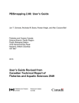
Figure 1. Map of the world ............................................................................................................. 6
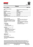
Figure 2. Map of the northeastern Pacific Ocean (longitude-latitude) ........................................... 7
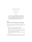
Figure 3. Map of the northeastern Pacific Ocean (UTM easting-northing).................................... 8
Figure 4. Illustration of the thinPolys function ...................................................................... 12
Figure 5. Example of the joinPolys logic operations ............................................................. 14
Figure 6. Several polylines in a continuous S-PLUS contour ...................................................... 16
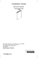
Figure 7. Tow tracks from a longspine thornyhead survey in 2001 ............................................. 17
Figure 8. Areas of islands in the southern Strait of Georgia......................................................... 18
Figure 9. Pacific ocean perch survey data (1966-89) ................................................................... 19
Figure 10. Proof of Pythagoras’ Theorem .................................................................................... 20
Figure D1. PBS Mapping compared with GMT – Vancouver Island........................................... 31
Figure D2. PBS Mapping compared with GMT – tow tracks ...................................................... 33
–v–
ABSTRACT
Schnute, J.T., Boers, N.M., and Haigh, R. 2004. PBS Mapping 2: user’s guide.
Can. Tech. Rep. Fish. Aquat. Sci. 2549: 126 + viii p.
This report describes a second version of software designed to facilitate the compilation
and analysis of fishery data, particularly data referenced by spatial coordinates. Our research
stems from experiences with information on Canada’s Pacific groundfish fisheries compiled at
the Pacific Biological Station (PBS). Despite its origins in fishery data analysis, our software has
broad applicability. The library PBS Mapping extends the languages R and S-PLUS to include
two-dimensional plotting features similar to those commonly available in a Geographic
Information System (GIS). Embedded C code speeds algorithms from computational geometry,
such as finding polygons that contain specified point events or converting between longitudelatitude and Universal Transverse Mercator (UTM) coordinates. We also present a number of
convenient utilities for Microsoft Windows operating systems that support computational
geometry outside the framework of R or S-PLUS. Our results, which depend significantly on the
work of students, illustrate the convergence of goals between academic training and applied
research.
RÉSUMÉ
Schnute, J.T., Boers, N.M. et Haigh, R. 2004. PBS Mapping 2 : Guide de l’utilisateur.
Can. Tech. Rep. Fish. Aquat. Sci. 2549: 126 + viii p.
Le présent rapport décrit la seconde version du logiciel conçu pour faciliter la
compilation et l’analyse de données halieutiques, en particulier les données référencées par des
coordonnées spatiales. Nos travaux de recherche ont capitalisé sur des expériences menées à
l’aide de données sur les pêches des poissons démersaux le long du littoral Pacifique du Canada,
données compilées à la Station biologique du Pacifique (SBP). Bien que conçu initialement pour
l’analyse de données halieutiques, notre logiciel peut s’appliquer à toute une variété de
domaines. La bibliothèque PBS Mapping (Cartographie de la SBP) étend le langage R et SPLUS pour inclure une capacité d’impression en deux dimensions semblable à celle
habituellement disponible dans les systèmes d’information géographiques (SIG). Des modules en
C permettent d’accélérer les algorithmes grâce à la géométrie numérique, en trouvant par
exemple les polygones qui contiennent des événements ponctuels spécifiques ou en convertissant
les longitudes et les latitudes en coordonnées de la projection transversale universelle (UTM).
Nous présentons également un certain nombre d’applications intéressantes pour les systèmes
d’exploitation Microsoft Windows, qui peuvent effectuer des opérations de géométrie numérique
en dehors du cadre de travail R et S-PLUS. Nos résultats, auxquels plusieurs étudiants ont
grandement contribué, illustrent la convergence des objectifs de la formation académique et de la
recherche appliquée.
– vi –
PREFACE
During the last decade, I’ve had the pleasure of directing work by computer science
students from various local universities. My research as a mathematician in fish stock assessment
requires an extensive software toolkit, including statistical languages, compilers, and operating
system utilities. It helps greatly to have bright, adaptive students who can learn new languages
quickly, investigate software possibilities, answer technical questions, and design programs that
assist scientific analysis. I’m particularly grateful for contributions from the following students:
• Robert Swan (University of Victoria), 1996;
• Mike Jensen (Malaspina University-College and Simon Fraser University), 1997 and 1999;
• Chris Grandin (Malaspina University-College), 2000 and 2001;
• Nick Henderson (Malaspina University-College), 2002;
• Nick Boers (Malaspina University-College), 2003 and 2004.
Starting in 1998, I began a formal connection with the Computing Science Department at
Malaspina University-College (MUC). My discussions with faculty members, particularly Dr.
Peter Walsh and Dr. Jim Uhl, highlighted the convergence of goals between academic training
and scientific research. Projects designed for fish stock assessment give students an opportunity
to further their computing science careers while producing useful software. Both MUC and the
Pacific Biological Station (PBS), where I work, are located in Nanaimo, British Columbia,
Canada. This happy juxtaposition makes it easy to engage students in the exchange of ideas
between academia and applied research. For example, Jim Uhl participated directly in Nick
Boers’ PBS work term during the summer of 2003. Nick had completed a course in computer
graphics taught by Jim in the fall of 2002. Algorithms in the textbook (Foley et al. 1996) proved
invaluable for writing software to produce maps of the British Columbia coast with related
fishery information.
Quantitative fishery science requires a strong connection between theory and practice. In
his book on computing theory, Michael Sipser (1997, p. xii) tells students that:
“. . . theory is good for you because studying it expands your mind. Computer
technology changes quickly. Specific technical knowledge, though useful today,
becomes outdated in just a few years. Consider instead the abilities to think, to express
yourself clearly and precisely, to solve problems, and to know when you haven't solved
a problem. These abilities have lasting value. Studying theory trains you in these areas.”
While dealing with the issues addressed here, I found myself asking simple questions that have
numerically interesting answers. How do you locate fishing events within management areas or
other polygons? How should regional boundaries on maps be clipped to lie within a smaller
rectangle? I soon realised that I had touched upon the emerging field of computational geometry,
where people have devised clever and efficient algorithms for addressing such questions.
Remarkably effective software can now be obtained freely from the Internet. I’m
particularly fond of R, a version of the powerful statistical language S (and later S-PLUS)
devised by Becker et al. (1988). Venables and Ripley (1999, 2000) give excellent guidance for
using either language. Although written originally for Unix, R has also been implemented for
– vii –
Microsoft’s Windows operating systems. The web site http://cran.r-project.org/ describes R as
GNU S, “a freely available language and environment for statistical computing and graphics”.
The GNU project (http://www.gnu.org/), where the recursive acronym GNU means “GNU’s Not
Unix”, offers a wealth of free software including compilers for C/C++, Fortran, and Pascal. Code
can be written in these compiled languages to speed computations that would otherwise run more
slowly in R/S. Nick Boers has used such linkages intelligently to bring fast computational
geometry into our package PBS Mapping, written for both R and S-PLUS.
To some extent, this report constitutes a second edition of an earlier report (Schnute et al.
2003) that describes a suite of software utilities developed at PBS. In particular, the package PBS
Mapping has undergone extensive renovations and improvements, and this document provides a
definitive manual for using version 2. To accommodate the new material presented here, my
co-authors and I have decided to remove sections of the earlier report that discuss other PBS
software utilities, free software available on the Internet, and related technical information.
Readers of this current report may also wish to acquire the earlier version for additional material
not included here.
I want to mention two milestones achieved during the production of PBS Mapping,
Version 2. First, we have posted the current software as a contributed package on the
Comprehensive R Archive Network (CRAN, http://cran.r-project.org/). Thanks to a remarkable
collection of Perl scripts developed for the R project, source code in both C and R, along with
suitable documentation files, can be tested and compiled automatically for distribution as both
source and binary packages. Nick Boers ensured that our source materials met the necessary
standards, and (after we made minor changes in the C code to avoid compiler warnings) the
authors of the CRAN web site in Vienna, Austria accepted our contribution. Second, Nick
applied to the Canadian Natural Sciences and Engineering Research Council (NSERC) for a
grant to support graduate studies in computing science. His application cited his successful
experience developing PBS Mapping, Version 1, as documented in Schnute et al. (2003). To the
delight of Nick’s supporters at PBS and MUC, he won a substantial award, in fact the only
NSERC grant given to a student from MUC this year. Congratulations, Nick, from your
colleagues at PBS and professors at MUC. We’ll follow your career at the University of Alberta
in Edmonton with great interest.
Jon Schnute
– viii –
This page has been left intentionally blank for printing purposes.
–1–
1. INTRODUCTION
This report describes software written to facilitate the compilation and analysis of fishery
data, particularly data referenced by spatial coordinates. Our work developed from experiences
constructing databases that capture information from Canada’s Pacific groundfish fisheries.
Fishing events take place across a broad range of coastal waters and result in the capture of many
species. Initially, we focused on issues related to database design and development, as described
in previous reports by Schnute et al. (1996), Haigh and Schnute (1999), Rutherford (1999),
Schnute et al. (2001, Section 2 and Appendix A), and Sinclair and Olsen (2002). Analyses of
these databases shifted our attention to the problem of portraying and understanding such
complex information. Maps with statistical information proved especially useful, and we found
ourselves facing questions commonly addressed by Geographic Information Systems (GIS).
Commercial GIS packages can be expensive, with an additional requirement for
specialised training. Because analysts who deal with Pacific groundfish data often have
experience using the statistical languages R (http://cran.r-project.org/, available for free) or
S-PLUS (http://www.insightful.com/, available commercially), we began by writing bilingual
functions for these languages to produce the maps required. Schnute et al. (2003) describe the
package PBS Mapping, Version 1, which evolved from these early experiences. After another
year of development, we have extensively revised the software, and this current report serves
primarily as a user’s manual for PBS Mapping, Version 2. The Preface explains the relationship
between this document and its predecessor (Schnute et al. 2003).
Section 2 covers the mapping software itself, which contains functions that perform
numerous calculations on polygons. These include standard set theoretic operations (union,
intersection, difference, exclusive-or), clipping, thinning, thickening, testing convexity, forming
the convex hull, and calculating various statistics (such as mean, centroid, and area). We discuss
public data that represent shorelines and ocean bathymetry, and the package includes sample data
sets drawn from these sources. We also discuss the Universal Transverse Mercator (UTM)
projection that gives a particularly accurate flat projection of the earth’s surface. Our software
can convert between longitude-latitude and UTM coordinates.
Section 3 documents a number of convenient command-line utilities, compiled separately
from C code written for the PBS Mapping package. These make it possible to perform some of
the polygon functions outside the framework of R or S. Appendices provide additional
information about various topics related to PBS Mapping, including
A. the contents of the distribution CD for this software;
B. an Internet source for global shoreline data;
C. an Internet source for global bathymetry data;
D. alternative Generic Mapping Tools (GMT);
E. source code for the figures in this report;
F. changes in PBS Mapping from Version 1 to Version 2;
G. function dependencies in PBS Mapping;
H. documentation for PBS Mapping functions and data;
I. a package of supplementary data for PBS Mapping, of interest to local users at PBS.
–2–
We anticipate that our software will continue to change for the better, due to bug fixes
and other improvements. This report documents version 2.00, which currently appears as a
contributed package on the R archive (http://cran.r-project.org/). We will post subsequent
versions as they become available. Our distribution CD, which may eventually be posted on the
Internet, includes the equivalent package for S-PLUS. A developer’s guide (Boers et al. 2004)
describes the process of building PBS Mapping from source materials for R and S and lists all
required software. Except for the commercial product S-PLUS, all software required to develop
and use PBS Mapping is freely available from the Internet.
1.1. Software Installation
Our distribution CD (Appendix A) includes two subdirectories \PBSmapping\ and
\PBSdata\ that provide everything necessary to install two packages:
• PBSmapping – the mapping software discussed in Section 1;
• PBSdata – various additional data sets relevant to fisheries investigated at PBS
(Appendix I).
Each package can be installed in three software environments: R (version 1.90 or higher),
S-PLUS 2000, and S-PLUS 6. In the discussion below, we describe the installation procedure for
PBSmapping, where a similar procedure applies to PBSdata. Our software appears in four
files:
• \PBSmapping\R\PBSmapping_2.00.tar.gz – source code for the R distribution,
which can be used to build a binary package;
• \PBSmapping\R\PBSmapping_2.00.zip – binary package ready for installation into
R;
• \PBSmapping\S-PLUS_2000\PBSmapping_2.00_Splus2000.zip – source
code and binary package ready for installation into S-PLUS 2000;
• \PBSmapping\S-PLUS_6\PBSmapping_2.00_Splus6.zip – source code and
binary package ready for installation into S-PLUS 6.
To install PBSmapping in R, start the R GUI. Click on the menu “Packages” and
choose the option “Install package(s) from local zip files…”. Find and select the file
PBSmapping_2.00.zip; then click on the button “Open”. Alternatively, it may also be
possible to choose the option “Install package(s) from CRAN…”, and then select PBSmapping.
To install PBSmapping in S-PLUS 2000, decompress the file
PBSmapping_2.00_Splus2000.zip into the S-PLUS library\ directory
(e.g., C:\Program Files\SP2000\library\). Make sure to invoke the option of using
complete folder names. This creates the subdirectory tree library\PBSmapping\. Similar
instructions apply to S-PLUS 6, using the file PBSmapping_2.00_Splus6.zip.
To remove PBSmapping from R or S-PLUS, open the library\ directory and delete
the associated subdirectory PBSmapping\. Before loading a new version of a package, we
recommend the removal of any previous version. Eventually, the installation files may have
names that reflect a version number later than the current version 2.00.
–3–
2. PBS MAPPING 2: FUNCTIONS AND DATA
Niklaus Wirth, the author of Pascal and Modula-2, summarises the essence of software
design in the title of his book Algorithms + Data Structures = Programs (Wirth 1975). Our
software package PBS Mapping begins with data structures that embody two essential concepts.
First, polygons define boundaries, such as shorelines and fishery management areas. Second,
fishing events occur at specific locations defined by two geographical coordinates, such as
longitude and latitude. The languages R and S conveniently support such structures through the
concept of a data frame, essentially a database table in which rows and columns define records
and fields, respectively. Objects like data frames in R/S can also have attributes that store
additional properties, such as the projection used in defining a geographic coordinate system.
2.1. Data Structures for Maps
PBS Mapping introduces four data structures, each stored as a data frame. Field names,
attributes, and other properties of these objects implicitly dictate their type. An object may also
identify its type explicitly in the class attribute. Each type requires a particular structure, as
outlined below.
PolySet
In our software, a PolySet data frame defines a collection of polygonal contours (i.e., line
segments joined at vertices), based on four or five numerical fields:
• PID – the primary identification number for a contour;
• SID – (optional) the secondary identification number for a contour;
• POS – the position number associated with a vertex;
• X
– the horizontal coordinate at a vertex;
• Y
– the vertical coordinate at a vertex.
The simplest PolySet lacks an SID column, and each PID corresponds to a different contour. By
analogy with a child’s “follow the dots” game, the POS field enumerates the vertices to be
connected by straight lines. Coordinates (X, Y) specify the location of each vertex. Thus, in
familiar mathematical notation, a contour consists of n points ( xi , yi ) with i = 1, K , n , where i
corresponds to the POS index. A PolySet has two potential interpretations. The first associates a
line segment with each successive pair of points from 1 to n, giving a polyline (in GIS
terminology) composed of the sequential segments. The second includes a final line segment
joining points n and 1, thus giving a polygon.
The secondary ID field allows us to define regions as composites of polygons. From this
point of view, each primary ID identifies a collection of polygons distinguished by secondary
IDs. For example, a single management area (PID) might consist of two fishing areas, each
associated with a different SID. A secondary polygon can also correspond to an inner boundary,
like the hole in a doughnut. We adopt the convention that POS goes from 1 to n along an outer
boundary, but from n to 1 along an inner boundary, regardless of rotational direction. This
contrasts with other GIS software, such as ArcView (ESRI 1996), in which outer and inner
boundaries correspond to clockwise and counter-clockwise directions, respectively.
–4–
The SID field in a PolySet with secondary IDs must have integer values that appear in
ascending order for a given PID. Furthermore, inner boundaries must follow the outer boundary
that encloses them. The POS field for each contour (PID, SID) must similarly appear as integers
in strictly increasing or decreasing order, for outer and inner boundaries respectively. If the POS
field erroneously contains floating-point numbers, fixPOS can renumber them as sequential
integers, thus simplifying the insertion of a new point, such as point 3.5 between points 3 and 4.
A PolySet can have a projection attribute, which may be missing, that specifies a
map projection. In the current version of PBS Mapping, projection can have character
values "LL" or "UTM", referring to “Longitude-Latitude” and “Universal Transverse Mercator”.
We explain these projections more completely below. If projection is numeric, it specifies
the aspect ratio r, the number of x units per y unit. Thus, r units of x on the graph occupy the
same distance as one unit of y. Another optional attribute zone specifies the UTM zone (if
projection="UTM") or the preferred zone for conversion from Longitude-Latitude (if
projection="LL").
A data frame’s class attribute by default contains the string "data.frame".
Inserting the string "PolySet" as the class vector’s first element alters the behaviour of
some functions. For example, the summary function will print details specific to a PolySet.
Also, when PBSprint is TRUE, the print function will display a PolySet’s summary rather
than the contents of the data frame.
PolyData
We define PolyData as a data frame with a first column named PID and (optionally) a
second column named SID. Unlike a PolySet, where each contour has many records
corresponding to the vertices, a PolyData object must have only one record for each PID or each
(PID, SID) combination. Conceptually, this object associates data with contours, where the data
correspond to additional fields in the data frame. The R/S language conveniently allows data
frames to contain fields of various atomic modes (“logical”, “numeric”, “complex”, “character”,
and “null”). For example, PolyData with the fields (PID, PName) might assign character names
to a set of primary polygons. Additionally, if fields X and Y exist (perhaps representing locations
for placing labels), consider adding attributes zone and projection. Inserting the string
"PolyData" as the class attribute’s first element alters the behaviour of some functions,
including print (if PBSprint is TRUE) and summary.
Our software particularly uses PolyData to set various plotting characteristics. Consistent
with graphical parameters used by the R/S functions lines and polygon, column names can
specify graphical properties:
• lty
– line type in drawing the border and/or shading lines;
• col
– line or fill colour;
• border
– border colour;
• density – density of shading lines;
–5–
• angle
– angle of shading lines.
When drawing polylines (as opposed to closed polygons), only lty and col have meaning.
EventData
We define EventData as a data frame with at least three fields named (EID, X, Y).
Conceptually, an EventData object describes events (EID) that take place at specific points
(X, Y) in two-dimensional space. Additional fields specify measurements associated with these
events. For example, in a fishery context EventData could describe fishing events associated
with trawl tows, based on the fields:
• EID
– fishing event (tow) identification number;
• X, Y
– fishing location;
• Duration – length of time for the tow;
• Depth
– average depth of the tow;
• Catch
– biomass captured.
Like PolyData, EventData can have attributes projection and zone, which may be absent.
Inserting the string "EventData" as the class attribute’s first element alters the behaviour
of some functions, including print (if PBSprint is TRUE) and summary.
LocationSet
A PolySet can define regional boundaries for drawing a map, and EventData can give
event points on the map. Which events occur in which regions? Our function findPolys,
discussed in Section 2.3 below, solves this problem. The output lies in a LocationSet, a data
frame with three or four columns (EID, PID, SID, Bdry), where SID may be missing. One row
in a LocationSet means that the event EID occurs in the polygon (PID, SID). The boundary
(Bdry) field specifies whether (Bdry=T) or not (Bdry=F) the event lies on the polygon
boundary. If SID refers to an inner polygon boundary, then EID occurs in (PID, SID) only if
Bdry=T. An event may occur in multiple polygons. Thus, the same EID can occur in multiple
records. If an EID does not fall in any (PID, SID), or if it falls within a hole, it does not occur in
the output LocationSet. Inserting the string "LocationSet" as the first element of a
LocationSet’s class attribute alters the behaviour of some functions, including print (if
PBSprint is TRUE) and summary.
2.2. Map Projections
The simplest projection associates each point on the earth’s surface with a longitude
x ( − 360° ≤ x ≤ 360° ) and latitude y ( − 90° ≤ y ≤ 90° ), where x = 0° on the Greenwich prime
meridian. The chosen range of x depends on the region of interest, where negative longitudes
refer to displacements west of the prime meridian. When plotted on a rectangular grid with equal
distances for each degree of longitude and latitude, this projection exaggerates the size of objects
near the earth’s poles, as illustrated in Figure 1. For points near the latitude y, a more realistic
map uses the aspect ratio
–6–
r=
(2.1)
1
,
cos y
where r degrees of longitude x should occupy the same distance as 1 degree of latitude y.
-50
Latitude (°)
0
50
123456789
0
100
200
Longitude (°)
300
Figure 1. Map of the world projected in longitude-latitude coordinates. This image, based on our
PolySet worldLL, uses the longitude range − 20° ≤ x ≤ 360° to produce a convenient cut in the
eastern Atlantic Ocean. Red vertical lines show boundaries for the 60 Universal Transverse
Mercator (UTM) zones, with explicit labels for zones 1 to 9. A black line indicates the prime
meridian ( x = 0°) . Our PolySet nepacLL lies within the clipping boundary shown as a blue
rectangle.
The Universal Transverse Mercator (UTM) projection gives a more realistic portrayal of
the earth’s surface within 60 standardized longitude zones. Each zone spans 6° , and zone i
includes points with longitude x in the range
(2.2)
(−186 + 6i )° < x ≤ (−180 + 6i )°
[UTM zone i]
The mid-longitude in (2.2)
(2.3)
xi = ( −183 + 6i )°
[Central meridian, zone i]
defines the central meridian of zone i. In particular, zone 9 has central meridian − 129° and
covers the range
(2.3)
− 132° < x ≤ −126° .
[UTM zone 9]
Canada’s Pacific coast lies in zones 8 to 10 (Figure 2), and the projection to zone 9 gives a
reasonably accurate map for fisheries in this region.
60 1
2
3
4
5
6
7
8
9 10 11
40
Latitude (°)
50
60
70
–7–
-180
-160
-140
-120
Longitude (°)
Figure 2. Shoreline data in longitude-latitude coordinates for the northeastern Pacific Ocean, as
captured in our PolySet nepacLL. Vertical red lines display UTM boundaries for zones
60, 1, 2, …, 11. A vertical dotted line indicates the central meridian of zone 6, near the centre of
this figure.
Visually, UTM zones look like sections of orange peel cut from top to bottom. Each
relatively narrow section can be flattened without too much distortion to give coordinates ( X , Y )
measured as actual distances, as illustrated by zone 6 in Figure 3. Complex formulas, compiled
in detail by the UK Ordnance Survey (Anonymous 1998), allow conversion between two
projections: the UTM easting-northing coordinates ( X , Y ) and the usual longitude-latitude
coordinates ( x, y ) . These take account of the earth’s ellipsoidal shape, with a wider diameter at
the equator than the poles. The UTM projection scales distances exactly along two great circles:
the equator and the central meridian, which act as X and Y axes, respectively. Along the
equator, Y = 0 km by definition; elsewhere, Y indicates the distance north (positive Y) or south
(negative Y) of the equator. The central meridian is assigned a standard easting X = 500 km,
rather than the usual X = 0 km. This ensures that X > 0 km throughout the zone. In effect, the
difference X − 500 km represents the distance east of the central meridian, where a negative
distance corresponds to a westward displacement. These interpretations are exact along the
equator and central meridian, but approximate elsewhere.
60
1
2
3
4
5
6
7
8
9 10
11
5000
UTM Northing (km)
6000
7000
8000
–8–
-2000
-1000
0
1000
UTM Easting (km)
2000
3000
Figure 3. Shoreline data for the northeastern Pacific Ocean, projected in UTM coordinates
(zone 6) from our PolySet nepacLL. Vertical red lines show UTM zone boundaries. The central
axis of zone 6 (vertical dotted line at x = 500 km) corresponds to the central meridian shown in
Figure 2.
2.3. PBS Mapping Functions and Algorithms
Our software produces maps from the data structures defined in Section 2.1. Following
typical design concepts in R/S, it uses functions to generate plots, implement algorithms, and
perform other tasks. Where possible, function arguments often have explicit default values.
PBS Mapping includes many functions not mentioned in this section. We encourage readers to
examine Appendix H, which gives detailed technical descriptions of all our software’s functions
and other components. Table H1 provides a concise summary for easy reference.
Graphics Functions
In the R/S language, high-level commands (like plot) create new graphs; lower-level
commands (like points and lines) add features to an existing graph. Similarly, we provide
functions (plotLines, plotMap, plotPoints, plotPolys) that create graphs and others
(addLabels, addLines, addPoints, addPolys, addStipples) that add graphical
features.
–9–
Some of these plotting functions draw objects defined by a PolySet, while others expect
EventData, a LocationSet, or PolyData. Both plotLines and addLines treat their input
PolySet as polylines, with no connection between the last and first vertices. By contrast,
plotMap, plotPolys, and addPolys regard their input as polygons, where a final line
segment connects the last vertex to the first. The functions plotMap and plotPolys behave
similarly, except that plotMap’s default behaviour guarantees the correct aspect ratio, as
defined by either the PolySet’s projection attribute or the function’s projection
argument. If both are specified, the attribute supersedes the argument. When this attribute is
missing, plotMap uses a 1:1 projection. Table 1 summarises the default behaviour of our
principal graphics commands. A user concerned with drawing maps, where the correct aspect
ratio plays a key role, would likely initiate a graph with the plotMap function. However,
plotPolys, plotLines, and plotPoints can also set the correct aspect ratio when
passed a suitable projection argument.
Table 1. Behaviour of the principal graphics functions in the PBS Mapping software package.
Function
Creates a Graph
addLabels
addLines
addPoints
addPolys
addStipples
plotLines
plotMap
plotPoints
plotPolys
No
No
No
No
No
Yes
Yes
Yes
Yes
Plots as Polygons Sets Aspect Ratio
by Default
No
Yes
No
No
Yes
Yes
No
Yes
No
Our high-level graphics functions accept a common set of arguments, consistent with
existing par parameters where possible. These include
• xlim and ylim to specify horizontal and vertical coordinate ranges;
• projection to specify the projection used in drawing the map or graph;
• plt to define the plot region relative to the figure region;
• polyProps to support plotting properties for individual contours (Section 2.1);
• lty, cex, col, border, density, pch, and angle to adjust properties of labels, lines,
points, and polygons where applicable;
• axes to disable plotting axes;
• tck to control (major) tick mark lengths;
• tckMinor, a counterpart of tck, to set a different length for minor tick marks;
• tckLab, with Boolean values, to determine whether to include numeric tick labels.
We introduce tckMinor and tckLab to give finer control over the appearance of tick marks.
Each of tck, tckLab, and tckMinor can have length one or two. A single value pertains to
– 10 –
both axes, and two values specify distinct parameters for the horizontal and vertical axes,
respectively.
Our low-level graphics functions (e.g., addLines) use many of the same arguments as
their high-level counterparts (e.g., plotLines). However, they do not accept parameters that
affect the overall plot, such as xlim, ylim, projection, plt, axes, or any of the tck
arguments.
The par parameter plt plays a special role in PBS Mapping, because we use it to set
the aspect ratio required for a particular projection. Recall that in R/S the plot region lies
inside the figure region, which similarly lies inside the overall device region. The parameter plt
specifies the plot region boundaries as fractions (left, right, bottom, top) of the current figure
region. Our high-level plotting functions use the initial default value
plt=c(0.11,0.98,0.12,0.88),
but then alter plt by shrinking the width or height to achieve the required aspect ratio. In the
function call, the argument plt can set a different default value, but again this may be changed
by the graphics function to set the aspect ratio. In effect, the argument plt sets minimum
margins for the plot within the figure region, but the aspect ratio may force the plot to shrink in
width or height, giving wider margins in one direction.
Standard high-level commands in R/S (like plot) do not allow layout parameters (like
plt) to be passed as arguments. Instead, users normally use par to set these parameters before
invoking a graphics command. However, unlike normal graphics commands, those in PBS
Mapping actually alter the margins, so we adopt a different approach in which plt is reset with
each high-level command. Advanced users wishing to set the plot region using the par
parameters mai or mar can disable the default initial size with the argument plt=NULL.
Computational Functions
PBS Mapping contains many functions that perform computations on PolySets and other
data structures. Appendix H lists them all, but we give further details for some of them here,
including formulas or algorithms for implementation and references for further reading. In
alphabetic order, this list below highlights key features of selected functions in the package.
• calcArea computes polygon areas by the formula (Rokne 1996)
A=
•
1
2
n −1
∑ (x y
i =1
i
i +1
− xi +1 yi ) ,
for the area A of a polygon with vertices ( xi , yi ), i = 1, K , n , where vertices 1 and n
correspond to the same point: ( x1 , y1 ) = ( xn , y n ) . This formula assumes identical units for x
and y (an aspect ratio 1), as in UTM coordinates. The function automatically converts
longitude-latitude coordinates to UTM before calculating the area.
calcCentroid computes polygon centroid coordinates ( x, y ) by the formulas
(Bourke 1988)
– 11 –
1 n −1
x=
∑ (xi + xi+1 )(xi yi+1 − xi+1 yi )
6 A i =1
1 n −1
y=
∑ ( yi + yi+1 )(xi yi +1 − xi+1 yi )
6 A i =1
•
•
for a polygon with vertices ( xi , yi ), i = 1, K , n , where vertices 1 and n correspond to the
same point: ( x1 , y1 ) = ( xn , y n ) and A is computed by the formula shown above in the
definition of calcArea. These formulas scale automatically to the units of x and y and
consequently do not depend on the projection attribute.
calcConvexHull calculates the convex hull for a given set of points using an algorithm
presented by de Berg et al. (2000, the “incremental algorithm” on p. 6-7).
calcLength calculates polyline lengths using Pythagoras’ Theorem when the projection is
UTM or 1. Thus, the distance d between points ( x, y ) and ( x ' , y ' ) is
d = ( x '− x ) 2 + ( y '− y ) 2 .
The function also supports longitude-latitude coordinates ( x, y ) by calculating great circle
distances between polygon vertices. In this case, the distance d between two points is
(Chamberlain 2001)
⎡
⎤
⎛ y '− y ⎞
2 ⎛ x '− x ⎞
d = 2 R arcsin ⎢ sin 2 ⎜
⎟ + (cos y ) (cos y ' ) sin ⎜
⎟⎥ ,
⎝ 2 ⎠ ⎥⎦
⎝ 2 ⎠
⎢⎣
•
•
•
•
•
•
•
•
•
•
•
where R = 6371.3 km denotes the earth’s mean radius (Wikipedia 2004).
calcMidRange calculates midpoints of the X and Y ranges for each given polygon.
calcSummary calculates summary statistics for a PolySet, given a user-defined function.
clipLines (and clipPolys) clips polylines (and polygons) within a specified
rectangle, possibly smaller than the bounding rectangle, using the Sutherland-Hodgman
clipping algorithm (Foley et al. 1996, p. 124-127).
closePolys adds corners from the bounding rectangle, if needed, to close polylines into
polygons.
convUL converts between UTM and longitude-latitude coordinates using the extensive
formulas presented in Anonymous (1998).
findPolys finds the polygons in a PolySet that contain events specified in EventData,
using the “crossings test” algorithm described later in this section.
isConvex determines which polygons in a PolySet are convex, using an algorithm
described below.
isIntersecting finds polygons that self-intersect by comparing each edge pairwise with
every other edge.
joinPolys performs set theoretic operations (union, intersection, difference, and
exclusive-or) on polygons using the General Polygon Clipper (GPC) library by Murta (2004).
thickenPolys adds vertices to polygons using an algorithm described below.
thinPolys thins the number of polygon vertices, based on the Douglas-Peuker line
simplification algorithm (Douglas and Peucker 1973), as illustrated in Figure 4.
Latitude (°)
48.5 49 49.5 50 50.5 51
– 12 –
A
-128
-127 -126 -125
Longitude (°)
-124
B
-128
-127 -126 -125
Longitude (°)
-124
Figure 4. (A) Vancouver Island clipped from the PolySet nepacLL and (B) the result of
applying thinPolys to this polygon with a tolerance of ten kilometres.
Our function isConvex first calls isIntersecting to determine whether or not a
polygon self-intersects. If it does, it cannot be convex and the result is FALSE. Otherwise, the
function proceeds. Three sequential points in a non-self-intersecting polygon describe a left turn,
a straight line, or a right turn. The function locates the first non-straight turn (left or right) in a
polygon and checks that all subsequent turns are either the same or straight. If so, the polygon is
convex; otherwise it is not.
Like calcLength, thickenPolys also supports the longitude-latitude projection. In
this case, tol is measured in kilometres and distances are computed along great circles
(Chamberlain 2001).
When the projection is UTM or 1, our function thickenPolys accepts a tolerance
specified in X or Y units (kilometres in the UTM case). It operates in two distinct modes. When
keepOrig=TRUE, it retains all original vertices and adds vertices, as required, along each edge.
Thus, if the distance between two sequential original vertices exceeds the specified tolerance
tol, it adds enough vertices spaced evenly between them so that sequential vertices lie at most
the distance tol apart. When keepOrig=FALSE, the algorithm guarantees only that the first
vertex of each polygon appears in the result. Starting at that vertex, the algorithm walks through
the polygon while summing distances between vertices. When the cumulative distance exceeds
tol, it adds a vertex on the line segment under inspection. It then resets the distance sum and
continues walking the polygon from this new vertex.
Associating Points with Polygons
As discussed in the definition of LocationSet (Section 2.1), our function findPolys
solves the “points-in-polygons” problem. Given a set of points (EventData) and a collection of
polygons (a PolySet), which points lie in which polygons? Several algorithms solve this
problem, including:
– 13 –
•
The angle summation (or winding number) test. Sum the angles swept by a ray from the
trial point to sequential vertices of the polygon. For a point outside the polygon, the angles
sum to 0 because the ray sweeps back and forth, returning to the starting point. For an inside
point, the ray traces a full circle, and the angles do not sum to zero.
• The crossings test. Draw a ray from the trial point in a fixed direction (e.g., upward). If the
ray crosses an even number of polygon edges, the point must be outside. For an inside point,
the number of crossings must be odd.
We use the crossings test because it performs faster than angle summation (Hains 1994, p. 2627). The latter requires large numbers of trigonometric function calls.
After finding the polygons that contain various events, an analyst often wants to compute
statistics associated with the events that occur inside each polygon. For example, in a fishery
context, what is the total catch from all fishing events within each management region? Our
function combineEvents supports such calculations. The function makeProps can then
relate polygon properties, such as colour used for plotting, to these computed statistical values.
Set Theoretic Operations
We include the function joinPolys to apply set theoretic operations (difference,
intersection, union, and exclusive-or) to one or two PolySets. Our joinPolys function
interfaces with the General Polygon Clipper (GPC) library developed by Alan Murta (2004) at
the University of Manchester. We adopt some of his terminology in the discussion here. He
defines a generic polygon (or polygon set) as zero or more disjoint polygonal contours that
define boundaries of the polygon region. Some contours can represent inner boundaries that
define holes in the region. Each contour can be convex, concave, or self-intersecting.
In our PolySet, the polygons associated with each unique PID correspond to a generic
polygon with some restrictions. Some of our functions do not support self-intersecting polygons.
Furthermore, the SID contours cannot be arranged in arbitrary order because we require that
hole contours follow the outer contours in which they lie.
The function joinPolys can also accept two PolySet arguments P and Q. In this case,
the function returns a PolySet with all possible pairwise applications of op between generic
polygons in P and Q. For example, if P contains (A, B, C) and Q contains (D, E), then
joinPolys returns a PolySet with six PIDs corresponding to the six generic polygons A op D,
B op D, C op D, A op E, B op E, and C op E. More generally, if P and Q include m and n generic
polygons, respectively, then the function returns a PolySet with m × n generic polygons.
If m = 1 or n = 1 , the output preserves PIDs from the PolySet with more than one generic
polygon. Figure 5 illustrates the four supported set theoretic operations applied to crescentshaped polygons A and B.
Applied to one PolySet P, our function joinPolys applies the set theoretic operation
op sequentially to the generic polygons in P. For example, suppose that P contains three generic
polygons (A, B, C). Then the function returns a PolySet containing the generic polygon
((A op B) op C), represented as one PID with possibly many SIDs.
– 14 –
Figure 5. Example of the joinPolys logic operations. Panels A and B display the first and
second PolySets, respectively. Panels C to F illustrate the intersection, union, difference, and
exclusive-or operations, respectively.
2.4. Shoreline Data
To portray fishery data along Canada’s Pacific coast, we need a PolySet that defines the
relevant shoreline. We began with a polyline of the British Columbia coast, digitised manually
from a marine map. To convert this object to a meaningful closed polygon, we devised the
functions fixBound and closePolys. Satellite imagery and other sources, however, make
our initial coastline obsolete. For example, Wessel and Smith (1996) have used information from
the public domain to assemble a Global Self-consistent, Hierarchical, High-resolution Shoreline
(GSHHS) database for the entire planet. They make this available via the Internet as binary files
in five different resolutions: full, high, intermediate, low, and crude. They also supply software
as C source code for
• converting the data to an ASCII (plain text) format (gshhs.c);
• thinning the data by reducing the number of points sensibly (gshhs_dp.c).
– 15 –
Their thinning software uses an algorithm devised by Douglas and Peucker (1973), whose initials
dp appear in the file name. The dp is also an abbreviation of decimate polygons. We compiled
both programs with a free GNU compiler, as described in Appendix B.
Table 2. PolySets derived from the full resolution GSHHS database.
PolySet
nepacLL*
nepacLLhigh
worldLL*
worldLLhigh*
*
Thinning
0.2 km
0.1 km
5.0 km
1.0 km
Longitude
− 190° ≤ x ≤ −110°
− 190° ≤ x ≤ −110°
− 20° ≤ x ≤ 360°
− 20° ≤ x ≤ 360°
Latitude
34° ≤ y ≤ 72°
34° ≤ y ≤ 72°
− 90° ≤ y ≤ 84°
− 90° ≤ y ≤ 84°
Vertices
75,929
199,914
30,797
191,268
Polygons
536
9,961
210
1,502
Excludes polygons with fewer than 15 vertices after thinning.
PBS Mapping includes four data sets derived from the full resolution GSHHS database
(Table 2). These all use longitude-latitude (LL) coordinates. The nepac data sets contain the
northeastern Pacific Ocean shoreline in a region that extends roughly from California to Alaska
(Figure 2), and the world data sets cover the planet (Figure 1). As discussed in section 2.2,
longitude coordinates x take continuous values meaningful for the intended map, with x = 0° on
the Greenwich prime meridian.
We generated each data set from the full-resolution GSHHS database by following a
consistent sequence:
• thin the database with a specified distance tolerance, as listed in the above table, using
GSHHS software;
• convert the result to an ASCII file with GSHHS software;
• use our own Perl script (gshhs2r.pl) on this file to:
- remove the lakes, islands in lakes, and ponds in islands;
- eliminate small polygons, if desired, such as those with fewer than 15 vertices;
- transform this file to another ASCII file with the structure of a PolySet;
• clip the data to the desired coordinate range with our own stand-alone program
clipPolys.exe;
• import the ASCII table to a data frame in R/S;
• extend the Antarctic polygon data to longitude − 20° and latitude − 90° with the hidden
function .fixGSHHSWorld (world data sets only).
2.5. Bathymetry Data
Smith and Sandwell (1997) have produced global seafloor topography from satellite
altimetry and ship depth soundings. Their database appears on the Internet at
http://topex.ucsd.edu/cgi-bin/get_data.cgi. A web-based data acquisition form allows users to
extract a region after entering longitude and latitude coordinate ranges. Appendix C documents
how to import their data for use with PBS Mapping.
– 16 –
A
B
50.5
51
Latitude (°)
51.5
52
52.5
53
R and S-PLUS each provide a contour function to plot contour lines. The two
languages, however, implement this function differently, as itemized below.
• In S-PLUS, contour returns a list with coordinates of the contour lines when the save
argument is TRUE. Unfortunately, this list sometimes represents each continuous contour
with several polylines, as illustrated in Figure 6A.
• In R, contour lacks a save argument and does not return contour coordinates. Instead, the
contourLines function accomplishes this task, giving a list with somewhat different
format than the list produced by the S-PLUS contour function with the save=TRUE. The
R algorithm appears better than the one used by S-PLUS, because it tends to capture
continuous contours as single polylines (Figure 6B).
-131
-130
Longitude (°)
-129
-131
-130
Longitude (°)
-129
Figure 6. (A) The S-PLUS contour function with save=TRUE often returns several polylines
for a single continuous contour, illustrated here by cycling colours through SIDs. (B). The R
contourLines function returns a single polyline for each continuous contour.
In the S-PLUS version of PBS Mapping, we provide a contourLines function to
mimic the native R contourLines function; however, our software does not solve the
S-PLUS problem of several polylines for a continuous contour. In both R and S-PLUS, our
function convCP converts the list output from contourLines into a list object that has two
components: a PolySet with contour coordinates and PolyData with the depth of each contour.
The PBS Data package includes a data set (isobaths) of bathymetric contours for Canada’s
Pacific coast. In addition, several functions ease the manual procedure of converting polylines
into polygons, including
• convLP to convert two polylines into a single polygon;
– 17 –
•
•
closePolys to close the polygons in a PolySet;
fixBound to fix the boundary points of a PolySet.
2.6. Examples and Applications
Our library includes an illustrative PolySet towTracks containing the longitudelatitude coordinates of 45 tow tracks from a longspine thornyhead (Sebastolobus altivelis) survey
in 2001. Figure 7 portrays these data relative to the west coast of Vancouver Island, drawn with
shoreline data clipped from the PolySet nepacLL. The PolyData object towData specifies the
depth of each tow, represented in the figure by colours corresponding to depth intervals (black =
500-800 m, red = 800-1200 m, dark blue = 1200-1600 m).
48.5
Latitude (°)
49
49.5
Vancouver
Island
LTS Survey Tracks
500-800 m
800-1200 m
1200-1600 m
-127.5
-127
-126.5
Longitude (°)
-126
Figure 7. Tracks for 45 tows performed during the 2001 longspine thornyhead (Sebastolobus
altivelis) survey along the west coast of Vancouver Island (Starr et al. 2002). Each tow track is
colour-coded by depth stratum. Data come from the PolySet towTracks and PolyData
towData.
Figure 8 illustrates the use of our software to calculate polygon areas. We examine a
region along the south-west British Columbia coast that includes a cluster of islands in the Strait
of Georgia. Shoreline data come from the PolySet nepacLLhigh. Because area calculations do
not make sense in the longitude-latitude projection, we convert the PolySet to UTM coordinates,
with comparable X and Y coordinates (km), and then clip to the desired region. The figure shows
– 18 –
5440
areas for six selected islands, highlighted in yellow, based on the calcArea function. Island
centroids, derived using calcCentroid, give reference coordinates for printing island names
and areas.
Galiano
63
5430
Strait of Georgia
Saltspring
193
N Pender Saturna
35
30
5400
UTM Northing (km)
5410
5420
Mayne
26
5390
San Juan
149
5380
Vancouver Island
900
910
920
UTM Easting (km)
930
940
Figure 8. Areas (km2) of selected islands in the southern Strait of Georgia. Shoreline data have
been clipped from nepacLLhigh after conversion to UTM coordinates.
Figure 9 portrays data from Pacific ocean perch (Sebastes alutus) surveys conducted
along the central BC coast during the years 1966-1989. The EventData object surveyData
contains information from each tow, including the longitude, latitude, depth, catch, and effort
(tow duration). These data also imply the computed value of catch per unit effort
(CPUE = catch/effort). Code for this figure includes the following key function calls:
• plotMap to draw a coastal map of this region, clipped from nepacLL;
• makeGrid to create a grid in the region of interest;
• findPolys to associate tows with the appropriate grid cells;
• combineEvents to calculate the mean CPUE within each cell;
• addPolys to draw cells with colours (in the polyProps argument) scaled to the CPUE;
• points (the native R/S function) to plot events on the map.
POP Surveys (1966-89)
Latitude (°)
51.5
52
52.5
– 19 –
51
CPUE (kg/h)
0 - 50
50 - 300
300 - 750
750 - 1500
1500 - 25000
-131
-130
-129
-128
Longitude (°)
Figure 9. Portrayal of surveyData from Pacific ocean perch (Sebastes alutus) surveys in the
central coast region of British Columbia from 1966-89, with shoreline data clipped from
nepacLL. Colours portray the mean catch per unit effort (CPUE) within each grid cell
(0.1º by 0.1º). Circles show locations of individual tows.
PBS Mapping can also display non-geographical data, such as technical drawings,
network diagrams, and transportation schematics. For example, we use a PolySet to construct the
proof of Pythagoras’ Theorem in Figure 10, where the caption explains the logic leading to the
famous result a 2 + b 2 = c 2 . Incidentally, Devlin (1998, chapter 6, p. 221) mentions an historical
incident that nicely distinguishes maps from network diagrams. A now familiar drawing of the
London Underground (see the file “underground.pdf” at the web site
http://www.europrail.net/maps/) fails to represent geography correctly, but contains exactly the
information passengers need to navigate the system. It took two years for the designer, Henry C.
Beck, to persuade his superiors that his drawing would prove useful to the public.
– 20 –
Pythagoras' Theorem: a² + b² = c²
c
c²
b²
b
a²
a
Proof:
(a + b)² = 4 triangles + a² + b² = 4 triangles + c²
Figure 10. Proof of Pythagoras’ Theorem. A PolySet defines all geometric objects in this figure,
and PolyData determine the colours for plotting. Four blue triangles plus the yellow square ( a 2 )
and the green square (b 2 ) equal four blue triangles plus the red square ( c 2 ) ;
consequently, a 2 + b 2 = c 2 .
2.7. Strengths, Limitations, and Alternatives
PBS Mapping works with data exported from database tables, where records may not
have a definite order. The POS field in our PolySet definition imposes the required order for
polylines and polygons. This field also provides a convenient means of distinguishing inner and
outer boundaries. Our PolySets have a flat structure with at most two levels, corresponding to
primary and secondary IDs. We have found these limitations acceptable in the context of our
work. Sceptical readers might challenge our choices and prefer more complex hierarchical
structures. For example, Becker and Wilks (1993, 1995) define polygons as composites of
polylines, so that a common boundary between two regions need be defined only once and then
referenced in each regional definition. In our approach, all vertices of a common boundary must
be repeated in each regional definition.
– 21 –
We designed our software explicitly to address a few key issues in the spatial
representation of fishery data:
• easy importation from databases, Geographic Information Systems, and other sources, such
as the shoreline data compiled by Wessel and Smith (1996);
• precise control over the boundaries chosen for clipping from a larger map;
• support for longitude-latitude and UTM easting-northing coordinates;
• computational ability to associate events with polygons in which they lie;
• flexible plotting tools that summarise events within grids and other polygons.
Different purposes could well lead to other designs.
In addition to their comprehensive shoreline database, Wessel and Smith have designed
and released a free collection of Generic Mapping Tools (GMT; http://gmt.soest.hawaii.edu/)
that provide a serious alternative to our software. These tools operate in the DOS/UNIX
environment and support many more projections than PBS Mapping. They also store polygons in
a more efficient file format than our PolySet data frames. We designed PBS Mapping for the R/S
environment, with its rich support for statistical and mathematical analysis. We have also
included numerous algorithms from computational geometry, such as findPolys and
joinPolys. Readers may, however, find GMT more useful for map formats not supported in
PBS Mapping. Appendix D shows some comparative examples of code written in both
environments.
Because PBS Mapping includes features often supported by a Geographic Information
System (GIS), a free GIS package might also provide an alternative to the software described
here. The FreeGIS web site (http://www.freegis.org) summarises the current status of free GIS
programs and data. Their listings receive frequent updates and show a pattern of steady growth.
3. COMMAND-LINE UTILITIES
The PBS Mapping package for R/S includes several algorithms that we have also
implemented as stand-alone command-line utilities. These can handle very large data sets that
may be too large for the R/S working environment. Furthermore, some users may wish to
implement computational geometry calculations without reference to the R/S language. Our
utilities make this possible by directly processing text files with the appropriate data format.
They have been compiled with the same C code used for the dynamically linked library (DLL) in
R/S. For each utility, a corresponding .c file provides a front end to shared code for the
algorithms. Executable programs appear on our distribution CD in the directory
\CommandLineUtilities\.
3.1. clipPolys.exe (Clip Polygons)
The application clipPolys.exe reads an ASCII file containing a PolySet (explained
further below) and then clips it. The command
clipPolys.exe /i IFILE [/o OFILE] [/x MIN_X] [/X MAX_X] [/y MIN_Y]
[/Y MAX_Y]
– 22 –
has five arguments as follows:
ASCII input file containing a PolySet (required);
• /i IFILE
• /o OFILE
ASCII output file (defaults to standard output);
• /x MIN_X
lower X limit (defaults to minimum X in the PolySet);
• /X MAX_X
upper X limit (defaults to maximum X in the PolySet);
• /y MIN_Y
lower Y limit (defaults to minimum Y in the PolySet);
• /Y MAX_Y
upper Y limit (defaults to maximum Y in the PolySet).
The first line of the PolySet input file must contain the field names (PID, SID, POS, X, Y),
where SID is optional. Subsequent lines must contain the data, with the same number of fields
per row as in the header line. All fields must be delimited by white space. The program generates
a properly formatted PolySet. By default (unless otherwise specified by /o), this result goes to
standard output, which can be redirected to a text file (e.g., > file.txt).
3.2. convUL.exe (Convert between UTM and LL)
The application convUL.exe reads an ASCII file containing two fields named X and Y,
as described further below. The command
convUL.exe /i IFILE [/o OFILE] (/u | /l) /z ZONE
has the arguments:
ASCII input file containing the X and Y data (required);
• /i IFILE
• /o OFILE
ASCII output file (defaults to standard output);
• /u (or /l)
convert to UTM (longitude-latitude) coordinates (required);
• /z ZONE
source or destination zone for the UTM coordinates (required).
The input file must have an initial header line with field names, including X and Y. Subsequent
lines contain the data, with all fields separated by white space. The program converts each (X, Y)
pair to a new pair (X2, Y2). The output file matches the input file, with the fields (X2, Y2)
appended to the end of each line. The default standard output can be redirected to a text file.
3.3. findPolys.exe (Points-in-Polygons)
The application findPolys.exe reads two ASCII files: one containing a PolySet and
the other containing EventData. The program then determines which events fall inside the
available polygons. The command
findPolys.exe /p POLY_FILE /e EVENT_FILE [/o OFILE]
has the arguments:
• /p POLY_FILE
• /e EVENT_FILE
• /o OFILE
ASCII input file containing the PolySet (required);
ASCII input file containing EventData (required);
ASCII output file (defaults to standard output).
– 23 –
The header line in both input files must contain field names, and subsequent lines must contain
the relevant fields of data delimited by white space. The PolySet must have field names
(PID, SID, POS, X, Y), where SID is optional. The EventData must have fields (EID, X, Y).
The program writes a properly formatted LocationSet with three or four columns
(EID, PID, SID, Bdry), where SID may be missing (Section 2.1). The default standard output
can be redirected to a text file.
3.4. gshhs2r.pl (Convert GSHHS Data to PBS Mapping Format)
As discussed earlier in Section 2.4, our Perl script gshhs2r.pl converts data from the
Global Self-consistent, Hierarchical, High-resolution Shoreline (GSHHS) database to a PolySet
for use with PBS Mapping. We first require an ASCII file created by gshhs.exe, the program
supplied by the GSHHS project to convert binary to ASCII data. (Binary data may have been
thinned with gshhs_dp.exe.) Our utility removes non-ocean shorelines, such as lakes and
islands within lakes, as well as small polygons with N vertices or fewer. The command
gshhs2r.pl /i IFILE [/o OFILE] [/n N]
has arguments:
ASCII input file created by gshhs.exe (required);
• /i IFILE
• /o OFILE
ASCII output file for a PolySet (defaults to standard output);
• /n N
minimum number of vertices for an output polygon.
If the /n parameter is not specified, no filtering on the number of vertices takes place.
ACKNOWLEDGEMENTS
We thank Dr. Jim Uhl and Dr. Peter Walsh in the Computing Science Department,
Malaspina University-College, for encouraging and facilitating the role of students in applied
fisheries research. Without the dedicated work of these students, named in the Preface, we could
not have produced the software described here. We also acknowledge the valuable shoreline and
bathymetry databases compiled by Dr. Paul Wessel, Dr. Walter Smith, and Dr. D. T. Sandwell
(Wessel and Smith 1996; Smith and Sandwell 1997). In particular, we thank Dr. Paul Wessel for
permission to redistribute data from the GSHHS database. Code from other authors seriously
enhances this version of PBS Mapping. Dr. Alan Murta (through Toby Howard) has generously
given us permission to use his General Polygon Clipper (GPC) library, implemented in our
joinPolys function. Similarly, Dr. Gary Robinson has kindly allowed us to use his code for a
stack-based Douglas-Peuker line simplification routine, implemented in our thinPolys
function. Our colleague Brian Krishka helped prepare various data objects. The PBS Mapping
package could not exist without R and GCC. We express admiration and gratitude to the
remarkable teams that build, document, and distribute such outstanding free software.
– 24 –
REFERENCES
Anonymous. 1998. The ellipsoid and the Transverse Mercator projection. Geodetic Information
Paper No. 1 (version 2.2). Ordnance Survey, Southampton, UK. 20 p.
URL: http://www.ordsvy.gov.uk/.
Becker, R.A., Chambers, J.M., and Wilks, A.R. 1988. The new S language: a programming
environment for data analysis and graphics. Wadsworth and Books/Cole. Pacific Grove,
CA.
Becker, R.A., and Wilks, A.R. 1993. Maps in S. Statistics Research Report 93.2. AT&T Bell
Laboratories, Murray Hill, NJ. 21 p. URL: http://www.research.att.com/areas/stat/doc/.
Becker, R.A., and Wilks, A.R. 1995 (rev. 1997). Constructing a geographical database. Statistics
Research Report 95.2. AT&T Bell Laboratories, Murray Hill, NJ. 23 p.
URL: http://www.research.att.com/areas/stat/doc/.
Boers, N.M., Haigh, R., and Schnute, J.T. 2004. PBS Mapping 2: developer’s guide. Canadian
Technical Report of Fisheries and Aquatic Sciences 2550.
Bourke, P. 1988 Jul. Calculating the area and centroid of a polygon.
URL: http://astronomy.swin.edu.au/~pbourke/geometry/polyarea/ Accessed Aug. 3,
2004.
Chamberlain, R. 2001 Feb. Q5.1: what is the best way to calculate the distance between 2 points.
URL: http://www.census.gov/cgi-bin/geo/gisfaq?Q5.1 Accessed Aug. 3, 2004.
de Berg, M., van Kreveld, M., Overmars, M., and Schwarzkopf, O. 2000. Computational
geometry: algorithms and applications: second edition. Springer: Berlin.
Devlin, K.J. 1998. The language of mathematics: making the invisible visible. W. H. Freeman
and Company. New York, NY. 344 p. (Reference taken from the first paperback printing
2000)
Douglas, D.H., and Peucker, T.K. 1973. Algorithms for the reduction of the number of points
required to represent a digitized line or its caricature. Canadian Cartographer 10:112-22.
Environmental Systems Research Institute (ESRI). 1996. ArcView GIS: the geographic
information system for everyone. ESRI Press, Redlands, CA.
Foley, J.D., van Dam, A., Feiner, S.K., and Hughes, J.F. 1996. Computer graphics principles and
practice: second edition in C. Addison-Wesley Publishing Co. Boston, MA.
Haigh, R., and Schnute, J. 1999. A relational database for climatological data. Canadian
Manuscript Report of Fisheries and Aquatic Sciences 2472. 26 p.
– 25 –
Hains, E. 1994. Point in polygon strategies. Chapter 1.4, p. 24-46 in: Heckbert, P.S. 1994.
Graphics Gems IV. Academic Press, San Diego, CA. 575 p.
Murta, A. 2004 Jul 15. General polygon clipper homepage.
URL: http://www.cs.man.ac.uk/aig/staff/alan/software/ Accessed Aug. 3, 2004.
Rokne, J. 1996. The area of a simple polygon. p. 5-6 in: Arvo, J. 1996. Graphics Gems II.
Academic Press. San Diego, CA. 672 p.
Rutherford, K.L. 1999. A brief history GFCATCH (1954-1995), the groundfish catch and effort
database at the Pacific Biological Station. Canadian Technical Report of Fisheries and
Aquatic Sciences 2299. 66 p.
Schnute, J.T., Boers, N.M., and Haigh, R. 2003. PBS Software: maps, spatial analysis, and other
utilities. Canadian Technical Report of Fisheries and Aquatic Sciences 2496: 82 p.
Schnute, J.T., Haigh, R., Krishka, B.A., and Starr, P. 2001. Pacific ocean perch assessment for
the west coast of Canada in 2001. Canadian Science Advisory Secretariat (CSAS)
Research Document 2001/138. 90 p.
Schnute, J.T., Wallace, C.G., and Boxwell, T.A. 1996. A relational database shell for marked
Pacific salmonid data (Revision 1). Canadian Technical Report of Fisheries and Aquatic
Sciences 2090A. 28 p.
Sinclair, C.A., and Olsen N. 2002. Groundfish research cruises conducted by the Pacific
Biological Station, Fisheries and Oceans Canada, 1944-2002. Canadian Manuscript
Report of Fisheries and Aquatic Sciences 2617. 91 p.
Sipser, M. 1997. Introduction to the theory of computation. PWS Publishing Company. Boston,
MA. 396 p.
Smith, W.H.F., and Sandwell, D.T. 1997. Global seafloor topography from satellite altimetry and
ship depth soundings. Science 277:1957-1962.
Starr, P.J., Krishka, B.A., and Choromanski, E.M. 2002. Trawl survey for thornyhead biomass
estimation off the west coast of Vancouver Island, September 15 – October 2, 2001.
Canadian Technical Report of Fisheries and Aquatic Sciences 2421. 60 p.
Venables, W.N., and Ripley, B.D. 1999. Modern applied statistics with S-PLUS (3rd Edition).
Springer-Verlag. New York, NY. 501 p.
Venables, W.N., and Ripley, B.D. 2000. S programming. Springer-Verlag. New York, 264 p.
Wessel, P., and Smith, W.H.F. 1996. A global, self-consistent, hierarchical, high-resolution
shoreline database. Journal of Geophysical Research 101:8741-8743.
URL: http://www.soest.hawaii.edu/pwessel/pwessel_pubs.html.
– 26 –
Wikipedia. 2004. Earth radius. URL: http://en.wikipedia.org/wiki/Earth_radius Accessed
Aug. 19, 2004.
Wirth, N. 1975. Algorithms + data structures = programs. Prentice-Hall. Englewood Cliffs, NJ.
366 p.
– 27 –
APPENDIX A. Distribution CD
This appendix lists the contents of the distribution CD. Its directory structure reflects the
contents of this report, with folders for the PBS Mapping package, the PBS Data package,
command-line utilities, and related software. We also provide links to web sites for downloading
free software and, for archival purposes, we include the version of R used in making the current
version of PBS Mapping. Each directory on the CD contains a file named 00ReadMe.txt that
describes the directory’s contents.
Table A1. Directories on the distribution CD, with brief descriptions of their contents.
Path
\PBSmapping
\R
\S-PLUS_6
\S-PLUS_2000
\src
\PBSdata
\R
\S-PLUS_6
\S-PLUS_2000
\CommandLineUtilities
\clipPolys
\convUL
\findPolys
\gshhs2r
\RelatedSoftware
\Perl
\R
Description
PBS Mapping software
PBS Mapping (R package) for distribution
PBS Mapping (S-PLUS 6 library) for distribution
PBS Mapping (S-PLUS 2000 library) for distribution
Source code for PBS Mapping
PBS Data expansion for PBS Mapping
PBS Data (R package) for distribution
PBS Data (S-PLUS 6 library) for distribution
PBS Data (S-PLUS 2000 library) for distribution
Utilities programmed at the Pacific Biological Station (PBS)
Clip PolySets
Convert between UTM and Longitude/Latitude coordinates
Find the polygons containing events
Convert the GSHHS ASCII data format to our ASCII data format
Software related to PBS Mapping or the command-line utilities
Link to ActivePerl
R 1.9.1 for Windows
– 28 –
APPENDIX B. Global Self-consistent, Hierarchical, High-resolution Shoreline (GSHHS)
The GSHHS distribution (http://www.ngdc.noaa.gov/mgg/shorelines/gshhs.html)
includes two programs that we use for manipulating data sets. The first (gshhs.exe) extracts
ASCII data from binary files. The second (gshhs_dp.exe) thins binary files by reducing the
number of points sensibly. Wessel and Smith distribute both programs as C source code.
For technical reasons related to the binary data file format, each program can be compiled
in two distinct ways: with or without defining a variable FLIP on the command line. We
compiled two versions of each program with the commands
gcc
gcc
gcc
gcc
-O3 -o
-DFLIP
-O3 -o
-DFLIP
gshhs.exe gshhs.c
-O3 -o gshhs-flip.exe gshhs.c
gshhs_dp.exe gshhs_dp.c
-O3 -o gshhs_dp-flip.exe gshhs_dp.c
where the string -flip in executable file names indicates that FLIP was defined by the
argument “-DFLIP” during compilation. Working with Windows on an Intel platform, we used
gshhs-flip.exe and gshhs_dp-flip.exe to process original binary data files. With
binary data files previously thinned by us, we used gshhs.exe and gshhs_dp.exe. For
additional details, please refer to the GSHHS README file.
– 29 –
APPENDIX C. Bathymetry Data
Smith and Sandwell (1997) have produced a global seafloor topography database from
satellite altimetry and ship depth soundings. Using the web-based data acquisition form at
http://topex.ucsd.edu/cgi-bin/get_data.cgi, users can extract a region from this database. The
form returns an ASCII file containing X, Y, and Z coordinates. To use this data file with PBS
Mapping, first load it into R/S with the native function read.table, which creates a data
frame with three fields. Our function makeTopography can convert this data frame to a list
object with vectors x and y and an outer product matrix z, ready for use by the functions
contour or contourLines. In particular, contourLines produces a list object that can
be easily converted to a PolySet using convCP, which in turn produces a list object consisting
of a PolySet (with contour coordinates) and PolyData (with the depth of each contour).
Example (bathymetry for a small section of the Aleutian Islands, Alaska):
aleutian
<- read.table("aleutian.txt", header=F,
col.names=c("x","y","z"))
aleutian$x <- aleutian$x - 360
aleutian$z <- -aleutian$z
alBathy
<- makeTopography(aleutian)
alCL
<- contourLines(alBathy,levels=c(100,500,1000,2500,5000))
alCP
<- convCP(alCL)
alPoly <- alCP$PolySet
attr(alPoly,"projection") <- "LL"
plotMap(alPoly,type="n")
addLines(alPoly,col=1:5)
– 30 –
APPENDIX D. Generic Mapping Tools (GMT)
Generic Mapping Tools (GMT) and PBS Mapping have many similar features, although
they operate in different environments. We built PBS Mapping for the R/S statistical platform,
whereas Wessel and Smith developed GMT to run as commands for the UNIX operating system.
Each environment imposes limitations on its respective tools. The following discussion focuses
on image types, one of the fundamental areas where the programs differ.
Images are commonly stored in two basic formats, raster and vector. The raster (or bit
map) format uses a grid of squares, where each square is assigned characteristics like colour and
transparency. The image’s resolution, often measured in “dots per inch”, determines the density
of the grid. When this density is less than the resolution of the output device, the image may
appear jagged because distinct squares are visible. Choosing a sufficiently high-resolution image
for an output device may result in a large file size. The vector format stores coordinates for
control points of lines, curves, and other shapes. Scaling algorithms use these coordinates to
produce an image at any specified size with a consistently smooth appearance. In a mapping
context, vector formats are usually preferred over raster formats.
Unlike R/S, the UNIX environment does not have native support for generating images.
Wessel and Smith decided that GMT programs would output (optionally encapsulated) postscript
files. This vector-based format is more popular in UNIX than Windows and is poorly supported
by some word processors, such as Microsoft Word. On the other hand, PBS Mapping inherits
support from the R/S environment for common raster (e.g., BMP, JPG) and vector (e.g., WMF)
file formats. Users of Windows operating systems may find PBS Mapping’s output somewhat
more convenient than that from GMT.
Converting GMT’s postscript output to a better-supported graphics format can be
achieved through the Ghostscript graphical user interface GSview
(http://www.cs.wisc.edu/~ghost/gsview/). Through an option in GSview’s “Edit” menu, the
program converts PS files to the popular EMF and WMF vector formats. However, we obtained
somewhat erratic results from this process and had greater success with raster images produced
with the convert option in the “File” menu.
Figures D1 and D2 compare PBS Mapping with GMT. We show the code used to
produce these images in both environments, where we use R code (rather than S-PLUS code) to
simplify colour handling. (To use the R code in S-PLUS, remove the call to data and replace
the call to rgb with the appropriate S-PLUS colour.) Although one R command can span
multiple lines, one GMT command cannot. For clarity, however, we span GMT commands
across multiple lines in the listing below. In familiar UNIX notation, we indicate spanning by
escaping the new-line character with a backslash (\).
– 31 –
Code for Figure D1
R: (Panel A)
data(nepacLL);
plotMap(nepacLL,
xlim=c(-129.3, -122.2),
ylim=c(47.5, 51.5),
plt=c(0.16, 0.97, 0.16, 0.97),
col=rgb(255, 255, 195,
maxColorValue=255),
bg=rgb(224, 253, 254,
maxColorValue=255),
tck=c(-0.03),
cex = 1.8,
mgp=c(1.9, 0.7, 0));
# load the nepacLL data set
# plot the nepacLL data set
# limit the region horizontally
# limit the region vertically
# specify the plot region size
# set the foreground colour
# set the background colour
# set the tick mark length
# adjust the font size
# adjust the axis label locations
GMT: (Panel B)
A
# set the annotation font size
# plot the high resolution data set
# skip inner polygons (holes)
# limit the region horizontally and vertically
# use the Mercator projection, 7 inches wide
# set the foreground colour
# set the background colour
# mark every 2 (X) and 1 (Y) degrees on W & S axes
# set the pen width to 0.5 points
# portrait mode
# output to the postscript file GMT-VI.ps
B
48
Latitude (°)
49
50
51
gmtset ANOT_FONT_SIZE = 26p
pscoast –Dh \
-A0/0/1 \
-R-129.3/-122.2/47.5/51.5 \
-JM7i \
-G255/255/195 \
-S224/253/254 \
-Ba2/a1WSne \
-W0.5p \
-P \
> GMT-VI.ps
-128
-126
-124
Longitude (°)
Figure D1. (A) Vancouver Island, as plotted in PBS Mapping, compared with (B) the same
region as output from GMT.
– 32 –
Code for Figure D2
R: (Panel A)
data(nepacLL);
plotMap(nepacLL,
xlim=c(-127.89, -125.68),
ylim=c(47.85, 49.97),
plt=c(0.16, 0.97, 0.16, 0.97),
col=rgb(255, 255, 195,
maxColorValue=255),
bg=rgb(224, 253, 254,
maxColorValue=255),
tck=c(-0.03),
cex=1.8,
mgp=c(1.9, 0.7, 0));
data(towTracks);
addLines(towTracks,
col=rgb(255, 0, 0,
maxColorValue=255),
lwd=0.5);
# load the nepacLL data set
# plot the nepacLL data set
# limit the region horizontally
# limit the region vertically
# specify the plot region size
# set the foreground colour
# set the background colour
# set the tick mark length
# adjust the font size
# adjust the axis label locations
# load the towTracks data set
# add the towTracks data set
# set the colour
# set the line width
GMT: (Panel B)
gmtset ANOT_FONT_SIZE = 20p
pscoast -Dh \
-R-127.89/-125.68/47.85/49.97 \
-JM5i \
-G255/255/195 \
-S224/253/254 \
-Ba0.5/a0.5WSne \
-W0.5p \
-P \
-K \
> GMT-Tow.ps
psxy -R-127.89/-125.68/47.85/49.97 \
-JM5i \
-W0.5p/255/0/0 \
-M \
-H0 \
-O \
< GMT-Tow.txt \
>> GMT-Tow.ps
# set the annotation font size
# plot the high resolution data set
# limit the region horizontally and vertically
# use the Mercator projection, 5 inches wide
# set the foreground colour
# set the background colour
# mark every 0.5 (X) and 0.5 (Y) degrees on W & S axes
# set the pen width to 0.5 points
# portrait mode
# allow for appending more plot code
# output to the postscript file GMT-Tow.ps
# limit the region
# add using the Mercator projection, 5 inches wide
# set the pen width to 0.5 points and set the colour
# ASCII file contains multiple polylines
# ASCII file does not contain a header
# overlay; lay plot on top of earlier one
# input ASCII file GMT-Tow.txt
# append output to the postscript file GMT-Tow.ps
– 33 –
A
48
48.5
Latitude (°)
49
49.5
B
-127.5
-127
-126.5
Longitude (°)
-126
Figure D2. Tow tracks off the west coast of Vancouver Island drawn by (A) PBS Mapping
(B) GMT produced (B).
Format of GMT-tow.txt:
>
-126.26545 48.523133
-126.265233 48.523716
-126.265183 48.524283
…
>
-126.385483 48.532567
-126.3861 48.5327
-126.3868 48.53285
…
# a ‘>’ signifies the start of each polyline
# vertices follow: X coordinate, white space, Y coordinate
– 34 –
APPENDIX E. Source Code for Figures
To help beginners use PBS Mapping, we include source code for all figures in this report.
An intialization function handles most compatibility issues for R and S-PLUS. For example, it
creates a global list PBSval of colours, dots, and dashes with appropriate values for each
environment. The Boolean variable PBSval$PBSisR is true in the R language environment,
but false in the S-PLUS environment (as detected by the R variable version$language).
Initialization Function
initPBS <- function() {
# Function: initPBS
# Sets up colour table for the demo figures and determines R/S environment.
#====================================================================================
PBSnam <- c("PBSclr","PBSisR","PBSdot","PBSdash")
PBSclr <- list(black=c(0,0,0),
sea=c(224,253,254),
land=c(255,255,195),
red=c(255,0,0),
green=c(0,255,0),
blue=c(0,0,255),
yellow=c(255,255,0), cyan=c(0,255,255),
magenta=c(255,0,255),
purple=c(150,0,150), lettuce=c(205,241,203), moss=c(132,221,124),
irish=c(54,182,48),
forest=c(29,98,27),
white=c(255,255,255),
fog=c(223,223,223) )
PBSisR <- !is.null(version$language) && (version$language == "R")
PBSdot <- ifelse(PBSisR,3,7); PBSdash <- ifelse(PBSisR,2,8)
if (PBSisR) {
# R specific initialization
require(PBSmapping)
PBSclr <- lapply(PBSclr,function(v) {rgb(v[1],v[2],v[3],maxColorValue=255) }) }
else {
# S-PLUS specific initialization
graphsheet(color.table = paste(unlist(lapply(PBSclr, paste, collapse=","),
use.names=FALSE), collapse="|"), pages=TRUE, suppress.graphics.warnings=T)
for (i in 1:length(names(PBSclr))) { PBSclr[[i]] <- i }
library(PBSmapping)
}
PBSval <- as.list(PBSnam); names(PBSval) <- PBSnam
for (i in PBSnam)
PBSval[[i]] <- get(i)
if (PBSisR) { assign("PBSval", PBSval, pos=1)
}
else
{ assign("PBSval", PBSval, where=1) }
}
Figure 1
PBSfig01 <- function(clr=PBSval$PBSclr, isR=PBSval$PBSisR) {
# World UTM Zones
# --------------if (isR) { data(worldLL); data(nepacLL) }
par(mfrow=c(1,1),omi=c(0,0,0,0)) #------Plot-the-figure-----plotMap(worldLL, ylim=c(-90, 90), bg=clr$sea, col=clr$land, tck=-0.023,
mgp=c(1.9, 0.7, 0), cex=1.2, plt=c(.08,.98,.08,.98))
# add UTM zone boundaries
abline(v=seq(-18, 360, by=6), lty=1, col=clr$red)
# add prime meridian
abline(v=0, lty=1, lwd=2, col=clr$black)
# calculate the limits of the 'nepacLL' PolySet
xlim <- range(nepacLL$X) + 360
ylim <- range(nepacLL$Y)
# create and then add the 'nepacLL' rectangle
region <- data.frame(PID=rep(1,4), POS=1:4, X=c(xlim[1],xlim[2],xlim[2],xlim[1]),
– 35 –
Y=c(ylim[1],ylim[1],ylim[2],ylim[2]))
region <- as.PolySet(region, projection="LL")
addPolys(region, lwd=2, border=clr$blue, density=0)
# add labels for some UTM zones
text(x=seq(183.2, by=6, length=9), y=rep(85,9), adj=0.5, cex=0.65, label=1:9)
box() # add a box to ensure solid border
}
Figure 2
PBSfig02 <- function(clr=PBSval$PBSclr, isR=PBSval$PBSisR, dot=PBSval$PBSdot) {
# nepacLL UTM Zones in LL Space
# ----------------------------if (isR) data(nepacLL)
par(mfrow=c(1,1),omi=c(0,0,0,0)) #------Plot-the-figure-----plotMap(nepacLL, col=clr$land, bg=clr$sea, tck=-0.014,
mgp=c(1.9,0.7,0), cex=1.2, plt=c(.08,.98,.08,.98))
# add lines separating UTM zones
utms <- seq(-186, -110, 6)
abline(v=utms, col=clr$red)
# add the central meridian of zone 6
abline(v=-147, lty=dot, col=clr$black)
# create and then add labels for the UTM zones
cutm <- diff(utms) / 2
nzon <- length(cutm)
cutm <- cutm + utms[1:nzon]
text(cutm,rep(50.75,nzon),c(60,1:(nzon-1)),cex=1.3,col=clr$red)
box() # add a box to ensure solid border
}
Figure 3
PBSfig03 <- function(clr=PBSval$PBSclr, isR=PBSval$PBSisR, dot=PBSval$PBSdot) {
# nepacLL UTM Zones in UTM Space
# -----------------------------if (isR) data(nepacLL)
zone <- 6; xlim <- range(nepacLL$X); ylim <- range(nepacLL$Y)
utms <- seq(-186,-110,6) #'utms' vector for creating PolySet and EventData below
# create UTM zones
lutms <- data.frame(PID=rep(1:length(utms), each=2),
POS=rep(c(1,2), times=length(utms)), X=rep(utms,each=2),
Y = rep(c(ylim[1], ylim[2]), times=length(utms)))
lutms <- as.PolySet(lutms, projection="LL", zone=zone)
lutms <- thickenPolys(lutms, tol=25, close=FALSE)
uutms <- convUL(lutms)
# create label locations (central meridians)
lcms <- data.frame(EID=1:(length(diff(utms)/2)),
X=utms[1:(length(utms)-1)]+diff(utms)/2,
Y=rep(50.75, length(diff(utms)/2)))
lcms <- as.EventData(lcms, projection="LL", zone=zone)
ucms <- convUL(lcms)
nepacUTM <- nepacLL; attr(nepacUTM,"zone") <- zone # convert to correct zone
nepacUTM <- convUL(nepacUTM)
par(mfrow=c(1,1),omi=c(0,0,0,0)) #------Plot-the-figure-----plotMap(nepacUTM, col=clr$land, bg=clr$sea, tck=-0.017,
mgp=c(1.9,0.7,0), cex=1.0, plt=c(0.07,0.97,0.07,0.98))
addLines(uutms, col=clr$red)
lines(x=c(500, 500),y=c(4100,7940),lty=dot,col=clr$black)
text(ucms$X,ucms$Y,c(60,1:(length(utms)-2)),cex=1.3,col=clr$red)
box() # add a box to ensure solid border
}
– 36 –
Figure 4
PBSfig04 <- function(clr=PBSval$PBSclr, isR=PBSval$PBSisR) {
# thinPolys on Vancouver Island
# ----------------------------if (isR) data(nepacLL)
par(mfrow=c(1,2),omi=c(0,0,0,0)) #------Plot-the-figure-----vi
<- nepacLL[nepacLL$PID==33,]
xlim
<- range(vi$X) + c(-0.25, 0.25); ylim <- range(vi$Y) + c(-0.25, 0.25)
# plot left figure (normal Vancouver Island)
plotMap(vi, xlim, ylim, col=clr$land, bg=clr$sea, tck=-0.028,
mgp=c(1.9,0.7,0), cex=1.0, plt=c(0.14,1.00,0.07,0.97))
# add panel label
text(x=xlim[2]-0.5, y=ylim[2]-0.3, "A", cex=1.6)
# plot right figure (thinned Vancouver Island)
plotMap(thinPolys(vi, tol=10), xlim, ylim, col=clr$land, bg=clr$sea,
tck=c(-0.028, 0), tckLab=c(TRUE, FALSE),
mgp=c(1.9, 0.7, 0), cex=1.0, plt=c(0.00, 0.86, 0.07, 0.97))
# add panel label
text(x=xlim[2]-0.5, y=ylim[2]-0.3, "B", cex=1.6)
box()
}
Figure 5
PBSfig05 <- function(clr=PBSval$PBSclr, isR=PBSval$PBSisR, dash=PBSval$PBSdash) {
# joinPolys on Crescents
# ---------------------radius <- c(5, 4)
# two radii of the circles
size
<- abs(diff(radius)) + 0.1 # size of crescent
shiftB <- 3.5
# distance to shift second crescent
pts
<- 120
# points in outer circle
cex
<- 1.0
# character expansion for labels
off
<- 1.2
# panel label offset
xlim
<- c(0, radius[1]*2 + shiftB) + c(-1,1)
ylim
<- c(0, radius[1]*2) + c(-2,1)
width <- ifelse(isR, 5, 6.5)
polyA <- list()
for (i in 1:length(radius)) {
polyA[[i]] <- as.PolySet(data.frame(PID=rep(1,pts), POS = 1:pts,
X =radius[i]*cos(seq(0, 2*pi, len=pts)),
Y =radius[i]*sin(seq(0, 2*pi, len=pts))), projection = 1)
polyA[[i]][, c("X","Y")] <- polyA[[i]][, c("X","Y")] + radius[i]
}
# centre B within A
polyA[[2]][,c("X","Y")] <- polyA[[2]][,c("X","Y")] + (radius[1]-radius[2])
# shift B right
polyA[[2]]$X <- polyA[[2]]$X + size
# create 'polysA' and 'polysB'
polyA <- as.PolySet(joinPolys(polyA[[1]], polyA[[2]], operation="DIFF"), proj=1)
polyB <- polyA
polyB$X<- abs(polyB$X - (radius[1] * 2)) + shiftB
# landscape: adjust outer-margin to ensure panels are not separated by a gap
parOmi <- vector()
parOmi[c(1,3)] <- round((par()$din[2]-(width*((3*diff(ylim))/(2*diff(xlim)))))/2,2)
parOmi[c(2,4)] <- round((par()$din[1]-width)/2,2)
par(mfrow=c(3,2),mai=c(0,0,0,0),omi=parOmi) #------Plot-the-figure-----lab
<- list()
lab$text <- c("Polygon A", "Polygon B", "A \"INT\" B","A \"UNION\" B",
"A \"DIFF\" B", "A \"XOR\" B")
lab$cex <- rep(cex, 6); lab$x <- rep(mean(xlim), 6); lab$y <- rep(-0.8, 6)
# panel A: polyA
plotMap(polyA,xlim=xlim,ylim=ylim,xlab="",ylab="",axes=F,col=clr$red,plt=NULL)
– 37 –
text(lab$text[1], x=lab$x[1], y=lab$y[1], cex=lab$cex[1])
text(xlim[1]+off, ylim[2]-off, "A", cex=1.6); box()
# panel B: polyB
plotMap(polyB,xlim=xlim,ylim=ylim,xlab="",ylab="",axes=F,col=clr$blue,plt=NULL)
text(lab$text[2], x=lab$x[2], y=lab$y[2], cex=lab$cex[2])
text(xlim[1]+off, ylim[2]-off, "B", cex=1.6); box()
# panels C to F
ops
<- c(NA, NA, "INT", "UNION", "DIFF", "XOR")
cols
<- c(NA, NA, clr$red, clr$purple, clr$purple, clr$purple)
panel <- c(NA, NA, "C", "D", "E", "F")
for (i in 3:6) {
plotMap(NULL,xlim=xlim,ylim=ylim,proj=1,xlab="",ylab="",axes=F,plt=NULL)
addPolys(polyA, border=clr$red, lty=dash)
addPolys(polyB, border=clr$blue, lty=dash)
addPolys(joinPolys(polyA, polyB, operation=ops[i]), col=cols[i])
text(lab$text[i], x=lab$x[i], y=lab$y[i], cex=lab$cex[i])
text(xlim[1]+off, ylim[2]-off, panel[i], cex=1.6); box()
}
}
Figure 6
PBSfig06 <- function(clr=PBSval$PBSclr, isR=PBSval$PBSisR) {
# contourLines in Queen Charlotte Sound
# ------------------------------------if (isR) { data(nepacLL); data(bcBathymetry) }
isob
<- contourLines(bcBathymetry, levels=c(250, 1000))
p
<- convCP(isob)
p$PolyData$col <- rep(c(clr$red, clr$green, clr$blue, clr$yellow,
clr$cyan, clr$magenta, clr$fog), length=nrow(p$PolyData))
xlim
<- c(-131.8382, -128.2188)
ylim
<- c(50.42407, 53.232476)
region <- clipPolys(nepacLL, xlim=xlim, ylim=ylim)
par(mfrow=c(1,1),omi=c(0,0,0,0)) #-----Plot-the-figure-----plotMap(region, xlim=xlim, ylim=ylim, col=clr$land, bg=clr$sea, tck=-0.02,
mgp=c(2,.75,0), cex=1.2, plt=c(.08,.98,.08,.98))
addLines(p$PolySet, polyProps=p$PolyData, lwd=3)
box()
}
Figure 7
PBSfig07 <- function(clr=PBSval$PBSclr, isR=PBSval$PBSisR) {
# towTracks from Longspine Thornyhead Survey
# -----------------------------------------if (isR) { data(nepacLL); data(towTracks); data(towData) }
# add a colour column 'col' to 'towData'
pdata <- towData; pdata$Z <- pdata$dep
pdata <- makeProps(pdata, breaks=c(500,800,1200,1600), "col",
c(clr$black, clr$red, clr$blue))
par(mfrow=c(1,1),omi=c(0,0,0,0)) #------Plot-the-figure-----plotMap(nepacLL, col=clr$land, bg=clr$sea, xlim=c(-127.8,-125.5), ylim=c(48,49.8),
tck=-0.01, mgp=c(2,.5,0), cex=1.2, plt=c(.08,1,.08,.98))
addLines(towTracks, polyProps=pdata, lwd=3)
if (isR) {
# right-justify the legend labels
temp <- legend(x=-127.6, y=48.4, legend=c(" "," "," "), lwd=3, bty="n",
text.width=strwidth("1200-1600 m"), col=c(clr$black,clr$red,clr$blue))
text(temp$rect$left+temp$rect$w, temp$text$y,
c("500-800 m", "800-1200 m", "1200-1600 m"), pos=2)
text(temp$rect$left+temp$rect$w/2,temp$rect$top,pos=3,"LTS Survey Tracks") }
else
key(-127.6, 48.4, title="LTS Survey Tracks", cex.title=1, adj=.5,
– 38 –
between=1, transparent=T, lines=list(col=sort(unique(pdata$col)), lwd=3),
text=list(c("500-800 m", "800-1200 m", "1200-1600 m"), cex=.8, adj=1))
text(-125.6,49.7,"Vancouver\nIsland",cex=1.2,adj=1)
box()
}
Figure 8
PBSfig08 <- function(clr=PBSval$PBSclr, isR=PBSval$PBSisR) {
# calcArea of the Southern Gulf Islands
# ------------------------------------if (isR) data (nepacLLhigh)
xlim
<- c(-123.6, -122.95); ylim <- c(48.4, 49); zone <- 9
# PIDs and labels for Gulf Islands
labelData <- data.frame(PID = c(663,855,1271,2864,2285,2657),
label=c("Saltspring","San Juan","Galiano","Saturna","N Pender","Mayne"))
# assign 'nepacLLhigh' to 'nepacUTMhigh' (S62) and change to UTM coordinates
nepacUTMhigh <- nepacLLhigh; attr(nepacUTMhigh,"zone" ) <- zone
nepacUTMhigh <- convUL(nepacUTMhigh)
# convert limits to UTM
temp
<- data.frame(PID=1:4,POS=rep(1,4),X=c(xlim,xlim),Y=c(ylim,rev(ylim)))
temp
<- convUL(as.PolySet(temp, projection="LL", zone=zone))
xlim
<- range(temp$X); ylim <- range(temp$Y)
# prepare areas
isles <- clipPolys(nepacUTMhigh,xlim,ylim)
areas <- calcArea(isles)
labelData <- merge(labelData, areas, all.x=TRUE)
# use 'as.character' to squash factors
labelData$label <- paste(as.character(labelData$label),
round(labelData$area), sep="\n")
par(mfrow=c(1,1),omi=c(0,0,0,0)) #------Plot-the-figure-----plotMap(isles, col=clr$land, bg=clr$sea, tck=-.010,
mgp=c(1.9,.7,0), cex=1, plt=c(.07,.98,.07,.98))
# add the highlighted Gulf Islands
addPolys(isles[is.element(isles$PID,labelData$PID),],col=clr$yellow)
# add the labels
labXY <- calcCentroid(isles)
labXY$Y<- labXY$Y + 2
# centre vertically
labelData <- merge(labelData, labXY, all.x = TRUE)
addLabels(labelData, placement="DATA", cex=1.25)
text(898,5385,"Vancouver Island",adj=0, cex=1.25)
text(925,5435,"Strait of Georgia",adj=0, cex=1.25)
}
Figure 9
PBSfig09 <- function(clr=PBSval$PBSclr, isR=PBSval$PBSisR) {
# combineEvents in Queen Charlotte Sound
# -------------------------------------if (isR) { data(nepacLL); data(surveyData) }
events <- surveyData
xl
<- c(-131.8, -127.2); yl <- c(50.5, 52.7)
# prepare EventData; clip it, omit NA entries, and calculate CPUE
events <- events[events$X >= xl[1] & events$X <= xl[2] &
events$Y >= yl[1] & events$Y <= yl[2], ]
events <- na.omit(events)
events$cpue <- events$catch/(events$effort/60)
# make a grid for the Queen Charlotte Sound
grid
<- makeGrid(x=seq(-131.6,-127.6,.1), y=seq(50.6,52.6,.1),
projection="LL", zone=9)
# locate EventData in grid
locData<- findPolys(events, grid)
events$Z <- events$cpue
– 39 –
pdata <- combineEvents(events, locData, FUN=mean)
brks
<- c(0,50,300,750,1500,25000); lbrks <- length(brks)
cols
<- c(clr$lettuce, clr$moss, clr$irish, clr$forest, clr$black)
pdata <- makeProps(pdata, brks, "col", cols)
par(mfrow=c(1,1),omi=c(0,0,0,0)) #------Plot-the-figure-----plotMap(nepacLL, col=clr$land, bg=clr$sea, xlim=xl, ylim=yl, tck=-0.015,
mgp=c(2,.5,0), cex=1.2, plt=c(.08,.98,.08,.98))
addPolys(grid, polyProps=pdata)
for (i in 1:nrow(events)) {
# plot one point at a time for clarity
points(events$X[i], events$Y[i], pch=16,cex=0.50,col=clr$white)
points(events$X[i], events$Y[i], pch=1, cex=0.55,col=clr$black) }
# add title
yrtxt <- paste("(",min(events$year),"-",
substring(max(events$year),3),")",sep="")
text(xl[1]+.5,yl[2]-.1,paste("POP Surveys",yrtxt),cex=1.2,adj=0)
# add a key
if (isR) {
# right-justify the legend labels
temp <- legend(x=xl[1]+.3, y=yl[1]+.7, legend = rep(" ", 5),
text.width=strwidth("1500 - 25000"), bty="n", fill=cols)
text(temp$rect$left + temp$rect$w, temp$text$y, pos=2,
paste(brks[1:(lbrks-1)],brks[2:lbrks], sep=" - "))
text(temp$rect$left+temp$rect$w/2,temp$rect$top,pos=3,"CPUE (kg/h)",cex=1) }
else
key(xl[1]+.3,yl[1]+.7,between=-.5,title="CPUE (kg/h)",cex.title=.8,
transparent=T,adj=1, rectangles=list(col=cols,border=1,size=1),
text=list(paste(brks[1:(lbrks-1)],brks[2:lbrks],sep=" - "),cex=.7))
}
Figure 10
PBSfig10 <- function(clr=PBSval$PBSclr, isR=PBSval$PBSisR) {
# Pythagoras' Theorem Visualized
# -----------------------------if (isR) data(pythagoras)
# create properties for colouring the polygons
pythProps <- data.frame(PID=c(1, 6:13, 4, 15, 3, 5, 2, 14),
Z=c(rep(1, 9), rep(2, 2), rep(3, 2), rep(4, 2)))
pythProps <- makeProps(pythProps, c(0, 1.1, 2.1, 3.1, 4.1), "col",
c(clr$blue, clr$red, clr$yellow, clr$green))
par(mfrow=c(1,1),omi=c(0,0,0,0)) #------Plot-the-figure-----plotMap(pythagoras, plt=c(.01,.99,.01,.95), lwd=2,
xlim=c(.09,1.91), ylim=c(0.19,2.86), polyProps=pythProps,
axes=F, xlab="", ylab="", main="Pythagoras' Theorem: a\262 + b\262 = c\262")
# add labels
text(x = 0.1, y = 1.19, adj=0, "Proof:")
text(x = 0.1, y = 1.10, adj=0,
"(a + b)\262 = 4 triangles + a\262 + b\262 = 4 triangles + c\262")
labels <- data.frame(X=c(1.02,1.66,0.65),Y=c(1.50,2.20,2.76),label=c("a","b","c"))
text(labels$X, labels$Y, as.character(labels$label), cex=1.2)
text(1.03, 1.81, "a\262", cex=1.2, col=clr$black)
text(1.43, 2.21, "b\262", cex=1.2, col=clr$black)
text(0.87, 2.46, "c\262", cex=1.2, col=clr$black)
}
Run command file “PBSfigs.r”
while (!is.null(dev.list())) dev.off(dev.cur())
initPBS()
for (i in c(1:10))
get(paste("PBSfig",ifelse(i<10,"0",""),i,sep=""))()
–40–
APPENDIX F. Changes in PBS Mapping v. 2.00
PBS Mapping version 2.00 incorporates many improvements over the previous version
1.00 described by Schnute et al. (2003). We have updated functions in all three distinct layers:
user-accessible R/S functions, hidden R/S functions, and C functions. This appendix documents
only the changes to user-accessible R/S functions. These include 38 new functions (Table F1),
where some of them relate directly to the introduction of class attributes. Appendix H gives
detailed documentation for all functions and data in version 2.
Table F1. New user-accessible functions in PBS Mapping v. 2.00.
Function
addLabels
addPoints
addStipples
appendPolys
as.
EventData
LocationSet
PolyData
PolySet
calcCentroid
calcConvexHull
calcLength
calcMidRange
calcSummary
contourLines1
convCP
convDP
convLP
extractPolyData
is.
EventData
LocationSet
PolyData
PolySet
isConvex
isIntersecting
joinPolys
makeTopography
plotPoints
print.
EventData
LocationSet
PolyData
1
Description
Add labels to an existing plot
Add EventData/PolyData to an existing plot as points
Add stipples to an existing plot
Append a two-column matrix to a PolySet
Coerce a data frame to an object with class:
EventData
LocationSet
PolyData
PolySet
Calculate the centroids of polygons
Calculate the convex hull for a set of points
Calculate the length of polylines
Calculate midpoints of the X and Y ranges for polygons
Apply functions to polygons in a PolySet
Pseudo-simulation of R's contourLines function
Convert contour lines into a PolySet
Convert EventData/PolyData into a PolySet
Convert polylines into a polygon
Extract PolyData from a PolySet
Determine whether an object is:
EventData
a LocationSet
PolyData
a PolySet
Determine whether polygons are convex
Determine whether polygons are self-intersecting
Join one or two PolySets using a set theoretic operation
Make topography data from freely available online data
Plot EventData/PolyData as points
Print:
an EventData object
a LocationSet object
a PolyData object
Only our S-PLUS library includes our version of this function. R includes a native version.
–41–
PolySet
summary.PBS
summary.
EventData
LocationSet
PolyData
PolySet
thickenPolys
thinPolys
a PolySet object
the summary of a PBS Mapping object
Summarize:
EventData
a LocationSet
PolyData
a PolySet
Thicken a PolySet of polygons
Thin a PolySet of polygons
In addition to the new functions listed in Table F1, we have updated the interface to
eleven functions in version 1.00. We made these changes to increase consistency between the
new and existing functions. In most cases, they should not break existing code, but we caution
our readers to take them into account when moving to version 2.00. In the list below, changes
appear in bold-underlined text, and removed arguments appear in grey text with a strikethrough.
addLines (polys, xlim = NULL, ylim = NULL, polyProps = NULL,
lty = NULL, col = NULL, ...)
addPolys (polys, xlim = NULL, ylim = NULL, polyProps = NULL,
border = NULL, lty = NULL, col = NULL, density = NA,
angle = NULL, ...)
calcArea (polys, sumPID = FALSE, rollup = 3)
clipLines (polys, xlim, ylim, keepExtra = FALSE)
clipPolys (polys, xlim, ylim, keepExtra = FALSE)
combineEvents (events, locs, FUN = mean, ..., bdryOK = TRUE)
fixPOS (polys, exteriorCCW = NA)
makeGrid (x, y, byrow = TRUE, addSID = TRUE, projection = NULL,
zone = NULL)
plotLines (polys, xlim = NULL, ylim = NULL, projection = FALSE,
plt = c(0.11, 0.98, 0.12, 0.88), polyProps = NULL,
lty = NULL, col = NULL, bg = 0, main = "Map", xlab = NULL,
ylab = NULL, axes = TRUE, tckLab = TRUE, tck = 0.014,
tckMinor = 0.5 * tck, ...)
plotMap (polys, xlim = NULL, ylim = NULL, projection = TRUE,
plt = c(0.11, 0.98, 0.12, 0.88), polyProps = NULL,
border = NULL, lty = NULL, col = NULL, density = NA,
angle = NULL, bgCol = 0, bg = 0, main = "Map", xlab = NULL,
–42–
ylab = NULL, axes = TRUE, tckLab = TRUE, tck = 0.014,
tckMinor = 0.5 * tck, ...)
plotPolys (polys, xlim = NULL, ylim = NULL, projection = FALSE,
plt = c(0.11, 0.98, 0.12, 0.88), polyProps = NULL,
border = NULL, lty = NULL, col = NULL, density = NA,
angle = NULL, bgCol = 0, bg = 0, main = "Map", xlab = NULL,
ylab = NULL, axes = TRUE, tckLab = TRUE, tck = 0.014,
tckMinor = 0.5 * tck, ...)
In addition to the above argument changes, plotMap, plotPolys, plotLines,
addPolys, and addLines now invisibly return the polyProps object used for plotting
rather than NULL. The high-level functions plotMap, plotPolys, and plotLines now
accept the same par parameters in their ... argument as plot. All functions that return PBS
Mapping objects (i.e., EventData, LocationSet, PolyData, or PolySet objects) set their class
attributes appropriately.
We introduce the new data set bcBathymetry in PBS Mapping version 2.00. It
contains ocean bathymetry as raster data, where depths are positive, and it has a list structure
suitably formatted for the contour and contourLines functions (Appendix C).
Finally, PBS Mapping version 2.00 includes numerous bug fixes and other stability
improvements.
–43–
APPENDIX G. PBS Mapping Function Dependencies
This appendix documents function dependencies within PBS Mapping. All functions
appear as underlined entries in the alphabetic list. If a function depends on others, the list of
dependencies appears below the underlined name. Following a standard in UNIX and R,
functions whose name begins with a period (dot functions) are considered hidden from the user,
who would normally use only the non-hidden functions that call them. The names here apply
primarily to the R/S working environment, but functions designated ‘(C)’ are implemented in C
source code and compiled in the DLL for the mapping package. R/S invokes these functions with
the call .C(…).
.addAxis
.addFeature
.addProps
.validatePolyProps
.addLabels
.addProps
.calcDist
.calcOrientation
calcOrientation (C)
.rollupPolys
rollupPolys (C)
.validateXYData
.validateData
.plotMaps
.addAxis
.addLabels
.initPlotRegion
.validateXYData
addLines
addPoints
addPolys
addLabels
.addFeature
.checkProjection
.validateEventData
.validatePolyData
.validatePolySet
calcCentroid
calcMidRange
calcSummary
is.EventData
is.PolyData
.preparePolyProps
.createIDs
.validatePolyData
.checkProjection
.clip
clip (C)
extractPolyData
.validateData
.createIDs
.validateEventData
.validateData
.createFastIDdig
.createIDs
.createFastIDdig
.fixGSHHSWorld
findPolys
fixPOS
.validateLocationSet
.validateData
.validatePolyData
.validateData
.validatePolyProps
.validateData
.initPlotRegion
.validatePolySet
.validateData
addLines
.addProps
.checkProjection
.clip
.createFastIDdig
.createIDs
.preparePolyProps
.validatePolyProps
.validatePolySet
is.PolyData
addPoints
.addFeature
.checkProjection
.validateEventData
.validatePolyData
is.PolyData
– 44 –
addPolys
.addProps
.checkProjection
.clip
.createFastIDdig
.createIDs
.preparePolyProps
.rollupPolys
.validatePolyProps
.validatePolySet
is.PolyData
addStipples
.addFeature
.checkProjection
.clip
.validatePolySet
findPolys
is.PolyData
thickenPolys
appendPolys
.validatePolySet
is.PolySet
as.EventData
.validateEventData
is.EventData
as.LocationSet
.validateLocationSet
is.LocationSet
as.PolyData
.validatePolyData
is.PolyData
as.PolySet
.validatePolySet
is.PolySet
calcArea
.rollupPolys
.validatePolySet
calcArea (C)
convUL
is.PolyData
calcCentroid
.rollupPolys
.validatePolySet
calcCentroid (C)
is.PolyData
calcConvexHull
.calcDist
.createIDs
.rollupPolys
.validatePolySet
.validateXYData
calcConvexHull (C)
is.PolyData
is.PolySet
convCP
is.PolyData
is.PolySet
convDP
.validatePolyData
is.PolySet
convLP
.validatePolySet
is.PolySet
convUL
.validateXYData
convUL (C)
calcMidRange
.validatePolySet
calcSummary
is.PolyData
extractPolyData
.createIDs
.validatePolySet
is.PolyData
calcSummary
.createIDs
.rollupPolys
.validatePolySet
is.PolyData
findPolys
.validateEventData
.validatePolySet
findPolys (C)
is.LocationSet
clipLines
.clip
.validatePolySet
is.PolySet
fixBound
.validatePolySet
is.PolySet
clipPolys
.clip
.validatePolySet
is.PolySet
closePolys
.validatePolySet
closePolys (C)
is.PolySet
combineEvents
.validateEventData
is.PolyData
contourLines
fixPOS
.rollupPolys
.validatePolySet
is.PolySet
is.EventData
.validateEventData
is.LocationSet
.validateLocationSet
is.PolyData
.validatePolyData
is.PolySet
.validatePolySet
– 45 –
isConvex
.validatePolySet
is.PolyData
isConvex (C)
isIntersecting
.validatePolySet
is.PolyData
isIntersecting (C)
joinPolys
.validatePolySet
is.PolySet
joinPolys (C)
locateEvents
is.EventData
print.EventData
summary.EventData
print.LocationSet
summary.LocationSet
print.PolyData
summary.PolyData
print.PolySet
summary.PolySet
print.summary.PBS
summary.EventData
summary.LocationSet
.createIDs
locatePolys
.validatePolyData
is.PolySet
summary.PolyData
.createIDs
makeGrid
is.PolySet
summary.PolySet
.createIDs
makeProps
.validatePolyData
is.PolyData
thickenPolys
.calcDist
.createIDs
.validatePolySet
is.PolySet
thickenPolys (C)
makeTopography
plotLines
.plotMaps
is.PolyData
plotMap
.plotMaps
is.PolyData
plotPoints
.plotMaps
is.PolyData
plotPolys
.plotMaps
is.PolyData
thinPolys
.validatePolySet
is.PolySet
thinPolys (C)
– 46 –
APPENDIX H. PBS Mapping Functions and Data
This appendix documents the objects (functions and data) available in PBS Mapping, as
summarised in Table H1. Subsequent pages give complete technical documentation for every
object, listed in alphabetic order. These descriptions come from .Rd files written for the R
documentation system, which generates corresponding LaTeX files that typeset the pages
included here.
Table H1. Functions and data sets defined in PBS Mapping, arranged alphabetically within
categories.
Category
User constant
Object
PBSprint
Description
Specify whether to print summaries
Plotting
functions
addLabels
addLines
addPoints
addPolys
addStipples
plotLines
plotMap
plotPoints
plotPolys
Add labels to an existing plot
Add a PolySet to an existing plot as polylines
Add EventData/PolyData to an existing plot as points
Add a PolySet to an existing plot as polygons
Add stipples to an existing plot
Plot a PolySet as polylines
Plot a PolySet as a map
Plot EventData/PolyData as points
Plot a PolySet as polygons
Computational appendPolys
calcArea
functions
calcCentroid
calcConvexHull
calcLength
calcMidRange
calcSummary
clipLines
clipPolys
closePolys
combineEvents
contourLines2
convCP
convDP
convLP
convUL
extractPolyData
findPolys
fixBound
fixPOS
isConvex
2
Append a two-column matrix to a PolySet
Calculate the areas of polygons
Calculate the centroids of polygons
Calculate the convex hull for a set of points
Calculate the length of polylines
Calculate midpoints of the X and Y ranges for polygons
Apply functions to polygons in a PolySet
Clip a PolySet as polylines
Clip a PolySet as polygons
Close a PolySet
Combine measurements of events
Pseudo-simulation of R's contourLines function
Convert contour lines into a PolySet
Convert EventData/PolyData into a PolySet
Convert polylines into a polygon
Convert coordinates between UTM/LL projections
Extract PolyData from a PolySet
Find the polygons that contain events
Fix the boundary points of a PolySet
Fix the POS column of a PolySet
Determine whether polygons are convex
Only our S-PLUS library includes our version of this function. R includes a native version.
– 47 –
isIntersecting
joinPolys
locateEvents
locatePolys
makeGrid
makeProps
makeTopography
thickenPolys
thinPolys
Determine whether polygons are self-intersecting
Join one or two PolySets using a set theoretic operation
Locate events on the current plot
Locate polygons on the current plot
Make a grid of polygons
Make polygon properties
Make topography data from freely available online data
Thicken a PolySet of polygons
Thin a PolySet of polygons
Object-related
functions
as.
EventData
LocationSet
PolyData
PolySet
is.
EventData
LocationSet
PolyData
PolySet
print.
EventData
LocationSet
PolyData
PolySet
summary.PBS
summary.
EventData
LocationSet
PolyData
PolySet
Coerce a data frame to an object with class:
EventData
LocationSet
PolyData
PolySet
Determine whether an object is:
EventData
a LocationSet
PolyData
a PolySet
Print:
an EventData object
a LocationSet object
a PolyData object
a PolySet object
the summary of a PBS Mapping object
Summarize:
EventData
a LocationSet
PolyData
a PolySet
Data sets
bcBathymetry
nepacLL
nepacLLhigh
pythagoras
surveyData
towData
towTracks
worldLL
worldLLhigh
Bathymetry data spanning British Columbia’s coast
Northeast Pacific shoreline (normal resolution)
Northeast Pacific shoreline (high resolution)
Pythagoras’ theorem diagram PolySet
Survey data
Tow data
Tow track polyline data
World ocean shoreline (normal resolution)
World ocean shoreline (high resolution)
– 48 –
addLines
Add a PolySet to an Existing Plot as Polylines
Description
Adds a PolySet to an existing plot, where each unique (PID, SID) describes a polyline.
Usage
addLines (polys, xlim = NULL, ylim = NULL,
polyProps = NULL, lty = NULL, col = NULL, ...)
Arguments
polys
PolySet to add (required ).
xlim
range of X-coordinates.
ylim
range of Y-coordinates.
polyProps
PolyData specifying which polylines to plot and their properties. par parameters passed as direct arguments supersede these data.
lty
vector of line types (cycled by PID).
col
vector of colours (cycled by PID).
...
additional par parameters for the lines function.
Details
The plotting routine does not connect the last vertex of each discrete polyline to the first
vertex of that polyline. It clips polys to xlim and ylim before plotting.
For additional help on the arguments lty and col, please see par.
Value
PolyData consisting of the PolyProps used to create the plot.
See Also
calcLength, clipLines, closePolys, convLP, fixBound, fixPOS, locatePolys, plotLines,
thinPolys, thickenPolys.
– 49 –
Examples
#--- create a PolySet to plot
polys <- data.frame(PID=rep(1, 4), POS=1:4, X=c(0, 1, 1, 0), Y=c(0, 0, 1, 1))
polys <- as.PolySet(polys, projection=1)
#--- plot the PolySet
plotLines(polys, xlim=c(-.5,1.5), ylim=c(-.5,1.5), projection=1)
#--- add the PolySet to the plot (in a different style)
addLines(polys, lwd=5, col=3)
addPoints
Add EventData/PolyData to an Existing Plot as Points
Description
Adds EventData/PolyData to an existing plot, where each unique EID describes a point.
Usage
addPoints (data, xlim = NULL, ylim = NULL, polyProps = NULL,
cex = NULL, col = NULL, pch = NULL, ...)
Arguments
data
EventData or PolyData to add (required ).
xlim
range of X-coordinates.
ylim
range of Y-coordinates.
polyProps
PolyData specifying which points to plot and their properties. par parameters passed as direct arguments supersede these data.
cex
vector describing character expansion factors (cycled by EID or PID).
col
vector describing colours (cycled by EID or PID).
pch
vector describing plotting characters (cycled by EID or PID).
...
additional par parameters for the points function.
Details
This function clips data to xlim and ylim before plotting. It only adds PolyData containing X and Y columns.
For additional help on the arguments cex, col, and pch, please see par.
Value
PolyData consisting of the PolyProps used to create the plot.
– 50 –
See Also
combineEvents, convDP, findPolys, locateEvents, plotPoints.
Examples
#--- load the data (if using R)
if (!is.null(version$language) && (version$language == "R")) {
data(nepacLL)
data(surveyData)
}
#--- plot a map
plotMap(nepacLL, xlim=c(-136, -125), ylim=c(48, 57))
#--- add events
addPoints(surveyData, col=1:7)
addPolys
Add a PolySet to an Existing Plot as Polygons
Description
Adds a PolySet to an existing plot, where each unique (PID, SID) describes a polygon.
Usage
addPolys (polys, xlim = NULL, ylim = NULL, polyProps = NULL,
border = NULL, lty = NULL, col = NULL, density = NA,
angle = NULL, ...)
Arguments
polys
PolySet to add (required ).
xlim
range of X-coordinates.
ylim
range of Y-coordinates.
polyProps
PolyData specifying which polygons to plot and their properties. par parameters passed as direct arguments supersede these data.
border
vector describing edge colours (cycled by PID).
lty
vector describing line types (cycled by PID).
col
vector describing fill colours (cycled by PID).
density
vector describing shading line densities (lines per inch, cycled by PID).
angle
vector describing shading line angles (degrees, cycled by PID).
...
additional par parameters for the polygon function.
– 51 –
Details
The plotting routine connects the last vertex of each discrete polygon to the first vertex
of that polygon. It supports both borders (border, lty) and fills (col, density, angle).
It clips polys to xlim and ylim before plotting.
For additional help on the arguments border, lty, col, density, and angle, please see
polygon and par.
Value
PolyData consisting of the PolyProps used to create the plot.
See Also
addLabels, addStipples, clipPolys, closePolys, fixBound, fixPOS, locatePolys,
plotLines, plotMap, plotPoints, plotPolys, thinPolys, thickenPolys.
Examples
#--- create a PolySet to plot
polys <- data.frame(PID=rep(1, 4), POS=1:4, X=c(0, 1, 1, 0), Y=c(0, 0, 1, 1))
polys <- as.PolySet(polys, projection=1)
#--- plot the PolySet
plotPolys(polys, xlim=c(-.5,1.5), ylim=c(-.5,1.5), density=0, projection=1)
#--- add the PolySet to the plot (in a different style)
addPolys(polys, col=3)
addStipples
Add Stipples to an Existing Plot
Description
Adds stipples to an existing plot.
Usage
addStipples (polys, xlim = NULL, ylim = NULL, polyProps = NULL,
side = 1, density = 1, distance = 4, ...)
Arguments
polys
PolySet that provides the stipple boundaries (required ).
xlim
range of X-coordinates.
ylim
range of Y-coordinates.
– 52 –
polyProps
PolyData specifying which polygons to stipple and their properties. par
parameters passed as direct arguments supersede these data.
side
one of -1, 0, or 1, corresponding to outside, both sides, or inside, respectively.
density
density of points, relative to the default.
distance
distance to offset points, measured as a percentage of the absolute difference
in xlim.
...
additional par parameters for the points function.
Details
This function locates stipples based on the PolySet polys and does not stipple degenerate
lines.
Value
PolyData consisting of the PolyProps used to create the plot.
See Also
addPoints, addPolys, plotMap, plotPoints, plotPolys, points, PolySet.
Examples
#--- load the data (if using R)
if (!is.null(version$language) && (version$language == "R")) {
data(nepacLL)
}
#--- plot a map
plotMap(nepacLL, xlim=c(-128.66, -122.83), ylim=c(48.00, 51.16))
#--- add stippling
addStipples(nepacLL, col=2, pch=19, cex=0.25)
appendPolys
Append a Two-Column Matrix to a PolySet
Description
Appends a two-column matrix to a PolySet, assigning PID and possibly SID values automatically or as specified in its arguments.
Usage
appendPolys (polys, mat, PID = NULL, SID = NULL, isHole = FALSE)
– 53 –
Arguments
polys
existing PolySet; if NULL, creates a new PolySet (required ).
mat
two-column matrix to append (required ).
PID
new polygon’s PID.
SID
new polygon’s SID.
isHole
Boolean value; if TRUE, mat represents a hole.
Details
If polys contains an SID column and the SID argument equals NULL, this function uses
the next available SID.
If polys does not contain an SID column and the caller passes an SID argument, all existing
polygons will receive an SID of 1. The new polygon’s SID will match the SID argument.
If isHole = TRUE, the polygon’s POS values will appropriately represent a hole (reverse
order of POS).
If (PID, SID) already exists in the PolySet, the function will issue a warning and duplicate
those identifiers.
Value
PolySet containing mat appended to polys. The function retains attributes from polys.
See Also
addPolys, clipPolys, closePolys, convLP, fixBound, fixPOS, joinPolys, plotMap,
plotPolys.
Examples
#--- create two simple matrices
a <- matrix(data=c(0, 0, 1, 0, 1, 1, 0, 1), ncol=2, byrow = TRUE);
b <- matrix(data=c(2, 2, 3, 2, 3, 3, 2, 3), ncol=2, byrow = TRUE);
#--- build a PolySet from them
polys <- appendPolys(NULL, a);
polys <- appendPolys(polys, b);
#--- print the result
print (polys);
– 54 –
bcBathymetry
Bathymetry Data Spanning British Columbia’s Coast
Description
Bathymetry data spanning British Columbia’s coast.
Format
Three-element list: x = vector of horizontal grid line locations, y = vector of vertical grid
line locations, z = (x by y) matrix containing water depths measured in meters. Positive
values indicate distance below sea level and negative values above it.
contour and contourLines expect data in this format. convCP converts the output from
contourLines into a PolySet.
Note
In R, the data must be loaded using the data function. In S, the data are loaded automatically on demand.
Source
Bathymetry data acquired from the Scripps Institution of Oceanography at the University
of San Diego.
Using their online form, we requested bathymetry data for the complete nepacLL region.
At forty megabytes, the data were not suitable for distribution in our mapping package.
Therefore, we reduced the data to the range −140◦ ≤ x ≤ −122◦ and 47◦ ≤ y ≤ 61◦ .
References
Smith, W. H. F., and D. T. Sandwell, Global seafloor topography from satellite altimetry
and ship depth soundings, Science, v. 277, p. 1957-1962, 26 Sept., 1997.
http://topex.ucsd.edu/WWW html/mar topo.html
See Also
contour, contourLines, convCP, nepacLL, nepacLLhigh.
– 55 –
calcArea
Calculate the Areas of Polygons
Description
Calculates the areas of polygons found in a PolySet.
Usage
calcArea (polys, rollup = 3)
Arguments
polys
PolySet to use.
rollup
level of detail in the results; 1 = PIDs only, by summing all the polygons
with the same PID, 2 = outer contours only, by subtracting holes from their
parent, and 3 = no roll-up.
Details
If rollup equals 1, the results contain an area for each unique PID only. When it equals
2, they contain entries for outer contours only. Finally, setting it to 3 prevents roll-up,
and they contain areas for each unique (PID, SID).
Outer polygons have positive areas and inner polygons negative areas. When polygons are
rolled up, the routine sums the positive and negative areas and consequently accounts for
holes.
If the PolySet’s projection attribute equals "LL", the function projects the PolySet in
UTM first. If the PolySet’s zone attribute exists, it uses it for the conversion. Otherwise,
it computes the mean longitude and uses that value to determine the zone. The longitude
range of zone i is −186 + 6i◦ < x ≤ −180 + 6i◦ .
Value
PolyData with columns PID, SID (may be missing), and area. If the proejction equals
"LL" or "UTM", the units of area are square kilometres.
See Also
calcCentroid, calcLength, calcMidRange, calcSummary, locatePolys.
– 56 –
Examples
#--- load the data (if using R)
if (!is.null(version$language) && (version$language == "R"))
data(nepacLL)
#--- convert LL to UTM so calculation makes sense
attr(nepacLL, "zone") <- 9
nepacUTM <- convUL(nepacLL)
#--- calculate and print the areas
print(calcArea(nepacUTM))
calcCentroid
Calculate the Centroids of Polygons
Description
Calculates the centroids of polygons found in a PolySet.
Usage
calcCentroid (polys, rollup = 3)
Arguments
polys
PolySet to use.
rollup
level of detail in the results; 1 = PIDs only, 2 = outer contours only, and
3 = no roll-up. When rollup equals 1 and 2, the function appropriately
adjusts for polygons with holes.
Details
If rollup equals 1, the results contain a centroid for each unique PID only. When it equals
2, they contain entries for outer contours only. Finally, setting it to 3 prevents roll-up,
and they contain a centroid for each unique (PID, SID).
Value
PolyData with columns PID, SID (may be missing), X, and Y.
See Also
calcArea, calcLength, calcMidRange, calcSummary, locateEvents, locatePolys.
– 57 –
Examples
#--- load the data (if using R)
if (!is.null(version$language) && (version$language == "R"))
data(nepacLL)
#--- calculate and print the centroids for several polygons
print(calcCentroid(nepacLL[is.element(nepacLL$PID, c(33, 39, 47)), ]))
calcConvexHull
Calculate the Convex Hull for a Set of Points
Description
Calculates the convex hull for a set of points.
Usage
calcConvexHull (xydata)
Arguments
xydata
points to use.
Details
This routine ignores all columns other than X and Y.
Value
PolySet with columns PID, POS, X, and Y.
See Also
addPoints, addPolys, calcArea, calcCentroid, calcMidRange, calcSummary, locateEvents,
plotMap, plotPoints, plotPolys.
Examples
#--- load the data (if using R)
if (!is.null(version$language) && (version$language == "R"))
data(surveyData)
#--- plot the convex hull, and then plot the points
plotMap(calcConvexHull(surveyData))
addPoints(surveyData);
– 58 –
calcLength
Calculate the Length of Polylines
Description
Calculates the length of polylines found in a PolySet.
Usage
calcLength (polys, rollup = 3, close = FALSE)
Arguments
polys
PolySet to use.
rollup
level of detail in the results; 1 = PIDs only, summing the lengths of each
SID within each PID, and 3 = no roll-up. Note: rollup 2 has no meaning
in this function and, if specified, will be reset to 3.
close
Boolean value; if TRUE, include the distance between each polygon’s last
and first vertex, if necessary.
Details
If rollup equals 1, the results contain an entry for each unique PID only. Setting it to 3
prevents roll-up, and they contain an entry for each unique (PID, SID).
If the projection attribute equals "LL", this routine uses Great Circle distances to compute the surface length of each polyline. In doing so, the algorithm simplifies Earth to a
sphere.
If the projection attribute equals "UTM" or 1, this routine uses Pythagoras’ Theorem to
calculate lengths.
Value
PolyData with columns PID, SID (may be missing), and length. If projection equals
"UTM" or "LL", lengths are in kilometres. Otherwise, lengths are in the same unit as the
input PolySet.
See Also
calcArea, calcCentroid, calcMidRange, calcSummary, locatePolys.
– 59 –
Examples
#--- load the data (if using R)
if (!is.null(version$language) && (version$language == "R"))
data(nepacLL)
#--- calculate the perimeter of Vancouver Island
print(calcLength(nepacLL[nepacLL$PID == 33, ]))
calcMidRange
Calculate the Midpoint of the X/Y Ranges of Polygons
Description
Calculates the midpoint of the X/Y ranges of polygons found in a PolySet.
Usage
calcMidRange (polys, rollup = 3)
Arguments
polys
PolySet to use.
rollup
level of detail in the results; 1 = PIDs only, 2 = outer contours only, and 3
= no roll-up.
Details
If rollup equals 1, the results contain a mean range for each unique PID only. When
it equals 2, they contain entries for outer contours only. Finally, setting it to 3 prevents
roll-up, and they contain a mean range for each unique (PID, SID).
Value
PolyData with columns PID, SID (may be missing), X, and Y.
See Also
calcArea, calcCentroid, calcLength, calcSummary.
Examples
#--- load the data (if using R)
if (!is.null(version$language) && (version$language == "R"))
data(nepacLL)
#--- calculate and print the centroids for several polygons
print(calcMidRange(nepacLL[is.element(nepacLL$PID, c(33, 39, 47)), ]))
– 60 –
calcSummary
Apply Functions to Polygons in a PolySet
Description
Applies functions to polygons in a PolySet.
Usage
calcSummary (polys, rollup = 3, FUN, ...)
Arguments
polys
PolySet to use.
rollup
level of detail in the results; 1 = PIDs only, by removing the SID column,
and then passing each PID into FUN, 2 = outer contours only, by making
hole SIDs equal to their parent’s SID, and then passing each (PID, SID) into
FUN, and 3 = no roll-up.
FUN
the function to apply; it must accept a vector and return a vector or scalar.
...
optional arguments for FUN.
Details
If rollup equals 1, the results contain an entry for each unique PID only. When it equals
2, they contain entries for outer contours only. Finally, setting it to 3 prevents roll-up,
and they contain an entry for each unique (PID, SID).
Value
PolyData with columns PID, SID (may be missing), X, and Y. If FUN returns a vector of
length greater than 1 (say n), names the colums X1, X2, ..., Xn and Y1, Y2, ..., Yn.
See Also
calcArea, calcCentroid, calcConvexHull, calcLength, calcMidRange, combineEvents,
findPolys, locateEvents, locatePolys, makeGrid, makeProps.
Examples
#--- load the data (if using R)
if (!is.null(version$language) && (version$language == "R"))
data(nepacLL)
#--- calculate and print the centroids for several polygons
print(calcSummary(nepacLL[is.element(nepacLL$PID, c(33, 39, 47)), ],
rollup = 3, FUN = mean))
– 61 –
clipLines
Clip a PolySet as Polylines
Description
Clips a PolySet, where each unique (PID, SID) describes a polyline.
Usage
clipLines (polys, xlim, ylim, keepExtra = FALSE)
Arguments
polys
PolySet to clip.
xlim
range of X-coordinates.
ylim
range of Y-coordinates.
keepExtra
Boolean value; if TRUE, tries to carry forward any non-standard columns
into the result.
Details
For each discrete polyline, the function does not connect vertices 1 and N. It recalculates
the POS values for each vertex, saving the old values in a column named oldPOS. For new
vertices, it sets oldPOS to NA.
Value
PolySet containing the input data, with some points added or removed. A new column
oldPOS records the original POS value for each vertex.
See Also
clipPolys, fixBound.
Examples
#--- create a triangle to clip
polys <- data.frame(PID=rep(1, 3), POS=1:3, X=c(0,1,0), Y=c(0,0.5,1))
#--- clip the triangle in the X direction, and plot the results
plotLines(clipLines(polys, xlim=c(0,.75), ylim=range(polys[, "Y"])))
– 62 –
clipPolys
Clip a PolySet as Polygons
Description
Clips a PolySet, where each unique (PID, SID) describes a polygon.
Usage
clipPolys (polys, xlim, ylim, keepExtra = FALSE)
Arguments
polys
PolySet to clip.
xlim
range of X-coordinates.
ylim
range of Y-coordinates.
keepExtra
Boolean value; if TRUE, tries to carry forward any non-standard columns
into the result.
Details
For each discrete polygon, the function connects vertices 1 and N. It recalculates the POS
values for each vertex, saving the old values in a column named oldPOS. For new vertices,
it sets oldPOS to NA.
Value
PolySet containing the input data, with some points added or removed. A new column
oldPOS records the original POS value for each vertex.
See Also
clipLines, fixBound.
Examples
#--- create a triangle that will be clipped
polys <- data.frame(PID=rep(1, 3), POS=1:3, X=c(0,1,.5), Y=c(0,0,1))
#--- clip the triangle in the X direction, and plot the results
plotPolys(clipPolys(polys, xlim=c(0,.75), ylim=range(polys[, "Y"])),
col=2);
– 63 –
Close a PolySet
closePolys
Description
Closes a PolySet of polylines to form polygons.
Usage
closePolys (polys)
Arguments
polys
PolySet to close.
Details
Generally, run fixBound before this function. The ranges of a PolySet’s X and Y columns
define the boundary. For each discrete polygon, this function determines if the first and
last points lie on a boundary. If both points lie on the same boundary, it adds no points.
However, if they lie on different boundaries, it may add one or two corners to the polygon.
When the boundaries are adjacent, one corner will be added as follows:
top boundary + left boundary implies add top-left corner;
top boundary + right boundary implies add top-right corner;
bottom boundary + left boundary implies add bottom-left corner;
bottom boundary + right boundary implies add bottom-right corner.
When the boundaries are opposite, it first adds the corner closest to a starting or ending polygon vertex. This determines a side (left-right or bottom-top) that connects the
opposite boundaries. Then, it adds the other corner of that side to close the polygon.
Value
PolySet identical to polys, except for possible additional corner points.
See Also
fixBound, fixPOS.
– 64 –
Examples
#--- 4 corners
polys <- data.frame(PID=c(1,
POS=c(1,
X = c(0,
Y = c(1,
plotPolys(closePolys(polys),
1, 2, 2,
2, 1, 2,
1, 2, 3,
0, 0, 1,
col=2)
#--- 2 corners and 1 opposite
polys <- data.frame(PID=c(1, 1, 2, 2,
POS=c(1, 2, 1, 2,
X = c(0, 1, 0, 1,
Y = c(1, 0, 2, 3,
plotPolys(closePolys(polys), col=2)
combineEvents
3,
1,
0,
2,
3,
2,
1,
3,
4,
1,
2,
3,
4),
2),
3),
2))
3,
1,
5,
0,
3, 3),
2, 3),
6, 1.5),
1.5, 3))
Combine Measurements of Events
Description
Combines measurements associated with events that occur in the same polygon.
Usage
combineEvents (events, locs, FUN, ..., bdryOK = TRUE)
Arguments
events
EventData with at least four columns (EID, X, Y, Z).
locs
LocationSet usually resulting from a call to findPolys.
FUN
a function that produces a scalar from a vector (e.g., mean, sum).
...
optional arguments for FUN.
bdryOK
Boolean value; if TRUE, include boundary points.
Details
This function combines measurements associated with events that occur in the same polygon. Each event (EID) has a corresponding measurement Z. The locs data frame (usually
output from findPolys) places events within polygons. Thus, each polygon (PID, SID)
determines a set of events within it, and a corresponding vector of measurements Zv. The
function returns FUN(Zv), a summary of measurements within each polygon.
Value
PolyData with columns PID, SID (if in locs), and Z.
– 65 –
See Also
findPolys, locateEvents, locatePolys, makeGrid, makeProps.
Examples
#--- create an EventData data frame: let each event have Z = 1
events <- data.frame(EID=1:10, X=1:10, Y=1:10, Z=rep(1, 10))
#--- example output from findPolys where 1 event occurred in the first
#--- polygon, 3 in the second, and 6 in the third
locs <- data.frame(EID=1:10, PID=c(rep(1, 1), rep(2, 3), rep(3, 6)),
Bdry=rep(0, 10))
#--- sum the Z column of the events in each polygon, and print the result
print(combineEvents(events=events, locs=locs, FUN=sum))
contourLines
Pseudo-Simulation of R’s contourLines Function (S-PLUS only)
Description
Returns contour lines in a format similar to R’s contourLines function.
Usage
contourLines(x = seq(0, 1, len = nrow(z)), y = seq(0, 1, len = ncol(z)),
z, nlevels = 10, levels = pretty(range(z, na.rm = TRUE), nlevels))
Arguments
x,y
locations of grid lines at which the values in z are measured. These must
be in ascending order. By default, equally spaced values from 0 to 1 are
used. If x is a list, its components x$x and x$y are used for x and y,
respectively. If the list has component z this is used for z.
z
a matrix containing the values to be plotted (NAs are allowed). Note that
x can be used instead of z for convenience.
nlevels
number of contour levels desired if and only if levels is not supplied.
levels
numeric vector of levels at which to produce contour lines.
Details
This function captures the output from the S-PLUS contour function and reformats it to
imitate R’s contourLines function.
The S-PLUS contour function produces significantly different contours than the corresponding R function. S-PLUS may return several polylines for one continuous contour.
This function does not correct this behaviour.
– 66 –
The S-PLUS contour function contains a bug. Under certain conditions it fails to produce
contour lines. If this happens, the function will produce an error message that explains a
work-around.
Value
List of contours. Each contour is a list with three elements: level, x, and y. level
identifies the contour level and x and y provide the coordinates of the contour. convCP
creates a PolySet from a list in this format.
References
R 1.9.1’s contourLines function and associated documentation.
http://www.r-project.org
See Also
contour, convCP, makeTopography.
Examples
#--- produce some data
x <- seq(-0.5, 0.8, length=50);
y <- x;
z <- outer(x, y, FUN = function(x, y) { sin(2*pi*(x^2+y^2))^2; });
#--- calculate contour lines
zc <- contourLines(x,y,z,levels=c(.2,.8));
#--- convert contours to a PolySet, and plot the result
p <- convCP(zc)
attr(p$PolySet, "projection") <- 1
plotMap (NULL, xlim=range(p$PolySet$X), ylim=range(p$PolySet$Y), projection = 1)
addLines(p$PolySet);
convCP
Convert Contour Lines into a PolySet
Description
Converts contour lines into a PolySet.
Usage
convCP (data, projection = NULL, zone = NULL)
– 67 –
Arguments
data
contour line data, often from the contourLines function.
projection
optional projection attribute to add to the PolySet.
zone
optional zone attribute to add to the PolySet.
Details
data contains a list as described below. The contourLines function create a list suitable
for the data argument.
A three-element list describes each contour. The named elements in this list include the
scalar level, the vector x, and the vector y. Vectors x and y must have equal lengths. A
higher-level list (data) contains one or more of these contours lists.
Value
A list with two named elements PolySet and PolyData. The PolySet element contains a
PolySet representation of the contour lines. The PolyData element links each contour line
(PID, SID) with a level.
See Also
contour, contourLines, convLP, makeTopography.
Examples
#--- create sample data for the contourLines() function
x <- seq(-0.5, 0.8, length=50);
y <- x;
z <- outer(x, y, FUN = function(x,y) { sin(2*pi*(x^2+y^2))^2; } );
data <- contourLines(x, y, z, levels=c(0.2, 0.8));
#--- pass that sample data into convCP()
result <- convCP(data);
#--- plot the result
plotLines(result$PolySet, projection=1);
print(result$PolyData);
convDP
Convert EventData/PolyData into a PolySet
Description
Converts EventData/PolyData into a PolySet.
– 68 –
Usage
convDP (data, xColumns, yColumns)
Arguments
data
PolyData or EventData.
xColumns
vector of X-column names.
yColumns
vector of Y-column names.
Details
This function expects data to contain several X- and Y-columns. For example, consider data with columns x1, y1, x2, and y2. Suppose xColumns = c("x1", "x2") and
yColumns = c("y1", "y2"). The result will contain nrow(data) polygons. Each one will
have two vertices, (x1, y1) and (x2, y2) and POS values 1 and 2, respectively. If data
includes an SID column, so will the result.
If data contains an EID and not a PID column, the function uses the EIDs as PIDs.
If data contains both PID and EID columns, the function assumes it is PolyData and
ignores the EID column.
Value
PolySet with the same PIDs as those given in data. If data has an SID column, the result
will include it.
See Also
addPoints, plotPoints.
Examples
#--- create sample PolyData
polyData <- data.frame(PID=c(1, 2, 3),
x1=c(1, 3, 5), y1=c(1, 3, 2),
x2=c(1, 4, 5), y2=c(2, 4, 1),
x3=c(2, 4, 6), y3=c(2, 3, 1));
#--- print PolyData
print(polyData);
#--- make a PolySet from PolyData
polys <- convDP(polyData,
xColumns=c("x1", "x2", "x3"),
yColumns=c("y1", "y2", "y3"));
#--- print and plot the PolySet
print(polys);
plotLines(polys, xlim=c(0, 7), ylim=c(0, 5), col=2);
– 69 –
convLP
Convert Polylines into a Polygon
Description
Converts two polylines into a polygon.
Usage
convLP (polyA, polyB, reverse = TRUE)
Arguments
polyA
polyB
reverse
PolySet containing a polyline.
PolySet containing a polyline.
Boolean value; if TRUE, reverse polyB’s vertices.
Details
The resulting PolySet contains all the vertices from polyA in their original order. If
reverse = TRUE, this function appends the vertices from polyB in the reverse order
(nrow(polyB):1). Otherwise, it appends them in their original order. The PID column
equals the PID of polyA. No SID column appears in the result. The resulting polygon is
an exterior boundary.
Value
PolySet with a single PID that is the same as polyA. The result contains all the vertices
in polyA and polyB. It has the same projection and zone attributes as those in the
input PolySets. If an input PolySet’s attributes equal NULL, the function uses the other
PolySet’s. If the PolySet attributes conflict, the result’s attribute equals NULL.
See Also
addLines, appendPolys, closePolys, convCP, joinPolys, plotLines.
Examples
#--- create two polylines
polyline1 <- data.frame(PID=rep(1, 2), POS=1:2, X=c(1, 4), Y=c(1, 4));
polyline2 <- data.frame(PID=rep(1, 2), POS=1:2, X=c(2, 5), Y=c(1, 4));
#--- create two plots to demonstrate the effect of `reverse'
par(mfrow=c(2, 1))
plotPolys(convLP(polyline1, polyline2, reverse = TRUE), col=2);
plotPolys(convLP(polyline1, polyline2, reverse = FALSE), col=3);
– 70 –
Convert Coordinates between UTM and Lon/Lat
convUL
Description
Converts coordinates between UTM and Lon/Lat.
Usage
convUL (xydata)
Arguments
xydata
data frame with columns X and Y.
Details
xydata must possess a projection attribute that identifies the current projection. If
the data frame contains UTM coordinates, it must also have a zone attribute equal to a
number between 1 and 60 (inclusive). If it contains longitude/latitude coordinates and the
zone attribute is missing, the function computes the mean longitude and uses that value
to determine the zone. The longitude range of zone i is −186 + 6i◦ < x ≤ −180 + 6i◦ .
This function converts the X and Y columns of xydata from "LL" to "UTM" or vice-versa.
After the conversion, it adjusts the data frame’s attributes accordingly.
Value
A data frame identical to xydata, except that the X and Y columns contain the results of
the conversion and the projection attribute matches the new projection.
See Also
closePolys, fixBound.
Examples
#--- load the data (if using R)
if (!is.null(version$language) && (version$language == "R"))
data(nepacLL)
#--- set the zone attribute
attr(nepacLL, "zone") <- 9
#--- convert and plot the result
nepacUTM <- convUL(nepacLL)
plotMap(nepacUTM)
– 71 –
EventData
EventData Objects
Description
PBS Mapping functions that expect EventData will accept properly formatted data frames
in their place (see ’Details’).
as.EventData attempts to coerce a data frame to an object with class EventData.
is.EventData returns TRUE if its argument is of class EventData.
Usage
as.EventData(x, projection = NULL, zone = NULL)
is.EventData(x, fullValidation = TRUE)
Arguments
x
data frame to be coerced or tested.
projection
optional projection attribute to add to EventData, possibly overwriting
an existing attribute.
optional zone attribute to add to EventData, possibly overwriting an existing attribute.
fullValidation
Boolean value; if TRUE, fully test x.
zone
Details
We define EventData as a data frame with at least three fields named (EID, X, Y). Conceptually, an EventData object describes events that take place at specific points (X, Y)
in two-dimensional space. Additional fields specify measurements associated with these
events. For example, in a fishery context EventData could describe fishing events associated with trawl tows, based on the fields:
EID - fishing event (tow) identification number;
X, Y - fishing location;
Duration - length of time for the tow;
Depth - average depth of the tow;
Catch - biomass captured.
Like PolyData, EventData can have attributes projection and zone, which may be absent. Inserting the string "EventData" as the class attribute’s first element alters the
behaviour of some functions, including print (if PBSprint is TRUE) and summary.
– 72 –
Value
The as.EventData method returns an object with classes "EventData" and "data.frame",
in that order.
See Also
LocationSet, PolyData, PolySet.
extractPolyData
Extract PolyData from a PolySet
Description
Extracts PolyData from a PolySet. Columns for the PolyData include those other than
PID, SID, POS, oldPOS, X, and Y.
Usage
extractPolyData (polys)
Arguments
polys
PolySet to use.
Details
This function identifies the PolySet’s extra columns and determines if those columns contain unique values for each (PID, SID). Where they do, the (PID, SID) will appear in the
PolyData output with that unique value. Where they do not, the extra column will contain
NAs for that (PID, SID).
Value
PolyData with columns PID, SID, and any extra columns.
See Also
makeProps, PolyData, PolySet.
– 73 –
Examples
#--- create a PolySet with an extra column
polys <- data.frame(PID = c(rep(1, 10), rep(2, 10)),
POS = c(1:10, 1:10),
X = c(rep(1, 10), rep(1, 10)),
Y = c(rep(1, 10), rep(1, 10)),
colour = (c(rep("green", 10), rep("red", 10))));
#--- extract the PolyData
print(extractPolyData(polys))
findPolys
Find the Polygons that Contain Events
Description
Find the polygons in a PolySet that contain events specified in EventData.
Usage
findPolys (events, polys)
Arguments
events
EventData to use.
polys
PolySet to use.
Details
The resulting data frame, a LocationSet, contains the columns EID, PID, SID (if in polys),
and Bdry, where an event (EID) occurs in a polygon (PID, SID) and SID does not correspond
to an inner boundary. The Boolean variable Bdry indicates whether an event lies on a
polygon’s edge. Note that if an event lies properly outside of all the polygons, then a
record with (EID, PID, SID) does not occur in the output. It may happen, however, that
an event occurs in multiple polygons. Thus, the same EID can occur more than once in
the output.
Value
LocationSet that links events with polygons.
See Also
combineEvents, locateEvents, locatePolys, LocationSet, makeGrid.
– 74 –
Examples
#--- create some EventData: a column of points at X = 0.5
events <- data.frame(EID=1:10, X=.5, Y=seq(0, 2, length=10))
events <- as.EventData(events, projection=1);
#--- create a PolySet: two squares with the second above the first
polys <- data.frame(PID=c(rep(1, 4), rep(2, 4)), POS=c(1:4, 1:4),
X=c(0, 1, 1, 0, 0, 1, 1, 0),
Y=c(0, 0, 1, 1, 1, 1, 2, 2))
polys <- as.PolySet(polys, projection=1);
#--- show a picture
plotPolys(polys, xlim=range(polys$X)+c(-0.1, 0.1),
ylim=range(polys$Y)+c(-0.1, 0.1), projection=1);
addPoints(events, col=2);
#--- run findPolys and print the results
print(findPolys(events, polys))
fixBound
Fix the Boundary Points of a PolySet
Description
The ranges of a PolySet’s X and Y columns define its boundary. This function fixes a
PolySet’s vertices by moving vertices near a boundary to the actual boundary.
Usage
fixBound (polys, tol)
Arguments
polys
PolySet to fix.
tol
vector (length 1 or 2) specifying a percentage of the ranges to use in defining
near to a boundary. If tol has two elements, the first specifies the tolerance
for the x-axis and the second the y-axis. If it has only one element, the
function uses the same tolerance for both axes.
Details
When moving vertices to a boundary, the function moves them strictly horizontally or
vertically, as appropriate.
Value
PolySet identical to the input, except for possible changes in the X and Y columns.
– 75 –
See Also
closePolys, fixPOS, isConvex, isIntersecting, PolySet.
Examples
#--- set up a long horizontal and long vertical line to extend the plot's
#--- limits, and then try fixing the bounds of a line in the top-left
#--- corner and a line in the bottom-right corner
polys <- data.frame(PID=c(1, 1, 2, 2, 3, 3, 4, 4),
POS=c(1, 2, 1, 2, 1, 2, 1, 2),
X = c(0, 10, 5, 5, 0.1, 4.9, 5.1, 9.9),
Y = c(5, 5, 0, 10, 5.1, 9.9, 0.1, 4.9))
polys <- fixBound(polys, tol=0.0100001)
plotLines(polys)
fixPOS
Fix the POS Column of a PolySet
Description
Fixes the POS column of a PolySet by recalculating it using sequential integers.
Usage
fixPOS (polys, exteriorCCW = NA)
Arguments
polys
PolySet to fix.
exteriorCCW Boolean value; if TRUE, orders exterior polygon vertices in a counter-clockwise
direction. If FALSE, orders them in a clockwise direction. If NA, maintains
their original order.
Details
This function recalculates the POS values of each (PID, SID) as either 1 to N or N to 1, depending on the order of POS (ascending or descending) in the input data. POS values in the
input must be properly ordered (ascending or descending), but they may contain fractional
values. For example, POS = 2.5 might correspond to a point manually added between POS
= 2 and POS = 3. If exteriorCCW = NA, all other columns remain unchanged. Otherwise,
it orders the X and Y columns according to exteriorCCW.
Value
PolySet with the same columns as the input, except for possible changes to the POS, X,
and Y columns.
– 76 –
See Also
closePolys, fixBound, isConvex, isIntersecting, PolySet.
Examples
#--- create a PolySet with broken POS numbering
polys <- data.frame(PID = c(rep(1, 10), rep(2, 10)),
POS = c(seq(2, 10, length = 10), seq(10, 2, length = 10)),
X = c(rep(1, 10), rep(1, 10)),
Y = c(rep(1, 10), rep(1, 10)))
#--- fix the POS numbering
polys <- fixPOS(polys)
#--- print the results
print(polys)
Determine Whether Polygons are Convex
isConvex
Description
Determines whether polygons found in a PolySet are convex.
Usage
isConvex (polys)
Arguments
polys
PolySet to use.
Details
Convex polygons do not self-intersect. In a convex polygon, only the first and last vertices
may share the same coordinates (i.e., the polygons are optionally closed).
The function does not give special consideration to holes. It returns a value for each unique
(PID, SID), regardless of whether a contour represents a hole.
Value
PolyData with columns PID, SID (may be missing), and convex. Column convex contains
Boolean values.
See Also
isIntersecting, PolySet.
– 77 –
Examples
#--- load the data (if using R)
if (!is.null(version$language) && (version$language == "R"))
data(nepacLL);
#--- calculate then print the polygons that are convex
p <- isConvex(nepacLL);
#--- nepacLL actually contains no convex polygons
print(p[p$convex, ]);
isIntersecting
Determine Whether Polygons are Self-Intersecting
Description
Determines whether polygons found in a PolySet are self-intersecting.
Usage
isIntersecting (polys, numericResult = FALSE)
Arguments
polys
PolySet to use.
numericResult
Boolean value; if TRUE, returns the number of intersections.
Details
When numericResult = TRUE, this function counts intersections as the algorithm processes them. It counts certain types (i.e., those involving vertices and those where an edge
retraces over an edge) more than once.
The function does not give special consideration to holes. It returns a value for each unique
(PID, SID), regardless of whether a contour represents a hole.
Value
PolyData with columns PID, SID (may be missing), and intersecting. If numericResult
is TRUE, intersecting contains the number of intersections. Otherwise, it contains a
Boolean value.
See Also
isConvex, PolySet.
– 78 –
Examples
#--- load the data (if using R)
if (!is.null(version$language) && (version$language == "R"))
data(nepacLL);
#--- calculate then print the polygons that are self-intersecting
p <- isIntersecting(nepacLL, numericResult = FALSE);
print(p[p$intersecting, ]);
joinPolys
Join One or Two PolySets using a Logic Operation
Description
Joins one or two PolySets using a logic operation.
Usage
joinPolys (polysA, polysB = NULL, operation = "INT")
Arguments
polysA
PolySet to join.
polysB
optional second PolySet with which to join.
operation
one of "DIFF", "INT", "UNION", or "XOR", representing difference, intersection, union, and exclusive-or, respectively.
Details
This function interfaces with the General Polygon Clipper library (http://www.cs.man.
ac.uk/aig/staff/alan/software/) produced by Alan Murta at the University of Manchester. Consequently, we adopt some of his terminology in the details below.
Murta (2004) defines a generic polygon (or polygon set) as zero or more disjoint boundaries
of arbitrary configuration. He relates a boundary to a contour, where each may be convex, concave or self-intersecting. In a PolySet, the polygons associated with each unique
PID loosely correspond to a generic polygon, as they can represent both inner and outer
boundaries. Our use of the term generic polygon includes the restrictions imposed by a
PolySet. For example, the polygons for a given PID cannot be arranged arbitrarily.
If polysB is NULL, this function sequentially applies the operation between the generic
polygons in polysA. For example, suppose polysA contains three generic polygons (A, B,
C). The function outputs the PolySet containing ((A op B) op C).
If polysB is not NULL, this function applies operation between each generic polygon
in polysA and each one in polysB. For example, suppose polysA contains two generic
polygons (A, B) and polysB contains two generic polygons (C, D). The function’s output
– 79 –
is the concatenation of A op C, B op C, A op D, B op D, with PIDs 1 to 4, respectively.
Generally there are n times m comparisons, where n = number of polygons in polysA
and m = number of polygons in polysB. If polysB contains only one generic polygon, the
function maintains the PIDs from polysA. It also maintains them when polysA contains
only one generic polygon and the operation is difference. Otherwise, if polysA contains
only one generic polygon, it maintains the PIDs from polysB.
Value
If polysB is NULL, the resulting PolySet contains a single generic polygon (one PID),
possibly with several components (SIDs). The function recalculates the PID and SID
columns.
If polysB is not NULL, the resulting PolySet contains one or more generic polygons (PIDs),
each with possibly several components (SIDs). The function recalculates the SID column,
and depending on the input, it may recalculate the PID column.
References
Murta, A. 2004. A general polygon clipping library. Accessed: July 29, 2004.
http://www.cs.man.ac.uk/aig/staff/alan/software/gpc.html
See Also
addPolys, appendPolys, clipPolys, closePolys, fixBound, fixPOS, locatePolys, plotMap,
plotPoints, thickenPolys, thinPolys.
Examples
#--- load the data (if using R)
if (!is.null(version$language) && (version$language == "R"))
data(nepacLL)
#--- create a triangle to use in clipping
polysB <- data.frame(PID=rep(1, 3), POS=1:3,
X=c(-127.5, -124.5, -125.6), Y = c(49.2, 50.3, 48.6))
#--- intersect nepacLL with the single polygon, and plot the result
plotMap(joinPolys(nepacLL, polysB), col=5)
#--- add nepacLL in a different line type to emphasize the intersection
addPolys(nepacLL, border=2, lty=8, density=0)
locateEvents
Locate Events on the Current Plot
Description
Locates events on the current plot (using the locator function).
– 80 –
Usage
locateEvents (EID, n = 512, type = "p", ...)
Arguments
EID
vector of event IDs (optional ).
n
maximum number of events to locate.
type
one of "n", "p", "l", or "o". If "p" or "o", then the points are plotted; if
"l" or "o", then the points are joined by lines.
...
additional par parameters for the locator function.
Details
This function allows its user to define events with mouse clicks on the current plot via the
locator function. The arguments n and type are the usual parameters of the locator
function. If EID is not missing, then n = length(EID).
On exit from locator, suppose the user defined m events. If EID was missing, then
the output data frame will contain m events. However, if EID exists, then the output
data frame will contain length(EID) events, and both X and Y will be NA for events
EID[(m+1):n]. The na.omit function can remove rows with NAs.
Value
EventData with columns EID, X, and Y, and projection attribute equal to the map’s
projection. The function does not set the zone attribute.
See Also
addPoints, combineEvents, convDP, EventData, findPolys, plotPoints.
Examples
#--- define five events on the current plot, numbering them 10 to 14
## Not run: events <- locateEvents(EID = 10:14)
locatePolys
Locate Polygons on the Current Plot
Description
Locates polygons on the current plot (using the locator function).
– 81 –
Usage
locatePolys (pdata, n = 512, type = "o", ...)
Arguments
pdata
PolyData (optional ) with columns PID and SID (optional ), with two more
optional columns n and type.
n
maximum number of points to locate.
type
one of "n", "p", "l", or "o". If "p" or "o", then the points are plotted; if
"l" or "o", then the points are joined by lines.
...
additional par parameters for the locator function.
Details
This function allows its user to define polygons with mouse clicks on the current plot
via the locator function. The arguments n and type are the usual parameters for the
locator function, but the user can specify them for each individual (PID, SID) in a pdata
object.
If a pdata object exists, the function ignores columns other than PID, SID, n, and type.
If pdata includes n, then an outer boundary has n > 0 and an inner boundary has n < 0.
On exit from locator, suppose the user defined m vertices for a given polygon. For that
polygon, the X and Y columns will contain NAs where POS = (m+1):n for outer-boundaries
and POS = (|n|-m):1 for inner-boundaries. The na.omit function can remove rows with
NAs.
If a pdata object does not exist, the output contains only one polygon with a PID equal
to 1. One inner-boundary polygon (POS goes from n to 1) can be generated by supplying
a negative n.
If type = "o" or type = "l", the function draws a line connecting the last and first
vertices.
Value
PolySet with projection attribute equal to the map’s projection. The function does not
set the zone attribute.
See Also
addPolys, appendPolys, clipPolys, closePolys, fixPOS, joinPolys, plotMap, plotPolys,
thickenPolys, thinPolys.
Examples
#--- define one polygon with up to 5 vertices on the current plot
## Not run: polys <- locatePolys(n = 5)
– 82 –
LocationSet
LocationSet Objects
Description
PBS Mapping functions that expect LocationSet’s will accept properly formatted data
frames in their place (see ’Details’).
as.LocationSet attempts to coerce a data frame to an object with class LocationSet.
is.LocationSet returns TRUE if its argument is of class LocationSet.
Usage
as.LocationSet(x)
is.LocationSet(x, fullValidation = TRUE)
Arguments
x
data frame to be coerced or tested.
fullValidation
Boolean value; if TRUE, fully test x.
Details
A PolySet can define regional boundaries for drawing a map, and EventData can give
event points on the map. Which events occur in which regions? Our function findPolys
resolves this problem. The output lies in a LocationSet, a data frame with three or four
columns (EID, PID, SID, Bdry), where SID may be missing. One row in a LocationSet
means that the event EID occurs in the polygon (PID, SID). The boundary (Bdry) field
specifies whether (Bdry=T) or not (Bdry=F) the event lies on the polygon boundary. If SID
refers to an inner polygon boundary, then EID occurs in (PID, SID) only if Bdry=T. An
event may occur in multiple polygons. Thus, the same EID can occur in multiple records.
If an EID does not fall in any (PID, SID), or if it falls within a hole, it does not occur
in the output LocationSet. Inserting the string "LocationSet" as the first element of a
LocationSet’s class attribute alters the behaviour of some functions, including print (if
PBSprint is TRUE) and summary.
Value
The as.LocationSet method returns an object with classes "LocationSet" and "data.frame",
in that order.
See Also
EventData, PolyData, PolySet.
– 83 –
makeGrid
Make a Grid of Polygons
Description
Makes a grid of polygons, using PIDs and SIDs according to the input arguments.
Usage
makeGrid (x, y, byrow = TRUE, addSID = TRUE, projection = NULL, zone = NULL)
Arguments
x
y
byrow
addSID
projection
zone
vector of X-coordinates (of length m).
vector of Y-coordinates (of length n).
Boolean value; if TRUE, increment PID along X.
Boolean value; if TRUE, include an SID column in the resulting PolySet.
optional projection attribute to add to the PolySet.
optional zone attribute to add to the PolySet.
Details
This function makes a grid of polygons, labeling them according to byrow and addSID.
byrow = TRUE and addSID = FALSE implies PID = i + (j − 1) × m
byrow = FALSE and addSID = FALSE implies PID = j + (i − 1) × n
byrow = TRUE and addSID = TRUE implies PID = i, SID = j
byrow = FALSE and addSID = TRUE implies PID = j, SID = i
Value
PolySet with columns PID, SID (if addSID = TRUE), POS, X, and Y. The PolySet is a set
of rectangular grid cells with vertices:
(xi , yj ), (xi+1 , yj ), (xi+1 , yj+1 ), (xi , yj+1 ).
See Also
addPolys, clipPolys, combineEvents, findPolys, PolySet, thickenPolys.
Examples
#--- make a 10 x 10 grid
polyGrid <- makeGrid(x=0:10, y=0:10)
#--- plot the grid
plotPolys(polyGrid, density=0, projection=1)
– 84 –
makeProps
Make Polygon Properties
Description
Appends a column for a polygon property (e.g., border or lty) to PolyData based on
measurements in the PolyData’s Z column.
Usage
makeProps (pdata, breaks, propName="col", propVals=1:(length(breaks)-1))
Arguments
pdata
PolyData with a Z column.
breaks
either a vector of cut points or a scalar denoting the number of intervals
that Z is to be cut into.
propName
name of the new column to append to pdata.
propVals
vector of values to associate with Z breaks.
Details
This function acts like the cut function to produce PolyData suitable for the polyProps
plotting argument (see addLabels, addLines, addPoints, addPolys, addStipples, plotLines,
plotMap,plotPoints, and plotPolys). The Z column of pdata is equivalent to the data
vector x of the cut function.
Value
PolyData with the same columns as pdata plus an additional column propName.
See Also
addLabels, addLines, addPoints, addPolys, addStipples, plotLines, plotMap, plotPoints,
plotPolys, PolyData, PolySet.
Examples
#--- create a PolyData object
pd <- data.frame(PID=1:10, Z=1:10)
#--- using 3 intervals, create a column named `col' and populate it with
#--- the supplied values
makeProps(pdata = pd, breaks = 3, propName = "col",
propVals = c(1:3))
– 85 –
makeTopography
Make Topography Data From Freely Available Online Data
Description
Makes topography data suitable for the contour and contourLines functions using freely
available global seafloor topography data.
Usage
makeTopography (data)
Arguments
data
data frame with three optionally-named columns: X, Y, and Z. The columns
must appear in that order. Each (X, Y) combination must appear exactly
once.
Details
Data obtained through the acquisition form at http://topex.ucsd.edu/cgi-bin/get
data.cgi is suitable for this function. read.table will import its ASCII files into R/S,
creating the data argument for this function.
When creating data for regions with longitude values spanning -180◦ to 0◦ , consider subtracting 360 from the result’s X coordinates (x).
When creating bathymetry data, consider negating the result’s elevations (z) to give depths
positive values.
Value
List with elements x, y, and z. x and y are vectors, while z is a matrix. contour and
contourLines expect data conforming to this list format.
See Also
contour, contourLines, convCP, read.table.
Examples
#--- create a sample data frame
file <- data.frame(X=c(1, 1, 2, 2), Y=c(3, 4, 3, 4), Z=c(5, 6, 7, 8))
#--- convert that data frame to the output format, and print the results
print(makeTopography(file));
– 86 –
nepacLL
Shoreline of the Northeast Pacific Ocean (Normal Resolution)
Description
PolySet of polygons for the northeast Pacific Ocean shoreline.
Format
Data frame consisting of 4 columns: PID = primary polygon ID, POS = position of each
vertex within a given polygon, X = longitude coordinate, and Y = latitude coordinate.
Attributes: projection = "LL".
Note
In R, the data must be loaded using the data function. In S, the data are loaded automatically on demand.
Source
Polygon data from the GSHHS (Global Self-consistent, Hierarchical, High-resolution Shoreline) database.
We thinned the full resolution GSHHS binary data with a tolerance of 0.2 km and then
converted it to ASCII data using the supplied software (gshhs dp.exe and gshhs.exe,
respectively). Using a Perl script (gshhs2r.pl), we then converted this ASCII format
to ours, removed the lakes, islands in lakes, and ponds in islands, and filtered out any
islands with fewer than 15 vertices. We then clipped the data to 170◦ ≤ x ≤ 250◦ and
34◦ ≤ y ≤ 72◦ (the GSHHS coordinates roughly span 0◦ to 360◦ ). Finally, we subtracted
360◦ from all of the remaining x-coordinates, so that the Greenwich meridian becomes 0◦
and the northeast Pacific Ocean has negative x-coordinates corresponding to longitudes
west of 0◦ .
References
Wessel, P., and W.H.F. Smith. 1996. A global, self-consistent, hierarchical, high-resolution
shoreline database, Journal of Geophysical Research 101: 8741-8743.
http://www.soest.hawaii.edu/pwessel/pwessel pubs.html
See Also
addPolys, bcBathymetry, clipPolys, nepacLLhigh, plotPolys, plotMap, PolySet, thickenPolys,
thinPolys.
– 87 –
nepacLLhigh
Shoreline of the Northeast Pacific Ocean (High Resolution)
Description
PolySet of polygons for the northeast Pacific Ocean shoreline.
Format
Data frame consisting of 4 columns: PID = primary polygon ID, POS = position of each
vertex within a given polygon, X = longitude coordinate, and Y = latitude coordinate.
Attributes: projection = "LL".
Note
In R, the data must be loaded using the data function. In S, the data are loaded automatically on demand.
Source
Polygon data from the GSHHS (Global Self-consistent, Hierarchical, High-resolution Shoreline) database.
We thinned the full resolution GSHHS binary data with a tolerance of 0.1 km and then
converted it to ASCII data using the supplied software (gshhs dp.exe and gshhs.exe,
respectively). Using a Perl script (gshhs2r.pl), we then converted this ASCII format
to ours and removed the lakes, islands in lakes, and ponds in islands. We then clipped
the data to 170◦ ≤ x ≤ 250◦ and 34◦ ≤ y ≤ 72◦ (the GSHHS coordinates roughly
span 0◦ to 360◦ ). Finally, we subtracted 360◦ from all of the remaining x-coordinates, so
that the Greenwich meridian becomes 0◦ and the northeast Pacific Ocean has negative
x-coordinates corresponding to longitudes west of 0◦ .
References
Wessel, P., and W.H.F. Smith. 1996. A global, self-consistent, hierarchical, high-resolution
shoreline database, Journal of Geophysical Research 101: 8741-8743.
http://www.soest.hawaii.edu/pwessel/pwessel pubs.html
See Also
addPolys, bcBathymetry, clipPolys, nepacLL, plotPolys, plotMap, PolySet, thickenPolys,
thinPolys.
– 88 –
PBSmapping
PBS Mapping: Draws Maps and Implements Other GIS Procedures
Description
This software has evolved from fisheries research conducted at the Pacific Biological Station (PBS) in Nanaimo, British Columbia, Canada. It extends the R language to include
two-dimensional plotting features similar to those commonly available in a Geographic
Information System (GIS). Embedded C code speeds algorithms from computational geometry, such as finding polygons that contain specified point events or converting between
longitude-latitude and Universal Transverse Mercator (UTM) coordinates. It includes data
for a global shoreline and other data sets in the public domain.
PBSprint
Specify Whether to Print Summaries
Description
Specifies whether PBS Mapping should print object summaries or not. If not, data objects
are displayed as normal.
Usage
PBSprint
Details
If PBSprint = TRUE, the mapping software will print summaries rather than the data
frames for EventData, LocationSet, PolyData, and PolySet objects. If PBSprint = FALSE,
it will print the data frames.
This variable’s default value is FALSE.
Value
TRUE or FALSE, depending on the user’s preference.
See Also
summary.
– 89 –
plotLines
Plot a PolySet as Polylines
Description
Plots a PolySet as polylines.
Usage
plotLines (polys, xlim = NULL, ylim = NULL, projection = FALSE,
plt = c(0.11, 0.98, 0.12, 0.88), polyProps = NULL,
lty = NULL, col = NULL, bg = 0, axes = TRUE,
tckLab = TRUE, tck = 0.014, tckMinor = 0.5 * tck, ...)
Arguments
polys
PolySet to plot (required ).
xlim
range of X-coordinates.
ylim
range of Y-coordinates.
projection
desired projection when PolySet lacks a projection attribute; one of "LL",
"UTM", or a numeric value. If Boolean, specifies whether to check polys
for a projection attribute.
plt
four element numeric vector (x1, x2, y1, y2) giving the coordinates of
the plot region measured as a fraction of the figure region. Set to NULL if
mai in par is desired.
polyProps
PolyData specifying which polylines to plot and their properties. par parameters passed as direct arguments supersede these data.
lty
vector describing line types (cycled by PID).
col
vector describing colours (cycled by PID).
bg
background colour of the plot.
axes
Boolean value; if TRUE, plot axes.
tckLab
Boolean vector (length 1 or 2); if TRUE, label the major tick marks. If
given a two-element vector, the first element describes the tick marks on
the x-axis and the second element describes those on the y-axis.
tck
numeric vector (length 1 or 2) describing the length of tick marks as a
fraction of the smallest dimension. If tckLab = TRUE, these tick marks will
be automatically labelled. If given a two-element vector, the first element
describes the tick marks on the x-axis and the second element describes
those on the y-axis.
– 90 –
tckMinor
numeric vector (length 1 or 2) describing the length of tick marks as a fraction of the smallest dimension. These tick marks can not be automatically
labelled. If given a two-element vector, the first element describes the tick
marks on the x-axis and the second element describes those on the y-axis.
...
additional par parameters, or the arguments main, sub, xlab, or ylab for
the title function.
Details
This function plots a PolySet, where each unique (PID, SID) describes a polyline. It does
not connect each polyline’s last vertex to its first. Unlike plotMap, the function ignores
the aspect ratio. It clips polys to xlim and ylim before plotting.
The function creates a blank plot when polys equals NULL. In this case, the user must
supply both xlim and ylim arguments. Alternatively, it accepts the argument type = "n"
as part of . . . , which is equivalent to specifying polys = NULL, but requires a PolySet. In
both cases, the function’s behaviour changes slightly. To resemble the plot function, it
plots the border, labels, and other parts according to par parameters such as col.
For additional help on the arguments lty and col, please see par.
Value
PolyData consisting of the PolyProps used to create the plot.
Note
To satisfy the aspect ratio, this plotting routine resizes the plot region. Consequently, par
parameters such as plt, mai, and mar will change. When the function terminates, these
changes persist to allow for additions to the plot.
See Also
addLines, calcLength, clipLines, closePolys, convLP, fixBound, fixPOS, locatePolys,
thinPolys, thickenPolys.
Examples
#--- create a PolySet to plot
polys <- data.frame(PID=rep(1, 4), POS=1:4, X=c(0, 1, 1, 0), Y=c(0, 0, 1, 1))
#--- plot the PolySet
plotLines(polys, xlim=c(-.5,1.5), ylim=c(-.5,1.5))
– 91 –
plotMap
Plot a PolySet as a Map
Description
Plots a PolySet as a map, using the correct aspect ratio.
Usage
plotMap (polys, xlim = NULL, ylim = NULL, projection = TRUE,
plt = c(0.11, 0.98, 0.12, 0.88), polyProps = NULL,
border = NULL, lty = NULL, col = NULL, density = NA,
angle = NULL, bg = 0, axes = TRUE, tckLab = TRUE,
tck = 0.014, tckMinor = 0.5 * tck, ...)
Arguments
polys
PolySet to plot (required ).
xlim
range of X-coordinates.
ylim
range of Y-coordinates.
projection
desired projection when PolySet lacks a projection attribute; one of "LL",
"UTM", or a numeric value. If Boolean, specifies whether to check polys
for a projection attribute.
plt
four element numeric vector (x1, x2, y1, y2) giving the coordinates of
the plot region measured as a fraction of the figure region. Set to NULL if
mai in par is desired.
polyProps
PolyData specifying which polygons to plot and their properties. par parameters passed as direct arguments supersede these data.
border
vector describing edge colours (cycled by PID).
lty
vector describing line types (cycled by PID).
col
vector describing fill colours (cycled by PID).
density
vector describing shading line densities (lines per inch, cycled by PID).
angle
vector describing shading line angles (degrees, cycled by PID).
bg
background colour of the plot.
axes
Boolean value; if TRUE, plot axes.
tckLab
Boolean vector (length 1 or 2); if TRUE, label the major tick marks. If
given a two-element vector, the first element describes the tick marks on
the x-axis and the second element describes those on the y-axis.
– 92 –
tck
numeric vector (length 1 or 2) describing the length of tick marks as a
fraction of the smallest dimension. If tckLab = TRUE, these tick marks will
be automatically labelled. If given a two-element vector, the first element
describes the tick marks on the x-axis and the second element describes
those on the y-axis.
tckMinor
numeric vector (length 1 or 2) describing the length of tick marks as a fraction of the smallest dimension. These tick marks can not be automatically
labelled. If given a two-element vector, the first element describes the tick
marks on the x-axis and the second element describes those on the y-axis.
...
additional par parameters, or the arguments main, sub, xlab, or ylab for
the title function.
Details
This function plots a PolySet, where each unique (PID, SID) describes a polygon. It connects each polygon’s last vertex to its first. The function supports both borders (border,
lty) and fills (col, density, angle). When supplied with the appropriate arguments,
it can draw only borders or only fills . Unlike plotLines and plotPolys, it uses the
aspect ratio supplied in the projection attribute of polys. If this attribute is missing, it
attempts to use its projection argument. In the absence of both, it uses a default aspect
ratio of 1:1. It clips polys to xlim and ylim before plotting.
The function creates a blank plot when polys equals NULL. In this case, the user must
supply both xlim and ylim arguments. Alternatively, it accepts the argument type = "n"
as part of . . . , which is equivalent to specifying polys = NULL, but requires a PolySet. In
both cases, the function’s behaviour changes slightly. To resemble the plot function, it
plots the border, labels, and other parts according to par parameters such as col.
For additional help on the arguments border, lty, col, density, and angle, please see
polygon and par.
Value
PolyData consisting of the PolyProps used to create the plot.
Note
To satisfy the aspect ratio, this plotting routine resizes the plot region. Consequently, par
parameters such as plt, mai, and mar will change. When the function terminates, these
changes persist to allow for additions to the plot.
See Also
addLabels, addPolys, addStipples, clipPolys, closePolys, fixBound, fixPOS, locatePolys,
plotLines, plotMap, plotPoints, thinPolys, thickenPolys.
– 93 –
Examples
#--- create a PolySet to plot
polys <- data.frame(PID=rep(1, 4), POS=1:4, X=c(0, 1, 1, 0), Y=c(0, 0, 1, 1))
#--- plot the PolySet
plotMap(polys, xlim=c(-.5,1.5), ylim=c(-.5,1.5), density=0, projection=1)
plotPoints
Plot EventData/PolyData as Points
Description
Plots EventData/PolyData, where each unique EID or (PID, SID) describes a point.
Usage
plotPoints (data, xlim = NULL, ylim = NULL, projection
plt = c(0.11, 0.98, 0.12, 0.88), polyProps
cex = NULL, col = NULL, pch = NULL, axes =
tckLab = TRUE, tck = 0.014, tckMinor = 0.5
= FALSE,
= NULL,
TRUE,
* tck, ...)
Arguments
data
EventData or PolyData to plot (required ).
xlim
range of X-coordinates.
ylim
range of Y-coordinates.
projection
desired projection when PolySet lacks a projection attribute; one of "LL",
"UTM", or a numeric value. If Boolean, specifies whether to check polys
for a projection attribute.
plt
four element numeric vector (x1, x2, y1, y2) giving the coordinates of
the plot region measured as a fraction of the figure region. Set to NULL if
mai in par is desired.
polyProps
PolyData specifying which points to plot and their properties. par parameters passed as direct arguments supersede these data.
cex
vector describing character expansion factors (cycled by EID or PID).
col
vector describing colours (cycled by EID or PID).
pch
vector describing plotting characters (cycled by EID or PID).
axes
Boolean value; if TRUE, plot axes.
tckLab
Boolean vector (length 1 or 2); if TRUE, label the major tick marks. If
given a two-element vector, the first element describes the tick marks on
the x-axis and the second element describes those on the y-axis.
– 94 –
tck
numeric vector (length 1 or 2) describing the length of tick marks as a
fraction of the smallest dimension. If tckLab = TRUE, these tick marks will
be automatically labelled. If given a two-element vector, the first element
describes the tick marks on the x-axis and the second element describes
those on the y-axis.
tckMinor
numeric vector (length 1 or 2) describing the length of tick marks as a fraction of the smallest dimension. These tick marks can not be automatically
labelled. If given a two-element vector, the first element describes the tick
marks on the x-axis and the second element describes those on the y-axis.
...
additional par parameters, or the arguments main, sub, xlab, or ylab for
the title function.
Details
This function clips data to xlim and ylim before plotting. It only adds PolyData containing X and Y columns.
The function creates a blank plot when polys equals NULL. In this case, the user must
supply both xlim and ylim arguments. Alternatively, it accepts the argument type = "n"
as part of . . . , which is equivalent to specifying polys = NULL, but requires a PolySet. In
both cases, the function’s behaviour changes slightly. To resemble the plot function, it
plots the border, labels, and other parts according to par parameters such as col.
For additional help on the arguments cex, col, and pch, please see par.
Value
PolyData consisting of the PolyProps used to create the plot.
Note
To satisfy the aspect ratio, this plotting routine resizes the plot region. Consequently, par
parameters such as plt, mai, and mar will change. When the function terminates, these
changes persist to allow for additions to the plot.
See Also
addPoints, combineEvents, convDP, findPolys, locateEvents.
Examples
#--- load the data (if using R)
if (!is.null(version$language) && (version$language == "R")) {
data(nepacLL)
data(surveyData)
}
#--- plot a map
plotMap(nepacLL, xlim=c(-136, -125), ylim=c(48, 57))
– 95 –
#--- add events
addPoints(surveyData, col=1:7)
plotPolys
Plot a PolySet as Polygons
Description
Plots a PolySet as polygons.
Usage
plotPolys (polys, xlim = NULL, ylim = NULL, projection = FALSE,
plt = c(0.11, 0.98, 0.12, 0.88), polyProps = NULL,
border = NULL, lty = NULL, col = NULL, density = NA,
angle = NULL, bg = 0, axes = TRUE, tckLab = TRUE,
tck = 0.014, tckMinor = 0.5 * tck, ...)
Arguments
polys
PolySet to plot (required ).
xlim
range of X-coordinates.
ylim
range of Y-coordinates.
projection
desired projection when PolySet lacks a projection attribute; one of "LL",
"UTM", or a numeric value. If Boolean, specifies whether to check polys
for a projection attribute.
plt
four element numeric vector (x1, x2, y1, y2) giving the coordinates of
the plot region measured as a fraction of the figure region. Set to NULL if
mai in par is desired.
polyProps
PolyData specifying which polygons to plot and their properties. par parameters passed as direct arguments supersede these data.
border
vector describing edge colours (cycled by PID).
lty
vector describing line types (cycled by PID).
col
vector describing fill colours (cycled by PID).
density
vector describing shading line densities (lines per inch, cycled by PID).
angle
vector describing shading line angles (degrees, cycled by PID).
bg
background colour of the plot.
axes
Boolean value; if TRUE, plot axes.
tckLab
Boolean vector (length 1 or 2); if TRUE, label the major tick marks. If
given a two-element vector, the first element describes the tick marks on
the x-axis and the second element describes those on the y-axis.
– 96 –
tck
numeric vector (length 1 or 2) describing the length of tick marks as a
fraction of the smallest dimension. If tckLab = TRUE, these tick marks will
be automatically labelled. If given a two-element vector, the first element
describes the tick marks on the x-axis and the second element describes
those on the y-axis.
tckMinor
numeric vector (length 1 or 2) describing the length of tick marks as a fraction of the smallest dimension. These tick marks can not be automatically
labelled. If given a two-element vector, the first element describes the tick
marks on the x-axis and the second element describes those on the y-axis.
...
additional par parameters, or the arguments main, sub, xlab, or ylab for
the title function.
Details
This function plots a PolySet, where each unique (PID, SID) describes a polygon. It connects each polygon’s last vertex to its first. The function supports both borders (border,
lty) and fills (col, density, angle). When supplied with the appropriate arguments, it
can draw only borders or only fills. Unlike plotMap, it ignores the aspect ratio. It clips
polys to xlim and ylim before plotting.
This function creates a blank plot when polys equals NULL. In this case, the user must
supply both xlim and ylim arguments. Alternatively, it accepts the argument type = "n"
as part of . . . , which is equivalent to specifying polys = NULL, but requires a PolySet. In
both cases, the function’s behaviour changes slightly. To resemble the plot function, it
plots the border, labels, and other parts according to par parameters such as col.
For additional help on the arguments border, lty, col, density, and angle, please see
polygon and par.
Value
PolyData consisting of the PolyProps used to create the plot.
Note
To satisfy the aspect ratio, this plotting routine resizes the plot region. Consequently, par
parameters such as plt, mai, and mar will change. When the function terminates, these
changes persist to allow for additions to the plot.
See Also
addLabels, addPolys, addStipples, clipPolys, closePolys, fixBound, fixPOS, locatePolys,
plotLines, plotMap, plotPoints, thinPolys, thickenPolys.
Examples
#--- create a PolySet to plot
polys <- data.frame(PID=rep(1, 4), POS=1:4, X=c(0, 1, 1, 0), Y=c(0, 0, 1, 1))
– 97 –
#--- plot the PolySet
plotPolys(polys, xlim=c(-.5,1.5), ylim=c(-.5,1.5), density=0)
PolyData
PolyData Objects
Description
PBS Mapping functions that expect PolyData will accept properly formatted data frames
in their place (see ’Details’).
as.PolyData attempts to coerce a data frame to an object with class PolyData.
is.PolyData returns TRUE if its argument is of class PolyData.
Usage
as.PolyData(x, projection = NULL, zone = NULL)
is.PolyData(x, fullValidation = TRUE)
Arguments
data frame to be coerced or tested.
optional projection attribute to add to PolyData, possibly overwriting an
existing attribute.
zone
optional zone attribute to add to PolyData, possibly overwriting an existing attribute.
fullValidation
Boolean value; if TRUE, fully test x.
x
projection
Details
We define PolyData as a data frame with a first column named PID and (optionally)
a second column named SID. Unlike a PolySet, where each contour has many records
corresponding to the vertices, a PolyData object must have only one record for each PID
or each (PID, SID) combination. Conceptually, this object associates data with contours,
where the data correspond to additional fields in the data frame. The R/S language
conveniently allows data frames to contain fields of various atomic modes ("logical",
"numeric", "complex", "character", and "null"). For example, PolyData with the fields
(PID, PName) might assign character names to a set of primary polygons. Additionally,
if fields X and Y exist (perhaps representing locations for placing labels), consider adding
attributes zone and projection. Inserting the string "PolyData" as the class attribute’s
first element alters the behaviour of some functions, including print (if PBSprint is TRUE)
and summary.
Our software particularly uses PolyData to set various plotting characteristics. Consistent
with graphical parameters used by the R/S functions lines and polygon, column names
can specify graphical properties:
– 98 –
lty - line type in drawing the border and/or shading lines;
col - line or fill colour;
border - border colour;
density - density of shading lines;
angle - angle of shading lines.
When drawing polylines (as opposed to closed polygons), only lty and col have meaning.
Value
The as.PolyData method returns an object with classes "PolyData" and "data.frame",
in that order.
See Also
EventData, LocationSet, PolySet.
PolySet
PolySet Objects
Description
PBS Mapping functions that expect PolySet’s will accept properly formatted data frames
in their place (see ’Details’).
as.PolySet attempts to coerce a data frame to an object with class PolySet.
is.PolySet returns TRUE if its argument is of class PolySet.
Usage
as.PolySet(x, projection = NULL, zone = NULL)
is.PolySet(x, fullValidation = TRUE)
Arguments
x
data frame to be coerced or tested.
projection
optional projection attribute to add to the PolySet, possibly overwriting
an existing attribute.
optional zone attribute to add to the PolySet, possibly overwriting an
existing attribute.
fullValidation
Boolean value; if TRUE, fully test x.
zone
– 99 –
Details
In our software, a PolySet data frame defines a collection of polygonal contours (i.e., line
segments joined at vertices), based on four or five numerical fields:
PID - the primary identification number for a contour;
SID - optional, the secondary identification number for a contour;
POS - the position number associated with a vertex;
X - the horizontal coordinate at a vertex;
Y - the vertical coordinate at a vertex.
The simplest PolySet lacks an SID column, and each PID corresponds to a different contour.
By analogy with a child’s “follow the dots” game, the POS field enumerates the vertices to
be connected by straight lines. Coordinates (X, Y) specify the location of each vertex. Thus,
in familiar mathematical notation, a contour consists of n points (xi , yi ) with i = 1, ..., n,
where i corresponds to the POS index. A PolySet has two potential interpretations. The
first associates a line segment with each successive pair of points from 1 to n, giving a
polyline (in GIS terminology) composed of the sequential segments. The second includes
a final line segment joining points n and 1, thus giving a polygon.
The secondary ID field allows us to define regions as composites of polygons. From this
point of view, each primary ID identifies a collection of polygons distinguished by secondary
IDs. For example, a single management area (PID) might consist of two fishing areas, each
defined by a unique SID. A secondary polygon can also correspond to an inner boundary,
like the hole in a doughnut. We adopt the convention that POS goes from 1 to n along an
outer boundary, but from n to 1 along an inner boundary, regardless of rotational direction.
This contrasts with other GIS software, such as ArcView (ESRI 1996), in which outer and
inner boundaries correspond to clockwise and counter-clockwise directions, respectively.
The SID field in a PolySet with secondary IDs must have integer values that appear in
ascending order for a given PID. Furthermore, inner boundaries must follow the outer
boundary that encloses them. The POS field for each contour (PID, SID) must similarly
appear as integers in strictly increasing or decreasing order, for outer and inner boundaries
respectively. If the POS field erroneously contains floating-point numbers, fixPOS can
renumber them as sequential integers, thus simplifying the insertion of a new point, such
as point 3.5 between points 3 and 4.
A PolySet can have a projection attribute, which may be missing, that specifies a map
projection. In the current version of PBS Mapping, projection can have character values
"LL" or "UTM", referring to “Longitude-Latitude” and “Universal Transverse Mercator”.
We explain these projections more completely below. If projection is numeric, it specifies
the aspect ratio r, the number of x units per y unit. Thus, r units of x on the graph occupy
the same distance as one unit of y. Another optional attribute zone specifies the UTM
zone (if projection="UTM") or the preferred zone for conversion from Longitude-Latitude
(if projection="LL").
A data frame’s class attribute by default contains the string "data.frame". Inserting the
string "PolySet" as the class vector’s first element alters the behaviour of some functions.
– 100 –
For example, the summary function will print details specific to a PolySet. Also, when
PBSprint is TRUE, the print function will display a PolySet’s summary rather than the
contents of the data frame.
Value
The as.PolySet method returns an object with classes "PolySet" and "data.frame", in
that order.
References
Environmental Systems Research Institute (ESRI). 1996. ArcView GIS: the geographic
information system for everyone. ESRI Press, Redlands, California.
See Also
EventData, LocationSet, PolyData.
Print PBS Mapping Objects
print
Description
This function displays information about a PBS Mapping object.
summary.EventData, summary.LocationSet, summary.PolyData, and summary.PolySet
produce an object with class summary.PBS.
Usage
## S3 method for
print(x, ...)
## S3 method for
print(x, ...)
## S3 method for
print(x, ...)
## S3 method for
print(x, ...)
## S3 method for
print(x, ...)
class 'EventData':
class 'LocationSet':
class 'PolyData':
class 'PolySet':
class 'summary.PBS':
Arguments
x
a PBS Mapping object of appropriate class.
...
additional arguments to print.
– 101 –
See Also
EventData, LocationSet, PBSprint, PolyData, PolySet, summary.
Examples
#--- load the data (if using R)
if (!is.null(version$language) && (version$language == "R"))
data(nepacLL)
#--- change to summary printing style
PBSprint <- TRUE
#--- print the PolySet
print(nepacLL)
pythagoras
Pythagoras’ Theorem Diagram PolySet
Description
PolySet of shapes to prove Pythagoras’ Theorem: a2 + b2 = c2 .
Format
4 column data frame: PID = primary polygon ID, POS = position of each vertex within a
given polyline, X = X-coordinate, and Y = Y-coordinate. Attributes: projection = 1.
Note
In R, the data must be loaded using the data function. In S, the data are loaded automatically on demand.
Source
An artifical construct to illustrate the proof of Pythagoras’ Theorem using trigonometry.
See Also
addPolys, plotPolys, plotMap, PolySet.
– 102 –
summary
Summarize PBS Mapping Objects
Description
summary method for PBS Mapping classes.
Usage
## S3 method for class
summary(object, ...)
## S3 method for class
summary(object, ...)
## S3 method for class
summary(object, ...)
## S3 method for class
summary(object, ...)
'EventData':
'LocationSet':
'PolyData':
'PolySet':
Arguments
object
a PBS Mapping object, such as EventData, a LocationSet, PolyData, or a
PolySet.
...
further arguments passed to or from other methods.
Details
After creating a list of summary statistics, this function assigns the class "summary.PBS"
to the output in order to accomplish formatted printing via print.summary.PBS.
Value
A list of summary statistics.
See Also
EventData, LocationSet, PBSprint, PolyData, PolySet.
Examples
#--- load the data (if using R)
if (!is.null(version$language) && (version$language == "R"))
data(surveyData)
print(summary(surveyData))
– 103 –
surveyData
Survey Data
Description
EventData of Pacific ocean perch (POP) tow information (1966-89).
Format
Data frame consisting of 9 columns: PID = primary polygon ID, POS = position of each
vertex within a given polygon, X = longitude coordinate, Y = latitude coordinate, trip =
trip ID, tow = tow number in trip, catch = catch of POP (kg), effort = tow effort (minutes), depth = fishing depth (m), and year = year of survey trip. Attributes: projection
= "LL", zone = 9.
Note
In R, the data must be loaded using the data function. In S, the data are loaded automatically on demand.
Source
The GFBio database, maintained at the Pacific Biological Station (Fisheries and Oceans
Canada, Nanaimo, BC V9T 6N7), archives catches and related biological data from commercial groundfish fishing trips and research/assessment cruises off the west coast of British
Columbia (BC).
The POP (Sebastes alutus) survey data were extracted from GFBio. The data extraction
covers bottom trawl surveys that focus primarily on POP biomass estimation: 1966-89 for
the central BC coast and 1970-85 for the west coast of Vancouver Island. Additionally, a
1989 cruise along the entire BC coast concentrated on the collection of biological samples.
Schnute et al. (2001) provide a more comprehensive history of POP surveys including the
subset of data presented here.
References
Schnute, J.T., R. Haigh, B.A. Krishka, and P. Starr. 2001. Pacific ocean perch assessment
for the west coast of Canada in 2001. Canadian Science Advisory Secretariat Research
Document 2001/138, 90 p.
See Also
addPoints, combineEvents, EventData, findPolys, makeGrid, plotPoints.
– 104 –
thickenPolys
Thicken a PolySet of Polygons
Description
Thickens a PolySet, where each unique (PID, SID) describes a polygon.
Usage
thickenPolys (polys, tol = 1, filter = 3, keepOrig = TRUE,
close = TRUE)
Arguments
polys
PolySet to thicken.
tol
tolerance (in kilometers when proj is "LL" and "UTM"; otherwise, same
units as polys).
filter
minimum number of vertices per result polygon.
keepOrig
Boolean value; if TRUE, keep the original points in the PolySet.
close
Boolean value; if TRUE, create intermediate vertices between each polygon’s
last and first vertex, if necessary.
Details
This function thickens each polygon within polys according to the input arguments.
If keepOrig = TRUE, all of the original vertices appear in the result. It calculates the
distance between two sequential original vertices, and if that distance exceeds tol, it adds
a sufficient number of vertices spaced evenly between the two original vertices so that the
distance between vertices no longer exceeds tol. If close = TRUE, it adds intermediate
vertices between the last and first vertices when necessary.
If keepOrig = FALSE, only the first vertex of each polygon is guaranteed to appear in
the results. From this first vertex, the algorithm walks the polygon summing the distance
between vertices. When this cumulative distance exceeds tol, it adds a vertex on the
line segment under inspection. After doing so, it resets the distance sum, and walks the
polygon from this new vertex. If close = TRUE, it will walk the line segment from the
last vertex to the first.
Value
PolySet containing the thickened data. The function recalculates the POS values for each
polygon.
– 105 –
See Also
thinPolys.
Examples
#--- load the data (if using R)
if (!is.null(version$language) && (version$language == "R"))
data(nepacLL)
#--- plot Vancouver Island
plotMap(nepacLL[nepacLL$PID == 33, ])
#--- calculate a thickened version using a 30 kilometers tolerance,
#--- without keeping the original points
p <- thickenPolys(nepacLL[nepacLL$PID == 33, ], tol = 30, keepOrig = FALSE)
#--- convert the PolySet to EventData by dropping the PID column and
#--- renaming POS to EID
p <- p[-1];
names(p)[1] <- "EID";
#--- convert the now invalid PolySet into a data frame, and then into
#--- EventData
p <- as.EventData(as.data.frame(p), projection="LL");
#--- plot the results
addPoints(p, col=2, pch=19)
thinPolys
Thin a PolySet of Polygons
Description
Thins a PolySet, where each unique (PID, SID) describes a polygon.
Usage
thinPolys (polys, tol = 1, filter = 3)
Arguments
polys
PolySet to thin.
tol
tolerance (in kilometers when proj is "LL" and "UTM"; otherwise, same
units as polys).
filter
minimum number of vertices per result polygon.
Details
This function executes the Douglas-Peuker line simplification algorithm on each polygon
within polys.
– 106 –
Value
PolySet containing the thinned data. The function recalculates the POS values for each
polygon.
See Also
thickenPolys.
Examples
#--- load the data (if using R)
if (!is.null(version$language) && (version$language == "R"))
data(nepacLL)
#--- plot a thinned version of Vancouver Island (3 km tolerance)
plotMap(thinPolys(nepacLL[nepacLL$PID == 33, ], tol = 3))
#--- add the original Vancouver Island in a different line type to
#--- emphasize the difference
addPolys(nepacLL[nepacLL$PID == 33, ], border=2, lty=8, density=0)
towData
Tow Track Data
Description
PolyData of tow information for a longspine thornyhead survey (2001).
Format
Data frame consisting of 8 columns: PID = primary polygon ID, POS = position of each
vertex within a given polygon, X = longitude coordinate, Y = latitude coordinate, depth
= fishing depth (m), effort = tow effort (minutes), distance = tow track distance (km),
catch = catch of longspine thornyhead (kg), and year = year of survey. Attributes:
projection = "LL", zone = 9.
Note
In R, the data must be loaded using the data function. In S, the data are loaded automatically on demand.
Source
The GFBio database, maintained at the Pacific Biological Station (Fisheries and Oceans
Canada, Nanaimo, BC V9T 6N7), archives catches and related biological data from commercial groundfish fishing trips and research/assessment cruises off the west coast of British
Columbia (BC). The longspine thornyhead (Sebastolobus altivelis) survey data were extracted from GFBio. Information on the first 45 tows from the 2001 survey (Starr et al.
2002) are included here. Effort is time (minutes) from winch lock-up to winch release.
– 107 –
References
Starr, P.J., B.A. Krishka, and E.M. Choromanski. 2002. Trawl survey for thornyhead
biomass estimation off the west coast of Vancouver Island, September 15 - October 2,
2001. Canadian Technical Report of Fisheries and Aquatic Sciences 2421, 60 p.
See Also
makeProps, PolyData, towTracks.
towTracks
Tow Track Polyline Data
Description
PolySet of geo-referenced polyline tow track data from a longspine thornyhead survey
(2001).
Format
Data frame consisting of 4 columns: PID = primary polygon ID, POS = position of each
vertex within a given polyline, X = longitude coordinate, and Y = latitude coordinate.
Attributes: projection = "LL", zone = 9.
Note
In R, the data must be loaded using the data function. In S, the data are loaded automatically on demand.
Source
The longspine thornyhead (Sebastolobus altivelis) tow track spatial coordinates are available at the Pacific Biological Station (Fisheries and Oceans Canada, Nanaimo, BC V9T
6N7). The geo-referenced coordinates of the first 45 tows from the 2001 survey (Starr et
al. 2002) are included here. Coordinates are recorded once per minute between winch
lock-up and winch release.
References
Starr, P.J., B.A. Krishka, and E.M. Choromanski. 2002. Trawl survey for thornyhead
biomass estimation off the west coast of Vancouver Island, September 15 - October 2,
2001. Canadian Technical Report of Fisheries and Aquatic Sciences 2421, 60 p.
See Also
addLines, calcLength, clipLines, plotLines, PolySet, towData.
– 108 –
worldLL
Shorelines of the World (Normal Resolution)
Description
PolySet of polygons for the global shorelines.
Format
Data frame consisting of 4 columns: PID = primary polygon ID, POS = position of each
vertex within a given polygon, X = longitude coordinate, and Y = latitude coordinate.
Attributes: projection = "LL".
Note
In R, the data must be loaded using the data function. In S, the data are loaded automatically on demand.
Source
Polygon data from the GSHHS (Global Self-consistent, Hierarchical, High-resolution Shoreline) database.
We thinned the full resolution GSHHS binary data with a tolerance of 5.0 km and then
converted it to ASCII data using the supplied software (gshhs dp.exe and gshhs.exe,
respectively). Using a Perl script (gshhs2r.pl), we then converted this ASCII format to
ours, removed the lakes, islands in lakes, and ponds in islands, and filtered out any islands
with fewer than 15 vertices.
References
Wessel, P., and W.H.F. Smith. 1996. A global, self-consistent, hierarchical, high-resolution
shoreline database, Journal of Geophysical Research 101: 8741-8743.
http://www.soest.hawaii.edu/pwessel/pwessel pubs.html
See Also
addPolys, clipPolys, plotPolys, plotMap, PolySet, thickenPolys, thinPolys, worldLLhigh.
– 109 –
worldLLhigh
Shorelines of the World (High Resolution)
Description
PolySet of polygons for the global shorelines.
Format
Data frame consisting of 4 columns: PID = primary polygon ID, POS = position of each
vertex within a given polygon, X = longitude coordinate, and Y = latitude coordinate.
Attributes: projection = "LL".
Note
In R, the data must be loaded using the data function. In S, the data are loaded automatically on demand.
Source
Polygon data from the GSHHS (Global Self-consistent, Hierarchical, High-resolution Shoreline) database.
We thinned the full resolution GSHHS binary data with a tolerance of 1.0 km and then
converted it to ASCII data using the supplied software (gshhs dp.exe and gshhs.exe,
respectively). Using a Perl script (gshhs2r.pl), we then converted this ASCII format to
ours, removed the lakes, islands in lakes, and ponds in islands, and filtered out any islands
with fewer than 15 vertices.
References
Wessel, P., and W.H.F. Smith. 1996. A global, self-consistent, hierarchical, high-resolution
shoreline database, Journal of Geophysical Research 101: 8741-8743.
http://www.soest.hawaii.edu/pwessel/pwessel pubs.html
See Also
addPolys, clipPolys, plotPolys, plotMap, PolySet, thickenPolys, thinPolys, worldLL.
– 110 –
APPENDIX I. PBS Data
This appendix documents the objects available in PBS Data, as summarised in Table I1.
Subsequent pages give complete technical documentation for every object, listed in alphabetic
order. These descriptions come from .Rd files written for the R documentation system, which
generates corresponding LaTeX files that typeset the pages included here.
Table I1. Data sets defined in PBS Data.
Object
bcnames
hsgrid
isobath
locality
ltea
ltsa
ltsa.dat
ltxa
major
minor
pfma
pfma.dat
pl230
popa
qcssa
spongeReefs
srfa
wcvisa
Description
British Columbia geographic names data
Hecate Strait survey grid
Isobaths (100-1800 m, at 100 m intervals)
Localities in Pacific Marine Fisheries Commission minor areas
Longspine thornyhead exploratory management areas
Longspine thornyhead survey strata (WCVI)
Longspine thornyhead survey strata PolyData
Longspine thornyhead experimental management areas
Pacific Marine Fisheries Commission major areas
Pacific Marine Fisheries Commission minor areas
Pacific fishery management areas
Pacific fishery management areas PolyData
230º True line from Lookout Island (49°59′52.2″N, 127°26′57.3″W)
Pacific ocean perch (POP) proposed assessment areas
Queen Charlotte Sound survey strata
Sponge reef bioherms on the BC continental shelf
Slope rockfish assessment areas
West coast of Vancouver Island survey strata
– 111 –
hsgrid
Hecate Strait Survey Grid
Description
PolySet of polygons for the Hecate Strait survey grid.
Format
Data frame consisting of 5 columns: PID = primary polygon ID, POS = position of each
vertex within a given polygon, X = longitude coordinates, Y = latitude coordinates, cell
= cell designation within survey grid, where rows span A-L and columns span 1-6.
Note
In R, the data must be loaded using the data function. In S, the data are loaded automatically on demand.
Source
Polygon data in use at Fisheries and Oceans Canada (Pacific region) for delimiting the
Hecate Strait survey grid.
Each grid cell is 10 nm by 10 nm. The grid extent spans -131◦ 48’ 30” to -130◦ 6’ 30”
of longitude and 52◦ 30’ to 54◦ 30’ of latitude. The 12 rows are designated A-L. The 6
columns are designated 1-6.
References
Fargo, J. and A.V. Tyler. 1992. Statistical testing of research trawl data with implications
for survey design. Neterlands Journal of Sea Research 29: 97-108.
See Also
ltsa, qcssa, and wcvisa.
– 112 –
isobath
Isobaths (100-1800 m, at 100 m intervals)
Description
PolySet of polylines describing isobaths from 100 m to 1800 m at 100 m increments.
Format
Data frame consisting of 6 columns: PID = primary polygon ID, SID = secondary polygon
ID, POS = position of each vertex within a given polygon, X = longitude coordinates, Y =
latitude coordinates, and isobath = isobath value (m).
Note
In R, the data must be loaded using the data function. In S, the data are loaded automatically on demand.
Source
Polyline data in use at Fisheries and Oceans Canada (Pacific region) for describing isobaths
from 100 m to 1800 m at 100 m increments off the British Columbia coast.
Isobaths are an inerpolation from a bathymetry grid in ArcView. The grid was created
from a triangular irregular network (TIN) that was created from Canadian Hydrographic
Service digital natural resource maps (Section 3.6, Schnute et al. 1999).
References
Environmental Systems Research Institute. 1996. ArcView GIS: the geographic information system for everyone. ESRI Press, Redlands, California.
Schnute, J.T., N. Olsen, and R. Haigh. 1999. Slope rockfish assessment for the west coast
of Canada in 1999. Canadian Stock Assessment Secretariat, Research Document 99/184,
104 p.
See Also
ltsa, qcssa, and wcvisa.
– 113 –
locality
Localities in Pacific Marine Fisheries Commission Minor Areas
Description
PolySet of polygons for fishing ground localities within PFMC minor areas.
Format
Data frame consisting of 7 columns: PID = primary polygon ID, SID = secondary polygon
ID, POS = position of each vertex within a given polygon, X = longitude coordinates, Y
= latitude coordinates, local = compilation numeric code where first two digits specify
PFMC minor area code and last two digits specify local area code, and area = local area
numeric code.
Note
In R, the data must be loaded using the data function. In S, the data are loaded automatically on demand.
Source
Polygon data in use at Fisheries and Oceans Canada (Pacific region) for delimiting groundfish fishing localities within Pacific Marine Fisheries Commission (PMFC) minor areas.
The international PFMC established areas along the North American Pacific coast from
California to Alaska (Tagart, 1991). These correspond roughly to reporting regions for
the U.S. triennial surveys. They also fit into a Canadian scheme of dividing the coast into
major areas, where Canadian areas 3-9 correspond to PFMC areas 3C, 3D, 5A, 5B, 5C,
5D, and 5E. The major areas have hierarchical breakdowns into minor areas and localities
(Table 3.2, Fig. 3.2a, Schnute et al. 2001). The major areas cover the BC coast, and
the minor areas simply cover the coast with a larger number of subdivisions. Based on
historic fishing grounds, each minor area contains localities. These typically leave holes,
so that a minor area can consist of various defined localities plus other regions. Each
locality has a code number within the minor area, where 9 always means ’other’, i.e.,
outside the identified localities. Another code 0 denotes an unknown locality, rather than
9. Simplified, majors cover the BC coast, so do minors, but localities do not.
References
Schnute, J.T., R. Haigh, B.A. Krishka, and P. Starr. 2001. Pacific ocean perch assessment
for the west coast of Canada in 2001. Canadian Science Advisory Secretariat, Research
Document 2001/138, 90 p.
Tagart, J.V. 1991. Population dynamics of yellowtail rockfish(Sebastes flavidus) stocks in
the northern California to southwest Vancouver Island region. Ph. D. thesis, University
of Washington, 323 p.
– 114 –
See Also
major, minor, and pfma.
ltea
Longspine Thornyhead Exploratory Management Areas
Description
PolySet of polygons describing management areas for longspine thornyheads during the
2000 and 2001 fishing years (Apr-Mar).
Format
Data frame consisting of 4 columns: PID = primary polygon ID, POS = position of each
vertex within a given polygon, X = longitude coordinates, and Y = latitude coordinates.
Note
In R, the data must be loaded using the data function. In S, the data are loaded automatically on demand.
Source
Polygon data in use at Fisheries and Oceans Canada (Pacific region) for delimiting the two
longspine thornyhead management regions during fishing years 2000 and 2001 (Schnute
et al. 2004). Fishing years start April 1 and end March 31. The division between the
traditional west coast of Vancouver Island fishery and the northern exploratory area is
defined by a line 230◦ True from Lookout Island (pl230).
References
Schnute, J., R. Haigh, B. Krishka, A. Sinclair, and P. Starr. 2004. The British Columbia
longspine thornyhead fishery: analysis of survey and commercial data (1996-2003). Canadian Science Advisory Secretariat, Research Document 2004/059, 75 p.
See Also
ltsa, ltxa, and pl230.
– 115 –
ltsa
Longspine Thornyhead Survey Strata (WCVI)
Description
PolySet of polygons describing the survey strata for longspine thornyheads off the west
coast of Vancouver Island (WCVI).
Format
Data frame consisting of 5 columns: PID = primary polygon ID, SID = secondary polygon
ID, POS = position of each vertex within a given polygon, X = longitude coordinates, and
Y = latitude coordinates.
Note
In R, the data must be loaded using the data function. In S, the data are loaded automatically on demand.
Source
Polygon data in use at Fisheries and Oceans Canada (Pacific region) for delimiting 21 strata
for the WCVI longspine thornyhead survey (Schnute et al. 2004). The strata comprise
7 areal zones (A=Barkley, B=Loudon/Clayoquot, C=Clayoquot/Estevan, D=Nootka/500
Line, E=Esperanza/Kyuquot, F=Cape Cook/Winter Harbour, G=Quatsino) and three
depth zones (500-800 m, 800-1200 m, 1200-1600 m). Survey details can be found in Starr
et al. (2002, 2004).
References
Schnute, J., R. Haigh, B. Krishka, A. Sinclair, and P. Starr. 2004. The British Columbia
longspine thornyhead fishery: analysis of survey and commercial data (1996-2003). Canadian Science Advisory Secretariat, Research Document 2004/059, 75 p.
Starr, P.J., B.A. Krishka, and E.M. Choromanski. 2002. Trawl survey for thornyhead
biomass estimation off the west coast of Vancouver Island, September 15 to October 2,
2001. Canadian Technical Report of Fisheries and Aquatic Sciences 2421, 55 p.
Starr, P.J., B.A. Krishka, and E.M. Choromanski. 2004. Longspine thornyhead random
stratified trawl survey off the west coast of Vancouver Island, September 6-23, 2002. Canadian Technical Report of Fisheries and Aquatic Sciences, In Preparation.
See Also
ltea, ltsa.dat, ltxa, qcssa, and wcvisa.
– 116 –
ltsa.dat
Longspine Thornyhead Survey Strata PolyData
Description
Support PolyData for the PolySet ltsa. Gives zonation information for the PIDs.
Format
Data frame consisting of 4 columns: PID = primary polygon ID, dep = shallowest depth
of depth strata, azone = areal zone (A-G), and dzone = depth zone (1-3).
Note
In R, the data must be loaded using the data function. In S, the data are loaded automatically on demand.
Source
PolyData for the PolySet ltsa that provide zonation information for each of the 21 strata.
The strata comprise 7 areal zones (A=Barkley, B=Loudon/Clayoquot, C=Clayoquot/Estevan,
D=Nootka/500 Line, E=Esperanza/Kyuquot, F=Cape Cook/Winter Harbour, G=Quatsino)
and three depth zones (500-800 m, 800-1200 m, 1200-1600 m). Survey details can be found
in Starr et al. (2002, 2004).
References
Schnute, J., R. Haigh, B. Krishka, A. Sinclair, and P. Starr. 2004. The British Columbia
longspine thornyhead fishery: analysis of survey and commercial data (1996-2003). Canadian Science Advisory Secretariat, Research Document 2004/059, 75 p.
Starr, P.J., B.A. Krishka, and E.M. Choromanski. 2002. Trawl survey for thornyhead
biomass estimation off the west coast of Vancouver Island, September 15 to October 2,
2001. Canadian Technical Report of Fisheries and Aquatic Sciences 2421, 55 p.
Starr, P.J., B.A. Krishka, and E.M. Choromanski. 2004. Longspine thornyhead random
stratified trawl survey off the west coast of Vancouver Island, September 6-23, 2002. Canadian Technical Report of Fisheries and Aquatic Sciences, In Preparation.
See Also
ltsa.
– 117 –
ltxa
Longspine Thornyhead Experimental Management Areas
Description
PolySet of polygons describing management areas for longspine thornyheads in effect since
the 2002 fishing year.
Format
Data frame consisting of 5 columns: PID = primary polygon ID, POS = position of each
vertex within a given polygon, X = longitude coordinates, Y = latitude coordinates, and
name = name of management region.
Note
In R, the data must be loaded using the data function. In S, the data are loaded automatically on demand.
Source
Polygon data in use at Fisheries and Oceans Canada (Pacific region) for delimiting five
longspine thornyhead management regions effective since the 2002 fishing year (Schnute
et al. 2004). The five regions from south to north are WCVI (48◦ 5’ to 50◦ 5’), Triangle
(50◦ 5’ to 51◦ ), Tidemarks (51◦ to 51◦ 56’), Flamingo (51◦ 56’ to 53◦ 5’), and Rennell (53◦
5’ to 54◦ 40’). Currently, Flamingo is closed to directed fishing on longspine thornyheads
(Sebastolobus altivelis).
References
Schnute, J., R. Haigh, B. Krishka, A. Sinclair, and P. Starr. 2004. The British Columbia
longspine thornyhead fishery: analysis of survey and commercial data (1996-2003). Canadian Science Advisory Secretariat, Research Document 2004/059, 75 p.
See Also
ltea, ltsa, and pl230.
– 118 –
major
Pacific Marine Fisheries Commission Major Areas
Description
PolySet of polygons for the PMFC major areas.
Format
Data frame consisting of 6 columns: PID = primary polygon ID, POS = position of each
vertex within a given polygon, X = longitude coordinates, Y = latitude coordinates, major
= PMFC major area numeric code, and pmfc = PMFC major area designation.
Note
In R, the data must be loaded using the data function. In S, the data are loaded automatically on demand.
Source
Polygon data in use at Fisheries and Oceans Canada (Pacific region) for delimiting Pacific
Marine Fisheries Commission (PMFC) major areas.
The international PFMC established areas along the North American Pacific coast from
California to Alaska (Tagart, 1991). These correspond roughly to reporting regions for
the U.S. triennial surveys. They also fit into a Canadian scheme of dividing the coast into
major areas, where Canadian areas 3-9 correspond to PFMC areas 3C, 3D, 5A, 5B, 5C,
5D, and 5E. The major areas have hierarchical breakdowns into minor areas and localities
(Table 3.2, Fig. 3.2a, Schnute et al. 2001). The major areas cover the BC coast, and
the minor areas simply cover the coast with a larger number of subdivisions. Based on
historic fishing grounds, each minor area contains localities. These typically leave holes,
so that a minor area can consist of various defined localities plus other regions. Each
locality has a code number within the minor area, where 9 always means ’other’, i.e.,
outside the identified localities. Another code 0 denotes an unknown locality, rather than
9. Simplified, majors cover the BC coast, so do minors, but localities do not.
References
Schnute, J.T., R. Haigh, B.A. Krishka, and P. Starr. 2001. Pacific ocean perch assessment
for the west coast of Canada in 2001. Canadian Science Advisory Secretariat, Research
Document 2001/138, 90 p.
Tagart, J.V. 1991. Population dynamics of yellowtail rockfish(Sebastes flavidus) stocks in
the northern California to southwest Vancouver Island region. Ph. D. thesis, University
of Washington, 323 p.
– 119 –
See Also
minor, local, and pfma.
minor
Pacific Marine Fisheries Commission Minor Areas
Description
PolySet of polygons for the PMFC minor areas.
Format
Data frame consisting of 6 columns: PID = primary polygon ID, POS = position of each
vertex within a given polygon, X = longitude coordinates, Y = latitude coordinates, minor
= PMFC minor area numeric code, and pmfc = PMFC minor area designation.
Note
In R, the data must be loaded using the data function. In S, the data are loaded automatically on demand.
Source
Polygon data in use at Fisheries and Oceans Canada (Pacific region) for delimiting Pacific
Marine Fisheries Commission (PMFC) minor areas.
The international PFMC established areas along the North American Pacific coast from
California to Alaska (Tagart, 1991). These correspond roughly to reporting regions for
the U.S. triennial surveys. They also fit into a Canadian scheme of dividing the coast into
major areas, where Canadian areas 3-9 correspond to PFMC areas 3C, 3D, 5A, 5B, 5C,
5D, and 5E. The major areas have hierarchical breakdowns into minor areas and localities
(Table 3.2, Fig. 3.2a, Schnute et al. 2001). The major areas cover the BC coast, and
the minor areas simply cover the coast with a larger number of subdivisions. Based on
historic fishing grounds, each minor area contains localities. These typically leave holes,
so that a minor area can consist of various defined localities plus other regions. Each
locality has a code number within the minor area, where 9 always means ’other’, i.e.,
outside the identified localities. Another code 0 denotes an unknown locality, rather than
9. Simplified, majors cover the BC coast, so do minors, but localities do not.
References
Schnute, J.T., R. Haigh, B.A. Krishka, and P. Starr. 2001. Pacific ocean perch assessment
for the west coast of Canada in 2001. Canadian Science Advisory Secretariat, Research
Document 2001/138, 90 p.
– 120 –
Tagart, J.V. 1991. Population dynamics of yellowtail rockfish (Sebastes flavidus) stocks in
the northern California to southwest Vancouver Island region. Ph. D. thesis, University
of Washington, 323 p.
See Also
major, local, and pfma.
pfma
Pacific Fishery Management Areas
Description
PolySet of polygons describing the Pacific fishery management areas (PFMA).
Format
Data frame consisting of 5 columns: PID = primary polygon ID, SID = secondary polygon
ID, POS = position of each vertex within a given polygon, X = longitude coordinates, and
Y = latitude coordinates.
Note
In R, the data must be loaded using the data function. In S, the data are loaded automatically on demand.
Source
The Pacific fishery management areas divide Canada’s Pacific fisheries waters into areas
and subareas. Notices that describe fishery openings and closures often reference them.
We created this data set through several steps. Our source data contained too many
vertices and incorrectly represented holes. We eliminated its holes to create one polygon
for each sub-area. We manually processed a couple of cases where multiple polygons still
represented a sub-area. We then subtracted nepacLLhigh from each polygon to simplify
their boundaries and reintroduce holes.
This pfma data set lacks multiple sub-areas and misrepresents some others. The resolution
of the source data exceeded nepacLLhigh. As such, it included rivers not described in
nepacLLhigh. Some sub-areas lie completely in rivers. The subtraction consequently
removed sub-areas where corresponding water did not exist in nepacLLhigh. In particular,
the processing removed the following sub-areas: 8-9, 8-11, 8-12, 10-11, 12-34, 25-1, 25-16,
28-11, 28-12, 28-13, 28-14, 29-15, 29-16, and 29-17.
See Also
ltea, ltsa, ltsa.dat, pfma.dat, ltxa, qcssa, and wcvisa.
– 121 –
pfma.dat
Pacific Fishery Management Areas PolyData
Description
Support PolyData for the PolySet pfma. Gives area information for the polygons.
Format
Data frame consisting of 4 columns: PID = primary polygon ID, SID = secondary polygon
ID, area = area, and subarea = sub-area.
Note
In R, the data must be loaded using the data function. In S, the data are loaded automatically on demand.
Source
PolyData for the PolySet pfma that link each of its 2917 polygons (of which 1952 represent
holes) with 593 sub-areas.
See Also
ltea, ltsa, ltsa.dat, pfma, ltxa, qcssa, and wcvisa.
pl230
230 Degree True Line from Lookout Island
Description
PolySet of one polyline describing the boundary between the longspine thornyhead management regions in fishing years 2000 and 2001.
Format
Data frame consisting of 4 columns: PID = primary polygon ID, POS = position of each
vertex within a given polygon, X = longitude coordinates, and Y = latitude coordinates.
Note
In R, the data must be loaded using the data function. In S, the data are loaded automatically on demand.
– 122 –
Source
Polyline data in use at Fisheries and Oceans Canada (Pacific region) for describing the
line 230◦ True from Lookout Island (127◦ 26’ 57.3” W, 49◦ 59’ 52.2” N) that formed
the boundary between the traditional west coast Vancouver Island longspine thornyhead
fishing ground and the northern exploratory fishing grounds during the 2000 and 2001
fishing years (Schnute et al. 2004).
References
Schnute, J., R. Haigh, B. Krishka, A. Sinclair, and P. Starr. 2004. The British Columbia
longspine thornyhead fishery: analysis of survey and commercial data (1996-2003). Canadian Science Advisory Secretariat, Research Document 2004/059, 75 p.
See Also
ltea, ltsa, and ltxa.
popa
Pacific Ocean Perch (POP) Proposed Assessment Areas
Description
PolySet of polygons for areal boundaries proposed for POP assessments based on POP
catch/CPUE patterns.
Format
Data frame consisting of 5 columns: PID = primary polygon ID, POS = position of each
vertex within a given polygon, X = longitude coordinates, Y = latitude coordinates, and
popa = proposed POP assessment area names.
Note
In R, the data must be loaded using the data function. In S, the data are loaded automatically on demand.
Source
Polygon data in use at Fisheries and Oceans Canada (Pacific region) for delimiting the
proposed boundaries in Pacific ocean perch (POP) assessments.
Existing slope rockfish assessment boundaries cut right through the logical POP population
units based on catch and CPUE patterns (Schnute et al. 2001). The new regions delimit
six populations: QCI = Queen Charlotte Islands (west and north), MR = Moresby Gully
including Hecate Strait, MI = Mitchell’s Gully, GS = Goose Islad Gully, NVI = west coast
of Vancouver Island north of Brooks Peninsula, and SVI = west coast of Vancouver Island
south of Brooks Peninsula.
– 123 –
References
Schnute, J.T., R. Haigh, B.A. Krishka, and P. Starr. 2001. Pacific ocean perch assessment
for the west coast of Canada in 2001. Canadian Science Advisory Secretariat, Research
Document 2001/138, 90 p.
See Also
major, minor, local, pfma, and srfa.
qcssa
Queen Charlotte Sound Survey Strata
Description
PolySet of polygons describing the survey strata for the Queen Charlotte Sound synoptic
groundfish survey.
Format
Data frame consisting of 5 columns: PID = primary polygon ID, POS = position of each
vertex within a given polygon, X = longitude coordinates, Y = latitude coordinates, and
strat = stratum descriptor.
Note
In R, the data must be loaded using the data function. In S, the data are loaded automatically on demand.
Source
Polygon data in use at Fisheries and Oceans Canada (Pacific region) for delimiting 2 areal
strata for the Queen Charlotte Sound synoptic groundfish survey (Stanley et al. 2003).
The two areal strata divide the central BC coast region into a northern and southern
component. Four depth zones (50-125 m, 125-200 m, 200-330 m, 330-500 m) are used in
the survey but not delimited in this PolySet.
References
Stanley, R.D., P. Starr, N. Olsen, and R. Haigh. 2003. Summary of results of the 2003
Queen Charlotte Sound bottom trawl survey. Canadian Science Advisory Secretariat,
Research Document, In Press, 48 p.
See Also
ltsa and wcvisa.
– 124 –
spongeReefs
Sponge Reef Bioherms on the BC Continental Shelf
Description
PolySet of polygons for sponge bioherms in Hecate Strait and Queen Charlotte Sound,
central British Columbia coast.
Format
Data frame consisting of 7 columns: PID = primary polygon ID, SID = secondary polygon
ID, POS = position of each vertex within a given polygon, X = longitude coordinates, Y =
latitude coordinates, reef = reef designation, and type = continuous or discontinuous.
Note
In R, the data must be loaded using the data function. In S, the data are loaded automatically on demand.
Source
Polygon data in use at Fisheries and Oceans Canada (Pacific region) for delimiting the
boundaries of sponge bioherms found on the continental shelf in Hecate Strait and Queen
Charlotte Sound. The reefs: HSN = Hecate Strait North, HSS = Hecate Strait South,
QCN = Queen Charlotte Sound North, QCS = Queen Charlotte Sound South.
The discovery of hexactinellid sponge reefs was a result of a binational scientific project
between the Institut fuer Geologie und Palaeontologie, University of Stuttgart, Germany
and the Geological Survey of Canada, Pacific Geoscience Centre, Sidney, BC.
References
In Germany, http://www.porifera.org/a/cif1.htm.
In Canada, http://www.pgc.nrcan.gc.ca/marine/sponge/index e.htm.
See Also
qcssa, minor, and local.
– 125 –
srfa
Slope Rockfish Assessment Areas
Description
PolySet of polygons for areal boundaries used in slope rockfish assessments.
Format
Data frame consisting of 5 columns: PID = primary polygon ID, POS = position of each
vertex within a given polygon, X = longitude coordinates, Y = latitude coordinates, and
srfa = slope rockfish assessment area name.
Note
In R, the data must be loaded using the data function. In S, the data are loaded automatically on demand.
Source
Polygon data in use at Fisheries and Oceans Canada (Pacific region) for delimiting the
boundaries in slope rockfish assessments.
Slope rockfish assessment boundaries were originally set up to delimit the two main fishing grounds (Goose Island and Moresby Gullies) for the slope complex of species. Consequently, the boundaries do not follow those of the PFMC areas even though the names
are similar (3C, 3D, 5AB, 5CD, 5EN, 5ES). Schnute et al. (2001) attempt to clarify the
various groundfish boundaries.
References
Schnute, J.T., R. Haigh, B.A. Krishka, and P. Starr. 2001. Pacific ocean perch assessment
for the west coast of Canada in 2001. Canadian Science Advisory Secretariat, Research
Document 2001/138, 90 p.
See Also
major, minor, local, pfma, and popa.
– 126 –
wcvisa
West Coast of Vancouver Island Survey Strata
Description
PolySet of polygons describing the survey strata for the west coast of Vancouver Island
synoptic groundfish survey.
Format
Data frame consisting of 8 columns: PID = primary polygon ID, SID = secondary polygon
ID, POS = position of each vertex within a given polygon, X = longitude coordinates,
Y = latitude coordinates, ID = polygon ID from ArcView dump, grid = unique depth
identifier, and index = index used to identify SIDs in PIDs.
Note
In R, the data must be loaded using the data function. In S, the data are loaded automatically on demand.
Source
Polygon data in use at Fisheries and Oceans Canada (Pacific region) for delimiting 4 depth
strata for the west coast of Vancouver Island synoptic groundfish survey. The four depth
zones are 50-125 m, 125-200 m, 200-330 m, and 330-500 m. This survey is complementary
to both the deeper longspine thornyhead survey and the Queen Charlotte Sound survey.
References
Schnute, J., R. Haigh, B. Krishka, A. Sinclair, and P. Starr. 2004. The British Columbia
longspine thornyhead fishery: analysis of survey and commercial data (1996-2003). Canadian Science Advisory Secretariat, Research Document 2004/059, 75 p.
Stanley, R.D., P. Starr, N. Olsen, and R. Haigh. 2003. Summary of results of the 2003
Queen Charlotte Sound bottom trawl survey. Canadian Science Advisory Secretariat,
Research Document, In Press, 48 p.
See Also
ltsa and qcssa.