1
AT Flow Profile Tool
User Manual
Bridge Engineering and Water Management Section
Technical Standards Branch
April 2009
Table of Contents
1.0 Introduction................................................................................................................... 1
2.0 Input Data...................................................................................................................... 1
3.0 Output Data................................................................................................................... 3
4.0 Scenarios ....................................................................................................................... 4
4.1 Buried Culvert........................................................................................................... 4
4.2 Constrictive Bridge ................................................................................................... 5
4.3 Compound Culvert.................................................................................................... 5
4.4 Split Flow.................................................................................................................. 5
5.0 Hydraulic Calculations.................................................................................................. 6
5.1 Overview................................................................................................................... 6
5.2 Control Parameters.................................................................................................... 6
5.3 Subcritical Profile ..................................................................................................... 8
5.4 Supercritical Profile ................................................................................................ 10
5.5 Combine Profiles .................................................................................................... 12
ii
1.0 Introduction
The AT Flow Profile tool performs one-dimensional (section averaged) steady flow
hydraulics calculations for a crossing structure (bridge or culvert) on a prismatic channel
(represented by one cross section). Calculations include a combination of rapidly varied
flow (RVF), gradually varied flow (GVF), full (pressure) flow, and hydraulic jumps.
Steep, mild and adverse slopes are all handled.
Required input includes some basic geometric and roughness parameters for the channel
and the crossing structure, a set of boundary conditions, and loss coefficients for
expansions and contractions. Output includes a description of the flow profile for each
section and values for depth and velocity at the ends of each section. A detailed table of
the profile (depth, velocity, energy gradeline) along each section is also presented and
plotted.
Potential applications for this tool include :
•
•
•
•
a constrictive trapezoidal bridge opening
a buried culvert (including arch, ellipse, and round shapes)
a compound culvert (multiple slopes, shapes)
split flow (e.g. multiple culverts, flow over road)
The tool applies basic hydraulic principles to provide the flow profile for constant flow
conditions. The results should be an accurate reflection of the overall flow profile that
will result from the scenario described in the input data. However, there will be sections
of the profile where the actual profile may differ over small lengths, particularly at abrupt
transitions were the flow is not fully developed.
2.0 Input Data
As this tool analyses the impact of a crossing structure on a channel, data is required on
the roughness and geometry of the structure and the channel. This data can be entered on
the “Input” sheet, with a line of data entered for each section to be analysed. The data
required for each section is as follows :
•
•
•
•
•
•
Section Number – unique integer (1 to 10) for each section in ascending order
Section Description – brief text string to be associated with a section
U/S Elev – elevation of upstream invert of section
D/S Elev – elevation of downstream invert of section
Length – length of section along the stream profile
Shape – shape of cross section for current section :
o A – Arch shaped culvert (semi-circle on top of vertical walls)
o B – Box shaped culvert (constant width)
1
•
•
•
•
•
o E – Ellipse shaped culvert
o R – Round culvert (span = rise)
o T – Trapezoidal – used for channels and bridges
Rise / h – culvert rise (invert to crown) or bank height ‘h’ (trapezoidal)
Span / B – culvert span (widest width) or bed width ‘B’ (trapezoidal)
T – Top Width (trapezoidal only) at bank height (width = T for Y > ‘h’)
n – Manning roughness coefficient used as an override for default value (optional)
Q – Flow for section (reduction from total flow entered as boundary condition)
for use in split flow scenarios (optional)
The slope of the section is shown on the input sheet adjacent to the section data, but it is a
calculated value.
Section data is required for each element to be analysed. The simplest scenario is a 3
section analysis for a constrictive bridge (channel – bridge – channel). A buried culvert
would consist of at least 5 sections (channel – transition – culvert – transition – channel).
A combination culvert would require additional sections.
To simplify data entry for basic bridge and culvert cases, data can be entered on the
“Template” sheet and the tool will generate the section data on the “Input” sheet. This
data may still be revised prior to performing the hydraulic analysis. For both bridge and
culvert options, channel data is required as follows:
•
•
•
•
•
B – bed width
H – bank height
T – top width
S – slope of channel
Elevation – reference elevation, applied to upstream invert of downstream
channel.
Additional data for a buried culvert is:
•
•
•
•
•
•
Shape (A,B,E,R)
Rise
Span
Length
Burial – depth of invert below theoretical streambed, slope is assumed to be the
same as the channel)
Ltrans – length of transition channel between buried culvert and channel
Additional data for a constrictive bridge is:
•
•
B – effective bed width between headslopes (with adjustment for protection
works)
m – headslope slope ratio (H:V, e.g. 2 for 2:1) relative to the channel
2
•
W – effective width of bridge section (length along the channel), equivalent to
distance between transitions to and from the channel.
Boundary condition data is entered on the “Input” sheet and consists of:
•
•
Q – flow (cms) for steady flow analysis, applies to all sections which do not have
a specified flow value (split flow scenario) and always applies to any channel
sections.
D/S BC Type – boundary condition type to be applied at the downstream end of
the most downstream section. Types include :
o N – normal flow is calculated for the downstream section and applied as
the downstream boundary condition
o C – critical flow depth is calculated for the downstream section and
applied as the downstream boundary condition
o # - a specified number will be taken as the depth to use as the downstream
boundary condition. If the number is less than the critical depth, critical
depth will be used.
If the most upstream section is hydraulically steep, critical depth at the upstream end will
be assumed as the upstream boundary condition.
Additional data can be entered on the “Instructions” sheet. This includes expansion and
contraction loss coefficients used in RVF calculations (default values are 0.3 for
contractions and 0.5 for expansions). These coefficients are applied to the differential in
velocity head between the upstream and downstream sections. Default roughness values
(Manning ‘n’ coefficients) can also be entered for each shape of culvert or channel. If
the roughness value is left blank for channel elements, the values specified in the AT
Hydrotechnical Design Guidelines will be used. Roughness values can be overridden for
any given section by specifying a value on the “Input” sheet.
3.0 Output Data
Once the hydraulic analysis has been performed, the “Summary” sheet is displayed. A
brief summary of the results for each section is displayed in a table. This data includes:
•
•
•
•
•
•
•
Section Number – unique integer identifier for the section
Section description – text string entered previously for the section
Yn – normal depth
Yc – critical depth
Profile – description of resulting profile using standard GVF nomenclature
(M1,M2,M3,S1,S2,S3,A2) with combinations as necessary and with identification
of full flow (Full) and hydraulic jumps (Jump).
U/S Y – flow depth at u/s end of section
U/S V – mean flow velocity at u/s end of section
3
•
•
•
•
U/S E – elevation of energy gradeline at u/s end of section
D/S Y – flow depth at d/s end of section
D/S V – mean flow velocity at d/s end of section
D/S E – elevation of energy gradeline at d/s end of section
In addition, a detailed table of profile results for each section is shown on the “Profile”
sheet. Data shown is as follows:
•
•
•
•
•
•
•
•
•
Section Number – unique integer identifier for the section
Station – cumulative distance from d/s end of analysis reach to current point
X – distance from d/s end of current section to current point
Y – calculated flow depth at current point
V – calculated mean velocity at current point
Invert – elevation of invert at current point
Crown – elevation of crown at current point
WL – elevation of water surface at current point
EGL – elevation of energy gradeline at current point
The “Plot” sheet presents this data graphically. In addition to channel inverts and culvert
outlines, the water surface elevation and energy gradeline are plotted. Normal depth (if
applicable) and critical depth are also shown. The plot will assist in the visualization of
the impact of a proposed crossing in terms of increased depths (backwater, potential
flooding impact) or decreased depths (higher velocities, risk of erosion).
4.0 Scenarios
4.1 Buried Culvert
Analysis for a buried culvert consists of 5 sections (channel – transition – culvert –
transition – channel). The easiest way to enter the data is to use the culvert template
function, which will generate the necessary geometry data on the “Input” sheet based on
the channel and culvert data entered on the Template sheet. Modifications to the
generated data can be made prior to performing the hydraulic analysis. Boundary
condition data will still be required on the “Input” sheet.
The transition channels will have the same cross section as the main channel, but the
invert will vary from the channel to the culvert, to account for the burial. For the
upstream transition, this will result in a higher slope. For the downstream transition, this
will result in an adverse slope. The impact on slope will depend on both the amount of
burial and the specified length of transition. As these sections will often be lined with
rock, an override value for roughness (e.g. 0.05) should be considered.
4
A wide range of hydraulic profiles can result at culverts, including full flow and
hydraulic jumps. Potential upstream flooding, magnitude of increased velocities
requiring protection works, and potential impacts on fish passage are all issues of interest.
4.2 Constrictive Bridge
Analysis for a constrictive bridge consists of 3 sections (channel – bridge – channel).
The easiest way to enter the data is to use the bridge template function, which will
generate the necessary geometry data on the “Input” sheet based on the channel and
bridge data entered on the Template sheet. Modifications to the generated data can be
made prior to performing the hydraulic analysis. Boundary condition data will still be
required on the “Input” sheet.
A constrictive bridge will usually result in lower depths (higher velocities) through the
constrictive opening, and higher flow depths in the upstream channel. The potential
impact on upstream flooding can be readily assessed from the extent of the backwater
curve in the upstream channel section. Although non-constrictive bridges openings can
be analysed using this tool, there is generally little value in this use, other than
confirmation that there is not a constriction.
4.3 Compound Culvert
In some cases, especially replacement of culverts that have a large drop in elevation in
the vicinity of the crossing (possibly due to degradation), the option of using a
combination of culvert sections may be attractive. One such possibility is a 3 section
culvert, which can make up the elevation drop while controlling velocities at the ends.
Analysis of such a configuration may consist of 7 sections (channel – transition – low
slope culvert – high slope culvert – low slope culvert – transition – channel). The goal is
to contain the high velocities within the 3 culvert sections, with supercritical flow in the
high-slope section a possibility.
There are many possible configuration options, including lengths and slopes of the three
culvert sections. Therefore, no template is provided for this scenario, and data must be
entered directly into the “Input” sheet.
4.4 Split Flow
A split in flow can occur at culvert crossings, such as at multiple culverts or with flow
over the road. The specified discharge option allows for analysis of such situations.
Entering a reduced discharge for a given culvert section will reduce the flow in the
culvert versus the upstream and downstream channel. It is assumed that the rest of the
flow is handled by other means, such as other pipes or flow over the road.
5
In the case of multiple pipes, analysis of each pipe will be required separately, and a trial
and error process used to generate a combination of runs that results in the same water
surface elevation in the upstream section for each pipe with the combined flow equaling
the flow in the channel. In the case of multiple pipes of the same size and configuration,
the specified flow can be set equal to the total flow divided by the number of pipes. In
the case of flow over the road, the water surface elevation in the upstream section should
match that used in separate broad-crested weir overflow calculations, with the combined
flow equaling the total flow.
5.0 Hydraulic Calculations
5.1 Overview
As a wide range of flow profile combinations can occur at stream crossings, a robust
approach to the solution is required. The basic steps used by the “Flow Profile” tool are
as follows:
•
•
•
•
•
•
Read in Data – geometry, roughness, loss coefficients, and boundary conditions
Calculate Control Parameters – critical and normal depth for each section
Calculate Subcritical Profile – start at downstream end with boundary condition
and work towards upstream, assuming no supercritical flow. GVF calculations
are performed for each section, with RVF calculations between each section.
Calculate Supercritical Profile – start at upstream section and work downstream,
identifying any sections with potential for supercritical flow and calculate
resulting profiles, including checking for transitions to subcritical flow (hydraulic
jumps)
Combine Profiles – interpolate between calculated subcritical and supercritical
flow profiles for each section, developing the final profile at a regular spacing.
Output Results – prepare table of summary values for each section, plus detailed
table of profile through each section, and update plot.
5.2 Control Parameters
In order to apply and combine GVF calculations values for critical (Yc) and normal (Yn)
depth for the specified flow are required for each section. Yc is the depth at which the
specific energy of flow at a section is a minimum. Flow depths greater than Yc are
subcritical and flow depths less than Yc are supercritical. Yn is the depth at which the
gravitational force on the flow is balanced with the friction force. Sections with Yn < Yc
are considered hydraulically steep as opposed to hydraulically mild.
Critical depth is determined by solving for Y using the equation:
6
Q 2T
−1 = 0
gA3
Where:
Q = flow (m3/s)
T = surface width of flow (m)
A = cross sectional area of flow (m2)
g = acceleration due to gravity (9.806 m/s2)
In the “Flow Profile” tool, most equations are solved using the double false position
method. This method involves identifying an upper and lower bound to the solution, and
then halving the difference multiple times while updating the limits until the solution is
found. Although this approach is not as efficient as some other methods (e.g. Newton –
Raphson which can zero in on the solution in a few iterations), it is quite robust in that it
will always return a solution if one exists.
In the case of critical depth, the tool uses an initial lower bound of Y = 0.0001. For
culverts, the initial upper bound is set to the pipe rise. For open channels, an upper bound
is iteratively searched for by incrementing Y until the value of the critical depth function
changes sign. For all open channels, and all culverts with surface widths that approach
zero as the depth approaches the pipe rise, a valid value for critical depth will be returned.
In some cases, such as a Box pipe, a valid value for Yc may not exist and Yc is set equal
to the pipe rise.
Normal depth is determined by solving for Y using either the Manning equation or the
AT open channel flow equation. The Manning equation is as follows:
2
Q−
1
A 3 2
R S = 0
n
Where:
R = hydraulic radius (A/P, m)
P = wetted perimeter (m)
S = slope of section
The AT open channel flow equation (recommended for use in open channels with B >
10m, as per AT Hydrotechnical Design Guidelines), is as follows:
2
Q − 14 AR 3 S 0.4 = 0
In the case of normal depth, the tool uses an initial lower bound of Y = 0.0001. For
culverts, the initial upper bound is set to the depth at which maximum open channel flow
occurs (solved for separately in a similar fashion), as it is possible for two solutions to
7
exist for pipes with decreasing surface width as depth approaches the culvert rise. If this
initial upper bound does not actually bound the solution, Yn is set equal to the pipe rise.
For open channels, an upper bound is iteratively searched for by incrementing Y until the
value of the normal depth function changes sign.
5.3 Subcritical Profile
The calculation of the subcritical profile starts with the downstream boundary condition
and works upstream through each section with a series of GVF and RVF calculations.
The first (most downstream) section involves a GVF calculation starting with the
boundary condition (either normal depth, critical depth, or specified depth). GVF
calculations in the upstream direction are combined for steep and mild slope sections, but
a separate routine is used for adverse slope sections. At the upstream end of each section,
a RVF calculation is performed, with expansion or contraction losses accounted for. The
RVF calculations generate the depth at the downstream end of the next section, which is
then used in the GVF calculations for that section.
A range of potential subcritical flow profiles can exist, as seen in the following table :
Yds
>Rise
Section
Slope
All
Other
Profile
Condition Type
Sf > S
Full
>Rise
Mild
S < Sf
M1-Full
>Rise
Steep
S < Sf
S1-Full
>Yn
Mild
M1
>Yc
Steep
S1
=Yn (+/- 1%)
=Yn (+/- 1%)
Mild
Mild
<=Yc
Steep
Critical
<Yn
Mild
M2
<Yn
Mild
<Rise
Adverse
<Rise
Adverse
Yn = Rise
Yn = Rise
Normal
Full
Full-M2
A1
Y>Rise
Full-A1
Description
Full flow throughout culvert, possible
pressure flow
Full flow at d/s end with M1 curve
further upstream
Full flow at d/s end with S1 curve
further upstream
Backwater curve, approaches Yn
asymptotically from above
Backwater curve, approaches Yc, may
have finite length, may end at
hydraulic jump
Normal depth throughout section
Full flow throughout culvert, possible
pressure flow
Theoretical profile, likely to be
overridden by supercritical profile
Drawdown curve, approaches Yn
asymptotically from below
Drawdown curve, approaches Yn
asymptotically from below, may be
full flow upstream
Depth must increase in upstream
direction, no Yn to approach
Full flow upstream of an A1 curve if
8
Y > Rise along profile
Where:
Yds = the flow depth at the downstream end of the section
Sf = friction slope (slope of energy grade line)
Only Normal, M1, M2, A1, and S1 curves will apply to open channels. M1 and M2
profiles may be terminated if they are within a certain tolerance of Yn within the length of
the section (tolerance set at 1%), with subsequent values set equal to Yn. If an S1 curve
ends before the upstream end of the section is reached, upstream depth values are set
equal to Yc.
GVF calculations are performed by solving for Y2 in the equation:
⎞
⎛ ( S f1 + S f 2 )
V2
V2
⎜⎜
− S ⎟⎟ dx − (Y2 + 2 − Y1 − 1 ) = 0
2
2g
2g
⎠
⎝
Where:
V = section averaged velocity (m/s)
In this equation, point 1 represents the current known point and point 2 represents the
next point located a distance dx upstream. Sf is calculated using the Manning or AT open
channel flow equation. This equation basically balances the friction loss over dx with the
resulting energy gradeline change. The distance dx is specified by the tool (based on
section length and the “Pts per Section” parameter entered on the “Options” sheet.
The double false position method is used to find the value of Y2 that solves the equation.
For mild and steep slope sections, the initial bounds to the solution for Y2 are set at Y1
(lower bound if drawdown curve, upper bound if backwater curve) and Yn. For adverse
slopes, Y1 is set as the lower bound, and the upper bound is found by incrementally
increasing the depth until the GVF function changes sign. If no solution is found (such as
at the end of an S1 curve), Yc is returned for Y2. Once the subcritical profile for the
entire length of the current section has been calculated, the values for Y,V, and energy
gradeline are stored in an array for that section.
In order to progress to the next section, a RVF calculation is performed between the
upstream end of the current section and the downstream end of the next section upstream.
This calculation accounts for losses due to contraction or expansion of flow that may
result due to abrupt changes in invert elevation or cross section. The RVF equation
solved for Y2 (point 2 being the upstream point and point 1 being the known downstream
point) is:
9
EL2 + Y2 +
V22 ⎛
(V 2 − V12 ) ⎞
⎟⎟ = 0
− ⎜⎜ E1 + K 2
2g ⎝
2g
⎠
Where:
EL = Invert elevation
E = value of the energy gradeline
K = loss coefficient
Again, this equation is solved using the double false position method, with the initial
lower bounds set at Yc. For culverts, the upper bound is set at the culvert rise, with full
flow resulting if no solution is found. For open channels, the upper bound is found by
incrementally increasing Y until the sign of the RVF function changes. Until an answer
is found, it is not known if the RVF is a contraction or an expansion. Since the
coefficients usually differ (default contraction loss coefficient = 0.3, default expansion
loss coefficient = 0.5), a contraction is initially assumed, and if the result proves to be an
expansion of flow, the equation is solved again using the expansion loss coefficient.
Once the RVF equation has been solved, GVF calculations can proceed in the next
upstream section. Once all sections have been analysed, an array will have been
populated with Y,V, and energy gradeline for the subcritical profile through all sections.
5.4 Supercritical Profile
The next step is to develop a supercritical profile for the system, where applicable. In
this case, the upstream section is examined first, with subsequent sections analysed while
moving downstream. For the most upstream section, a supercritical profile is only
calculated if the section is hydraulically steep (Yn < Yc). In this case, the assumed
boundary condition is Yc at the upstream end of the section. GVF calculations then
proceed in the downstream direction. If this section is not hydraulically steep, a flag is
set to indicate that there is no supercritical flow for this section. Once the supercritical
profile has been developed, a check is done for the occurrence of a hydraulic jump within
the section. If a jump occurs, than the flag is set to indicate so. If no jump is found, then
flow is supercritical when leaving this section, and the flag is set to denote this.
For subsequent sections, the flag for the upstream section is checked to determine if the
upstream section was flowing supercritical at the downstream end. If it was supercritical,
then a RVF calculation is done to calculate Y at the upstream end of the next section, and
GVF calculations undertaken for the current section. If the upstream section was not
flowing supercritical at the downstream end (either subcritical or jump), then the section
is checked to see if it is hydraulically steep. If so, Yc is applied at the upstream end and a
GVF calculation undertaken. Otherwise, no supercritical flow is calculated for this
section. For adverse slope sections, supercritical flow is not assessed even if the
upstream section was supercritical at the downstream end (assumed jump at transition).
10
If supercritical flow does exist, a hydraulic jump is checked for, and the flag is set
appropriately for this section.
This process continues until the most downstream section is analysed. An array will then
be populated with Y,V and energy gradeline for the supercritical profile for all sections.
Y and V will be set to zero where supercritical flow is not a possibility.
RVF calculations for the supercritical profile are similar to those of the subcritical profile
except that Y1 is solved for (requires the RVF equation to be rearranged) and the bounds
for the solution are modified, with Yc being the upper bound and Y=0.0001 being the
lower bound. If a solution is not found, Y1 is set equal to Yc.
The GVF calculations are not as complex as those of the subcritical profile, as full flow is
not an issue and there are less profile types as possible solutions. Possible profiles are as
follows:
Yus
<=Yc
Section
Slope
Mild
Other
Profile
Condition Type
M3
<Yn
Steep
S3
>Yn
Steep
S2
Description
Approaches Yc, may have finite
length, may end at hydraulic jump
Approaches Yn asymptotically from
below
Approaches Yn asymptotically from
above
The GVF calculations require the GVF equation to be slightly rearranged as the
calculations proceed in the downstream direction. In addition, the initial upper and lower
bounds are modified to reflect the different profile types.
The additional aspect to the supercritical profile calculation is the checking for the
possibility of a hydraulic jump. A hydraulic jump occurs at the transition from
supercritical to subcritical flow and is calculated using the following force balance
equation:
ρgYCN A2 + ρQV2 = ρgYCN A1 + ρQV1 + ρgLS
2
1
( A1 + A2 )
2
Where:
ρ = density of water (1000kg/m3)
YCN = depth to centroid of flow area
L = length of jump (assumed L = 6 (Y1 – Y2))
The terms with subscript no. 1 are for the subcritical flow and the terms with subscript
no. 2 are for the supercritical flow. The terms with YCN account for the hydrostatic
pressure force, the terms with Q account for the momentum of the flow, and the term
11
with L accounts for the down-slope component of the weight of the water in the jump.
The increased hydrostatic pressure for full flow is accounted for, if present.
This force balance equation is applied at 0.1m increments, starting from the upstream end
until either a jump is found or the downstream end of the section is reached. Y1 and Y2
are determined for each position by interpolating within the subcritical and supercritical
flow arrays, respectively. YCN is calculated by integrating over the cross section area of
flow. If a jump is found, a flag is set and the location of the jump, plus Y1 and Y2 are
stored for use in the routine that generates the composite profile for the section.
5.5 Combine Profiles
Once the subcritical and supercritical profiles have been calculated, the final profile array
is populated. If no supercritical profile has been found for a section, the subcritical
profile is assigned as the final profile. If a supercritical profile has been calculated but no
jump was found, then the supercritical profile is assigned as the final profile for that
section. If a jump was found, a composite profile will be generated and assigned as the
final profile for that section. The supercritical profile will be used upstream of the jump,
the subcritical profile used downstream of the jump, and a straight line interpolation used
for stations within the extent of the jump. If the theoretical length of the jump extends
beyond the downstream end of the section, the jump will be truncated to end at the
downstream end of the section.
12