Download Troubleshooting using Cost Effective Algorithms and

Troubleshooting using Cost Effective
Algorithms and Bayesian Networks
THOMAS GUSTAVSSON
Masters’ Degree Project
Stockholm, Sweden Dec 2006
XR-EE-RT 2007:002
Abstract
As the heavy duty truck market becomes more competitive the importance of quick
and cheap repairs increases. However, to find and repair the faulty component
constitutes cumbersome and expensive work and it is not uncommon that the troubleshooting process results in unnecessary expenses. To repair the truck in a cost
effective fashion a troubleshooting strategy that chooses actions according to cost
minimizing conditions is desirable.
This thesis proposes algorithms that uses Bayesian networks to formulate cost minimizing troubleshooting strategies. The algorithms consider the effectiveness of observing components, performing tests and repairs to decide the best current action.
The algorithms are investigated using three different Bayesian networks, out of which
one is a model of a real life system. The results from simulation cases illustrate the
effectiveness and properties of the algorithms.
Preface
This report describes a master thesis carried out at the Department of Automatic
Control at the Royal Institute of Technology in Stockholm. The project was performed during the fall of 2006 and corresponds to 20 academic points. The mandator
was Scania CV AB and supervisor at Scania was Anna Pernestål. Supervisor and
examiner at Automatic Control was Professor Bo Wahlberg.
Acknowledgments
There are many people who has contributed to this work. I would like to give my
thanks to Anna Pernestål for her many ideas and helpful comments during this work,
examiner Bo Wahlberg for his flexibility and co-worker Joel Andersson for insightful
discussions and support. Finaly, I would like to thank all Scania employees who
gave their time to answer questions and for their positive attitude, which made this
thesis possible.
Abbreviations
ECR - Expected cost of repair.
ECRT - Expected cost of repair after test.
ECROT - Expected cost of repair after observation and test.
TS - Troubleshooting.
Contents
1 Introduction
1.1 Background . . . . . . . . . . . . . . . . . . . . . . . . . . . . . . . .
1.2 Existing work . . . . . . . . . . . . . . . . . . . . . . . . . . . . . . .
1.3 Objectives . . . . . . . . . . . . . . . . . . . . . . . . . . . . . . . . .
1
1
2
2
2 The Troubleshooting problem
2.1 Problem introduction . . . . . . . . . . . . . . . . . . . . . . . . . . .
2.2 Assumptions and limitations . . . . . . . . . . . . . . . . . . . . . . .
3
3
6
3 Introduction to Bayesian networks
3.1 Probability calculations . . . . . . . . .
3.2 Reasoning under uncertainty . . . . . .
3.3 Graphical representation of the network
3.4 Structuring the network . . . . . . . . .
3.5 Probabilities . . . . . . . . . . . . . . . .
.
.
.
.
.
.
.
.
.
.
.
.
.
.
.
.
.
.
.
.
.
.
.
.
.
.
.
.
.
.
.
.
.
.
.
.
.
.
.
.
.
.
.
.
.
.
.
.
.
.
.
.
.
.
.
.
.
.
.
.
.
.
.
.
.
.
.
.
.
.
.
.
.
.
.
.
.
.
.
.
7
7
8
9
10
11
4 The
4.1
4.2
4.3
4.4
4.5
.
.
.
.
.
.
.
.
.
.
.
.
.
.
.
.
.
.
.
.
.
.
.
.
.
.
.
.
.
.
.
.
.
.
.
.
.
.
.
.
.
.
.
.
.
.
.
.
.
.
.
.
.
.
.
.
.
.
.
.
.
.
.
.
.
.
.
.
.
.
.
.
.
.
.
.
.
.
.
.
13
13
14
15
15
17
.
.
.
.
.
.
18
18
19
20
21
22
23
6 Simulation models
6.1 HPI injection system model . . . . . . . . . . . . . . . . . . . . . . .
6.2 Evaluation models . . . . . . . . . . . . . . . . . . . . . . . . . . . .
25
25
27
cost of repair
Cost of repair . . . . . . . .
The cost distribution . . . .
The expected cost of repair
ECR with separate costs . .
Minimizing ECR . . . . . .
.
.
.
.
.
.
.
.
.
.
.
.
.
.
.
.
.
.
.
.
.
.
.
.
.
.
.
.
.
.
.
.
.
.
.
5 Troubleshooting algorithms
5.1 Introduction to troubleshooting algorithms . . . .
5.2 Algorithm 1: The greedy approach . . . . . . . .
5.3 Algorithm 2: The greedy approach with updating
5.4 The value of information . . . . . . . . . . . . . .
5.5 Algorithm 3: One step horizon . . . . . . . . . .
5.6 Algorithm 4: Two step horizion . . . . . . . . . .
.
.
.
.
.
.
.
.
.
.
.
.
.
.
.
.
.
.
.
.
.
.
.
.
.
.
.
.
.
.
.
.
.
.
.
.
.
.
.
.
.
.
.
.
.
.
.
.
.
.
.
.
.
.
.
.
.
.
.
.
6.2.1
6.2.2
Evaluation model 1 . . . . . . . . . . . . . . . . . . . . . . . .
Evaluation model 2 . . . . . . . . . . . . . . . . . . . . . . . .
7 Simulation
7.1 General performance . . . . . . . . . . . . . . . .
7.1.1 Simulation results for the HPI model . . .
7.1.2 Simulation results for evaluation model 1
7.1.3 Simulation results for evaluation model 2
7.1.4 Result comments . . . . . . . . . . . . . .
7.2 Dependence . . . . . . . . . . . . . . . . . . . . .
7.2.1 Algorithm dependence performance . . . .
7.2.2 Test cost influence . . . . . . . . . . . . .
7.2.3 Result comments . . . . . . . . . . . . . .
7.3 Bias evaluation . . . . . . . . . . . . . . . . . . .
7.3.1 Result comments . . . . . . . . . . . . . .
7.4 Complexity . . . . . . . . . . . . . . . . . . . . .
7.4.1 Result comments . . . . . . . . . . . . . .
7.5 Simulation conclusions . . . . . . . . . . . . . . .
.
.
.
.
.
.
.
.
.
.
.
.
.
.
.
.
.
.
.
.
.
.
.
.
.
.
.
.
.
.
.
.
.
.
.
.
.
.
.
.
.
.
.
.
.
.
.
.
.
.
.
.
.
.
.
.
.
.
.
.
.
.
.
.
.
.
.
.
.
.
.
.
.
.
.
.
.
.
.
.
.
.
.
.
.
.
.
.
.
.
.
.
.
.
.
.
.
.
.
.
.
.
.
.
.
.
.
.
.
.
.
.
.
.
.
.
.
.
.
.
.
.
.
.
.
.
.
.
.
.
.
.
.
.
.
.
.
.
.
.
.
.
.
.
.
.
.
.
.
.
.
.
.
.
27
28
31
31
31
32
32
33
34
34
34
35
37
37
38
38
39
8 Conclusions and discussion
40
9 Recommendations
41
References
42
References
42
Chapter 1
Introduction
1.1
Background
When the market for heavy duty trucks becomes more competitive the importance
of aftermarket services increases. We do not only need to build high performing
trucks but we also have to make sure that they stay high performing. When a customer experiences a malfunction the aftermarket should attend to the malfunction
as quickly as possible to maintain the goodwill of the customer. Thus, quick and
reliable repairs become a requirement for success on the heavy duty truck market.
When a fault occurs in a truck we want to repair the truck as fast and as cheap as
possible. To restore the functionality of the truck a diagnosis is performed to isolate
the fault. However, the diagnosis is not always precise and to isolate the system
fault sometimes poses cumbersome and expensive work. The troubleshooting task
falls in the hands of mechanics and support personnel who usually approach the
problem with a repair strategy based on experience. This approach may not be the
most cost efficient way to formulate a repair strategy. To make the troubleshooting
process more cost efficient it is desirable to design support tools to aid the mechanic
to make better decisions. Such tools exist at workshops today but may be vague
and may not suggest cost efficient solutions. This thesis focuses on the derivation
and use of troubleshooting algorithms that uses probabilistic networks to propose
cost effective troubleshooting strategies. The work presented in this thesis has been
done in cooperation with J. Andersson [1].
1
1.2
Existing work
An active contributor to the area of troubleshooting using Bayesian networks is
David Heckerman [2]. Heckerman’s work is used by a number of others. Among
them are Langseth and Jensen who in [4] proposes more exhaustive TS-techniques.
Jensen and Langseth develops these techniques into the SACSO troubleshooting
algorithm together with Caus Skaaning and Marta Vomlelova among others in [3].
Other contributions to the area are Robert Paasch, Bruce D´Ambrosio and Matthew
Schwall.
1.3
Objectives
The objectives of this master thesis are to;
• Investigate and propose probability based TS-algorithms.
• Construct different simulation models.
• Apply the TS-algorithms on the simulation models.
• Evaluate the TS-algorithms.
To be able to handle probabilities in a practical way some sort of probability inference structure is required. The probability structure used in this thesis is the
Bayesian network structure. Also, a optimality measure is required for the algorithm evaluation process. To evaluate the performance of the algorithms different
Bayesian models should be implemented in different simulation cases. The software
tools used in this thesis is the Bayesian network toolbox for Matlab (Full-BNT) and
the Netica visual Bayesian network software.
2
Chapter 2
The Troubleshooting problem
Troubleshooting is a general term and is used in many different context. To avoid
misunderstandings and to be able to have a constructive discussion, a framework for
troubleshooting is required.
2.1
Problem introduction
Consider a device consisting of n distinct components X = (X1 , X2 , . . . , Xn ).
Assume that the device exhibits some faulty behaviour. Each component possibly
causing this behaviour has a set of faulty states. The set of all faulty states for
all components possibly causing the faulty behaviour is denoted F. Note that two
components might have one or more identical fault states in their set of possible
fault states.
Each component Xi has a set of possible states ΓXi . The state set ΓXi includes the
state OK and all possible fault states for component Xi . The notations above are
exemplified by Example 1.
Example 2.1
Assume that you have to use your flashlight. When pushing the on switch nothing
happens. You assume that the possible components causing the problem can either
be the lightbulb or the battery. It has been a long time since you changed the
battery and you recall that there used to be some problem with the battery fitting
in the socket and that there was a similar problem with the lamp socket.
3
The possible malfunctioning components are, {X1 , X2 } = {lightbulb, battery}. The
possible faults for the lightbulb could be {Broken, Socket problem} and the possible
fault for the battery could be {Low voltage,Socket problem}. Thus, F={Broken,Socket
problem, Low voltage}. Note that both the lightbulb and the battery can be
in the fault state Socket problem. Thus the possible states for the lightbulb is
ΓX1 = {OK, Broken, Socket problem} and for the battery
ΓX2 = {OK, Socket problem, Low voltage}.
If we want to troubleshoot a device (assuming that the device is malfunctioning) we
need to determine a strategy for how to perform actions. This strategy describes in
which order actions should be performed and is denoted S = (S1 , S2 , . . . , Sk ). The
strategy is made up by actions Si .
An action can either be to perform a repair, make an observation or execute a
test. An observation, Oi ∈ O where O = (O1 , O2 , . . . , On ), aims to conclude
whether a component Xi requires an repair or is functioning properly. A repair,
Ri ∈ R where R = (R1 , R2 , . . . , Rn ), repairs component Xi . A test, Ti ∈ T where
T = (T1 , T2 , . . . , Tm ), aims to increase our knowledge of the device or a component
by examining the equipment surroundings. The difference between an observation
and a test is mainly that a observation is an passive action (the system is observed
in the current state) and a test is an active action were the system is manipulated
in some way. Tests and observations will be discussed in more detail later.
Denote the probability of component failure p(Xi =Fi |) were states our current
knowledge (or evidence) of the device. This evidence may include initial knowledge
such as fault codes, symptoms or fault statistics. The evidence will be implied
when not discussed and the probability of component failure will be denoted pi .
An ideal troubleshooting algorithm considers possibilities of component failures and
repair/replace costs as well as other issues such as component accessibility, to determine an optimal troubleshooting strategy (TS-strategy). In reality, it is generally
very hard to find an optimal TS-strategy. Therefore one usually settles for sub optimal strategies i.e. strategies that are optimal under certain conditions.
A TS-strategy will usually finish before all suggested actions have been performed
since we will usually find the fault before we have performed all actions suggested
by the strategy. It is therefore useful to introduce the TS-sequence. A TS-sequence
should be considered as the realisation of a TS-strategy. The concept of TS-strategy
and TS-sequence is exemplified by example 2.
4
Example 2.2
Consider a system with four components A, B, C and D. For simplicity no tests are
available. One possible TS-strategy for this system is (B,A,D,C), i.e. B is always
observed first, then A, then D and finally C. Note that once the faulty component
has been found, the component is repaired, and the TS-strategy is terminated. The
performed sequence of actions will therefore depend on where the fault was found.
For example, if A was the faulty component this would generate the TS-sequence
(B,A) since the fault was found and repaired once A was observed. The example
can be summarized as:
TS-strategy
BADC
BADC
BADC
BADC
Faulty component
A
B
C
D
TS-sequence
BA
B
BADC
BAD
To summarize this section,
• An action could either be an observation, a test or a repair.
• A TS-strategy is a predetermined set of actions in a specific order.
• A TS-sequence is the performed actions as suggested by a TS-strategy.
In this context the troubleshooting problem is to find a TS-strategy which repairs a
device as cost effective as possible.
5
2.2
Assumptions and limitations
In the following we make certain assumptions to introduce a basic framework for
troubleshooting algorithms.
1. Single fault. One and only one component is faulty and is the cause for the
device malfunction.
2. Each component Xi can only exhibit one fault state Fi where Fi ∈ ΓXi .
3. The probabilities for component failure, p(Xi =Fi ), are available.
4. All components are observable i.e. it is possible to determine the current state
for all components.
5. At the onset of the troubleshooting it is assumed that the device is faulty.
6. If the faulty component is identified, a repair action Ri that repairs the component is always performed and successful.
7. Each repair action Ri is unique and corresponds to a specific fault Fi .
The single fault assumption is reasonable because a faulty system behaviour is often caused by failure of only one component. The other assumptions simplify the
approach but do not impose a constraint on the troubleshooting theory.
6
Chapter 3
Introduction to Bayesian networks
Bayesian networks provide a compact and expressive method to reason with probabilities and to represent uncertain relationships among parameters in a system.
Bayesian networks are therefore suitable when approaching a probabilistic inference problem. The basic idea is that the information of interest is not certain, but
governed by probability distributions. Through systematic reasoning about these
probabilities, combined with observed data, well-founded decisions can be made.
This chapter will introduce the concept of Bayesian networks and is based on Chapter
3 in [5]. A more complete description of Bayesian networks can be found in [6].
3.1
Probability calculations
The TS-process requires probabilities. The probabilities are calculated by following
the rules of probability theory. A Bayesian network is a convenient way of describing dependencies and calculating the associated probabilities. The output from a
Bayesian network should be easy to interpret and reflect the underlying phenomena,
in this case the likelihood of a component being broken.
Consider a system with more than two components. The network repeatedly calculates conditional probabilities. For example, in a malfunctioning system with
components A and B we might be interested in calculating the conditional probability p(A = F aulty, B = ok | System = F aulty, ). We obtain this conditional
probability with help of the calculation rules below.
7
The Fundamental Rule gives the connection between conditional probability and the
joint event,
p(a, b | ) = p(a | b, )p(b | ) = p(b | a, )p(a | )
(3.1)
which yields the well known Bayes’ rule
p(a | b, ) =
p(b | a, )p(a | )
p(b | )
(3.2)
that is used to calculate the required conditional probabilities.
The Marginalization rule is used to compute p(a | ) as
p(a | ) =
p(a, b | ).
(3.3)
B
3.2
Reasoning under uncertainty
The following is an example of reasoning, that humans do daily. In the morning,
the car does not start. We can hear the starter turn, but nothing happens. There
may be several reasons for the problem. We can hear the starter turn and therefore
we conclude that there must be power in the battery. Therefore, the most probable
causes are that the fuel has been stolen overnight or that the start plugs are dirty.
To find out we look at the fuel meter and it shows half full, so we check the spark
plugs instead.
If we want a computer to do this kind of reasoning, we need answers to questions such
as: “What made us conclude that among the probable causes stolen fuel and dirty
sparkplugs are the most probable?” and “What made us look at the fuel meter before
we checked the spark plugs?” . To be more precise, we need ways of representing the
problem and performing inference in this representation such that a computer can
simulate this kind of reasoning and perhaps do it better and faster than humans.
8
In logical reasoning, we use four kinds of logical connectives: conjunction, disjunction, implication and negation. In other words, simple logical statements are of the
kind “if it rains, then the lawn is wet”, or “the lawn is not wet”. From the logical
statements “if it rains, then the lawn is wet” and “the lawn is not wet” we can infer
that it does not rain.
When dealing with uncertain events, it would be convenient if we could use similar connectives with probabilities rather than true values attached so that we may
extend the truth values of propositional logic to “probabilities,” which are numbers
between 0 and 1. We could then work with statements such as “if I take a cup of
coffee while on break, I will with certainty 0.5 stay awake during the next lecture” or
“if I take a short walk during break, I will with certainty 0.8 stay awake during next
lecture.” Now suppose I take a walk as well as have a cup of coffee. How certain can
I be to stay awake? It is questions like this that the Bayesian network is designed
to answer.
3.3
Graphical representation of the network
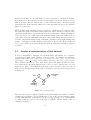
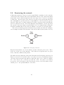
A way of structuring a situation for reasoning under uncertainty is to construct
a graph representing causal relations between events. To simplify the situation,
assume that we have the events {yes, no} for Fuel in tank ?, {yes, no} for Clean
spark plugs?, {full, 12 , empty} for Fuel Meter Standing, and {yes, no} for Start?
These defined outcomes are also called states, this is the name we will use in the
rest of this thesis. We know that the state of Fuel in tank? and the state of Clean
Spark Plugs? have a casual impact on the state of Start Problem? Also, the state of
Fuel in tank? has an impact on the state of Fuel Meter Standing. This is represented
in Figure 3.1.
Fuel
F
CSP
FM
S
Fuel Meter
Standing
Start
Clean Spark
Plugs
Figure 3.1. Car start problem.
The idea is to describe complex relations in a way that makes it possible to calculate
conditional probabilities. As one might expect, one of the biggest challenges when
dealing with Bayesian networks is to model real life systems. It is often difficult
to clarify relations between real events and to estimate which relations could be
considered negligible.
9
3.4
Structuring the network
A Bayesian network is a directed acyclic graph (DAG) consisting of nodes and the
connections between them. An acyclic network has only one way connections which
means that a node with an input from the node layer above can not be an input
to that layer. The direction of the arrows is decided by the system and show how
the causal influence spreads in the net. Causal influence can not spread in opposite
direction. This can be resembled with the Fuel Meter Standing sensor affecting the
fuel level, which is not true. Note that although causal influence can not spread in
the opposite direction, changes in probabilities can. It is natural that reading the
fuel meter standing affects our beliefs on whether or not there is gas in the tank.
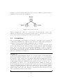
The nodes are named parent and child to help orientate the network. In Figure
3.2 an example is shown. The structure of the net is defined by the system. In every
Prior
nodes
Parent
N1
N2
Parent
N3
Child
Figure 3.2. Converging connection
Bayesian network there are nodes with no parents called the prior nodes. These
nodes are on the top of the structure. Note that not all parent nodes are prior
nodes, only those without own parents.
We shall look at two different connections, Diverging and Converging connection. In
Figure 3.2 nodes N1 , N2 and N3 form a converging connection. Probability changes
can pass between parents only when we know the state of N3 . Take for example
N3 = Sore throat, N1 = Chicken pox and N2 = F lu. If we have a sore throat
we increase our beliefs that we have the flu and decrease our beliefs that we have
chicken pox, i.e. the parents influence each other.
10
In Figure 3.3 N4 , N5 and N6 form a diverging connection. Influence can pass between
children as long as state N4 is unknown.
Parent
N4
Child
N5
N6
Child
Figure 3.3. Diverging connection
Take for example N4 = F uel, N5 = F uel meter standing and N6 = Start. The
influence is not passed on if we know the parent’s state, i.e. the fuel meter standing
do not effect start if we know that we have gas in the tank.
3.5
Probabilities
The network requires probabilities to be assigned to the prior nodes and that all
conditional probabilities are defined for the other nodes. When this information is
available to the net, all probability calculations can be performed.
When determining the probabilities from experiences of the system we insert
noise to the system because the probabilities deviate from the right distribution.
Some noise is accepted but if the probability distribution becomes to noisy the
performance of the net will decrease. Therefore the accuracy of the net will to a
great extent depend on how well the probability distribution are determined. The
principle is illustrated by Example 1.
Example 3.1
Consider the system illustrated in figure 3.1. Let CPS denote “Clean spark plugs”.
The prior probabilities p(F uel in tank = no | ) and p(CP S = no | ) is determined
by experience of the system. If we for example know that the spark plugs often get
dirty we have a high probability for that state. If the car does not start we would like
to know which of the two conditional causes, p(F uel in tank = no | Start = no, )
and p(CSP = no | Start = no, ), are the most probable. Empty gas tank is easy
to check with the fuel meter standing sensor. If the fuel meter standing is working
correctly and shows that there is gas in the tank the Fuel in tank variable can not
explain the fault but CSP can. The fuel meter standing effects the Fuel variable
which in turn effects CSP. The diagnostic conclusion depends on how we set the
prior probabilities for this specific system.
11
In the example above experience of the system is used. If we have a new system we
can implement the experiences received during the research and development into
the Bayesian net. This is very valuable for a mechanic when diagnosing the system.
A mechanic with no experience of the new system can make use of the experience
the developers gained during research. Furthermore, as more experience is gained
throughout the use of the system, this information can be used to further improve
the Bayesian net.
12
Chapter 4
The cost of repair
This section will introduce the cost distribution and the expected cost of repair,
ECR. The ECR is used as a measure of how cost effective a TS-strategy is. In the
final section the TS-problem is defined as an optimization problem.
What we are looking for in a TS-process is to repair a malfunctioning device. This
can be done by performing tests, observations and repair actions until the device is
working properly. But we are not only interested in repairing the device by following
some TS-strategy but rather to follow the best TS-strategy.
In this context the best TS-strategy will not only repair the device but will also do
this by arranging actions in such a way that they make the average TS-cost as low
as possible.
4.1
Cost of repair
The TS-costs include the repair cost CR = (C R1 , C R2 , . . . , C Rn ) which includes
costs arising from repair time, spare parts, configuration changes, software updates
and the cost of repair tools exposed to wear. It also includes the observation cost
CO = (C O1 , C O2 , . . . , C On ) which describes costs arising from determining whether
or not a specific component is causing the system malfunction. There is also the
cost of performing tests CT = (C T1 , C T2 , . . . , C Tm ), where C Tj includes all costs
that are associated with concluding the answer of a specific test Tj . The total cost
of a TS-sequence is simply the cost of all performed observations together with the
cost of performed tests and the cost of the final repair. The total cost of a specific
TS-strategy is not obvious but will be disused later in this chapter.
13
There is also consideration of indirect costs such as logistics costs, costs of not be
able to use the malfunctioning device, costs of developing more accurate diagnostic
systems and so forth. It is also important to notice that the total cost does not
only consist of monetary values but also the cost of potentially loosing a customer’s
loyalty and business due to prolonged repair times. However, these considerations
are not discussed in this text.
4.2
The cost distribution
Let us introduce the probability distribution p(CS ). This probability distribution
shows how probable it is to end up with a certain TS-cost when using a specific
TS-strategy.
Definition 4.1. Assume a TS-strategy S. If CS = (C1S , C2S , . . . , CnS ) were each CiS
is calculated under assumption that fault Fi is present, then p(C S ) is refered to as
the probability distribution of CS for a specific TS-strategy S.
Note that CiS is the cost of the TS-sequence arising from fault in component Xi .
The principle of the cost distribution calculation is illustrated in Example 4.1.
Example 4.1
Assume a subsystem with three components X = (A, B, C) where one of the components is the cause for a malfunction or a system symptom. The cost for observing
and repairing the components as well as their initial fault probabilities are given in
the table below:
Component
A
B
C
Prob.
0.2
0.5
0.3
Obs. Cost
12
17
9
Rep. Cost
40
68
50
Now, let us assume that a suggested TS-strategy for the symptom is to examine
the components in the order (C, A, B), i.e the TS-strategy is S = (C, A, B). To
calculate the cost distribution for this strategy we must compute the total cost of
each possible TS-sequence arising from all possible faults. The cost distribution of
S is given in the table below.
Fault in component:
A
B
C
TS-sequence cost (using S)
61
106
59
The distribution tells us that there is a 20%, 50% and 30% chance to end up with
a repair cost of 61, 106 and 59 respectively, if we follow the actions suggested by S.
14
4.3
The expected cost of repair
As shown above the cost distribution can be used to measure how cost effective a
TS-strategy is. This cost-effectiveness is measured as an expectation of the cost
distribution and will be used as an optimality condition for calculation of cost minimizing TS-strategies.
The expectation E[X] for a discrete stochastic variable X is calculated by
E[X] =
x · p(X = x).
(4.1)
By using the expectation and Definition 4.1 it is possible to introduce the
Expected Cost of Repair, ECR(S|F), which should be interpreted as the expected
cost of repair for a TS-strategy S calculated for all faults F i.e.
ECR(S|F) = E[p(CS )].
(4.2)
The TS-strategy S and faults F will be implied and the expected cost of repair will
be denoted as ECR. Example 4.2 illustrates the ECR calculation.
Example 4.2
The ECR for the cost distribution derived in Example 4.1 can be calculated as
E[p(CS )]=61 × 0.2 + 106 × 0.5 + 59 × 0.3 = 82, 9
So, if we always troubleshoot this particular symptom as suggested by S we will end
up with a average cost of 82,9.
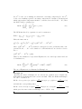
4.4
ECR with separate costs
Since we consider the cost of observing and the cost of repairing as two separated
costs it is necessary to modify Equation 4.2. Heckerman proposes in [2] a way
to calculate the ECR with different considerations for CR and CO . Heckerman’s
proposal also makes it possible to calculate the ECR without using the total cost of
all possible TS-sequences. Dividing the ECR will improve the resolution of the ECR
calculations and will also provide better possibilities of manipulation. Heckerman’s
proposition assumes that a observation always concerns a specific component and
that the answer always reveals whether the component is broken or not. The cost
COi should hence be considered as the cost of determining whether some repair Ri
is necessary, before Ri is actually performed.
15
Let C Oi be the cost of making observation Oi concerning component Xi . Let C Ri
be the cost of making repair Ri concerning component Xi . Assume a TS-strategy S
which suggest that components should be considered in order X1 , X2 , . . . Xn , then
the ECR could be calculated as,
⎛
⎞
n
i−1
⎝1 −
pj ⎠ C Oi + pi C Ri .
(4.3)
ECR =
i=1
j=1
The ECR introduced by equation 4.3 can be rewritten as
n
Oi +
Ri
ECR = ni=1 1 − i−1
j=1 pj C
i=1 pi C .
Write the first term as
n
n i−1
Oi =
ok
ok
ok
Oi
i=1 1 −
j=1 pj C
i=1 p(X1 , X2 , · · · , Xi−1 )C ,
ok ) should be interpreted as the probability that comwhere p(X1ok , X2ok , · · · , Xi−1
ponents X1 , X2 , · · · , Xi−1 were found to be OK and that we are about to observe
Oi , i.e.
ok ) = p(O ).
p(X1ok , X2ok , · · · , Xi−1
i
Thus, by the definition of expectation Equation 4.3 is a valid expectation and can
be formulated as,
ECR =
n
i=1
pi C Ri +
n
p(Oi )C Oi = E[CO ] + E[CR ]
(4.4)
i=1
The use of Equation 4.3 is illustrated in Example 4.3.
Example 4.3
By using the values of Example 4.1 we can now use equation 4.3 to calculate the
ECR without calculating the total cost for each fault. Thus, the ECR from Example
4.1 can be calculated as:
p2
p3
C R2 )+(1−p1 −p2 )(C O2 +
C R3 )
ECR = C O1 +p1 C R1 +(1−p1 )(C O2 +
1 − p1
1 − p1 − p 2
and with the corresponding values:
0, 2
0, 5
ECR = 9+0, 3×50+(1−0, 3)(12+
×40)+(1−0, 3−0, 2)(17+
×68)
1 − 0, 3
1 − 0, 3 − 0, 2
which gives the same result as in Example 4.2 i.e. ECR = 82,9
16
4.5
Minimizing ECR
The ECR gives a measure for how good a TS-strategy is. As mentioned before a
good TS-strategy is a TS-strategy that gives a low ECR. Therefore when suggesting
a strategy it should be under the condition that it minimizes ECR. Thus we need
to find the TS-strategy S which solves the optimization problem,
min ECR(S).
(4.5)
Heckerman [2] suggests that by ordering components Xi by their efficency index
ef (Xi ) =
pi
,
C Oi
(4.6)
in descending order a TS-strategy that solves Equation 4.5 is gained.
If two components have the same fault probability (conditioned on the current state
of knowledge) but different observation costs, then we choose to observe the component with the lowest observation cost and vice versa. A proof of the efficiency index
can be found in Heckerman [2].
The efficiency index tells us in which order we should observe components under our
current state of knowledge. However, if our beliefs change during troubleshooting
then the efficiency index of each component needs to be updated since the probabilities change. Efficiency index calculation is illustrated by Example 4.4.
Example 4.4
Again, consider Example 4.1. The efficiency ranking for components A,B,C is given
below:
Component
A
B
C
Prob.
0.2
0.5
0.3
Obs. Cost
12
17
9
Efficiency index
0.017
0.029
0.033
Thus, the TS-strategy based on the efficiency index should observe components in
the order S = (C, B, A). By using Equation 4.3 we gain the expected cost of repair
for the suggested order, ECR = 80,3. So, we will lower our TS-costs by 2,6 on
average by following the efficiency ranking instead of than the strategy suggested in
Example 4.1.
17
Chapter 5
Troubleshooting algorithms
To determine a troubleshooting sequence the information from the Bayesian network
and the component data needs to be combined. This information processing is handled by the troubleshooting algorithms. The different algorithms use the available
information in different ways and are preferable for different purposes.
5.1
Introduction to troubleshooting algorithms
The ideal TS-algorithm would suggest TS-steps according to an optimal strategy.
The optimal strategy should guarantee that by following the suggested steps one
would on average save as much money possible on every TS-scenario.
To find the optimal TS-strategy for a given system one has to calculate the ECR
for all possible strategies and choose the strategy with the lowest ECR. However,
the troubleshooting problem is proven to be very hard to optimize (NP-complete,
proven in [7]). To calculate the ECR for all possible strategies for any non naive
model is a overwhelming task. Thus, algorithms that propose suboptimal strategies
are required for any practical implementation.
18
5.2
Algorithm 1: The greedy approach
The efficiency index is introduced in Section 4.5 and is considered to be the best
strategy search criterion. By using the efficiency index a suboptimal TS-strategy can
be found. A proof for this can be found in [4]. If we should approach a troubleshooting problem in a greedy way we should make component observations according to
the efficiency index in descending order. A strategy based on the greedy approach is
suboptimal as discussed in [4]. The strategy is optimal under the assumptions given
in Section 2.2 together with the assumption that there are no questions and that
the components are independent. A proof for this is also given in [4]. The greedy
approach extracts the component probabilities and their corresponding observation
costs and calculates the efficiency ranking for each component. The suggested strategy is then given as the descending order of component efficiency ranking. The
algorithm flowchart is given in Figure 5.1.
Component
cost information
Compute efficiency index
for all components
Sort components by
descending ef.
Bayesian net
Return sorted components
Exclude observed
component
Ok
Observe first
comp. in
order
Broken
New order
Figure 5.1. The greedy algorithm flowchart.
19
Repair. End
troubleshooting
5.3
Algorithm 2: The greedy approach with updating
The greedy algorithm has a initial information approach i.e. the strategy is only
based on the initial information. If our belief about the component probabilities
change during observation the greedy algorithm will not consider this there is no
feedback from the Bayesian network to the algorithm. Therefore a way to improve
the performance of the greedy algorithm is to introduce probability updating. This
makes the greedy algorithm consider changes in component probability and by doing
so creating a more adaptable algorithm. The updating also relaxes the independence
requirement of the non updating greedy algorithm. The flowchart for the greedy
algorithm with probability updating is given in Figure 5.2
Component
cost information
Compute efficiency index
for all components
Sort components by
descending ef.
Bayesian net
Return sorted components
Information
update
Exclude observed
component
Ok
Observe first
comp. in
order
Broken
Repair. End
troubleshooting
Figure 5.2. The greedy algorithm with probability updating flowchart.
20
5.4
The value of information
The algorithms described above uses observations as the only source of new information. They rely on good initial information of the system such as pre performed tests
and isolated symptoms. To further improve the performance of the TS-algorithms
the use of information must be considered. To do this we need a measure for the
value of information.
To supply the algorithms with new information we introduce tests. The information
supplied by the tests should be used in the best way possible. Since the goal of a
TS-algorithm is to suggest a cost minimizing TS-strategy, a measure for how to value
available tests must be defined. This value is referred to as the ECRT (Expected cost
of repair after test) for a specific test. The ECRT is calculated as the expectation of
ECR for the possible test outcomes together with the test cost. This gives a value
for how much the troubleshooting will cost on average when performing a test. The
ECRT is given by Equation 5.1.
ECRTj =
Q
p(Tj = qi | ) × ECR(Tj = qi | ) + C Tj
(5.1)
i=1
the sum is over q1 , q2 , . . . , qQ were Q denotes the number of all possible outcomes
for test Tj and C Tj is the cost of test Tj .
In this thesis only test with two possible outcomes will be considered. This simplifies
Equation 5.1 to
ECRTj = p(Tj = q1 | )×ECR(Tj = q1 )+p(Tj = q2 | )×ECR(Tj = q2 )+C Tj (5.2)
It is important to denote that the probability p(Tj = qi | ) is dependent on the
current knowledge of the system and therefore must be extracted from the Bayesian
net for each evaluation of ECRT. The outcomes q of a test Tj should be interpreted
as the possible states of Tj . For instance, a test T : Is there gas in the tank? might
have the states q1 = Y es and q2 = N o.
21
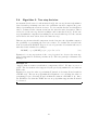
5.5
Algorithm 3: One step horizon
The one step horizon TS-algorithm is based on the greedy approach but incorporates
the possibility to perform tests during troubleshooting. Using the ECRT definition
given by Equation 5.1 the algorithm compares the value of observing the component suggested by the greedy approach with the value of performing a test. This
comparison is done by calculating the greedy ECR and the ECRT for all available
test and choosing the action which corresponds to the lowest value of ECR or ECRT.
The one step horizon algorithm compares the ECRT with the ECR for each action.
The comparison makes the algorithm decide which test if any is best to perform as
the next action. If the one step horizon algorithm has access to well discriminating test it should isolate the faulty component faster and cheaper that the greedy
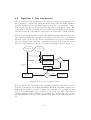
approach. The flowchart for the one step horizon algorithm is given in Figure 5.3.
Bayesian net
Component
Cost
cost
information
information
Calculate ECR
ECR>ECRT?
No
Calculate ECRT for all test
Information
update
Perform test with
lowest ECRT
Exclude observed
component
Ok
Observe
comp.
Yes
Broken
Repair. End
troubleshooting
Figure 5.3. The one step algorithm flowchart.
However, the one step algorithm is biased towards performing tests. This bias arises
from the comparison between ECR and ECRT. When the algorithm compares the
ECR with the ECRT it actually compares the possibility of performing the test
now or never, thus making more reasonable to choose the test. This should not be
confused with the actual possibility of performing the test later but rather as how
the algorithm values the test at the current action. This bias is further discussed in
[3].
22
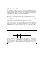
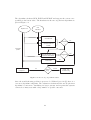
5.6
Algorithm 4: Two step horizion
As mentioned in Section 5.5 and motivated in [3], the one step horizon algorithm is
biased towards performing tests since the evaluation criterion compares the possibility of performing the test now or newer. To even out this bias the test should not
only be evaluated at the current action but also after the next observation. This is
referred to as the two step horizon technique and is introduced in [3]. In the two
step algorithm the comparison for making a test is made with respect to the current
action and to the next action, hence the name two step.
This two step horizon should compensate for the bias since the algorithm compares
the possibility of performing the test now or later. To evaluate the test after the
next observation the ECROT (Ecpected cost of repair after observation and test) is
introduced and calculated according to
ECROTj = pi × (ECRTj ) + (1 − pi ) × C Ri + C Oi
(5.3)
Equation 5.3 is an expectation of the cost of repair if we observe the next suggested component Xi and then perform test Tj . The basic principle is illustrated by
Example 5.1.
Example 5.1
Suppose that we want to troubleshoot components A, B, C. We have access to a
test T . The observation order suggested by the greedy algorithm is B, A, C with an
ECR of 20.
Equation 5.1 gives the value of performing T instead of observing B and results in
a ECRT of 18. The two step algorithm uses Equation 5.3 to calculate the value of
performing T after observing B and calculation results in a ECORT of 17. Since
the ECORT is less than the ECRT the two step algorithm suggests that B should
be observed.
23
The algorithm calculates ECR, ECRT and ECROT and suggests the action corresponding to the lowest value. The flowchart for the two step horizon algorithm are
given in Figure 5.4
Bayesian net
Component
Cost
cost
information
information
Calculate ECR
ECR>ECRT
?
Calculate ECRT for
all tests
Yes
Information
update
Yes
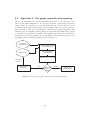
Calculate ECROT for all
tests were ECR>ECRT
Ok
Observe
comp.
ECRT>ECROT
?
No
Perform test with
lowest ECRT
Exclude observed
component
No
Broken
Repair. End
troubleshooting
Figure 5.4. The two step algorithm flowchart.
Since the troubleshooting problem is proven to be NP-hard (proof in [7]) there is a
concern of algorithm complexity. The evaluation calculation in the two step horizon
algorithm becomes more demanding for larger systems and in particular systems
connected to many tests with a large number of possible outcomes.
24
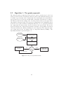
Chapter 6
Simulation models
We want to apply the TS-algorithms on different types of network models to evaluate
how the algorithm performance depends on the model. To evaluate the algorithms
we are interested in two types of models;
• A real life model - to motivate the use of the algorithms in real life.
• Evaluation models - to investigate the behaviour of the algorithms.
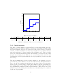
6.1
HPI injection system model
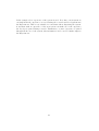
In [1] a Bayesian model of a diesel motor injection system (HPI) is derived. This
model will be used as the real life model. Table 6.1 and Table 6.2 gives the model
parameters. Figure 6.1 summarizes the model structure.
Comp.name
Fuel tank
Filter housing
Fuel armature
Fuel filter
Overflow valve
Fuel shut off valve
Connection nipple
Fuel hose
Fuel pump
Fuel manifold
Node name
FT
FH
FA
FF
OV
FSV
CN
FHO
FP
FM
Prob. (%)
0,09
0,3
0,7
1,4
2
0,9
0,8
0,4
0,8
0,3
Obs.Cost (sek)
55
550
330
495
440
550
330
385
1100
1210
Table 6.1. Component parameters.
25
Rep.Cost (sek)
200
2300
1700
500
320
780
260
120
3750
3200
Test
Air in system
Fuel tank
Low pressure
Cost [sek]
300
10
100
Table 6.2. Test costs for the HPI model.
Constr.
FT
Fuel
FH
FA
FF
OV
FSV
Low
pressure
CN
FHO
Air in
system
D005
Figure 6.1. The HPI model structure.
26
FP
FM
6.2
Evaluation models
6.2.1
Evaluation model 1
If we want to evaluate the impact of certain parameters or structures on the algorithms we can not use the HPI model since the parameters and the model structure
are fixed. Thus, another model is required. Figure 6.2 illustrates the evaluation
model 1. The parameter settings are given in Table 6.3.
Figure 6.2. Evaluation model 1.
Parameter
Prob. for A
Prob. for B
Prob. for C
Obs.cost for A
Obs.cost for B
Obs.cost for C
Rep.cost for A
Rep.cost for B
Rep.cost for C
Test cost for TA B
Test cost for TA C
Test cost for TB C
Type
Probability [absolute]
Probability [absolute]
Probability [absolute]
Cost [sek]
Cost [sek]
Cost [sek]
Cost [sek]
Cost [sek]
Cost [sek]
Cost [sek]
Cost [sek]
Cost [sek]
value
0.1
0.2
0.3
700
900
1100
30
40
50
21
23
22
Table 6.3. Simulation parameters for evaluation model 1.
27
The parameters of evaluation model 1 is not fixed and may be set to arbitrary
values. However, during simulation, the parameters is chosen according to Table 6.3
as standard model settings.
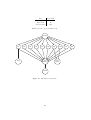
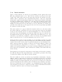
6.2.2
Evaluation model 2
Both evaluation model 1 and the HPI model have the same network structure. To
evaluate the advantages of the more complex algorithms a model with stronger component dependencies are required. In Figure 6.3 evaluation model 2 is presented. To
model direct component dependencies constitutes a problem since this means that a
node in the component layer influences another node in the same layer. This creates
cycles in the network.
To avoid creating cycles we propose to represent all components with two nodes.
One node is used to handle component probability and works in the same way as
the nodes in the other models. The other node is to model the influence this component has on other components. Since both nodes have the same meaning in practice
they are treated the same way i.e. both nodes will always be in the same state.
Evaluation model 2 is illustrated by Figure 6.3 and the model parameters are given
in Table 6.4.
We will consider two types of component dependence, positive and negative. Positive
dependence increases a belief. A negative dependence decreases the belief. For
example, if component A has a positive influence on C the evidence that A is ok will
increase our belief that C is ok and a negative influence would decrease our belief
about C.
28
Figure 6.3. Evaluation model 2.
The nodes named Obs. supplies the component probabilities to the algorithms. The
nodes named inf. represents the influence of the corresponding component on other
components. For instance, when calculating the efficiency index of A we use the
probability supplied by Obs. A and inf. A represent the influence our knowledge
about A has on C.
29
Parameter
Influence from A to C
Influence from C to B
Prior prob. for A
Prior prob. for B
Prior prob. for C
Obs.cost for A
Obs.cost for B
Obs.cost for C
Rep.cost for A
Rep.cost for B
Rep.cost for C
Test cost for TA B
Test cost for TB C
Type
Probability [absolute]
Probability [absolute]
Probability [absolute]
Probability [absolute]
Probability [absolute]
Cost [sek]
Cost [sek]
Cost [sek]
Cost [sek]
Cost [sek]
Cost [sek]
Cost [sek]
Cost [sek]
value
+ 0.6
+ 0.7
0.31
0.32
0.37
100
200
300
10
20
30
90
66
Table 6.4. Simulation parameters for evaluation model 2.
30
Chapter 7
Simulation
Simulation and validation of TS-algorithms poses a potential problem. The Bayesian
network and the algorithms evaluates actions based on certain criteria (information)
and therefore when evaluating the behaviour of a TS algorithm all possible configurations of troubleshooting scenarios must be considered. In the evaluations below, a
simulation is done for fault in every model component. By using the cost distribution
an expectation for the proposed strategy is calculated.
7.1
General performance
In this simulation the ECR for all algorithms are calculated when applied to the
different models. The general model settings given in Chapter 6 are used.
7.1.1
Simulation results for the HPI model
Table 7.1 shows the ECR performance of the diffrent algorithms on the HPI model.
Algorithm
Greedy
Greedy with updating
One step
Two step
ECR [sek]
2463
2463
2381
2381
Table 7.1. Simulation results for the general simulation of the HPI model.
31
7.1.2
Simulation results for evaluation model 1
Table 7.2 shows the ECR performance of the different algorithms on evaluation
model 1.
Algorithm
Greedy
Greedy with updating
One step
Two step
ECR [sek]
806
806
488
488
Table 7.2. Simulation results for the general simulation of evaluation model 1.
7.1.3
Simulation results for evaluation model 2
Table 7.3 shows the ECR performance of the different algorithms on evaluation
model 2.
Algorithm
Greedy
Greedy with updating
One step
Two step
ECR [sek]
549
513
349
349
Table 7.3. Simulation results for the general simulation of evaluation model 2.
32
7.1.4
Result comments
Table 7.1 shows that the one and two step algorithms perform equally well for the
HPI and evaluation model 1 case. Also the two versions of greedy give the same
results. The equal result of the greedy approaches and the one and two step algorithms could be explained by the component independence. Since the component
independence makes new information update the component probabilities uniformly
the efficiency ranking will be unchanged i.e. the ratio between efficiency index of the
components will be constant. Since there is no additional gain in information when
making observations the two step will behave as one step. Both the one and two step
performs better than the greedy approach since the test incorporating algorithms
are quicker to isolate the fault.
The same result is to be expected from the structure model case. One notices that
the relative difference in ECR for the two greedy approaches and step algorithms
is larger for the structure model case than for HPI model case. Since the structure
model has better discriminating tests than the HPI model the one and two step
algorithms should isolate the fault more quickly than in the HPI model case. Is is
reasonable to say that the performance of the one and two step algorithms should
improve with the increase of well discriminating tests and vice versa.
In the dependence model case the updating greedy algorithm performs better than
the simple greedy approach. This is probably due to the standard negative influence
setting of the model. At the start of troubleshooting the greedy algorithm determines a strategy and newer changes it. However, the negative influence changes our
belief about the next component to be observed i.e. a large probability becomes
smaller and a small probability becomes larger and thus changing the internal relation between the probabilities. This overthrows the validity of the initial efficiency
index ordering.
The updating greedy approach compensates for this change in belief and recalculates
the efficiency index for all components when a observation is performed. By doing
so assures the validity of the efficiency index ordering.
The lack of difference in the one and two step algorithms is unfortunate. Negative
influence makes a component observation serve as minor test since the observation
changes the probability of other components. This should make the two step algorithm to perform observations when the one step prefers to perform a test. The most
probable explanation for the similar result of one and two step is that the dependence
model is too small and does not constitute a good simulation model. Future simulations should incorporate more complex dependence models with different structures
to map the behaviour of the one and two step algorithms.
33
7.2
Dependence
The aim of the first dependence simulation is to investigate how component dependency affects algorithm performance. The aim of the second simulation is to
investigate how the test cost affects the performance of the one and two step algorithms. All simulations in this section is done using the dependence model.
7.2.1
Algorithm dependence performance
The influence from A to C is varied from -0.30 to 0.30 in steps of 0.10 and the
dependence from B to C is set to zero. A influence of 0.30 means that the probability
of C increases by absolute 0.3 (from the initial probability for C of 0.6 to a maximum
of 0.9). A influence of -0.30 means that the probability of C decreases by absolute
0.3 (from the initial probability for C 0.6 to a minimum of 0.3). ECR for each
algorithm is registered for each step. Table 7.4 and Table 7.5 illustrates the effect
of dependence on the algorithm ECR performance.
Algorithm
Greedy
Greedy w.up
One step
Two step
ECR(0)
550
439
349
349
ECR(0.1)
550
439
349
349
ECR(0.2)
550
439
349
370
ECR(0.3)
550
439
349
370
Table 7.4. Simulation results for positive dependence.
Algorithm
Greedy
Greedy w.up
One step
Two step
ECR(0)
550
439
349
349
ECR(-0.1)
550
461
349
349
ECR(-0.2)
550
461
349
349
ECR(-0.3)
550
461
349
349
Table 7.5. Simulation results for negative dependence.
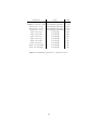
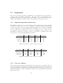
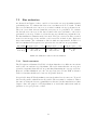
7.2.2
Test cost influence
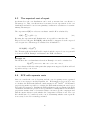
The general settings apply in this simulation except for the test settings. The test
cost for both tests are varied from 50 sek to 100 sek in steps of 10 sek. Table 7.6
together with Figure 7.1 illustrates the simulation results. In Figure 7.1 the one step
algorithm is illustrated with a straight line and the two step algorithm is illustrated
with a dotted line.
34
400
390
380
ECR [sek]
370
360
350
340
330
320
310
300
50
60
70
80
Test cost [sek]
90
100
Figure 7.1. Test cost influence.
Algorithm
One step
Two step
ECR(50)
308
308
ECR(60)
319
319
ECR(70)
329
370
ECR(80)
340
370
ECR(90)
349
370
ECR(100)
360
370
Table 7.6. Simulation results for the test cost simulation.
7.2.3
Result comments
The effect of positive influence is shown in Table 7.4 and shows that the only algorithm affected by the change in influence is the two step algorithm. Remember that
the positive influence increases our belief in the same direction as the observation
outcome, so when the influence becomes large enough, two step considers that the
gain in observation to be larger than the gain of making a test. This is possibly
due to the additional information gained when making a observation is larger than
the gain of performing a test. However, the test in the dependence model is well
discriminating and cheap which makes the two step algorithm to perform worse than
the one step.
The only algorithm affected by the negative influence is the updating greedy approach. In the positive influence case the belief did not change during troubleshooting i.e. the efficiency ranking after updating gave the same result as before updating.
In the negative case this changes. The negative influence flips the probability relations and by doing so also changes the efficiency index ordering. The one and two
step algorithms are unaffected by the negative influence. This could be due to the
information gained by making observations is to non-discriminating to be considered
by the two step algorithm.
35
Table 7.6 shows the change in ECR for one and two step when gradually increasing
the test cost. The ECR for one step increases linear with the test cost since the
algorithm always performs one of the tests. The two step performs test for the
initial test cost and for the firs iteration. After this the two step approach only
performs observations and making the ECR increase in comparison with the one
step ECR. The decision made by two step to only perform test when the test costs
passes the 70 line could be due to the positive influence in the simulation model. In
this simulation the two step perfumes worse than the one step for all test costs but
this is probably due to the model. Thus, as suggested in the general simulation case
to further investigate the properties of the one and two step mode advanced models
are required.
36
7.3
Bias evaluation
As discussed in Chapter 5 there could be a bias in the one step algorithm towards
performing tests. To evaluate this bias a test cost limit needs to be found. To find
the test cost limit the test cost is set to a value for which one step performs a test.
The test cost is then increased until the test seizes to be performed. To evaluate
the bias the test cost is set to the lower bound of the test cost limit i.e. the test is
preformed by one step. If there is a bias the two step should not perform the test.
For this simulation evaluation model 2 is used. The test cost for test TBC is varied
from 57 to 61 in steps of two and the cost for test TAC is fixed at 105. Both test
have 0 uncertainty. The evaluation is done for fault in component B. In Table 7.7
the bias simulation TS-sequences are given for the one and two step algorithms.
Algorithm
One step
Two step
Sequence(C TBC = 57)
TBC , TAB , B
TBC , TAB , B
Sequence(C TBC = 59)
TBC , TAB , B
TBC , TAB , B
Sequence(C TBC = 61)
TBC , TAB , B
A, B
Table 7.7. Simulation results for the bias simulation.
7.3.1
Result comments
The TS-sequences illustrated by Table 7.7 shows that there is a difference in actions
used by the one and two step algorithms. The table shows that the one step uses
test more frequently than the two step and thus illustrating the one step test bias.
However, in this simulation case, the one step bias gives a lower ECR as shown i
Table 7.6 but this should not be true for all possible models.
It is probable that all TS-algorithms is associated with a bias of some sort. To avoid
the bias all possible evaluations for all possible TS-cases must be evaluated. This is
the same as doing the discrete optimization as discussed in the introduction of this
chapter. Since the purpose of TS-algorithms is to avoid this cumbersome task we
just have to accept a presence of bias.
37
7.4
Complexity
The complexities of the algorithms are evaluated by taking the time it takes matlab
to run the algorithm. This is not a out trough complexity analysis but since the
algorithm programs are similarly implemented the simulation should give a general
picture of the complexity. The simulation is done using the structure model. Keep
in mind that the structure model is a very simple Bayesian net with only six active
nodes. Table 7.8 gives the comlexity simulation results.
Algorithm
Greedy
Greedy with updating
One step
Two step
Exe.time (sec)
4,73
6,35
23,97
68,05
Table 7.8. Algorithm complexity.
7.4.1
Result comments
It is no surprise that the algorithm complexity increases with the more advanced
approaches. The techniques used by one and two step are computational demanding
for lager systems since the number of evaluations increases fast with more tests
and components. When designing a troubleshooting system this is an important
consideration. If the system should be a tool for a mechanic or support personnel
the calculations must be done in real time. The computational aspect could probably
be avoided by making good models and use fast updating software.
38
7.5
Simulation conclusions
In Section 7.1 the value of tests becomes clear. In all of the simulations the one and
two step algorithms gives a better cost performance. However, the updating greedy
approach performs relatively well. Generally it could be stated that the presence
of test makes the troubleshooting process faster and cheaper. A trouble shooter
should therefore try to design well discriminating tests if the application is a system
with time consuming observations. For easy observable systems the updating greedy
approach is a reasonable choice.
39
Chapter 8
Conclusions and discussion
The approach of using Bayesian networks serves as a possible solution to the problems of traditional troubleshooting. The properties of the Bayesian network makes
it possible to quickly modify models and thereby overcoming the problem with the
variety of component configurations in modern trucks. To model the different truck
systems as a Bayesian network is a huge task and requires information that is usually
not available. A possible solution is to consider the Bayesian approach early in the
development of new systems.
Four TS-algorithms have been derived and evaluated using three diferent simulation
models. The troubleshooting algorithms perform well on the HPI model and illustrates that the proposed techniques constitutes a possible future implementation.
There are still more investigations to be made, especially regarding network structure and the effect on the different algorithms. The issue of algorithm complexity
should also be investigated further.
Other considerations are the possibility to use the TS-algorithms as a analytic tool to
determine specifications for tests and component accessibility. The algorithms could
also be used to analyze were troubleshooting research effort should be focused. For
example, if a component is replaced. If the Bayesian system model exists one can
determine the effect of an new test and the maximum test costs.
40
Chapter 9
Recommendations
The results presented in this thesis show that the approach of probabilistic troubleshooting has a great potential in the heavy duty truck maintenance area. Future
research should concentrate on developing better and faster algorithms. Since the
bottleneck of the approach is the derivation of Bayesian models from real life systems, future work should focus on this area to produce better ways of generating
Bayesian models. Other possible approaches could be to implement evolutionary
algorithms. These algorithms improve over time and should, with enough training,
be able to approach the optimal solution for a certain system.
41
References
[1] J. Andersson. Minimizing troubleshooting costs - a model of the hpi injection
system. Master’s thesis, Department of automatic control, Royal Institute of
Technology, Stockholm, Sweden, December 2006.
[2] Koos Rommelse David Heckerman, John S. Breese. Decision theoretic troubleshooting. 1995.
[3] Brian Kristiansen Helge Langseth Claus Skaanning Jiri Vommel Marta Vomlelova Finn V. Jensen, Uffe Kjaeulff. The sacso methodology for troubleshooting
complex systems.
[4] Finn V. Jensen Helge Langseth. Decision theoretic troubleshooting of coherent
systems.
[5] M. Jansson. Fault isolation utilizing bayesian networks (internal scania version).
Master’s thesis, Department Department of Numerical Analysis and Computer
Science, Royal Institute of Technology, Stockholm, Sweden, January 2004.
[6] Finn V. Jensen. Bayesian Networks and Decsion Graphs. Springer, 2001.
[7] J.Vomlel M. Vomlelova. Troubleshooting: Np-hardness and solution methods.
42