1
Examples
CHAPTER 9
RepTile Examples
Expert
In general, the steps involved in using RepTile surfaces consist of first creating a
RepTile surface property within TracePro and then applying that property to a
plane surface in your TracePro model. All the examples in this section are similar
in construction. You should choose an example that is most like the model you
wish to create and follow through the steps for creating the example.
Fresnel lens
In this example we will create a Fresnel lens. Some of the important features of a
Fresnel lens are shown in Figure 9.1
.
FIGURE 9.1 - Important construction features of positive and negative
Fresnel lenses.
In order to begin analyzing a Fresnel lens, you will need to acquire data about the
desired facet angles. If you are analyzing a lens that has already been fabricated,
this data will be available from the manufacturer. If you are analyzing a Fresnel
lens that is in its design stage, you will have to get the facet angle data from
calculations (possibly from a specialized optical design program) outside of
TracePro.
For purposes of this exercise, we have supplied an example file containing facet
angle data. The data for the angular facets of the Fresnel lens example is
contained in the TracePro\Examples\Demos\Fresnel Lens Arcsecs.txt file. This
text file contains one whole number per line – the number is the Fresnel lens facet
angle in arcseconds. In order to use this file, we will need to convert the angles to
degrees. To examine this file, open it using a spreadsheet program such as
Microsoft Excel. The facet angles increase from the center to the edge of the lens.
In order to calculate the minimum thickness we need for the substrate, we need to
know the largest facet angle. This is the last angle in the file. You can quickly go to
the last row in the spreadsheet in Excel by pressing <Ctrl - ↓> on your keyboard.
The Excel screen should look like Figure 9.2, showing that there are 333 rows in
the spreadsheet and the last facet angle is 171682 arcsec or 47.68944 degrees.
Assuming that each facet has a width of 0.5 mm, the depth of the last facet is 0.5
mm x tan(47.68944°) = 0.549 mm. We can make the substrate 2 mm thick, and
Examples
the last facet will still have a base thickness of almost 1.5 mm (substrate thickness
– tallest facet height = base thickness).
FIGURE 9.2 - The Fresnel Lens Arcsecs.txt file as it appears in Microsoft
Excel.
First we will create a RepTile Surface property that describes the Fresnel lens.
Open the Reptile Property Editor by selecting Define|EditPropertyData|
RepTile Properties. The editor appears as in Figure 9.3.
FIGURE 9.3 - The RepTile Property editor with no property selected.
9.2
TracePro 4.1 User’s Manual
RepTile Examples
To add the new property:
1. Press Add Property, and enter a name, for example Fresnel Lens Example,
2. select Fresnel from the Geometry Type drop-down list in the pop-up dialog,
3. select Rings from the Tile Type drop-down list in the dialog,
4. select Variable Rings from the Variation Type drop-down list in the dialog,
5. press OK to create the property.
The RepTile Property Editor will display the property and provide additional inputs
as shown in Figure 9.4.
FIGURE 9.4 - A template for the Fresnel Lens Example RepTile property.
6. Continue to enter the property data by entering 0.5 in the Ring Width box (the
ring width in mm).
We now have a template for creating the Fresnel Lens RepTile property. To fill in
the facet angle and draft angle data, we will export this property to a text file and
use a spreadsheet program.
To export the property, first select File|Save to save the property, then select
File|Export Property to save the property in a text file. Open the text file using
a spreadsheet program (Microsoft Excel was used in this example). The opened
file should appear as in Figure 9.5
TracePro 4.1 User’s Manual
9.3
Examples
FIGURE 9.5 - The Fresnel Lens Example RepTile property exported text file
after opening in Excel.
9.4
TracePro 4.1 User’s Manual
RepTile Examples
With the Fresnel Lens Arcsecs.txt file open in Excel, make a second column that
is calculated from the first column. The second column should be the facet angle
in degrees, obtained by dividing the first column by 3600. The first few rows of the
Fresnel Lens Arcsecs.txt file should appear as in Figure 9.6.
FIGURE 9.6 - The Fresnel Lens Arcsecs file with a second column
containing facet angles in degrees.
TracePro 4.1 User’s Manual
9.5
Examples
Select the entire column B, copy it, and paste it to cell A19 of the Fresnel Lens
Example property file using Paste Special and specifying Values. (You can select
the column quickly by selecting cell B1 in Fresnel Lens Arcsecs and pressing
<Shift - Ctrl - ↓> to select the column). Enter an angle of 2 in the second column
for the Draft Angle. Each facet can have a different angle but we will use a
constant 2 degrees for this example The property should appear in Excel as
shown in Figure 9.7
.
FIGURE 9.7 - The completed Fresnel Lens Example as shown in Excel.
9.6
TracePro 4.1 User’s Manual
RepTile Examples
Now save the Fresnel Lens Example.txt file from Excel and close it. Switch back
to TracePro and select File|Import Property with the RepTile Property Editor
open. Open the Fresnel Lens Example.txt file to import it. The editor window
should appear as in Figure 9.8.
FIGURE 9.8 - The completed Fresnel Lens Example property after importing
into the Property Editor.
This completes the definition of the Fresnel Lens Example in the Property Editor.
Close the Property Editor, and choose to save your data when the appropriate
pop-up window appears.
TracePro 4.1 User’s Manual
9.7
Examples
Now we are ready to make an object and apply the RepTile property we have just
created. First we need to figure out the dimensions the object should have. We
already know that it should be 2 mm thick. We also know that there are 333 facets
of width 0.5 mm, so the radius of the outermost facet is 333 x 0.5 mm = 166.5 mm.
If we use a square boundary for the Fresnel lens, the largest it can be is 166.5 mm
x 2 = 235 mm on a side. We also must have a margin around the RepTile
Surface cell boundary to allow rays to escape properly. Therefore we will make an
object that is 240 mm x 240 mm, and 2 mm thick.
7. In TracePro, using the Insert|Primitive Solid dialog box, insert a block
with dimensions as shown in Figure 9.9.
FIGURE 9.9 - Insert a block into a TracePro model as a substrate for the
Fresnel lens.
8. Using the Apply Properties dialog box, apply the material property pmma from
the Plastic catalog to the block.
9. Now select the –z surface of the block and apply the RepTile surface property
using the RepTile tab in the Apply Properties dialog box. Fill in the values
shown in Figure 9.10.
This puts the center of the Fresnel lens at the center of the block surface.
9.8
TracePro 4.1 User’s Manual
RepTile Examples
FIGURE 9.10 - Insert a block and apply the Fresnel Lens Example RepTile
property to it.
The Fresnel lens is now complete. Note that there will be no visual indication in
the model window that the RepTile surface properties have been applied unless
the View|Display RepTiles option is enabled. The System Tree will show the
Fresnel Lens Example property on the appropriate surface. The facets are
defined over a 235 mm x 235 mm square area within a 240 mm x 240 mm
surface.
Next, we’ll trace some rays through the Fresnel lens.
10.Define a square grid of rays 119 x 119 mm half-widths with a rectangular grid
of 100 x 100 rays as shown in Figure 9.11.
TracePro 4.1 User’s Manual
9.9
Examples
The completed ray-trace is shown in Figure 9.12. We see that the focal length of
this lens is about 310 mm.
.
FIGURE 9.11 - Modified portion of Grid Source dialog for Rectangular
raytrace.
FIGURE 9.12 - Completed ray-trace of Fresnel lens example.
9.10
TracePro 4.1 User’s Manual
RepTile Examples
Conical hole geometry with variable geometry, rectangular tiles and
rectangular boundary
In this example we will create a surface tiled with conical holes and rectangular
tiles. We will create a conical hole property with the following dimensions:
• Cone end radius = variable by row, from 0.1 mm to 0.2 mm in steps of 0.001
mm.
•
•
•
•
•
Cone height = 0.03 mm.
Cone angle = 0.
Chamfer height = 0.02 mm.
Chamfer angle = 50°.
Rectangular tiles, 0.25 mm x 0.25 mm.
These dimensions dictate that there will be 101 rows. Each row is 0.25 mm high,
so the total “y height” of the tiles will be 101 x 0.25 mm = 25.25 mm.
Now we will create the RepTile surface property.
1. Open the RepTile Property Editor by selecting
Define|EditPropertyData|RepTile Properties. The editor appears as in
Figure 9.3 on page 9.2.
2. Press Add Property and enter a name, for example Conical Hole Example,
3. select Cone from the Geometry Type drop-down list,
4. select Rectangles from the Tile Type drop-down list,
5. select Variable rows from the Variation Type drop-down list,
6. and click OK. (See Table 9.13)
FIGURE 9.13 - Enter New RepTile Property dialog for Conical Hole Example.
7. In the Tile Parameters area, enter 0.25 for both the Width and Height values.
8. Click the Bump button and observe that it changes to Hole, specifying “hole”
geometry.
TracePro 4.1 User’s Manual
9.11
Examples
9. Enter the geometry values above into the appropriate columns in the table.
The entries should appear as in Figure 9.14.
FIGURE 9.14 - Completed template for Conical Hole property example.
We now have a template for creating the Conical Hole property. To fill in the
geometry data, we will export this property to a text file and use a spreadsheet
program.
To export the property, first select File|Save to save the property, then select
File|Export Property to save the property in a text file. Open the text file using
a spreadsheet program (Microsoft Excel in this example). The opened file should
appear as in Figure 9.15.
9.12
TracePro 4.1 User’s Manual
RepTile Examples
FIGURE 9.15 - The Conical Hole Example RepTile property exported text file
after opening in Excel.
10.Fill in the End Radius column, increasing the value by 0.001 with each
additional row, until you get to 0.2. (You can do this quickly by putting the
formula =A20+.001 in cell A21, then copying cell A21 down to fill in all the
values.)
11.Copy the other columns down until you fill in the table.
Figure 9.16 shows the first few rows and the last few rows of the completed
Conical Hole Example.txt file.
TracePro 4.1 User’s Manual
9.13
Examples
FIGURE 9.16 - The Conical Hole Example.txt file with all values filled in.
12.Now save the Conical Hole Example.txt file from Excel and close it.
13.Switch back to TracePro and select File|Import Property from the Property
Editor.
14.Open the Conical Hole Example.txt file to import it.
The editor window should appear as in Figure 9.17.
9.14
TracePro 4.1 User’s Manual
RepTile Examples
FIGURE 9.17 - The completed Conical Hole Example property after
importing into the Property Editor.
This completes the definition of the Conical Hole Example in the Property Editor.
Close the Property Editor, and choose to save your data when the appropriate
pop-up window appears.
TracePro 4.1 User’s Manual
9.15
Examples
Now we are ready to make an object and apply the property we have just created.
First we need to figure out the dimensions the object should have. An appropriate
thickness is 2 mm. We also know that total height of the rows is 25.25 mm. We are
free to choose the width - let’s choose the width as 100 mm. We also must have a
margin around the RepTile surface cell boundary to allow rays to escape properly.
Therefore we will make an object that is 30 mm x 105 mm, and 2 mm thick,
oriented so that the 30 mm dimension is along the z axis.
15.In TracePro, using the Insert|Primitive Solid dialog box, insert a block
with dimensions as shown in Figure 9.18.
FIGURE 9.18 - Insert a block into a TracePro model as a substrate for the
Conical Hole surface.
16.Using the Apply Properties dialog box, apply the material property pmma from
the Plastic catalog to the block.
17.Now select the +y surface of the block and apply the RepTile property using
the Apply Properties dialog box.
18.Fill in the values shown in Figure 9.19. This puts the (0,0) tile at the -z edge of
the rectangular boundary.
9.16
TracePro 4.1 User’s Manual
RepTile Examples
FIGURE 9.19 - Insert a block and apply the Conical Hole Example RepTile
property to it.
TracePro 4.1 User’s Manual
9.17
Examples
The Conical Hole example is now complete. Note that there will be no visual
indication in the model window that the RepTile surface properties have been
applied, but the System Tree will show the Conical Hole Example property on the
appropriate surface. The facets are defined over a 100 mm x 25.25 mm
rectangular area within a 105 mm x 30 mm surface, with the first row of the
surface at z=0.125. As you go along the +z axis the row number increases and
the geometry changes. Next, we’ll trace some rays into the edge of the block.
Define a rectangular grid of rays with 50 x 0.5 mm half-widths with a rectangular
grid of 100 x 100 rays and half-angle (divergence) of 30 degrees. The completed
ray-trace is shown in Figure 9.20.
FIGURE 9.20 - Completed ray-trace of Conical Hole Example.
9.18
TracePro 4.1 User’s Manual
RepTile Examples
Parameterized spherical bump geometry with staggered ring tiles
In this example we will create a surface tiled with spherical bumps in staggered
tiles. The property dimensions will be parameterized to vary as the bumps extend
outward from the center of the RepTile circular boundary. We will create a
spherical bump property with the following dimensions:
•
•
•
•
Sphere radius = 0.05+(Iring/5) mm.
Sphere height = Iring/2 mm.
Ring width = 0.1 + 0.7*Iring mm.
Each ring will have 5 segments starting at different angles = 10 * Iring.
The resulting RepTile property placed on the end of a 12 mm cylinder is shown
Figure 9.21. The parameter variable Iring starts from the center and increases by
one for each ring outward.
Bumps of increasing radius
Staggered ring segments
FIGURE 9.21 - Parameterized spherical bump RepTile property. The
Boundary Radius is set to 11mm and the Depth to 1mm.
Now we will create the RepTile surface property.
1. Open the RepTile Property Editor by selecting
Define|EditPropertyData|RepTile Properties...
The editor appears as in Figure 9.3 on page 9.2.
2. Click Add Property and enter a name, for example Spherical bump,
3. select Sphere from the Geometry Type drop-down list,
4. select Rings from the Tile Type drop-down list,
TracePro 4.1 User’s Manual
9.19
Examples
5. select Parameterized from the Variation Type drop-down list,
6. and click OK. See Figure 9.22.
FIGURE 9.22 - Entering a parameterized RepTile property.
Now we are going to use the Iring variable to define the Tile Parameters and
Geometry. Several of the entries will vary as a function of the ring in which the
data is evaluated. See “RepTile Parameterization” on page 4.58.
Enter the functions and values shown in Figure 9.23.
9.20
TracePro 4.1 User’s Manual
RepTile Examples
FIGURE 9.23 - Completed Spherical Bump property example.
This completes the definition of the Spherical Bump Example in the Property
Editor. Close the Property Editor, and choose to save your data when the
appropriate pop-up window appears.
TracePro 4.1 User’s Manual
9.21
Examples
Aperture Diffraction Example Standard
Expert
In this example, we examine Fraunhofer diffraction by a circular aperture. This
example illustrates how aperture diffraction works in TracePro, and how to use
importance sampling with diffraction.
1. Define a source that creates a converging spherical wavefront.
a. Select Insert|Reflector and select the Conic tab.
b. Insert a Conic reflector with the input parameters from Table 9.1.
TABLE 9.1. Data parameters for conic reflector
Shape
Spherical
Length:
100
Thickness:
1
Hole radius:
0
Radius:
1100
Origin:
X=0; Y=0; Z= -100
Rotation:
X=0; Y=0; Z=0
c. Trim the reflector by creating a cylinder that overlaps the reflector and using
the Boolean Intersect operation. Insert a cylinder with the input parameters
from Table 9.2.
TABLE 9.2. Data parameters for Boolean Cylinder tool
Major R:
55
Length:
200
Base Position:
X=0; Y=0; Z=-200
Base Rotation:
X=0; Y=0; Z=0
d. After using the Boolean Intersect operation on both objects, we need to
make the reflector a Surface Source to trace rays from.
e. Select the inner spherical surface of the reflector (faces the +z direction)
and use the Apply Properties dialog box to define a Surface Source with
the input parameters from Table 9.3.
TABLE 9.3. Data parameters for Surface Source
9.22
Source Type:
Flux
Flux:
10 watts
Number of Rays:
25000
Angular Distribution:
Normal to Surface
TracePro 4.1 User’s Manual
Aperture Diffraction Example
2. Create a diffracting aperture and also an object that absorbs light that does not
pass through the aperture. To do this, select Insert|Baffle Vane to create a
baffle vane at the origin with the input parameters from Table 9.4.
TABLE 9.4. Data parameters for Baffle Vane
Aperture Radius:
50
Tube Radius:
200
Thickness:
1
Knife Radius:
0.01
Conical angle:
0
Relative Ground Angle:
30
Position:
X=0; Y=0; Z=0
Rotation:
X=0; Y=0; Z=0
a. Select the new baffle vane (using the Select Object tool) and apply the surface property Perfect Absorber to it (use the Define|Apply Properties
dialog).
b. Next, create a dummy object on which diffraction will occur. This object, a
short cylinder (a disk, really) fills the aperture in the baffle vane. It is important that one end of the cylinder is coincident with the aperture in the baffle
vane. In use the Insert Primitive Solid dialog box and the Cylinder/
Cone tab to enter the input parameters from Table 9.5.
TABLE 9.5. Data parameters for Diffraction disk
Major R:
50
Length:
1
Base Position:
X=0; Y=0; Z=0
Base Rotation:
X=0; Y=0; Z=0
c. Select the end surface of the cylinder that is located at z=0. In the Apply
Properties dialog, select the Diffraction tab, check the check box, and
press Apply. At this point, the model should look like the figure shown in
Figure 9.24.
TracePro 4.1 User’s Manual
9.23
Examples
FIGURE 9.24 - The Model Window Display at the Current Step of the
Example
3. Now we need an observation surface. Use the Insert|Primitive Solid
dialog and the Block tab to create a block with the input parameters from
Table 9.6.
TABLE 9.6. Data parameters for Detector Block
Width:
X=1.1; Y=1.1; Z=1
Center:
X=0; Y=0;
Z=1000.5
This puts the front face of the block at z=1000, the center of the spherical source.
Make the side that faces the reflector an Exit Surface by using the Apply
Properties dialog box.
4. Set up the Raytrace Options. Open the Raytrace Options dialog box (from
the Analysis menu) and on the Options tab, check Aperture Diffraction.
5. In the Wavelengths tab, delete 0.5461 and add 10.
6. Now you are ready to trace rays and observe randomly diffracted rays. Begin a
surface source raytrace by selecting Analysis|Source Raytrace and clicking
Trace Rays.
9.24
TracePro 4.1 User’s Manual
Aperture Diffraction Example
The rays that pass through the aperture are bent by diffraction. The rays are bent
by a random angle according to a probability distribution. The angular width of the
probability distribution depends on the location where the ray intersects the
diffracting surface; the closer to the edge, the broader the distribution.
7. After the raytrace is finished, select your exit surface and create an irradiance
map by selecting Analysis|Irradiance maps.
8. Open the Irradiance Map Options dialog box by selecting
Analysis|Irradiance Options and set the input parameters from Table 9.3.
TABLE 9.7. Data parameters for Irradiance Map Options
Quantities to plot:
Irradiance
Rays to plot:
Incident
Normalize to emitted:
no check mark
Color Map:
Grayscale on black
Count:
256
Contours:
15
Smoothing:
checked
Logarithmic Scaling:
checked
Other options:
leave as they are
TracePro 4.1 User’s Manual
9.25
Examples
You can see in Figure 9.25 how the incident rays are most highly concentrated in
the center of the map.
FIGURE 9.25 - Irradiance Map
Applying Importance Sampling to a Diffracting Surface
1. Select the spherical shell object and rotate it about the aperture center by a
small angle, say one degree.
a. Select the shell object and open the Rotate dialog by selecting
Edit|Object|Rotate.
b. Rotate the object about x axis and enter an angle of one degree.
c. Leave the rotation point at (0,0,0) and press Apply. That causes the spherical source to produce rays that focus at a point one degree below the
observation box.
2. Redo the raytrace and irradiance map to see how this change affects the
amount of light incident on the exit surface. You might see no incident rays on
your exit surface.
3. Make an importance sampling target for the diffraction surface that is
coincident with the Exit Surface forces TracePro to trace a ray onto the exit
surface.
a. To apply importance sampling to the diffracting surface, first select the diffracting surface (the one lying in the z=0 plane), and open the Apply Properties dialog. Select the Importance Sampling tab, then press the Add
button to make a target with the following properties:
9.26
TracePro 4.1 User’s Manual
Aperture Diffraction Example
Target:
1
Rays:
1
Direction:
Toward
Shape:
Rectangular
Target Center:
X = 0.0; X = 0.0; Z = 1000
Normal Vector:
X = 0.0; X = 0.0; Z = 1.0
Up Vector:
X = 0.0; X = 1.0; Z = 0.0
Target Size:
X width = 1.0; Y width = 1.0
b. Click Apply. These properties have defined the exit surface as an importance target of the diffracting surface.
4. Close the Apply Properties dialog box and open the Analysis|Raytrace
Options dialog box.
a. On the Thresholds tab, set the Flux Threshold to 1e-50. You must use a
lower threshold because importance sampling “forces” a Monte Carlo raytrace (which is normally random) to place a ray in a particular direction. As
a result, the flux of the rays that strike the importance target need to be
adjusted for the probability of such a ray occurring.
5. Re-run the raytrace and observe importance sampled rays striking the
observation square. The irradiance map below represents one possible result
TracePro 4.1 User’s Manual
9.27
Examples
of this raytrace:
FIGURE 9.26 - Irradiance Map for Edge Diffraction with Importance
Sampling
6. Rotate the source object about the x axis by one more degree, with the origin
at (0,0,0) as the rotation point.
7. Re-run the raytrace and observe lower flux at the observation surface.
9.28
TracePro 4.1 User’s Manual
Volume Flux Calculations Example
Volume Flux Calculations Example Standard
Expert
To illustrate the volume flux calculation capabilities in TracePro, a simple example
will be described which entails tracing numerous rays into a block which has bulk
absorption and bulk scattering properties.
An illustration of a raytrace with 1000 rays traced into this block is shown in Figure
9.27.
FIGURE 9.27 - Example of a raytrace into a block object that has bulk
absorption and scattering properties. The Volume Flux Options window
is open, but the volume flux cells are not shown in the model.
TracePro 4.1 User’s Manual
9.29
Examples
By selecting the “Show Cells” button, we can view the cells involved in the
calculation. This is shown in Figure 9.28.
FIGURE 9.28 - Example of a raytrace into a block object that has bulk
absorption and scattering properties. The cells used in the calculation
of volume flux are now shown in the model window.
The modeled object is a block that extends in Z from 5mm to 15mm. The purpose
of this calculation is to obtain an absorption profile into the block (along the z-axis)
from a penetration depth of 0.5mm and beyond. To perform this, we input the
corner positions and number of cells as shown above. We have selected 90 cells
in the Z direction which spans 9.0mm, hence our spatial resolution in Z is 0.1mm.
In order to get good sampling we need to trace many rays. But, the more rays we
trace, the more memory we will need. However, with the implementation of the
volume flux calculations, and the TracePro macro language concatenating
analyses, we can trace many rays with a small amount of memory.
To support volume flux calculations, the following nine macro commands have
been added to TracePro:
To set the user input values:
(analysis:set-volume-flux-corner-1 (position X Y Z))
(analysis:set-volume-flux-corner-2 (position X Y Z))
(analysis:set-volume-flux-cells NUM_X NUM_Y NUM_Z)
(analysis:set-volume-flux-results-filename FILENAME)
9.30
TracePro 4.1 User’s Manual
Volume Flux Calculations Example
To retrieve the user input values:
(analysis:get-volume-flux-corner-1)
(analysis:get-volume-flux-corner-2)
(analysis:get-volume-flux-cells)
(analysis:get-volume-flux-results-filename)
To perform the volume flux calculations:
(analysis:volume-flux)
The scheme macro outlined in Figure 9.29 was used to perform repeated
raytraces. The random number seed was changed before each raytrace, ensuring
a different set of rays. At the conclusion of the raytrace, the volume flux
calculations were updated.
FIGURE 9.29 - Example Scheme macro used to perform repeated raytraces
and volume flux calculations. The WinScheme editor can be obtained
from http://www.schemers.com.
From the scheme macro, entitled (run-volume-flux), we can see the terminating
condition for the do-loop has been set to some arbitrarily large number (1,000,000
in this case). We let the simulation run until the counter reached 18,000. Since
each raytrace consisted of 1000 rays, the total ray count for this simulation was
18,000,000. More importantly, however, the memory requirements were that for
only a single trace – 1000 rays in this case.
TracePro 4.1 User’s Manual
9.31
Examples
The output file was opened in Microsoft Excel and the results were graphed in
Figure 9.30. Notice the extremely smooth distribution of absorbed flux and
cumulative absorbed flux. This can be attributed to the large number of rays being
traced, hence the sampling error has been substantially reduced.
0.8
0.7
0.025
0.6
0.02
0.5
Absorbed Flux
0.015
Integrated Absorbed Flux
0.4
0.3
0.01
0.2
0.005
Cumulative Portion of
Absorbed Flux
Portion of Absorbed Flux per
Volume Cell
0.03
0.1
0
0
1
6 11 16 21 26 31 36 41 46 51 56 61 66 71 76 81 86
Volume Cell Number
FIGURE 9.30 - Volume Flux Calculations from TracePro
9.32
TracePro 4.1 User’s Manual
Sweep Surface Example
Sweep Surface Example
In this example you will create a solid cylinder, lengthen it, and then put a conical
end on it.
1. Create the cylinder by selecting Insert|Primitive Solid and selecting the
Cylinder/Cone tab. Enter the following values for the Cylinder and then press
Insert:
2. Major Radius: 10
3. Length: 50
4. Base Position: 0, 0, 0
5. Select View|Profiles|Iso 1 to get the view shown in Figure 9.31.
FIGURE 9.31 - Cylinder
To lengthen the cylinder, first select Edit|Select Surface to turn on surface
selection mode and select the +z end plane of the cylinder. Then select
Edit|Surface|Sweep to open the Sweep Surface Selection dialog box and enter
the values as shown in Figure 9.32.
TracePro 4.1 User’s Manual
9.33
Examples
FIGURE 9.32 - Sweep Surface Dialog Box
Press Apply to sweep the surface. The planar end surface of the cylinder will be
swept along the normal to the plane (i.e., along the +z axis) by 50 as shown in
Figure 9.33:
FIGURE 9.33 - Extended Planar Surface After a Surface Sweep
Now change the Distance to 10 and Draft angle to –30 as shown in Figure 9.34.
The optional draft-angle is specified in degrees. If the normal to the plane of the
surface is in the same direction as the tangent at the start of the path, the surface
profile is expanded for positive draft angles, or contracted for negative draft
9.34
TracePro 4.1 User’s Manual
Sweep Surface Example
angles as it is swept along the path; otherwise, it is contracted for positive angles,
and expanded for negative angles.
FIGURE 9.34 - Sweep Surface With A Negative Draft Angle
Press Apply to sweep the surface with a negative draft angle of thirty degrees.
This creates a conical extension on the end face with a conical half-angle of 30
degrees, as shown in Figure 9.35.
FIGURE 9.35 - The Result of the Negative Draft Angle
TracePro 4.1 User’s Manual
9.35
Examples
Revolve Surface Example
In this example you will create a solid cylinder, then revolve the end with a
negative draft to create a horn-shaped bend.
1. Create the cylinder by selecting Insert|Primitive Solid and selecting the
Cylinder/Cone tab.
2. Enter the following values for the cylinder and press Insert to create the object:
3. Major Radius: 10
4. Length: 50
5. Base Position: 0, 0, 0
6. Select View|Profiles|Iso 1 to get an oblique view.
7. To bend and taper the cylinder, first select Edit|Select Surface to turn on
surface selection mode and select the +z end plane of the cylinder.
8. Then select Edit|Surface|Revolve to open the Revolve Surface Selection
dialog box and enter the values as shown in Figure 9.36.
9. Click the option “Calculate a position using the selected surface” to get the
Position information.
10. Click Revolve Surface. The face will be revolved and tapered as shown in
Figure 9.37.
FIGURE 9.36 - The Revolve Surface Selection Dialog Box
9.36
TracePro 4.1 User’s Manual
Revolve Surface Example
FIGURE 9.37 - The Result of the Values in the Dialog Box
To see how a non-zero Step value affects the revolve function, first select
Edit|Undo (or press the Undo button) to undo the previous revolve. Now change
the Draft angle to zero, and the Steps value to 1. Press Revolve Surface to see
the mitered corner appear on the cylinder as shown in Figure 9.38.
FIGURE 9.38 - Result with Draft Angle Zero & Step Value 1
TracePro 4.1 User’s Manual
9.37
Examples
Using Copy with Move/Rotate
TracePro can be used to create arrays of objects through the Edit|Move and
Edit|Rotate dialogs. One or more objects may be duplicated from a reference
object. The geometry and TracePro properties will be transferred to the duplicated
object.
This example will demonstrate a method to create a linear and rotational lens
array. Arrays of reflecting objects may be created in TracePro RC using this
example as a template.
1. Create a lens by selecting Insert|Lens Element.
2. Enter the following values for the cylinder and press Insert to create the object:
3. Thickness: 3
4. Surface 1 Radius: 12
FIGURE 9.39 - Lens Element Dialog
5. Trace a fan of rays by setting the parameters of the Define|Grid Source to
an Outer radius of 25, Grid Pattern to Cross, and X points to 1. The other
options may be set to the default values.
6. Trace the rays by pressing the Trace This Rays button. See Figure 9.40.
7. Open the Edit|Move dialog.
8. Select the Lens by pressing Edit|Select|Object and clicking on the lens
with the mouse.
9. Create a second lens by entering 16 for Y Center in the Move Selection Dialog.
Press the Copy button. See Figure 9.41.
10.Create a third lens by entering -32 for the Y Center in the Move Selection
Dialog. Press the Copy button. Notice that the selection move from the first to
second and then third object.
11.Trace another grid raytrace. See Figure 9.42.
9.38
TracePro 4.1 User’s Manual
Using Copy with Move/Rotate
FIGURE 9.40 - Raytrace of single lens element
FIGURE 9.41 - Move Selection Dialog
12.Next create the rotational arrays by changing the TracePro view to a XY profile
by selection View|Profile|XY.
13.If the bottom lens is not highlighted, select the bottom lens. See Figure 9.43.
14.Open the Edit|Object|Rotate dialog.
15.Enter 60 for Rotation Angle and change the Axis to About Z. See Figure 9.44.
16.Press the Copy button twice to create two more lenses.
17.Skip the top lens by changing the Rotation Angle to 120, press Copy.
18.Add one more lens by returning the Rotation Angle to 60 and press Copy.
19.The resulting Lens Array in shown in Figure 9.45.
TracePro 4.1 User’s Manual
9.39
Examples
FIGURE 9.42 - Raytrace of linear lens array
FIGURE 9.43 - XY Profile of Linear Lens Array.
9.40
TracePro 4.1 User’s Manual
Example of Orienting and Selecting Sources
FIGURE 9.44 - Rotate Selection Dialog
FIGURE 9.45 - Rotation Lens Array
Example of Orienting and Selecting Sources
New 4.1
New features for the orientaiton and postion of sources, especially grid and file
sources has been added to TracePro. Additionally, multi-selection of these
sources, as discussed in “Multi-Selecting Sources” on page 5.24 eases the overall
development of sources within your model. In the next few sections an example is
provided to illustrate the utility of these additions.
TracePro 4.1 User’s Manual
9.41
Examples
Creating the TracePro Source Example OML
For the remainder of this section three sources for each of the Grid, Surface, and
File Source types have been created. The OML file containing this example can
be found in the TracePro examples folder at,
C:\Program Files\Lambda Research Corporation\TracePro\examples\demos\Source
Tutorial\Source Example.oml
or you can use the following steps to create it yourself:
1. Create the absorber
a. Create a Sphere Object (Insert|Primitive Solid…|Sphere) within the
Model Tree tab,
b. Give this sphere a radius of 25,
c. Name it Absorber,
d. Click Insert,
e. Right click on Absorber in the Model Tree, and select Properties…,
f. In the Surface tab, select Default > Perfect Absorber, and
g. Click Apply.
2. Create the Surface Source Objects:
a. Create a Block Object (Insert|Primitive Solid…|Block) within the Model
Tree tab,
b. Give this block a width of 1 in all directions,
c. Name it Surface Source 1,
d. Click Insert,
e. Right click on Surface Source 1 > Surface 0 in the Model Tree, and
select Properties…,
f. In the Surface Source tab, select Flux for the Source Type, assign a
Flux of 1, and Total Rays of 9, and
g. Click Apply; and
h. Repeat this process for Surface Source 2 and Surface Source 3; however, give Surface Source 2 a width of 1.0001 in all directions and Surface Source 3 a width of 1.0002 in all directions. This modification is
done to ensure that that there are no coincident surfaces, which
causes ray termination.
3. Create the Grid Sources:
a. Within the Source Tree tab, right click on Grid Source > Grid Source 1,
and select Define Source…
b. Change Outer Radius to 1 and Rings to 2,
c. Click on Modify,
d. Click the New button,
e. Assign Name of Grid Source 2 and click OK,
f. Change Outer Radius to 1 and Rings to 2,
g. Click on Modify,
h. Click the New button,
i. Assign Name of Grid Source 3 and click OK,
j. Change Outer Radius to 1 and Rings to 2, and
9.42
TracePro 4.1 User’s Manual
Example of Orienting and Selecting Sources
k. Click on Modify.
4. Create the File Sources:
a. Within the Source Tree tab, right click on File Source and select Define
Source…
b. Click on the New button,
c. Assign the Name File Source 1 and click on the … button,
d. Locate the file (default location per a standard installation of TracePro), by selecting the *.RAY, *.and click Open:
C:\Program Files\Lambda Research Corporation\TracePro\examples\demos\Source
Tutorial\BinaryRays.ray
e. Set Trace n-th ray to 10,
f. Click Modify, and
g. Repeat the above steps for File Source 2 and File Source 3.
5. Optional - assign different colors to the various sources (this ensures that you
can visually see which sources are displayed - note that source rays can be
plotted over rays from previously traced rays):
a. For Surface, Grid, and File Sources 1:
,
b. For Surface, Grid, and File Sources 2:
, and
c. For Surface, Grid, and File Sources 3:
.
You should now have a Source Tree that appears as in Figure 9.46. Note that
without one of the sources selected, you should not see any of the sources
directly displayed in the Geometry window (but the four model objects including
the absorber and three Surface Sources are).
FIGURE 9.46 - Source Tree tab view of the file Source Tutorial.oml, or as per
the build steps described.
TracePro 4.1 User’s Manual
9.43
Examples
Moving and Rotating the Sources from the Example
As an example of the utility of these source operations, do the following:
1. Ray trace all the sources and verify that you get a ray-trace plot like that shown
in Figure 9.47. If not, ensure that you entered the sources correctly.
2. Select File Source 1 and Grid Source 1, right click on one of them, and select
Rotate Source,
3. Enter Rotate 90 degrees around the X axis,
4. Click on Rotate,
5. Close the Rotate dialog,
6. Select File Source 3 and Grid Source 3, right click on one of them, and select
Rotate Source,
7. Enter Rotate -90 degrees around the X axis,
8. Click on Rotate,
9. Close the Rotate dialog,
10.Select File Source 1 and Grid Source 1, right click on one of them, and select
Move Source,
11.Enter a Relative move of 1 in the Y direction,
12.Click on Move,
13.Close the Move dialog,
14.Select File Source 3 and Grid Source 3, right click on one of them, and select
Move Source,
15.Enter a Relative move of -1 in the Y direction,
16.Click on Move,
17.Close the Move dialog,
18.Ray trace all the sources and verify that you get a ray-trace plot like that shown
in Figure 9.48. If not, ensure that you moved and rotated the sources
correctly, and
19.Optional - you can also move and rotate the Surface Sources within the Model
Tree environment if you so desire.
FIGURE 9.47 - Ray-trace results for the default Source Tutorial.oml file.
9.44
TracePro 4.1 User’s Manual
Insert Lens Example
FIGURE 9.48 - Ray-trace results after rotating and moving File Sources 1
and 3 and Grid Sources 1 and 3.
Insert Lens Example
Utility of Updated Aperture Tab
New 4.1
The Double Gauss lens that is provided with OSLO is used for illustration here.
This lens has been added to your examples folder installed with TracePro 4.1.
The location by default is:
C:\Program Files\Lambda Research Corporation\TracePro\examples\demos\OSLO\dblgauss
The filename is dblgauss, which can be found by selecting files of type OSLO
(*.len, *.osl) under File|Open…. Figure 9.49 shows the result of opening this
lens in both TracePro 4.0 and 4.1. The next steps are:
•
•
•
•
Select Lens 3 in the System Tree,
Select Insert|Lens Element…,
Select the Aperture tab, and
Click on the Modify Lens button.
Figure 9.50 shows the results to Lens 3 for TracePro 4.1, while Figure 9.51 shows
the results to Lens 3 for TracePro 4.0. Note that in the latter (4.0), the apertures
of both surfaces are updated to that of the first surfaces of Lens 3, while in the
former (4.1) both of the surfaces retain their original imported values. Thus, this
update ensures that aperture modifications to one surface do not adversely affect
the other surface in a lens element.
TracePro 4.1 User’s Manual
9.45
Examples
FIGURE 9.49 - Results of importing the dblgauss OSLO lens into TracePro
4.0 and TracePro 4.1.
FIGURE 9.50 - TracePro 4.1 Results of clicking on Modify Lens in the Insert
Lens Element dialog with selection of Lens 3 from the imported OSLO
dblgauss lens.
9.46
TracePro 4.1 User’s Manual
Insert Lens Example
FIGURE 9.51 - TracePro 4.0 Results of clicking on Modify Lens in the Insert
Lens Element dialog with selection of Lens 3 from the imported OSLO
dblgauss lens.
Utility of Updated Position Tab
A modified Double Gauss lens that is provided with TracePro is used for
illustration here. This lens is by default located at:
C:\Program Files\Lambda Research Corporation\TracePro\examples\demos\OSLO\dblgausstilt
The original filename is dblgauss, which can be found by selecting files of type
OSLO (*.len, *.osl) under File|Open…, but within OSLO a new version entitled
dblgausstilt was created. This lens has an X-tilt of 5° added to the last surface
and this surface is also decentered by 1 mm in the Y direction from the optical axis
of the lens. Figure 9.52 shows the result of importing this lens into both TracePro
4.0 and 4.1. The next steps are:
•
•
•
•
Select Lens 6 in the System Tree,
Select Insert|Lens Element…,
Select the Position tab, and
Click on the Modify Lens button.
Figure 9.53 shows the results to Lens 6 for TracePro 4.1, while Figure 9.54 shows
the results to Lens 6 for TracePro 4.0. Note that in the latter (4.0), the tilt and
decenter are lost, while in the former (4.1), both of the surfaces retain their original
imported values. Thus, this update ensures that aperture modifications to one
surface do not adversely affect the other surface in a lens element.
TracePro 4.1 User’s Manual
9.47
Examples
FIGURE 9.52 - Results of importing the dblgausstilt OSLO lens into
TracePro 4.0 and TracePro 4.1.
FIGURE 9.53 - TracePro 4.1 Results of clicking on Modify Lens in the Insert
Lens Element dialog with selection of Lens 6 from the imported OSLO
dblgausstilt lens.
9.48
TracePro 4.1 User’s Manual
Anisotropic Surface Property
FIGURE 9.54 - TracePro 4.0 Results of clicking on Modify Lens in the Insert
Lens Element dialog with selection of Lens 6 from the imported OSLO
dblgausstilt lens.
Anisotropic Surface Property
The anisotropic surface property is used like any other surface property, except
that actual values of the property needed for ray-tracing or surface sources are
calculated by bilinear interpolation from the data points you enter. You can apply
an anisotropic surface property to any surface in the model and it will be used in
the usual way.
Creating an anisotropic surface property in TracePro
Creating an anisotropic surface property is much like creating a Table surface
property. Select Define|Edit PropertyData|Surface Properties to open the
Surface Property Editor. Select the catalog in which you wish to create the new
property from the Catalog drop-down list. Click the Add Property button, and
select the Scatter Model you wish, and enter Temperature and Wavelength. The
Surface Property Editor will create a new property of type Table. Finally, select
Anisotropic from the Type drop-down list. The figure below shows the editor after
changing to type Anisotropic. This example property was created with ABg scatter
model selected in the Add Property dialog box.
TracePro 4.1 User’s Manual
9.49
Examples
You can add as many Incident Angles and Azimuth Angles as you wish. To add
more angles, click the Add button in the Data Points part of the Surface Property
Editor. The figure below shows the property with three Incident Angles and four
Azimuth Angles. Enter angles in degrees.
Note that for rows in which the Incident Angle is zero, only one of the rows is
editable (the azimuth=0 row) and the others are “grayed out.” This is because the
azimuth angles have no meaning if the light is incident at zero degrees. When you
enter values for the zero incident angle, zero azimuth angle row, the other zeroincidence rows will update with the same data.
Applying an anisotropic surface property to a surface
To apply an anisotropic surface property to a surface, select the surface(s) to
which you wish to apply the property. Select Define|Apply Properties and click
the Surface tab. Select the property catalog and name from the lists. Next, within
the Surface tab, select the Anisotropic Axis tab and enter the direction for the Zero
Azimuth Direction. Note that this direction vector is also used for orienting the
elliptical BSDF, if present. An example is shown below with (1, 0, 0) entered for
the azimuth = 0 axis.
9.50
TracePro 4.1 User’s Manual
Elliptical BSDF
FIGURE 9.55 - Anisotropic Axis Sub-Tab in Apply Properties Dialog
The Zero Azimuth Direction need not lie in the surface, as TracePro will project it
onto the surface. For a curved surface, it will not be possible for it to lie in the
tangent plane of the surface in general anyway. If you are applying the property to
a plane surface, the Zero Azimuth Direction must not be perpendicular to the
surface. Finally, click the Apply button to apply the property to the selection.
Elliptical BSDF
Elliptical BSDF refers to two anisotropic scatter models which may be used in
conjunction with any surface property type. Each model is defined by a major and
minor axis, hence the elliptical name. The data can be defined using ABg or
Gaussian coefficients.
An elliptical BSDF surface property is used like any other surface property, except
that when you apply the property to a surface, you must specify the azimuth=0
axis in the Apply Properties dialog. This is found on the Anisotropic Axis sub-tab
of the surface property tab.
Creating an Elliptical BSDF property
Select Define|Edit PropertyData|Surface Properties to open the Surface
Property Editor. Select the catalog in which you wish to create the new property
from the Catalog drop-down list. Click the Add Property button, and select the
TracePro 4.1 User’s Manual
9.51
Examples
Scatter Model you wish to use, either Elliptical ABg or Elliptical Gaussian, and
enter Temperature and Wavelength. The Surface Property Editor will create a new
property of type Table. Finally, select whatever Type of surface property from the
drop-down list. The figure below shows the editor with Elliptical ABg selected and
after changing to type Anisotropic.
Applying an elliptical BSDF surface property to a surface
To apply an elliptical BSDF surface property to a surface, select the surface(s) to
which you wish to apply the property. Select Define|Apply Properties and click
the Surface tab. Select the property catalog and name from the lists. Next, within
the Surface tab, select the Anisotropic Axis tab and enter the direction for the Zero
Azimuth Direction. Note that this direction vector is also used for orienting the
surface property if it is anisotropic. An example is shown in Figure 9.55 with (1, 0,
0) entered for the Zero Azimuth Direction.
9.52
TracePro 4.1 User’s Manual
Elliptical BSDF
The azimuth = 0 axis need not lie in the surface tangent plane, as TracePro will
project it onto the surface. For a curved surface, it will not be possible for it to lie in
the tangent plane of the surface in general anyway. If you are applying the
property to a plane surface, the azimuth = 0 direction must not be perpendicular to
the surface. Finally, click the Apply button to apply the property to the selection.
TracePro 4.1 User’s Manual
9.53
Examples
Using TracePro Diffraction Gratings
Modeling of diffraction gratings has been added as a new feature to TracePro.
You can model linear gratings using this feature. This means that the grating
grooves are along the intersections of equally spaced parallel planes with a
substrate surface. The substrate surface may be a plane, in which case the
grating grooves are equally spaced and straight. If the substrate is curved, the
grating grooves are defined by the intersection of equally spaced parallel planes
with the substrate.
Gratings of this type are made by a ruling engine, where with each pass the tool is
advanced by the same distance, and the tool is able to follow the contours of the
surface.
Using Diffraction Gratings in TracePro
To use a diffraction grating in TracePro, you must first define a surface property
that is of type grating, specify the diffraction efficiency of each order in the
property, then apply the property to a surface.
To define a grating surface property:
1. First create a new surface property with the ABg scatter model. See “Editing
an Existing Surface Property” on page 4.25.
2. From the Type drop-down list, choose Grating as shown in Figure 9.56
FIGURE 9.56 - Creating a surface property of type Grating.
3. Add new diffracted orders by clicking Add in the Data Points section.
4. Enter the diffraction order and efficiency for both reflected and transmitted
orders. You can add as many orders as you wish by typing in new orders in the
Add dialog box and clicking Apply after each one as shown in Figure 9.57.
9.54
TracePro 4.1 User’s Manual
Using TracePro Diffraction Gratings
FIGURE 9.57 - Adding a grating order using the Add Data dialog box.
The efficiency is the fraction of the incident flux that is diffracted into that order.
TracePro computes the sum of all the reflection efficiencies and puts that value in
the Total row on the on the bottom of the input for the current data subset, and
likewise for the transmission efficiencies. For a Grating surface property, then, you
cannot enter the specular reflectance and transmittance in the usual way. You
may, however, enter the absorptance, BRDF, and BTDF in the usual way, and you
may solve for the absorptance, BRDF, or BTDF. You may also enter as many
angles of incidence as you wish, the same as for a Table type of surface property.
5. Finally, you must enter the grating spacing. This is the distance between the
parallel planes used to form the grating.
The illustration below shows a completed grating surface property with one angle
of incidence and three grating orders. In this example, we defined the BRDF with
A = 0.002, B = 0.001, and g = 2, then solved for Absorptance.
TracePro 4.1 User’s Manual
9.55
Examples
FIGURE 9.58 - A completed Grating Surface Property with one angle of
incidence, three grating orders and BRDF.
This surface property is a reflection grating, and we have added a BRDF as well.
When you specify a BRDF, the Integrated BRDF or Total Scatter (TS) will be split
up between the diffracted orders, in proportion to the efficiency.
To apply a grating surface property to a surface, select the surface and select
Define|Apply Properties, Surface tab in the usual way. When you select the
grating property from the Surface Property drop-down list, the Up Direction also
appears.
FIGURE 9.59 - Rectangular substrate with grating formation planes. In this
example, the grating Up Direction could be along the +x or -x axis.
9.56
TracePro 4.1 User’s Manual
Using TracePro Diffraction Gratings
The Up Direction is a unit vector that is perpendicular to the grating planes, and
points in the direction of positive diffracted orders. A example is shown in Figure
9.60.
FIGURE 9.60 - Grating Surface Property applied to a plane surface. The Up
Direction is along the +x axis.
Ray-tracing a Grating Surface Property
When a ray intersects a surface with a Grating Surface Property applied,
TracePro will interpolate the efficiency data for the given angle of incidence. If the
direction of incidence is such that one or more orders cannot exist, the flux from
those orders will be given to the remaining orders, in proportion to their
efficiencies. In our example, the grating has reflected orders only, and a BRDF is
defined. In Figure 9.61, the diffracted orders are shown in different views. The
scattered rays have flux below the default flux threshold of 0.05, so they are not
traced.
TracePro 4.1 User’s Manual
9.57
Examples
FIGURE 9.61 - Diffracted orders for the example Grating Surface Property.
Scattered rays have flux below the threshold so they are not traced.
If we lower the flux threshold (to 0.001 in this example) we see that the scattered
rays are traced, and there is one scattered ray for each diffracted order as shown
in Figure 9.62.
9.58
TracePro 4.1 User’s Manual
Example Using Reverse Ray Tracing
FIGURE 9.62 - The example in Diffracted orders for the example Grating
Surface Property. Scattered rays have flux below the threshold so they
are not traced.6 has been re-run with flux threshold lowered to 0.001 so
that scattered rays are traced.
Example Using Reverse Ray Tracing
In this example we will start with the eliprefl.oml model and use reverse ray
tracing.
First, open the eliprefl.oml example model. In forward ray tracing, you would begin
a surface source ray trace. Rays would be emitted from the Arc:Cyl surface, and
rays would be collected at the Observation disk:Front surface (see Figure 9.63).
Once the ray trace is completed, you would select the Observation disk:Front
surface and display an Irradiance/Illuminance map using Analysis|Irradiance|
Illuminance Maps. You could also display a Candela plot using
Analysis|Candela plots, sort the rays using Analysis|Ray Sorting, display
an incident ray table using Analysis|Incident Ray Table, or display ray
histories using Analysis|Ray Histories.
TracePro 4.1 User’s Manual
9.59
Examples
FIGURE 9.63 - Eliprefl.oml example model from the TracePro examples
directory. In a forward ray trace, rays are emitted from the Arc:Cyl
surface source and flux collected at the Observation disk:Front
surface. In a reverse ray trace, rays are emitted from the Observation
Disk:Front surface and collected at the source.
In a reverse ray trace you can display all of these analysis results, but in some
cases they have a different meaning. By way of going through this example, we
will see how the meaning is different.
We will do a reverse ray trace in which rays are emitted from the Observation
disk:Front surface. You can choose whatever surface you would like from which
to start the reverse rays. The only requirement is that you first make the surface
an exit surface.
Specifying reverse rays
Using the eliprefl.oml model, select the Observation disk:Front surface and then
select Define|Apply Properties to open the Apply Properties dialog box.
Select the Exit Surface tab, check the Exit surface checkbox, and enter 1000
for the Number of reverse rays, as shown in Figure 9.64. Click Apply to apply the
setting to the surface.
9.60
TracePro 4.1 User’s Manual
Example Using Reverse Ray Tracing
FIGURE 9.64 - Apply Properties dialog box showing the exit surface
defined. 1000 reverse rays have been applied to the exit surface.
Setting importance-sampling targets
In order to make reverse ray tracing work, you must define importance-sampling
targets for creating the reverse rays. The rays will be assigned an étendue value
equal as described in the section “Theory of reverse ray tracing” on page 5.28,
with solid angle determined by the importance-sampling target. Without one or
more targets, the étendue cannot be calculated in a meaningful way. The target(s)
are assigned to each exit surface from which reverse rays will be traced. In this
example, we will use one importance sampling target and apply it to the
Observation disk:Front surface. Select this surface and open the Apply
Properties dialog box as in the previous section, but now select the Importance
Sampling tab. Click Add to add a target to the surface. We will create an annular
importance sampling target at the front of the reflector, which is located at z = 500,
with outer radius = 280 and inner radius = 20. We will also create cells on the
importance-sampling target by dividing it into radial and azimuthal segments in a
4x4 pattern. Fill in the values shown in Figure 9.65 and click Apply to create the
target. With these segments, for every reverse ray specified, 4x4 = 16 rays will be
TracePro 4.1 User’s Manual
9.61
Examples
generated. Because we specified 1000 reverse rays, 16,000 actual rays will be
generated.
FIGURE 9.65 - Applying an importance sampling target to the Exit Surface.
Tracing Reverse Rays
Now we are ready to trace reverse rays. Select Analysis|Reverse Raytrace to
open the Reverse Raytrace dialog box as shown in Figure 9.66. This dialog box is
analogous to the Source Raytrace dialog box and has the same choices. Because
our source is defined using discrete wavelengths, select Reverse trace using
discrete wavelengths and click Apply. Now you can begin the ray-trace by clicking
Trace Rays or by clicking the Reverse Trace button on the Analysis toolbar.
9.62
TracePro 4.1 User’s Manual
Example Using Reverse Ray Tracing
FIGURE 9.66 - Reverse Raytrace Dialog.
Once you start the ray-trace, the Audit progress dialog box will appear, followed
by the Raytrace Progress dialog box, the same as for a forward ray trace. After
the ray trace finishes, you are ready to view analysis results. Figure 9.67 shows
the model window after the ray trace has finished, with rays displayed.
FIGURE 9.67 - Completed Reverse Ray-trace with rays displayed.
TracePro 4.1 User’s Manual
9.63
Examples
Viewing Analysis Results
Analysis results can be viewed in much the same way as for a forward ray trace,
but sometimes the meaning is different. The differences and similarities are
described in the sections below.
Irradiance/Illuminance Map
To display an irradiance/illuminance map at an exit surface, first select the exit
surface and then select Analysis|Irradiance/Illuminance Maps, the same as
you would for a forward ray trace. The incident irradiance on the exit surface will
be displayed, the same as if the rays were traced forward. The Irradiance/
Illuminance map for our example is shown in Figure 9.68.
FIGURE 9.68 - Illuminance map for reverse ray trace.
9.64
TracePro 4.1 User’s Manual
Example Using Reverse Ray Tracing
Ray Sorting
To show only the rays that produce irradiance/illuminance at the observation
surface, select the Observation disk:Front surface and select Analysis|Ray
Sorting. From the drop-down list, select Selected Surface as shown in Figure
9.69 and click Update. The only rays displayed are those that would have come
from the source and struck the exit surface in a forward ray trace. The sorted rays
are shown in Figure 9.70.
FIGURE 9.69 - Ray sorting dialog box with Sort Type set to Selected
Surface.
TracePro 4.1 User’s Manual
9.65
Examples
FIGURE 9.70 - Sorted ray display with settings as shown in Figure 9.69.
Candela Plot
The only options available for Candela plots are for rays incident on or exiting a
surface, which you control via the Analysis|Candela Options dialog box. This
is because in a reverse ray trace, rays always start from a surface, not from an
infinite distance, as they would have to for a “missed rays” Candela plot. To view a
polar iso-candela plot for rays incident on the Observation disk:Front surface,
simply select the surface, then select Analysis|Candela Plots|Polar IsoCandela. The plot should appear as in Figure 9.71.
9.66
TracePro 4.1 User’s Manual
Example Using Reverse Ray Tracing
FIGURE 9.71 - Polar iso-candela plot for the Observation disk:Front
surface.
If the plot is blank or does not appear as in Figure 9.71, open the
Analysis|Candela Options dialog box and check that the settings are as shown
in Figure 9.72.
TracePro 4.1 User’s Manual
9.67
Examples
FIGURE 9.72 - Candela plot options to produce the plot in Figure 9.71. Note
that the option Use missed rays for Candela Data is not available for a
reverse ray trace.
If you select Use exiting rays from selected surface (Analysis Only) in the Candela
Options dialog box and click Apply, the resulting plot will be blank. This is because
the rays were started in reverse from the selected surface, so there are no rays
exiting the surface in the forward direction.
The other candela plots are also available for a reverse ray trace. Refer to the
TracePro User’s Manual for their use.
9.68
TracePro 4.1 User’s Manual
Example Using Reverse Ray Tracing
Incident Ray Table
The Incident Ray Table does not consider the sense of the rays, that is, it reports
rays incident on the surface in the reverse direction. For example, select the
Reflector:Inside surface and then select Analysis|Incident Ray Table. The
table will be displayed as shown in Figure 9.73.
FIGURE 9.73 - Example Incident Ray Table for the Reflector:Inside surface.
Ray History Table
The Ray History Table does not consider the sense of the rays, that is, it reports
rays incident on the surface in the reverse direction. For example, select the
Reflector:Inside surface and then select Analysis|Ray Histories. The table
will be displayed as shown in Figure 9.74, with the history starting from the exit
surface and proceeding to the reflector.
FIGURE 9.74 - Example Ray History Table for the Reflector:Inside surface.
TracePro 4.1 User’s Manual
9.69
Examples
Example using multiple exit surfaces
In this example we will start with the eliprefl.oml model and modify it so that it has
multiple exit surfaces. This example will show the true power of reverse ray
tracing. We will first make one small exit surface, apply all needed properties to it,
then perform a Move/Copy to make several exit surfaces. It is important to apply
the properties before doing Move/Copy to avoid having to re-apply the properties
to each new object.
First, open the eliprefl.oml model. Then delete the Observation disk object. To do
this:
1. Select Edit|Select|Object (or click the Select Object toolbar button) to turn
on the object selection tool.
2. Select the Observation disk object as shown in Figure 9.75.
3. Press the Delete key on your keyboard (or select Edit|Cut or type <Ctrl-X>).
The object is now deleted.
Select File|SaveAs and save the model with a new name, e.g.
eliprefl_multiexit.oml.
FIGURE 9.75 - eliprefl.oml file with the Observation disk selected, ready for
deleting.
Now we will make a new smaller exit surface. Select Insert|Primitive Solid
to open the Insert Primitive Solids dialog box and click the Cylinder/Cone tab.
Enter the data for a cylinder with radius 10, length 10, located at z = 1000 as
shown in Figure 9.76, and click the Insert button to create it.
9.70
TracePro 4.1 User’s Manual
Example Using Reverse Ray Tracing
FIGURE 9.76 - Insert Cylinder/Cone with data for smaller exit surface.
Now apply all needed properties to the new cylinder object. These consist of:
1. Naming the object using the system tree. Name it Exit Surface 1.
2. Labeling each of the three surfaces (Edge, Front and Back) in the same way
as the Observation disk surfaces were labeled.
3. Selecting the Front surface and making it an Exit Surface as in Figure 9.78.
4. Setting the number of Reverse Rays on the Front surface as in Figure 9.64 on
page 9.61.
5. Defining an importance sampling target on the Front surface as in Figure 9.65
on page 9.62, except set the number of rings to 1 and the number of slices to
1.
To make an array of exit surfaces, first select the new object and then select
Edit|Object|Move to open the Move dialog box. Enter 40 for the y component of
the Move as shown in Figure 21. Now click the Copy button. This will copy the
object, then move it by 40 in the +y direction. The copy of the object is located at y
= 0, and the original has been moved to y = 40. Click the Copy button six more
times to create eight Exit Surface 1 objects.
Note: By applying all of the properties to the object named Exit Surface 1, each
copy holds the properties so they will not need to be applied to the copies.
TracePro 4.1 User’s Manual
9.71
Examples
FIGURE 9.77 - Edit|Object|Move dialog box ready for moving the object by
40 in the y direction.
Open the System Tree and rename the objects so that they are named Exit
Surface 1 through Exit Surface 8. Label the one at y = 0 as Exit Surface 1, the one
at y = 40 as Exit Surface 2, etc. The completed model is shown in Figure 9.78.
Select File|Save to save the model.
FIGURE 9.78 - Completed model with multiple exit surfaces.
Now the model is ready for tracing reverse rays. Select Analysis|Reverse
Raytrace to open the Reverse Raytrace dialog box and click Trace Rays, or
simply click the Reverse Trace button on the Analysis toolbar. Once the ray trace
is completed, you can select any of the exit surfaces to see an Irradiance/
Illuminance Map, Candela Plot, or any other analysis results as discussed above.
9.72
TracePro 4.1 User’s Manual
Example Using Luminance/Radiance Maps
The ray sorting is especially useful for a model like this, as it allows you to see
what paths are taken for each part of the illuminated spot. For example, select the
Exit Surface 4:Front surface, then select Analysis|Ray Sorting. For the Sort
Type, select Selected Surface as shown in Figure 9.69 on page 9.65, then click
Update. The ray display should appear as in Figure 9.79. You can select each of
the exit surfaces in turn and update the ray sorting to see the paths of rays that hit
that surface.
FIGURE 9.79 - Paths of rays that hit Exit Surface 4:Front.
Example Using Luminance/Radiance Maps
New 4.1
Standard
Expert
Expanding upon the example presented earlier, “Luminance/Radiance Maps” on
page 6.14, it is used here to illustrate the utility of auto importance sampling
toward sources. The OML can be found in (default install location):
C:\Program Files\Lambda Research Corporation\TracePro\examples\demos\LuminanceMapTutorial\glass sphere on red-white checkerboard.oml
The tutorial that describes how to use the Radiance/Luminance Map function is
found in (default install location):
C:\Program Files\Lambda Research Corporation\TracePro\Tutorials\Luminance Map
Tutorial.pdf
Note that the glass sphere on red-white checkerboard.oml is an exercise left to
the user within the tutorial. This more complex analysis is used in this section to
illustrate the utility to display True Color. Follow the tutorial on how to setup
TracePro for replicating the results displayed here. This example displays a
Luminance Map, but one could do a similar ray trace with a Radiance Map - i.e.,
TracePro 4.1 User’s Manual
9.73
Examples
the two terms can be used interchangeably for the purposes of presentation in this
manual. The only difference between the tow is that a Radiance Map is displayed
in radiometric units (e.g., W/sr/m2) and a Luminance Map is displayed in
photometric units (e.g., cd/m2 = nit).
Two ray traces have been performed with the selected options as shown in
Figure 5.20 on page 5.31, with the latter having the Auto importance samping box
checked:
• Figure 8: displays the results without auto importance sampling and
• Figure 9: displays the results with auto importance sampling.
In both cases the Color scheme (Analysis|Luminance/Radiance Map
Options…) is set to True Color and False Color Gradient Rainbow.
FIGURE 9.80 - Display map results without auto importance sampling in
True Color and False Color Gradient Rainbow. Note, if this manual is
printed, it is expected the above figures will be in greyscale.
9.74
TracePro 4.1 User’s Manual
Example Using Luminance/Radiance Maps
FIGURE 9.81 - Display map results with auto importance sampling. Note, if
this manual is printed, it is expected the above figures will be in
greyscale.
TracePro 4.1 User’s Manual
9.75